EP2022934A2 - Method of evaluating a production scheme of an underground reservoir, taking into account uncertainties - Google Patents
Method of evaluating a production scheme of an underground reservoir, taking into account uncertainties Download PDFInfo
- Publication number
- EP2022934A2 EP2022934A2 EP08290725A EP08290725A EP2022934A2 EP 2022934 A2 EP2022934 A2 EP 2022934A2 EP 08290725 A EP08290725 A EP 08290725A EP 08290725 A EP08290725 A EP 08290725A EP 2022934 A2 EP2022934 A2 EP 2022934A2
- Authority
- EP
- European Patent Office
- Prior art keywords
- responses
- model
- deposit
- simulator
- production
- Prior art date
- Legal status (The legal status is an assumption and is not a legal conclusion. Google has not performed a legal analysis and makes no representation as to the accuracy of the status listed.)
- Ceased
Links
- 238000000034 method Methods 0.000 title claims abstract description 64
- 238000004519 manufacturing process Methods 0.000 title claims description 65
- 230000004044 response Effects 0.000 claims abstract description 76
- 238000004088 simulation Methods 0.000 claims abstract description 38
- 238000010206 sensitivity analysis Methods 0.000 claims description 22
- 230000035945 sensitivity Effects 0.000 claims description 14
- 238000000354 decomposition reaction Methods 0.000 claims description 10
- 238000002474 experimental method Methods 0.000 claims description 5
- 238000012804 iterative process Methods 0.000 claims description 5
- 230000000704 physical effect Effects 0.000 claims description 2
- 238000010276 construction Methods 0.000 abstract description 8
- 238000013401 experimental design Methods 0.000 abstract description 8
- 238000004364 calculation method Methods 0.000 abstract description 6
- XLYOFNOQVPJJNP-UHFFFAOYSA-N water Substances O XLYOFNOQVPJJNP-UHFFFAOYSA-N 0.000 description 11
- 230000000694 effects Effects 0.000 description 10
- 238000005259 measurement Methods 0.000 description 9
- 238000012360 testing method Methods 0.000 description 8
- 238000012512 characterization method Methods 0.000 description 7
- 238000011156 evaluation Methods 0.000 description 7
- 230000035699 permeability Effects 0.000 description 7
- 235000021183 entrée Nutrition 0.000 description 5
- 241000135309 Processus Species 0.000 description 4
- 230000003044 adaptive effect Effects 0.000 description 4
- 230000001186 cumulative effect Effects 0.000 description 4
- 238000005457 optimization Methods 0.000 description 4
- 238000002790 cross-validation Methods 0.000 description 3
- 239000012530 fluid Substances 0.000 description 3
- 238000013178 mathematical model Methods 0.000 description 3
- 230000008569 process Effects 0.000 description 3
- 208000035126 Facies Diseases 0.000 description 2
- 238000004458 analytical method Methods 0.000 description 2
- 238000013476 bayesian approach Methods 0.000 description 2
- 210000004027 cell Anatomy 0.000 description 2
- 238000011161 development Methods 0.000 description 2
- 238000009826 distribution Methods 0.000 description 2
- 238000005553 drilling Methods 0.000 description 2
- 229930195733 hydrocarbon Natural products 0.000 description 2
- 150000002430 hydrocarbons Chemical class 0.000 description 2
- 238000005192 partition Methods 0.000 description 2
- 239000003208 petroleum Substances 0.000 description 2
- 238000005070 sampling Methods 0.000 description 2
- 238000010200 validation analysis Methods 0.000 description 2
- FNMKZDDKPDBYJM-UHFFFAOYSA-N 3-(1,3-benzodioxol-5-yl)-7-(3-methylbut-2-enoxy)chromen-4-one Chemical compound C1=C2OCOC2=CC(C2=COC=3C(C2=O)=CC=C(C=3)OCC=C(C)C)=C1 FNMKZDDKPDBYJM-UHFFFAOYSA-N 0.000 description 1
- HLOFWGGVFLUZMZ-UHFFFAOYSA-N 4-hydroxy-4-(6-methoxynaphthalen-2-yl)butan-2-one Chemical compound C1=C(C(O)CC(C)=O)C=CC2=CC(OC)=CC=C21 HLOFWGGVFLUZMZ-UHFFFAOYSA-N 0.000 description 1
- 241001080024 Telles Species 0.000 description 1
- 238000013459 approach Methods 0.000 description 1
- 238000013528 artificial neural network Methods 0.000 description 1
- 239000002131 composite material Substances 0.000 description 1
- 238000005094 computer simulation Methods 0.000 description 1
- 238000010586 diagram Methods 0.000 description 1
- 238000002347 injection Methods 0.000 description 1
- 239000007924 injection Substances 0.000 description 1
- 230000003993 interaction Effects 0.000 description 1
- 238000011545 laboratory measurement Methods 0.000 description 1
- 238000007726 management method Methods 0.000 description 1
- 239000003129 oil well Substances 0.000 description 1
- 239000011435 rock Substances 0.000 description 1
- 238000000528 statistical test Methods 0.000 description 1
- 238000010408 sweeping Methods 0.000 description 1
- 238000013076 uncertainty analysis Methods 0.000 description 1
Images

Classifications
-
- E—FIXED CONSTRUCTIONS
- E21—EARTH OR ROCK DRILLING; MINING
- E21B—EARTH OR ROCK DRILLING; OBTAINING OIL, GAS, WATER, SOLUBLE OR MELTABLE MATERIALS OR A SLURRY OF MINERALS FROM WELLS
- E21B43/00—Methods or apparatus for obtaining oil, gas, water, soluble or meltable materials or a slurry of minerals from wells
Definitions
- the present invention relates to the field of exploration and exploitation of oil deposits. More particularly, the invention relates to the evaluation of such deposits, by studying and optimizing production patterns of such oil deposits.
- a production scheme is an option for developing a deposit. It groups all the parameters necessary for the production of a deposit. These parameters can be the position of a well, the level of completion, the drilling technique ...
- the study of a deposit has two main phases: a reservoir characterization phase and a production forecasting phase.
- the characterization phase of the reservoir consists of constructing a reservoir model.
- a reservoir model is a model describing the spatial structure of the deposit, in the form of a discretization of space. This discretization is materialized by a set of meshes. At each of these meshes, we associate values of properties characterizing the deposit: porosity, permeability, lithology, pressure, nature of the fluids, ...
- the engineers have access only to a small part of the deposit they study ( measurements on cores, logs, well tests, ). They need to extrapolate these point data across the entire oil field to build a reliable reservoir model. Consequently, the notion of uncertainty must be constantly taken into account.
- a flow simulator is a software allowing, among other things, to model the production of a deposit as a function of time, from measurements describing the deposit, that is to say, from the reservoir model.
- a flow simulator works by accepting input parameters, and solving physical fluid mechanics equations in porous media, to deliver information called responses.
- the set of input parameters is contained in the reservoir model.
- the properties associated with the meshes of this model are then called settings. These parameters are associated with the geology of the deposit, the petro-physical properties, the development of the deposit and the numerical options of the simulator.
- the responses (outputs) provided by the simulator are, for example, the production of oil, water or gas tank and each well for different times.
- the flow simulator returns a single value for each response (output). The flow simulator is then qualified as deterministic.
- the majority of input parameters are uncertain. These uncertainties result in the fact that one can not assign a single value, which is sure of value, to a parameter of the reservoir model. For example, we can not ensure that the porosity at one point of the deposit is 20%. It can best be considered that the porosity is between 15% and 25% at this point. This is because the input parameters are determined using a limited number of measurements and information. The possible responses of the flow simulator are therefore multiple, given the inherent uncertainty of the reservoir model. In our example, there will be a response from the simulator if the porosity is 15%, a different response if the porosity is 20.5% ... It is thus essential to be able to quantify the uncertainty on the outputs of the simulator. Similarly, a correct characterization of the uncertainty of the input parameters is essential. It is also important to determine input parameters that have a significant effect on interest responses.
- any response surface makes a more or less important prediction error, depending on the response it tries to approximate.
- the addition of information i.e. simulations allows the construction of an increasingly predictive response surface.
- the object of the invention is an alternative method for evaluating underground deposit production patterns by estimating the production of such deposits using an approximate model, and iteratively adjusted to reproduce at better simulator responses, while controlling the number of simulations required for its construction.
- the input parameters may be uncertain, that is, the values of these input parameters are uncertain.
- the deposit responses predicted by the approximate analytical model, can be analyzed by quantifying an influence of each of the input parameters on each of the responses, using an overall sensitivity analysis, in which sensitivity using the analytical model.
- an overall sensitivity analysis in which sensitivity using the analytical model.
- the input parameters comprise at least one stochastic field
- this stochastic field it is possible to decompose this stochastic field into a number n of components via a Karhunen-Loeve decomposition.
- the components of the stochastic field that have an impact on the responses are then selected using the global sensitivity analysis.
- Any flow simulator makes it possible to calculate the production of hydrocarbons or water as a function of time, based on physical parameters characteristic of the oil reservoir, such as the number of layers of the reservoir, the permeability of the layers, the force of the the aquifer, the position of the oil wells, etc.
- the physical parameters characteristic of the oil field it is preferable to select input parameters having an influence on the profiles of production of hydrocarbons or water by the deposit.
- the selection of the parameters can be done either with respect to the physical knowledge of the oil field, or by a sensitivity study. For example, it is possible to implement a Student or Fischer statistical test.
- Parameters may be intrinsic to the oil reservoir. For example, the following parameters may be considered: permeability of certain layers of the reservoir, aquifer strength, residual oil saturation after sweeping with water ...
- Parameters may correspond to deposit development options. These parameters can be the position of a well, the level of completion, the drilling technique.
- the uncertainties associated with these parameters are characterized. For example, a value of a parameter can be replaced by a variation interval of this parameter.
- Step 2 Construction of an approximate analytical model of the simulator
- This approximate model reflects the behavior of given responses, for example the cumulative oil produced at 10 years, according to some input parameters.
- a plan indicates different sets of values for the uncertain parameters.
- Each set of uncertain parameter values is used to perform a flow simulation.
- each simulation represents a point.
- Each point corresponds to values for the uncertain parameters and therefore to a possible reservoir model.
- the choice of these points can involve many types of criteria, such as orthogonality or space-filling.
- first or second order polynomials neural networks, vector support machines or possibly higher order polynomials than two .
- Numerous other techniques are known to those skilled in the art, such as wavelet, SVM, self reproducing Hilbert methods, or non-parametric regression based on a Gaussian or kriging process ( Kennedy M., O'Hagan A .: “Bayesian calibration of computer models (with discussion)”. J. Statist. Soc. Ser. B Stat. METHODOL. 68, 425-464, 2001 ).
- the choice of the method depends on the one hand on the number of simulations that can be envisaged by the user, and on the other hand, on the initial experimental design used.
- the method comprises a measurement of the prediction accuracy of this model so as to define an evaluation criterion associated with the precision of the constructed approximate model.
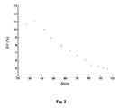
- the figure 2 illustrates an example of the evolution of the estimated prediction error ( Err ) by a response surface (approximate model), as a function of the number of simulations ( Nsim ) used to construct the response surface.
- the response surface approximates the output of the flow simulator corresponding to the oil flow of the tank after 10 years of production.
- This criterion allows a user to decide whether to add simulations to improve the predictive reliability of the model.
- the number p of simulations carried out at each iteration can be controlled by the user, depending on the number of machines available to perform simulations for example.
- step e) The addition of simulations in step e) is repeated, automatically, to satisfy a stopping criterion which is related to the degree of prediction desired by the user, defined in step a), by example average prediction of 5% of the response studied.
- a stopping criterion which is related to the degree of prediction desired by the user, defined in step a)
- An example of estimation of the prediction is obtained from the average of the cross-validation errors in each zone.
- the principle of optimization of the production scheme consists of defining different production scenarios, and for each of them, predicting production. This technique also makes it possible, in the same way, to economically evaluate a petroleum deposit.
- the approximate model is used because it is simple and analytical and, therefore, every estimate obtained by this model is immediate. This saves a lot of time.
- the use of this model allows the reservoir engineer to test as many scenarios as he wants, without worrying about the time required to perform a numerical flow simulation, and above all it allows him to take into account the uncertainties by testing different values of input parameters.
- the approximate analytical model is used with Monte Carlo or Quasi Monte Carlo direct sampling techniques (MCMC, Hypercube Latin, 3) in order to propagate the uncertainties of the input parameters on the selected simulator response (s).
- MCMC Monte Carlo or Quasi Monte Carlo direct sampling techniques
- the approximate model is used to perform an overall sensitivity analysis, so as to select the parameters influencing the production of the deposit, in order to carry out the measurements necessary for a better evaluation of the deposit.
- f 0 ⁇ ⁇ p ⁇ f x ⁇ dx and if ( he , ..., is ) ⁇ ( j1 , ..., jl ), then f ⁇ p ⁇ f i ⁇ 1 , ... , isf j ⁇ 1 , ... , jl ⁇ dx
- S i is called the first order sensitivity index for the factor x i . This index measures the part of the variance of the response explained by the effect of x i .
- S i, j for i ⁇ j, is called the second order sensitivity index. This index measures the proportion of response variance due to interactions between the effects of x i and x j .
- the total sensitivity index, S Ti for a particular parameter x i can also be very useful for measure the part of the variance of the response explained by all the effects in which x i plays a role.
- the global sensitivity analysis makes it possible to explain the variability of the responses as a function of the input parameters, through the definition of total or partial sensitivity indices. These indices can be estimated by Monte Carlo or Quasi Monte Carlo techniques to approximate the different multidimensional integrals, requiring a large sampling.
- the overall sensitivity analysis can not be used directly using a flow simulator.
- the sensitivity index calculations are performed using analytical models for each response. These analytical models are constructed as previously described.
- the Global Sensitivity Analysis (ASG) used in the invention does not have the usual limitations related to the hypotheses that other methods can be used that allow the calculation of standard sensitivity indices Spearman, Pearson, SRC, rank index, ...
- the only hypothesis is that the uncertain parameters are independent, which greatly expands the use of ASG using Sobol decomposition. This assumption is generally respected in reservoir engineering problems, since the links between parameters are known a priori.
- the Global Sensitivity Analysis (ASG) of the uncertain parameters on the simulator responses also makes it possible to evaluate the average effect of a parameter on a given response.
- This average effect can be used for example for controllable parameters, eg position a well, injection flow etc ... and is therefore a simple tool of behavior parameters.
- the use of the approximate model to make the ASG allows to determine the influential parameters, and how they are influential. It is thus possible to know the total impact of a parameter, as well as its combined impact with one or more other parameters on the production or economic response of the deposit.
- the ASG clearly allows a better understanding of the deposit's behavior.
- the determination of the average effects of the parameters is also a tool to characterize the average influence of a parameter, given the uncertainty of the other parameters on the responses in production or economic reservoir.
- the input parameters comprise stochastic fields, eg permeability, porosity, facies, etc.
- stochastic fields eg permeability, porosity, facies, etc.
- the uncertainty coming from the geostatistical maps is often neglected in the methods of uncertainty analysis based on plans. experience.
- the stochastic field is decomposed into a number n of components via the Karhunen-Loeve decomposition (M. Loève Probability Theory, Princeton University Press, 1955).
- the geostatistical techniques used in reservoir engineering to model the permeability and porosity quantities of rocks are mostly based on random Gaussian functions, discretized on a mesh covering the physical space of the reservoir.
- the Karhunen-Loève decomposition of a geostatistical model consists of representing it in the base formed of the eigenvectors of its covariance operator. This gives a functional representation of the random field.
- the method according to the invention is a tool for the analysis of the uncertainties of a flow simulator, and to help an engineer to reduce this uncertainty, focusing on the characterization of the parameters whose uncertainty contributes mainly to the poor characterization of the outputs.
- This method provides a robust and cost-effective tool (in terms of the number of simulations) for the global sensitivity analysis and the propagation of uncertainties. It allows the engineer to control the degree of approximation of his results by analyzing in real time the advantages in terms of prediction compared to the number of simulations carried out.
- the method allows the uncertainties of the geostatistical model (permeability, porosity, facies, etc.) to be taken into account by using surface response techniques and global sensitivity analysis.
Landscapes
- Life Sciences & Earth Sciences (AREA)
- Engineering & Computer Science (AREA)
- Geology (AREA)
- Mining & Mineral Resources (AREA)
- Physics & Mathematics (AREA)
- Environmental & Geological Engineering (AREA)
- Fluid Mechanics (AREA)
- General Life Sciences & Earth Sciences (AREA)
- Geochemistry & Mineralogy (AREA)
- Management, Administration, Business Operations System, And Electronic Commerce (AREA)
Abstract
Description
La présente invention concerne le domaine de l'exploration et l'exploitation de gisements pétroliers. Plus particulièrement l'invention concerne l'évaluation de tels gisements, par l'étude et l'optimisation de schémas de production de tels gisements pétroliers.The present invention relates to the field of exploration and exploitation of oil deposits. More particularly, the invention relates to the evaluation of such deposits, by studying and optimizing production patterns of such oil deposits.
Un schéma de production constitue une option de développement d'un gisement. Il regroupe tous les paramètres nécessaires à la mise en production d'un gisement. Ces paramètres peuvent être la position d'un puits, le niveau de complétion, la technique de forage...A production scheme is an option for developing a deposit. It groups all the parameters necessary for the production of a deposit. These parameters can be the position of a well, the level of completion, the drilling technique ...
L'étude d'un gisement comporte deux phases principales : une phase de caractérisation du réservoir et une phase de prévision de production.The study of a deposit has two main phases: a reservoir characterization phase and a production forecasting phase.
La phase de caractérisation du réservoir consiste à construire un modèle de réservoir. Un modèle de réservoir est une maquette décrivant la structure spatiale du gisement, sous forme d'une discrétisation de l'espace. Cette discrétisation se matérialise par un ensemble de mailles. A chacune de ces mailles, on associe des valeurs de propriétés caractérisant le gisement : porosité, perméabilité, lithologie, pression, nature des fluides,... Les ingénieurs n'ont accès qu'à une infime partie du gisement qu'ils étudient (mesures sur carottes, diagraphies, essais de puits, ...). Ils doivent extrapoler ces données ponctuelles sur la totalité du champ pétrolier pour construire un modèle de réservoir fiable. En conséquence, la notion d'incertitude doit être constamment prise en compte.The characterization phase of the reservoir consists of constructing a reservoir model. A reservoir model is a model describing the spatial structure of the deposit, in the form of a discretization of space. This discretization is materialized by a set of meshes. At each of these meshes, we associate values of properties characterizing the deposit: porosity, permeability, lithology, pressure, nature of the fluids, ... The engineers have access only to a small part of the deposit they study ( measurements on cores, logs, well tests, ...). They need to extrapolate these point data across the entire oil field to build a reliable reservoir model. Consequently, the notion of uncertainty must be constantly taken into account.
Pour la phase de prévision de production à un instant donné, pour améliorer cette production, ou, en général, pour augmenter le rendement économique du champ, le spécialiste possède un outil, appelé « simulateur d'écoulement ». Un simulateur d'écoulement est un logiciel permettant, entre autre, de modéliser la production d'un gisement en fonction du temps, à partir de mesures décrivant le gisement, c'est-à-dire, à partir du modèle de réservoir.For the production forecast phase at a given moment, to improve this production, or, in general, to increase the economic yield of the field, the specialist has a tool, called "flow simulator". A flow simulator is a software allowing, among other things, to model the production of a deposit as a function of time, from measurements describing the deposit, that is to say, from the reservoir model.
Un simulateur d'écoulement fonctionne en acceptant des paramètres en entrée, et en résolvant des équations physiques de mécanique des fluides en milieu poreux, pour délivrer des informations appelées réponses. L'ensemble des paramètres d'entrées est contenu dans le modèle de réservoir. Les propriétés associées aux mailles de ce modèles sont alors appelées paramètres. Ces paramètres sont notamment associés à la géologie du gisement, aux propriétés pétro-physiques, au développement du gisement et aux options numériques du simulateur. Les réponses (sorties) fournies par le simulateur sont, par exemple, la production d'huile, d'eau ou de gaz du réservoir et de chaque puit pour différents temps. Généralement, pour chacune des valeurs des différents paramètres d'entrée, le simulateur d'écoulement renvoie une seule valeur pour chaque réponse (sortie). Le simulateur d'écoulement est alors qualifié de déterministe.A flow simulator works by accepting input parameters, and solving physical fluid mechanics equations in porous media, to deliver information called responses. The set of input parameters is contained in the reservoir model. The properties associated with the meshes of this model are then called settings. These parameters are associated with the geology of the deposit, the petro-physical properties, the development of the deposit and the numerical options of the simulator. The responses (outputs) provided by the simulator are, for example, the production of oil, water or gas tank and each well for different times. Generally, for each of the values of the different input parameters, the flow simulator returns a single value for each response (output). The flow simulator is then qualified as deterministic.
Cependant, la majorité des paramètres d'entrée sont incertains. Ces incertitudes se traduisent par le fait que l'on ne peut pas attribuer une valeur unique, dont est sûr de la valeur, à un paramètre du modèle de réservoir. Par exemple, on ne peut pas assurer que la porosité en un point du gisement est de 20%. On peut au mieux considérer que la porosité est comprise entre 15% et 25% en ce point. Ceci est notamment dû au fait que les paramètres d'entrée sont déterminés à l'aide d'un nombre de mesures et informations limitées. Les réponses possibles du simulateur d'écoulement sont donc multiples, compte tenu de l'incertitude inhérente au modèle de réservoir. Dans notre exemple, il y aura une réponse du simulateur si la porosité est 15%, une réponse différente si la porosité est 20,5%... Il est ainsi indispensable de pouvoir quantifier l'incertitude sur les sorties du simulateur. De même, une correcte caractérisation de l'incertitude des paramètres d'entrée est indispensable. Il est également important de déterminer les paramètres d'entrée qui ont un effet significatif sur les réponses d'intérêts.However, the majority of input parameters are uncertain. These uncertainties result in the fact that one can not assign a single value, which is sure of value, to a parameter of the reservoir model. For example, we can not ensure that the porosity at one point of the deposit is 20%. It can best be considered that the porosity is between 15% and 25% at this point. This is because the input parameters are determined using a limited number of measurements and information. The possible responses of the flow simulator are therefore multiple, given the inherent uncertainty of the reservoir model. In our example, there will be a response from the simulator if the porosity is 15%, a different response if the porosity is 20.5% ... It is thus essential to be able to quantify the uncertainty on the outputs of the simulator. Similarly, a correct characterization of the uncertainty of the input parameters is essential. It is also important to determine input parameters that have a significant effect on interest responses.
Le spécialiste de l'exploitation d'un gisement pétrolier doit donc intégrer ces notions d'incertitudes dans l'évaluation d'un gisement, de façon à déterminer, par exemple, des conditions optimales de production.The specialist in the exploitation of an oil field must therefore integrate these notions of uncertainty into the evaluation of a deposit, so as to determine, for example, optimal production conditions.
Afin de bien caractériser l'impact de chaque incertitude sur la production de pétrole, de nombreux scénarios de production doivent être testés, et par conséquent, un nombre important de simulations de réservoir est nécessaire.In order to properly characterize the impact of each uncertainty on oil production, many production scenarios need to be tested, and as a result, a significant number of reservoir simulations are needed.
Cependant, dans l'industrie pétrolière, pour être de plus en plus fiables et prédictifs, la tendance est d'utiliser des simulateurs d'écoulements de plus en plus complexes, qui demandent un modèle de réservoir de plus en plus détaillé (plusieurs millions de mailles). Mais compte tenu du délai important requis pour effectuer une simulation d'écoulement, il ne peut pas être envisagé de tester tous les scénarios possibles via un simulateur d'écoulement.However, in the oil industry, to be more reliable and predictive, the trend is to use increasingly complex flow simulators, which require a more and more detailed reservoir model (several million mesh). But given the significant time required to perform a flow simulation, it can not be considered to test all possible scenarios via a flow simulator.
Pour éviter de réaliser un grand nombre de simulations, on connaît une technique, décrite dans le brevet
Cependant, toute surface de réponse commet une erreur de prédiction plus ou moins importante, selon la réponse qu'elle essaie d'approximer. En général, l'ajout d'information (i.e. de simulations) permet la construction d'une surface de réponse de plus en plus prédictive.However, any response surface makes a more or less important prediction error, depending on the response it tries to approximate. In general, the addition of information (i.e. simulations) allows the construction of an increasingly predictive response surface.
L'objet de l'invention est une méthode alternative, pour évaluer des schémas de production de gisements souterrain, en estimant la production de tels gisements à l'aide d'un modèle approché, et ajusté de façon itérative pour qu'il reproduise au mieux les réponses du simulateur, tout en maîtrisant le nombre de simulations nécessaires à sa construction.The object of the invention is an alternative method for evaluating underground deposit production patterns by estimating the production of such deposits using an approximate model, and iteratively adjusted to reproduce at better simulator responses, while controlling the number of simulations required for its construction.
L'invention concerne une méthode pour évaluer un schéma de production d'un gisement souterrain. Selon la méthode, on sélectionne des propriétés physiques caractérisant ledit gisement et ledit schéma de production. Ces propriétés constituent des paramètres d'entrée d'un simulateur d'écoulement permettant de simuler des réponses du gisement, telles que la production. On construit un modèle analytique approché permettant de prédire lesdites réponses du gisement. La méthode comporte également les étapes suivantes :
- on ajuste ledit modèle analytique approché à l'aide d'un processus itératif comportant les étapes suivantes :
- a)- on définit, pour chacune desdites réponses, un degré de précision Dp que l'on souhaite obtenir, ledit degré de précision Dp mesurant l'écart entre les réponses prédites par le modèle et celles simulées par le simulateur ;
- b)- on calcule un degré de précision Dp(M) des prédictions du modèle analytique approché ;
- c)- si cette valeur Dp(M) est inférieure au degré de prédiction souhaité Dp , le processus itératif s'arrête, sinon on poursuit par les étapes suivantes :
- d)- on construit un plan d'expériences de façon à sélectionner des simulations à réaliser, pertinentes pour ajuster ledit modèle ;
- e)- on réalise les simulations sélectionnées par le plan d'expérience à l'aide du simulateur d'écoulement, puis, pour chacune des réponses simulées par le simulateur, on ajuste ledit modèle analytique à l'aide d'une méthode d'approximation, de façon à ajuster les réponses prédites par le modèle à celles simulées par le simulateur ;
- f)- on recommence à l'étape b), jusqu'à ce que le degré de précision souhaité Dp soit atteint ; et
- on évalue ledit schéma de production, en analysant lesdites réponses dudit gisement prédites par ledit modèle analytique approché.
- said approximate analytical model is adjusted using an iterative process comprising the following steps:
- a) - one defines, for each of said responses, a degree of precision D p that one wishes to obtain, said degree of precision D p measuring the difference between the responses predicted by the model and those simulated by the simulator;
- b) - a degree of precision D p (M) of the predictions of the approximate analytical model is calculated;
- c) - if this value D p (M) is less than the desired degree of prediction D p , the iterative process stops, otherwise the following steps are continued:
- d) - one builds a plan of experiments so as to select simulations to realize, relevant to adjust said model;
- e) - the simulations selected by the experimental plane are carried out using the flow simulator, then, for each of the simulated responses simulated by the simulator, said analytical model is adjusted using a method of approximation, so as to adjust the responses predicted by the model to those simulated by the simulator;
- f) - is repeated in step b) until the desired degree of accuracy D p is reached; and
- said production scheme is evaluated by analyzing said responses of said deposit predicted by said approximate analytical model.
Selon l'invention, on peut modifier le degré de précision souhaité Dp à chacune des itérations. Les paramètres d'entrée peuvent être incertains, c'est-à-dire que les valeurs de ces paramètres d'entrée sont incertaines.According to the invention, it is possible to modify the desired degree of precision D p at each of the iterations. The input parameters may be uncertain, that is, the values of these input parameters are uncertain.
Les réponses du gisement, prédites par le modèle analytique approché, peuvent être analysées en quantifiant une influence de chacun des paramètres d'entrée sur chacune des réponses, à l'aide d'une analyse de sensibilité globale, dans laquelle on calcule des indices de sensibilité en utilisant le modèle analytique. A l'aide de cette analyse de sensibilité globale, on peut les paramètres les plus influents sur les réponses du gisement, et définir ainsi des mesures à réaliser pour faire décroître une incertitude sur les réponses du gisement.The deposit responses, predicted by the approximate analytical model, can be analyzed by quantifying an influence of each of the input parameters on each of the responses, using an overall sensitivity analysis, in which sensitivity using the analytical model. With the help of this global sensitivity analysis, we can use the most influential parameters on the deposit's responses, and thus define the measures to be taken to reduce uncertainty in the deposit's responses.
Selon l'invention, si les paramètres d'entrée comportent au moins un champ stochastique, on peut décomposer ce champ stochastique en un nombre n de composantes via une décomposition de Karhunen-Loeve. On sélectionne alors les composantes du champ stochastique ayant un impact sur les réponses à l'aide de l'analyse de sensibilité globale.According to the invention, if the input parameters comprise at least one stochastic field, it is possible to decompose this stochastic field into a number n of components via a Karhunen-Loeve decomposition. The components of the stochastic field that have an impact on the responses are then selected using the global sensitivity analysis.
D'autres caractéristiques et avantages de la méthode selon l'invention, apparaîtront à la lecture de la description ci-après d'exemples non limitatifs de réalisations, en se référant aux figures annexées et décrites ci-après.Other characteristics and advantages of the method according to the invention will appear on reading the following description of nonlimiting examples of embodiments, with reference to the appended figures and described below.
-
la
figure 1 représente un canevas de la méthode de gestion des incertitudes selon l'invention.thefigure 1 represents a framework of the uncertainty management method according to the invention. -
la
figure 2 montre un exemple d'évolution de l'erreur de prédiction estimée (en %) par une surface de réponse (modèle approché).thefigure 2 shows an example of evolution of the estimated prediction error (in%) by a response surface (approximate model).
La méthode selon l'invention permet d'optimiser le schéma de production d'un gisement pétrolier. La méthode est schématisée par le diagramme de la
- 1- Sélection et caractérisation des incertitudes des paramètres d'entrée du simulateur
- 2- Construction d'un modèle analytique approché du simulateur
- 3- Ajustement du modèle analytique approché
- 4- Optimisation du schéma de production du gisement.
- 1- Selection and characterization of the uncertainties of the input parameters of the simulator
- 2- Construction of an approximate analytical model of the simulator
- 3- Adjustment of the approximate analytical model
- 4- Optimization of the deposit production scheme.
Tout simulateur d'écoulement permet notamment de calculer la production d'hydrocarbures ou d'eau en fonction du temps, à partir de paramètres physiques caractéristiques du gisement pétrolier, tels que le nombre de couches du réservoir, la perméabilité des couches, la force de l'aquifère, la position des puits de pétrole, etc.Any flow simulator makes it possible to calculate the production of hydrocarbons or water as a function of time, based on physical parameters characteristic of the oil reservoir, such as the number of layers of the reservoir, the permeability of the layers, the force of the the aquifer, the position of the oil wells, etc.
Ces paramètres physiques constituent les entrées du simulateur d'écoulement. Elles sont obtenues par des mesures effectuées en laboratoire sur des carottes et des fluides prélevés sur le gisement pétrolier, par diagraphies (mesures réalisées le long d'un puits), par essais de puits, etc.These physical parameters constitute the inputs of the flow simulator. They are obtained by laboratory measurements on cores and fluids taken from the oil field, by logging (measurements along a well), by well tests, etc.
Parmi les paramètres physiques caractéristiques du gisement pétrolier, on sélectionne de préférence des paramètres d'entrée ayant une influence sur les profils de production d'hydrocarbures ou d'eau par le gisement. La sélection des paramètres peut se faire soit par rapport à la connaissance physique du gisement pétrolier, soit par une étude de sensibilité. Par exemple, on peut mettre en oeuvre un test statistique de Student ou de Fischer.Among the physical parameters characteristic of the oil field, it is preferable to select input parameters having an influence on the profiles of production of hydrocarbons or water by the deposit. The selection of the parameters can be done either with respect to the physical knowledge of the oil field, or by a sensitivity study. For example, it is possible to implement a Student or Fischer statistical test.
Des paramètres peuvent être intrinsèques au réservoir pétrolier. Par exemple, on peut considérer les paramètres suivants : perméabilité de certaines couches du réservoir, force de l'aquifère, saturation d'huile résiduelle après balayage à l'eau...Parameters may be intrinsic to the oil reservoir. For example, the following parameters may be considered: permeability of certain layers of the reservoir, aquifer strength, residual oil saturation after sweeping with water ...
Des paramètres peuvent correspondre à des options de développement du gisement. Ces paramètres peuvent être la position d'un puits, le niveau de complétion, la technique de forage.Parameters may correspond to deposit development options. These parameters can be the position of a well, the level of completion, the drilling technique.
Après sélection de ces paramètres d'entrée, on caractérise les incertitudes associées à ces paramètres. On peut par exemple remplacer une valeur d'un paramètre par un intervalle de variation de ce paramètre.After selecting these input parameters, the uncertainties associated with these parameters are characterized. For example, a value of a parameter can be replaced by a variation interval of this parameter.
Le simulateur d'écoulement étant un outil complexe et gourmand en temps de calcul, on ne peut pas l'utiliser pour tester tous les scénarios en tenant compte de toutes les incertitudes des paramètres. On construit alors un modèle analytique approché du comportement du gisement pétrolier. Ce modèle approché est également appelé « surface de réponse ». Il consiste en un ensemble de formules analytiques, chacune traduisant le comportement d'une réponse donnée du simulateur d'écoulement. Ces formules analytiques sont fonction d'un nombre réduit de paramètres, et elles sont construites à partir d'un nombre limité de simulations.Since the flow simulator is a complex and time-consuming tool, it can not be used to test all scenarios taking into account all the uncertainties of the parameters. An approximate analytical model of the behavior of the oil field is then constructed. This approximate model is also called "response surface". It consists of a set of analytical formulas, each of which translates the behavior of a given response of the flow simulator. These analytic formulas are based on a small number of parameters, and they are constructed from a limited number of simulations.
Ce modèle approché traduit le comportement de réponses données, par exemple le cumulé d'huile produit à 10 ans, en fonction de quelques paramètres d'entrée. Ainsi, pour chaque réponse (sortie) du simulateur d'écoulement, nécessaire à l'optimisation de la production ou l'évaluation du gisement, on associe une formule analytique permettant d'approximer cette réponse à partir de paramètres d'entrée.This approximate model reflects the behavior of given responses, for example the cumulative oil produced at 10 years, according to some input parameters. Thus, for each response (output) of the flow simulator, necessary for the optimization of production or the evaluation of the deposit, we associate an analytical formula for approximating this response from input parameters.
Pour construire ce modèle approché du simulateur d'écoulement, on combine deux techniques : une méthode d'approximation et une méthode de plans d'expériences.To construct this approximate model of the flow simulator, two techniques are combined: an approximation method and a sample plan method.
Les plans d'expériences permettent de déterminer le nombre et la localisation, dans l'espace des paramètres d'entrée, d'un nombre réduit de simulations à réaliser pour avoir le maximum d'informations pertinentes, au coût le plus faible possible.Experimental designs allow to determine the number and location, in the space of the input parameters, of a reduced number of simulations to realize to have the maximum of relevant information, at the lowest possible cost.
La technique des plans d'expériences est décrite par exemple dans
Un plan indique différents jeux de valeurs pour les paramètres incertains. Chaque jeu de valeurs des paramètres incertains est utilisé pour effectuer une simulation d'écoulement. Dans l'espace des paramètres d'entrée, chaque simulation représente un point. Chaque point correspond à des valeurs pour les paramètres incertains et donc à un modèle de réservoir possible. Le choix de ces points, grâce aux plans d'expériences, peut faire intervenir de nombreux types de critères, comme l'orthogonalité ou le remplissage de l'espace (« space-filling »).A plan indicates different sets of values for the uncertain parameters. Each set of uncertain parameter values is used to perform a flow simulation. In the input parameter space, each simulation represents a point. Each point corresponds to values for the uncertain parameters and therefore to a possible reservoir model. The choice of these points, thanks to the experimental designs, can involve many types of criteria, such as orthogonality or space-filling.
Pour cette étape "exploratoire", le choix des points de simulation peut être réalisé grâce à différents types de plans d'expériences, par exemple, les plans factoriels, les plans composites, les plans de distance maximum, etc. On peut également utiliser un plan d'expérience de type Hypercube Latin Maximin ou Sobol LP-τ (
Après la construction de ce plan d'expériences, et lorsque les simulations d'écoulement sont réalisées, une méthode d'approximation est utilisée pour déterminer un modèle approché. Ce modèle approche les réponses du simulateur d'écoulement. De façon très simplifiée, on peut imaginer qu'en réalisant quatre simulations, on obtient quatre couples (paramètre d'entrée, réponse). On estime alors une relation respectant au mieux ces couples.After the construction of this experimental design, and when the flow simulations are performed, an approximation method is used to determine an approximate model. This model approaches the responses of the flow simulator. In a very simplified way, we can imagine that by performing four simulations, we obtain four couples (input parameter, response). We then estimate a relationship that best respects these couples.
En pratique, les paramètres et les sorties étant multiples, on peut utiliser, comme méthode d'approximation, des polynômes du premier ou du deuxième ordre, des réseaux de neurones, des machines à support vectoriel ou éventuellement des polynômes d'ordre supérieur à deux. De nombreuses autres techniques sont connues des spécialistes, telles que les méthodes à base d'ondelettes, de SVM, de noyau hilbertien auto reproduisant, ou encore la régression non-paramétrique basée sur un processus Gaussien ou krigeage (
Ainsi, pour construire le modèle approché, on procède de la façon suivante :
- on construit un plan d'expériences de façon à sélectionner un nombre restreint de simulations ;
- on réalise les simulations sélectionnées par le plan d'expérience à l'aide du simulateur d'écoulement, à partir de paramètres d'entrée sélectionnés ;
- pour chacune des réponses du simulateur, on définit une formule analytique reliant les paramètres d'entrée sélectionnés à la réponse (issue des simulations), à l'aide d'une méthode d'approximation.
- an experimental design is constructed to select a limited number of simulations;
- the simulations selected by the experimental plane are carried out using the flow simulator from selected input parameters;
- for each of the responses of the simulator, we define an analytical formula connecting the selected input parameters to the response (resulting from the simulations), using an approximation method.
Le modèle approché, ainsi déterminé, permet de prédire les sorties du simulateur d'écoulement avec une certaine précision. Selon l'invention, la méthode comporte une mesure de la précision de prédiction de ce modèle de façon à définir un critère d'évaluation associé à la précision du modèle approché construit. La
Ce critère permet à un utilisateur de décider de l'ajout éventuel de simulations afin d'améliorer la fiabilité de prédiction du modèle.This criterion allows a user to decide whether to add simulations to improve the predictive reliability of the model.
Le degré de prédiction requis est obtenu de façon itérative. Cette étape se décompose de la façon suivante :
- a)- on définit un degré de précision Dp de la prédiction du modèle approché que l'on souhaite obtenir pour chaque réponse du simulateur que l'on veut analyser.
- b)- on estime le degré de prédiction Dp(M) du modèle analytique approché. Cette estimation peut se faire en utilisant des méthodes de type validation croisée ou bootstrap.
- c)- Si cette valeur Dp(M) est inférieure au degré de prédiction souhaité Dp , le processus itératif automatique s'arrête, sinon on poursuit par les étapes suivantes :
- d)- on sélectionne p nouvelles combinaisons de paramètres d'entrée dans l'espace des paramètres d'entrée, au moyen d'une méthode adaptative. Une méthode adaptative consiste à ajouter de l'information aux endroits où il en manque, et où le modèle approché n'est pas suffisamment prédictif. De telles méthodes sont bien connues des spécialistes.
- e)- on réalise les p simulations correspondantes, et l'on modifie le modèle approché en conséquences.
- f)- puis l'on recommence à l'étape b), jusqu'à ce que le degré de précision soit atteint. On peut également recommencer à l'étape a), de façon à définir un nouveau degrés de précision.
- a) - one defines a degree of precision D p of the prediction of the approximate model that one wishes to obtain for each answer of the simulator that one wants to analyze.
- b) - we estimate the degree of prediction D p (M) of the approximate analytical model. This estimate can be done using cross validation or bootstrap methods.
- c) - If this value D p (M) is lower than the desired degree of prediction D p , the automatic iterative process stops, otherwise we continue with the following steps:
- d) - selecting p new combinations of input parameters in the space of input parameters by means of an adaptive method. An adaptive method is to add information where it is missing, and where the approximate model is not predictive enough. Such methods are well known to those skilled in the art.
- e) - p corresponding simulations are carried out, and it changes the approximate model accordingly.
- f) - then one starts again in step b), until the degree of precision is reached. We can also start again at step a), so as to define a new degree of precision.
Le nombre p de simulations réalisées à chaque itération peut être contrôlé par l'utilisateur, en fonction du nombre de machines disponibles pour réaliser des simulations par exemple.The number p of simulations carried out at each iteration can be controlled by the user, depending on the number of machines available to perform simulations for example.
Le modèle approché ainsi obtenu permet de prédire les réponses quasi instantanément (en temps de calcul), et permet donc de remplacer le simulateur d'écoulement coûteux en temps de calcul. On peut donc tester un grand nombre de scénarios de production, tout en tenant compte de l'incertitude de chaque paramètre d'entrée.The approximate model thus obtained makes it possible to predict the responses almost instantaneously (in computing time), and thus makes it possible to replace the expensive flow simulator in computing time. We can therefore test a large number of production scenarios, while taking into account the uncertainty of each input parameter.
Les méthodes utilisées pour sélectionner de nouveaux points dans l'espace des paramètres à l'étape d) peuvent être diverses. On peut par exemple se baser sur une méthode décrite dans les documents suivants :
-
Scheidt C., Zabalza-Mezghani I., Feraille M., Collombier D.: "Adaptive Evolutive Experimental Designs for Uncertainty Assessment - An innovative exploitation of geostatistical techniques", IAMG, Toronto, 21-26 August, Canada, 2005 -
Busby D., Farmer C.L., Iske A.: "Hierarchical Nonlinear Approximation for Experimental Design and Statistical Data Fitting". SIAM J. Sci. Comput. 29, 1, 49-69, 2007
-
Scheidt C., Zabalza-Mezghani I., Feraille M., Collombier D .: "Adaptive Evolutive Experimental Designs for Uncertainty Assessment - An Innovative Exploitation of Geostatistical Techniques", IAMG, Toronto, 21-26 August, Canada, 2005 -
Busby D., Farmer CL, Iske A .: "Hierarchical Nonlinear Approximation for Experimental Design and Statistical Data Fitting". SIAM J. Sci. Comput. 29, 1, 49-69, 2007
L'ajout de simulations à l'étape e) est répété, automatiquement, jusqu'à satisfaire un critère d'arrêt qui est lié au degré de prédiction souhaité par l'utilisateur, défini à l'étape a), par exemple prédiction moyenne de 5% de la réponse étudiée. Un exemple d'estimation de la prédiction est obtenu à partir de la moyenne des erreurs de validation croisée dans chaque zone.The addition of simulations in step e) is repeated, automatically, to satisfy a stopping criterion which is related to the degree of prediction desired by the user, defined in step a), by example average prediction of 5% of the response studied. An example of estimation of the prediction is obtained from the average of the cross-validation errors in each zone.
Les réponses d'intérêts choisies peuvent correspondre à des sorties directes du simulateur d'écoulement ou à des combinaisons et interpolations de sorties. Par exemple ont peut s'intéresser:
- uniquement à la production cumulée de l'huile (gaz, eau) du réservoir au temps final de production,
- à la production cumulée de l'huile (gaz, eau) du réservoir pour différents temps,
- à l'ajout de la production d'huile et de la production d'eau,
- à la production d'huile pour des valeurs fixées de water cut (ou de production d'eau),
- à la durée du plateau du profil de production,...
- only to the cumulative production of the oil (gas, water) of the tank at the final time of production,
- the cumulative production of the oil (gas, water) of the tank for different times,
- the addition of oil production and water production,
- the production of oil for fixed values of water cut (or water production),
- to the shelf life of the production profile, ...
De plus on peut facilement rajouter des incertitudes économiques et les combiner aux incertitudes techniques pour définir des réponses associées à la valeur économique du gisement comme par exemple la Valeur Actuelle Nette (VAN) et ne pas se limiter à des réponses techniques (de production d'huile, de gaz, d'eau, ...). Une telle méthode est décrite dans la demande
Le principe d'optimisation du schéma de production consiste à définir différents scénarios de production, et pour chacun d'eux, prédire la production. Cette technique permet également, de la même façon, d'évaluer économiquement un gisement pétrolier.The principle of optimization of the production scheme consists of defining different production scenarios, and for each of them, predicting production. This technique also makes it possible, in the same way, to economically evaluate a petroleum deposit.
Au cours de cette phase de prévision de production, le modèle approché est utilisé parce qu'il est simple et analytique et, donc, chaque estimation obtenue par ce modèle est immédiate. Cela constitue une économie de temps considérable. L'utilisation de ce modèle autorise l'ingénieur réservoir à tester autant de scénarios qu'il le souhaite, sans se soucier des délais nécessaires pour effectuer une simulation numérique d'écoulement, et surtout cela lui permet de prendre en compte les incertitudes en testant différentes valeurs de paramètres d'entrée.During this production forecasting phase, the approximate model is used because it is simple and analytical and, therefore, every estimate obtained by this model is immediate. This saves a lot of time. The use of this model allows the reservoir engineer to test as many scenarios as he wants, without worrying about the time required to perform a numerical flow simulation, and above all it allows him to take into account the uncertainties by testing different values of input parameters.
Le modèle analytique approché est utilisé avec des techniques d'échantillonnage direct de type Monte Carlo ou Quasi Monte Carlo (MCMC, Hypercube Latin, ...) pour pouvoir propager les incertitudes des paramètres d'entrée sur la ou les réponses du simulateur choisies.The approximate analytical model is used with Monte Carlo or Quasi Monte Carlo direct sampling techniques (MCMC, Hypercube Latin, ...) in order to propagate the uncertainties of the input parameters on the selected simulator response (s).
On obtient ainsi les distributions de probabilité associées aux sorties du simulateur. Ces distributions sont utiles pour pouvoir prendre des décisions sur l'exploitation du gisement en question, compte tenu de la production ou valeur économique possible et de l'incertitude associée.This gives the probability distributions associated with the outputs of the simulator. These distributions are useful for making decisions about the exploitation of the deposit in question, taking into account the potential production or economic value and the associated uncertainty.
Selon un mode de réalisation particulier, on utilise le modèle approché pour réaliser une analyse de sensibilité globale, de façon à sélectionner les paramètres influant la production du gisement, afin de réaliser les mesures nécessaires à une meilleure évaluation du gisement.According to a particular embodiment, the approximate model is used to perform an overall sensitivity analysis, so as to select the parameters influencing the production of the deposit, in order to carry out the measurements necessary for a better evaluation of the deposit.
Il est par exemple intéressant de savoir que l'activité de l'aquifère ou la perméabilité d'une couche géologique particulière joue un rôle prépondérant sur les résultats de production future du gisement.For example, it is interesting to know that the activity of the aquifer or the permeability of a particular geological layer plays a major role in the future production results of the deposit.
L'Analyse de Sensibilité Globale (ASG) des paramètres incertains sur les réponses du simulateur permet d'analyser de façon détaillée l'impact de l'incertitude de chaque paramètre ou groupe de paramètre incertain, sur l'incertitude des réponses du simulateur. Une telle technique est décrite dans :
-
Saltelli, K. Chan and M. Scott: "Sensitivity Analysis", New York, Wiley, 2000 -
Oakley and A. O'Hagan: "Probabilistic sensitivity analysis of complex models: A Bayesian approach", J. Roy. Statist. Soc. Ser. B, 16, pp. 751-769, 2004
-
Saltelli, K. Chan and M. Scott: "Sensitivity Analysis", New York, Wiley, 2000 -
Oakley and A. O'Hagan: "Probabilistic sensitivity analysis of complex models: A Bayesian approach", J. Roy. Statist. Soc. Ser. B, 16, pp. 751-769, 2004
Pour décrire la méthode, on considère un modèle mathématique décrit par une fonction f(x), x = (xl, ..., xp ), et défini dans espace à p dimensions Ω p = {x|0 ≤ xi ≤ 1;i = 1,...p}.To describe the method, we consider a mathematical model described by a function f (x), x = ( x l , ..., x p ), and defined in p-space p Ω p = {x | 0 ≤ x i ≤ 1; i = 1, ... p }.
L'idée principale de la décomposition de Sobol est de décomposer f(xl,...,xp) de la façon suivante : 

Selon cette définition, on peut écrire : ![]()
![]()
![]()
![]()
Sobol a montré que la décomposition de f(x1,...,xp) est unique et que tous les termes peuvent être évaluées via des intégrales multidimensionnelles : 

La variance totale V de ƒ(x) peut alors s'écrire : 
![]()
The total variance V of ƒ (x) can then be written: ![]()
Puis, pour expliquer la part de la variance des réponses due aux paramètres d'entrées, l'indice de sensibilité suivant peut être défini : 
Si est appelé l'indice de sensibilité de première ordre pour le facteur xi . Cet indice mesure la part de la variance de la réponse expliquée par l'effet de xi . S i is called the first order sensitivity index for the factor x i . This index measures the part of the variance of the response explained by the effect of x i .
Si,j, pour i ≠ j, est appelé l'indice de sensibilité de second ordre. Cet indice mesure la part de la variance de la réponse due aux interactions entre les effets de xi et xj . S i, j , for i ≠ j, is called the second order sensitivity index. This index measures the proportion of response variance due to interactions between the effects of x i and x j .
L'indice de sensibilité total, STi pour un paramètre particulier xi , défini comme la somme de tous les indices de sensibilité impliquant les paramètres, peut également être très utile pour mesurer la part de la variance de la réponse expliquée par tous les effets dans lesquels xi joue un rôle.The total sensitivity index, S Ti for a particular parameter x i , defined as the sum of all the sensitivity indices involving the parameters, can also be very useful for measure the part of the variance of the response explained by all the effects in which x i plays a role.
![]()
![]()
L'analyse de sensibilité globale permet d'expliquer la variabilité des réponses en fonction des paramètres d'entrée, à travers la définition d'indices de sensibilité total ou partiel. Ces indices peuvent être estimés par des techniques de Monte Carlo ou Quasi Monte Carlo pour approximer les différentes intégrales multidimensionnelles, nécessitant un large échantillonnage.The global sensitivity analysis makes it possible to explain the variability of the responses as a function of the input parameters, through the definition of total or partial sensitivity indices. These indices can be estimated by Monte Carlo or Quasi Monte Carlo techniques to approximate the different multidimensional integrals, requiring a large sampling.
Ainsi, l'analyse de sensibilité globale ne peut pas être utilisée directement en utilisant un simulateur d'écoulement. Selon l'invention, les calculs des indices de sensibilité sont effectués en utilisant des modèles analytiques pour chaque réponses, Ces modèles analytiques sont construits comme décrits précédemment.Thus, the overall sensitivity analysis can not be used directly using a flow simulator. According to the invention, the sensitivity index calculations are performed using analytical models for each response. These analytical models are constructed as previously described.
L'Analyse de Sensibilité Globale (ASG) utilisée dans l'invention n'a pas les limitations classiques liées aux hypothèses que peuvent avoir d'autres méthodes permettant les calculs d'indices de sensibilité type Spearman, Pearson, SRC, indice de rang, ... La seule hypothèse est le fait que les paramètres incertains sont indépendants, ce qui élargi grandement l'utilisation de l'ASG utilisant la décomposition de Sobol. Cette hypothèse est généralement respectée dans les problèmes d'ingénierie de réservoir, puisque les liens entre paramètres sont connus a priori.The Global Sensitivity Analysis (ASG) used in the invention does not have the usual limitations related to the hypotheses that other methods can be used that allow the calculation of standard sensitivity indices Spearman, Pearson, SRC, rank index, ... The only hypothesis is that the uncertain parameters are independent, which greatly expands the use of ASG using Sobol decomposition. This assumption is generally respected in reservoir engineering problems, since the links between parameters are known a priori.
Au cours de cette analyse, on détermine la contribution de l'incertitude de chaque paramètre à la variance totale de la (ou les) réponse(s). Le principe consiste à calculer plusieurs indices de sensibilité (premier, deuxième, ... Nième ordre et indices totaux) permettant de connaître l'influence précise de chaque paramètre ou groupe de paramètres sur les réponses d'intérêt. Ces indices sont calculés par des formules nécessitant le calcul d'intégrales multiples pouvant être réalisé de manière approximative par des techniques de Monte Carlo ou Quasi Monte Carlo.During this analysis, we determine the contribution of the uncertainty of each parameter to the total variance of the (or the) response (s). The principle consists in calculating several sensitivity indices (first, second, ... Nth order and total indices) allowing to know the precise influence of each parameter or group of parameters on the responses of interest. These indices are calculated by formulas requiring the calculation of multiple integrals that can be performed approximately by Monte Carlo or Quasi Monte Carlo techniques.
L'Analyse de Sensibilité Globale (ASG) des paramètres incertains sur les réponses du simulateur permet également d'évaluer l'effet moyen d'un paramètre sur une réponse donnée. Cet effet moyen peut être utilisé par exemple pour des paramètres contrôlables, e.g. position d'un puit, débit d'injection etc... et constitue donc un outil simple de comportement des paramètres.The Global Sensitivity Analysis (ASG) of the uncertain parameters on the simulator responses also makes it possible to evaluate the average effect of a parameter on a given response. This average effect can be used for example for controllable parameters, eg position a well, injection flow etc ... and is therefore a simple tool of behavior parameters.
L'utilisation du modèle approché afin de faire de l'ASG, permet de déterminer les paramètres influents, et la façon dont ils sont influents. Il est ainsi possible de connaître l'impact total d'un paramètre, ainsi que son impact combiné avec un ou plusieurs autres paramètres sur la réponse en production ou économique du gisement. L'ASG permet clairement une meilleure compréhension du comportement du gisement. De plus, la détermination des effets moyens des paramètres est aussi un outil permettant caractériser l'influence moyenne d'un paramètre, compte tenue de l'incertitude sur les autres paramètres sur les réponses en production ou économique du réservoir.The use of the approximate model to make the ASG, allows to determine the influential parameters, and how they are influential. It is thus possible to know the total impact of a parameter, as well as its combined impact with one or more other parameters on the production or economic response of the deposit. The ASG clearly allows a better understanding of the deposit's behavior. In addition, the determination of the average effects of the parameters is also a tool to characterize the average influence of a parameter, given the uncertainty of the other parameters on the responses in production or economic reservoir.
Enfin, on peut déterminer les mesures supplémentaires à réaliser pour mieux caractériser le gisement et ainsi faire décroître l'incertitude sur la production future. La quantification de l'influence des paramètres incertains sur la production du gisement permet de déterminer les paramètres les plus influents. Ainsi, pour limiter l'incertitude sur la production ou l'économie future du gisement, on caractérise d'abord les paramètres les plus influents. L'utilisation de la méthodologie décrite donne donc les moyens à l'ingénieur réservoir de déterminer les paramètres qui doivent être mieux définis, et donc, donne un guide dans le choix des nouvelles mesures à réaliser (logging, carottage, SCAL, ...). Une fois les paramètres influents mieux caractériser par mesures, il est alors possible d'utiliser à nouveau la méthodologie décrite afin de propager l'incertitude pour quantifier la nouvelle incertitude sur les réponses de production ou économique du réservoir.Finally, additional measures can be determined to better characterize the deposit and thus reduce uncertainty about future production. Quantifying the influence of uncertain parameters on the production of the deposit allows the most influential parameters to be determined. Thus, to limit uncertainty about the production or future economy of the deposit, the most influential parameters are first characterized. The use of the described methodology thus gives the means to the reservoir engineer to determine the parameters which must be better defined, and thus, gives a guide in the choice of the new measurements to realize (logging, coring, SCAL, ... ). Once influencing parameters better characterize by measurements, it is then possible to use again the described methodology in order to propagate the uncertainty to quantify the new uncertainty on the production or economic responses of the reservoir.
La propagation, l'analyse de sensibilité globale et le calcul des effets moyens requièrent plusieurs milliers d'évaluation de la ou des réponses associées. Cela rend donc ces méthodes inutilisables directement avec des gros codes numériques (comme c'est le cas pour les simulateurs d'écoulement), d'où l'intérêt de construire des modèles approché prédictifs, permettant d'utiliser ces techniques très intéressantes pour les réponses qu'elles apportent à des questions métiers.Propagation, global sensitivity analysis and average effects calculation require several thousand evaluations of the associated response (s). This makes these methods unusable directly with large numerical codes (as is the case for flow simulators), hence the interest of constructing predictive approximate models, allowing to use these very interesting techniques for their answers to business questions.
Selon un autre mode de réalisation, les paramètres d'entrées comporte des champs stochastiques, e.g. perméabilité, porosité, faciès,... L'incertitude provenant des cartes géostatistiques est souvent négligée dans les méthodes d'analyse d'incertitude basée sur des plans d'expérience.According to another embodiment, the input parameters comprise stochastic fields, eg permeability, porosity, facies, etc. The uncertainty coming from the geostatistical maps is often neglected in the methods of uncertainty analysis based on plans. experience.
Dans le cas de paramètres de type champ stochastique on décompose le champ stochastique en un nombre n de composantes via la décomposition de Karhunen-Loeve (M.M. Loève. Probability Theory. Princeton University Press, 1955.). Les techniques géostatistiques utilisés en ingénierie de réservoir pour modéliser les grandeurs de perméabilité et de porosité des roches, sont pour la plupart basées sur des fonctions aléatoires gaussiennes, discrétisés sur un maillage couvrant l'espace physique du réservoir. La décomposition de Karhunen-Loève d'un modèle géostatistique consiste à représenter celle-ci dans la base formée des vecteurs propres de son opérateur de covariance. On obtient ainsi une représentation fonctionnelle du champ aléatoire. En ne conservant qu'un nombre limité de composantes dans cette représentation, on obtient une approximation du champ aléatoire qui représente une part quantifiable de la variance du processus. En effet, à chaque terme de la décomposition est attribuée une part de la variance globale qui est égale à la valeur propre associée au vecteur propre correspondant. On peut ainsi quantifier l'erreur d'approximation en terme de variance. Le nombre de composantes nécessaires à reproduire le modèle géostatistique est souvent assez élevé. Des tests numériques ont montrés qu'une centaine de composantes peuvent être nécessaires dans certains cas. Pourtant, dans beaucoup de cas, seule la variation d'un nombre limité de ces composantes va impacter les réponses en production simulées du modèle de réservoir, par exemple le cumulé d'huile après 10 ans de production. Selon l'invention, on sélectionne les composantes du champ stochastique ayant un impact sur les réponses d'intérêts simulées, à l'aide d'une analyse de sensibilité globale avec un modèle approché comme indiqué dans les étapes précédentes.In the case of stochastic field type parameters, the stochastic field is decomposed into a number n of components via the Karhunen-Loeve decomposition (M. Loève Probability Theory, Princeton University Press, 1955). The geostatistical techniques used in reservoir engineering to model the permeability and porosity quantities of rocks are mostly based on random Gaussian functions, discretized on a mesh covering the physical space of the reservoir. The Karhunen-Loève decomposition of a geostatistical model consists of representing it in the base formed of the eigenvectors of its covariance operator. This gives a functional representation of the random field. By keeping only a limited number of components in this representation, we obtain an approximation of the random field which represents a quantifiable part of the variance of the process. Indeed, at each term of the decomposition is allocated a part of the global variance which is equal to the eigenvalue associated with the corresponding eigenvector. It is thus possible to quantify the approximation error in terms of variance. The number of components needed to reproduce the geostatistical model is often quite high. Numerical tests have shown that a hundred components may be needed in some cases. However, in many cases, only the variation of a limited number of these components will impact the simulated production responses of the reservoir model, for example cumulative oil after 10 years of production. According to the invention, the components of the stochastic field having an impact on the simulated interest responses are selected, using an overall sensitivity analysis with an approximate model as indicated in the previous steps.
La méthode selon l'invention constitue un outil pour l'analyse des incertitudes d'un simulateur d'écoulement, et pour aider un ingénieur à réduire cette incertitude, en se focalisant sur la caractérisation des paramètres dont l'incertitude contribue de façon principale à la mauvaise caractérisation des sorties.The method according to the invention is a tool for the analysis of the uncertainties of a flow simulator, and to help an engineer to reduce this uncertainty, focusing on the characterization of the parameters whose uncertainty contributes mainly to the poor characterization of the outputs.
Cette méthode fournit un outil robuste et à moindre coût (en termes du nombre de simulations) pour l'analyse de sensibilité globale et la propagation des incertitudes. Elle permet à l'ingénieur de contrôler le degré d'approximation de ses résultats en analysant en temps réel les avantages en termes de prédiction par rapport au nombre de simulations effectuées.This method provides a robust and cost-effective tool (in terms of the number of simulations) for the global sensitivity analysis and the propagation of uncertainties. It allows the engineer to control the degree of approximation of his results by analyzing in real time the advantages in terms of prediction compared to the number of simulations carried out.
L'analyse de sensibilité globale et l'effet moyen des paramètres permettent de voir l'impact de l'incertitude d'un paramètre sur l'incertitude globale d'une réponse, et donne donc un guide dans le choix des nouvelles mesures à réaliser afin de mieux caractériser les paramètres ayant un rôle central sur les résultats de production ou économiques.The global sensitivity analysis and the average effect of the parameters make it possible to see the impact of the uncertainty of a parameter on the overall uncertainty of a response, and thus gives a guide in the choice of new measurements to be made. in order to better characterize the parameters having a central role on the production or economic results.
Enfin, la méthode permet la prise en compte des incertitudes du modèle géostatistique (perméabilité, porosité, faciès, ...) par une utilisation des techniques de surface de réponse et d'analyse de sensibilité globale.Finally, the method allows the uncertainties of the geostatistical model (permeability, porosity, facies, etc.) to be taken into account by using surface response techniques and global sensitivity analysis.
Claims (6)
Applications Claiming Priority (1)
| Application Number | Priority Date | Filing Date | Title |
|---|---|---|---|
| FR0705740A FR2919932B1 (en) | 2007-08-06 | 2007-08-06 | METHOD FOR EVALUATING A PRODUCTION SCHEME FOR UNDERGROUND GROWTH, TAKING INTO ACCOUNT UNCERTAINTIES |
Publications (2)
| Publication Number | Publication Date |
|---|---|
| EP2022934A2 true EP2022934A2 (en) | 2009-02-11 |
| EP2022934A3 EP2022934A3 (en) | 2011-06-15 |
Family
ID=39156699
Family Applications (1)
| Application Number | Title | Priority Date | Filing Date |
|---|---|---|---|
| EP08290725A Ceased EP2022934A3 (en) | 2007-08-06 | 2008-07-25 | Method of evaluating a production scheme of an underground reservoir, taking into account uncertainties |
Country Status (4)
| Country | Link |
|---|---|
| US (1) | US8392164B2 (en) |
| EP (1) | EP2022934A3 (en) |
| CA (1) | CA2638227C (en) |
| FR (1) | FR2919932B1 (en) |
Cited By (2)
| Publication number | Priority date | Publication date | Assignee | Title |
|---|---|---|---|---|
| CN107018672A (en) * | 2014-12-03 | 2017-08-04 | 贝克休斯公司 | Energy industry operational feature and/or optimization |
| CN116305593A (en) * | 2023-05-23 | 2023-06-23 | 西安交通大学 | Global sensitivity analysis method with strong portability |
Families Citing this family (36)
| Publication number | Priority date | Publication date | Assignee | Title |
|---|---|---|---|---|
| CA2702965C (en) | 2007-12-13 | 2014-04-01 | Exxonmobil Upstream Research Company | Parallel adaptive data partitioning on a reservoir simulation using an unstructured grid |
| US8061444B2 (en) * | 2008-05-22 | 2011-11-22 | Schlumberger Technology Corporation | Methods and apparatus to form a well |
| US8548785B2 (en) * | 2009-04-27 | 2013-10-01 | Schlumberger Technology Corporation | Method for uncertainty quantification in the performance and risk assessment of a carbon dioxide storage site |
| GB2474275B (en) * | 2009-10-09 | 2015-04-01 | Senergy Holdings Ltd | Well simulation |
| US8775142B2 (en) | 2010-05-14 | 2014-07-08 | Conocophillips Company | Stochastic downscaling algorithm and applications to geological model downscaling |
| US9652726B2 (en) | 2010-08-10 | 2017-05-16 | X Systems, Llc | System and method for analyzing data |
| US8849638B2 (en) | 2010-08-10 | 2014-09-30 | X Systems, Llc | System and method for analyzing data |
| US9176979B2 (en) | 2010-08-10 | 2015-11-03 | X Systems, Llc | System and method for analyzing data |
| US9665916B2 (en) | 2010-08-10 | 2017-05-30 | X Systems, Llc | System and method for analyzing data |
| US9665836B2 (en) | 2010-08-10 | 2017-05-30 | X Systems, Llc | System and method for analyzing data |
| US8805659B2 (en) * | 2011-02-17 | 2014-08-12 | Chevron U.S.A. Inc. | System and method for uncertainty quantification in reservoir simulation |
| WO2012154912A2 (en) * | 2011-05-10 | 2012-11-15 | Chevron U.S.A. Inc. | System and method for characterizing reservoir formation evaluation uncertainty |
| US20130110483A1 (en) * | 2011-10-31 | 2013-05-02 | Nikita V. Chugunov | Method for measurement screening under reservoir uncertainty |
| US9201164B2 (en) * | 2011-11-15 | 2015-12-01 | Chevron U.S.A. Inc. | System and method of using spatially independent subsets of data to calculate property distribution uncertainty of spatially correlated reservoir data |
| US20150285950A1 (en) * | 2012-02-10 | 2015-10-08 | Landmark Graphics Corporation | Systems and Methods for Selecting Facies Model Realizations |
| EP2864590A1 (en) | 2012-06-21 | 2015-04-29 | Halliburton Energy Services, Inc. | Method and apparatus for formation tester data interpretation with diverse flow models |
| FR2993310B1 (en) * | 2012-07-13 | 2014-08-29 | IFP Energies Nouvelles | METHOD FOR OPERATING A GEOLOGICAL RESERVOIR FROM A MODEL OF A TANK RESERVOIR BY CALCULATING AN ANALYTICAL LAW FOR CONDITIONAL DISTRIBUTION OF UNCERTAIN PARAMETERS OF THE MODEL |
| US10203428B2 (en) * | 2013-01-25 | 2019-02-12 | Schlumberger Technology Corporation | Pressure transient test with sensitivity analysis |
| US20140278110A1 (en) * | 2013-03-15 | 2014-09-18 | Schlumberger Technology Corporation | Targeted survey design under uncertainty |
| US9726001B2 (en) * | 2013-08-28 | 2017-08-08 | Schlumberger Technology Corporation | Method for adaptive optimizing of heterogeneous proppant placement under uncertainty |
| WO2015156792A1 (en) * | 2014-04-09 | 2015-10-15 | Landmark Graphics Corporation | Parameter measurement refinement in oil exploration operations |
| CA2949351A1 (en) * | 2014-05-16 | 2015-11-19 | Apache Corporation | Methods for statistical prediction of well production and reserves |
| US11598185B2 (en) * | 2014-11-24 | 2023-03-07 | Schlumberger Technology Corporation | Methods for adaptive optimization of enhanced oil recovery performance under uncertainty |
| US10119392B2 (en) * | 2014-11-26 | 2018-11-06 | Halliburton Energy Services, Inc. | Determining depth of loss zones in subterranean formations |
| WO2017010978A1 (en) * | 2015-07-10 | 2017-01-19 | Halliburton Energy Services Inc. | Skin effect correction for focused electrode devices based on analytical model |
| CN106855863A (en) * | 2015-12-09 | 2017-06-16 | 上海渤元信息科技有限公司 | A kind of new big data parser |
| WO2017206182A1 (en) * | 2016-06-03 | 2017-12-07 | Schlumberger Technology Corporation | Detecting events in well reports |
| US11914671B2 (en) | 2018-10-01 | 2024-02-27 | International Business Machines Corporation | Performing uncertainty quantification analysis with efficient two dimensional random fields |
| CN110348137B (en) * | 2019-07-15 | 2022-04-22 | 西南石油大学 | Water-drive reservoir seepage field evaluation method based on vector autoregressive model |
| CN110851957B (en) * | 2019-10-15 | 2024-05-28 | 南京航空航天大学 | Deep learning-based atmospheric data sensing system calculation method |
| CN111173507B (en) * | 2020-03-17 | 2023-04-07 | 中国石油化工股份有限公司 | High-water-cut oil field residual oil prediction method |
| CN111739579B (en) * | 2020-05-26 | 2022-06-14 | 浙江省农业科学院 | Quantitative risk assessment method for salmonella in broiler chicken industrial chain |
| CN112818471A (en) * | 2021-02-18 | 2021-05-18 | 西北工业大学 | Uncertainty analysis method for transmission between tank travels |
| CN112983406B (en) * | 2021-03-15 | 2022-03-25 | 西南石油大学 | Natural gas hydrate reservoir parameter index evaluation method |
| CN113656900B (en) * | 2021-07-06 | 2023-06-20 | 扬州大学 | Harvester structural strength influence factor analysis method based on sensitivity correction |
| CN116090914B (en) * | 2023-02-01 | 2023-09-05 | 中国水利水电科学研究院 | Mineralization safety threshold identification method and system for agricultural irrigation by brackish water |
Citations (2)
| Publication number | Priority date | Publication date | Assignee | Title |
|---|---|---|---|---|
| EP1484704A1 (en) | 2003-06-02 | 2004-12-08 | Institut Francais Du Petrole | Method for helping oilfield management decision making in the presence of technically and economically uncertain parameters |
| FR2874706A1 (en) | 2004-08-30 | 2006-03-03 | Inst Francais Du Petrole | METHOD OF MODELING THE PRODUCTION OF A PETROLEUM DEPOSITION |
Family Cites Families (22)
| Publication number | Priority date | Publication date | Assignee | Title |
|---|---|---|---|---|
| US4969130A (en) * | 1989-09-29 | 1990-11-06 | Scientific Software Intercomp, Inc. | System for monitoring the changes in fluid content of a petroleum reservoir |
| US5992519A (en) * | 1997-09-29 | 1999-11-30 | Schlumberger Technology Corporation | Real time monitoring and control of downhole reservoirs |
| US6980940B1 (en) * | 2000-02-22 | 2005-12-27 | Schlumberger Technology Corp. | Intergrated reservoir optimization |
| US7136787B2 (en) * | 2001-12-19 | 2006-11-14 | Archimedes, Inc. | Generation of continuous mathematical model for common features of a subject group |
| FR2837947B1 (en) * | 2002-04-02 | 2004-05-28 | Inst Francais Du Petrole | METHOD FOR QUANTIFYING THE UNCERTAINTIES RELATED TO CONTINUOUS AND DESCRIPTIVE PARAMETERS OF A MEDIUM BY CONSTRUCTION OF EXPERIMENT PLANS AND STATISTICAL ANALYSIS |
| US7512543B2 (en) * | 2002-05-29 | 2009-03-31 | Schlumberger Technology Corporation | Tools for decision-making in reservoir risk management |
| US7899657B2 (en) * | 2003-01-24 | 2011-03-01 | Rockwell Automoation Technologies, Inc. | Modeling in-situ reservoirs with derivative constraints |
| WO2004076816A1 (en) * | 2003-02-27 | 2004-09-10 | Schlumberger Surenco Sa | Estimation of formation characteristics in wells |
| FR2852710B1 (en) * | 2003-03-18 | 2005-04-29 | Inst Francais Du Petrole | METHOD FOR RAPIDLY FORMING A STOCHASTIC MODEL REPRESENTATIVE OF THE DISTRIBUTION OF A PHYSICAL SIZE IN A HETEROGENEOUS MEDIUM BY AN APPROPRIATE SELECTION OF GEOSTATISTICAL ACHIEVEMENTS |
| FR2855631A1 (en) * | 2003-06-02 | 2004-12-03 | Inst Francais Du Petrole | METHOD FOR OPTIMIZING THE PRODUCTION OF AN OIL DEPOSIT IN THE PRESENCE OF UNCERTAINTIES |
| US20050004833A1 (en) * | 2003-07-03 | 2005-01-06 | Reaction Design, Llc | Method and system for integrated uncertainty analysis |
| US7725302B2 (en) * | 2003-12-02 | 2010-05-25 | Schlumberger Technology Corporation | Method and system and program storage device for generating an SWPM-MDT workflow in response to a user objective and executing the workflow to produce a reservoir response model |
| CN1973110A (en) * | 2004-06-25 | 2007-05-30 | 国际壳牌研究有限公司 | Closed loop control system for controlling production of hydrocarbon fluid from an underground formation |
| US7590518B2 (en) * | 2004-09-02 | 2009-09-15 | Cadence Design Systems, Inc. | Circuit analysis utilizing rank revealing factorization |
| US7809538B2 (en) * | 2006-01-13 | 2010-10-05 | Halliburton Energy Services, Inc. | Real time monitoring and control of thermal recovery operations for heavy oil reservoirs |
| BRPI0706805A2 (en) * | 2006-01-31 | 2011-04-05 | Landmark Graphics Corp | computer readable methods, systems and media for rapid upgrade of oil and gas field production models with proxy and physical simulators |
| AU2007211294B2 (en) * | 2006-01-31 | 2012-05-10 | Landmark Graphics Corporation | Methods, systems, and computer-readable media for real-time oil and gas field production optimization using a proxy simulator |
| US7877246B2 (en) * | 2006-09-22 | 2011-01-25 | Schlumberger Technology Corporation | System and method for performing oilfield simulation operations |
| WO2008083004A2 (en) * | 2006-12-28 | 2008-07-10 | Chevron U.S.A. Inc. | History matching and forecasting of hydrocarbon-bearing reservoirs utilizing proxies for likelihood functions |
| US8046314B2 (en) * | 2007-07-20 | 2011-10-25 | Schlumberger Technology Corporation | Apparatus, method and system for stochastic workflow in oilfield operations |
| US20090164186A1 (en) * | 2007-12-20 | 2009-06-25 | Bhp Billiton Innovation Pty Ltd. | Method for determining improved estimates of properties of a model |
| US7894991B2 (en) * | 2008-02-01 | 2011-02-22 | Schlumberger Technology Corp. | Statistical determination of historical oilfield data |
-
2007
- 2007-08-06 FR FR0705740A patent/FR2919932B1/en not_active Expired - Fee Related
-
2008
- 2008-07-25 EP EP08290725A patent/EP2022934A3/en not_active Ceased
- 2008-08-01 CA CA2638227A patent/CA2638227C/en not_active Expired - Fee Related
- 2008-08-04 US US12/185,161 patent/US8392164B2/en active Active
Patent Citations (2)
| Publication number | Priority date | Publication date | Assignee | Title |
|---|---|---|---|---|
| EP1484704A1 (en) | 2003-06-02 | 2004-12-08 | Institut Francais Du Petrole | Method for helping oilfield management decision making in the presence of technically and economically uncertain parameters |
| FR2874706A1 (en) | 2004-08-30 | 2006-03-03 | Inst Francais Du Petrole | METHOD OF MODELING THE PRODUCTION OF A PETROLEUM DEPOSITION |
Non-Patent Citations (10)
| Title |
|---|
| A. SALTELLI; K. CHAN; M. SCOTT: "Sensitivity Analysis", 2000, WILEY |
| BUSBY D.; FARMER C.L.; ISKE A.: "Hierarchical Nonlinear Approximation for Experimental Design and Statistical Data Fitting", SIAM J. SCI. COMPUT., vol. 29, no. 1, 2007, pages 49 - 69 |
| DROESBEKE J.J ET AL.: "Plans d'expériences, Applications à l'entreprise", 1997 |
| JAFARPOUR: "'Efficient Permeability Parameterization with the Discrete Cosine Transform'", SPE 106543, 28 February 2007 (2007-02-28), pages 2 - 5-7, XP055118076, Retrieved from the Internet <URL:http://web.mit.edu/dennism/www/Publications/M48_2008_SPEJ_submitted.pdf> [retrieved on 20140515], DOI: 10.2118/106453-MS * |
| KENNEDY M.; O'HAGAN A.: "Bayesian calibration of computer models (with discussion", J R. STATIST. SOC. SER. B STAT. METHODOL., vol. 68, 2001, pages 425 - 464 |
| LM SOBOL: "Sensitivity estimates for nonlinear mathematical models", MATHEMATICAL MODELLING AND COMPUTATIONAL EXPERIMENTS, vol. 1, 1993, pages 407 - 414 |
| M.M. LOÈVE.: "Probability Theory. Princeton", 1955, UNIVERSITY PRESS |
| OAKLEY; A. O'HAGAN: "Probabilistic sensitivity analysis of complex models: A Bayesian approach", J. ROY. STATIST. SOC. SER. B, vol. 16, 2004, pages 751 - 769 |
| SALTELLI, K. CHAN; M. SCOTT: "Sensitivity Analysis", 2000, WILEY |
| SCHEIDT C. ET AL.: "Adaptive Evolutive Experimental Designs for Uncertainty Assessment - An innovative exploitation of geostatistical techniques", IAMG, TORONTO, 21 August 2005 (2005-08-21) |
Cited By (3)
| Publication number | Priority date | Publication date | Assignee | Title |
|---|---|---|---|---|
| CN107018672A (en) * | 2014-12-03 | 2017-08-04 | 贝克休斯公司 | Energy industry operational feature and/or optimization |
| EP3227530A4 (en) * | 2014-12-03 | 2018-08-08 | Baker Hughes Incorporated | Energy industry operation characterization and/or optimization |
| CN116305593A (en) * | 2023-05-23 | 2023-06-23 | 西安交通大学 | Global sensitivity analysis method with strong portability |
Also Published As
| Publication number | Publication date |
|---|---|
| FR2919932A1 (en) | 2009-02-13 |
| CA2638227C (en) | 2016-09-27 |
| CA2638227A1 (en) | 2009-02-06 |
| US20090043555A1 (en) | 2009-02-12 |
| EP2022934A3 (en) | 2011-06-15 |
| FR2919932B1 (en) | 2009-12-04 |
| US8392164B2 (en) | 2013-03-05 |
Similar Documents
| Publication | Publication Date | Title |
|---|---|---|
| CA2638227C (en) | Method for evaluating a flow sheet for an underground deposit taking uncertainties into account | |
| EP1760492B1 (en) | Method of updating a geological model of a reservoir with the aid of dynamic data | |
| Williams et al. | Top-down reservoir modelling | |
| Finsterle | Practical notes on local data‐worth analysis | |
| EP2343576B1 (en) | Method of oil reservoir exploitation employing a facies chart construction which is representative for the reservoir | |
| EP2400320B1 (en) | Method for exploiting an oil deposit based on a reservoir model gradually deformed through co-simulations | |
| US20130282286A1 (en) | System and method for calibrating permeability for use in reservoir modeling | |
| CA2821099C (en) | Production process for a geological reservoir based on a stock reservoir by calculating an analytical conditional distribution law of uncertain parameters of the model | |
| EP2770162B1 (en) | Method for exploiting a geological reservoir by means of a wedge model of the reservoir that is consistent with the flow properties | |
| FR3032222A1 (en) | PRIORI UNCERTAINTY PARAMETER ARCHITECTURE INTEGRATED IN SIMULATION MODEL CREATION | |
| Santos et al. | Comparison of risk analysis methodologies in a geostatistical context: Monte Carlo with joint proxy models and discretized latin hypercube | |
| Becerra et al. | Uncertainty history matching and forecasting, a field case application | |
| CN111580179B (en) | Method, device and system for determining organic carbon content | |
| Andersen et al. | Machine learning based prediction of porosity and water saturation from Varg field reservoir well logs | |
| Chewaroungroaj et al. | An evaluation of procedures to estimate uncertainty in hydrocarbon recovery predictions | |
| FR3076626A1 (en) | PREDICTION OF EARLY TIME SEISMIC ROCH PROPERTIES BASED ON 4D SEISMIC ANALYSIS | |
| Komlosi et al. | Application of the Monte Carlo Simulation in Calculating HC-Reserves | |
| Feraille et al. | Uncertainty management on a reservoir workflow | |
| Gaillot et al. | Uncertainty analysis in formation evaluation: Rationale, methods and examples | |
| Yakovleva et al. | How Many Realizations? Uncertainty and Convergence Metrics in Geostatistical Inversion | |
| Hunnur et al. | Application of Artificial Intelligence (AI) Based Algorithm to Predict Contamination During Formation Fluid Sampling | |
| FR3116911A1 (en) | Method for determining uncertainties associated with a sedimentary basin model | |
| Al-Khalifa | Experimental Design as Uncertainty Management: A Case Study | |
| Ashoori et al. | Rigorous Multi-Scenario Uncertainty Analysis: An Easy Way to Create an Ensemble of Many Concepts, with Hundreds of Uncertainties, and the Power of the Cloud to Evaluate Thousands of Realizations in Hours | |
| Rashid et al. | Uncertainty Assessment of Reservoir Modeling for Oilfield in the South of Iraq |
Legal Events
| Date | Code | Title | Description |
|---|---|---|---|
| PUAI | Public reference made under article 153(3) epc to a published international application that has entered the european phase |
Free format text: ORIGINAL CODE: 0009012 |
|
| AK | Designated contracting states |
Kind code of ref document: A2 Designated state(s): AT BE BG CH CY CZ DE DK EE ES FI FR GB GR HR HU IE IS IT LI LT LU LV MC MT NL NO PL PT RO SE SI SK TR |
|
| AX | Request for extension of the european patent |
Extension state: AL BA MK RS |
|
| RAP1 | Party data changed (applicant data changed or rights of an application transferred) |
Owner name: IFP ENERGIES NOUVELLES |
|
| REG | Reference to a national code |
Ref country code: DE Ref legal event code: R079 Free format text: PREVIOUS MAIN CLASS: E21B0041000000 Ipc: E21B0043000000 |
|
| PUAL | Search report despatched |
Free format text: ORIGINAL CODE: 0009013 |
|
| AK | Designated contracting states |
Kind code of ref document: A3 Designated state(s): AT BE BG CH CY CZ DE DK EE ES FI FR GB GR HR HU IE IS IT LI LT LU LV MC MT NL NO PL PT RO SE SI SK TR |
|
| AX | Request for extension of the european patent |
Extension state: AL BA MK RS |
|
| RIC1 | Information provided on ipc code assigned before grant |
Ipc: E21B 43/00 20060101AFI20110512BHEP |
|
| 17P | Request for examination filed |
Effective date: 20111215 |
|
| AKX | Designation fees paid |
Designated state(s): GB NO |
|
| REG | Reference to a national code |
Ref country code: DE Ref legal event code: R108 Effective date: 20120222 |
|
| RAP1 | Party data changed (applicant data changed or rights of an application transferred) |
Owner name: IFP ENERGIES NOUVELLES |
|
| STAA | Information on the status of an ep patent application or granted ep patent |
Free format text: STATUS: EXAMINATION IS IN PROGRESS |
|
| 17Q | First examination report despatched |
Effective date: 20180425 |
|
| STAA | Information on the status of an ep patent application or granted ep patent |
Free format text: STATUS: EXAMINATION IS IN PROGRESS |
|
| STAA | Information on the status of an ep patent application or granted ep patent |
Free format text: STATUS: THE APPLICATION HAS BEEN REFUSED |
|
| 18R | Application refused |
Effective date: 20211008 |