EP1081855B1 - Synchronization method and apparatus of a communication receiver - Google Patents
Synchronization method and apparatus of a communication receiver Download PDFInfo
- Publication number
- EP1081855B1 EP1081855B1 EP00402405A EP00402405A EP1081855B1 EP 1081855 B1 EP1081855 B1 EP 1081855B1 EP 00402405 A EP00402405 A EP 00402405A EP 00402405 A EP00402405 A EP 00402405A EP 1081855 B1 EP1081855 B1 EP 1081855B1
- Authority
- EP
- European Patent Office
- Prior art keywords
- frequency
- baseband signal
- time
- signal
- pattern
- Prior art date
- Legal status (The legal status is an assumption and is not a legal conclusion. Google has not performed a legal analysis and makes no representation as to the accuracy of the status listed.)
- Expired - Lifetime
Links
- 238000000034 method Methods 0.000 title claims abstract description 50
- 238000004891 communication Methods 0.000 title claims description 12
- 238000012360 testing method Methods 0.000 claims description 17
- 230000006870 function Effects 0.000 claims description 16
- 230000003252 repetitive effect Effects 0.000 claims description 8
- 238000010606 normalization Methods 0.000 claims description 4
- 238000005070 sampling Methods 0.000 claims description 2
- 238000007670 refining Methods 0.000 claims 1
- 238000004364 calculation method Methods 0.000 description 17
- 238000012937 correction Methods 0.000 description 17
- 238000004422 calculation algorithm Methods 0.000 description 9
- 230000008569 process Effects 0.000 description 8
- 238000012545 processing Methods 0.000 description 5
- 230000005540 biological transmission Effects 0.000 description 4
- 238000005562 fading Methods 0.000 description 4
- 238000001914 filtration Methods 0.000 description 4
- 239000013598 vector Substances 0.000 description 4
- 230000008901 benefit Effects 0.000 description 3
- 238000001514 detection method Methods 0.000 description 3
- 238000010586 diagram Methods 0.000 description 3
- 238000004088 simulation Methods 0.000 description 3
- 238000011144 upstream manufacturing Methods 0.000 description 3
- 238000013459 approach Methods 0.000 description 2
- 230000001143 conditioned effect Effects 0.000 description 2
- 230000000694 effects Effects 0.000 description 2
- 238000001228 spectrum Methods 0.000 description 2
- 230000001360 synchronised effect Effects 0.000 description 2
- 230000002123 temporal effect Effects 0.000 description 2
- 238000011282 treatment Methods 0.000 description 2
- 235000014698 Brassica juncea var multisecta Nutrition 0.000 description 1
- 238000007476 Maximum Likelihood Methods 0.000 description 1
- 241000251184 Rajiformes Species 0.000 description 1
- 238000007792 addition Methods 0.000 description 1
- 239000000654 additive Substances 0.000 description 1
- 230000000996 additive effect Effects 0.000 description 1
- 238000004458 analytical method Methods 0.000 description 1
- 238000012550 audit Methods 0.000 description 1
- 230000001413 cellular effect Effects 0.000 description 1
- 230000001427 coherent effect Effects 0.000 description 1
- 230000001419 dependent effect Effects 0.000 description 1
- 230000001627 detrimental effect Effects 0.000 description 1
- 230000008030 elimination Effects 0.000 description 1
- 238000003379 elimination reaction Methods 0.000 description 1
- 238000005516 engineering process Methods 0.000 description 1
- 238000011156 evaluation Methods 0.000 description 1
- 238000003780 insertion Methods 0.000 description 1
- 230000037431 insertion Effects 0.000 description 1
- 239000000463 material Substances 0.000 description 1
- 239000011159 matrix material Substances 0.000 description 1
- 210000000056 organ Anatomy 0.000 description 1
- 230000001575 pathological effect Effects 0.000 description 1
- 230000010363 phase shift Effects 0.000 description 1
- 238000011084 recovery Methods 0.000 description 1
- 230000009467 reduction Effects 0.000 description 1
- 238000011160 research Methods 0.000 description 1
- 230000008054 signal transmission Effects 0.000 description 1
- 230000003595 spectral effect Effects 0.000 description 1
- 238000012549 training Methods 0.000 description 1
- 230000007704 transition Effects 0.000 description 1
- 230000002747 voluntary effect Effects 0.000 description 1
Images


Classifications
-
- H—ELECTRICITY
- H04—ELECTRIC COMMUNICATION TECHNIQUE
- H04L—TRANSMISSION OF DIGITAL INFORMATION, e.g. TELEGRAPHIC COMMUNICATION
- H04L27/00—Modulated-carrier systems
- H04L27/18—Phase-modulated carrier systems, i.e. using phase-shift keying
- H04L27/22—Demodulator circuits; Receiver circuits
- H04L27/233—Demodulator circuits; Receiver circuits using non-coherent demodulation
- H04L27/2332—Demodulator circuits; Receiver circuits using non-coherent demodulation using a non-coherent carrier
-
- H—ELECTRICITY
- H03—ELECTRONIC CIRCUITRY
- H03J—TUNING RESONANT CIRCUITS; SELECTING RESONANT CIRCUITS
- H03J7/00—Automatic frequency control; Automatic scanning over a band of frequencies
- H03J7/02—Automatic frequency control
-
- H—ELECTRICITY
- H04—ELECTRIC COMMUNICATION TECHNIQUE
- H04L—TRANSMISSION OF DIGITAL INFORMATION, e.g. TELEGRAPHIC COMMUNICATION
- H04L27/00—Modulated-carrier systems
- H04L27/0014—Carrier regulation
- H04L2027/0044—Control loops for carrier regulation
- H04L2027/0063—Elements of loops
- H04L2027/0065—Frequency error detectors
-
- H—ELECTRICITY
- H04—ELECTRIC COMMUNICATION TECHNIQUE
- H04L—TRANSMISSION OF DIGITAL INFORMATION, e.g. TELEGRAPHIC COMMUNICATION
- H04L27/00—Modulated-carrier systems
- H04L27/0014—Carrier regulation
- H04L2027/0083—Signalling arrangements
- H04L2027/0089—In-band signals
- H04L2027/0093—Intermittant signals
- H04L2027/0095—Intermittant signals in a preamble or similar structure
-
- H—ELECTRICITY
- H04—ELECTRIC COMMUNICATION TECHNIQUE
- H04L—TRANSMISSION OF DIGITAL INFORMATION, e.g. TELEGRAPHIC COMMUNICATION
- H04L7/00—Arrangements for synchronising receiver with transmitter
- H04L7/0054—Detection of the synchronisation error by features other than the received signal transition
- H04L7/007—Detection of the synchronisation error by features other than the received signal transition detection of error based on maximum signal power, e.g. peak value, maximizing autocorrelation
-
- H—ELECTRICITY
- H04—ELECTRIC COMMUNICATION TECHNIQUE
- H04L—TRANSMISSION OF DIGITAL INFORMATION, e.g. TELEGRAPHIC COMMUNICATION
- H04L7/00—Arrangements for synchronising receiver with transmitter
- H04L7/04—Speed or phase control by synchronisation signals
- H04L7/08—Speed or phase control by synchronisation signals the synchronisation signals recurring cyclically
Definitions
- the present invention relates to the field of communications digital.
- the receiver 3 requires two pieces of time synchronization information: the “date” of the borders between symbols (for the operation of the demodulator), which gives synchronization information modulo the duration of a symbol; and a system “clock”, the precision of which is in whole numbers of symbol time, for example materialized by a border between “frames” if the transmitted signal has this structure (to benefit, for example, from the presence of training sequences at specific times, and / or to know where to go and then decode the desired information).
- This clock is indicated by one or more particular symbols which act as benchmarks, and which the receiver must discover.
- the received signal must be correctly located in the domain frequency, expected by the demodulator 4 of the receiver 3.
- the oscillators of receiver and transmitter with limited accuracy, we can expect a frequency shift that should be corrected.
- the synchronization member 5 shown diagrammatically in FIG. 1 is called first by the receiver. It will deliver the two information (temporal and frequency). The time information will then be used directly by the demodulator / decoder 4, which will shift its references to reach both the correct position of the symbols as well as the useful information. information frequency will be exploited by a correction circuit 6 to correct so analog or digital the frequency position of the received signal. Organ 5 implements an algorithm having for objective to estimate the shift in frequency and find the temporal structure of the information.
- the aim of the present invention is to meet the above-mentioned need, particularly with regard to the timing aspects frequency.
- the targeted applications are in particular the receivers of digital communications requiring a synchronization device to initiate the decoding of the information, and for which the NDA methods are impossible or poorly performing.
- a method for synchronizing a communication receiver in which a difference between a modulation frequency is evaluated, combined with a first baseband signal to form a signal transmitted on a propagation channel. and a frequency used by the receiver to form a second baseband signal from a signal received on the propagation channel, and the frequency used by the receiver is corrected according to the deviation evaluated.
- Said time segment of the first baseband signal may not not be known a priori by the receiver.
- the receiver is synchronized in time and frequency and that we wish to update the frequency synchronization to possibly correct a slight drift of the local oscillator, we can use the result of the demodulation and / or the decoding as a "time segment of the first band signal basis ”for the implementation of the method.
- said time segment of the first band signal base will however be known a priori by the receiver, the method comprising a time synchronization phase to obtain the time position of said segment of the second baseband signal.
- Frequency synchronization then uses signal segments required for time synchronization, which overcomes the shortcomings of the NDA methods generally used. These segments may remain of moderate size so that the implementation of the process does not affect bandwidth too much. This size is equal to or greater than number N above. Frequency synchronization is then conditioned by the successful time synchronization, which is not very detrimental if the probability of successful time synchronization is high.
- the time segment known a priori comprises several consecutive occurrences of a first pattern of L c samples, and possibly a second pattern longer than the first.
- the time synchronization phase comprises a step of modulo L c estimation by maximizing the correlation between the second baseband signal and the consecutive occurrences of the first pattern, and a step of removing ambiguity from the modulo L c , providing time synchronization at the resolution of the samples by maximizing the correlation between the second baseband signal and the second pattern.
- n is representing a time offset, in number of samples, of the second baseband signal with respect to said time segment of the first baseband signal
- the first synchronization is refined by adding to the whole number n is the quantity: where ⁇ is the predetermined normalization factor: N c is the number of consecutive occurrences of the first pattern, L Sc is the number of samples of the repeating sequence formed by the consecutive occurrences of the first pattern in said time segment of the first signal in baseband, r n East + qL vs + k is the sample of rank n is + qL c + k of the second baseband signal, xc / k is the sample of rank k of said repetitive sequence, dx c / k is the sample of rank k d 'a sequence formed by the time derivative of said repetitive sequence, and lm (.) denotes the imaginary part of a complex number.
- Another aspect of the present invention relates to a device for synchronization of a communication receiver, comprising means analysis of a received signal, arranged to implement a method such as defined above.
- the information transmitted is divided into 20 ms frames.
- This CPM modulation can be described by a trellis comprising 3 phase states (0, 2 ⁇ / 3, -2 ⁇ / 3 at even symbol times, and ⁇ , - ⁇ / 3, ⁇ / 3 at odd time symbol) and 4 transitions per state (corresponding to the four possible symbols).
- the filter 10 applies the phase pulse q (t) to the symbol train ⁇ i .
- Two multipliers 12 respectively modulate two radio waves in quadrature of frequency f 0 , delivered by a local oscillator 13, by the real and imaginary parts of the baseband signal x (t) converted into analog.
- the two modulated waves are summed at 14 to form the amplified radio signal emitted by the antenna 15.
- the associated propagation channel 2 is a fading channel, known as Rayleigh canal.
- the demodulator used by the receiver of FIG. 3 can be based on a classical Viterbi algorithm operating according to the trellis cited above (see G. D. Fomey Jr., "The Viterbi Algorithm", Proc. of the IEEE, Vol. 61, No. 3, March 1973, pages 268-278). This receiver needs to be time and frequency synchronized.
- the radio signal received by the antenna 16 and amplified is subjected to two multipliers 17 receiving two quadrature waves of frequency f 0 + ⁇ f, delivered by a local oscillator 18.
- the outputs of the multipliers 17 form a complex signal processed by a pass filter -bas 19, whose cutoff frequency corresponds to the useful band of the signal, for example 6 kHz.
- the complex baseband signal r (t) available at the output of the filter 19 is sampled at the frequency F e and digitized, downstream or upstream of the filter 19 depending on whether the latter is produced in analog or digital form.
- r n this sampled baseband signal, n being the index of the samples.
- the digital signal r n is sent to a synchronization unit 20 and to the demodulator 21 which will produce the estimates ⁇ and i of the symbols transmitted.
- the frequency shift ⁇ f may be due to the inaccuracies of the local oscillator 13 of the transmitter and / or that 18 of the receiver. There is also a time difference ⁇ between the transmitter and the receiver, due to the unknown propagation time.
- the time shift ⁇ is limited in absolute value to 10 ms, and that the frequency offset ⁇ f cannot exceed, always in absolute value, 5 kHz.
- the receiver cannot cover an infinite frequency band; this one is limited by hardware considerations (bandwidth of components) and can be intentionally selected by filtering.
- bandwidth of components bandwidth of components
- filtering can be intentionally selected by filtering.
- FDMA frequency distribution
- select the frequency channel corresponding to the desired communication This domain restriction frequency is carried out in the first stage of the receiver (filter 19 in the example shown).
- this frequency selection can have harmful consequences on the processing of the signal r n obtained after this first stage. Indeed, the oscillator generating the supposed carrier frequency has a certain imprecision, and the real carrier frequency of the signal and that used by the receiver cannot be strictly identical. If they are distant, the filtering around the carrier used by the receiver can then result in the elimination of part of the energy of the useful signal, which will be lost for subsequent processing.
- the first synchronization proposed frequency aims to roughly correct the frequency offset initial, to bring it back to a much lower value.
- This first treatment consists of a rough estimate of the frequency shift and a correction made in the first floor of the receiver, analog or digital. This estimate offers the advantage of being robust at high frequency shifts, even when a large part of the signal energy has disappeared due to the filtering of the receiver.
- the following formula gives a first estimate of the frequency offset: where Arg (.) denotes the argument of a complex number.
- This estimation is carried out by the synchronization unit 20 in step 30 of FIG. 4. If a digital frequency correction, namely a multiplication of the complex signal not filtered by e -2j ⁇ f 1 , is provided upstream of the filter 19 , this can be done on the current signal window for the following processing (step 31 in FIG. 4). Otherwise (case illustrated by FIG. 3), the other synchronization treatments are carried out without coarse frequency correction, and this will be (possibly) taken into account for the following windows by analog rectification of the frequency of the oscillator 18 ( step 40).
- the frequency shift residual is much lower, which allows synchronization fine time and frequency described below.
- the synchronization frame chosen in the example is a segment of 10 ms reference inserted in the flow of useful frames, every 500 ms.
- the receiver unit 20 launches the algorithm synchronization which stops once the synchronization frame is detected and the processing performed.
- the short pattern corresponds for example to the modulation of the sequence of 16 symbols: ⁇ -3, -3, +1, -1, +1, +1, +1, -3, +1, -3, +3, +1, -3, -3, +3, +3 ⁇ .
- This test 32 makes it possible to ascertain the nature of the frame that is being processed. In effect, depending on the time offset value and the memory available in reception, the observed signal may not contain the synchronization frame. We can then use the repetitive structure of the synchronization frame to recognize it (the information being by hypothesis random and therefore little repetitive), and thus interrupt the algorithm from this first test if it is not not conclusive. This reduces the average amount of calculations to carry out.
- Test 32 consists in evaluating a normalized autocorrelation of the baseband signal r n relative to a time offset corresponding to the offset L c between two occurrences of the short pattern x c in the reference segment.
- the synchronization unit 20 simply controls the oscillator 18 so that it take into account (possibly) the frequency correction represented by the rough estimate ⁇ f 1 for the next signal observation window (step 40). If the repeat test is satisfied, the unit 20 searches for the synchronization segment.
- L r an observation window size such that we can be sure that we can fully acquire the synchronization frame.
- n max represents a first estimate of the modulo shift L c
- m max the number of the pattern which gives this maximum.
- the quality information Q relates to the likelihood of the estimate.
- the reference segment can consist only of a succession of short patterns of equal or greater duration at ⁇ max .
- the ambiguity of the length of the short pattern is no longer necessary.
- a large number of short patterns can then be used, which makes it possible to improve the precision of the fine time synchronization described below.
- n is an approximation of the shift ⁇ in number of samples.
- the precision of the estimate can be increased by means of a calculation using the derivative of the reference signal.
- the succession of short patterns is used here, since the calculation performed is non-coherent, and the repetition of these patterns significantly improves the performance of the fine estimation.
- dx c the numerical derivative of the short pattern x c , of length L Sc -1.
- the position of the start of the short pattern x c is now known (to an accuracy of one sample).
- the synchronization unit 20 refines the estimation of ⁇ in step 36 by adding to n is the quantity ⁇ calculated according to the relation (4) given above, the normalization factor ⁇ of the relation (5) having been calculated once and for all and stored in unit 20.
- the refined estimate ⁇ optimizes the performance of the Viterbi 21 receiver.
- the principle of fine frequency synchronization according to the invention is to multiply point to point the signal received by the conjugate of the expected signal, agreed between the transmitter and the receiver, which will have the effect of eliminating from the result the phase of the modulation. If in addition the modulation is at constant envelope, this result will simply be a sinusoid (complex) embedded in the noise of the receiver. We can then estimate the frequency of this sinusoid, which will be removed from the frequency of the oscillator 18 of the receiver, and / or used in digital processing, in particular frequency correction.
- the criterion from which the method described below will flow is that of maximum likelihood.
- N be the number of samples used to represent the signal received. This number N can be equal to or less than the number N 'of samples of the reference segment.
- the discrete Fourier transform of a truncated signal with N samples is the convolution of the discrete Fourier transform of this non-truncated signal by the function S c (f).
- the unit 20 determines Y (f), sampled at the frequencies f i . It also stores the values of S c (f- ⁇ f) and its derivative with respect to ⁇ f, sampled with the desired resolution for the estimation of ⁇ f.
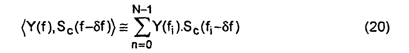
- the continuous dot products of formulas (1) and (3) are therefore naturally replaced by discrete dot products according to relation (2), that is for example:
- the last step of the method is the search for ⁇ f which cancels F ( ⁇ f), or the value "findable” in practice which makes F ( ⁇ f) the closest possible from 0.
- a solution can then be to divide the interval [f max - F e / N, f max + F e / N] into three subintervals [f max - F 0 / N, f max - F e / 3N], [f max - F e / 3N, f max + F e / 3N] and [f max + F e / 3N, f max + F e / N], and perform a dichotomous search in each of the sub-intervals. This ensures that you don't miss the absolute minimum. We also guarantee the convergence of the dichotomous method, for which there must be at most a single zero crossing of the function F to be canceled. Among the three values found for ⁇ f, we retain the one that makes the cost K minimal. For methods other than the dichotomy, which would tolerate the existence of several minima, research could be done on the meeting of the three preceding intervals.
- This fine estimation of ⁇ f is carried out by the synchronization unit 20 in step 37 of FIG. 4. If a digital frequency correction (multiplication of the complex signal not filtered by e -2j ⁇ f ) is provided upstream of the filter 19, this can be performed on the current signal window in order to optimize the representativeness of the baseband signal r n (step 38 of FIG. 4). Otherwise (case illustrated by FIG. 3), the estimated value of ⁇ f is taken into account for the following windows by analog rectification of the frequency of the oscillator 18, in order to correct the drifts of this frequency (or that used by l 'transmitter).
- step 39 the unit 20 provides the estimated time offset ⁇ at demodulator 21, in order to align it with the time structure of the frames and symbols.
- step 40 the unit 20 provides the frequency offset estimated ⁇ f to the oscillator 18 control circuits, so that they correct the deviation with the frequency used by the transmitter.
- Another solution would be to not correct the frequency of the oscillator only if the current estimate of ⁇ f exceeds a determined threshold after the last application of the correction. This allows a correction fast from a large initial deviation.
Abstract
Description
La présente invention concerne le domaine des communications numériques.The present invention relates to the field of communications digital.
On considère un schéma de transmission numérique classique (figure 1) : le signal reçu, consistant en une séquence de symboles, est issu d'un modulateur numérique 1, puis éventuellement déformé par un canal de propagation 2.We consider a classic digital transmission scheme (figure 1): the signal received, consisting of a sequence of symbols, comes from a digital modulator 1, then possibly deformed by a channel spread 2.
Dans de nombreux systèmes, le récepteur 3 nécessite deux informations de synchronisation temporelle : la « date » des frontières entre symboles (pour le fonctionnement du démodulateur), ce qui donne une information de synchronisation modulo la durée d'un symbole ; et une « horloge » système, dont la précision est en nombres entiers de temps symbole, par exemple matérialisée par une frontière entre « trames » si le signal émis possède cette structure (pour bénéficier, par exemple, de la présence de séquences d'apprentissage à des instants précis, et/ou pour savoir où aller décoder ensuite les informations voulues). Cette horloge est indiquée par un ou des symboles particuliers qui jouent le rôle de repères, et que le récepteur doit découvrir.In many systems, the receiver 3 requires two pieces of time synchronization information: the “date” of the borders between symbols (for the operation of the demodulator), which gives synchronization information modulo the duration of a symbol; and a system “clock”, the precision of which is in whole numbers of symbol time, for example materialized by a border between “frames” if the transmitted signal has this structure (to benefit, for example, from the presence of training sequences at specific times, and / or to know where to go and then decode the desired information). This clock is indicated by one or more particular symbols which act as benchmarks, and which the receiver must discover.
De plus, le signal reçu doit être correctement situé dans le domaine fréquentiel, attendu par le démodulateur 4 du récepteur 3. Or, les oscillateurs du récepteur et de l'émetteur ayant une précision limitée, on peut s'attendre à un décalage fréquentiel qu'il convient de corriger.In addition, the received signal must be correctly located in the domain frequency, expected by the demodulator 4 of the receiver 3. However, the oscillators of receiver and transmitter with limited accuracy, we can expect a frequency shift that should be corrected.
L'organe de synchronisation 5 schématisé sur la figure 1 est appelé en
premier par le récepteur. Il délivrera les deux informations (temporelle et
fréquentielle). L'information temporelle sera alors utilisée directement par le
démodulateur / décodeur 4, qui décalera ses références pour atteindre à la fois
la position correcte des symboles ainsi que l'information utile. L'information
fréquentielle sera exploitée par un circuit de correction 6 pour corriger de façon
analogique ou numérique la position fréquentielle du signal reçu. L'organe 5
met en oeuvre un algorithme ayant pour objectif d'estimer le décalage en
fréquence et de retrouver la structure temporelle de l'information.The synchronization member 5 shown diagrammatically in FIG. 1 is called
first by the receiver. It will deliver the two information (temporal and
frequency). The time information will then be used directly by the
demodulator / decoder 4, which will shift its references to reach both
the correct position of the symbols as well as the useful information. information
frequency will be exploited by a
Le premier critère important de performance de la synchronisation est la fiabilité des informations temporelle et fréquentielle obtenues. Un second critère est le coût nécessaire pour obtenir ces informations (temps d'exécution, mémoire et de puissance de calcul nécessaires). Il existe plusieurs familles de méthodes de synchronisation :
- les méthodes en aveugle, couramment appelées NDA (« Non Data Aided »), qui ne nécessitent pas la connaissance par le récepteur d'une partie de l'information transmise (grâce à l'utilisation de propriétés du signal émis, le plus souvent). La plupart de ces méthodes, que ce soit pour estimer l'écart fréquentiel ou temporel, reposent sur le passage du signal par des non-linéarités qui provoquent des raies grâce auxquelles on peut se synchroniser (voir J.B. Anderson et al., « Digital Phase Modulation », Plenum Press, 1986). D'ailleurs, on trouve toute une famille de solutions analogiques (PLL, boucle de Costas, ..., voir J.C. Bic et al., « Eléments de communications numériques », Tome 1, Collection CNET/ENST, Dunod, 1986). L'inconvénient est que ces techniques sont spécialisées par type de modulation, et ne donnent pas d'horloge système d'un niveau plus élevé que le temps symbole ;
- pour la synchronisation système, des solutions à base de codes (notamment de codes convolutifs) ayant des propriétés intéressantes d'autocorrélation. Ceci nécessite bien entendu une synchronisation préalable fréquentielle et temporelle au niveau symbole.
- les méthodes sur trame connue (DA, « Data Aided »), où le récepteur connaít tout ou partie d'une trame permettant d'estimer les informations de synchronisation. Dans le cas du système de radiocommunication cellulaire GSM, une fréquence particulière, c'est-à-dire un signal purement sinusoïdal, sert pour la synchronisation fréquentielle, puis une séquence dédiée (burst) permet la synchronisation temporelle. Un autre exemple est décrit dans FR-A-2 745 134.
- blind methods, commonly called NDA (“ Non Data Aided ”), which do not require the receiver to know part of the information transmitted (most often through the use of properties of the transmitted signal) . Most of these methods, whether to estimate the frequency or time difference, rely on the signal passing through non-linearities which cause lines through which we can synchronize (see JB Anderson et al., "Digital Phase Modulation ”, Plenum Press, 1986). Moreover, there is a whole family of analog solutions (PLL, Costas loop, ..., see JC Bic et al., "Elements of digital communications", Volume 1, Collection CNET / ENST, Dunod, 1986). The disadvantage is that these techniques are specialized by type of modulation, and do not give a system clock of a level higher than the symbol time;
- for system synchronization, solutions based on codes (in particular convolutional codes) having advantageous autocorrelation properties. This of course requires prior frequency and time synchronization at the symbol level.
- methods on known frame (DA, " Data Aided"), where the receiver knows all or part of a frame for estimating synchronization information. In the case of the GSM cellular radiocommunication system, a particular frequency, that is to say a purely sinusoidal signal, is used for frequency synchronization, then a dedicated sequence (burst) allows time synchronization. Another example is described in FR-A-2 745 134.
Les méthodes DA présentent l'inconvénient de faire baisser le débit utile, puisqu'une partie du signal ne transporte pas d'information à proprement parler. Il faut toutefois noter que les méthodes NDA ne sont pas toujours applicables selon la nature du signal, c'est-à-dire du codeur à l'émission. Les méthodes sont alors très spécifiques. Il existe notamment de nombreuses méthodes (voir par exemple : A. D'Andrea et al., « A Digital Approach to Clock Recovery in Generalized Minimum Shift Keying », IEEE Transactions on Vehicular Technology, Vol. 39, No. 3, août 1990 ; A. D'Andrea et al., « frequency Detectors for CPM Signals », IEEE Transactions on Communications, Vol. 43, No. 2-3-4, février/mars/avril 1995) applicables lorsque le codeur est un modulateur CPM (« Continuous Phase Modulation »), qui ne s'appliquent pas aux autres types de modulation. En outre, leurs performances en matière de temps d'exécution, mesurées par la durée pour aboutir aux informations fiables de synchronisation, sont parfois médiocres. Les méthodes DA peuvent se révéler plus efficaces en termes de durée d'exécution, pour une même fiabilité, pour une diminution du débit utile négligeable. De plus, elles sont totalement générales, et ne dépendent pas de la nature du signal utilisé.DA methods have the disadvantage of lowering the useful bit rate, since part of the signal does not carry information properly speaking. However, it should be noted that the NDA methods are not always applicable depending on the nature of the signal, that is to say the coder on transmission. The methods are then very specific. There are many methods in particular (see, for example: A. D'Andrea et al., "A Digital Approach to Clock Recovery in Generalized Minimum Shift Keying", IEEE Transactions on Vehicular Technology, Vol. 39, No. 3, August 1990 ; A. D'Andrea et al., “Frequency Detectors for CPM Signals”, IEEE Transactions on Communications, Vol. 43, No. 2-3-4, February / March / April 1995) applicable when the coder is a CPM modulator (“ Continuous Phase Modulation ”), which do not apply to other types of modulation. In addition, their performance in terms of execution time, measured by time to arrive at reliable synchronization information, is sometimes poor. DA methods can be more effective in terms of execution time, for the same reliability, for a negligible reduction in useful throughput. In addition, they are completely general, and do not depend on the nature of the signal used.
Il existe donc un besoin pour un processus de synchronisation délivrant, dans un laps de temps relativement court, les informations de position temporelle et fréquentielle de l'information. Ce processus doit fonctionner pour des décalages fréquentiels et/ou temporels relativement élevés, dans la limite de la bande utile et pour n'impcrte quel temps d'arrivée du signal utile. La perte d'information utile liée à la durée d'exécution de la synchronisation et/ou à l'insertion de données connues doit être négligeable par rapport au débit utile. De plus, il est souhaitable que ce processus ne soit pas trop coûteux en temps de calcul, et fasse donc essentiellement intervenir des opérations simples (additions, multiplications).There is therefore a need for a synchronization process delivering, in a relatively short period of time, the information of time and frequency position of the information. This process should operate for relatively frequent and / or time offsets high, within the useful band limit and for any arrival time of the useful signal. The loss of useful information related to the duration of execution of the synchronization and / or insertion of known data must be negligible compared to the useful flow. In addition, it is desirable that this process is not not too costly in computation time, and therefore essentially involves simple operations (additions, multiplications).
La méthode habituelle pour acquérir la synchronisation fréquentielle dans le cas de modulations CPM d'indice k/p (J.B. Anderson et al., « Digital Phase Modulation », Plenum Press, 1986) est une méthode en aveugle (NDA) consistant à calculer la transformée de Fourier du signal reçu en bande de base élevé à la puissance p, et à détecter des raies dans le spectre ainsi obtenu. Des raies de fréquence Δf + i/(2Ts) apparaissent en principe dans ce spectre, Δf étant l'écart de fréquence à estimer, Ts la durée d'un symbole et i un entier. Mais leur détection est parfois problématique : elles peuvent être noyées dans la densité spectrale de puissance du signal à la puissance p ou dans le bruit capté par le récepteur, et il peut y avoir une incertitude sur l'entier i valable pour une raie détectée. Ceci dépend des caractéristiques de la CPM employée : les méthodes NDA sont parfois inutilisables.The usual method for acquiring frequency synchronization in the case of CPM modulations of index k / p (JB Anderson et al., "Digital Phase Modulation", Plenum Press, 1986) is a blind method (NDA) consisting in calculating the Fourier transform of the received signal in baseband raised to the power p, and to detect lines in the spectrum thus obtained. Frequency lines Δf + i / (2T s ) appear in principle in this spectrum, Δf being the frequency difference to be estimated, T s the duration of a symbol and i an integer. But their detection is sometimes problematic: they can be embedded in the power spectral density of the signal at power p or in the noise picked up by the receiver, and there can be an uncertainty over the integer i valid for a detected line. This depends on the characteristics of the CPM used: the NDA methods are sometimes unusable.
La présente invention a pour but de répondre au besoin précité, particulièrement en ce qui concerne les aspects de synchronisation fréquentielle. Les applications visées sont notamment les récepteurs de communications numériques nécessitant un organe de synchronisation pour amorcer le décodage de l'information, et pour lesquels les méthodes NDA sont impossibles ou peu performantes. The aim of the present invention is to meet the above-mentioned need, particularly with regard to the timing aspects frequency. The targeted applications are in particular the receivers of digital communications requiring a synchronization device to initiate the decoding of the information, and for which the NDA methods are impossible or poorly performing.
Selon l'invention, il est proposé un procédé de synchronisation d'un
récepteur de communication, dans lequel on évalue un écart entre une
fréquence de modulation, combinée à un premier signal en bande de base
pour former un signal émis sur un canal de propagation et une fréquence
employée par le récepteur pour former un second signal en bande de base à
partir d'un signal reçu sur le canal de propagation, et on corrige la fréquence
employée par le récepteur en fonction de l'écart évalué. Connaissant un
segment temporel du premier signal en bande de base et la position temporelle
d'un segment correspondant du second signal en bande de base, lesdits
segments comprenant N échantillons à une fréquence d'échantillonnage Fe, on
calcule une transformée en fréquence Y(f), de taille N, du produit du complexe
conjugué dudit segment du premier signal en bande de base par le segment
correspondant du second signal en bande de base, et on évalue ledit écart de
fréquence Δf comme étant celui pour lequel la transformée en fréquence Y(f)
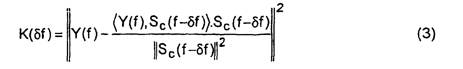
est la plus proche de C.Sc(f-Δf), où Sc(f) est la fonction
Dans une réalisation particulière, l'évaluation de l'écart de fréquence comprend :
- la détermination d'une fréquence fmax qui maximise la quantité |Y(f)|2 parmi les N points de la transformée en fréquence, |.| désignant le module d'un nombre complexe ;
- une division de l'intervalle [fmax - Fe /N, fmax + Fe /N] en plusieurs sous-intervalles ;
- une recherche dichotomique dans chacun des sous-intervalles pour
identifier chaque fréquence δf qui annule la quantité :
où Re(.) et (.)* désignent respectivement la partie réelle et le conjugué d'un nombre complexe et, pour deux fonctions complexes de la fréquence A(f) et B(f), 〈A(f),B(f-δf)〉 désigne le produit scalaire :
 fi désignant le point de rang i de la transformée en fréquence ; et
- la sélection de l'écart de fréquence Δf comme étant celle des fréquences
δf qui annule la quantité F(δf) et pour laquelle la fonction coût :
est minimale, ∥.∥ étant la norme associée audit produit scalaire.
- the determination of a frequency f max which maximizes the quantity | Y (f) | 2 among the N points of the frequency transform, |. | designating the module of a complex number;
- dividing the interval [f max - F e / N, f max + F e / N] into several subintervals;
- a dichotomous search in each of the sub-intervals to identify each frequency δf which cancels the quantity: where Re (.) and (.) * respectively denote the real part and the conjugate of a complex number and, for two complex functions of the frequency A (f) and B (f), 〈A (f), B ( f-δf)〉 denotes the dot product:f i designating the point of rank i of the frequency transform; and
- selecting the frequency deviation Δf as being that of the frequencies δf which cancels the quantity F (δf) and for which the cost function: is minimal, ∥.∥ being the norm associated with said scalar product.
Ledit segment temporel du premier signal en bande de base peut ne pas être connu a priori par le récepteur. Lorsque le récepteur est synchronisé en temps et en fréquence et que l'on souhaite remettre à jour la synchronisation fréquentielle pour corriger éventuellement une légère dérive de l'oscillateur local, on peut ainsi utiliser le résultat de la démodulation et/ou du décodage en tant que « segment temporel du premier signal en bande de base » pour la mise en oeuvre du procédé.Said time segment of the first baseband signal may not not be known a priori by the receiver. When the receiver is synchronized in time and frequency and that we wish to update the frequency synchronization to possibly correct a slight drift of the local oscillator, we can use the result of the demodulation and / or the decoding as a "time segment of the first band signal basis ”for the implementation of the method.
Bien souvent, ledit segment temporel du premier signal en bande de base sera toutefois connu a priori par le récepteur, le procédé comprenant une phase de synchronisation temporelle pour obtenir la position temporelle dudit segment du second signal en bande de base.Very often, said time segment of the first band signal base will however be known a priori by the receiver, the method comprising a time synchronization phase to obtain the time position of said segment of the second baseband signal.
La synchronisation fréquentielle exploite alors des segments de signal requis pour la synchronisation temporelle, ce qui permet de pallier les insuffisances des méthodes NDA généralement employées. Ces segments peuvent rester de taille modérée de sorte que la mise en oeuvre du procédé n'affecte pas trop la bande passante. Cette taille est égale ou supérieure au nombre N précité. La synchronisation fréquentielle est alors conditionnée par la réussite de la synchronisation temporelle, ce qui est peu pénalisant si la probabilité de réussite de la synchronisation temporelle est élevée.Frequency synchronization then uses signal segments required for time synchronization, which overcomes the shortcomings of the NDA methods generally used. These segments may remain of moderate size so that the implementation of the process does not affect bandwidth too much. This size is equal to or greater than number N above. Frequency synchronization is then conditioned by the successful time synchronization, which is not very detrimental if the probability of successful time synchronization is high.
Dans une réalisation préférée, le segment temporel connu a priori comprend plusieurs occurrences consécutives d'un premier motif de Lc échantillons, et éventuellement un second motif plus long que le premier . La phase de synchronisation temporelle comprend une étape de d'estimation modulo Lc par maximisation de la corrélation entre le second signal en bande de base et les occurrences consécutives du premier motif, et une étape de levée d'ambiguïté du modulo Lc, fournissant une synchronisation temporelle à la résolution des échantillons par maximisation de la corrélation entre le second signal en bande de base et le second motif.In a preferred embodiment, the time segment known a priori comprises several consecutive occurrences of a first pattern of L c samples, and possibly a second pattern longer than the first. The time synchronization phase comprises a step of modulo L c estimation by maximizing the correlation between the second baseband signal and the consecutive occurrences of the first pattern, and a step of removing ambiguity from the modulo L c , providing time synchronization at the resolution of the samples by maximizing the correlation between the second baseband signal and the second pattern.
Après avoir ainsi réalisé une première synchronisation temporelle
produisant un nombre entier nest représentant un décalage temporel, en
nombre d'échantillons, du second signal en bande de base par rapport audit
segment temporel du premier signal en bande de base, on affine la première
synchronisation temporelle en ajoutant au nombre entier nest la quantité :


Un autre aspect de la présente invention se rapporte à un dispositif de synchronisation d'un récepteur de communication, comprenant des moyens d'analyse d'un signal reçu, agencés pour mettre en oeuvre un procédé tel que défini ci-dessus.Another aspect of the present invention relates to a device for synchronization of a communication receiver, comprising means analysis of a received signal, arranged to implement a method such as defined above.
D'autres particularités et avantages de la présente invention apparaítront dans la description ci-après d'exemples de réalisation non limitatifs, en référence aux dessins annexés, dans lesquels :
- la figure 1, précédemment commentée, est un schéma synoptique d'une chaíne de transmission numérique ;
- la figure 2 montre un exemple de réalisation d'un modulateur d'un émetteur radio numérique ;
- la figure 3 est un schéma synoptique d'un récepteur associé, ayant un module de synchronisation pour la mise en oeuvre de l'invention ; et
- la figure 4 est un organigramme d'une procédure mise en oeuvre par ce module de synchronisation.
- Figure 1, previously commented, is a block diagram of a digital transmission chain;
- FIG. 2 shows an exemplary embodiment of a modulator of a digital radio transmitter;
- FIG. 3 is a block diagram of an associated receiver, having a synchronization module for implementing the invention; and
- FIG. 4 is a flow diagram of a procedure implemented by this synchronization module.
L'invention est illustrée ci-après dans une application particulière aux radiocommunications avec des terminaux mobiles. On comprendra que cet exemple ne limite aucunement le champ d'application de l'invention.The invention is illustrated below in a particular application to radiocommunications with mobile terminals. We will understand that this example in no way limits the scope of the invention.
Dans cet exemple particulier, l'information transmise est découpée en
trames de 20 ms. Le modulateur numérique représenté sur la figure 2
fonctionne selon une modulation de type CPM quaternaire, d'indice de
modulation 1/3, dont l'impulsion de phase
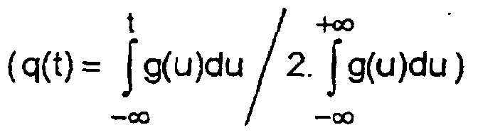

Cette modulation CPM peut être décrite par un treillis comportant 3 états de phase (0, 2π/3 , -2π/3 aux temps-symbole pairs, et π, -π/3, π/3 aux temps-symbole impairs) et 4 transitions par état (correspondant aux quatre symboles possibles).This CPM modulation can be described by a trellis comprising 3 phase states (0, 2π / 3, -2π / 3 at even symbol times, and π, -π / 3, π / 3 at odd time symbol) and 4 transitions per state (corresponding to the four possible symbols).
Dans la réalisation montrée sur la figure 2, le filtre 10 applique
l'impulsion de phase q(t) au train de symboles αi. Les cosinus et sinus de la
phase résultante ϕ(t), formant respectivement les parties réelle et imaginaire du
signal en bande de base x(t), sont fournis par un module 11, échantillonnés à
une fréquence Fe = 16 KHz (deux échantillons complexes par temps-symbole).In the embodiment shown in FIG. 2, the
Deux multiplieurs 12 modulent respectivement deux ondes radio en
quadrature de fréquence f0, délivrées par un oscillateur local 13, par les parties
réelle et imaginaire du signal en bande de base x(t) converties en analogique.
Les deux ondes modulées sont sommées en 14 pour former le signal radio
amplifié et émis par l'antenne 15.Two
Le canal de propagation 2 associé est un canal à évanouissements, dit canal de Rayleigh. Le démodulateur utilisé par le récepteur de la figure 3 peut reposer sur un algorithme de Viterbi classique fonctionnant selon le treillis précité (voir G. D. Fomey Jr., « The Viterbi Algorithm », Proc. of the IEEE, Vol. 61, No. 3, mars 1973, pages 268-278). Ce démodulateur nécessite d'être synchronisé temporellement et fréquentiellement.The associated propagation channel 2 is a fading channel, known as Rayleigh canal. The demodulator used by the receiver of FIG. 3 can be based on a classical Viterbi algorithm operating according to the trellis cited above (see G. D. Fomey Jr., "The Viterbi Algorithm", Proc. of the IEEE, Vol. 61, No. 3, March 1973, pages 268-278). This receiver needs to be time and frequency synchronized.
Le signal radio reçu par l'antenne 16 et amplifié est soumis à deux
multiplieurs 17 recevant deux ondes en quadrature de fréquence f0 + Δf,
délivrées par un oscillateur local 18. Les sorties des multiplieurs 17 forment un
signal complexe traité par un filtre passe-bas 19, dont la fréquence de coupure
correspond à la bande utile du signal, par exemple 6 kHz. Le signal complexe
en bande de base r(t) disponible en sortie du filtre 19 est échantillonné à la
fréquence Fe et numérisé, en aval ou en amont du filtre 19 selon que celui-ci
est réalisé sous forme analogique ou numérique. On note rn ce signal en
bande de base échantillonné, n étant l'index des échantillons. Le signal
numérique rn est adressé à une unité de synchronisation 20 et au
démodulateur 21 qui produira les estimations α andi des symboles transmis.The radio signal received by the
Le décalage fréquentiel Δf peut être dû aux imprécisions de l'oscillateur
local 13 de l'émetteur et/ou de celui 18 du récepteur. Il existe d'autre part un
décalage temporel τ entre l'émetteur et le récepteur, dû au temps de
propagation inconnu. Le signal en bande de base r(t) obtenu dans l'étage radio
du récepteur peut être exprimé en fonction de celui x(t) formé par l'émetteur :
On suppose que dans l'exemple considéré, le décalage temporel τ est limité en valeur absolue à 10 ms, et que le décalage fréquentiel Δf ne peut dépasser, toujours en valeur absolue, 5 kHz.We assume that in the example considered, the time shift τ is limited in absolute value to 10 ms, and that the frequency offset Δf cannot exceed, always in absolute value, 5 kHz.
Si le décalage fréquentiel Δf est excessif (proche de sa valeur limite), on perd une part importante de l'énergie utile en raison du filtrage opéré en 19. II est alors nécessaire d'effectuer une première synchronisation fréquentielle grossière permettant de réduire ce décalage.If the frequency offset Δf is excessive (close to its limit value), a significant part of the useful energy is lost due to the filtering carried out in 19. It is then necessary to carry out a first frequency synchronization coarse to reduce this lag.
Le récepteur ne peut couvrir une bande fréquentielle infinie ; celle-ci est limitée par des considérations matérielles (bande passante des composants) et peut être intentionnellement sélectionnée par des dispositifs de filtrage. En particulier, dans un système fonctionnant en accès multiple à répartition en fréquence (FDMA), on sélectionne le canal fréquentiel correspondant à la communication souhaitée. Cette restriction du domaine fréquentiel est effectuée dans le premier étage du récepteur (filtre 19 dans l'exemple représenté).The receiver cannot cover an infinite frequency band; this one is limited by hardware considerations (bandwidth of components) and can be intentionally selected by filtering. In particular, in a system operating in multiple access to frequency distribution (FDMA), select the frequency channel corresponding to the desired communication. This domain restriction frequency is carried out in the first stage of the receiver (filter 19 in the example shown).
Qu'elle soit volontaire ou non, cette sélection fréquentielle peut avoir des conséquences néfastes sur les traitements du signal rn obtenu après ce premier étage. En effet, l'oscillateur générant la fréquence porteuse supposée présente une certaine imprécision, et la fréquence porteuse réelle du signal et celle utilisée par le récepteur ne peuvent être rigoureusement identiques. Si elles sont éloignées, le filtrage autour de la porteuse utilisée par le récepteur peut alors entraíner l'élimination d'une partie de l'énergie du signal utile, qui sera perdue pour les traitements ultérieurs.Whether voluntary or not, this frequency selection can have harmful consequences on the processing of the signal r n obtained after this first stage. Indeed, the oscillator generating the supposed carrier frequency has a certain imprecision, and the real carrier frequency of the signal and that used by the receiver cannot be strictly identical. If they are distant, the filtering around the carrier used by the receiver can then result in the elimination of part of the energy of the useful signal, which will be lost for subsequent processing.
On note cependant que les incertitudes sur les fréquences générées
par les oscillateurs 13, 18 sont maítrisables, et qu'on connaít souvent la valeur
maximale possible pour le décalage entre la fréquence souhaitée et celle
réellement modulée (5 kHz dans l'exemple considéré). Il demeure que ce
décalage, s'il n'est pas négligeable devant la bande utile du signal transmis,
peut affecter ce dernier d'une façon irrémédiable. La première synchronisation
fréquentielle proposée vise à corriger grossièrement le décalage fréquentiel
initial, pour le ramener à une valeur beaucoup plus faible.Note however that the uncertainties on the frequencies generated
by
Ce premier traitement est composé d'une estimation grossière du décalage fréquentiel et d'une correction réalisée dans le premier étage du récepteur, en analogique ou en numérique. Cette estimation offre l'intérêt d'être robuste aux forts décalages fréquentiels, même lorsqu'une grande partie de l'énergie du signal a disparu à cause du filtrage du récepteur.This first treatment consists of a rough estimate of the frequency shift and a correction made in the first floor of the receiver, analog or digital. This estimate offers the advantage of being robust at high frequency shifts, even when a large part of the signal energy has disappeared due to the filtering of the receiver.
La fenêtre de signal numérique observé rn de longueur Lr (n = 0, ...,
Lr-1) est le résultat de la transmission d'un signal xn, inconnu du récepteur,
bruité et déformé par le canal de propagation 2. La formule suivante donne une
première estimation du décalage fréquentiel :

En effet, si le signal reçu est simplement le signal xn décalé
fréquentiellement de Δf, la formule (7) donne bien Δf1= Δf. On note qu'un
décalage temporel sur xn n'a aucune influence sur l'estimation Δf1. La quantité

De plus, pour de nombreux types de signaux, en particulier les
modulations CPM comme dans l'exemple ci-dessus, l'autocorrélation est réelle,
et l'expression de Δf1 ne dépend plus que du signal reçu rn (voir A. D'Andrea et
al., « Digital Carrier Frequency Estimation For Multilevel CPM Signals »,
Proc. ICC'95, juin 1995). L'estimation grossière Δf1 est alors simplement :

Cette estimation est effectuée par l'unité de synchronisation 20 à
l'étape 30 de la figure 4. Si une correction de fréquence numérique, à savoir
une multiplication du signal complexe non filtré par e-2jπΔf 1, est prévue en
amont du filtre 19, celle-ci peut être effectuée sur la fenêtre de signal courante
en vue des traitements suivants (étape 31 de la figure 4). Sinon (cas illustré par
la figure 3), les autres traitements de synchronisation sont effectués sans
correction de fréquence grossière, et celle-ci sera (éventuellement) prise en
compte pour les fenêtres suivantes par rectification analogique de la fréquence
de l'oscillateur 18 (étape 40).This estimation is carried out by the
Des simulations ont montré que, dans l'exemple considéré, quelles que soient les conditions de propagation, et pour des décalages fréquentiels initiaux dans [-5, +5] kHz, le décalage résiduel après cette correction grossière n'est jamais supérieur à 1500 Hz.Simulations have shown that, in the example considered, whatever are the propagation conditions, and for initial frequency shifts in [-5, +5] kHz, the residual offset after this coarse correction is not never higher than 1500 Hz.
Après la correction fréquentielle grossière, le décalage fréquentiel résiduel est beaucoup moins élevé, ce qui permet la synchronisation temporelle et fréquentielle fine décrite ci-dessous.After the coarse frequency correction, the frequency shift residual is much lower, which allows synchronization fine time and frequency described below.
La trame de synchronisation choisie dans l'exemple est un segment de
référence de 10 ms inséré dans le flot des trames utiles, toutes les 500 ms. A
chaque début de communication, l'unité 20 du récepteur lance l'algorithme de
synchronisation qui s'arrête une fois la trame de synchronisation détectée et le
traitement effectué.The synchronization frame chosen in the example is a segment of
10 ms reference inserted in the flow of useful frames, every 500 ms. AT
at the start of communication, the
Le segment de référence utilisé, d'une durée de 10 ms, est composé dans l'exemple considéré de Nc = 3 motifs courts, identiques et consécutifs, de 16 symboles chacun puis d'un motif long de 32 symboles. Le motif court correspond par exemple à la modulation de la suite de 16 symboles : {-3, -3, +1, -1, +1, +1, +1, -3, +1, -3, +3, +1, -3, -3, +3, +3}. Ce motif est donc composé de Lc = 32 échantillons prédéterminés. On note x c / k la séquence répétitive de ces échantillons (0 ≤ k < LSc = Nc.Lc = 96).The reference segment used, with a duration of 10 ms, is composed in the example considered of N c = 3 short patterns, identical and consecutive, of 16 symbols each then of a long pattern of 32 symbols. The short pattern corresponds for example to the modulation of the sequence of 16 symbols: {-3, -3, +1, -1, +1, +1, +1, -3, +1, -3, +3, +1, -3, -3, +3, +3}. This pattern is therefore composed of L c = 32 predetermined samples. We denote by xc / k the repetitive sequence of these samples (0 ≤ k <L Sc = N c .L c = 96).
Le motif long correspond par exemple à la modulation de la suite de 32 symboles : {+3, -1, +1, +1, +1, -3, -3, -3, -3, -3, -1, -3, +1, +3, +3, -1, +1, +3, -3, -3, +3, +3, +3, +1, +3, -3, -3, +1, -1, +1, +1, -3}. Il est donc composé de Ll = 64 échantillons prédéterminés. On note x l / k la suite de ces échantillons (0 ≤ k < Ll).The long pattern corresponds for example to the modulation of the sequence of 32 symbols: {+3, -1, +1, +1, +1, -3, -3, -3, -3, -3, -1, -3, +1, +3, +3, -1, +1, +3, -3, -3, +3, +3, +3, +1, +3, -3, -3, +1 , -1, +1, +1, -3}. It is therefore composed of L l = 64 predetermined samples. We denote by xl / k the sequence of these samples (0 ≤ k <L l ).
On note enfin xk la suite des N' = LSc + Ll = 160 échantillons correspondant au segment de référence de 10 ms (xk =x c / k si k < LSc, xk =x l / k-LSc si LSc ≤ k < N').We finally note x k the sequence of N '= L Sc + L l = 160 samples corresponding to the reference segment of 10 ms (x k = xc / k if k <L Sc , x k = xl / kL Sc if L Sc ≤ k <N ').
L'algorithme de synchronisation temporelle comporte trois étapes :
- un test de répétition pour tester la présence d'une zone répétitive correspondant à la succession de motifs courts ;
- un calcul de corrélation avec le motif court, pour estimer le décalage τ modulo Lc, suivi par un calcul de corrélation avec le motif long aux positions correspondant à la première estimation modulo Lc. Ce calcul donne l'estimation de « l'horloge système » et une information sur la vraisemblance de cette estimée ;
- une estimation fine procurant une résolution temporelle plus fine que Te = 1/Fe pour le décalage temporel τ.
- a repetition test for testing the presence of a repeating zone corresponding to the succession of short patterns;
- a correlation calculation with the short pattern, to estimate the shift τ modulo L c , followed by a correlation calculation with the long pattern at the positions corresponding to the first modulo estimate L c . This calculation gives the estimate of the “system clock” and information on the likelihood of this estimate;
- a fine estimate providing a finer time resolution than T e = 1 / F e for the time shift τ.
Ce test 32 permet de s'assurer de la nature de la trame qu'on traite. En
effet, selon la valeur du décalage temporel et la mémoire disponible en
réception, le signal observé peut ne pas contenir la trame de synchronisation.
On peut alors utiliser la structure répétitive de la trame de synchronisation pour
la reconnaítre (l'information étant par hypothèse aléatoire et donc peu
répétitive), et ainsi interrompre l'algorithme dès ce premier test si celui-ci n'est
pas concluant. Ceci permet de diminuer la quantité moyenne de calculs à
effectuer.This
Le test 32 consiste à évaluer une autocorrélation normalisée du signal
en bande de base rn relativement à un décalage temporel correspondant au
décalage Lc entre deux occurrences du motif court xc dans le segment de
référence.
Pour reconnaítre la trame de synchronisation, on effectue un calcul de
répétition sur Lc échantillons jusqu'à ce qu'on dépasse un seuil SR (par
exemple SR ≈ 0,25). On calcule ainsi l'indicateur suivant, pour 1 ≤ m < Lr/Lc :

Si le seuil SR n'est jamais atteint par rep(m) sur la longueur du signal
mémorisé (test 32 de la figure 4), la synchronisation échoue, et l'unité de
synchronisation 20 commande simplement l'oscillateur 18 pour qu'il prenne en
compte (éventuellement) la correction de fréquence représentée par
l'estimation grossière Δf1 pour la prochaine fenêtre d'observation du signal
(étape 40). Si le test de répétition est satisfait, l'unité 20 recherche le segment
de synchronisation.If the threshold SR is never reached by rep (m) over the length of the memorized signal (
On choisit une taille de fenêtre d'observation Lr telle qu'on soit assuré de pouvoir acquérir entièrement la trame de synchronisation. Une solution préférée est une fenêtre de taille 2 fois celle du motif total de synchronisation, soit 20 ms ou Lr = 320, dont la première moitié est la même que la seconde moitié de la fenêtre précédente, et dont la seconde moitié est la même que la première moitié de la fenêtre suivante. Le test de répétition sert alors uniquement à éviter le lancement intempestif de l'algorithme.We choose an observation window size L r such that we can be sure that we can fully acquire the synchronization frame. A preferred solution is a window twice the size of the total synchronization pattern, i.e. 20 ms or L r = 320, the first half of which is the same as the second half of the previous window, and the second half of which is the same than the first half of the next window. The repetition test is then only used to avoid untimely launching of the algorithm.
On recherche d'abord le motif court sur toute la longueur du signal
observé, en se décalant progressivement de n = 0, 1, ... , Lc-1 échantillons, et
de m fois la longueur d'un motif court (m = 0, 1, 2, ... ) jusqu'à ce que la fin de
la zone de mémoire accessible soit atteinte. Cette recherche est effectuée
grâce à un calcul de corrélations entre la portion de signal considérée et la
partie du segment de référence correspondant à la succession de motifs
courts. La corrélation C(n,m), indexée par n et m avec 0 ≤ n < Lc et
0 ≤ m < Lr/Lc, est calculée à l'étape 33 selon :
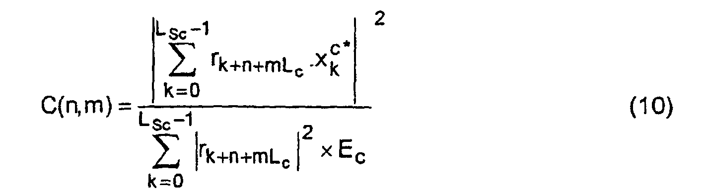
La corrélation est normalisée par le produit des énergies du signal reçu
et du signal
![]()
![]()
![]()
![]()
On cherche à présent une approximation du décalage en nombre
d'entiers d'échantillons. Les décalages possibles sont donc de la forme
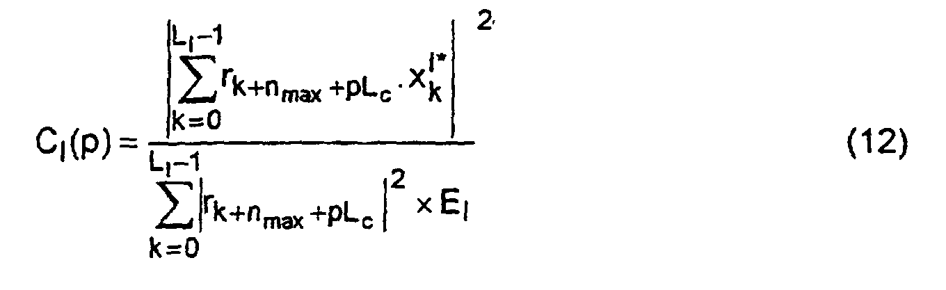
nmax + p.Lc, où p est un entier positif ou nul. On teste donc ces positions en
calculant, à l'étape 34, les corrélations entre le motif long xl et le signal à partir
de ces points, pour 0 ≤ p < Lr/Lc :

![]()
![]()
A l'étape 34, l'unité de synchronisation 20 déduit le décalage temporel
cherché τ, exprimé en nombre d'échantillons, de la position du motif long, en
supprimant la partie correspondant aux motifs courts :
On peut ajouter à cette estimation une information supplémentaire : la qualité de la synchronisation, qui est définie comme le maximum Q = Cl(pmax) des modules des corrélations Cl(p). L'information de qualité Q se rapporte la vraisemblance de l'estimée.We can add to this estimate additional information: the quality of synchronization, which is defined as the maximum Q = C l (p max ) of the correlation modules C l (p). The quality information Q relates to the likelihood of the estimate.
Ceci procure un test pour juger de la fiabilité du processus de
synchronisation : si la qualité Q n'est pas supérieure à un seuil donné SQ, on
peut décider que la synchronisation a échoué sur la fenêtre de signal courante,
et de recommencer le processus de synchronisation sur une autre observée. A
titre d'exemple, on peut prendre SQ ≈ 0,35. Ce test est effectué à l'étape 35 de
la figure 4. S'il n'est pas satisfait (Q < SQ), la synchronisation échoue, et l'unité
de synchronisation 20 commande simplement l'oscillateur 18 pour qu'il prenne
(éventuellement) en compte la correction de fréquence représentée par
l'estimation grossière Δf1 pour la prochaine fenêtre d'observation du signal
(étape 40). Sinon, l'unité 20 passe aux phases suivantes du procédé, dans
lesquelles elle affine la synchronisation.This provides a test to judge the reliability of the synchronization process: if the quality Q is not greater than a given threshold SQ, it can be decided that synchronization has failed on the current signal window, and to start again the process of synchronization on another observed. As an example, we can take SQ ≈ 0.35. This test is carried out in
Lorsque le décalage temporel τ est limité pour des considérations matérielles à une valeur τmax faible devant la durée d'un symbole, il est à noter que le segment de référence peut se composer seulement d'une succession de motifs courts de durée égale ou supérieure à τmax. La levée de l'ambiguïté de la longueur du motif court n'est alors plus nécessaire. En outre, on peut alors utiliser un grand nombre de motifs courts, ce qui permet d'améliorer la précision de la synchronisation temporelle fine exposée ci-après.When the time offset τ is limited for material considerations to a value τ max small compared to the duration of a symbol, it should be noted that the reference segment can consist only of a succession of short patterns of equal or greater duration at τ max . The ambiguity of the length of the short pattern is no longer necessary. In addition, a large number of short patterns can then be used, which makes it possible to improve the precision of the fine time synchronization described below.
La valeur précédente nest est une approximation du décalage τ en nombre d'échantillons. La précision de l'estimation peut être augmentée grâce à un calcul utilisant la dérivée du signal de référence. On utilise ici la succession de motifs courts, car le calcul effectué est non-cohérent, et la répétition de ces motifs améliore sensiblement la performance de l'estimation fine.The previous value n is an approximation of the shift τ in number of samples. The precision of the estimate can be increased by means of a calculation using the derivative of the reference signal. The succession of short patterns is used here, since the calculation performed is non-coherent, and the repetition of these patterns significantly improves the performance of the fine estimation.
On note dxc la dérivée numérique du motif court xc, de longueur LSc-1.
La position du début du motif court xc est à présent connue (à une précision
d'un échantillon près). L'unité de synchronisation 20 affine l'estimation de τ à
l'étape 36 en ajoutant à nest la quantité Δτ calculée selon la relation (4) donnée
plus haut, le facteur de normalisation λ de la relation (5) ayant été calculé une
fois pour toutes et mémorisé dans l'unité 20.We denote by dx c the numerical derivative of the short pattern x c , of length L Sc -1. The position of the start of the short pattern x c is now known (to an accuracy of one sample). The
On note que l'éventuel décalage en fréquence résiduel n'a pas
d'influence sur le calcul de Δτ. Ce calcul conduit à estimer le décalage τ en
L'estimation affinée τ permet d'optimiser les performances du
démodulateur de Viterbi 21.The refined estimate τ optimizes the performance of the
On suppose dans la suite que l'unité de synchronisation 20 du
récepteur a préalablement acquis la synchronisation temporelle sur l'émetteur
à la résolution des échantillons (le calcul de nest suffit donc). Le principe de la
synchronisation fréquentielle fine selon l'invention est de multiplier point à point
le signal reçu par le conjugué du signal attendu, convenu entre l'émetteur et le
récepteur, ce qui aura pour effet d'éliminer du résultat la phase de la
modulation. Si de surcroít la modulation est à enveloppe constante, ce résultat
sera simplement une sinusoïde (complexe) noyée dans le bruit du récepteur.
On peut alors estimer la fréquence de cette sinusoïde, qui sera retirée de la
fréquence de l'oscillateur 18 du récepteur, et/ou exploitée dans un traitement
numérique, notamment de correction de fréquence.It is assumed hereinafter that the
Ce procédé fonctionne également dans le cas d'une modulation où l'amplitude n'est pas constante, car au lieu d'avoir une sinusoïde, on a une sinusoïde modulée en amplitude : il y a toujours une raie à la fréquence centrale.This process also works in the case of a modulation where the amplitude is not constant, because instead of having a sinusoid, we have a amplitude modulated sinusoid: there is always a line at the frequency Central.
On emploie ci-après le formalisme habituel des espaces de Hilbert (ici
celui des vecteurs complexes de dimension N), et on utilisera donc le produit
scalaire entre 2 vecteurs x = (x0, x1, ..., xn-1)T et y = (y0, y1, ..., yn-1)T :


Le critère dont va découler la méthode décrite ci-après est celui du maximum de vraisemblance.The criterion from which the method described below will flow is that of maximum likelihood.
Soit N le nombre d'échantillons permettant de représenter le signal reçu. Ce nombre N peut être égal ou inférieur au nombre N' d'échantillons du segment de référence. Pour la mise en oeuvre de la méthode, qui utilise une transformée en fréquence telle qu'une transformée de Fourrier Rapide (TFR), N sera de préférence une puissance de 2, ou du moins une valeur autorisant un calcul commode de TFR. Dans l'exemple considéré, N = 128 convient.Let N be the number of samples used to represent the signal received. This number N can be equal to or less than the number N 'of samples of the reference segment. For the implementation of the method, which uses a frequency transform such as a Fast Fourier transform (TFR), N will preferably be a power of 2, or at least a value authorizing a convenient calculation of TFR. In the example considered, N = 128 is suitable.
On a acquis à ce stade les paramètres de synchronisation temporelle,
de sorte qu'on connaít parfaitement la forme du signal attendu. Le canal de
propagation et l'écart de porteuse restent inconnus. On désigne par
s = (s0, s1, ..., sn-1)T le signal émis en bande de base (x) décalé d'une
fréquence Δf. La densité de probabilité du signal reçu, conditionnellement à
l'émission du signal x, s'écrit :


Dans la suite, on supposera que la modulation employée est à
enveloppe constante (normalisée à 1), et donc le signal s aussi. Par
conséquent, le carré de la norme de s est égal au nombre d'échantillons N, et
l'expression de Θ se simplifie encore :

On peut alors élaborer une stratégie, pour estimer Δf, basée sur une
transformée de Fourier du signal y. L'étape 37 d'estimation fine de Δf
commence donc par le calcul du vecteur y (yn = rn. x*n pour 0 ≤ n < N), et par le
calcul de sa TFD grâce à un algorithme standard de TFR complexe. Ensuite,
l'unité 20 recherche, parmi les fréquences « naturelles » de cette TFR, celle
fmax qui rend le module carré de cette TFR maximum. La TFR est définie en un
nombre N de fréquences, ou points, fi données par fi = i.Fe / N, pour 0 ≤ i < N.We can then develop a strategy, to estimate Δf, based on a Fourier transform of the signal y.
Bien entendu, la recherche du maximum
![]()
![]()
La transformée de Fourier discrète Sc(f) d'une séquence de « 1 » finie
de longueur N a pour module un sinus cardinal :
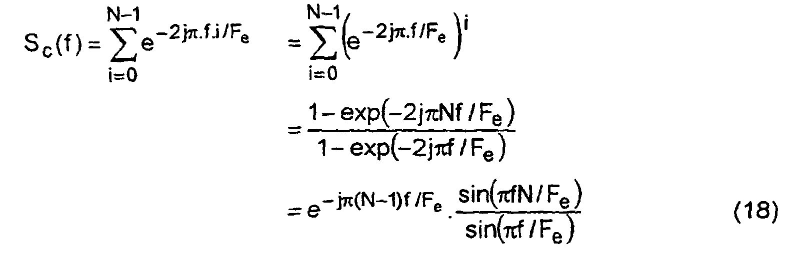
La transformée de Fourier discrète d'un signal tronqué à N échantillons est la convolution de la transformée de Fourier discrète de ce signal non tronqué par la fonction Sc(f).The discrete Fourier transform of a truncated signal with N samples is the convolution of the discrete Fourier transform of this non-truncated signal by the function S c (f).
Le signal y précité est en principe une sinusoïde complexe affectée
d'un coefficient complexe C rendant compte de la propagation, plus du bruit, à
savoir :
On cherche alors C et Δf qui permettent d'approcher Y(f) au mieux par
une fonction C.Sc(f-Δf), au sens des moindres carrés, c'est-à-dire pour
lesquelles le coût K(C,Δf)=∥Y(f)-C.Sc(f-Δf)∥2 est minimum. Par un calcul
similaire à celui présenté plus haut, on trouve que la solution pour C est
Dans l'expression de K et de C, les calculs sont faits dans l'espace des fonctions de carré sommable. En utilisant le fait que la norme de Sc est indépendante de δf, on montre que la valeur optimale Δf annule la fonction F(δf) de la relation (1).In the expression of K and C, the calculations are made in the space of summable square functions. Using the fact that the norm of S c is independent of δf, we show that the optimal value Δf cancels the function F (δf) of the relation (1).
Sur la base du signal reçu rn, l'unité 20 détermine Y(f), échantillonnée
aux fréquences fi. Elle mémorise d'autre part les valeurs de Sc(f-δf) et de sa
dérivée par rapport à δf, échantillonnées avec la résolution souhaitée pour
l'estimation de Δf. Les produits scalaires continus des formules (1 ) et (3) sont
donc naturellement remplacés par des produits scalaires discrets selon la
relation (2), soit par exemple :
La dernière étape de la méthode est la recherche de Δf qui annule F(δf), ou de la valeur « trouvable » en pratique qui rend F(δf) le plus proche possible de 0.The last step of the method is the search for Δf which cancels F (δf), or the value "findable" in practice which makes F (δf) the closest possible from 0.
Une technique possible est une recherche dichotomique sur un ensemble prédéfini de valeurs de δf. On montre que la fonction de coût K(δf) possède, en plus du minimum absolu en Δf, une série de minima locaux distants de Δf de multiples de Fe/N, qui se traduisent par des valeurs nulles de la fonction F. Il faut donc prendre garde à ne pas converger vers un de ces minima locaux. Pour cela, on note que la fréquence naturelle fmax pour laquelle |Y(f)|2 est maximum donne une indication sur la vraie valeur de Δf avec une erreur valant au plus Fe/N (la résolution fréquentielle de la TFR employée). Par conséquent, si on cherche Δf autour de cette première valeur, il y a un risque de trouver une valeur fausse de ± Fe/N par rapport à la vraie valeur (cela dépend de la résolution en fréquence de la TFR et de l'emplacement de fmax par rapport à Δf), mais pas au-delà.One possible technique is a dichotomous search on a predefined set of values of δf. We show that the cost function K (δf) has, in addition to the absolute minimum in Δf, a series of local minima distant from Δf by multiples of F e / N, which result in zero values of the function F. It care must therefore be taken not to converge on one of these local minima. For this, we note that the natural frequency f max for which | Y (f) | 2 is maximum gives an indication of the true value of Δf with an error of at most F e / N (the frequency resolution of the TFR used). Consequently, if we seek Δf around this first value, there is a risk of finding a false value of ± F e / N compared to the true value (it depends on the frequency resolution of the TFR and of the location of f max with respect to Δf), but not beyond.
Une solution peut alors être de diviser l'intervalle [fmax - Fe/N, fmax + Fe/N] en trois sous-intervalles [fmax - F0/N, fmax - Fe/3N], [fmax - Fe/3N, fmax + Fe/3N] et [fmax + Fe/3N, fmax + Fe/N], et d'effectuer une recherche dichotomique dans chacun des sous-intervalles. Ceci assure de ne pas manquer le minimum absolu. On garantit en outre la convergence de la méthode dichotomique, pour laquelle il faut qu'il y ait au plus un seul passage par zéro de la fonction F à annuler. Parmi les trois valeurs trouvées pour Δf, on retient celle qui rend le coût K minimal. Pour méthodes autres que la dichotomie, qui toléreraient l'existence de plusieurs minima, la recherche pourrait se faire sur la réunion des trois intervalles précédents.A solution can then be to divide the interval [f max - F e / N, f max + F e / N] into three subintervals [f max - F 0 / N, f max - F e / 3N], [f max - F e / 3N, f max + F e / 3N] and [f max + F e / 3N, f max + F e / N], and perform a dichotomous search in each of the sub-intervals. This ensures that you don't miss the absolute minimum. We also guarantee the convergence of the dichotomous method, for which there must be at most a single zero crossing of the function F to be canceled. Among the three values found for Δf, we retain the one that makes the cost K minimal. For methods other than the dichotomy, which would tolerate the existence of several minima, research could be done on the meeting of the three preceding intervals.
Cette estimation fine de Δf est effectuée par l'unité de synchronisation
20 à l'étape 37 de la figure 4. Si une correction de fréquence numérique,
(multiplication du signal complexe non filtré par e-2jπΔf), est prévue en amont
du filtre 19, celle-ci peut être effectuée sur la fenêtre de signal courante afin
d'optimiser la représentativité du signal en bande de base rn (étape 38 de la
figure 4). Sinon (cas illustré par la figure 3), la valeur estimée de Δf est prise en
compte pour les fenêtres suivantes par rectification analogique de la fréquence
de l'oscillateur 18, afin de corriger les dérives de cette fréquence (ou de celle
utilisée par l'émetteur).This fine estimation of Δf is carried out by the
A l'étape 39, l'unité 20 fournit le décalage temporel estimé τ au
démodulateur 21, afin de l'aligner sur la structure temporelle des trames et des
symboles.In
Finalement, à l'étape 40, l'unité 20 fournit le décalage fréquentiel
estimé Δf aux circuits de contrôle de l'oscillateur 18, afin qu'ils corrigent l'écart
avec la fréquence employée par l'émetteur.Finally, in
On a mentionné que la correction de la fréquence de l'oscillateur 18
pouvait n'être qu'éventuelle lorsque le segment de référence n'a pas été
détecté (test 32 ou 35). Cette correction ne doit pas être appliquée
systématiquement s'il n'y a pas de garantie que le segment de référence,
lorsqu'il est bien présent, se trouve entièrement dans une fenêtre d'observation
du signal (il peut par exemple se trouver à cheval sur deux fenêtres
consécutives). La correction de fréquence grossière peut donc être
conditionnée lorsque le test 32 ou 35 est négatif. On peut par exemple choisir
de n'effectuer cette correction que périodiquement, avec une fréquence assez
peu élevée afin de laisser plusieurs paquets d'échantillons consécutifs avec le
même écart de fréquence. En choisissant la période et celle de répétition du
segment de référence, exprimées en nombres de trames, de telle sorte qu'elles
soient premières entre elles, on se prémunit contre le cas pathologique où on
appliquerait systématiquement la correction de fréquence pile sur le segment
de signal connu.It has been mentioned that the correction of the frequency of
Une autre solution consisterait à ne corriger la fréquence de l'oscillateur que si l'estimation courante de Δf dépasse un seuil déterminé après la dernière application de la correction. Ceci permet une correction rapide d'un fort écart initial.Another solution would be to not correct the frequency of the oscillator only if the current estimate of Δf exceeds a determined threshold after the last application of the correction. This allows a correction fast from a large initial deviation.
Des simulations ont été effectuées dans le cas de l'exemple numérique donné ci-dessus à titre d'illustration, en prenant en compte trois critères :
- la probabilité de non détection du segment de référence (échec de
l'algorithme au
test 32ou 35 ; - la probabilité de mauvaise synchronisation temporelle, à 0,25 temps symbole près ;
- la probabilité de mauvaise synchronisation fréquentielle, à 50 Hz près.
- the probability of non-detection of the reference segment (failure of the algorithm in
test - the probability of poor time synchronization, to the nearest 0.25 symbol times;
- the probability of bad frequency synchronization, to within 50 Hz.
Le Tableau I montre les résultats obtenus dans deux conditions de simulation :
Claims (11)
- A method of synchronising a communication receiver, comprising the steps of evaluating a deviation between a modulation frequency, combined with a first baseband signal to form a signal transmitted on a propagation channel and a frequency used by the receiver to form a second baseband signal (rn) from a signal received on the propagation channel, and adjusting the frequency used by the receiver according to the evaluated deviation, characterised in that, knowing a time segment of the first baseband signal and the time position of a corresponding segment of the second baseband signal, said segments comprising N samples at a sampling frequency Fe, a frequency transform Y(f), of size N, of the product of the complex conjugate of said segment of the first baseband signal by the corresponding segment of the second baseband signal is calculated, and said frequency deviation Δf is evaluated as being that for which the frequency transform Y(f) is the closest to C.Sc(f-Δf), where Sc(f) is the function
- Method according to claim 1, wherein the step of evaluating said frequency deviation comprises:where, for two complex functions of the frequency A(f) and B(f), 〈A(f),B(f-δf)〉 designates the inner productdetermining a frequency fmax which maximises the quantity |Y(f)|2 among the N points of the frequency transform;dividing the interval [fmax - Fe/N, fmax + Fe/N] into a plurality of sub-intervals;a dichotomic search in each of the sub-intervals to identify each frequency δf which cancels out the quantity
 fi designating the point of rank i of the frequency transform; and
 selecting the frequency deviation Δf as being that of the frequencies δf which cancels out the quantity F(δf) for which the cost functionis minimal; ∥.∥ being the norm associated with said inner product.
- Method according to claim 1 or 2, wherein said time segment of the first baseband signal is known a priori by the receiver, the method including a time synchronisation phase (32-36) for obtaining the time position of said segment of the second baseband signal (rn).
- Method according to claim 3, wherein said time segment of the first baseband signal includes several consecutive occurrences of a first sample pattern (xc).
- Method according to claim 4, wherein the time synchronisation phase includes a repetition test (32) in which a normalised autocorrelation of the second baseband signal (rn) is evaluated with respect to a time difference corresponding to the difference (Lc) between two occurrences of the first pattern (xc) in the time segment of the first baseband signal.
- Method according to claim 4 or 5, wherein said time segment of the first baseband signal includes a second sample pattern (xl), longer than the first pattern (xc), in addition to the consecutive occurrences of the first pattern.
- Method according to claim 6, wherein the time synchronisation phase includes a modulo Lc estimation step (33) by maximising a correlation (C(n,m)) between the second baseband signal (rn) and the consecutive occurrences of the first pattern (xc), Lc being the number of samples of the first pattern, and a modulo Lc ambiguity removing step (34), supplying a time synchronisation at the resolution of the samples by maximising a correlation (C,(p)) between the second baseband signal and the second pattern (xl).
- Method according to claim 7, further comprising the step of producing a quality estimate (Q) of the time synchronization on the basis of the maximised correlation (Cl(pmax)) between the second baseband signal (rn) and the second pattern (xl).
- Method according to any one of claims 4 to 8, further comprising the step of carrying out a first time synchronisation (32-35) producing a whole number nest representing a time difference, in number of samples, of the second baseband signal (rn) with respect to said time segment of the first baseband signal, and refining the first time synchronisation by adding to the whole number nest the quantity:where λ is the normalisation factor:
 Nc is the number of consecutive occurrences of the first pattern (xc), LSc is the number of samples of the repetitive sequence formed by the consecutive occurrences of the first pattern in said time segment of the first baseband signal, rn
est +q.Lc +k is the sample of rank nest+q.Lc+k of the second baseband signal, x c / k is the sample of rank k of said repetitive sequence, and dx c / k is the sample of rank k of a sequence formed by the time derivative of said repetitive sequence. - Method according to any one of claims 1 to 9, further comprising an initial step (30) of rough frequency synchronisation based on the argument of an autocorrelation of the second baseband signal.
- A synchronisation device for a communication receiver, comprising means (20) of analysing a received signal (rn), arranged for implementing a synchronisation method according to any one of claims 1 to 10.
Applications Claiming Priority (2)
| Application Number | Priority Date | Filing Date | Title |
|---|---|---|---|
| FR9911013A FR2798241B1 (en) | 1999-09-02 | 1999-09-02 | METHOD AND DEVICE FOR SYNCHRONIZING A COMMUNICATION RECEIVER |
| FR9911013 | 1999-09-02 |
Publications (2)
| Publication Number | Publication Date |
|---|---|
| EP1081855A1 EP1081855A1 (en) | 2001-03-07 |
| EP1081855B1 true EP1081855B1 (en) | 2004-01-28 |
Family
ID=9549494
Family Applications (1)
| Application Number | Title | Priority Date | Filing Date |
|---|---|---|---|
| EP00402405A Expired - Lifetime EP1081855B1 (en) | 1999-09-02 | 2000-08-31 | Synchronization method and apparatus of a communication receiver |
Country Status (5)
| Country | Link |
|---|---|
| US (1) | US6662000B1 (en) |
| EP (1) | EP1081855B1 (en) |
| AT (1) | ATE258729T1 (en) |
| DE (1) | DE60007930T2 (en) |
| FR (1) | FR2798241B1 (en) |
Families Citing this family (8)
| Publication number | Priority date | Publication date | Assignee | Title |
|---|---|---|---|---|
| US20020085651A1 (en) * | 2000-10-16 | 2002-07-04 | Jian Gu | Removing frequency and timing offsets in digital transmitters and receivers |
| US6947504B1 (en) * | 2001-02-16 | 2005-09-20 | The United States Of America As Represented By The Secretary Of The Navy | Frequency synchronizer |
| FR2822622B1 (en) * | 2001-03-20 | 2004-06-18 | Sagem | METHOD AND DEVICE FOR RECEIVING FREQUENCY SIGNALS AND / OR SYNCHRONIZATION |
| US7123670B2 (en) * | 2001-09-24 | 2006-10-17 | Atheros Communications, Inc. | Fine frequency offset estimation and calculation and use to improve communication system performance |
| DE102005002207A1 (en) * | 2004-11-26 | 2006-06-01 | Rohde & Schwarz Gmbh & Co. Kg | Method and system for determining the amplitude and / or phase of the output signal of a transmission element as a function of the amplitude of the input signal |
| US8040989B2 (en) * | 2008-01-29 | 2011-10-18 | Ibiquity Digital Corporation | System and method for sampling rate adjustment of digital radio receiver |
| DE102008008617A1 (en) * | 2008-02-12 | 2009-08-13 | Rohde & Schwarz Gmbh & Co. Kg | Arrangement for generating polyphase sequences |
| RU2453990C1 (en) * | 2011-01-31 | 2012-06-20 | Валерий Владимирович Хуторцев | Method of managing observation clustering when filtering frequency-modulated signals |
Family Cites Families (4)
| Publication number | Priority date | Publication date | Assignee | Title |
|---|---|---|---|---|
| FR2743681B1 (en) * | 1996-01-16 | 1998-03-06 | Europ Agence Spatiale | METHOD AND DEVICE FOR SYNCHRONIZING A SIGNAL RECEIVING STATION. |
| DE69711957T2 (en) * | 1996-02-02 | 2002-09-19 | Thomson Brandt Gmbh | Method and device for receiving multicarrier signals |
| FR2745134B1 (en) | 1996-02-19 | 1998-04-24 | Matra Communication | METHOD FOR ESTABLISHING A COMMUNICATION BETWEEN MOBILE TERMINALS OF A DIGITAL RADIO COMMUNICATION NETWORK |
| US6005889A (en) * | 1997-07-17 | 1999-12-21 | Nokia | Pseudo-random noise detector for signals having a carrier frequency offset |
-
1999
- 1999-09-02 FR FR9911013A patent/FR2798241B1/en not_active Expired - Fee Related
-
2000
- 2000-08-31 AT AT00402405T patent/ATE258729T1/en not_active IP Right Cessation
- 2000-08-31 DE DE60007930T patent/DE60007930T2/en not_active Expired - Fee Related
- 2000-08-31 EP EP00402405A patent/EP1081855B1/en not_active Expired - Lifetime
- 2000-09-05 US US09/654,800 patent/US6662000B1/en not_active Expired - Fee Related
Also Published As
| Publication number | Publication date |
|---|---|
| US6662000B1 (en) | 2003-12-09 |
| FR2798241A1 (en) | 2001-03-09 |
| DE60007930T2 (en) | 2004-10-28 |
| FR2798241B1 (en) | 2001-11-16 |
| DE60007930D1 (en) | 2004-03-04 |
| ATE258729T1 (en) | 2004-02-15 |
| EP1081855A1 (en) | 2001-03-07 |
Similar Documents
| Publication | Publication Date | Title |
|---|---|---|
| EP0879523B1 (en) | Method and apparatus for time synchronisation in a multi-carrier signal receiver | |
| EP0702866B1 (en) | Signaling packet for communication system with modulated reference according to a time-base law | |
| EP0802656A2 (en) | Digital signal with several reference blocks, for channel estimation; methods of channel estimation and corresponding receivers | |
| EP2732592B1 (en) | Method and module for frequency bias estimation in a system for digital telecommunications | |
| EP1081855B1 (en) | Synchronization method and apparatus of a communication receiver | |
| EP1330091B1 (en) | Method of selecting a position of a FFT window in a COFDM receiver | |
| FR2748878A1 (en) | SYSTEM FOR DETECTION OF THE PRESENCE OF A WAVE CARRIER OF A DIGITAL SIGNAL AND RECEIVER INCLUDING SUCH A SYSTEM | |
| WO2018087255A1 (en) | Method and device for transmitting encrypted data, method and device for extracting data | |
| EP0094040B1 (en) | System for synchronous data transmission with the aid of a constant envelope amplitude-modulated carrier | |
| EP0704981A1 (en) | Apparatus for branch synchronisation in a Viterbi decoder for multidimensional trellis-coded (TCM) signals | |
| FR2764147A1 (en) | METHOD AND DEVICE FOR RECOVERING SYNCHRONIZATION ON A SIGNAL TRANSMITTED TO A MOBILE TELEPHONE RECEIVER | |
| EP0648037B1 (en) | Baseband phase tracking | |
| FR2934102A1 (en) | METHOD FOR TIME SYNCHRONIZATION OF DIGITAL SIGNAL, CORRESPONDING DEVICE AND COMPUTER PROGRAM PRODUCT | |
| EP1477004B1 (en) | Frequency modulator for digital transmissions | |
| EP2201735B1 (en) | Frame synchronisation in an ofdm communication system | |
| FR2573596A1 (en) | METHOD AND DEVICE FOR TRANSMITTING DIGITAL INFORMATION BY DIFFERENTIAL FREQUENCY DISPLACEMENT | |
| WO2017182501A1 (en) | Method and device for detecting mode s messages emitted by aircraft, satellite including such a detection device | |
| EP4105673A1 (en) | Method for estimating characteristics of a pulse-based ultra-wideband signal emitted by a plurality of antennas | |
| FR2736487A1 (en) | Carrier wave detection system for digital telecommunication signal - uses estimator squaring device and determines differences between even sample pairs and odd sample pairs and determines power level for comparison with threshold | |
| WO2017182498A1 (en) | Method and device for detecting 1090 es messages emitted by aircraft, satellite comprising such a detection device | |
| FR3052946A1 (en) | METHOD AND DEVICE FOR TRANSMITTING DIGIT DATA, METHOD AND DEVICE FOR EXTRACTING DATA | |
| FR2751498A1 (en) | Frequency shift demodulation method for frequency hopping communication system | |
| FR2925809A1 (en) | Complex signal i.e. Gaussian Minimum Shift keying modulation type complex signal, transmitting method, involves receiving complex signal that is in symbol form, and detecting received complex signal using synchronization signal | |
| WO2002031977A1 (en) | Finite impulse response filtering device with periodic coefficients | |
| FR2855000A1 (en) | Mobile telephone digital word transmission filtering adaptation having reception step determining filtering format/selecting highest correlation following predetermined criterion |
Legal Events
| Date | Code | Title | Description |
|---|---|---|---|
| PUAI | Public reference made under article 153(3) epc to a published international application that has entered the european phase |
Free format text: ORIGINAL CODE: 0009012 |
|
| AK | Designated contracting states |
Kind code of ref document: A1 Designated state(s): AT BE CH CY DE DK ES FI FR GB GR IE IT LI LU MC NL PT SE |
|
| AX | Request for extension of the european patent |
Free format text: AL;LT;LV;MK;RO;SI |
|
| 17P | Request for examination filed |
Effective date: 20010713 |
|
| AKX | Designation fees paid |
Free format text: AT BE CH CY DE DK ES FI FR GB GR IE IT LI LU MC NL PT SE |
|
| RAP1 | Party data changed (applicant data changed or rights of an application transferred) |
Owner name: NORTEL NETWORKS FRANCE |
|
| GRAP | Despatch of communication of intention to grant a patent |
Free format text: ORIGINAL CODE: EPIDOSNIGR1 |
|
| GRAS | Grant fee paid |
Free format text: ORIGINAL CODE: EPIDOSNIGR3 |
|
| GRAA | (expected) grant |
Free format text: ORIGINAL CODE: 0009210 |
|
| AK | Designated contracting states |
Kind code of ref document: B1 Designated state(s): AT BE CH CY DE DK ES FI FR GB GR IE IT LI LU MC NL PT SE |
|
| PG25 | Lapsed in a contracting state [announced via postgrant information from national office to epo] |
Ref country code: IT Free format text: LAPSE BECAUSE OF FAILURE TO SUBMIT A TRANSLATION OF THE DESCRIPTION OR TO PAY THE FEE WITHIN THE PRE;WARNING: LAPSES OF ITALIAN PATENTS WITH EFFECTIVE DATE BEFORE 2007 MAY HAVE OCCURRED AT ANY TIME BEFORE 2007. THE CORRECT EFFECTIVE DATE MAY BE DIFFERENT FROM THE ONE RECORDED.SCRIBED TIME-LIMIT Effective date: 20040128 Ref country code: AT Free format text: LAPSE BECAUSE OF FAILURE TO SUBMIT A TRANSLATION OF THE DESCRIPTION OR TO PAY THE FEE WITHIN THE PRESCRIBED TIME-LIMIT Effective date: 20040128 Ref country code: FI Free format text: LAPSE BECAUSE OF FAILURE TO SUBMIT A TRANSLATION OF THE DESCRIPTION OR TO PAY THE FEE WITHIN THE PRESCRIBED TIME-LIMIT Effective date: 20040128 Ref country code: IE Free format text: LAPSE BECAUSE OF FAILURE TO SUBMIT A TRANSLATION OF THE DESCRIPTION OR TO PAY THE FEE WITHIN THE PRESCRIBED TIME-LIMIT Effective date: 20040128 Ref country code: CY Free format text: LAPSE BECAUSE OF FAILURE TO SUBMIT A TRANSLATION OF THE DESCRIPTION OR TO PAY THE FEE WITHIN THE PRESCRIBED TIME-LIMIT Effective date: 20040128 Ref country code: NL Free format text: LAPSE BECAUSE OF FAILURE TO SUBMIT A TRANSLATION OF THE DESCRIPTION OR TO PAY THE FEE WITHIN THE PRESCRIBED TIME-LIMIT Effective date: 20040128 |
|
| REG | Reference to a national code |
Ref country code: GB Ref legal event code: FG4D Free format text: NOT ENGLISH |
|
| REG | Reference to a national code |
Ref country code: CH Ref legal event code: EP |
|
| REG | Reference to a national code |
Ref country code: IE Ref legal event code: FG4D Free format text: FRENCH |
|
| REF | Corresponds to: |
Ref document number: 60007930 Country of ref document: DE Date of ref document: 20040304 Kind code of ref document: P |
|
| PG25 | Lapsed in a contracting state [announced via postgrant information from national office to epo] |
Ref country code: SE Free format text: LAPSE BECAUSE OF FAILURE TO SUBMIT A TRANSLATION OF THE DESCRIPTION OR TO PAY THE FEE WITHIN THE PRESCRIBED TIME-LIMIT Effective date: 20040428 Ref country code: DK Free format text: LAPSE BECAUSE OF FAILURE TO SUBMIT A TRANSLATION OF THE DESCRIPTION OR TO PAY THE FEE WITHIN THE PRESCRIBED TIME-LIMIT Effective date: 20040428 Ref country code: GR Free format text: LAPSE BECAUSE OF FAILURE TO SUBMIT A TRANSLATION OF THE DESCRIPTION OR TO PAY THE FEE WITHIN THE PRESCRIBED TIME-LIMIT Effective date: 20040428 |
|
| GBT | Gb: translation of ep patent filed (gb section 77(6)(a)/1977) |
Effective date: 20040414 |
|
| PG25 | Lapsed in a contracting state [announced via postgrant information from national office to epo] |
Ref country code: ES Free format text: LAPSE BECAUSE OF FAILURE TO SUBMIT A TRANSLATION OF THE DESCRIPTION OR TO PAY THE FEE WITHIN THE PRESCRIBED TIME-LIMIT Effective date: 20040509 |
|
| NLV1 | Nl: lapsed or annulled due to failure to fulfill the requirements of art. 29p and 29m of the patents act | ||
| REG | Reference to a national code |
Ref country code: IE Ref legal event code: FD4D |
|
| PG25 | Lapsed in a contracting state [announced via postgrant information from national office to epo] |
Ref country code: MC Free format text: LAPSE BECAUSE OF NON-PAYMENT OF DUE FEES Effective date: 20040831 Ref country code: LI Free format text: LAPSE BECAUSE OF NON-PAYMENT OF DUE FEES Effective date: 20040831 Ref country code: BE Free format text: LAPSE BECAUSE OF NON-PAYMENT OF DUE FEES Effective date: 20040831 Ref country code: LU Free format text: LAPSE BECAUSE OF NON-PAYMENT OF DUE FEES Effective date: 20040831 Ref country code: CH Free format text: LAPSE BECAUSE OF NON-PAYMENT OF DUE FEES Effective date: 20040831 |
|
| PLBE | No opposition filed within time limit |
Free format text: ORIGINAL CODE: 0009261 |
|
| STAA | Information on the status of an ep patent application or granted ep patent |
Free format text: STATUS: NO OPPOSITION FILED WITHIN TIME LIMIT |
|
| RAP2 | Party data changed (patent owner data changed or rights of a patent transferred) |
Owner name: EADS TELECOM |
|
| 26N | No opposition filed |
Effective date: 20041029 |
|
| BERE | Be: lapsed |
Owner name: *NORTEL NETWORKS FRANCE Effective date: 20040831 |
|
| REG | Reference to a national code |
Ref country code: CH Ref legal event code: PL |
|
| PG25 | Lapsed in a contracting state [announced via postgrant information from national office to epo] |
Ref country code: FR Free format text: LAPSE BECAUSE OF NON-PAYMENT OF DUE FEES Effective date: 20050429 |
|
| REG | Reference to a national code |
Ref country code: FR Ref legal event code: ST |
|
| BERE | Be: lapsed |
Owner name: *NORTEL NETWORKS FRANCE Effective date: 20040831 |
|
| PG25 | Lapsed in a contracting state [announced via postgrant information from national office to epo] |
Ref country code: PT Free format text: LAPSE BECAUSE OF NON-PAYMENT OF DUE FEES Effective date: 20040628 |
|
| PGFP | Annual fee paid to national office [announced via postgrant information from national office to epo] |
Ref country code: DE Payment date: 20080811 Year of fee payment: 9 |
|
| PGFP | Annual fee paid to national office [announced via postgrant information from national office to epo] |
Ref country code: GB Payment date: 20080808 Year of fee payment: 9 |
|
| GBPC | Gb: european patent ceased through non-payment of renewal fee |
Effective date: 20090831 |
|
| PG25 | Lapsed in a contracting state [announced via postgrant information from national office to epo] |
Ref country code: DE Free format text: LAPSE BECAUSE OF NON-PAYMENT OF DUE FEES Effective date: 20100302 |
|
| PG25 | Lapsed in a contracting state [announced via postgrant information from national office to epo] |
Ref country code: GB Free format text: LAPSE BECAUSE OF NON-PAYMENT OF DUE FEES Effective date: 20090831 |