EP0668570B1 - Image processing method for locally determining the center and half-length of contrasting objects on a background and apparatus to carry out the method - Google Patents
Image processing method for locally determining the center and half-length of contrasting objects on a background and apparatus to carry out the method Download PDFInfo
- Publication number
- EP0668570B1 EP0668570B1 EP95200303A EP95200303A EP0668570B1 EP 0668570 B1 EP0668570 B1 EP 0668570B1 EP 95200303 A EP95200303 A EP 95200303A EP 95200303 A EP95200303 A EP 95200303A EP 0668570 B1 EP0668570 B1 EP 0668570B1
- Authority
- EP
- European Patent Office
- Prior art keywords
- pixels
- function
- trace
- intensity
- pixel
- Prior art date
- Legal status (The legal status is an assumption and is not a legal conclusion. Google has not performed a legal analysis and makes no representation as to the accuracy of the status listed.)
- Expired - Lifetime
Links
Images


Classifications
-
- G—PHYSICS
- G06—COMPUTING; CALCULATING OR COUNTING
- G06T—IMAGE DATA PROCESSING OR GENERATION, IN GENERAL
- G06T7/00—Image analysis
- G06T7/0002—Inspection of images, e.g. flaw detection
- G06T7/0012—Biomedical image inspection
-
- G—PHYSICS
- G06—COMPUTING; CALCULATING OR COUNTING
- G06T—IMAGE DATA PROCESSING OR GENERATION, IN GENERAL
- G06T7/00—Image analysis
- G06T7/10—Segmentation; Edge detection
- G06T7/12—Edge-based segmentation
-
- G—PHYSICS
- G06—COMPUTING; CALCULATING OR COUNTING
- G06T—IMAGE DATA PROCESSING OR GENERATION, IN GENERAL
- G06T2207/00—Indexing scheme for image analysis or image enhancement
- G06T2207/10—Image acquisition modality
- G06T2207/10116—X-ray image
-
- G—PHYSICS
- G06—COMPUTING; CALCULATING OR COUNTING
- G06T—IMAGE DATA PROCESSING OR GENERATION, IN GENERAL
- G06T2207/00—Indexing scheme for image analysis or image enhancement
- G06T2207/30—Subject of image; Context of image processing
- G06T2207/30004—Biomedical image processing
- G06T2207/30101—Blood vessel; Artery; Vein; Vascular
Definitions
- the invention relates to a method for processing an image, which includes the representation of at least one object made up of pixels of intensity substantially uniform, contrasting on a background consisting of pixels of intensity substantially uniform.
- the invention also relates to an arrangement for setting up this process.
- the invention finds its application in determining the contours of any object, represented in an image, which shows a contrast against a background substantially uniform.
- the invention finds, for example, its application in the field digital imaging systems to assist in the detection of anomalies such as strictures from angiograms of the human or animal body.
- Angiographies are specialized images, for the visualization of blood vessels. Several types of angiographies are possible: angiographies coronary, for viewing the arteries supplying the heart muscle, or myocardium, all of these arteries forming the coronary tree; angiographies peripherals to visualize the irrigation of the lower and upper limbs; the cerebral angiographies. As an example, we will focus on angiography below.
- coronary Stenoses are local narrowing caused by partial or total obstructions that appear on arteries. In the case of the tree coronary artery stenosis seriously compromises myocardial irrigation and must be detected by a practitioner from angiograms.
- a first technical problem that arises in image processing angiography is the detection of all pathological situations, and the elimination false alarms.
- Pathological situations contrary to what is indicated in the cited document, do not include only the strictures that appear in the form of a local narrowing in a vessel, which therefore simply shows a local minimum of width.
- Pathological situations also include a type of narrowing said "staircase" that appears on a vessel of a first substantially uniform width, by steep transition to a second width less than the first one.
- This kind of "stair step” can mean that we are dealing with a so-called main vessel, of a first width, which was divided into two vessels, one of which, of the second width, is always visible in the extension of the main vessel, but the other of which is now completely occluded from its junction with the main ship and has now disappeared, having become completely invisible on angiography.
- the only way to detect this completely occluded vessel and now invisible, is to detect the narrowing in "stair step" on the main vessel.
- a second technical problem which arises is the production of apparatus radiology equipped with means for fully automatic detection of situations pathologies described above, namely the first situation of local shrinkage of vessels, and the second situation of narrowing in "staircase steps".
- detection fully automatic we mean that the highlighting of pathological situations must be performed without the help of an operator.
- angiograms assumes that a patient, usually awake, is injected, for example by the femoral artery by means of a catheter, a product contrasting; then an operator performs a series of x-rays of the coronary tree as a sequence of video images at a rate of 30 frames per second, per example.
- a sequence thus makes it possible to visualize several cardiac cycles.
- the strictures or strictures described above are the main abnormalities to be detected. But this detection can be made difficult due to an unfavorable orientation vessels, or the passage of a vessel in the background behind a vessel located in foreground. It is therefore necessary to use different projection angles and also to attempt to detect strictures in all images in the video sequence to which the concentration of the contrasting product is high enough to ensure good visibility of the vessels.
- Such total automation of situation detection pathological can only be implemented if we previously succeed in rendering automatic detection of the position of objects in the digital image, for example by determining the position of their center points, and if we also succeed, beforehand, to make automatic the detection of the position of their edges, or their contours, for example by determining their half width in a direction given, from the corresponding center point.
- Such automation of the determination of center lines and contour lines means that the detection of any anomaly relating to the dimensions or shape of the objects in the image digital.
- This algorithm known from the cited document is not robust enough to allow total subsequent automation of the stenosis detection process.
- the lack of robustness is due to the fact that the algorithm determines the points of the line of center of the vessel by successive approximations from a starting point, and because it uses noisy image density profiles. Errors can thus accumulate, which is a drawback when a high degree of automation is envisaged.
- this algorithm can lead to following paths which are not vessels: it can go astray. Or it leads to leaving out interesting paths. It must then be put back on the path that we really want to follow. It follows that, due to this lack of robustness, it needs to be guided.
- the known algorithm is planned to follow the branch which shows the greatest intensity, eliminating tracking of the secondary vessel because this known algorithm cannot afford to deal with the problem that arises when the intensity profile shows a double peak.
- the examination of the secondary vessels must therefore be do this by repositioning the "starting point" of the algorithm at the location of the branch line, on the secondary vessel abandoned during a first pass, to Now perform the steps of the algorithm by following this secondary vessel.
- the known algorithm therefore has, for this additional reason, still needs to be guided, and therefore is not automatable.
- a profile of ideal intensity, rectangular in shape is used to achieve convolution with the intensity profile obtained by transverse scanning of the vessel studied, in order to determine a vector whose maximum value is sought, which is relative to the pixel corresponding to the maximum of the intensity profile measured. This pixel is retained as point of the updated center row.
- the ideal profile width rectangular is fixed A PRIORI. The actual width of the vessel is not determinable when of this step of the algorithm.
- the determination of the width of the vessels is carried out in one step subsequent, identifying the edges of the vessel as the inflection points on the part and on the other side of the maximum of the transverse intensity profile measured of the vessel. This step gives an update of the local width of the ship which will be used to determine the width of the ideal rectangular profile used in determining the center point next in a later step.
- the object of the present invention is to provide a method for determining, in an image comprising the representation of substantially uniform objects contrasting on a substantially uniform background, the central points as well as the half local section widths of objects by direction scanning lines predetermined.
- the present invention particularly aims to thus determine the center points and the points of the edges of objects which are not necessarily the branches of blood vessels but which can be any other object of an image meeting the contrast conditions.
- the present invention particularly aims to provide such a process which is robust, that is to say the determination of a point does not depend on the determination of a previous point followed by an approximation.
- the present invention also aims to provide such a process which does not have no need to be guided, that is to say one who does not need to impose points of departure, or on which one does not need to impose a particular search area.
- the present invention also aims to provide a method capable of work at any resolution, and which allows the determination of the width of an object whatever the width determined in an earlier step.
- Another object of the present invention is to provide such a method which does not do not leave too small or too large objects or objects arranged at very short distances from each other and capable of evidence of discontinuities in this structure.
- the present invention particularly aims to provide such a method which is completely automatable.
- the method according to the invention does not need to be guided, but systematically determines all the edge points of an object as soon as this object is encountered by a sweep line. It is therefore essentially automatable. He ... not leaves no object behind, whether for reasons of form or reasons of dimension as the known method did. This is also a big difference and an essential advantage over the known method.
- the method according to the invention makes it possible to distinguish the edges of two objects even very close together, while the known method, or else confused the objects, or left one of them aside.
- the process according to the invention is therefore very specific. This is a big difference and another essential advantage of the invention.
- this image processing method is characterized by the elements of Claim 3.
- this process is characterized in that that it includes the elements of Claim 4.
- the center points and the half-widths are determined by the same process which includes only the calculation of accumulated sums pixel intensities, or squared intensities, on a scan line. These calculations are quick and easy to set up.
- the process according to the invention is therefore there again particularly advantageous.
- Each center and half-width determination associated is performed for a given sweep line, independently of any other prior or subsequent determination. So by providing a number of lines of adequate scanning, a robust and precise determination of the points of the center and edge lines.
- the predetermination of the directions of the lines depends on nothing more than the concern to cover the image correctly for determine a sufficient number of points. These directions can advantageously be the parallel scanning directions by lines and columns known to those skilled in the art job. But any other scanning direction is also possible.
- the invention further provides an arrangement for carrying out image processing, which includes the representation of at least one OBJ object consisting of pixels of substantially uniform intensity, contrasting on a background formed pixels of substantially uniform intensity, this arrangement comprising the elements of Claim 12.
- the invention proposes an arrangement such as the previous one, further comprising the elements of Claim 13.
- the present invention relates to a method for determining, in an image, digital or non-digital, as shown in FIG. 1A representing a tree structure, the width of each branch of the structure by determining the points located at the center of these branches and points located on the edges of these branches.
- This method can be applied without modification of its means to the determination of the position of center points and edge points of any contrasting object on a uniform background in a digital or non-digital image.
- this The invention relates to a method for processing an image, which comprises representation of at least one object consisting of pixels of substantially uniform intensity contrasting on a background consisting of pixels of substantially uniform intensity.
- substantially uniform intensity contrasting on means that variations in intensity on the surface of the object are of an order of magnitude, i.e. about 10 times, or at least minus 10 times, smaller than the difference between the average pixel intensity of the object and the average intensity of the pixels of the surrounding background.
- One of the features of the invention is that it relates to a method, or algorithm, applicable by means of a systematic and automatic scanning of the image by lines of predetermined directions.
- the algorithm is implemented by scanning along this series of lines parallel to a given direction. Then, possibly, for example in the case of a digital image, the algorithm can be implemented by scanning according to a second or even a third, etc. series of lines parallel to a second then third direction given respectively, so that better determine the width of all the branches of the structure or of all the objects may have different orientations in the digital image plane.
- the scanning can be performed according to the rows and / or columns of pixels in the image digital, but not exclusively. All scanning directions are possible ; including directions not passing exclusively through pixels.
- the scanning directions and the number of lines of scanning in each direction is chosen completely PRIORI by the man of the profession, with only aim and condition, the desired precision, that is to say the distance between each scan line which ultimately defines the number of measurements provided by the process.
- the object represented, in this case here, the tree structure to be studied is of intensity substantially uniform, for example black, on a background also substantially uniform, for example white.
- this image has several levels of luminance, and it follows that the transverse intensity profile of a branch of the structure to be studied determined during scanning, is not ideally rectangular.
- the background of the image is not sufficiently uniform, the skilled person may have recourse to a preliminary stage of extraction of the bottom, as described by way of example not limiting in European patent application No. EP-A-0 635 806. This is why, in the present description, it is not limiting to speak of a uniform background.
- a digital image 10 has been represented, comprising as objects: in 1 a first branch of the tree structure, by example representing a blood vessel; in 2 and 3 respectively of the second and third branches from branch 4.
- Lines, respectively A1, A2, A3, ..., B1 etc. represent parallel scanning lines in a first direction A and in a second direction B.
- Each of the scanning lines intersects the objects according to segments I1, I2 ... etc.
- the scanning line A1 cuts the branch 1 according to segment I1; scan line A2 cuts branches 2 and 5 according to segments I2 and I3; the scanning line A3 intersects the branch 2 along the segment I6; the scanning line B1 cuts the branch 5 along the segment I5.
- Image 10 is digital, i.e. made up of pixels each with a level of luminance or intensity.
- the luminance or intensity level can be identified for example on a scale of luminance levels graduated from 1 to 256.
- the the brightest or clearest pixels are assigned the highest luminance levels, and the less bright pixels, or dark pixels, are affected by the levels of smallest luminance on this scale.
- a method of providing digital image processing 10 also applicable to a non-digital image, for determine the positions of the central points O as well as the positions of the extreme points ⁇ , ⁇ of the segments I1, I2, ... determined by the section of the objects of the image by lines A1, A2, A3, ... B1 ... parallel to the directions given, say below in a way general, direction ⁇ .
- we seek to calculate the half widths of the segments I1, I2 ... which will determine the positions ⁇ , ⁇ , of the ends of these segments, once known the positions of the central points of these segments, on each of the scanning lines.
- a luminance level determined by interpolation is associated with this point as a function of the luminance levels of the pixels chosen in a neighborhood around this period; for example a neighborhood formed by the 4 pixels closest to this point.
- We will also be able to calculate the luminance of a point by choosing a neighborhood formed by pixels at various distances from this point, affecting the luminance of each of these pixels of a weight all the more weaker than this pixel is far from the point considered, and by affecting the point considered of a luminance obtained by taking into account luminances weighted neighborhood pixels.
- each pixel or point On a given scanning line ⁇ we therefore find either pixels, or points, regularly distributed and each with a luminance level. The position of each pixel or point will be identified on the scanning line ⁇ by its abscissa "y" measured in number of pixels in the direction of scanning from the pixel origin of the scan line. A current point or pixel Pi given on the right ⁇ will have for particular abscissa "yi".
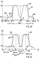
- the real intensity profile has been represented.
- the value of the intensities is shown inverted for ease of drawing. That is to say, a black object therefore having a luminance level weak, is represented by an intensity curve with positive values. Such a representation results from a pure convention without affecting the process of the invention.
- the algorithm described below is intended to determine the existence of one or more several branches, or objects when scanning by each line ⁇ ; O center (s) local (s) of the branch (es) on the line ⁇ considered; the half width (s) local (s) "a" of the branch (es) on the line ⁇ in question; that is to say by example the position "yo" of the center O of the segment I1 delimited by the section of the branch 1 by the scanning line A1, as well as the half-width "a” of this segment I1 on this line A1, leading to the determination of the position of the ends ⁇ and ⁇ of this segment I1 on the scanning line A1.
- This algorithm is capable of performing this determination whatever the respective width of these branches or objects, that is to say branches that are several tens of pixels wide, or only a few pixels; and regardless of the distance between the different branches or objects from each others, i.e. a distance of several tens of pixels or only a few pixels.
- M (y) a binary function forming an ideal model approaching as close as possible to the real profile g (y) as shown in FIG. 2A, 2B, 2C by way of example.
- This binary function would therefore be the function representing the ideal transverse intensity profile along the scanning line ⁇ , of a completely uniform object on a completely uniform background.
- This model is called " hat " below.
- M (y) be a cap chosen to correspond to the profile g (y) of FIG.2A.
- the hat M (y) has its center O in coincidence with that of section I1, therefore with that of profile g (y); further the cap M (y) has the ends of its central part in coincidence with the ends ⁇ , ⁇ of this section I1; therefore the half width of the object 1 measured by the half width of section I1 on the scanning line A1 of FIG.1A is equal to the value of the half width of the central part Ma of the hat.
- the model, or hat of FIG. 2A by means of 5 parameters: yo, Ga, Gb, a and b.
- y is the abscissa, measured in pixels, of the pixel current P on the sweep line ⁇ . If the scanning line ⁇ does not coincide with a row or column of pixels of the digital image, then you have to define on the right of ⁇ scanning of regularly spaced points whose intensity is determined by interpolation with respect to the intensity of the pixels considered in a given neighborhood. This method has been described above and is already known from the state of the art.
- the last pixel can be numbered 500, or 1000, depending on the size of the digital image and according to its definition. But, whether the line ⁇ is calibrated in pixels or in points, the numbers y1, y2, y3 ... yi ... yn of these pixels or points belong to the set N of positive integers.
- the current pixel Pi is fixed in the middle position yo of the hat on the line ⁇ , and it is considered that the quadratic error E is minimal when the hat M (y) is ideally centered at the point 0 middle of the object whose center and edges are sought, so when all the midpoints are at 0 and have the abscissa yo.
- the area covered by the central part Ma of the cap M (y) is defined by: y ⁇ Ma when y ⁇ [yo-a, yo + a]
- the area covered by one and the other outer portions of the hat, and Mb1 Mb2 is defined by: y ⁇ (Mb1, Mb 2) when: y ⁇ [yo- (a + b), yo- (a + 1)] U [yo + a + 1, yo + a + b] ⁇ N where N is the set of natural numbers.
- S t / 2 represents the difference between the cumulative sum of the squared intensities in the pixel interval between the first pixel of ⁇ and yo + a + b, and the cumulative sum of the squared intensities in the pixel interval between the first pixel of ⁇ and yo-a-b-1.
- this element S t / 2 represents the cumulative sum of the intensities of the pixels, squared, over any the length Lt of the hat centered in yo, which is considered to be the position of the pixel current Pi set in yo for this step of the calculation.
- S a / 1 represents the difference between the cumulative sum of the simple (i.e. non-square) intensities of the pixels located in the interval between the first pixel of ⁇ and yo + a, and the cumulative sum of the intensities single pixels in the interval between the first pixel of ⁇ and yo-a-1.
- S b 2/1 represents the difference between the cumulative sum of the simple intensities of the pixels located in the interval between the first pixel of ⁇ and yo + a + b, and the cumulative sum of the simple intensities in the interval between the first pixel of ⁇ and yo + a.
- S b1 / 1 represents the difference between the cumulative sum of the simple intensities of the pixels located in the interval between the first pixel of ⁇ and yo-a-1, and the cumulative sum of the intensities simple pixels located in the interval between the first pixel of ⁇ and yo-a-b-1.
- the scanning line A3 can cut a branch such as 5 whose general direction is parallel to this line of scanning.
- this first method has a defect in the event that it there are, in the digital image to be processed, branches or separate objects one of the other by a small number of pixels, a few pixels.
- the error E is minimized when the hat is positioned astride the two peaks intensity profiles that result from this situation when scanning the image; that is the case of a scan represented particularly by the line A2 of FIG.1A, the corresponding intensity profiles being shown in FIG.2B. So in the situation from FIG. 2B, the error is minimized when the hat frames the two intensity peaks, whereas if the hat is centered on one or the other of the two peaks, the error is very big.
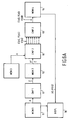
- FIG. 6C schematically represents the result obtained at the output of fourth MEM4 storage means, i.e. the abscissa on the line ⁇ , in the image, from the center of the object, and the two half-widths a (yo) on either side of the center, allowing to appreciate the segment I.
- the arrangement of FIG. 6A makes it possible to treat all the scanning lines you want to delimit the centers and edges of an OBJ object with precision.
Landscapes
- Engineering & Computer Science (AREA)
- Computer Vision & Pattern Recognition (AREA)
- Theoretical Computer Science (AREA)
- General Physics & Mathematics (AREA)
- Physics & Mathematics (AREA)
- Medical Informatics (AREA)
- Quality & Reliability (AREA)
- Radiology & Medical Imaging (AREA)
- Nuclear Medicine, Radiotherapy & Molecular Imaging (AREA)
- Health & Medical Sciences (AREA)
- General Health & Medical Sciences (AREA)
- Image Analysis (AREA)
- Image Processing (AREA)
Description
L'invention concerne un procédé de traitement d'une image, laquelle comporte la représentation d'au moins un objet constitué de pixels d'intensité sensiblement uniforme, contrastant sur un fond constitué de pixels d'intensité sensiblement uniforme. L'invention concerne également un arrangement pour mettre en oeuvre ce procédé.The invention relates to a method for processing an image, which includes the representation of at least one object made up of pixels of intensity substantially uniform, contrasting on a background consisting of pixels of intensity substantially uniform. The invention also relates to an arrangement for setting up this process.
L'invention trouve son application dans la détermination des contours de tout objet, représenté dans une image, qui montre un contraste vis-à-vis d'un fond sensiblement uniforme. L'invention trouve par exemple son application dans le domaine des systèmes de formation d'images numérisées, pour aider à la détection d'anomalies telles que des sténoses à partir d'angiographies du corps humain ou animal.The invention finds its application in determining the contours of any object, represented in an image, which shows a contrast against a background substantially uniform. The invention finds, for example, its application in the field digital imaging systems to assist in the detection of anomalies such as strictures from angiograms of the human or animal body.
Les angiographies sont des images spécialisées, pour la visualisation des vaisseaux sanguins. Plusieurs types d'angiographies sont réalisables : les angiographies coronariennes, pour la visualisation des artères irriguant le muscle du coeur, ou myocarde, l'ensemble de ces artères formant l'arbre coronarien ; les angiographies périphériques pour visualiser l'irrigation des membres inférieurs et supérieurs ; les angiographies cérébrales. On s'intéressera ci-après à titre d'exemple aux angiographies coronariennes. Les sténoses sont des rétrécissements locaux provoqués par des obstructions partielles ou totales qui apparaissent sur des artères. Dans le cas de l'arbre coronarien, les sténoses compromettent gravement l'irrigation du myocarde et doivent être détectées par un praticien à partir des angiographies.Angiographies are specialized images, for the visualization of blood vessels. Several types of angiographies are possible: angiographies coronary, for viewing the arteries supplying the heart muscle, or myocardium, all of these arteries forming the coronary tree; angiographies peripherals to visualize the irrigation of the lower and upper limbs; the cerebral angiographies. As an example, we will focus on angiography below. coronary. Stenoses are local narrowing caused by partial or total obstructions that appear on arteries. In the case of the tree coronary artery stenosis seriously compromises myocardial irrigation and must be detected by a practitioner from angiograms.
L'introduction, ces dernières années, de la radiographie numérisée, qui combine l'utilisation d'un détecteur de rayons X donnant une image en temps réel et la numérisation des images, a constitué un progrès majeur dans le domaine de la formation d'images, par rapport à la radiographie conventionnelle. Elle donne en effet accès aux nombreuses possibilités offertes par les techniques de traitement numérique d'images. D'autres méthodes de formation d'images angiographiques sont également connues, telles que les méthodes utilisant la résonance magnétique nucléaire. Dans tous les cas, l'invention ne tient pas compte de la méthode par laquelle l'image numérique a été obtenue, ni de la nature des objets qu'elle représente, mais concerne seulement le traitement de cette image numérique pour déterminer les points centraux et les points des bords des objets représentés, pourvu que ces objets constituent des masses suffisamment uniformes contrastant sur un fond suffisamment uniforme.The introduction in recent years of digital radiography, which combines the use of an X-ray detector giving a real-time image and the digitization of images, was a major advance in the field of training images, compared to conventional radiography. It gives access to many possibilities offered by digital image processing techniques. Other methods of forming angiographic images are also known, such as methods using nuclear magnetic resonance. In all cases, the invention does not take into account the method by which the digital image was obtained, or the nature of the objects it represents, but only concerns the processing of this digital image to determine the central points and the points edges of the objects represented, provided that these objects constitute masses sufficiently uniform contrasting on a sufficiently uniform background.
Un procédé d'identification automatisé des contours de vaisseaux dans
des angiographies coronariennes est connu de la publication intitulée "Automated
Identification of Vessel Contours in Coronary Arteriograms by an adaptive Tracking
Algorithm", par Ying SUN, dans IEEE Transactions on Medical Imaging, Vol.8, N°1, March
1989. Ce document décrit un algorithme de "suivi du tracé" dit "tracking" de la ligne
centrale des vaisseaux, pour l'identification des contours de ces vaisseaux dans des
angiographies numérisées. L'algorithme comprend essentiellement trois étapes qui sont :
Un premier problème technique qui se pose dans le traitement d'image des angiographies est la détection de toutes les situations pathologiques, et l'élimination des fausses alarmes. Les situations pathologiques, contrairement à ce qui est indiqué dans le document cité, ne comprennent pas uniquement les sténoses qui apparaissent sous la forme d'un rétrécissement local dans un vaisseau, lequel montre donc simplement un minimum local de largeur. Les situations pathologiques comprennent aussi un type de rétrécissement dit "en marche d'escalier" qui apparaít sur un vaisseau d'une première largeur sensiblement uniforme, par le passage abrupt à une seconde largeur inférieure à la première. Ce genre de "marche d'escalier" peut signifier que l'on a affaire à un vaisseau dit principal, d'une première largeur, qui se divisait en deux vaisseaux dont l'un, de la seconde largeur, est toujours visible dans le prolongement du vaisseau principal, mais dont l'autre est maintenant complètement occlus à partir de son embranchement avec le vaisseau principal et a désormais disparu, étant devenu complètement invisible sur l'angiographie. L'unique moyen de détecter ce vaisseau complètement occlus et désormais invisible, est de détecter le rétrécissement en "marche d'escalier" sur le vaisseau principal.A first technical problem that arises in image processing angiography is the detection of all pathological situations, and the elimination false alarms. Pathological situations, contrary to what is indicated in the cited document, do not include only the strictures that appear in the form of a local narrowing in a vessel, which therefore simply shows a local minimum of width. Pathological situations also include a type of narrowing said "staircase" that appears on a vessel of a first substantially uniform width, by steep transition to a second width less than the first one. This kind of "stair step" can mean that we are dealing with a so-called main vessel, of a first width, which was divided into two vessels, one of which, of the second width, is always visible in the extension of the main vessel, but the other of which is now completely occluded from its junction with the main ship and has now disappeared, having become completely invisible on angiography. The only way to detect this completely occluded vessel and now invisible, is to detect the narrowing in "stair step" on the main vessel.
Cette dernière situation pathologique ne peut pas être reconnue par l'algorithme décrit dans l'état de la technique cité ; ceci parce que le "suivi du tracé" ou "tracking" du vaisseau est prévu pour suivre le tracé du vaisseau principal et éliminer celui de vaisseaux secondaires. Ainsi, le procédé connu est incapable de distinguer le cas où il apparaít une "marche d'escalier" dû au fait qu'à l'embranchement l'un des deux vaisseaux secondaires a complètement disparu qui est un cas pathologique grave, du cas non pathologique où les deux vaisseaux secondaires sont toujours présents à l'embranchement. Comme la forme caractéristique en "marche d'escalier" est l'unique alarme permettant au praticien de déceler les vaisseaux occlus, ce type d'algorithme n'offre pas au praticien la possibilité de détecter ces situations pathologiques qui sont à la fois importantes en nombre et en gravité regardant l'état du patient.This latter pathological situation cannot be recognized by the algorithm described in the cited state of the art; this is because "tracking" or "tracking" of the ship is planned to follow the course of the main ship and eliminate that of secondary vessels. Thus, the known method is unable to distinguish the case where there appears a "stair step" due to the fact that at the fork one of the two secondary vessels has completely disappeared which is a serious pathological case of the case non-pathological where the two secondary vessels are always present at the fork. As the characteristic shape in "stair step" is the unique alarm allowing the practitioner to detect occluded vessels, this type of algorithm does not offer the practitioner the possibility of detecting these pathological situations which are at the times important in number and severity looking at the patient's condition.
Un second problème technique qui se pose est la réalisation d'appareils de radiologie munis de moyens pour la détection totalement automatique des situations pathologiques décrites plus haut, à savoir la première situation de rétrécissement local de vaisseaux, et la seconde situation de rétrécissement en "marche d'escalier". Par détection totalement automatique, on entend que la mise en évidence des situations pathologiques doit être réalisée sans l'aide d'un opérateur.A second technical problem which arises is the production of apparatus radiology equipped with means for fully automatic detection of situations pathologies described above, namely the first situation of local shrinkage of vessels, and the second situation of narrowing in "staircase steps". By detection fully automatic, we mean that the highlighting of pathological situations must be performed without the help of an operator.
La réalisation d'angiographies suppose qu'un patient, en général éveillé, se voit injecter, par exemple par l'artère fémorale au moyen d'un cathéter, un produit contrastant ; puis un opérateur réalise une série de radiographies de l'arbre coronarien sous la forme d'une séquence d'images vidéo à raison de 30 images par seconde, par exemple. Une telle séquence permet ainsi de visualiser plusieurs cycles cardiaques. Les sténoses ou rétrécissements décrits plus haut sont les principales anormalités à détecter. Mais cette détection peut être rendue difficile en raison d'une orientation peu favorable des vaisseaux, ou du passage d'un vaisseau à l'arrière plan derrière un vaisseau situé en premier plan. Il est donc nécessaire d'exploiter différents angles de projection et aussi de tenter de détecter les sténoses dans toutes les images de la séquence vidéo pour lesquelles la concentration du produit contrastant est suffisamment forte pour assurer une bonne visibilité des vaisseaux.Performing angiograms assumes that a patient, usually awake, is injected, for example by the femoral artery by means of a catheter, a product contrasting; then an operator performs a series of x-rays of the coronary tree as a sequence of video images at a rate of 30 frames per second, per example. Such a sequence thus makes it possible to visualize several cardiac cycles. The strictures or strictures described above are the main abnormalities to be detected. But this detection can be made difficult due to an unfavorable orientation vessels, or the passage of a vessel in the background behind a vessel located in foreground. It is therefore necessary to use different projection angles and also to attempt to detect strictures in all images in the video sequence to which the concentration of the contrasting product is high enough to ensure good visibility of the vessels.
Les clichés sont donc assez nombreux, et le praticien établit son diagnostic en faisant défiler ces images lentement devant ses yeux. Il apparaít alors un besoin pour mettre en évidence à l'avance et de manière automatique les situations pathologiques dont on a parlé plus haut. En effet, le praticien a tendance, psychologiquement, à voir son attention attirée par les situations pathologiques les plus flagrantes, et à laisser passer certaines situations moins visibles, mais qui peuvent être plus gênantes, ou plus graves, cliniquement, pour l'avenir du patient. Ou bien le praticien peut laisser passer certaines situations pathologiques parce qu'elles n'apparaissent que dans une seule image, ou dans peu d'images de la séquence.The pictures are therefore quite numerous, and the practitioner establishes his diagnosis by scrolling these images slowly before his eyes. It then appears need to automatically highlight situations in advance pathological of which we spoke above. Indeed, the practitioner tends, psychologically, to see his attention drawn to the most pathological situations flagrant, and to let pass certain less visible situations, but which can be more embarrassing, or more serious, clinically, for the patient's future. Or the practitioner can let pass certain pathological situations because they appear only in a single image, or in few images in the sequence.
Il est donc important que le praticien puisse disposer d'un système de mise en évidence des situations pathologiques de manière à attirer son attention sur les endroits des images, ou les endroits de l'unique ou des quelques images de la séquence qui contiennent en fait les informations les plus intéressantes, qu'il est indispensable d'examiner. Son attention pourra ainsi être attirée sur les endroits les moins vraisemblables a priori, mais qui contiennent néanmoins des situations pathologiques ; et par ailleurs, son attention pourra être détournée de se focaliser sur quelques sténoses évidentes mais sans grande importance sur le plan des suites médicales. It is therefore important that the practitioner has a system of highlighting pathological situations so as to draw attention to the locations of the images, or the locations of the single or a few images of the sequence which contain in fact the most interesting information, which is essential to examine. His attention can thus be drawn to the least probable a priori, but which nevertheless contain pathological situations; and moreover, his attention may be diverted from focusing on a few strictures obvious but unimportant in terms of medical outcomes.
Une telle automatisation totale de la détection des situations pathologiques ne peut être mise en oeuvre que si l'on réussit préalablement à rendre automatique la détection de la position des objets dans l'image numérique, par exemple par la détermination de la position de leurs points de centres, et si l'on réussit en outre, préalablement, à rendre automatique la détection de la position de leurs bords, ou de leurs contours, par exemple par la détermination de leur demi largeur dans une direction donnée, à partir du point de centre correspondant.Such total automation of situation detection pathological can only be implemented if we previously succeed in rendering automatic detection of the position of objects in the digital image, for example by determining the position of their center points, and if we also succeed, beforehand, to make automatic the detection of the position of their edges, or their contours, for example by determining their half width in a direction given, from the corresponding center point.
Une telle automatisation de la détermination des lignes de centres et des lignes de contours conduit à pouvoir ultérieurement rendre automatique la détection de toute anomalie portant sur les dimensions ou la forme des objets dans l'image numérique.Such automation of the determination of center lines and contour lines means that the detection of any anomaly relating to the dimensions or shape of the objects in the image digital.
Une telle automatisation totale de la détection des situations pathologiques ne peut être obtenue si l'on utilise l'algorithme connu du document cité.Such total automation of situation detection pathological cannot be obtained using the algorithm known from the cited document.
Cet algorithme connu du document cité n'est pas assez robuste pour permettre une automatisation ultérieure totale du procédé de détection de sténoses. Le manque de robustesse est dû au fait que l'algorithme détermine les points de la ligne de centre de vaisseau par des approximations successives à partir d'un point de départ, et parce qu'il utilise des profils de densité d'images bruitées. Des erreurs peuvent ainsi s'accumuler, ce qui est un inconvénient lorsqu'un automatisme poussé est envisagé. De ce fait, ou bien cet algorithme peut conduire à suivre des chemins qui ne sont pas des vaisseaux : il peut s'égarer. Ou bien il conduit à laisser de côté des chemins intéressants. Il faut alors le remettre sur le chemin que l'on veut réellement suivre. Il en résulte que, dû à ce manque de robustesse, il a besoin d'être guidé.This algorithm known from the cited document is not robust enough to allow total subsequent automation of the stenosis detection process. The lack of robustness is due to the fact that the algorithm determines the points of the line of center of the vessel by successive approximations from a starting point, and because it uses noisy image density profiles. Errors can thus accumulate, which is a drawback when a high degree of automation is envisaged. Of this fact, or else this algorithm can lead to following paths which are not vessels: it can go astray. Or it leads to leaving out interesting paths. It must then be put back on the path that we really want to follow. It follows that, due to this lack of robustness, it needs to be guided.
D'autre part, dans le cas où une bifurcation apparaít lors du suivi du tracé d'un vaisseau, l'algorithme connu est prévu pour suivre la branche qui montre l'intensité la plus grande, éliminant ainsi le suivi du tracé du vaisseau secondaire, car cet algorithme connu ne peut se permettre de traiter le problème qui apparaít lorsque le profil d'intensité montre un double pic. L'examen des vaisseaux secondaires doit donc se faire en repositionnant le "point de départ" de l'algorithme à l'endroit de l'embranchement, sur le vaisseau secondaire abandonné lors d'un premier passage, pour effectuer maintenant les étapes de l'algorithme en suivant ce vaisseau secondaire. Pour suivre l'ensemble des vaisseaux d'une région vitale considérée, l'algorithme connu a donc, pour cette raison supplémentaire, encore besoin d'être guidé, et n'est donc pas automatisable. On the other hand, in the case where a bifurcation appears during the monitoring of layout of a vessel, the known algorithm is planned to follow the branch which shows the greatest intensity, eliminating tracking of the secondary vessel because this known algorithm cannot afford to deal with the problem that arises when the intensity profile shows a double peak. The examination of the secondary vessels must therefore be do this by repositioning the "starting point" of the algorithm at the location of the branch line, on the secondary vessel abandoned during a first pass, to Now perform the steps of the algorithm by following this secondary vessel. For follow all the vessels of a vital region considered, the known algorithm therefore has, for this additional reason, still needs to be guided, and therefore is not automatable.
On notera que, en référence avec la FIG.2 du document cité, un profil d'intensité idéal, de forme rectangulaire, est utilisé pour réaliser une convolution avec le profil d'intensité obtenu par balayage transversal du vaisseau étudié, afin de déterminer un vecteur dont on cherche la valeur maximale, laquelle est relative au pixel correspondant au maximum du profil d'intensité mesuré. Ce pixel est retenu comme point de la ligne de centre mis à jour. Pour effectuer cette opération, la largeur du profil idéal rectangulaire est fixée A PRIORI. La largeur réelle du vaisseau n'est pas déterminable lors de cette étape de l'algorithme.It will be noted that, with reference to FIG. 2 of the cited document, a profile of ideal intensity, rectangular in shape, is used to achieve convolution with the intensity profile obtained by transverse scanning of the vessel studied, in order to determine a vector whose maximum value is sought, which is relative to the pixel corresponding to the maximum of the intensity profile measured. This pixel is retained as point of the updated center row. To perform this operation, the ideal profile width rectangular is fixed A PRIORI. The actual width of the vessel is not determinable when of this step of the algorithm.
La détermination de la largeur des vaisseaux est réalisée dans une étape ultérieure, en identifiant les bords du vaisseau comme les points d'inflexion de part et d'autre du maximum du profil d'intensité transversal mesuré du vaisseau. Cette étape donne une mise à jour de la largeur locale du vaisseau qui sera utilisée pour déterminer la largeur du profil idéal rectangulaire utilisé dans la détermination du point de centre suivant lors d'une étape ultérieure.The determination of the width of the vessels is carried out in one step subsequent, identifying the edges of the vessel as the inflection points on the part and on the other side of the maximum of the transverse intensity profile measured of the vessel. This step gives an update of the local width of the ship which will be used to determine the width of the ideal rectangular profile used in determining the center point next in a later step.
La présente invention a pour but de fournir un procédé pour déterminer, dans une image comportant la représentation d'objets sensiblement uniformes contrastant sur un fond sensiblement uniforme, les points centraux ainsi que les demi largeurs locales de sections des objets par des droites de balayage de directions prédéterminées.The object of the present invention is to provide a method for determining, in an image comprising the representation of substantially uniform objects contrasting on a substantially uniform background, the central points as well as the half local section widths of objects by direction scanning lines predetermined.
La présente invention a particulièrement pour but de déterminer ainsi les points de centre et les points des bords d'objets qui ne sont pas nécessairement les branches de vaisseaux sanguins mais qui peuvent être tout autre objet d'une image répondant aux conditions de contraste.The present invention particularly aims to thus determine the center points and the points of the edges of objects which are not necessarily the branches of blood vessels but which can be any other object of an image meeting the contrast conditions.
La présente invention a particulièrement pour but de fournir un tel procédé qui soit robuste, c'est-à-dire dont la détermination d'un point ne dépende pas de la détermination d'un point précédent suivie d'une approximation.The present invention particularly aims to provide such a process which is robust, that is to say the determination of a point does not depend on the determination of a previous point followed by an approximation.
La présente invention a aussi pour but de fournir un tel procédé qui n'ait pas besoin d'être guidé, c'est-à-dire à qui l'on n'est pas besoin d'imposer des points de départ, ou à qui l'on n'a pas besoin d'imposer une zone de recherche particulière.The present invention also aims to provide such a process which does not have no need to be guided, that is to say one who does not need to impose points of departure, or on which one does not need to impose a particular search area.
La présente invention a aussi pour but de fournir un procédé capable de travailler à toute résolution, et qui permette la détermination de la largeur d'un objet quelle que soit la largeur déterminée lors d'une étape antérieure.The present invention also aims to provide a method capable of work at any resolution, and which allows the determination of the width of an object whatever the width determined in an earlier step.
La présente invention a encore pour but de fournir un tel procédé qui ne laisse pas de côté des objets de trop petites ou trop grandes dimensions ou des objets disposés les uns des autres à des très faibles distances et qui soit capable de mettre en évidence des discontinuités dans cette structure.Another object of the present invention is to provide such a method which does not do not leave too small or too large objects or objects arranged at very short distances from each other and capable of evidence of discontinuities in this structure.
La présente invention a particulièrement pour but de fournir une telle méthode qui soit complètement automatisable.The present invention particularly aims to provide such a method which is completely automatable.
Ces buts sont atteints au moyen d'un procédé selon la Revendication 1.These objects are achieved by a method according to Claim 1.
Une mise en oeuvre de ce procédé, pour la construction de ladite seconde fonction des sommes cumulées, est caractérisé par les éléments de la Revendication 2.An implementation of this process, for the construction of said second function of the accumulated sums, is characterized by the elements of the Claim 2.
Ainsi le procédé selon l'invention est robuste. Les points et valeurs déterminés le sont d'une manière absolue, non par une approximation à partir d'une valeur ou d'un point précédent. Ceci est très différent de la méthode connue et constitue un avantage essentiel en vue de rendre le procédé automatique.Thus the method according to the invention is robust. Points and values determined in an absolute way, not by an approximation from a value or a previous point. This is very different from the known method and constitutes an essential advantage in order to make the process automatic.
En outre, le procédé selon l'invention, n'a pas besoin d'être guidé, mais détermine systématiquement tous les points de bord d'un objet dès que cet objet est rencontré par une droite de balayage. Il est donc essentiellement automatisable. Il ne laisse aucun objet de côté, que ce soit pour des raisons de forme ou des raisons de dimension comme le faisait la méthode connue. Ceci est aussi une grande différence et un avantage essentiel vis-à-vis de la méthode connue.Furthermore, the method according to the invention does not need to be guided, but systematically determines all the edge points of an object as soon as this object is encountered by a sweep line. It is therefore essentially automatable. He ... not leaves no object behind, whether for reasons of form or reasons of dimension as the known method did. This is also a big difference and an essential advantage over the known method.
De plus, le procédé selon l'invention permet de distinguer les bords de deux objets même très rapprochés, alors que la méthode connue, ou bien confondait les objets, ou bien laissait l'un d'eux de côté. Le procédé selon l'invention est donc très précis. Ceci est une grande différence et un autre avantage essentiel de l'invention.In addition, the method according to the invention makes it possible to distinguish the edges of two objects even very close together, while the known method, or else confused the objects, or left one of them aside. The process according to the invention is therefore very specific. This is a big difference and another essential advantage of the invention.
Dans une mise en oeuvre particulière, ce procédé de traitement d'image est caractérisé par les éléments de la Revendication 3.In a particular implementation, this image processing method is characterized by the elements of Claim 3.
Dans une mise en oeuvre préférentielle, ce procédé est caractérisé en ce qu'il comprend les éléments de la Revendication 4.In a preferred implementation, this process is characterized in that that it includes the elements of Claim 4.
Donc, selon l'invention, les points de centre et les demi-largeurs sont déterminés par un même processus qui inclut uniquement le calcul de sommes cumulées d'intensités de pixel, ou d'intensités au carré, sur une droite de balayage. Ces calculs sont rapides et faciles à mettre en oeuvre. Le procédé selon l'invention est donc là encore particulièrement avantageux. Chaque détermination de centre et de demi-largeur associée est effectuée pour une droite de balayage donnée, indépendamment de toute autre détermination antérieure ou ultérieure. Donc en prévoyant un nombre de droites de balayage adéquat, on obtient selon l'invention une détermination robuste et précise des points des lignes de centres et de bords. La prédétermination des directions des droites de balayage ne dépend de rien d'autre que du souci de couvrir correctement l'image pour déterminer un nombre de points suffisant. Ces directions peuvent être avantageusement les directions de balayage parallèles par lignes et colonnes connues de l'homme du métier. Mais toute autre direction de balayage est aussi possible.Therefore, according to the invention, the center points and the half-widths are determined by the same process which includes only the calculation of accumulated sums pixel intensities, or squared intensities, on a scan line. These calculations are quick and easy to set up. The process according to the invention is therefore there again particularly advantageous. Each center and half-width determination associated is performed for a given sweep line, independently of any other prior or subsequent determination. So by providing a number of lines of adequate scanning, a robust and precise determination of the points of the center and edge lines. The predetermination of the directions of the lines depends on nothing more than the concern to cover the image correctly for determine a sufficient number of points. These directions can advantageously be the parallel scanning directions by lines and columns known to those skilled in the art job. But any other scanning direction is also possible.
L'invention propose en outre un arrangement pour procéder au traitement d'une image, laquelle comporte la représentation d'au moins un objet OBJ constitué de pixels d'intensité sensiblement uniforme, contrastant sur un fond constitué de pixels d'intensité sensiblement uniforme, cet arrangement comprenant les éléments de la Revendication 12.The invention further provides an arrangement for carrying out image processing, which includes the representation of at least one OBJ object consisting of pixels of substantially uniform intensity, contrasting on a background formed pixels of substantially uniform intensity, this arrangement comprising the elements of Claim 12.
En particulier, l'invention propose un arrangement tel que le précédent, comprenant en outre les éléments de la Revendication 13.In particular, the invention proposes an arrangement such as the previous one, further comprising the elements of Claim 13.
L'invention est décrite ci-après en détail en référence avec les figures
schématiques annexées dont :
Dans un exemple décrit à titre non limitatif, la présente invention concerne une méthode pour déterminer, dans une image, numérique ou non numérique, telle que montrée sur la FIG.1A représentant une structure arborescente, la largeur de chaque branche de la structure par la détermination des points situés au centre de ces branches et des points localisés sur les bords de ces branches. La présente méthode peut être appliquée sans modification de ses moyens à la détermination de la position des points de centre et des points des bords de tout objet contrastant sur un fond uniforme dans une image numérique ou non numérique. D'une manière générale, la présente invention concerne un procédé de traitement d'une image, laquelle comporte la représentation d'au moins un objet constitué de pixels d'intensité sensiblement uniforme contrastant sur un fond constitué de pixels d'intensité sensiblement uniforme. Par "intensité sensiblement uniforme contrastant sur", on entend que les variations d'intensité sur la surface de l'objet sont d'un ordre de grandeur, c'est-à-dire environ 10 fois, ou au moins 10 fois, plus petites que la différence entre l'intensité moyenne des pixels de l'objet et l'intensité moyenne des pixels du fond environnant. In an example described without limitation, the present invention relates to a method for determining, in an image, digital or non-digital, as shown in FIG. 1A representing a tree structure, the width of each branch of the structure by determining the points located at the center of these branches and points located on the edges of these branches. This method can be applied without modification of its means to the determination of the position of center points and edge points of any contrasting object on a uniform background in a digital or non-digital image. In general, this The invention relates to a method for processing an image, which comprises representation of at least one object consisting of pixels of substantially uniform intensity contrasting on a background consisting of pixels of substantially uniform intensity. Through "substantially uniform intensity contrasting on" means that variations in intensity on the surface of the object are of an order of magnitude, i.e. about 10 times, or at least minus 10 times, smaller than the difference between the average pixel intensity of the object and the average intensity of the pixels of the surrounding background.
Une des particularités de l'invention est qu'elle concerne une méthode, ou algorithme, applicable au moyen d'un balayage systématique et automatique de l'image par des droites de directions prédéterminées. L'algorithme est mis en oeuvre par balayage selon cette série de droites parallèles à une direction donnée. Puis, éventuellement, par exemple dans le cas d'une image numérique, l'algorithme peut être mis en oeuvre par balayage selon une seconde, voire une troisième, etc.. séries de droites parallèles à une deuxième puis troisième direction donnée respectivement, de manière à mieux déterminer la largeur de toutes les branches de la structure ou de tous les objets pouvant avoir des orientations différentes dans le plan de l'image numérique.One of the features of the invention is that it relates to a method, or algorithm, applicable by means of a systematic and automatic scanning of the image by lines of predetermined directions. The algorithm is implemented by scanning along this series of lines parallel to a given direction. Then, possibly, for example in the case of a digital image, the algorithm can be implemented by scanning according to a second or even a third, etc. series of lines parallel to a second then third direction given respectively, so that better determine the width of all the branches of the structure or of all the objects may have different orientations in the digital image plane.
Dans une mise en oeuvre simple appliquée à une image numérique, le balayage peut être effectué selon les lignes et/ou les colonnes de pixels de l'image numérique, mais non pas exclusivement. Toutes les directions de balayage sont possibles ; y compris des directions ne passant pas exclusivement par des pixels. Dans le cas d'une image numérique, il faut noter que les directions de balayage et le nombre de droites de balayage dans chaque direction est choisi complètement A PRIORI par l'homme du métier, avec comme seuls but et condition, la précision recherchée, c'est-à-dire la distance entre chaque ligne de balayage qui définit finalement le nombre de mesures fournies par le procédé.In a simple implementation applied to a digital image, the scanning can be performed according to the rows and / or columns of pixels in the image digital, but not exclusively. All scanning directions are possible ; including directions not passing exclusively through pixels. In the case of a digital image, it should be noted that the scanning directions and the number of lines of scanning in each direction is chosen completely PRIORI by the man of the profession, with only aim and condition, the desired precision, that is to say the distance between each scan line which ultimately defines the number of measurements provided by the process.
En référence à la FIG.1A, on supposera dans ce qui suit que l'objet représenté, en l'occurrence ici, la structure arborescente à étudier, est d'intensité sensiblement uniforme, par exemple noire, sur un fond également sensiblement uniforme, par exemple blanc. Néanmoins, cette image présente plusieurs niveaux de luminance, et il en résulte que le profil d'intensité transversal d'une branche de la structure à étudier déterminé lors du balayage, n'est pas idéalement rectangulaire. Si le fond de l'image n'est pas suffisamment uniforme, l'homme du métier peut avoir recours à une étape préliminaire d'extraction du fond, telle que décrite à titre d'exemple non limitatif dans la demande de brevet européen N° EP-A-0 635 806. C'est pourquoi, dans la présente description, il n'est pas limitatif de parler de fond uniforme.With reference to FIG. 1A, it will be assumed below that the object represented, in this case here, the tree structure to be studied, is of intensity substantially uniform, for example black, on a background also substantially uniform, for example white. However, this image has several levels of luminance, and it follows that the transverse intensity profile of a branch of the structure to be studied determined during scanning, is not ideally rectangular. If the background of the image is not sufficiently uniform, the skilled person may have recourse to a preliminary stage of extraction of the bottom, as described by way of example not limiting in European patent application No. EP-A-0 635 806. This is why, in the present description, it is not limiting to speak of a uniform background.
En référence à la FIG.1A, on a représenté une image numérique 10, comportant à titre d'objets : en 1 une première branche de la structure arborescente, par exemple représentant un vaisseau sanguin ; en 2 et 3 respectivement des deuxième et troisième branches issues de l'embranchement 4. Les lignes, respectivement A1, A2, A3,..., B1 etc.. représentent des droites de balayage parallèles dans une première direction A et dans une seconde direction B. Chacune des droites de balayage coupe les objets selon des segments I1, I2... etc. Par exemple la droite de balayage A1 coupe la branche 1 selon le segment I1 ; la droite de balayage A2 coupe les branches 2 et 5 selon les segments I2 et I3 ; la droite de balayage A3 coupe la branche 2 selon le segment I6 ; la droite de balayage B1 coupe la branche 5 selon le segment I5.With reference to FIG. 1A, a digital image 10 has been represented, comprising as objects: in 1 a first branch of the tree structure, by example representing a blood vessel; in 2 and 3 respectively of the second and third branches from branch 4. Lines, respectively A1, A2, A3, ..., B1 etc. represent parallel scanning lines in a first direction A and in a second direction B. Each of the scanning lines intersects the objects according to segments I1, I2 ... etc. For example, the scanning line A1 cuts the branch 1 according to segment I1; scan line A2 cuts branches 2 and 5 according to segments I2 and I3; the scanning line A3 intersects the branch 2 along the segment I6; the scanning line B1 cuts the branch 5 along the segment I5.
L'image 10 est numérique, c'est-à-dire formée de pixels dotés chacun d'un niveau de luminance ou d'intensité. Le niveau de luminance ou d'intensité peut être repéré par exemple sur une échelle de niveaux de luminance graduée de 1 à 256. Les pixels les plus lumineux ou clairs sont affectés des niveaux de luminance les plus grands, et les pixels les moins lumineux, ou pixel sombres, sont affectés des niveaux de luminance les plus petits sur cette échelle. Selon l'invention, on fournit un procédé de traitement de l'image numérique 10, applicable aussi à une image non numérique, pour déterminer les positions des points centraux O ainsi que les positions des points extrêmes α, β des segments I1, I2,... déterminés par la section des objets de l'image par des droites A1, A2, A3,... B1... parallèles aux directions données, dites ci-après d'une manière générale, direction Δ. A cet effet, on cherche à calculer les demi largeurs des segments I1, I2..., ce qui permettra de déterminer les positions α, β, des extrémités de ces segments, une fois connues les positions des points centraux de ces segments, sur chacune des droites de balayage.Image 10 is digital, i.e. made up of pixels each with a level of luminance or intensity. The luminance or intensity level can be identified for example on a scale of luminance levels graduated from 1 to 256. The the brightest or clearest pixels are assigned the highest luminance levels, and the less bright pixels, or dark pixels, are affected by the levels of smallest luminance on this scale. According to the invention, a method of providing digital image processing 10, also applicable to a non-digital image, for determine the positions of the central points O as well as the positions of the extreme points α, β of the segments I1, I2, ... determined by the section of the objects of the image by lines A1, A2, A3, ... B1 ... parallel to the directions given, say below in a way general, direction Δ. To this end, we seek to calculate the half widths of the segments I1, I2 ..., which will determine the positions α, β, of the ends of these segments, once known the positions of the central points of these segments, on each of the scanning lines.
En référence à la FIG.1B, on cherche donc à déterminer, à partir de la
structure de la FIG.1A, les lignes de centre telles que :
En référence à la FIG.1C, on cherche aussi à déterminer les lignes de
bords des branches, telles que :
Lorsque ci-après on fera référence à un point calculé, au lieu d'un pixel, cela signifie qu'à ce point est associé un niveau de luminance déterminé par interpolation en fonction des niveaux de luminance des pixels choisis dans un voisinage autour de ce point ; par exemple un voisinage formé des 4 pixels les plus proches de ce point. On pourra également calculer la luminance d'un point, en choisissant un voisinage formé de pixels à diverses distances de ce point, en affectant la luminance de chacun de ces pixels d'un poids d'autant plus faible que ce pixel est éloigné du point considéré, et en affectant le point considéré d'une luminance obtenue en prenant en compte des luminances pondérées des pixels du voisinage.When below we will refer to a calculated point, instead of a pixel, this means that a luminance level determined by interpolation is associated with this point as a function of the luminance levels of the pixels chosen in a neighborhood around this period; for example a neighborhood formed by the 4 pixels closest to this point. We will also be able to calculate the luminance of a point, by choosing a neighborhood formed by pixels at various distances from this point, affecting the luminance of each of these pixels of a weight all the more weaker than this pixel is far from the point considered, and by affecting the point considered of a luminance obtained by taking into account luminances weighted neighborhood pixels.
Sur une droite de balayage Δ donnée on trouvera donc soit des pixels, soit des points, régulièrement répartis et dotés chacun d'un niveau de luminance. La position de chaque pixel ou point sera repérée sur la droite de balayage ▵ par son abscisse "y" mesurée en nombre de pixels dans le sens du balayage à partir du pixel origine de la droite de balayage. Un point ou pixel courant Pi donné sur la droite ▵ aura pour abscisse particulière "yi".On a given scanning line Δ we therefore find either pixels, or points, regularly distributed and each with a luminance level. The position of each pixel or point will be identified on the scanning line ▵ by its abscissa "y" measured in number of pixels in the direction of scanning from the pixel origin of the scan line. A current point or pixel Pi given on the right ▵ will have for particular abscissa "yi".
En référence à la FIG.2A, on a représenté le profil d'intensité réel transversal g(y) obtenu par balayage de l'image selon la droite A1 ; en référence aux FIG.2B et 2C, le profil d'intensité réel transversal g(y) obtenu par balayage de l'image selon la droite A2. Sur ces courbes, la valeur des intensités est représentée inversée pour la facilité du dessin. C'est-à-dire qu'un objet noir ayant donc un niveau de luminance faible, est représenté par une courbe d'intensité à valeurs positives. Une telle représentation résulte d'une pure convention sans incidence sur le procédé de l'invention.With reference to FIG. 2A, the real intensity profile has been represented. transverse g (y) obtained by scanning the image along the line A1; with reference to FIG. 2B and 2C, the real transverse intensity profile g (y) obtained by scanning the image along the line A2. On these curves, the value of the intensities is shown inverted for ease of drawing. That is to say, a black object therefore having a luminance level weak, is represented by an intensity curve with positive values. Such a representation results from a pure convention without affecting the process of the invention.
L'algorithme décrit ci-après est destiné à déterminer l'existence d'une ou plusieurs branches, ou objets lors du balayage par chaque droite ▵ ; le(s) centre(s) O local(aux) de la ou des branche(s) sur la droite Δ considérée ; la (les) demi- largeur(s) locales(s) "a" de la ou des branche(s) sur la droite Δ en question ; c'est-à-dire par exemple la position "yo" du centre O du segment I1 délimité par la section de la branche 1 par la droite de balayage A1, ainsi que la demi largeur "a" de ce segment I1 sur cette droite A1, conduisant à la détermination de la position des extrémités α et β de ce segment I1 sur la droite de balayage A1. Cet algorithme est capable d'effectuer cette détermination quelle que soit la largeur respective de ces branches ou objets, c'est-à-dire branches larges de plusieurs dizaines de pixels, ou de seulement quelques pixels ; et quelle que soit la distance qui sépare les différentes branches ou objets les uns des autres, c'est-à-dire distance de plusieurs dizaines de pixels ou de seulement quelques pixels.The algorithm described below is intended to determine the existence of one or more several branches, or objects when scanning by each line ▵; O center (s) local (s) of the branch (es) on the line Δ considered; the half width (s) local (s) "a" of the branch (es) on the line Δ in question; that is to say by example the position "yo" of the center O of the segment I1 delimited by the section of the branch 1 by the scanning line A1, as well as the half-width "a" of this segment I1 on this line A1, leading to the determination of the position of the ends α and β of this segment I1 on the scanning line A1. This algorithm is capable of performing this determination whatever the respective width of these branches or objects, that is to say branches that are several tens of pixels wide, or only a few pixels; and regardless of the distance between the different branches or objects from each others, i.e. a distance of several tens of pixels or only a few pixels.
Selon l'une et l'autre des méthodes décrites ci-après, on cherche d'abord à déterminer un modèle binaire capable de coller au mieux au profil d'intensité réel transversal g(y) obtenu par le balayage selon une droite Δ choisie parmi toutes les droites de balayage Δ possibles de l'image numérique. According to either of the methods described below, we first seek to determine a binary model capable of sticking best to the real intensity profile transverse g (y) obtained by scanning along a line Δ chosen from all the lines possible scanning Δ of the digital image.
On cherche d'abord une fonction binaire M(y) formant un modèle idéal s'approchant au plus près du profil réel g(y) tel que représenté sur les FIG.2A, 2B, 2C à titre d'exemple. Cette fonction binaire serait donc la fonction représentant le profil d'intensité transversal idéal selon la droite de balayage Δ, d'un objet totalement uniforme sur un fond totalement uniforme. On appelle ci-après "chapeau" ce modèle. Soit M(y) un chapeau choisi pour correspondre au profil g(y) de la FIG.2A.We first look for a binary function M (y) forming an ideal model approaching as close as possible to the real profile g (y) as shown in FIG. 2A, 2B, 2C by way of example. This binary function would therefore be the function representing the ideal transverse intensity profile along the scanning line Δ, of a completely uniform object on a completely uniform background. This model is called " hat " below. Let M (y) be a cap chosen to correspond to the profile g (y) of FIG.2A.
Tel que représenté sur la FIG.2A, soit "yo" l'abscisse du milieu O de ce
chapeau M(y) le long de la droite Δ et Lt sa largeur totale. Le chapeau a une largeur
centrale
La = (2a+1) pixels, et deux bords de largeur Lb1 = Lb2 = b pixels chacun. La hauteur du
chapeau au centre, c'est-à-dire l'intensité des pixels dans la partie centrale Ma du
chapeau, est notée Ga, et la hauteur du chapeau de part et d'autre de la partie centrale,
c'est-à-dire l'intensité des pixels dans ces parties dites externes Mb1 et Mb2, est notée
Gb.As shown in FIG.2A, let "yo" be the abscissa of the middle O of this cap M (y) along the line Δ and Lt its total width. Hat has central width
La = (2a + 1) pixels, and two edges of width Lb1 = Lb2 = b pixels each. The height of the hat in the center, that is to say the intensity of the pixels in the central part Ma of the hat, is denoted Ga, and the height of the hat on either side of the central part is ie the intensity of the pixels in these so-called external parts Mb1 and Mb2, is noted Gb.
Dans la représentation idéale de la FIG.2A, le chapeau M(y) a son centre O en coïncidence avec celui de la section I1, donc avec celui du profil g(y) ; en outre le chapeau M(y) a les extrémités de sa partie centrale en coïncidence avec les extrémités α, β de cette section I1 ; par conséquent la demi largeur de l'objet 1 mesurée par la demi largeur de la section I1 sur la droite de balayage A1 de la FIG.1A est égale à la valeur de la demi largeur de la partie centrale Ma du chapeau. On a donc défini le modèle, ou chapeau de la FIG.2A, au moyen de 5 paramètres : yo, Ga, Gb, a et b.In the ideal representation of FIG. 2A, the hat M (y) has its center O in coincidence with that of section I1, therefore with that of profile g (y); further the cap M (y) has the ends of its central part in coincidence with the ends α, β of this section I1; therefore the half width of the object 1 measured by the half width of section I1 on the scanning line A1 of FIG.1A is equal to the value of the half width of the central part Ma of the hat. So we defined the model, or hat of FIG. 2A, by means of 5 parameters: yo, Ga, Gb, a and b.
On cherche avant tout une méthode de détermination du centre et de la
demi-largeur des branches de la structure arborescente ou d'autres objets de la FIG.1A
qui puisse être mise en oeuvre en temps réel, c'est-à-dire qui comporte des calculs
relativement simples et faciles à mettre en oeuvre. On cherche donc une définition du
modèle ou chapeau qui utilise un nombre aussi réduit que possible de paramètres. Pour
déterminer les paramètres "yo" et "a" ainsi définis précédemment, on cherche à
minimiser l'erreur quadratique entre le modèle de chapeau M(y) et la fonction réelle
d'intensité g(y) des pixels le long de la droite de balayage Δ. Cette erreur quadratique ou
énergie d'erreur s'exprime par la formule du type :
Dans cette formule, "y" est l'abscisse, mesurée en pixels, du pixel courant P sur la droite de balayage Δ. Si la droite de balayage Δ ne coïncide pas avec une ligne ou une colonne de pixels de l'image numérique, alors il faut définir sur la droite de balayage Δ des points régulièrement espacés dont on détermine l'intensité par interpolation par rapport à l'intensité des pixels considérés dans un voisinage donné. Cette méthode à été décrite plus haut et est déjà connue de l'état de la technique.In this formula, "y" is the abscissa, measured in pixels, of the pixel current P on the sweep line Δ. If the scanning line Δ does not coincide with a row or column of pixels of the digital image, then you have to define on the right of Δ scanning of regularly spaced points whose intensity is determined by interpolation with respect to the intensity of the pixels considered in a given neighborhood. This method has been described above and is already known from the state of the art.
Sur la droite Δ on peut décider que le pixel courant parcourt la droite Δ, du pixel numéroté y1, au pixel numéroté yn ; par exemple on peut décider que le pixel courant parcourt toute la droite Δ du pixel numéroté 1 au dernier pixel. Dans un exemple, le dernier pixel peut être numéroté 500, ou 1000, selon l'étendue de l'image numérique et selon sa définition. Mais, que la droite Δ soit étalonnée en pixels ou en points, les numéros y1, y2, y3...yi...yn de ces pixels ou points appartiennent à l'ensemble N des nombres entiers positifs.On the line Δ we can decide that the current pixel travels along the line Δ, from the numbered pixel y1, to the numbered pixel yn; for example we can decide that the pixel current covers the entire straight line Δ from pixel numbered 1 to the last pixel. In one example, the last pixel can be numbered 500, or 1000, depending on the size of the digital image and according to its definition. But, whether the line Δ is calibrated in pixels or in points, the numbers y1, y2, y3 ... yi ... yn of these pixels or points belong to the set N of positive integers.
Donc, dans la formule 1a), la fonction g(y) est la fonction d'intensité
réelle des pixels ou points sur la droite de balayage Δ, et la fonction M(y) est la fonction
d'intensité du modèle. Cette fonction relative au modèle M(y) peut prendre seulement 2
valeurs qui sont :
Dans une première analyse du procédé, on fixe le pixel courant Pi dans la
position yo milieu du chapeau sur la droite Δ, et l'on considère que l'erreur quadratique E
est minimale lorsque le chapeau M(y) est idéalement centré au point 0 milieu de l'objet
dont on cherche le centre et les bords, donc lorsque tous les points milieux sont en 0 et
ont pour abscisse yo. Le domaine couvert par la partie centrale Ma du chapeau M(y) se
définit par :
y ∈ Ma quand y ∈ [yo-a, yo+a]In a first analysis of the process, the current pixel Pi is fixed in the middle position yo of the hat on the line Δ, and it is considered that the quadratic error E is minimal when the hat M (y) is ideally centered at the point 0 middle of the object whose center and edges are sought, so when all the midpoints are at 0 and have the abscissa yo. The area covered by the central part Ma of the cap M (y) is defined by:
y ∈ Ma when y ∈ [yo-a, yo + a]
D'autre part, le domaine couvert par l'une et l'autre des parties externes
du chapeau, Mb1 et Mb2, se définit par :
y ∈ (Mb1, Mb 2) quand:
y ∈ (Mb1, Mb 2) when:
D'où il vient que l'erreur quadratique E s'exprime de façon plus
particulière par :

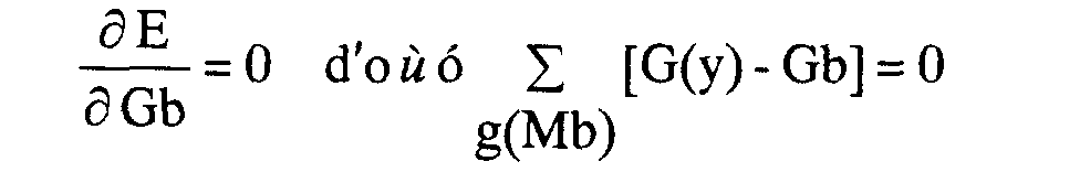


Cette formulation permet donc de déterminer immédiatement 2 des 5 paramètres annoncés précédemment : ces deux paramètres sont les niveaux d'intensité Ga et Gb représentant la hauteur du chapeau respectivement au centre, et de part et d'autre du centre du chapeau, en fonction du troisième paramètre qui est la largeur centrale La = (2a+1) du chapeau, et du quatrième paramètre qui est la largeur Lb = b de la partie externe du chapeau. On rappelle que pour cette première analyse du procédé, le cinquième paramètre yo a été figé dans une position particulière.This formulation therefore makes it possible to immediately determine 2 of the 5 previously announced parameters: these two parameters are the intensity levels Ga and Gb representing the height of the hat respectively in the center, and of share and from the center of the hat, depending on the third parameter which is the width central La = (2a + 1) of the hat, and of the fourth parameter which is the width Lb = b of the outer part of the hat. It will be recalled that for this first analysis of the process, the fifth parameter yo has been frozen in a particular position.
En portant maintenant dans l'équation 1b), les nouvelles expressions 2a)
et 2b) trouvées pour Ga et Gb, on arrive à une nouvelle expression de l'erreur E :
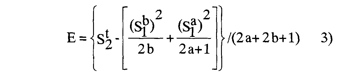
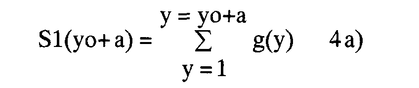


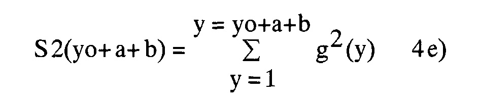
En référence à la FIG.3A, on considère que S t / 2 représente la différence entre la somme cumulée des intensités au carré dans l'intervalle des pixels entre le premier pixel de Δ et yo+a+b, et la somme cumulée des intensités au carré dans l'intervalle des pixels entre le premier pixel de Δ et yo-a-b-1. D'où il résulte que cet élément S t / 2 représente la somme cumulée des intensités des pixels, au carré, sur toute la longueur Lt du chapeau centré en yo, qui est considéré comme la position du pixel courant Pi fixé en yo pour cette étape du calcul.With reference to FIG. 3A, we consider that S t / 2 represents the difference between the cumulative sum of the squared intensities in the pixel interval between the first pixel of Δ and yo + a + b, and the cumulative sum of the squared intensities in the pixel interval between the first pixel of Δ and yo-a-b-1. Hence it follows that this element S t / 2 represents the cumulative sum of the intensities of the pixels, squared, over any the length Lt of the hat centered in yo, which is considered to be the position of the pixel current Pi set in yo for this step of the calculation.
En référence à la FIG.3B on considère que S a / 1 représente la différence entre la somme cumulée des intensités simples (c'est-à-dire non carrée) des pixels situés dans l'intervalle entre le premier pixel de Δ et yo+a, et la somme cumulée des intensités simples des pixels dans l'intervalle entre le premier pixel de Δ et yo-a-1.With reference to FIG.3B we consider that S a / 1 represents the difference between the cumulative sum of the simple (i.e. non-square) intensities of the pixels located in the interval between the first pixel of Δ and yo + a, and the cumulative sum of the intensities single pixels in the interval between the first pixel of Δ and yo-a-1.
En référence à la FIG.3C on considère que S b 2 / 1 représente la différence entre la somme cumulée des intensités simples des pixels situés dans l'intervalle entre le premier pixel de Δ et yo+a+b, et la somme cumulée des intensités simples dans l'intervalle entre le premier pixel de Δ et yo+a.With reference to FIG. 3C we consider that S b 2/1 represents the difference between the cumulative sum of the simple intensities of the pixels located in the interval between the first pixel of Δ and yo + a + b, and the cumulative sum of the simple intensities in the interval between the first pixel of Δ and yo + a.
En référence à la FIG.3D, on considère que S b1 / 1 représente la différence entre la somme cumulée des intensités simples des pixels situés dans l'intervalle entre le premier pixel de Δ et yo-a-1, et la somme cumulée des intensités simples des pixels situés dans l'intervalle entre le premier pixel de ▵ et yo-a-b-1.With reference to FIG. 3D, it is considered that S b1 / 1 represents the difference between the cumulative sum of the simple intensities of the pixels located in the interval between the first pixel of Δ and yo-a-1, and the cumulative sum of the intensities simple pixels located in the interval between the first pixel of ▵ and yo-a-b-1.
Ainsi pour calculer l'erreur quadratique E, il suffit en réalité de calculer une fois pour toute la somme cumulée des intensités simples ou la somme cumulée des intensités au carré pour tous les pixels de la droite de balayage ▵ (ou tous les points ayant des intensités interpolées éventuellement), et de réaliser les soustraction et addition indiquées dans les relations 5a), 5b), 5c), 5d), 5e) pour aboutir à la relation 3) donnant la nouvelle expression de l'erreur quadratique E.So to calculate the quadratic error E, it is really enough to calculate once for all the cumulative sum of simple intensities or the cumulative sum of squared intensities for all pixels of the scanning line ▵ (or all points having intensities possibly interpolated), and performing the subtraction and addition indicated in relations 5a), 5b), 5c), 5d), 5e) to arrive at relation 3) giving the new expression of the quadratic error E.
Cependant il faut prendre en compte que l'on cherche à réaliser les calculs de la manière la plus simple et la plus rapide possible. On cherche donc à minimiser le nombre des paramètres entrant dans cette relation 3) de E.However, we must take into account that we are trying to achieve the calculations in the simplest and fastest way possible. So we are looking to minimize the number of parameters entering into this relation 3) of E.
A cet effet, dans une première méthode, on fixe A PRIORI la largeur totale du chapeau Lt égale à une constante en pixels. Donc Lt = La + Lb = (2a+1)+2b pixels est fixe ; la longueur La de la partie centrale du chapeau est variable ; et la largeur "b" des bords du chapeau s'adapte en fonction du paramètre "a" pour que la largeur Lt reste fixe.To this end, in a first method, we set A PRIORI the width total of the hat Lt equal to a constant in pixels. So Lt = La + Lb = (2a + 1) + 2b pixels is fixed; the length La of the central part of the hat is variable; and the width "b" of the edges of the hat adapts according to the parameter "a" so that the width Lt remains fixed.
Dans ces conditions, il reste que :
Puisque l'on a maintenant fixé Lt, il reste seulement à déterminer la valeur de "a" qui minimise l'erreur quadratique exprimée par la formule 3).Since we have now fixed Lt, it only remains to determine the value of "a" which minimizes the quadratic error expressed by the formula 3).
Puisque l'on a fixé le paramètre Lt = 2a+2b+1, il en résulte que dans la
formule 3) le terme S t / 2 est une constante. Ce qui fait que pour minimiser l'erreur E de la
formule 3) il suffit de maximiser la fonction suivante V(a) :
Mais l'homme du métier peut décider que les variations appliquées à la valeur "a" peuvent avoir des limites. On peut par exemple se fixer que l'on ne cherche pas à détecter les branches ou objets dont la largeur est supérieure à 50 pixels.However, a person skilled in the art can decide that the variations applied to the value "a" may have limits. We can for example fix ourselves that we are not looking not detect branches or objects whose width is greater than 50 pixels.
En effet, comme représentée sur la FIG.1A, la ligne de balayage A3 peut couper une branche telle que 5 dont la direction générale est parallèle à cette ligne de balayage. Dans ce cas, on ne cherche pas à déterminer la largeur découpée par A3 sur cette branche 5, mais on effectuera ultérieurement des balayages selon une autre direction, par exemple parallèles à la ligne B1 qui est perpendiculaire à A3, pour déterminer la largeur de la section I5 qui est réellement intéressante pour les applications médicales envisagées.Indeed, as shown in FIG.1A, the scanning line A3 can cut a branch such as 5 whose general direction is parallel to this line of scanning. In this case, we are not trying to determine the width cut by A3 on this branch 5, but we will later carry out scans according to another direction, for example parallel to the line B1 which is perpendicular to A3, for determine the width of section I5 which is really interesting for applications medical plans.
Il faut souligner que, dans la phase d'analyse, on est parti de l'hypothèse
que le pixel courant Pi était déjà en yo à la fois centre de l'objet à déterminer et centre
du chapeau idéalement placé, d'où il résultait que la demi largeur a(yo) trouvée était
aussi la demi largeur de l'objet cherchée. Maintenant, il faut souligner que, dans la mise
en oeuvre du procédé selon l'invention, la détermination de la position du centre yo de
l'objet est précisément l'objet du procédé, ainsi que la détermination de la demi largeur
a(yo). C'est pourquoi, dans cette première méthode, le procédé selon l'invention va
comprendre plusieurs étapes.
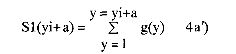
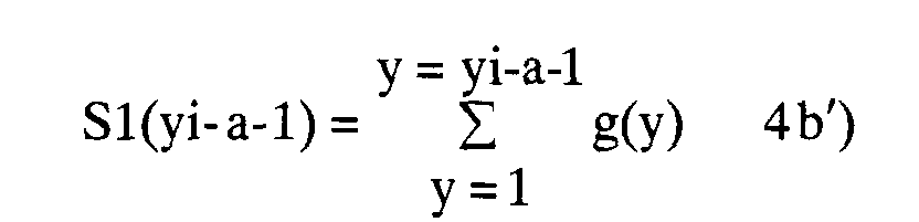

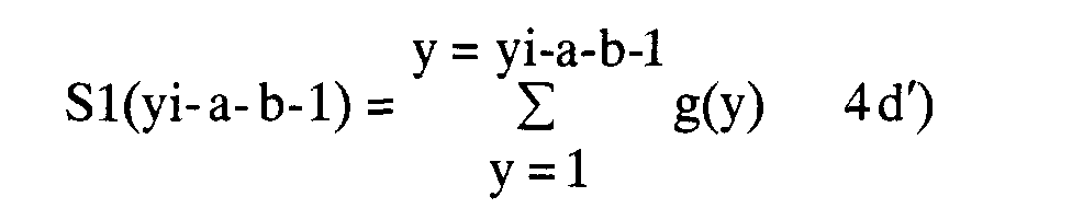
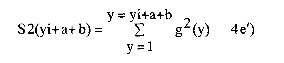
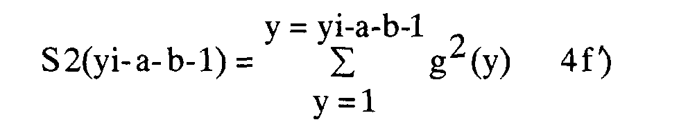
Cependant, cette première méthode présente un défaut dans le cas où il se trouve, dans l'image numérique à traiter, des branches ou des objets séparés l'un de l'autre par un nombre de pixels faible, quelques pixels. En effet, il apparaít que, dans ce cas, l'erreur E est minimisée lorsque le chapeau est positionné à cheval sur les deux pics des profils d'intensité qui résultent de cette situation lors du balayage de l'image ; cela est le cas d'un balayage représenté particulièrement par la ligne A2 de la FIG.1A, les profils d'intensité correspondant étant représentés sur la FIG.2B. Donc, dans la situation de la FIG.2B, l'erreur est minimisée lorsque le chapeau encadre les deux pics d'intensité, alors que si le chapeau est centré sur l'un ou l'autre des deux pics, l'erreur est très grande. However, this first method has a defect in the event that it there are, in the digital image to be processed, branches or separate objects one of the other by a small number of pixels, a few pixels. Indeed, it appears that in this case, the error E is minimized when the hat is positioned astride the two peaks intensity profiles that result from this situation when scanning the image; that is the case of a scan represented particularly by the line A2 of FIG.1A, the corresponding intensity profiles being shown in FIG.2B. So in the situation from FIG. 2B, the error is minimized when the hat frames the two intensity peaks, whereas if the hat is centered on one or the other of the two peaks, the error is very big.
Il en résulte que cette première méthode décrite ne permet pas de distinguer deux vaisseaux très rapprochés. C'est pourquoi une seconde méthode est proposée.It follows that this first method described does not allow distinguish two closely spaced vessels. This is why a second method is proposed.
Selon cette seconde méthode, au lieu de fixer la largeur totale Lt = La +
Lb du chapeau, pour le calcul de l'énergie de l'erreur, on fixe la dimension Lb du bord du
chapeau. Dans ces conditions, on pourra faire varier la largeur La de la partie centrale du
chapeau et en déduire la dimension totale Lt puisque la dimension du bord Lb ne
changera pas. Cette dimension Lb choisie pour le bord, qui peut être de quelques pixels,
va définir la résolution de cette deuxième méthode, puisque c'est cette dimension qui
permet de définir la distance minimale que peuvent avoir deux branches de la structure
arborescente entre elles pour être distinguées l'une de l'autre, ou deux objets de l'image
numérique. Si l'on a choisi une largeur Lb = 2 ou 3 pixels, on a ainsi défini que des
branches distantes de 2 ou 3 pixels pourront être distinguées. En fait le choix de Lb
résulte d'un compromis entre résolution et robustesse au bruit. Ainsi Lb = 1 pixel
donnerait la résolution maximale mais une robustesse au bruit inférieure. Ensuite, on
choisit un modèle, ou chapeau, de largeur centrale La variable. Cependant, pour limiter la
masse des calculs à effectuer, on reprend dans cette seconde méthode l'idée exposée
dans la première méthode qui consiste à exprimer l'énergie de l'erreur E en fonction des
sommes cumulées des intensités effectuées le long de la ligne de balayage considérée Δ.
Selon l'invention, on a vu qu'il suffit de calculer ces sommes cumulées une fois pour
toute, le long de chacune des lignes de balayage choisie. L'ensemble des calculs relatifs à
cette seconde méthode est exactement le même que pour la première méthode jusqu'à
l'expression de l'erreur en 3) :

Comme dans la première méthode précédemment décrite, on cherche à
déterminer la position yo du centre d'un objet coupé selon un segment I par une droite
de balayage Δ dans l'image numérique, ainsi que les points d'extrémité α, β de ce
segment, c'est-à-dire sa demi-largeur a(yo). C'est pourquoi le procédé dans cette
seconde méthode comprend les étapes suivantes :
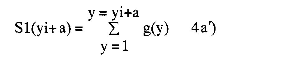
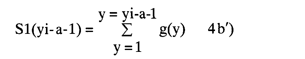
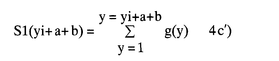

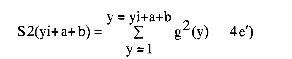

Ce test consiste à réaliser une étape de calculs dans laquelle on
détermine :
Ga(yo) et Gb(yo) 9) d'après les relations 7a), 7b) ou 8a), 8b). On décide que
l'optimum calculé selon la première ou la seconde méthode V(yo) ou E(yo) n'est pas
significatif d'un objet à prendre en compte ou à retenir,
Ga (yo) and Gb (yo) 9) according to the relations 7a), 7b) or 8a), 8b). We decide that the optimum calculated according to the first or second method V (yo) or E (yo) is not significant of an object to take into account or to remember,
La FIG.6A montre un diagramme schématique de blocs représentant des
moyens pour mettre en oeuvre le procédé décrit plus haut. En référence à la FIG.6A, on a
représenté un arrangement qui permet de procéder au traitement d'une image, laquelle
comporte la représentation d'au moins un objet OBJ constitué de pixels d'intensité
sensiblement uniforme, contrastant sur un fond BG constitué de pixels d'intensité
sensiblement uniforme comme montré sur la FIG.6B. Cet arrangement comprend :
En référence à la FIG.6A, cet arrangement comprend en outre :
- des moyens pour déterminer une fonction E(a,yi), V(a,yi) référencée première fonction desdites sommes cumulées mémorisées Σ, relatives aux intervalles sur la droite de balayage Δ, dont les pixels extrémités ont une abscisse définie par l'abscisse yi du pixel courant et par le paramètre de demi-largeur a,
- des moyens pour estimer une valeur optimale particulière E(yi), V(yi) de ladite première fonction relative au pixel courant Pi dans les limites (a1, am) dudit paramètre de demi largeur, comme montré sur les FIG.4A et FIG.5A. La seconde fonction des sommes cumulées étant ensuite construite en utilisant ces valeurs optimales particulières E(yi), V(yi), issues des seconds moyens de calcul 62 et relatives à tous les pixels de l'ensemble des pixels de la droite de balayage ▵.
- means for determining a function E (a, yi), V (a, yi) referenced first function of said accumulated sums stored Σ, relating to the intervals on the scanning line Δ, whose end pixels have an abscissa defined by the abscissa yi of the current pixel and by the half-width parameter a,
- means for estimating a particular optimal value E (yi), V (yi) of said first function relating to the current pixel Pi within the limits (a1, am) of said half-width parameter, as shown in FIGS. 4A and FIG. 5A. The second function of the cumulative sums then being constructed using these particular optimal values E (yi), V (yi), coming from the second calculation means 62 and relating to all the pixels of the set of pixels of the scanning line ▵ .
La FIG.6C représente schématiquement le résultat obtenu en sortie des quatrièmes moyens de stockage MEM4, c'est-à-dire l'abscisse sur la droite ▵, dans l'image, du centre de l'objet, et les deux demi-largeurs a(yo) de part et d'autre du centre, permettant d'apprécier le segment I. L'arrangement de la FIG.6A permet de traiter toutes les droites de balayage voulues pour délimiter les centres et bords d'un objet OBJ avec précision.FIG. 6C schematically represents the result obtained at the output of fourth MEM4 storage means, i.e. the abscissa on the line ▵, in the image, from the center of the object, and the two half-widths a (yo) on either side of the center, allowing to appreciate the segment I. The arrangement of FIG. 6A makes it possible to treat all the scanning lines you want to delimit the centers and edges of an OBJ object with precision.
Claims (13)
- A method of processing an image which includes the representation of at least one object (OBJ) consisting of pixels of substantially uniform intensity contrasted against a background (BG) consisting of pixels of substantially uniform intensity, this method comprising:the determination of at least one image scan trace (Δ) formed by a set of adjacent pixels and the determination of a segement (I) formed by said trace cutting said object of the image;the computation and storage of the cumulated sums of the intensities and of the squared intensities of the adjacent pixels over all the intervals of the trace which are delimited by an origin pixel (y1), on the one hand, and by each of the pixels, respectively, of said set of pixels, labelled end pixels, on the other;the construction, over said set of pixels of the trace, of a function [E(yi), V(yi)] of said cumulated sums, labelled second function, and said construction comprising the formulation, by means of said stored cumulated sums, of the quadratic error function between a real intensity function [g9Y0] of the pixels over the set of the pixels of the scan trace and an intensity function [M(y)] of a binary model which come nearest to the profile of the real intensity function [g(y)];the estimation of the optimal value [E(yo), V(yo)] of said second function;and the estimation of the centre (yo) and of the semi-width [a(yo)] of said segment (I) of the trace (Δ), as, respectively, the value of the abscissa (yo) of a pixel of said trace, and the value [a(yo)] of a parameter (a) labelled semi-width parameter which yield said optimal value [E(yo), V(yo)] of said second function.
- A method as claimed in Claim 1, characterized in that, for the construction of said second function of the cumulated sums [E(yi), V(yi)] over said set of pixels, it comprises:the definition of a parameter (a) labelled semi-width parameter, evaluated as a number of pixels variable between limits (a1, am);the processing of each of the pixels of said set over the trace, in a scan direction starting from said origin pixel (y1) with, for each current pixel (Pi), defined by its abscissa (yi) on the trace:the determination of a function [E(a,yi), V(a,yi)] of said stored cumulated sums, labelled first function, relating to said intervals on the trace, the end pixels of which have an abscissa defined by the abscissa (yi) of the current pixel and by the semi-width parameter (a),the estimation of the particular optimal value [E(yi), V(yi)] of said first function relating to said current pixel (Pi) within the limits (a1, am) of said semi-width parameter, and in that in the construction of said second function of the cumulated sums [E(yi), V(yi)], this second function consists of a function of said particular optimal values [E(yi), V(yi)].
- An image processing method as claimed in Claim 2, characterized in that the determination of said first function [E(a,yi), V(a,yi)] of the cumulated sums comprises:said model being centred on the current pixel (Pi) defined by its abscissa (yi) on said trace, for each value of the semi-width parameter (a) varying within its limits (a1, am), and these cumulated sums being expressed by differences between said cumulated sums of the simple or squared intensities of the pixels computed over all the intervals of the scan trace which are limited, on the one hand, by said origin pixel (y1) and, on the other, by said end pixels consisting of the edge pixels of the first and second portions of the model.the definition of a rectangular intensity model (M(y)) over said scan trace having a first central portion (Ma) of semi-width measured in pixels equal to the value of said semi-width parameter (a); two second outer portions (Mb1, Mb2) symmetrically flanking the first central portion, of width measured in pixels labelled outer width parameter (b),and the estimation, at said current pixel (Pi) of the cumulated sums of the squared intensities (S2 t) of the pixels over the total width (Lt = 2a + 2b + 1) of the model, of the intensities of the pixels (S1 a) over the first central portion (Ma) of the model, and of the intensities of the pixels (S1 b) over each of the second outer portions (Mb1, Mb2) of the model,
- An image processing method as claimed in Claim 3, characterized in that the rectangular intensity model over the scan trace is furthermore defined by:a first constant intensity (Ga) over the extent of said first central portion,a second constant intensity (Gb), within each of the second outer portions (Mb1, Mb2), the difference of the first and second intensities having the sign of the difference of the intensities between said object and said background of the digital image, and in that the determination of said first function [E(a,yi), V(a,yi)] of the cumulated sums comprises the formulation, by means of said stored cumulated sums, of the function of the quadratic error between the actual intensity function [g(y)] of the pixels over said set of pixels of the scan trace, and the intensity function [Ga, Gb] of the rectangular model.
- A method as claimed in Claim 4, characterized in that the function of the quadratic error between the actual intensity function (g(y)) and the intensity function of the model (M(y)) is expressed by said first function:with

- A method as claimed in Claim 5, characterized in that the width parameter of the two outer portions (Mb1, Mb2) of the model is a constant in the formulation of the quadratic error function and in that the estimation of the particular optimal value [E(yi)] of said first function relating to said current pixel (Pi) is carried out by minimization of said function.
- A method as claimed in Claim 5, characterized in that the total width parameters (Lt) of the model are a constant in the formulation of the quadratic error function and in that the estimation of the particular optimal value [E(yi)] of said first function relating to the current pixel is carried out by maximization of the function:
- A method as claimed in Claim 7, characterized in that the value of the width parameter (b) of the second outer portions of the model (Mb1, Mb2) determines the resolution of the method and is for this purpose chosen to be less than 10 pixels as a compromise with the robustness to noise.
- A method as claimed in one of Claims 6, 7 or 8, characterized in that it furthermore comprises the fixing of thresholds so as to process in the digital image only significant objects, said thresholds including first types of thresholds imposed on said optimal values [E(yo), V(yo)] of the error function corresponding to the ordinate of the centre (yo) determined for one of said potentially significant objects, and second types of thresholds imposed on the difference between the two intensity levels (Ga, Gb) of the rectangular model (M(y)) centred at this abscissa (yo) of the centre of said object.
- A method as claimed in one of the preceding claims, characterized in that the value of the semi-width parameter (a) is between 5 and 50 pixels, and in that the scan interval [yl,yn] for the current pixel (yi) on a trace (Δ) is between 50 and 1,000 pixels.
- A method as claimed in one of the preceding claims, characterized in that the directions of the scan traces are arbitrary, and that in this case, this method comprises:the defining of points on these traces with regularly distributed abscissae (yi),and the computation of the intensity at each point by a method of interpolation as a function of the intensities of the pixels of a given neighborhood about each point, optionally assigning the intensities of these neighboring pixels a weight which decreases the further these pixels are away from the relevant point.
- An arrangement for processing an image including the representation of at least one object (OBJ) consisting of pixels of substantially uniform intensity contrasted against a background (BG) consisting of pixels of substantially uniform intensity, this arrangement comprising:storage means (51) labelled first storage means (MEM1) for storing image data of said image and for providing a trace (Δ) scanning said image, said scan trace being formed by a set of adjacent pixels and cutting said object (OBJ) of the image in a segment (I);computing means (61) labelled first computing means (CMP1) for computing cumulated sums (∑) of the intensities and squared intensities of adjacent pixels over all the intervals of said scan trace (Δ), these intervals being limited by a first pixel labelled origin pixel (y1), on the one hand, and, respectively, each one of the pixels of said set of pixels, labelled the end pixels, on the other;storage means (52) labelled second storage means (MEM2) for storing the output data of said first computing means (61);computing means (63) labelled third computing means (CMP3) for constructing, on said set of pixels of the scan trace (Δ), a function of said cumulated sums labelled second function [E(yi), V(yi)] said construction comprising the formulation, by means of said stored cumulated sums, of the quadratic error function between a real intensity function [g9Y0] of the pixels over the set of the pixels of the scan trace and an intensity function [M(y)] of a binary model which come nearest to the profile of the real intensity function [g(y)]; and for further estimating an optimal value [E(yo), V(yo)] of said second function constructed relative to said set of pixels of the trace;storage means (54) labelled fourth storage means (MEM4) for storing a value of the abscissa (yo) of a pixel of the scan trace (Δ), and a value [a(yo)] of a parameter (a) labelled semi-width parameter, to constitute the abscissa of the centre (yo), and the semi-width [a(yo)] of said segment (I) determined by said trace (Δ), cutting said object (OBJ) of the image, as, respectively, the values which yield said optimal value [E(yo), V(yo)] of said second function of the cumulated sums, constructed by said third computing means;display means for displaying said image, having a two-dimensional matrix of pixels.
- An arrangement as claimed in Claim 12, further comprising:said second function of the cumulated sums then being constructed by using said particular optimal values [E(yi), V(yi)] issued of said second computing means (62), and related to all pixels of the set of pixels of the scan trace (Δ).storage means (53) labelled third storage means (MEM3) for storing a parameter (a) labelled semi-width parameter, said parameter being evaluated as a number of pixels variable between two limits (a1, am);computing means (62), labelled second computing means (CMP2), for processing each pixel, labelled current pixel (Pi) defined by its abscissa (yi) on the scan trace (Δ), said second computing means (62) including:means for determining a function [E(a,yi), V(a,yi)] labelled first function of said stored cumulated sums (∑), relative to said intervals on the scan trace (Δ), of which the end pixels have an abscissa defined by the abscissa (yi) of the current pixel and by the semi-width parameter (a),means for computing a particular optimal value [E(yi), V(yi)] of said first function related to said current pixel (Pi) within the limits (a1, am) of said semi-width parameter,
Applications Claiming Priority (2)
| Application Number | Priority Date | Filing Date | Title |
|---|---|---|---|
| FR9401770 | 1994-02-16 | ||
| FR9401770 | 1994-02-16 |
Publications (2)
| Publication Number | Publication Date |
|---|---|
| EP0668570A1 EP0668570A1 (en) | 1995-08-23 |
| EP0668570B1 true EP0668570B1 (en) | 2001-09-26 |
Family
ID=9460143
Family Applications (1)
| Application Number | Title | Priority Date | Filing Date |
|---|---|---|---|
| EP95200303A Expired - Lifetime EP0668570B1 (en) | 1994-02-16 | 1995-02-08 | Image processing method for locally determining the center and half-length of contrasting objects on a background and apparatus to carry out the method |
Country Status (4)
| Country | Link |
|---|---|
| US (1) | US5771308A (en) |
| EP (1) | EP0668570B1 (en) |
| JP (1) | JPH07271976A (en) |
| DE (1) | DE69522844T2 (en) |
Families Citing this family (33)
| Publication number | Priority date | Publication date | Assignee | Title |
|---|---|---|---|---|
| US6151404A (en) * | 1995-06-01 | 2000-11-21 | Medical Media Systems | Anatomical visualization system |
| JP3363735B2 (en) * | 1996-06-26 | 2003-01-08 | 松下電器産業株式会社 | X-ray imaging device |
| DE19705599A1 (en) * | 1997-02-14 | 1998-08-20 | Philips Patentverwaltung | X-ray imaging process with a series of exposures from different perspectives |
| FR2764411B1 (en) * | 1997-06-09 | 1999-07-16 | Eastman Kodak Co | PROCESS FOR OPTIMIZING THE FILLING OF AN EDITING MEDIA WITH DIGITAL IMAGES OF VARIABLE SIZES, AND WITH CONSERVATION OF SIZE RELATIONSHIPS |
| US6636626B1 (en) | 1999-11-30 | 2003-10-21 | Wafermasters, Inc. | Wafer mapping apparatus and method |
| US6829379B1 (en) * | 2000-11-27 | 2004-12-07 | Ge Medical Systems Global Technology Company, Llc | Methods and apparatus to assist and facilitate vessel analysis |
| JP2005520350A (en) * | 2000-12-01 | 2005-07-07 | ウェーハマスターズ・インコーポレイテッド | Wafer mapping apparatus and method |
| AU2003247376A1 (en) * | 2002-05-17 | 2003-12-02 | Case Western Reserve University | Double contrast technique for mri-guided vascular interventions |
| DE10312193A1 (en) * | 2003-03-19 | 2004-09-09 | Siemens Ag | Operation of a medical diagnostic imaging unit, especially a computer tomography or magnetic resonance imaging instrument, whereby image data and segment data sets are processed and presented simultaneously |
| DE10319546A1 (en) | 2003-04-30 | 2004-11-25 | Siemens Ag | Automatic vein structure anomaly detection procedure recognises vein structure in tomography data, prepares skeletal path and classifies by comparison with characteristic values |
| US7697786B2 (en) * | 2005-03-14 | 2010-04-13 | Sarnoff Corporation | Method and apparatus for detecting edges of an object |
| US8004536B2 (en) * | 2006-12-01 | 2011-08-23 | Adobe Systems Incorporated | Coherent image selection and modification |
| US8175409B1 (en) | 2006-12-01 | 2012-05-08 | Adobe Systems Incorporated | Coherent image selection and modification |
| US7953266B2 (en) * | 2007-02-06 | 2011-05-31 | Siemens Medical Solutions Usa, Inc. | Robust vessel tree modeling |
| US9355469B2 (en) | 2009-01-09 | 2016-05-31 | Adobe Systems Incorporated | Mode-based graphical editing |
| US9232925B2 (en) * | 2011-04-22 | 2016-01-12 | Shimadzu Corporation | X-ray diagnostic apparatus and storage medium storing X-ray diagnostic program |
| DE102012214351B4 (en) * | 2012-08-13 | 2014-11-06 | Siemens Aktiengesellschaft | Angiographic examination procedure of a vascular system |
| US9002084B2 (en) * | 2013-08-30 | 2015-04-07 | Ge Medical Systems Israel, Ltd | Systems and methods for summing signals from an imaging detector |
| US9482764B1 (en) | 2015-05-28 | 2016-11-01 | General Electric Company | Systems and methods for charge-sharing identification and correction using a single pixel |
| US10156645B2 (en) | 2016-12-23 | 2018-12-18 | General Electric Company | Systems and methods for sub-pixel location determination at sidewalls and corners of detectors |
| US10145964B1 (en) | 2017-05-15 | 2018-12-04 | General Electric Company | Systems and methods for improved collimation sensitivity |
| US9983320B1 (en) | 2017-05-15 | 2018-05-29 | General Electric Company | Systems and methods for improved collimation sensitivity |
| US10324200B2 (en) | 2017-05-15 | 2019-06-18 | General Electric Company | Systems and methods for improved collimation sensitivity |
| EP3457353B1 (en) * | 2017-09-18 | 2020-11-25 | Siemens Healthcare GmbH | Method and system for obtaining a true shape of objects in a medical image |
| US10761224B2 (en) | 2018-06-06 | 2020-09-01 | General Electric Company | Systems and methods for improved detector assembly sizing |
| US10481285B1 (en) | 2018-08-13 | 2019-11-19 | General Electric Company | Systems and methods for determination of depth of interaction |
| US10976452B2 (en) | 2018-08-13 | 2021-04-13 | General Electric Medical Systems Israel, Ltd. (Il) | Systems and methods for improved medical imaging |
| US10247834B1 (en) | 2018-08-15 | 2019-04-02 | General Electric Company | Anodes for improved detection of non-collected adjacent signal |
| US10591619B2 (en) | 2018-08-15 | 2020-03-17 | GE Precision Healthcare LLC | Anodes for improved detection of non-collected adjacent signals |
| US11642172B2 (en) * | 2019-03-05 | 2023-05-09 | Biosense Webster (Israel) Ltd. | Showing catheter in brain |
| CN110796693B (en) * | 2019-09-11 | 2023-03-21 | 重庆大学 | Method for directly generating two-dimensional finite element model from industrial CT slice image |
| US11320545B2 (en) | 2020-07-07 | 2022-05-03 | GE Precision Healthcare LLC | Systems and methods for improved medical imaging |
| US11092701B1 (en) | 2020-07-07 | 2021-08-17 | GE Precision Healthcare LLC | Systems and methods for improved medical imaging |
Family Cites Families (5)
| Publication number | Priority date | Publication date | Assignee | Title |
|---|---|---|---|---|
| US4101961A (en) * | 1977-02-16 | 1978-07-18 | Nasa | Contour detector and data acquisition system for the left ventricular outline |
| FR2623642B1 (en) * | 1987-11-23 | 1990-03-09 | Thomson Rech | METHOD FOR SEGMENTATION OF VASCULAR ANGIOGRAPHIC IMAGES BY VECTOR TRACKING OF AXES AND CONTROLLED CONTOUR DETECTION |
| US5054094A (en) * | 1990-05-07 | 1991-10-01 | Eastman Kodak Company | Rotationally impervious feature extraction for optical character recognition |
| JP3057935B2 (en) * | 1992-11-16 | 2000-07-04 | ブラザー工業株式会社 | Character output device |
| FR2708166A1 (en) | 1993-07-22 | 1995-01-27 | Philips Laboratoire Electroniq | A method of processing digitized images for the automatic detection of stenoses. |
-
1995
- 1995-02-08 DE DE69522844T patent/DE69522844T2/en not_active Expired - Fee Related
- 1995-02-08 EP EP95200303A patent/EP0668570B1/en not_active Expired - Lifetime
- 1995-02-15 US US08/388,864 patent/US5771308A/en not_active Expired - Fee Related
- 1995-02-16 JP JP7028247A patent/JPH07271976A/en not_active Abandoned
Also Published As
| Publication number | Publication date |
|---|---|
| EP0668570A1 (en) | 1995-08-23 |
| JPH07271976A (en) | 1995-10-20 |
| DE69522844D1 (en) | 2001-10-31 |
| US5771308A (en) | 1998-06-23 |
| DE69522844T2 (en) | 2002-05-16 |
Similar Documents
| Publication | Publication Date | Title |
|---|---|---|
| EP0668570B1 (en) | Image processing method for locally determining the center and half-length of contrasting objects on a background and apparatus to carry out the method | |
| EP0635806A1 (en) | Method for processing digital pictures for locally determining centre and width of objects having the form of bands contrasting with background | |
| EP0840252B1 (en) | Digital image-processing method for the automatic extraction of ribbon-like objects | |
| EP0434508B1 (en) | Multi-scale reconstruction method of a body structure image | |
| EP0945830B1 (en) | Image processing method including multidimensional image segmentation stages and medical imaging apparatus using the same | |
| EP0379399B1 (en) | Process for calculating and evaluating a conically projected image, for example an X-ray image, of a three-dimensional sampled object, and process for the three-dimensional reconstruction of an object subject to above calculating process | |
| EP0720125B1 (en) | Image forming apparatus and method for correcting optical geometrical distortions in an image | |
| CA2491751C (en) | Method for processing an image acquired through a guide consisting of a plurality of optical fibers | |
| EP1756771B1 (en) | Fine stereoscopic image matching and dedicated instrument having a low stereoscopic coefficient | |
| EP3412245B1 (en) | Process for evaluating an orthodontic splint | |
| EP0822515A1 (en) | Automatic segmentation method for digital images and apparatus using such method | |
| EP0692772A1 (en) | Method and apparatus for detecting characteristic points on the contour of an object | |
| FR2885717A1 (en) | Mask digital image correction estimation method for angiography device, involves finding mobile region position for digital contrast detection images, where image correction is transformation of region from position to region of interest | |
| FR2641099A1 (en) | ||
| FR2731819A1 (en) | CONTOUR EXTRACTION METHOD USING MULTI-FRACTAL ANALYSIS | |
| EP0434720A1 (en) | Method for reconstructing a three-dimensional arborescence by labelling | |
| CN108369737A (en) | Using heuristic graph searching quickly and automatically to divide layered image | |
| EP0927953A1 (en) | Multidimensional noisy image processing method and medical imaging apparatus using this method | |
| EP1417646B1 (en) | Method for reconstruction of an image of an evolving object | |
| FR2819919A1 (en) | TRACKING THE DEFORMATION OF A LINEAR STRUCTURE ON AN IMAGE OF A SEQUENCE OF IMAGES OF A TIME-DEFORMABLE MEMBER | |
| EP3509483B1 (en) | System and method for reconstructing a physiological signal of an artery/tissue/vein dynamic system of an organ in a surface space | |
| EP3054422A1 (en) | Method for determining an axis of rotation of a tomography object and method for characterisation by tomography | |
| FR2910673A1 (en) | IMAGE PROCESSING METHOD AND DEVICE IMPLEMENTING SAID METHOD | |
| FR2831306A1 (en) | Medical imaging station with rapid image segmentation has segmentation means for processing gray level images, with means for adjusting front propagation speed so that local zero values can be created | |
| FR2997284A1 (en) | METHOD FOR OBTAINING TOMOSYNTHESIS IMAGES |
Legal Events
| Date | Code | Title | Description |
|---|---|---|---|
| PUAI | Public reference made under article 153(3) epc to a published international application that has entered the european phase |
Free format text: ORIGINAL CODE: 0009012 |
|
| AK | Designated contracting states |
Kind code of ref document: A1 Designated state(s): DE FR GB NL |
|
| RAP1 | Party data changed (applicant data changed or rights of an application transferred) |
Owner name: PHILIPS ELECTRONICS N.V. Owner name: LABORATOIRES D'ELECTRONIQUE PHILIPS S.A.S. |
|
| 17P | Request for examination filed |
Effective date: 19960223 |
|
| 17Q | First examination report despatched |
Effective date: 19990525 |
|
| RAP1 | Party data changed (applicant data changed or rights of an application transferred) |
Owner name: KONINKLIJKE PHILIPS ELECTRONICS N.V. |
|
| GRAG | Despatch of communication of intention to grant |
Free format text: ORIGINAL CODE: EPIDOS AGRA |
|
| GRAG | Despatch of communication of intention to grant |
Free format text: ORIGINAL CODE: EPIDOS AGRA |
|
| GRAH | Despatch of communication of intention to grant a patent |
Free format text: ORIGINAL CODE: EPIDOS IGRA |
|
| GRAH | Despatch of communication of intention to grant a patent |
Free format text: ORIGINAL CODE: EPIDOS IGRA |
|
| GRAA | (expected) grant |
Free format text: ORIGINAL CODE: 0009210 |
|
| AK | Designated contracting states |
Kind code of ref document: B1 Designated state(s): DE FR GB NL |
|
| PG25 | Lapsed in a contracting state [announced via postgrant information from national office to epo] |
Ref country code: NL Free format text: LAPSE BECAUSE OF FAILURE TO SUBMIT A TRANSLATION OF THE DESCRIPTION OR TO PAY THE FEE WITHIN THE PRESCRIBED TIME-LIMIT Effective date: 20010926 Ref country code: GB Free format text: LAPSE BECAUSE OF FAILURE TO SUBMIT A TRANSLATION OF THE DESCRIPTION OR TO PAY THE FEE WITHIN THE PRESCRIBED TIME-LIMIT Effective date: 20010926 |
|
| REF | Corresponds to: |
Ref document number: 69522844 Country of ref document: DE Date of ref document: 20011031 |
|
| NLV1 | Nl: lapsed or annulled due to failure to fulfill the requirements of art. 29p and 29m of the patents act | ||
| GBV | Gb: ep patent (uk) treated as always having been void in accordance with gb section 77(7)/1977 [no translation filed] |
Effective date: 20010926 |
|
| PLBE | No opposition filed within time limit |
Free format text: ORIGINAL CODE: 0009261 |
|
| STAA | Information on the status of an ep patent application or granted ep patent |
Free format text: STATUS: NO OPPOSITION FILED WITHIN TIME LIMIT |
|
| 26N | No opposition filed | ||
| REG | Reference to a national code |
Ref country code: FR Ref legal event code: D6 |
|
| PGFP | Annual fee paid to national office [announced via postgrant information from national office to epo] |
Ref country code: FR Payment date: 20030224 Year of fee payment: 9 |
|
| PGFP | Annual fee paid to national office [announced via postgrant information from national office to epo] |
Ref country code: DE Payment date: 20030416 Year of fee payment: 9 |
|
| PG25 | Lapsed in a contracting state [announced via postgrant information from national office to epo] |
Ref country code: DE Free format text: LAPSE BECAUSE OF NON-PAYMENT OF DUE FEES Effective date: 20040901 |
|
| PG25 | Lapsed in a contracting state [announced via postgrant information from national office to epo] |
Ref country code: FR Free format text: LAPSE BECAUSE OF NON-PAYMENT OF DUE FEES Effective date: 20041029 |
|
| REG | Reference to a national code |
Ref country code: FR Ref legal event code: ST |