WO2024259419A2 - Motor control using optimal efficiency reference generation - Google Patents

Motor control using optimal efficiency reference generation Download PDF

Info

Publication number
WO2024259419A2
WO2024259419A2 PCT/US2024/034328 US2024034328W WO2024259419A2 WO 2024259419 A2 WO2024259419 A2 WO 2024259419A2 US 2024034328 W US2024034328 W US 2024034328W WO 2024259419 A2 WO2024259419 A2 WO 2024259419A2
Authority
WO
WIPO (PCT)
Prior art keywords
motor
control parameter
reference frame
function
model
Prior art date
Legal status (The legal status is an assumption and is not a legal conclusion. Google has not performed a legal analysis and makes no representation as to the accuracy of the status listed.)
Ceased
Application number
PCT/US2024/034328
Other languages
French (fr)
Other versions
WO2024259419A3 (en
Inventor
Matthias PREINDL
Bernard William STEYAERT
Ethan Bagget SWINT
Walter Wesley PENNINGTON III
Current Assignee (The listed assignees may be inaccurate. Google has not performed a legal analysis and makes no representation or warranty as to the accuracy of the list.)
Columbia University in the City of New York
Tau Motors Inc
Original Assignee
Columbia University in the City of New York
Tau Motors Inc
Priority date (The priority date is an assumption and is not a legal conclusion. Google has not performed a legal analysis and makes no representation as to the accuracy of the date listed.)
Filing date
Publication date
Application filed by Columbia University in the City of New York, Tau Motors Inc filed Critical Columbia University in the City of New York
Priority to KR1020267001514A priority Critical patent/KR20260046084A/en
Priority to EP24824347.9A priority patent/EP4728634A2/en
Publication of WO2024259419A2 publication Critical patent/WO2024259419A2/en
Publication of WO2024259419A3 publication Critical patent/WO2024259419A3/en
Anticipated expiration legal-status Critical
Ceased legal-status Critical Current

Links

Classifications

    • HELECTRICITY
    • H02GENERATION; CONVERSION OR DISTRIBUTION OF ELECTRIC POWER
    • H02PCONTROL OR REGULATION OF ELECTRIC MOTORS, ELECTRIC GENERATORS OR DYNAMO-ELECTRIC CONVERTERS; CONTROLLING TRANSFORMERS, REACTORS OR CHOKE COILS
    • H02P21/00Arrangements or methods for the control of electric machines by vector control, e.g. by control of field orientation
    • H02P21/0085Arrangements or methods for the control of electric machines by vector control, e.g. by control of field orientation specially adapted for high speeds, e.g. above nominal speed
    • HELECTRICITY
    • H02GENERATION; CONVERSION OR DISTRIBUTION OF ELECTRIC POWER
    • H02PCONTROL OR REGULATION OF ELECTRIC MOTORS, ELECTRIC GENERATORS OR DYNAMO-ELECTRIC CONVERTERS; CONTROLLING TRANSFORMERS, REACTORS OR CHOKE COILS
    • H02P25/00Arrangements or methods for the control of AC motors characterised by the kind of AC motor or by structural details
    • H02P25/02Arrangements or methods for the control of AC motors characterised by the kind of AC motor or by structural details characterised by the kind of motor
    • H02P25/022Synchronous motors

Definitions

  • a synchronous motor is an alternating current (AC) motor having a stator that is driven by AC supply signals (e.g., one signal for each phase of the stator) to cause rotation of a rotor.
  • AC supply signals e.g., one signal for each phase of the stator
  • the AC supply signals in stator windings of the stator generate magnetic fields that interact with a magnetic field or fields of the rotor to cause rotation of the rotor.
  • the rotation of the rotor is generally synchronous with the frequency of the AC supply current.
  • the rotor may be a permanent magnet rotor, a wound field rotor, or a hybrid rotor including both wound fields and permanent magnets. In the case of a permanent magnet rotor, one or more permanent magnets of the rotor generate the magnetic field or fields of the rotor.
  • a motor controller may control an inverter to provide an AC signal to each phase of the motor based on current rotor position and other -1- Q B ⁇ 175073.00216 ⁇ 90201874.3 Attorney Docket No.: 175073.00216 characteristics of the motor.
  • the physics of the magnetic fields of each stator winding interacting with the rotating rotor can lead to complex mathematics problems that are challenging to create and solve to address factors that lead to efficient driving of the motor, and these challenges can be exacerbated in the case of a wound field synchronous (WFS) motor because of the added wound field rotor.
  • WFS wound field synchronous
  • a WFS motor may also be referred to as WFS machine, a wound rotor synchronous machine (WRSM), a wound field synchronous machine (WFSM), a wound rotor synchronous generator (WRSG), a wound field synchronous generator (WFSG), as well as several other names.
  • WFS machine as a power-dense, permanent magnet free, synchronous machine, has gained significant interest in recent years in the field of transportation electrification.
  • a motor controller for a WFS machine may receive a control input, e.g., a reference current or flux, and control the motor in an attempt to achieve an actual motor current or flux that matches the reference current or flux.
  • the control input may be generated by a reference generation map (or reference map).
  • the reference map may itself receive a control input (e.g., a reference torque (T*) or reference motor speed ( ⁇ *), for example, from a user input (e.g., accelerator pedal or other throttle or torque control) or memory. Based on this control input (e.g., T* or ⁇ *), the reference map may generate as output the control input for the motor controller (or an intermediate value that is further translated to the control input).
  • a control input e.g., a reference torque (T*) or reference motor speed ( ⁇ *)
  • T* or ⁇ * reference torque
  • the reference map may generate as output the control input for the motor controller (or an intermediate value that is further translated to the control input).
  • reference generation maps for electric machines may take some combination of torque and/or speed and output a set of currents that attempt to minimize the electrical losses of the machine.
  • the ability to control the machine at high efficiency by using as a reference map either a static map (like a maximum torque per ampere (MTPA) map) or a dynamic optimization problem (like direct torque model predictive control (MPC)) use both loss models of the machine and a mechanism to operate the efficiency map in real time.
  • the dominant losses are copper loss and core loss, which are generally proportional to torque and speed, respectively.
  • the integration of core losses into a reference map is generally neglected in literature because of computational complexity and domination of copper losses over core losses.
  • reference maps may output reference values (e.g., current or flux values) that do not minimize losses, particularly at higher motor speeds where core losses can increase.
  • OERG optimal efficiency reference generation
  • the OERG-based control is based on an optimization problem (or cost function) that uses a convex loss function. Coefficients of the loss function may be determined using finite element analysis (FEA) data, and may be solved over a wide range of inputs (e.g., torques and speeds), showing different output trajectories (e.g., current trajectories).
  • FFA finite element analysis
  • Machine design engineers may design machines to minimize their core loss by analyzing the effects of eddy currents, hysteresis, and armature reaction effects with different geometries, materials, and laminations. For WFS machines, this can be important as its primary application until recently has been larger, megavolt-ampere (MVA)-sized machines for power generation.
  • MVA megavolt-ampere
  • WFS machines have seen a recent increase in popularity in automotive applications, as a WFS machine is a compromise between two popular machines types in the space: a high power density permanent magnet synchronous machine (PMSM) that may be efficient but expensive, and low power density induction machine (IM) that may be cheap but inefficient.
  • PMSM permanent magnet synchronous machine
  • IM low power density induction machine
  • Some WFS machines use hairpin windings to increase slot fill factor; but, this approach increases core losses and introduces additional manufacturing complexity.
  • -3- Q B ⁇ 175073.00216 ⁇ 90201874.3 Attorney Docket No.: 175073.00216 [0011] It may be desirable, particularly in automotive applications, for machines to operate efficiently for a wide range of speed and torque.
  • the proposed models have 12% and 53% average error when compared to FEA.
  • the two models use just 15 and 12 floating point operations each, and use 9 or 729 coefficients each.
  • Example use-cases of the two models are maximum efficiency point selection, real-time control, and FEA outlier detection.
  • some embodiments provided herein are directed to OERG-based motor control.
  • OERG-based motor control that use one of the core loss models described herein.
  • OERG-based motor control is also applicable to other motor types, including other permanent magnet motors, brushless motors with permanent magnet rotors, induction motors, universal motors, reluctance motors (synchronous and switched), and the like.
  • an electric machine serving as an electric motor that outputs mechanical power from input electric power may also operate in reverse and serve as an electric generator that outputs electric power from input mechanical power.
  • a motor system includes a power switching network configured to be coupled to a power supply and to a motor; and an electronic controller.
  • the electronic controller is configured to: determine current values for the motor in a rotational reference frame, each current value associated with a dimension of a set of dimensions -4- Q B ⁇ 175073.00216 ⁇ 90201874.3 Attorney Docket No.: 175073.00216 of the rotational reference frame; determine, based on a desired control parameter, a target motor control parameter value for each dimension of the set of dimensions of the rotational reference frame using an optimization cost function that considers motor speed, copper loss, and core loss; and control the power switching network based on the current values and the target motor control parameter values.
  • a method of controlling a motor is provided.
  • the method includes: determining, by an electronic controller, current values for a motor in a rotational reference frame, each current value associated with a dimension of a set of dimensions of the rotational reference frame; determining, by the electronic controller and based on a desired control parameter, a target motor control parameter value for each dimension of the set of dimensions of the rotational reference frame using an optimization cost function that considers motor speed, copper loss, and core loss; and controlling, by the electronic controller, a power switching network based on the current values and the target motor control parameter values.
  • a non-transitory computer-readable medium storing computer- executable instructions, where the instructions are for causing a processor to: determine current values for a motor in a rotational reference frame, each current value associated with a dimension of a set of dimensions of the rotational reference frame; determine, based on a desired control parameter, a target motor control parameter value for each dimension of the set of dimensions of the rotational reference frame using an optimization cost function that considers motor speed, copper loss, and core loss; and control a power switching network coupled to the motor based on the current values and the target motor control parameter values.
  • FIG.1 illustrates a motor system according to some embodiments. -5- Q B ⁇ 175073.00216 ⁇ 90201874.3 Attorney Docket No.: 175073.00216 [0020]
  • FIG. 2 illustrates a motor control system implementing optimal efficiency reference generation (OERG) according to some embodiments.
  • OERG optimal efficiency reference generation
  • FIG. 3 illustrates a process for implementing OERG-based motor control according to some embodiments.
  • FIGS.4A and 4B illustrate electrical losses and efficiencies of a wound field synchronous (WFS) motor for raw finite element analysis (FEA) data compared to analytical loss models.
  • FIG.5 illustrates a solution set of current trajectories for an OERG optimization problem.
  • FIG. 6 illustrates a flux map for a WFS motor showing cross coupling modeled by a continuous linear function.
  • FIG.7A illustrates a current-speed domain (left) and a torque speed-domain (right) for a WFS motor, according to some examples.
  • FIG.6 illustrates a current-speed domain (left) and a torque speed-domain (right) for a WFS motor, according to some examples.
  • FIG. 7B illustrates a function relating currents to fluxes for a WFS motor showing saturation and cross saturation, according to some examples.
  • FIG. 7C illustrates power efficient current trajectories from solving an optimization problem with approximation using ⁇ ⁇ ⁇ ⁇ , according to some examples.
  • FIG. 7D illustrates power efficient current trajectories from solving an optimization problem with approximation using ⁇ ⁇ ⁇ ⁇ , according to some examples.
  • FIG. 8B-C illustrate matrix coefficients of matrix G for global core loss model and binned core loss model multiplied by ⁇ 2 .
  • FIG.9A illustrates a trend of a global core loss model against torque, speed, and flux.
  • FIG. 9B illustrates core losses in the flux domain based on FEA (first row), the global core loss model (second row), and the binned core loss model (third row), and error between the FEA and the global core loss model (fourth row) and error between the FEA and the binned core loss model (fifth row).
  • -6- Q B ⁇ 175073.00216 ⁇ 90201874.3 Attorney Docket No.: 175073.00216 [0033]
  • FIG.9A illustrates a trend of a global core loss model against torque, speed, and flux.
  • FIG. 9B illustrates core losses in the flux domain based on FEA (first row), the global core loss model (second row), and the binned core loss model (third row), and
  • FIG. 10 illustrates core losses in the torque-speed domain for the global core loss model (top) and the binned core loss model (bottom).
  • FIG.11A illustrates boxplots showing error of the global and binned core loss models.
  • FIG.11B illustrates average core loss error between FEA and global and binned analytics models according to speed.
  • FIG.12A illustrates a plot of an example piecewise affine (PWA) function.
  • FIG.12B illustrates a plot of an example piecewise quadratic (PWQ) function.
  • FIG. 13 illustrates constraints used to construct a piecewise map according to some examples.
  • FIG.14A illustrates FEA datapoints ⁇ sliced on speeds, according to some examples.
  • FIG. 14B illustrates pareto-optimal datapoints ⁇ ⁇ with iso-power curves, according to some examples.
  • FIG.14C illustrates a pareto-optimal surface ⁇ ⁇ ⁇ , according to some examples.
  • FIG.14D illustrates electrical losses from experimental testing with a machine controlled according to an example simplical complex formed using surface reconstruction.
  • FIG. 15A-15D illustrate mesh reduction applied to pareto-optimal surfaces, according to some examples. DESCRIPTION [0044] One or more embodiments are described and illustrated in the following description and accompanying drawings.
  • non-transitory computer-readable medium comprises all computer-readable media but does not consist of a transitory, propagating signal. Accordingly, non-transitory computer-readable medium may include, for example, a hard disk, a CD-ROM, an optical storage device, a magnetic storage device, a ROM (Read Only Memory), a RAM (Random Access Memory), register memory, a processor cache, or any combination thereof.
  • ROM Read Only Memory
  • RAM Random Access Memory
  • register memory a processor cache
  • connection and “coupled” are used broadly and encompass both direct and indirect connecting and coupling, and may refer to physical or electrical connections or couplings.
  • phase "and/or” used with two or more items is intended to cover the items individually and together.
  • a and/or b is intended to cover: a; b; and a and b.
  • Flux linkage may be described as the change in magnetic field that can be detected as a voltage between two ends of a conductive element.
  • the term “flux” is used herein as abbreviated or shorthand notation for "flux linkage” when discussing the relationship between the magnetic field and electrical circuit within an electromagnetic mechanical machine.
  • Inductance is a quantity derived from the relationship between the flux linkage across an electrical element and the current through that electrical element. Being a non- linear relationship, such inductance may be described as the instantaneous change in flux linkage with respect to current (also referred to as “incremental inductance”); as relative to the total flux linkage ( ⁇ ) at some current (i), where ⁇ / i is the "apparent inductance”; or as relative to the total field energy at some current (i), which is determined by ⁇ ⁇ ⁇ ⁇ ⁇ ⁇ ⁇ ⁇ ⁇ ⁇ ⁇ ⁇ ⁇ ⁇ ⁇ (also referred to as "energy-equivalent inductance").
  • Embodiments described herein provided an reference generation (OERG)-based motor control that integrates core losses into the generation of reference values.
  • OERG reference generation
  • the OERG-based motor control is based on an optimization problem (or cost function) that uses a convex loss function.
  • the core loss models may use the least squares method for determining a quadratic core loss function.
  • motor controllers operate using a rotating reference frame to simplify the motor control.
  • motor characteristics in a stationary reference frame may be measured and transformed into a direct-quadrature-Null (DQN) space, or DQN + rotor (R) space or reference frame (also referred to as the DQNR, RDQNull, and RDQ ⁇ reference frame), using a transform based on the Clarke and Park transforms.
  • the motor characteristics e.g., stator currents, rotor currents, and rotor position
  • FIG. 1 illustrates a motor system 100, according to some embodiments.
  • the motor system 100 includes a power supply 105, a motor drive circuit 110, an electric machine 115 (also referred to as an electric motor or motor 115), and a motor controller 120.
  • the power supply 105 provides direct current (DC) power to the motor drive circuit 110.
  • the motor controller 120 is configured to control the motor drive circuit 110 to apply power from the power supply 105 to the motor 115 to drive rotation of the motor 115.
  • the motor controller 120 is configured to control the motor drive circuit 110 to apply electric power from the motor 115 to the power supply 105.
  • the power supply 105 includes a DC power source that provides the DC power to the motor drive circuit 110.
  • the DC power source may be, for example, one or more batteries, photovoltaic cells, or the like.
  • the power supply 105 -9- Q B ⁇ 175073.00216 ⁇ 90201874.3 Attorney Docket No.: 175073.00216 includes an AC/DC rectifier that receives alternative current (AC) power from an AC power source, which may be a utility grid or external generator. In these embodiments, the AC/DC rectifier outputs the DC power to the motor drive circuit 110.
  • the AC power source is part of the power supply 105 (e.g., in the case of an on-site wind turbine or generator).
  • the power supply 105 includes both the DC power source and the AC/DC rectifier, and the DC power from the power supply 105 to the motor drive circuit 110 is provided from one or both sources.
  • the motor controller 120 includes an electronic processor 125 and a memory 130 (collectively, processing circuitry). Generally, the motor controller 120 monitors characteristics of the motor 115 based on signals received from one or more motor sensors and, based on these characteristics, provides control signals to the motor drive circuit 110.
  • the memory 130 includes one or more of a read only memory (ROM), random access memory (RAM), or other non- transitory computer-readable media.
  • the electronic processor 125 is configured to, among other things, receive instructions and data from the memory 130 and execute the instructions to, for example, carry out the functionality of the motor controller 120 described herein.
  • the memory 130 includes control software defining, among other things, control techniques for the motor 115.
  • the electronic processor 125 may be configured to execute the control software to monitor characteristics of the motor 115, receive operational parameters (e.g., motor commands from an input device (not shown)), and to drive the motor drive circuit 110 in accordance with the operational parameters and monitored characteristics.
  • the input device may be or include, for example, an accelerator pedal of an electric vehicle, a trigger, a dial, a keypad, laptop, smartphone, or the like that outputs one or more operational parameters to the motor controller 120 (e.g., encoded in an analog or digital signal).
  • Example operational parameters that may be input and received by the motor controller 120 include torque commands and/or speed commands.
  • the motor controller 120, the electronic processor 125, and the memory 130 are each illustrated as a respective, single unit, in some embodiments, one or more of these components is a distributed component.
  • the electronic processor 125 includes one or more microprocessors and/or hardware circuit elements
  • the memory 130 includes one or more memories
  • the motor controller 120 includes one or more motor controllers (e.g., each with respective processors and memories).
  • the motor 115 includes a stator assembly and a rotor assembly.
  • the motor 115 may be synchronous motor, for example, a wound field synchronous (WFS) motor, a permanent magnet synchronous (PMS) motor, or a hybrid synchronous motor with a rotor having both wound field(s) and permanent magnet(s).
  • WFS wound field synchronous
  • PMS permanent magnet synchronous
  • hybrid synchronous motor with a rotor having both wound field(s) and permanent magnet(s).
  • the stator assembly includes a stator core and a plurality of stator windings on the stator core that are selectively driven with current to induce magnetic fields that rotate the rotor assembly.
  • the stator core may be, for example, a lamination stack formed by a plurality of laminations.
  • the lamination stack may include a generally annular profile with teeth extending radially inward (in the case of an outer stator) or radially outward (in the case of an inner stator).
  • the stator windings may be wrapped around the teeth or may include conductors that otherwise fill the slots between teeth (i.e., the windings may, in some examples, not actually be wound around another object).
  • the rotor assembly includes a rotor core and one or more field windings that are selectively driven with current to induce magnetic fields that interact with the magnetic fields of the stator assembly to rotate the rotor assembly.
  • the rotor core may be, for example, a lamination stack formed by a plurality of laminations.
  • the lamination stack may include a generally annular profile with teeth extending radially inward (in the case of an outer rotor) or radially outward (in the case of an inner rotor).
  • the rotor windings may be wrapped around the teeth or may include conductors that otherwise fill the slots between teeth.
  • the rotor assembly includes a combination of a permanent magnets and field windings. In embodiments in which the motor 115 is a PMS motor, the rotor assembly includes one or more permanent magnets and is without rotor field windings.
  • the motor 115 is described herein primarily as a synchronous motor, in some examples, the motor 115 is of another type, such as an induction motor, a universal motor, a switched reluctance motors, or another type. Although this example of the motor 115 is described as including teeth, in some examples, the motor 115 does not include teeth, for example, when implemented as a slotless motor.
  • the motor 115 (or, electromagnetic mechanical machine), utilizes one or more controllable magnetic fields that are constructed, or energized, in such a manner as to provide a force or torque between two or more components.
  • the force or torque may arise from the interaction of two or more magnetic fields (at least one of which is controllable) such that the relative motion of one component results in a -11- Q B ⁇ 175073.00216 ⁇ 90201874.3 Attorney Docket No.: 175073.00216 lower energy state due to reduced interference between the fields.
  • the force or torque may also arise from a circuit that a given magnetic field, or combination of fields, must take through the materials of two or more components, such that the relative motion of one or more components results in a lower energy state due to lower reluctance of the magnetic circuit, where reluctance is the ratio of magnetomotive force to the magnetic field strength.
  • the motor drive circuit 110 includes a stator drive circuit coupled to one or more stator windings of the motor 115 and a rotor drive circuit coupled to one or more rotor windings of the motor 115.
  • the motor drive circuit 110 includes a stator drive circuit coupled to one or more stator windings of the motor 115, but does not include a rotor drive circuit.
  • the stator drive circuit includes, for example, a plurality of power switching elements connected in a bridge configuration.
  • the power switching elements are semiconductor switching devices such as, for example, a field effect transistor (FET) (e.g., a metal-oxide-semiconductor field effect transistors (MOSFETs)), a bipolar junction transistor (BJT), or insulated gate bipolar transistor (IGBT).
  • FET field effect transistor
  • MOSFETs metal-oxide-semiconductor field effect transistors
  • BJT bipolar junction transistor
  • IGBT insulated gate bipolar transistor
  • the stator drive circuit may include an output terminal for each phase of the stator assembly of the motor 115.
  • the stator drive circuit may include three output terminals, each connected to a terminal of a respective phase of the stator assembly.
  • the stator drive circuit receives DC power from the DC power supply 105 and control signals from the motor controller 120.
  • the control signals which may be pulse-width modulated control signals having respective duty cycles, control the power switching elements to turn on and off in a coordinated manner to drive the stator windings of the motor 115.
  • the motor controller 120 via the control signals, may control the stator drive circuit to generate a sinusoidal drive signal at each output terminal to drive each phase of the stator assembly of the motor 115 with a respective sinusoidal drive signal.
  • the stator drive circuit may also be referred to as a DC-to-AC inverter.
  • Each phase of the stator assembly of the motor 115 may be associated with one or more stator windings.
  • -12- Q B ⁇ 175073.00216 ⁇ 90201874.3 Attorney Docket No.: 175073.00216 [0059]
  • the rotor drive circuit when present, includes, for example, a further one or more power switching elements.
  • the power switching elements of the rotor drive circuit may also be connected in a bridge configuration.
  • the rotor drive circuit may include an output terminal pair coupled across each controllable rotor winding of the rotor assembly of the motor 115.
  • the rotor drive circuit receives DC power from the DC power supply 105 and control signals from the motor controller 120.
  • the control signals which may be pulse-width modulated control signals having respective duty cycles, control the power switching elements of the rotor drive circuit to turn on and off in a coordinated manner to drive the rotor windings of the motor 115.
  • the motor controller 120 via the control signals, may control the rotor drive circuit to generate a DC voltage across each rotor winding.
  • the rotor drive circuit includes a single power switching element, single passive element (e.g., a diode), or a plurality of passive elements (e.g., a plurality of diodes) arranged to control the current through the rotor winding(s).
  • the rotor drive circuit provides a power coupling between the power supply 105, which is stationary (i.e., non-rotating), and the one or more windings of the rotor assembly, which rotates.
  • the rotor drive circuit may include a stationary portion and a rotary portion.
  • the rotor drive circuit may include a slip ring and brushes that provides a conductive connection between the stationary portion and the rotary portion.
  • the rotor drive circuit includes another power coupling type.
  • the rotor drive circuit is or includes a DC-to-DC converter that steps down or steps up DC voltage received from the DC power supply 105 to a desired voltage level for the rotor winding(s).
  • Optimal Efficiency Reference Generation (OREG)-based Motor Control [0062]
  • FIG. 2 illustrates a particular example of the motor system 100, identified as motor system 200, implementing such an OERG control scheme, according to some embodiments.
  • the description of components for FIG. 1 above similarly applies to the components in FIG. 2 sharing the same element numbers or names, except as otherwise provided herein.
  • the motor controller 120 is illustrated as a collection of functional blocks with respective inputs and outputs.
  • Each of the functional blocks may be implemented by a dedicated hardware circuit of the electronic processor 125 of the controller 120, by a block of software or instructions stored -13- Q B ⁇ 175073.00216 ⁇ 90201874.3 Attorney Docket No.: 175073.00216 in the memory 130 and executed by the electronic processor 125, or a combination thereof.
  • the motor drive circuit 110 is further illustrated as including a stator drive circuit 205 and a rotor drive circuit 210.
  • the motor drive circuit 110, stator drive circuit 205, and the rotor drive circuit 210 may each be referred to individually or collectively as a power switching network.
  • a power switching network such as these circuits, may be configured to switch voltage, current, and/or power.
  • the motor 115 is illustrated as a WFS motor having a three-phase stator with three phases (A, B, C) and a rotor field winding (R).
  • the motor 115 is a permanent magnet synchronous motor, a hybrid synchronous motor, or another motor type.
  • the motor controller 120 may not sense or control current through the rotor field winding (R), and the control blocks of the motor controller 120 may not receive, process, or generate rotor field components.
  • the MTPA problem becomes more complex with the addition of the strong saturation in magnetic flux of a WFS motor that operates in the linear and non-linear magnetic regimes to prevent high flux error during saturation and cross-saturation, where the problem compounds across varying speeds.
  • Existing online MTPA methods may be computationally expensive on a controller, while offline MTPA methods include adding a cross-coupling torque term and additional variables that decrease the inductance in saturation to approximate saturation effects, which produces a difficult-to-optimize equation and large lookup table.
  • conventional solutions are limited to well-behaved loss mechanisms such as copper losses – whereas non-linear or higher dimensional loss mechanisms such as core losses, windage losses, bearing losses, etc. are not included.
  • the motor system 100 implements an optimal efficiency reference generation (OERG) control scheme.
  • the OERG control scheme can reduce or minimize electrical losses of the motor 115 given a reference torque (e.g., an input torque command indicating a desired output torque of the motor 115) and a motor speed ( ⁇ ) of the motor 115.
  • a reference torque e.g., an input torque command indicating a desired output torque of the motor 115
  • motor speed
  • an OERG optimization problem (see, e.g., equation (7) below) is solved, for example, in real time by the motor controller 120 to generate reference values (e.g., current or flux values) for the motor controller 120 that minimize core losses.
  • the OERG control scheme for reference generation may be online (e.g., embedded in a function and solved real time). In other examples, however, the OERG control scheme for reference generation is offline (e.g., encoded in a map, or lookup table that is referenced during operation of the motor in real time).
  • the term “optimal,” as used herein with respect to efficiency reference generation, may refer to a reference value that is calculated or determined according to one of the techniques described herein, which, as also described herein, can be used in a motor control scheme to provide for a more efficient or optimized motor operation.
  • Optimal efficiency reference generation may also be referred to as accurate efficiency reference generation and/or computationally accurate efficiency reference generation.
  • the OERG techniques may also be referred to as use of a computational twin for efficiency reference generation.
  • this description focuses on WFS motors, similar concepts are applicable to other motor types, including PMS motors, hybrid synchronous motors, universal motors, induction motors, and reluctance motors (synchronous and switched). [0067] In FIG.
  • the functional blocks of the motor controller 120 include a Clarke-Park current transform block 212, current-to-flux linkage map 214, a reference generation function block 215 (also referred to as an OERG function block 215), current-to-flux linkage map 220, a difference calculation block 235, a flux controller 240, an inverse Clarke-Park voltage transform block 245, and a pulse width modulation (PWM) generation block 250.
  • one or more of the functional blocks are combined together or distributed into sub-blocks.
  • An example -15- Q B ⁇ 175073.00216 ⁇ 90201874.3 Attorney Docket No.: 175073.00216 of operation of the motor system 100 and the motor controller 120 of FIG. 2 is provided below with respect to FIG.3.
  • FIG. 3 illustrates a process 300 for implementing OERG motor control.
  • the process 300 is described as being carried out by the motor system 200 of FIG. 2. However, in some embodiments, the process 300 may be implemented by another motor system, for example, another example of the motor system 100. Additionally, although the blocks of the process 300 are illustrated in a particular order, in some embodiments, one or more of the blocks may be executed partially or entirely in parallel, may be executed in a different order than illustrated in FIG.3, or may be bypassed.
  • the motor controller 120 determines current values for the motor 115 in a rotational reference frame, such as the RDQN reference frame.
  • Each current value is associated with a dimension (or axis) of a set of dimensions of the RDQN reference frame.
  • the set of dimensions includes the R (or field (f)), D, and Q dimensions (e.g., i f , i d , i q , also referenced as if,dq).
  • the variables F, f, R, and r are used interchangeably to refer to rotor field characteristics.
  • rotor field current may be expressed as ir or as if
  • rotor field flux linkage may be expressed as ⁇ r or as ⁇ f .
  • the motor controller 120 may determine electrical operational characteristics of the motor 115 in a stationary reference frame; determine a rotational position of the motor 115 (e.g., of the rotor of the motor 115); and transform the electrical operational characteristics and the rotational position to the current values for the motor 115 in the rotational reference frame.
  • the controller 120 may receive current measurements from current sensors 255 configured to sense current of each phase of the stator windings (e.g., ia, ib, ic, also collectively referred to as iabc) and current of the rotor winding(s) (e.g., i f , sometimes referred to as i r ) of the motor 115.
  • the controller 120 e.g., at Clarke-Park transform block 212 may also receive rotational position measurements ( ⁇ ) from a rotational position sensor 260 configured to measure the rotational position of the rotor.
  • the controller 120 may determine current and rotational motor position using other techniques. For example, the controller 120 may use a "sensorless" design to determine the rotor position, for -16- Q B ⁇ 175073.00216 ⁇ 90201874.3 Attorney Docket No.: 175073.00216 example, by inferring rotor position by detecting zero-crossings, peaks, and/or valleys of back electromotive force (emf) signals on the stator windings. Further, the controller 120 may calculate the current values from voltage measurements on the stator windings and/or rotor winding(s) provided by voltage sensors.
  • emf back electromotive force
  • the motor controller 120 may perform, via Clarke-Park transform block 212, a Clarke-Park transform on the determined current i abc and rotational position ( ⁇ ) of the motor 115.
  • the motor controller 120 via current-to-flux linkage transform block 214 (also referred to as current-to-flux linkage map), may determine flux linkage values of the motor 115 based on the current values output by the Clarke-Park transform block 212.
  • the transform block 214 may map input current values to corresponding flux linkage values.
  • the current-flux map of transform block 214 may be obtained with finite element analysis (FEA) or experimental measurements.
  • mapping function may include a lookup table (mapping input current to flux linkage) or a function may be fitted to the resulting data points to provide, where the function receives current as input and provides an approximate flux linkage as an output.
  • the function in some examples, may be a piecewise function (e.g., a piecewise affine function).
  • the motor controller 120 determines, based on a desired control parameter, a target motor control parameter value for each dimension of the set of dimensions of the rotational reference frame using an optimization cost function that considers motor speed, copper loss, and core loss (e.g., using the OERG block 215).
  • the motor controller 120 e.g., at OERG block 215) may receive the desired control parameter in the form of an input command or reference value, which may indicate a desired motor torque value (T*) and/or speed value ( ⁇ *).
  • the desired control parameter may be retrieved from a memory (e.g., the memory 130) or received via an input/output device of the motor controller 120 (e.g., from a user operating a keyboard, pushbutton, level, dial, etc.).
  • the motor controller 120 e.g., at OERG block 215) may further receive a motor speed ( ⁇ ) or torque (T) of the motor 115.
  • the motor torque (T) may be sensed or -17- Q B ⁇ 175073.00216 ⁇ 90201874.3 Attorney Docket No.: 175073.00216 inferred (e.g., from a motor current signal).
  • the motor controller 120 e.g., at OERG block 215) may further receive an indication of the DC voltage (VDC) for the drive circuit 110, which may be, for example, retrieved from a memory or sensed by a voltage sensor. [0073]
  • the motor controller 120 may then apply the OERG function of OERG block 215 to the desired control parameter (T* and/or ⁇ *), the motor speed ( ⁇ ) or torque (T) if either is not a desired control parameter, and DC voltage.
  • the OERG block 215 may solve a real time optimization problem (see equation (7)) based on the desired control parameter (T*), motor speed ( ⁇ ), and DC voltage to generate target current values i*r,dq, as described in further detail below.
  • the OERG block 215 may solve a real time optimization problem (see equation (7) or (45)) based on the desired control parameter (T*), motor speed ( ⁇ ), and DC voltage to generate target flux linkage values ⁇ *r,dq.
  • the optimization cost function considers motor speed, copper loss, and core loss because, for example, the optimization cost function includes these elements as parameters.
  • the output current value of the function block 215 is an intermediate target motor control parameter value that is then further translated to a (final) target motor control parameter value by the current-to-flux linkage map 220.
  • the current-to-flux linkage map 220 may be similar in construction and operation as the current-to-flux linkage map 214. In other examples, such as where the controller 240 of FIG.
  • the motor controller 120 controls the power switching network based on the current values and the target motor control parameter values. For example, the motor controller 120 may generate control signals in the stationary reference frame to drive the motor 115 based on a difference between the target motor control parameter value (e.g., flux linkage value output by block 220) and the flux linkage value for each dimension (e.g., output by the block 212).
  • the target motor control parameter value e.g., flux linkage value output by block 220
  • the flux linkage value for each dimension e.g., output by the block 212).
  • the flux controller 240 may be, for example, a proportional integral derivative (PID) controller, a proportional integral (PI) controller, a lookup table, a model-based controller (e.g., implementing model predictive control (MPC), as described in further detail below), or another regulating control device.
  • the motor controller 120 e.g., via the flux controller 240
  • the flux controller 240 may output voltage commands V f , V d , and V q (also referred to collectively as V f,dq ).
  • the flux controller 240 may determine the output voltage commands Vf,dq so that the difference between each flux linkage value and target flux linkage value is minimized.
  • the motor controller 120 may then transform the voltage commands from the rotational reference frame to the stationary reference frame.
  • the motor controller 120 using the inverse Clarke-Park transform block 245, may perform an inverse Clarke-Park transform on the voltage commands V f,dq to generate voltage commands V f , V a , V b , and V c (also referred to collectively as V f,abc ) in the stationary reference frame.
  • the motor controller 120 may then, using PWM generation block 250, generate a pulse width modulated control signal for each dimension of the stationary reference frame to control the power switching network to drive a stator of the motor.
  • the PWM generation block 250 may implement, and the motor controller 120 may access, respective lookup tables for each of the stator phases and the rotor field winding, where the motor controller 120 provides a voltage command to the respective lookup tables of the PWM generation block 250 (e.g., V a to the lookup table for stator phase A, Vb to the lookup table for stator phase B, Vc to the lookup table for stator phase C, and Vf to the lookup table for the rotor field winding).
  • the PWM generation block 250 may return control signal parameters (e.g., a duty cycle for each PWM signal) for each stator phase and the rotor field winding.
  • the motor controller 120 may provide control signals to the drive circuit 110 including stator drive control signals D a , D b , D c (also collectively referred to as D abc ) and rotor drive control signals D f (sometimes referred to as D r ) in accordance -19- Q B ⁇ 175073.00216 ⁇ 90201874.3 Attorney Docket No.: 175073.00216 with the control signal parameters (e.g., at the particular duty cycles indicated by the voltage commands).
  • the motor drive circuit 110 when in a generator operational mode, based on the control signals, the motor drive circuit 110 is controlled to apply electric power from the motor 115 to the power supply 105 (e.g., to charge the power supply) and/or to another electrical load.
  • the flux controller 240 within the controller 120 may implement current-based motor control (i.e., as a current controller), rather than flux linkage-based control as illustrated in FIG.2.
  • the current-to-flux linkage maps 214 and 220 may not be present in the controller 120, and the target current values i* r,dq and measured current values i r,dq may be provided to the difference calculation block 235 of the controller 120.
  • the difference calculation block 235 of the controller 120 may then provide difference values indicating the differences between the target current values i* r,dq and measured current values i r,dq to the current-based controller block that is provided in place of the flux controller block shown in FIG.2.
  • the current-based controller block may be, for example a proportional integral derivative (PID) controller, a PI controller, a lookup table, or another control device.
  • PID proportional integral derivative
  • the current-based controller block (and, thus, the motor controller 120) may then generate a voltage command for each dimension of the set of dimensions of the rotational reference frame based on the received difference values and the rotational position of the motor ( ⁇ ).
  • the current-based controller may output voltage commands Vf, Vd, and Vq (also referred to collectively as Vf,dq or Vr,dq).
  • the voltage commands may then be used to control the motor similar to as described above with respect to FIG.2 (e.g., via inverse Clarke-Park transform block 245, PWM generation block 250, and motor drive circuit 110).
  • Control of a wound rotor synchronous (WRS) motor may be based on a torque function, ⁇ ⁇ ⁇ ⁇ , ⁇ :R ⁇ ⁇ R, which is a function of flux ⁇ and current ⁇ .
  • is the stator cross product matrix 0 0 0 0 ⁇ ⁇ ⁇ 0 0 ⁇ 1 ⁇ (2) 0 1 0 and ⁇ is the number of pole pairs of the machine.
  • Flux is limited by the nonlinear function ⁇ ⁇ ⁇ ⁇ and the current range to a set ⁇ .
  • the map ⁇ ⁇ can include saturation in the form of piecewise affine maps and exhibits saturation as well as a strong cross saturation between the rotor and stator d-axis.
  • the machine’s electrical speed is denoted ⁇ ⁇ R and the machine’s DC voltage (VDC) is denoted ⁇ ⁇ ⁇ ⁇ ⁇ ⁇ ⁇ ⁇ ⁇ ⁇ ⁇ R ⁇ .
  • the discrete time state equation with flux as the state variable is ⁇ ⁇ ⁇ ⁇ ⁇ , ⁇ , ⁇ ⁇ ⁇ ⁇ ⁇ ⁇ ⁇ ⁇ ⁇ ⁇ ⁇ ⁇ ⁇ ⁇ (3)
  • ⁇ ⁇ ⁇ R is the sampling time
  • ⁇ ⁇ R ⁇ is the identity matrix.
  • the dq voltage is limited by the DC bus voltage (VDC) of the inverter and the modulation strategy to some ⁇ ⁇ ⁇ .
  • VDC DC bus voltage
  • the rotational position of the motor ( ⁇ ) is also a variable in equation (3) and considered in the state equation.
  • the OREG control described herein considers the machine’s electrical losses including copper losses ⁇ ⁇ ⁇ ⁇ , ⁇ , ⁇ :R ⁇ ⁇ R ⁇ and iron losses ⁇ ⁇ ⁇ ⁇ , ⁇ , ⁇ :R ⁇ ⁇ R ⁇ . These losses are -21- Q B ⁇ 175073.00216 ⁇ 90201874.3 Attorney Docket No.: 175073.00216 generally a function of current, flux, and speed of the machine.
  • the quadratic term included is typically the most dominant term. These loss models are especially useful for optimization problems because they are convex due to ⁇ ⁇ 0 and ⁇ ⁇ 0.
  • the losses can be added to make a generalized loss function ⁇ ⁇ ⁇ ⁇ , ⁇ , ⁇ ⁇ ⁇ ⁇ ⁇ ⁇ ⁇ ⁇ ⁇ ⁇ ⁇ ⁇ ⁇ ⁇ ⁇ ⁇ (6) [0085] As noted, the OERG (FIG. 2) generates a target motor control parameter value that targets minimizing losses ⁇ ⁇ ⁇ ⁇ , ⁇ , which may include the sum of winding (copper) losses ⁇ ⁇ ⁇ ⁇ , ⁇ and core losses ⁇ ⁇ ⁇ ⁇ , ⁇ , for a given reference torque T* and motor speed ( ⁇ ).
  • the output of the OERG block 215 may be a reference current i* (as shown in FIG.2) and/or a reference flux ⁇ *.
  • the winding losses may be defined as ⁇ ⁇ ⁇ ⁇ , ⁇ ⁇ ⁇ ⁇ ⁇ ⁇ ⁇
  • the core losses may be defined as ⁇ ⁇ ⁇ ⁇ , ⁇ ⁇ ⁇ ⁇ ⁇ ⁇ ⁇ ⁇ ⁇ ⁇ , where i is ⁇ is flux, T is torque, R is a matrix defining winding DC and (skin effect and proximity effect) AC winding losses, and the core conductance that approximates (eddy current and hysteresis effect) core losses.
  • the function (optimization problem) solved by the OERG block 215 may be stated as follows: for a torque reference T* and motor speed ( ⁇ ), the OERG reference current i* and reference flux ⁇ * are: ⁇ ⁇ ⁇ , ⁇ ⁇ ⁇ ⁇ ⁇ ⁇ ⁇ ⁇ ⁇ ⁇ I, ⁇ , ⁇ ⁇ ⁇ ⁇ ⁇ ⁇ , ⁇ (7) ⁇ ⁇ ⁇ ⁇ . ⁇ ⁇ ⁇ (8) (9) -22- Q B ⁇ 175073.00216 ⁇ 90201874.3 Attorney Docket No.: 175073.00216 ⁇ ⁇ ⁇ ⁇ .
  • An additional parameter ⁇ can be added to (10) which is minimized, or ⁇ ⁇ ⁇ ⁇ , ⁇ ⁇ ⁇ ⁇ ⁇ ⁇ ⁇ , and both ⁇ ⁇ and ⁇ can be minimized.
  • the current constraint I can be modified to have a strictly positive rotor current, i.e., ⁇ ⁇ ⁇ 0, in this way the solver will avoid symmetric solutions.
  • an initial guess ⁇ ⁇ ⁇ , ⁇ ⁇ ⁇ which can be chosen based on predicted efficient points, or based on previous optimization iterations can be loaded into the solver.
  • equation (9) may define a current-flux relationship for the motor, such as defined by, for example, a current-flux map as implemented by map blocks 214 and 220 (FIG. 2).
  • the current-flux map may be obtained with finite element analysis (FEA) or experimental measurements.
  • FEA finite element analysis
  • An equation that may be used for relating current to flux linkage in an WFS motor without saturation has the form ⁇ ⁇ ⁇ ⁇ ⁇ ⁇ ⁇ ⁇ , where L is the inductance matrix and ⁇ is the flux-offset vector: ⁇ ⁇ ⁇ ⁇ ⁇ ⁇ ⁇ ⁇ ⁇ ⁇ ⁇ ⁇ ⁇ ⁇ ⁇ , ⁇ ⁇ ⁇ ⁇ ⁇ .
  • the rotor (r) variables are not used, for example, for motors without a rotor or field winding (e.g., permanent magnet synchronous motors). Additionally, in some examples, multiple of these matrices may be stitched together into a piecewise flux map.
  • the rotational position of the motor ( ⁇ ) is also a variable in equation (4), (5), and/or (7), and considered as part of determining the losses and/or speed or torque reference.
  • the motor controller 120 e.g., the processor 125
  • the motor controller 120 is operable to solve the optimization problem (7) for OERG-based control in real time.
  • the motor controller 120 may implement an online, real-time solver.
  • the real-time solver may be a constrained gradient solver, primal dual interior point solver, or a numerical solver, or the like.
  • the motor controller 120 solves the optimization problem (7) in real time by accessing a map or lookup table generated in advance offline and stored in a memory (e.g., the memory 130).
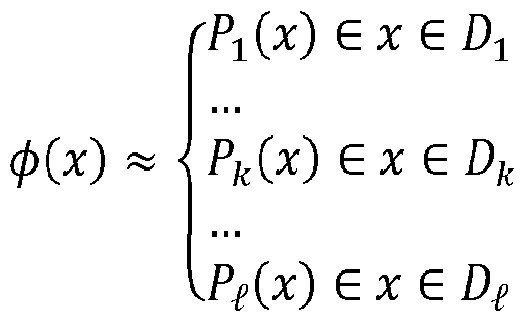
  • the optimization problem (7) is solved for a range of operating points for the motor offline to generate a set of data points, which are then mapped to a piecewise function (e.g., piecewise affine, piecewise quadratic, piecewise cubic) with domains divided by, for example, motor speed ( ⁇ ), to approximate the optimization problem (7).
  • a piecewise function e.g., piecewise affine, piecewise quadratic, piecewise cubic
  • the piecewise function is stored in the motor controller 120 and executed (i.e., solved) in real-time (online) based on input parameters (e.g., torque reference (T*) and motor speed ( ⁇ )). Additional discussion for generating such piecewise functions, including examples using surface reconstruction techniques and/or mesh reduction techniques, is provided below.
  • input parameters e.g., torque reference (T*) and motor speed ( ⁇ )
  • T* torque reference
  • motor speed
  • OERG -24- Q B ⁇ 175073.00216 ⁇ 90201874.3 Attorney Docket No.: 175073.00216 control scheme uses constraints, limiting the function to the explicit parameters and limiting the problem to their feasible sets, which implies that voltages, currents, fluxes, and the relationships between them are well behaved, or well-formed.
  • Experimental Results for OERG [0093] Experimental results for the OERG-based reference generation technique described above with respect to an example of the OERG block 215 (FIG. 2) and block 310 (FIG. 3) are provided below. FEA data for a 65kW WRSM with parameters shown in Table 1 are used to calculate the loss coefficients.
  • Table 1 WRSM Parameters Parameter Value Pole pairs ⁇ 2 Nameplate r-axis inductance ⁇ ⁇ 1.956 mH Nameplate d-axis inductance ⁇ ⁇ 2.420 mH N ameplate q-axis inductance ⁇ ⁇ 0.789 mH Base speed 30001/min Max speed 120001/min DC-link voltage 325 V Maximum power 65 kW Maximum torque 220 Nm [0094]
  • ⁇ and ⁇ were computed by using the least squares approach, e.g., for ⁇ , ⁇ ⁇ ⁇ ⁇ ⁇ ⁇ ⁇ ⁇ ⁇
  • similarly for ⁇ , ⁇ ⁇ ⁇ ⁇ ⁇ ⁇ ⁇
  • the matrices are -25- Q B ⁇ 175073.00216 ⁇ 90201874.3 Attorney Docket No.: 175073.00216 5 .6 0.0 0.0 0.0 0.0 0.0 0.0 ⁇ ⁇ ⁇ 0.0 0.045 0.0 ⁇ , ⁇ ⁇ ⁇ 0.0 0.0033 0.0 0 .0 0.0 0.045, 0.0 0.0 [0095]
  • the optimization problem (7) can be solved using a solver such as, for example, Matlab’s fmincon over the full operating of range of torques ⁇ ⁇ ⁇ that are within bounds of ( ⁇ ⁇ I) and ( ⁇ ⁇ ⁇ ) via (1) and the field weakening is enforced by the equation (8).
  • the static outputs are local or globally optimal operating points of the machine.
  • Optimal Efficiency Reference Generation Function with Multiple Affine Models
  • producing optimal reference currents that minimize copper loss and core loss for a combination of torque and speed is generally a difficult problem to solve analytically given the many non-linearities in a machine, but can be necessary for efficient operation of a machine.
  • traditional methods of mapping a motor, or non-linear power converter system, in a computationally efficient manner is limited – particularly in a highly dimensional space. For example, the magnetic behavior of a wound rotor synchronous (WRS) machine changes between zero torque and rated torque.
  • RFS wound rotor synchronous
  • a machine at zero torque, a machine may have a saliency ⁇ ⁇ ⁇ ⁇ ⁇ ⁇ ⁇ ⁇ , and at rated torque, the WRS machine may have a saliency ⁇ ⁇ ⁇ ⁇ ⁇ ⁇ ⁇ .
  • This variation in behavior may result from the phenomena of magnetic saturation in the WRS machine.
  • an affine magnetics model is created at each of these and an optimization problem for reference generation may be solved at each of these two points. The solution sets may ultimately be used to control the WRS machine.
  • an affine magnetics model is created at more than two points, the optimization problem for reference -26- Q B ⁇ 175073.00216 ⁇ 90201874.3 Attorney Docket No.: 175073.00216 generation is solved at each of these points, and resulting solution sets may ultimately be used to control the WRS machine.
  • the dq-axis stator current of the WRS machine (using the power-invariant Clarke-Park transform) may be limited by a stator rated current ⁇ ⁇ , ⁇ , while the rotor axis current is limited by a rated rotor current ⁇ ⁇ , ⁇ . These limits may be set by thermal constraints.
  • the current set I is thus constrained by a cylindrical shape (shown in FIG.7A).
  • inductances may be represented as a matrix ⁇ ⁇ R ⁇ and flux offsets may be expressed as ⁇ ⁇ R as in (9*).
  • V ⁇ ⁇ ariables ⁇ ⁇ and ⁇ ⁇ refer inductances, which are the diagonal terms of these inductance matrices.
  • the torque set ⁇ ⁇ is ⁇ ⁇ ⁇ ⁇ ⁇ ⁇ ⁇ ⁇ ⁇ R
  • the negative with the positive can achieve ⁇ ⁇ ⁇ , ⁇ ).
  • the magnitude of the stator voltage ( ⁇ ⁇ ⁇ ⁇ ) in the ⁇ ⁇ or dq reference frame for synchronous machines is bounded by ⁇ ⁇ ⁇ ⁇ ⁇ /2 or ⁇ ⁇ ⁇ ⁇ ⁇ / ⁇ 3 (if third harmonic injection is used) in a hexagonal shape.
  • the base speed of the machine ⁇ ⁇ is defined as when the product of the stator flux and electrical speed reaches the max stator voltage, or -28- Q B ⁇ 175073.00216 ⁇ 90201874.3 Attorney Docket No.: 175073.00216 [00107] Beyond base speed ⁇ ⁇ the stator flux is decreased (flux weakening) below ⁇ ⁇ , ⁇ while at maximum voltage, allowing for higher speeds, at the cost of decreased torque by (1) of the previous section.
  • the maximum speed of the WRS motor, ⁇ ⁇ may be set by mechanical limits.
  • FIG. 7A shows the torque speed-domain for one quadrant, including flux weakening.
  • a torque (except zero torque and maximum torque) produced by (1) has a non-unique set of currents and fluxes that can produce it. Given a reference (or feedback) torque and reference (or feedback) speed (depending on if using a torque or speed controller), producing the set of currents and fluxes that minimize the electrical losses in the machine can provide for optimal efficiency control.
  • the optimization problem (7) of the previous section may be used. However, in some examples, the optimization problem is modified to not include the constraint (8), but may still use the other constraints (9)-(11). In either case, the optimization problem (7) is solved two separate times for each of the two affine current to flux approximations in (7*) and (8*), once where constraint (9) is ⁇ ⁇ ⁇ ⁇ and once where constraint (9) is ⁇ ⁇ ⁇ ⁇ .
  • the torque equation (1) in constraint (10) is fixed to a reference torque, and constraint (11) fixes the speed to a constant.
  • the optimization problem (cost function) (7) is quadratic and the constraints are all affine except the torque constraint (10), which is quadratic and not convex. For this reason, additional considerations can be included when solving to help the numerical solver to reach a feasible solution.
  • An additional parameter ⁇ can be added to (11), which is minimized, or ⁇ ⁇ ⁇ ⁇ , ⁇ ⁇ ⁇ ⁇ ⁇ ⁇ ⁇ , and both ⁇ ⁇ and ⁇ can be minimized.
  • the current constraint I can be modified to have a strictly positive rotor current, i.e., ⁇ ⁇ ⁇ 0, in this way the solver will avoid symmetric guess ⁇ ⁇ ⁇ , ⁇ ⁇ ⁇ which can be chosen based on predicted efficient points, or based on previous optimization iterations can be loaded into the solver.
  • the motor controller 120 e.g., the processor 125
  • the motor controller 120 is operable to solve the optimization problem (7) for control in real time, like described in the previous OERG section.
  • the motor controller 120 may determine which of the affine models to utilize (e.g., at each operation point when a reference is to be generated). For example, the motor controller 120 may detect a motor characteristic of the motor during operation (e.g., motor current or motor torque) and then select the affine model to use to generate the reference based on the motor characteristic.
  • the motor characteristic may correlate to magnetic saturation of the motor.
  • the motor controller 120 may solve the optimization problem (7) where the constraint (9) is ⁇ ⁇ ⁇ ⁇ (corresponding to the first affine model).
  • the motor controller 120 may solve the optimization problem (7) where the constraint (9) is ⁇ ⁇ ⁇ ⁇ (corresponding ot the second affine model).
  • the motor controller 120 may implement an online, real-time solver.
  • the real-time solver may be a constrained gradient solver, primal dual interior point solver, or a numerical solver, or the like.
  • the motor controller 120 e.g., via block 215) -30- Q B ⁇ 175073.00216 ⁇ 90201874.3 Attorney Docket No.: 175073.00216 solves the optimization problem (7) with the selected constraint in real time by accessing a map or lookup table corresponding to the optimization problem (7) with the selected constraint generated in advance offline and stored in a memory (e.g., the memory 130).
  • the optimization problem (7) is solved for a range of operating points for the motor offline to generate a set of data points, which are then mapped to a respective piecewise function (e.g., piecewise affine, piecewise quadratic, piecewise cubic) with domains divided by, for example, motor speed ( ⁇ ), to approximate the optimization problem (7).
  • a respective piecewise function e.g., piecewise affine, piecewise quadratic, piecewise cubic
  • motor speed
  • each piecewise function corresponds to one of the affine models (e.g., a first piecewise function corresponding to the first affine model and a second piecewise function corresponds to the second affine model).
  • the piecewise functions are stored in the motor controller 120 and, during operation of the motor, one is selected (e.g., based on saturation as indicated by current or torque relative to a threshold.
  • the motor controller 120 may execute (i.e., solve) in real-time (online) the selected piecewise function based on input parameters (e.g., torque reference (T*) and motor speed ( ⁇ )). Additional discussion for generating such piecewise functions, including examples using surface reconstruction techniques and/or mesh reduction techniques, is provided below. [00114] In some examples, the optimization problem (7) is solved in real time for each constraint (e.g., solved with ⁇ ⁇ ⁇ ⁇ and also solved with ⁇ ⁇ ⁇ ⁇ ), and the motor controller 120 selected to affine model to use in reference by selecting the particular solution corresponding to the selected affine model to use for the reference generation.
  • T* torque reference
  • motor speed
  • the motor controller 120 may select the solution to use based on the saturation of the motor, which may be indicated by motor current or torque (e.g., being above or below a threshold), as described above.
  • This section describes use of two affine models, each corresponding to a motor saturation level as indicated by motor current or motor torque, that the motor controller 120 selects between to generate a reference.
  • more than two affine models are used, where each affine model corresponds to a magnetic saturation level (e.g., as indicated and defined by a motor current or motor torque range).
  • the motor controller 120 may select a first affine model when motor current (or torque) is between 0 and a first threshold, may select a second affine model when motor current (or torque) is between the first threshold and a second (higher) threshold, and may select a third affine model when the motor current (or torque) is above the second threshold.
  • a -31- Q B ⁇ 175073.00216 ⁇ 90201874.3 Attorney Docket No.: 175073.00216 corresponding threshold may be included such that each affine model corresponds to a magnetic saturation level range (e.g., as defined by a range of current or torque values).
  • the variables ⁇ and ⁇ are computed by using a least squares approach, e.g., where, for ⁇ , ⁇ ⁇ ⁇ ⁇ ⁇ ⁇ ⁇ ⁇ ⁇ ⁇
  • An FEA dataset sweeps the parameters ⁇ , ⁇ , ⁇ , ⁇ , and outputs ⁇ ⁇ , ⁇ ⁇ , ⁇ ⁇ .
  • the matrices are 0 .004 0.0 0.0 ⁇ ⁇ ⁇ , ⁇ .
  • Table 2 WRS Motor Drive Parameters Parameter Value Turns ratio ⁇ ⁇ / ⁇ ⁇ 39 Pole pairs ⁇ 2 Stator resistance ⁇ ⁇ 11.732 m ⁇ Rotor resistance (stator referred) ⁇ ⁇ 5.461 m ⁇ Shaft inertia 22.76E-3 kg m ⁇ Switching frequency 10 kHz Sampling frequency 20 kHz Nameplate r-axis inductance ⁇ ⁇ 1.956 mH -32- Q B ⁇ 175073.00216 ⁇ 90201874.3 Attorney Docket No.: 175073.00216 N ameplate d-axis inductance ⁇ 2.420 mH Nameplate q-axis inductance ⁇ ⁇ 0.789 mH Base speed 30001/min Max speed 120001/min DC-link voltage 325 V Maximum power 65 kW Maximum torque 220 Nm [00118] Additionally, some operating points of interest for the WRS motor at zero torque and peak torque are provided below in Table 3.
  • the inductance matrices may be 2 .07 2.12 0.0 0.19 0.19 0.0 ⁇ ⁇ ⁇ 2.07 2.42 0.0 ⁇ , ⁇ ⁇ ⁇ ⁇ 0.18 0.28 0.0 ⁇ . 0 .0 0.0 0.79 0.0 0.0 0.31 -33- Q B ⁇ 175073.00216 ⁇ 90201874.3 Attorney Docket No.: 175073.00216 [00120]
  • the error is 278 Vs or 94% for d-axis flux and 101 Vs or 80% for q-axis flux.
  • the optimization problem (7) is solved twice using Matlab’s fmincon over the full operating of range of torques ⁇ ⁇ ⁇ that are within bounds of ( ⁇ ⁇ I) via (1) and the field weakening is enforced by (9).
  • the static outputs are local or globally optimal operating points of the machine.
  • the solution set using the zero torque approximation ⁇ ⁇ ⁇ ⁇ function is shown in FIG. 7C. At low speed, the trajectories generally follow a straight path of positive ⁇ ⁇ , ⁇ ⁇ , ⁇ ⁇ ; then, at higher speeds, the machine field weakens and d-axis current decreases.
  • OERG-based control as described herein, generates reference values that provide efficient motor operation, with more accurate estimations of non- linear losses (e.g., core losses) or general machine behavior, while considering saturation, with less data and computations, and that the OERG-based control is able to be implemented by a motor controller (e.g., microcontroller) in real time.
  • a motor controller e.g., microcontroller
  • These core loss estimation techniques may be used as the core loss term ⁇ ⁇ ⁇ ⁇ , ⁇ in the OERG optimization problem (7) to generate the target motor control parameter value.
  • the two models use just 15 and 12 floating point operations each, and use 9 or 729 coefficients each.
  • the analytical models have been validated through FEA simulation for a wound rotor synchronous machine (WRSM).
  • the core loss estimation methods have 12% and 53% average error over all operating points of the machine. Additionally, these methods are extremely light computationally and use very few coefficients, making them well-suited for real-time controllers for various applications, including in the OERG block 215 of the motor controller 120 (FIG. 2).
  • Example use-cases of the two models include maximum efficiency point selection, use in real- time control, and FEA outlier detection.
  • the current in a three-phase WRSM has two parts, the AC stator current ⁇ ⁇ which utilizes the dq-axis from the power-invariant Clarke-Park transform, and DC rotor (sometimes called field) current ⁇ ⁇ . The rotor is aligned to the stator d-axis.
  • the torque per pole pair of the machine is defined ⁇ :R ⁇ ⁇ R ⁇ ⁇ ⁇ ⁇ ⁇ ⁇ where ⁇ is the stator cross product matrix 0 0 0 and ⁇ is the number of pole pairs of [00128]
  • the maximum torque ⁇ ⁇ and speed ⁇ ⁇ are generally limited by mechanical constraints.
  • the rotor and stator can be “flux weakened" in the sense of a PMSM such that electrically there is one maximum torque (at ⁇ ⁇ , ⁇ and ⁇ ⁇ , ⁇ ) and a theoretically unlimited electrical speed.
  • Core loss also referred to as iron loss, or ⁇ ⁇ [W]
  • ⁇ ⁇ [W] Core loss
  • ⁇ ⁇ [W] Core loss
  • ⁇ ⁇ [W] Core loss
  • ⁇ ⁇ [W] Core loss
  • ⁇ ⁇ [W] Core loss
  • ⁇ ⁇ [W] Core loss
  • ⁇ ⁇ [W] Core loss
  • ⁇ ⁇ [W] Core loss
  • ⁇ ⁇ [W] may be modelled using the Steinmetz Equation, which in its simplest form is ⁇ ⁇ ⁇ ⁇ ⁇ ⁇ ⁇ ⁇ ⁇ (19) where ⁇ is a coefficient, ⁇ ⁇ is the switching frequency, and ⁇ ⁇ is the peak value of the magnetic flux density.
  • the machine speed is the rate at which the magnetic flux of the core material changes, so ⁇ replaces ⁇ ⁇ .
  • Flux density ⁇ ⁇ is proportional to the more commonly used machine flux ⁇ , which leads to the equation ⁇ ⁇ ⁇ ⁇ ⁇
  • equation (20) [00130] While this equation may be too general to apply to a real-world system, a choice of exponents ⁇ and ⁇ can be chosen using some estimations to the underlying physics of the machine. There are many variations of equation (20)) used in motor loss modelling.
  • One example, called the Bertoti iron loss formula uses terms representing hysteric loss, lamination thickness, and excess loss with coefficients ⁇ ⁇ , ⁇ of ⁇ 2,1 ⁇ , ⁇ 2,2 ⁇ , ⁇ 1.5,1.5 ⁇ as ⁇ ⁇ ⁇ ⁇ ⁇ ⁇ ⁇ ⁇ ⁇ ⁇ ⁇ ⁇ ⁇ ⁇ ⁇ ⁇ . ⁇ ⁇ . ⁇ . ⁇ . ⁇ .
  • the first core loss model is ⁇ ⁇ ⁇ ⁇ ⁇ ⁇ ⁇ ⁇ ⁇ ⁇ , (22) and, when considering ⁇ is a ⁇ 3 ⁇ 1 ⁇ matrix from (16), becomes ⁇ ⁇ , ⁇ ⁇ ⁇ ⁇ ⁇ ⁇ ⁇ ⁇ (23) Where the coefficient ⁇ is distributed ⁇ term of flux ⁇ is simple to compute. A linear term ⁇ ⁇ 1 could potentially be added.
  • This model can be called the global model, or ⁇ ⁇ , ⁇ . Torque and speed both contribute to this ⁇ ⁇ equation, with speed proportional to the ⁇ ⁇ term and torque as part of the flux term ⁇ in equation (17).
  • FIG.9A illustrates a trend of the global model against torque, speed, and flux.
  • the second core loss model is ⁇ ⁇ ⁇ ⁇ ⁇ ⁇ ⁇ ⁇ ⁇ ⁇ ⁇ ⁇ ⁇ ⁇ ⁇ ⁇ ⁇ ⁇ ⁇ ⁇ ⁇ ⁇ ⁇ ⁇ ⁇ ⁇ ⁇ ⁇ ⁇ ⁇ ⁇ ⁇ for a set of discrete there is a separate ⁇ ⁇ matrix per discrete speed.
  • This core loss model is binned by speed, and thus denoted ⁇ ⁇ , ⁇ .
  • the second core loss model may also be represented as: ⁇ ⁇ ⁇ ⁇ ⁇ ⁇ ⁇ ⁇ ⁇ ⁇ ⁇ ⁇ ⁇ ⁇ ⁇ ⁇ ⁇ ⁇ ⁇ , ⁇ ⁇ , ⁇ ⁇ ⁇ ⁇ , ⁇ ⁇ ⁇ ⁇ ⁇ , ⁇ ⁇ ⁇ ⁇ ⁇ ⁇ ⁇ ⁇ ⁇ , ⁇ ⁇ ⁇ ⁇ ⁇ ⁇ ⁇ ⁇ ⁇ , ⁇ ⁇ ⁇ ⁇ ⁇ ⁇ ⁇ ⁇ ⁇ ⁇ ⁇ , ⁇ ⁇ ⁇ ⁇ cover the -37- Q B ⁇ 175073.00216 ⁇ 90201874.3 Attorney Docket No.: 175073.00216 machine speeds ⁇ ⁇ ⁇ ⁇ ⁇ ⁇ ⁇ ⁇ ... ⁇ ⁇ ⁇ .
  • the model has n piecewise quadratic equations which each have three matrices of coefficients corresponding to the quadratic dependence on speed ( ⁇ ⁇ ), linear dependence on speed ( ⁇ ⁇ ), and no dependence on speed ( ⁇ ⁇ ), and can be formulated to be continuous.
  • This core loss model is also binned by speed.
  • the matrix ⁇ may be obtained by first having a set of available loss datapoints ⁇ ⁇ ⁇ , ⁇ , ⁇ and solving the following convex optimization problem using all points ⁇ ⁇ ⁇ ⁇ ⁇ ⁇ ⁇ ⁇ ⁇
  • the two core loss models were run on a 65 kW WRSM with parameters shown in TABLE 4, where any such parameter could also be considered a feasible dimension in certain embodiments.
  • the FEA dataset used had 498,606 FEA datapoints ⁇ ⁇ ⁇ , ⁇ , ⁇ corresponding to the full current range of the machine ⁇ ⁇ ⁇ I and 81 specific speeds ⁇ ⁇ .
  • the values for ⁇ were negligible for all terms except ⁇ ⁇ , ⁇ and ⁇ ⁇ , ⁇ which are the self-induced stator core losses of the d-axis and q-axis respectively. This is because for this specific WRSM, the rotor is excited by DC current.
  • the values are shown in TABLE 5 and FIGS.8B-C.
  • core loss error for the global model is shown in the upper plots of FIG.10, and core loss error for the binned model is shown in the lower plots of FIG.10.
  • Boxplots showing the error of both core loss models are shown in FIG. 11A, and average core loss error between FEA and the global and binned analytics models are shown according to speed in FIG. 11B.
  • the error tends to decrease dramatically for both models as speed is increased.
  • the average error for ⁇ ⁇ , ⁇ is 12% compared to an average error of 53% for ⁇ ⁇ , ⁇ .
  • ⁇ ⁇ , ⁇ is much more accurate, but considerably slower than ⁇ ⁇ , ⁇ . It is likely that not all 81 speeds in the piecewise function are necessary to have a reasonably accurate core loss model. Accordingly, in some examples, the piecewise function has fewer than 81 speeds (i.e., fewer bins) and, thus, fewer than 81x more coefficients.
  • Example benefits of these two core loss models versus more complex models are 1) increased speed of computation 2) relatively low error 3) no need to know complex machine geometry, and 4) includes core losses from coupled flux. These benefits allow for a wide range of potential applications including fast maximum efficiency point selection, use a cost in a real- time controller when moving between reference speed-torques, and FEA outlier detection.
  • the state space model of the system uses the flux ⁇ ⁇ ⁇ R ⁇ in the stator dq-axis (using the magnitude-invariant Clarke-Park transform) and rotor axis (aligned to the d-axis) as the state variable ⁇ ⁇ ⁇ ⁇ ⁇ ⁇ ⁇ ⁇ ⁇ ⁇ ⁇ , (30) ⁇ ⁇ ⁇ ⁇ ⁇ ⁇ ⁇ ⁇ ⁇ ⁇ ⁇ ⁇ ⁇ ⁇ , (31) ⁇ ⁇ ⁇ ⁇ [00147]
  • the inputs are a the stator and rotor voltages ⁇ ⁇ .
  • ⁇ ⁇ R is the mechanical speed (1/min) multiplied by ⁇ ⁇ ⁇ ⁇ , where ⁇ is the number of pole pairs of the machine.
  • -42- Q B ⁇ 175073.00216 ⁇ 90201874.3 Attorney Docket No.: 175073.00216 [00148]
  • the relationship between the current ⁇ ⁇ ⁇ R ⁇ and flux ⁇ ⁇ is nonlinear, and has saturation and cross saturation effects. This can be modelled by the continuous nonlinear function ⁇ ⁇ , , and the inverse can be modelled by ⁇ ⁇ ⁇ ⁇ ⁇ ⁇ ⁇ .
  • the maximum value of the torque function is dependent on speed by m ax ⁇ ⁇ ⁇ ⁇ ⁇ ⁇ ⁇ / ⁇ , ⁇ ⁇ ⁇ ⁇ ⁇ . (43) Q B ⁇ 175073.00216 ⁇ 90201874.3 Attorney Docket No.: 175073.00216 [00154]
  • the domain (inputs) of optimal generation map are speeds and torques bounded by (43), the range (output) is a set of currents ⁇ ⁇ that may be requested (e.g., of the controller 240).
  • the largest sources of electrical losses in a machine are copper loss ⁇ ⁇ ⁇ ⁇ , ⁇ , ⁇ R ⁇ ⁇ R ⁇ and iron loss ⁇ ⁇ ⁇ ⁇ , ⁇ , ⁇ R ⁇ ⁇ R ⁇ .
  • Copper loss has a typically square dependence on current and linear by resistance.
  • the resistance of the stator and rotor vary non- linearly with machine temperature and speed, and are also frequency dependent.
  • the core loss is even more difficult to model with an analytical function, it typically has a square dependence on flux ⁇ (which is nonlinearly dependent on current) and speed ⁇ .
  • the two largest sources of core loss are eddy currents and hysteresis, which are both difficult to model.
  • problem (45) can be solved for all combinations of (43).
  • the solution set for all torque and speed combinations can be assigned to a continuous function ⁇ ⁇ ⁇ ⁇ ⁇ ⁇ ⁇ ⁇ , ⁇ ⁇ ⁇ R ⁇ ⁇ R ⁇ . Because there is no equation for the objective function, there is also no analytical solution.
  • a pareto frontier can be constructed using the points in ⁇ ⁇ ⁇ which minimizes electrical loss ⁇ ⁇ ⁇ ⁇ , ⁇ , ⁇ .
  • Pareto frontiers are a collection of pareto optimal points from a set of discrete datapoints that minimize one dimension of the objective function.
  • the pareto optimal FEA datapoints are denoted ⁇ ⁇ , and ⁇ ⁇ ⁇ ⁇ .
  • ⁇ ⁇ is the discretized FEA solution to (45).
  • the discrete pareto-optimal points ⁇ ⁇ may be used to create a continuous pareto- optimal surface ⁇ ⁇ ⁇ (simplical mesh) that best approximates the ideal surface ⁇ ⁇ .
  • a surface reconstruction technique may be used to translate the discrete pareto-optimal points ⁇ ⁇ to a continuous pareto-optimal surface ⁇ ⁇ ⁇ .
  • Such a surface reconstruction technique may depend on the original surface, ⁇ ⁇ , being a surface (two-dimensional manifold) that is compact, connected, and orientable.
  • a surface reconstruction technique such as described in “Surface Reconstruction from Unorganized Points” (Hoppe et al. 1992), takes as input an organized set of points on or near an unknown manifold M and produces as output a simplicial surface that approximates M.
  • the surface reconstruction technique that is employed includes a first stage to define a function f that estimates the signed geometric distance to the unknown surface M, and a -45- Q B ⁇ 175073.00216 ⁇ 90201874.3 Attorney Docket No.: 175073.00216 second stage that uses a contouring algorithm to approximate Z(f) by a simplical surface, where zero set Z(f) is an estimate for M.
  • an oriented plane may be associated with each of the data points.
  • Each plane (referred to as tangent planes) may serve as a local linear approximation to the surface.
  • the tangent planes may not directly define the surface because their union may have a complicated non-manifold structure.
  • the tangent planes may define the signed distance function to the surface.
  • other surface reconstruction techniques may be employed.
  • the FEA method will produce a set of discrete points ⁇ ⁇ ⁇ ⁇ which will have some sampling density ⁇ and noise factor ⁇ .
  • a sampled space is said to be ⁇ ⁇ dense if for any sphere with radius ⁇ ⁇ R ⁇ there is at least one sample point ⁇ . If the original sample ⁇ has some ⁇ ⁇ density, then the pareto points ⁇ ⁇ will have a ⁇ ⁇ density less than or equal to the original ⁇ ⁇ density, as ⁇ ⁇ ⁇ .
  • ⁇ ⁇ ⁇ density in ⁇ it may be necessary to have a higher ⁇ ⁇ density than in ⁇ , requiring denser sampling in the FEA.
  • Any pareto point ⁇ ⁇ , ⁇ will be equal to the ideal surface with some added error, or ⁇ , ⁇ ⁇ ⁇ ⁇ ⁇ ⁇ ⁇ .
  • a sampled space is called ⁇ ⁇ noisy if
  • the ⁇ value (or maximum error) for an FEA simulation is generally known, and decreases with the size of the simplical mesh.
  • the discrete points produced by the FEA method will serve as an input to the surface reconstruction technique to generate the be used to translate the discrete pareto-optimal points ⁇ ⁇ to a continuous pareto-optimal surface ⁇ ⁇ ⁇ , which is a simplical mesh.
  • an optimization problem is employed (e.g., in OERG block 215 of FIG.2 and/or in block 310 of FIG.3) that does not consider core losses and, rather, focuses on minimizing copper losses. Such an optimization problem may provide a less complex function while still providing efficient motor operation.
  • the process 300 of FIG.3 and operation of the system 200 may otherwise proceed similarly to the other examples discussed herein.
  • the following optimization problem may minimize copper losses given any torque and any speed that satisfies equation (43): ⁇ ⁇ ⁇ ⁇ min ⁇ , ⁇ ⁇ ⁇ ⁇ ⁇ , ⁇ , ⁇ (51) ⁇ ⁇ ⁇ ⁇ .
  • FEA method may be employed to approximate loss using this copper loss-focused optimization problem.
  • the FEA method locally linearizes nonlinear thermal and magnetic equations using simplical meshes given a set of inputs.
  • An example may be inputs of fixed current ⁇ ⁇ I and speed ⁇ ⁇ ⁇ , and outputs may be copper loss ⁇ ⁇ , resistance R, and flux ⁇ .
  • Pareto frontiers are a collection of pareto optimal points from a set of discrete datapoints that minimize one dimension of the objective function[42].
  • the pareto optimal FEA datapoints are denoted ⁇ ⁇ , and ⁇ ⁇ ⁇ ⁇ .
  • ⁇ ⁇ is the discretized FEA solution to (51).
  • a simplical complex in R ⁇ can be constructed using the points ⁇ ⁇ and a triangulation algorithm such as the Delaunay triangulation.
  • the simplical complex is denoted ⁇ ⁇ ⁇ . [00171] Regardless of whether using the optimization problem of (7), (45) or (51), the FEA method may be applied to provide discrete pareto-optimal points ⁇ ⁇ that may be translated into a simplical complex ⁇ ⁇ ⁇ .
  • a surface reconstruction technique may be employed to generate the simplical complex denoted ⁇ ⁇ ⁇
  • Delaunay triangulation may be employed to generate the simplical complex denoted ⁇ ⁇ ⁇
  • another decomposition technique may be employed to generate the simplical complex denoted ⁇ ⁇ ⁇ .
  • Delaunay triangulation is a known mathematical meshing algorithm or technique, and quad tree, box tree, KD-tree, and alpha shape are also known domain decomposition algorithms or techniques.
  • a Voronoi diagram of the current points may be constructed.
  • the Voronoi -47- Q B ⁇ 175073.00216 ⁇ 90201874.3 Attorney Docket No.: 175073.00216 diagram splits the current space into N Voronoi cells, where all points in a Voronoi cell are closer to a single point of the original set of current points than any other point.
  • the Delaunay triangulation one may find the dual of the Voronoi diagram.
  • the Delaunay triangulation maximizes the minimum angle in the simplices it creates, thus reducing “skinny” simplices.
  • “skinny” simplices may be described by their aspect ratio. In other words, a simplex having an aspect ratio above a threshold amount may be considered “skinny,” while a simplex having an aspect ratio below the threshold amount may be considered “not skinny.” [00173] For the resulting current simplices generated, each simplex is connected at a shared boundary to another simplex so that all simplices are connected within the domain, and no simplex overlaps another simplex within the domain. Additionally, the simplices may be defined such that they are closed domains on one side and open domains on the other such that any arbitrary point in the domain will belong to one and only one simplex within the Delaunay construction (even if the point is on a boundary).
  • the resulting simplical complex ⁇ ⁇ ⁇ may be a collection or mesh of simplices (e.g., of two-dimensional simplices in three-dimensional space).
  • a piecewise map or function may be fitted to the resulting simplical complex ⁇ ⁇ ⁇ , where the function may then be used to approximate the solution set.
  • the surface reconstructed as described above may be a collection of simplices in R ⁇ ⁇ ⁇ ⁇ ⁇ ⁇ ⁇ , ⁇ ⁇ ⁇ ⁇ ⁇ , ⁇ 1/ ⁇ ⁇ ⁇ space.
  • the optimal output current set ⁇ ⁇ is generated by using a piecewise affine function defined by the vertices of ⁇ ⁇ ⁇ .
  • Each simplex will have an affine equation assigned to it such that the overall function will be closed and continuous.
  • Each simplex (plane) in ⁇ ⁇ ⁇ is defined as the convex hull of three of three points ⁇ , ⁇ ⁇ H ⁇ ⁇ ⁇ ⁇ ⁇ , ⁇ , ⁇ ⁇ ⁇ , ⁇ ⁇ ⁇ , ⁇ ⁇ ⁇ .
  • FIG. 14B shows pareto-optimal datapoints ⁇ ⁇ with iso- power curves
  • FIG.14C shows pareto-optimal surface ⁇ ⁇ ⁇ .
  • FIG.14D illustrates electrical losses from experimental testing with a machine controlled according an example simplical complex formed using surface reconstruction. In this testing, the machine is controlled with a 120 second drive cycle with positive and negative torques, where the machine includes -49- Q B ⁇ 175073.00216 ⁇ 90201874.3 Attorney Docket No.: 175073.00216 parameters as shown in Table 4 above. The current from h ⁇ ⁇ is mapped back to torque to show the difference in torque to the original requested torque.
  • Piecewise Maps [00181] As noted above, in some examples, the OERG-based motor control described herein uses a piecewise map (also referred to as a piecewise function).
  • a piecewise map may be a function that is fitted to a solution set of data points, where the function may then be used to approximate the solution set.
  • Piecewise maps divide a nonlinear map into M domains, where each of the M domains is made up of a (sub) function. In other words, sub-functions are pieces of the piecewise map and, collectively, form the piecewise map.
  • Piecewise maps may be classified as a piecewise constant map, piecewise affine map, piecewise quadratic map, piecewise cubic map, or a piecewise map with functions having an order higher than three.
  • the nonlinear map is divided into M domains over which the function may be constant values.
  • the nonlinear map is divided into M domains over which the function may be linearized.
  • the nonlinear map is divided into M domains over which the function may be quadratic.
  • the nonlinear map is divided into M domains over which the function may be cubic.
  • Piecewise maps of a higher order are similarly divided into M domains over which the function may be of the higher order. [00182] Piecewise maps divide the original domain into M domains or sets.
  • FIGS.12A-12B illustrate two piecewise maps. More particularly, FIG.12A illustrates a piecewise affine map (PWA map) and FIG. 12B illustrates a piecewise quadratic map (PWQ map).
  • Piecewise maps may be constructed with regularly or irregularly sampled points for data in any dimension, although there are some limitations for higher order polynomials.
  • to generate a piecewise map may include letting ⁇ ⁇ R ⁇ and ⁇ :R ⁇ ⁇ R be a potentially unknown C ⁇ function that is irregularly sampled m times subject to ⁇ ⁇ ⁇ -50- Q B ⁇ 175073.00216 ⁇ 90201874.3 Attorney Docket No.: 175073.00216 ... ⁇ ⁇ ⁇ ⁇ , with ⁇ ⁇ ⁇ ⁇ ⁇ ⁇ ... ⁇ and ⁇ ⁇ ⁇ ⁇ ⁇ ... ⁇ . Attention may be restricted to the convex hull ⁇ ⁇ ⁇ ⁇ hull ⁇ ⁇ ⁇ ⁇ R ⁇ .
  • the samples ⁇ may be triangulated into l simplices, for example, using the n-dimensional Delaunay method.
  • ⁇ ⁇ :l ⁇ ⁇ ⁇ ⁇ is connected, non-overlapping, and convex.
  • Each ⁇ is defined by ⁇ ⁇ 1 samples and ⁇ ⁇ hull ⁇ ⁇ ) with ⁇ ⁇ ⁇ ⁇ ⁇ , ... ⁇ ⁇ ⁇ .
  • piecewise multivariate polynomials ⁇ : ⁇ ⁇ R may be defined to approximate ⁇ .
  • piecewise multivariate polynomisals may be defined to approximate ⁇ as: ⁇ ⁇ ⁇ ⁇ ⁇ ⁇ ⁇ ⁇ ⁇ ⁇ ⁇ ⁇ [00185]
  • Example polynomials are form, in Table 7. Table 6 – Example Polynomials ⁇ of parameter Order Type Function Gradient Hessian ⁇ ⁇ 0 constant ⁇ ⁇ 0 0 1 1 affine ⁇ ⁇ ⁇ ⁇ ⁇ ⁇ 0 ⁇ ⁇ 1 2 quadratic ⁇ ⁇ ⁇ ⁇ ⁇ ⁇ ⁇ ⁇ ⁇ ⁇ ⁇ ⁇ ⁇ ⁇ ⁇ ⁇ ⁇ ⁇ ⁇ ⁇ ⁇ ⁇ ⁇ ⁇ ⁇ ⁇ ⁇ ⁇ ⁇ 1 cubic 3 ...
  • l ⁇ ⁇ ⁇ ⁇ will not leave any degrees of freedom to a fitting function. Therefore, it may be required that l ⁇ ⁇ . This can be useful for fitting to a low number of points and/or simplices.
  • An example relevant special case includes piecewise cubic functions (PWC).
  • piecewise fitting may include, where ⁇ are coordinates in ⁇ - dimensional space, ⁇ are the number of coordinates and values ⁇ ⁇ ⁇ , ⁇ ⁇ ⁇ , and l are the number of (Delaunay) simplices that triangulate the space, the following: ⁇ ⁇ vertices per simplex: ⁇ ⁇ ⁇ ⁇ ⁇ 1 ⁇ ⁇ parameters ⁇ per simplex of ⁇ ⁇ ⁇ ⁇ ⁇ ⁇ ⁇ ⁇ ⁇ ⁇ ⁇ ⁇ ⁇ ⁇ ⁇ ⁇ ⁇ ⁇ "Full ⁇ ⁇ ": ⁇ ⁇ ⁇ ⁇ ⁇ ⁇ 1 ⁇ ⁇ ⁇ ⁇ 1 ⁇ ⁇ 1 "sym ⁇ ⁇ ": ⁇ ⁇ ⁇ ⁇ ⁇ ⁇ ⁇ ⁇ 1 ⁇ ⁇ ⁇ values: ⁇ ⁇ ⁇ ⁇ ⁇ ⁇
  • Function value constraint ⁇ ⁇ ⁇ ⁇ ⁇
  • a data set of input operational points and corresponding output operational points is generated.
  • the data set may be generated through simulation (e.g., using finite element analysis (FEA)), through experimentation, or through a combination of simulation and experimentation.
  • FEA finite element analysis
  • a domain decomposition algorithm is applied to the data set to generate simplices.
  • Various domain decomposition algorithms or techniques also referred to as domain subdivision algorithms, may be applied to generate the simplices.
  • the domain decomposition algorithm or technique may be Delaunay triangulation or may be a surface reconstruction technique as described above.
  • the domain decomposition algorithm or technique may be an irregularly sampled, but rectangular, decomposition, for example, a quad tree algorithm, a box tree algorithm (also referred to as oct tree), or KD-tree algorithm (depending upon the number of independent dimensions).
  • the domain decomposition algorithm is an alpha shape algorithm or technique. For the resulting simplices generated, each simplex is connected at a shared boundary to another simplex so that all simplices are connected within the domain, and no simplex overlaps another simplex within the domain.
  • the simplices may be defined such that they are closed domains on one side and open domains on the other such that any arbitrary point in the domain will belong to one and only one simplex within the Delaunay construction (even if it is on a boundary). Examples of such connected simplices are shown in the PWA map of FIG.12A and the PWQ map of FIG.12B.
  • the binned core loss model (24) is implemented using a piecewise map.
  • the piecewise map is a piecewise quadratic (PWQ) map.
  • each of the M domains of the PWQ map corresponds to a motor speed range (e.g., ⁇ ⁇ ⁇ ⁇ ⁇ ⁇ ⁇ ⁇ ).
  • the motor controller 120 may select the M domain of the PWQ map (and, thus, the sub-function of the PWQ map) based on the motor speed of the motor 115. For example, when motor speed ( ⁇ ) is between ⁇ ⁇ and ⁇ ⁇ , the controller 120 will select and solve ⁇ ⁇ ⁇ ⁇ ⁇ ⁇ ⁇ to determine the core loss. This core loss may then be used in the reference generation by the OERG block 215 (e.g., when solving the optimization problem (7)).
  • the domains may be according to reference torque, motor speed, and additional parameters, such as, for example, current and/or voltage limit.
  • This technique in some examples, can be viewed as taking a system that has more than two degrees of freedom beyond torque and speed, and running an optimization to describe how best to collapse those additional degrees of freedom into torque and speed, so that the system operates withing its constraints.
  • the current-flux map (equation (9)) is implemented using a piecewise map, which may be a PWA map, PWC map, PWQ map, etc.
  • Using decomposition techniques, like Delaunay triangulation, to create a mesh over a multidimensional space e.g., dq0 or rdq0, for instance
  • a multidimensional space e.g., dq0 or rdq0, for instance
  • dq0 or rdq0 and speed, or rdq0, speed, and core losses, etc. the meshing becomes more challenging.
  • the mesh when relying strictly on the data to create the mesh, the mesh can become ill-formed or "not smooth.” Strictly relying on the data may refer to using FEA data to construct a motor model (e.g., describing the machine, which is used for the purposes of control). When operating a machine across a trajectory that crosses an ill-formed mesh, a proper response is not formulated. As a result, the ill-formed mesh affects control and motor dynamics because current may reverse, may jump from "peaks" to "valleys,” or the like, across this ill-formed (noisy) mesh.
  • constraints on the system that generate the meshes e.g., optimization problem (7)
  • constraints on the system that generate the meshes can create a much smoother surface, particularly when compared to a system relying only on the data (without such constraints) and/or without considering core losses to construct the mesh.
  • a trajectory -58- Q B ⁇ 175073.00216 ⁇ 90201874.3 Attorney Docket No.: 175073.00216 across the mesh (e.g., with piecewise functions) provides a more effective traversal.
  • a trajectory for example, identifies the most advantageous set point or operating points for the motor to produce certain torque and speed across a drive cycle or operating condition.
  • the motor controller 120 can consider multiple speeds and torques, and create a trajectory across flux and speed that operates the machine to accomplish that output at a high efficiency.
  • the PWA function may be generated using a separate computing device.
  • a computing device e.g., server, desktop, laptop, etc. having a memory and a processor, where the processor executes instructions retrieved from the memory to perform the various processing steps, algorithms, and techniques described above (e.g., FEA analysis, surface reconstruction, mesh reduction (described below), and the like) to generate the piecewise function.
  • the piecewise function may then be transmitted by the computing device (or another intermediary device) to the motor controller 120 for storage on the memory 130.
  • Mesh Reduction [00209]
  • a mesh reduction algorithm may be applied to the simplical complex.
  • each simplex corresponds to a domain or function of the piecewise function
  • the complexity and size of the ultimate piecewise function may be reduced.
  • less memory space may be used to store the piecewise function and a controller may execute the piecewise function (e.g., determine a target motor control parameter value based on a desired control parameter) more quickly.
  • the mesh reduction algorithm simplification is configured to maintain sufficient accuracy in its approximation of the optimization problem to remain effective and provide efficient reference generation.
  • the mesh reduction algorithm may be, for example, an edge contraction algorithm, a vertex contraction -59- Q B ⁇ 175073.00216 ⁇ 90201874.3 Attorney Docket No.: 175073.00216 algorithm, and/or a vertex decimation algorithm.
  • a vertex contraction algorithm may be based on an iterative contraction of vertex pairs where, to contract a vertex pair, the vertices of the pair are moved to a new position, the pair’s incident edges are connected to one vertex of the pair, the other vertex of the pair is deleted, and, subsequently, edges or faces that have become degenerate are removed.
  • the simplical complex (also called simplical mesh) ⁇ ⁇ ⁇ has a connected domain; that is, in the domain ( ⁇ ⁇ , ⁇ ), there are no gaps in the triangles.
  • a connected domain is generally guaranteed for the Delaunay triangulation method, but, not for all surface reconstruction methods.
  • the domain ( ⁇ ⁇ , ⁇ ) is bounded by (43), so the surface is open.
  • ⁇ ⁇ ⁇ is a connected, open two-dinemsional manifold.
  • Mesh reduction algorithms aim to reduce the number of simplices in a simplical complex while preserving the general shape. They are either topology preserving or non- topology preserving. Non-topology preserving algorithms may change the topological properties of the surface.
  • non-topology preserving algorithms include vertex contraction and vertex clustering.
  • vertex contraction and vertex clustering For the PWA map, it may be detrimental for the map to go from connected to unconnected, as the output reference currents would be undefined.
  • Two iterative approaches that mesh reduction algorithms may follow include: 1) setting the maximum number of simplices or 2) setting the maximum allowable error. Some algorithms work with both such as edge contraction, vertex contraction, and vertex decimation. The memory and time constraints may be directly dependent on the number of simplices ⁇ . Accordingly, in some examlpes, the first option is used to specify the maximum number of simplices. Some algorithms, for example, simplification envelopes, set a maximum Euclidean distance ⁇ between the original and reduced meshes and reduce until that distance is met.
  • Each simplex in the simplical complex ⁇ ⁇ ⁇ may have a set of three-dimensional affine coefficients (slope ⁇ ⁇ and intercept ⁇ ⁇ ) as per (60).
  • the input dimension ⁇ (dimension of ⁇ ) and output dimension ⁇ (dimension of ⁇ ) will produce a PWA function with a slope matrix sized ⁇ ⁇ ⁇ ⁇ and offset vector ⁇ ⁇ ⁇ 1 ⁇ .
  • the boundaries of each simplex are defined by the ⁇ ⁇ 1 affine equations defining the H-notation of the simplex ⁇ ⁇ ⁇ ⁇ .
  • the overall number of coefficients may be ⁇ ⁇ ⁇ ⁇ ⁇ ⁇ ⁇ 2 ⁇ ⁇ ⁇ 1 ⁇ ⁇ ⁇ ⁇ ⁇ 2 ⁇ ⁇ ⁇ ⁇ 2 ⁇ , or the number of -60- Q B ⁇ 175073.00216 ⁇ 90201874.3 Attorney Docket No.: 175073.00216 coefficients increases linearly with the number of simplices ⁇ ⁇ .
  • the simplical complex may be stored in a tree structure whereby the search time complexity is ⁇ ⁇ ⁇ ⁇ ⁇ ⁇ ⁇ without warm starting and ⁇ 1 ⁇ with warm starting. [00214] Given an allotted amount of memory on a microcontroller, the number of simplices ⁇ ⁇ that can fit in memory can be predicted.
  • the number of simplices ⁇ ⁇ that can be used without running out of time can be predicted.
  • the smaller of ⁇ ⁇ and ⁇ ⁇ may be selected and used as the target number of simplices.
  • certain mesh reduction algorithms are used for online level-of-detail (LOD) modelling, and are designed to perform quickly, but may sacrifice some accuracy.
  • the MTPA PWA map is computed offline and the static map is loaded onto a controller (e.g., the motor controller 120). In such examples, fast computation may be less of a priority.
  • the mesh reduction algorithm used is vertex contraction, which can change the topological properties of the mesh, but joins surfaces, rather than separate surfaces.
  • the resulting piecewise map corresponding to a simplical complex output or provided by application of the mesh reduction algorithm may be employed by the motor controller 120 to use or solve the optimization problem (e.g., (7), (45), or (51)) to determine the target motor control parameter values (e.g., as described with respect to block 310 of FIG. 3).
  • the piecewise function may be stored in the memory 130 of the motor controller 120 and, to execute OERG block 215 of FIG. 2 and/or block 310 of FIG.
  • the motor controller 120 solves the piecewise function with the desired control parameter (torque and/or speed) as an input to the piecewise function.
  • the output or solution of the piecewise function may be, for example, the reference current ir* or, when OERG block 215 is integrated with the flux linkage map block 220, the reference flux ⁇ r * (see, e.g., FIG.2).
  • FEA analysis on a 65kW WRSM was performed.
  • the copper loss datapoints and pareto-optimal points in ( ⁇ ⁇ , ⁇ , ⁇ ⁇ ) space are shown in FIGS. 14A and 14B, respectively.
  • An initial simplical complex was generated that includes 44,640 simplices (see FIG.
  • a vertex contraction mesh reduction algorithm was applied to the initial simplical complex to reduce the number simplices to 4,463 in a first iteration (see FIG. 15B), to 446 -61- Q B ⁇ 175073.00216 ⁇ 90201874.3 Attorney Docket No.: 175073.00216 simplices in a second iteration (see FIG.15C), and to 45 simplices in a third iteration (see FIG. 15D). Accordingly, after three mesh simplification steps (e.g., three iterations of mesh reduction via vertex contraction), the number of simplices was reduced by 1000x to generate a simplical complex of 45 faces (see FIG.15D).
  • the motor controller 120 in any of its various configurations described herein (see, e.g., FIG. 2) is implemented as a set of instructions stored on a nontransitory computer readable medium, where the instructions are for execution by a processor.
  • the processor may be configured to (or may be connected to another device configured to) simulate a motor, power supply, and power switching network (simulating an arrangement similar to, for example, the arrangement in FIG. 2).
  • the processor through execution of the set of instructions, may be configured to monitor and control a motor where the motor is a simulated motor coupled to a simulated power supply via a simulated power switching network.
  • Example 1 A method, apparatus, and non-transitory computer-readable medium for motor control comprises: a power switching network configured to be coupled to a power supply and to a motor; and an electronic controller configured to: determine current values for the motor in a rotational reference frame, each current value associated with a dimension of a set of dimensions of the rotational reference frame; determine, based on a desired control parameter, a target motor control parameter value for each dimension of the set of dimensions of the rotational reference frame using an optimization cost function that considers motor speed, copper -62- Q B ⁇ 175073.00216 ⁇ 90201874.3 Attorney Docket No.: 175073.00216 loss, and core loss; and control the power switching network based on the current values and the target motor control parameter values.
  • Example 2 The method, apparatus, and non-transitory computer-readable medium according to Example 1, wherein the optimization cost function considers core loss by using a global core loss model with a matrix G of coefficients applicable regardless of motor speed of the motor.
  • Example 3 The method, apparatus, and non-transitory computer-readable medium according to any of Examples 1 to 2, wherein the optimization cost function considers core loss by using a binned core loss model with a matrix of coefficients that depends on a speed of the motor.
  • Example 4 The method, apparatus, and non-transitory computer-readable medium according to any of Examples 1 to 3, wherein the optimization cost function considers core loss by using a binned core loss model, wherein the binned core loss model is implemented as a piecewise function with M domains defined by motor speed, each of the M domains corresponding to a motor speed range and a matrix G of coefficients.
  • Example 5 The method, apparatus, and non-transitory computer-readable medium according to any of Examples 1 to 4, wherein, a solution set of the optimization cost function is defined as a piecewise function with M domains, each of the M domains corresponding to a motor speed range and a motor torque range.
  • Example 6 The method, apparatus, and non-transitory computer-readable medium according to Example 5, wherein each of the M domains of the piecewise function corresponds to a simplex of a surface reconstructed from a set of pareto optimal points of datapoints derived from a set of inputs applied to the optimization cost function.
  • Example 7 The method, apparatus, and non-transitory computer-readable medium according to Example 5, wherein each of the M domains of the piecewise function corresponds to a simplex of a reduced simplical complex of a simplical complex, where simplical complex was formed from a set of pareto optimal points of datapoints derived from a set of inputs applied to the optimization cost function.
  • Example 8 The method, apparatus, and non-transitory computer-readable medium according to any of Examples 6 or 7, wherein the simplical complex was formed from the set of pareto optimal points using at least one selected from a group of a surface reconstruction technique and a triangulation technique.
  • Example 9 The method, apparatus, and non-transitory computer-readable medium according to Example 7, wherein the reduced simplical complex was formed using a mesh reduction technique to reduce the simplical complex to a target number of simplices.
  • Example 10 The method, apparatus, and non-transitory computer-readable medium according to any of Examples 5 to 9, wherein the piecewise function is stored in a memory of the electronic controller and, to determine the target motor control parameter value, the electronic controller solves the piecewise function with the desired control parameter as an input to the piecewise function.
  • Example 11 The method, apparatus, and non-transitory computer-readable medium according to any of Examples 1 or 10, wherein the optimization cost function is associated with a first model corresponding to a first magnetic saturation level of the motor and with a second model corresponding to a second magnetic saturation level of the motor, wherein a first solution set of the optimization cost function for the first model is defined as a first piecewise function with domains, each of the domains corresponding to a respective motor speed range and a respective motor torque range, wherein a second solution set of the optimization cost function for the second model is defined as a second piecewise function with further domains, each of the further domains corresponding to a respective motor speed range and a respective motor torque range, and wherein, to determine the target motor control parameter value using the optimization cost function, the electronic controller is configured to: select a piecewise function from the first piecewise function or the second piecewise function to use based on a motor characteristic of the motor during operation; and solve the piecewise function with the desired control parameter as an input to the piecewise function
  • Example 12 The method, apparatus, and non-transitory computer-readable medium according to any of Examples 1 or 11, wherein the optimization cost function is associated with a first model corresponding to a first magnetic saturation level of the motor and with a second model corresponding to a second magnetic saturation level of the motor, and wherein, to -64- Q B ⁇ 175073.00216 ⁇ 90201874.3 Attorney Docket No.: 175073.00216 determine the target motor control parameter value using the optimization cost function, the electronic controller is configured to: select a model from the first model or the second model to use based on a motor characteristic of the motor during operation; and use a solution of the model based on the desired control parameter as an input to the model.
  • Example 13 The method, apparatus, and non-transitory computer-readable medium according to any of Examples 1 or 12, wherein, to determine current values for the motor in a rotational reference frame, the electronic controller is configured to: determine electrical operational characteristics of the motor in a stationary reference frame; determine a rotational position of the motor; and transform the electrical operational characteristics and the rotational position to the current values for the motor in the rotational reference frame.
  • Example 14 The method, apparatus, and non-transitory computer-readable medium according to any of Examples 1 or 13, the electronic controller further configured to: determine, based on the current values, a flux linkage value for each dimension of the set of dimensions of the rotational reference frame, and wherein, to control the power switching network based on the current values, the electronic controller is configured to control the power switching network based on the flux linkage values determined from the current values.
  • Example 15 The method, apparatus, and non-transitory computer-readable medium according to any of Examples 1 or 14, wherein the desired control parameter is a target torque value for the motor.
  • Example 16 The method, apparatus, and non-transitory computer-readable medium according to any of Examples 1 or 15, wherein, to control the power switching network based on the current values and the target motor control parameter values, the electronic controller is configured to: generate a voltage command for each dimension of the set of dimensions of the rotational reference frame based on a difference between the target motor control parameter value and a motor parameter indicated by the current value for the dimension; transform the voltage commands in the rotational reference frame to the stationary reference frame; generate a pulse width modulated control signal for each dimension of the stationary reference frame to control the power switching network to drive a stator of the motor; and generate a rotor control signal to control driving of a rotor field winding.
  • Example 17 The method, apparatus, and non-transitory computer-readable medium according to any of Examples 1 or 16, wherein, to control the power switching network based on the current values and the target motor control parameter values, the electronic controller is configured to: generate control signals in the stationary reference frame to drive the motor based on a difference between the target motor control parameter value and a motor parameter indicated by the current value for the dimension.
  • Example 18 The method, apparatus, and non-transitory computer-readable medium according to any of Examples 1 or 17, wherein the motor is a wound field synchronous motor comprising at least three stator phases and at least one rotor field winding.
  • Example 19 The method, apparatus, and non-transitory computer-readable medium according to any of Examples 1 or 18, wherein the power switching network includes an inverter switch bridge including a plurality of power switching elements, the inverter switch bridge configured to receive DC power and output AC power to windings of the stator based on pulse width modulated control signals from the electronic controller.
  • Example 20 The method, apparatus, and non-transitory computer-readable medium according to any of Examples 1 or 19, further comprising a DC/DC converter configured to receive input DC power and to provide output DC power to at least one rotor field winding in accordance with a pulse width modulated rotor control signal from the electronic controller.
  • Example 21 The method, apparatus, and non-transitory computer-readable medium according to any of Examples 1 or 20, wherein the motor is at least one selected from the group of a wound field synchronous motor, a hybrid synchronous motor, a permanent magnet synchronous motor, an induction motor, a universal motor, or a reluctance motor.
  • the motor is at least one selected from the group of a wound field synchronous motor, a hybrid synchronous motor, a permanent magnet synchronous motor, an induction motor, a universal motor, or a reluctance motor.

Landscapes

  • Engineering & Computer Science (AREA)
  • Power Engineering (AREA)
  • Control Of Ac Motors In General (AREA)

Abstract

Disclosed are systems and methods for motor control using optimal efficiency reference generation. An electronic controller may determine current values for a motor in a rotational reference frame. Each current value may be associated with a dimension of a set of dimensions of the rotational reference frame. The electronic controller may further determine, based on the current values, a flux linkage value for each of the set of dimensions of the rotational reference frame using an optimization cost function that considers motor speed, copper loss, and core loss. The electronic controller may further determine a target flux linkage value for each of the set of dimensions of the rotational reference frame. The electronic controller may then control a power switching network coupled between a power supply and the motor based on the flux linkage values and the target flux linkage values.

Description

Attorney Docket No.: 175073.00216 MOTOR CONTROL USING OPTIMAL EFFICIENCY REFERENCE GENERATION CROSS-REFERENCE TO RELATED APPLICATIONS [0001] This application claims priority to U.S. Provisional Application No. 63/521,261, filed on June 15, 2023, titled “MOTOR CONTROL USING OPTIMAL EFFICIENCY REFERENCE GENERATION,” which is hereby incorporated by reference in its entirety. STATEMENT REGARDING FEDERALLY SPONSORED RESEARCH [0002] N/A BACKGROUND [0003] Electric machines (e.g., electric motors) of various types have been produced and used in many industries and contexts. For example, a synchronous motor is an alternating current (AC) motor having a stator that is driven by AC supply signals (e.g., one signal for each phase of the stator) to cause rotation of a rotor. More particularly, the AC supply signals in stator windings of the stator generate magnetic fields that interact with a magnetic field or fields of the rotor to cause rotation of the rotor. The rotation of the rotor is generally synchronous with the frequency of the AC supply current. The rotor may be a permanent magnet rotor, a wound field rotor, or a hybrid rotor including both wound fields and permanent magnets. In the case of a permanent magnet rotor, one or more permanent magnets of the rotor generate the magnetic field or fields of the rotor. In the case of a wound field rotor, current is supplied to one or more field windings of the rotor to generate the magnetic field or fields of the rotor. In the case of the hybrid rotor, both permanent magnets and wound fields receiving current generate the magnetic field or fields of the rotor. SUMMARY [0004] The complexity of a control technique used to control a motor may vary depending on the type of motor. Controlling the application of current to the stator windings and, in the case of a wound field rotor, rotor windings, at the particular time and amplitude to efficiently drive a synchronous motor can be challenging. For example, a motor controller may control an inverter to provide an AC signal to each phase of the motor based on current rotor position and other -1- Q   B\175073.00216\90201874.3 Attorney Docket No.: 175073.00216 characteristics of the motor. The physics of the magnetic fields of each stator winding interacting with the rotating rotor can lead to complex mathematics problems that are challenging to create and solve to address factors that lead to efficient driving of the motor, and these challenges can be exacerbated in the case of a wound field synchronous (WFS) motor because of the added wound field rotor. A WFS motor may also be referred to as WFS machine, a wound rotor synchronous machine (WRSM), a wound field synchronous machine (WFSM), a wound rotor synchronous generator (WRSG), a wound field synchronous generator (WFSG), as well as several other names. [0005] A WFS machine, as a power-dense, permanent magnet free, synchronous machine, has gained significant interest in recent years in the field of transportation electrification. Like other motors, a motor controller for a WFS machine may receive a control input, e.g., a reference current or flux, and control the motor in an attempt to achieve an actual motor current or flux that matches the reference current or flux. The control input may be generated by a reference generation map (or reference map). The reference map may itself receive a control input (e.g., a reference torque (T*) or reference motor speed (ω*), for example, from a user input (e.g., accelerator pedal or other throttle or torque control) or memory. Based on this control input (e.g., T* or ω*), the reference map may generate as output the control input for the motor controller (or an intermediate value that is further translated to the control input). For example, reference generation maps for electric machines may take some combination of torque and/or speed and output a set of currents that attempt to minimize the electrical losses of the machine. [0006] The ability to control the machine at high efficiency by using as a reference map either a static map (like a maximum torque per ampere (MTPA) map) or a dynamic optimization problem (like direct torque model predictive control (MPC)) use both loss models of the machine and a mechanism to operate the efficiency map in real time. The dominant losses are copper loss and core loss, which are generally proportional to torque and speed, respectively. However, the integration of core losses into a reference map is generally neglected in literature because of computational complexity and domination of copper losses over core losses. However, when core losses are neglected, reference maps may output reference values (e.g., current or flux values) that do not minimize losses, particularly at higher motor speeds where core losses can increase. -2- Q   B\175073.00216\90201874.3 Attorney Docket No.: 175073.00216 [0007] Provided herein is an optimal efficiency reference generation (OERG)-based control that integrates core losses into the generation of reference values. The OERG-based control is based on an optimization problem (or cost function) that uses a convex loss function. Coefficients of the loss function may be determined using finite element analysis (FEA) data, and may be solved over a wide range of inputs (e.g., torques and speeds), showing different output trajectories (e.g., current trajectories). [0008] Selecting the most optimal (e.g., most efficient) reference current given a speed and torque requires an accurate representation of these copper and core losses, for example, over the full operating range of currents for which the machine is rated. In the most generalized sense, an attempt to differentiate these losses by relating them to a quantity proportional to the product of speed and torque, each to an arbitrary power, can be made and is very effective. However, mapping these references to a useful format for a microcontroller (MCU) to use in real-time such as a look up table (LUT) or piecewise affine (PWA) map is a complex challenge. For example, these maps are quite complex, not easily built, and are designed specifically to create offline efficiency maps to load and run on a microcontroller. They also require a large dataset of the machine speed, torque, current, copper loss, and core loss, which may not always be available to machine control engineers. Further, traditional methods of mapping a motor, or non-linear power converter system, in a computationally efficient manner is limited – particularly in a highly dimensional space. [0009] Machine design engineers may design machines to minimize their core loss by analyzing the effects of eddy currents, hysteresis, and armature reaction effects with different geometries, materials, and laminations. For WFS machines, this can be important as its primary application until recently has been larger, megavolt-ampere (MVA)-sized machines for power generation. [0010] WFS machines have seen a recent increase in popularity in automotive applications, as a WFS machine is a compromise between two popular machines types in the space: a high power density permanent magnet synchronous machine (PMSM) that may be efficient but expensive, and low power density induction machine (IM) that may be cheap but inefficient. Some WFS machines use hairpin windings to increase slot fill factor; but, this approach increases core losses and introduces additional manufacturing complexity. -3- Q   B\175073.00216\90201874.3 Attorney Docket No.: 175073.00216 [0011] It may be desirable, particularly in automotive applications, for machines to operate efficiently for a wide range of speed and torque. Accordingly, in addition to minimizing copper loss for WFS machines, controlling WFS machines with minimal core loss operating points can be beneficial. [0012] Accordingly, also provided herein are two simple core loss models that utilize the least squares method for determining a quadratic core loss function, and where the core loss is proportional to the square of the machine speed and square of the machine stator flux. In example experimentation, the proposed models have 12% and 53% average error when compared to FEA. In some examples, the two models use just 15 and 12 floating point operations each, and use 9 or 729 coefficients each. Example use-cases of the two models are maximum efficiency point selection, real-time control, and FEA outlier detection. [0013] Accordingly, some embodiments provided herein are directed to OERG-based motor control. Further, some embodiments provided herein are directed to OERG-based motor control that use one of the core loss models described herein. [0014] Although primarily described herein with respect to WFS motors, OERG-based motor control is also applicable to other motor types, including other permanent magnet motors, brushless motors with permanent magnet rotors, induction motors, universal motors, reluctance motors (synchronous and switched), and the like. Further, as is well known, an electric machine serving as an electric motor that outputs mechanical power from input electric power may also operate in reverse and serve as an electric generator that outputs electric power from input mechanical power. Accordingly, for ease of description, the electric machines described herein will generally be referred to as electric motors, but are meant to also encompass electric generators and devices that may operate as both an electric motor and an electric generator. That is, the motor control techniques described herein may also be applied to controlling the electric motors operating as generators. The term "electric machine" may also be used to generically refer to either or both of an electric motor and an electric generator. [0015] In one embodiment, a motor system is provided. The motor system includes a power switching network configured to be coupled to a power supply and to a motor; and an electronic controller. The electronic controller is configured to: determine current values for the motor in a rotational reference frame, each current value associated with a dimension of a set of dimensions -4- Q   B\175073.00216\90201874.3 Attorney Docket No.: 175073.00216 of the rotational reference frame; determine, based on a desired control parameter, a target motor control parameter value for each dimension of the set of dimensions of the rotational reference frame using an optimization cost function that considers motor speed, copper loss, and core loss; and control the power switching network based on the current values and the target motor control parameter values. [0016] In another embodiment, a method of controlling a motor is provided. The method includes: determining, by an electronic controller, current values for a motor in a rotational reference frame, each current value associated with a dimension of a set of dimensions of the rotational reference frame; determining, by the electronic controller and based on a desired control parameter, a target motor control parameter value for each dimension of the set of dimensions of the rotational reference frame using an optimization cost function that considers motor speed, copper loss, and core loss; and controlling, by the electronic controller, a power switching network based on the current values and the target motor control parameter values. [0017] In another embodiment, a non-transitory computer-readable medium storing computer- executable instructions is provided, where the instructions are for causing a processor to: determine current values for a motor in a rotational reference frame, each current value associated with a dimension of a set of dimensions of the rotational reference frame; determine, based on a desired control parameter, a target motor control parameter value for each dimension of the set of dimensions of the rotational reference frame using an optimization cost function that considers motor speed, copper loss, and core loss; and control a power switching network coupled to the motor based on the current values and the target motor control parameter values. [0018] The foregoing and other aspects and advantages of the present disclosure will appear from the following description. In the description, reference is made to the accompanying drawings that form a part hereof, and in which there is shown by way of illustration one or more embodiment. These embodiments do not necessarily represent the full scope of the invention, however, and reference is therefore made to the claims and herein for interpreting the scope of the invention. Like reference numerals will be used to refer to like parts from Figure to Figure in the following description. BRIEF DESCRIPTION OF THE DRAWINGS [0019] FIG.1 illustrates a motor system according to some embodiments. -5- Q   B\175073.00216\90201874.3 Attorney Docket No.: 175073.00216 [0020] FIG. 2 illustrates a motor control system implementing optimal efficiency reference generation (OERG) according to some embodiments. [0021] FIG. 3 illustrates a process for implementing OERG-based motor control according to some embodiments. [0022] FIGS.4A and 4B illustrate electrical losses and efficiencies of a wound field synchronous (WFS) motor for raw finite element analysis (FEA) data compared to analytical loss models. [0023] FIG.5 illustrates a solution set of current trajectories for an OERG optimization problem. [0024] FIG. 6 illustrates a flux map for a WFS motor showing cross coupling modeled by a continuous linear function. [0025] FIG.7A illustrates a current-speed domain (left) and a torque speed-domain (right) for a WFS motor, according to some examples. [0026] FIG. 7B illustrates a function relating currents to fluxes for a WFS motor showing saturation and cross saturation, according to some examples. [0027] FIG. 7C illustrates power efficient current trajectories from solving an optimization problem with approximation using ^^^^ ^^^, according to some examples. [0028] FIG. 7D illustrates power efficient current trajectories from solving an optimization problem with approximation using ^^^^ ^^^, according to some examples. [0029] FIG. 8A illustrates a WFS motor cross section showing a saturated flux density B distribution in Tesla at iq = 1 (pu) (left) and id = 1(pu) (right). [0030] FIGS. 8B-C illustrate matrix coefficients of matrix G for global core loss model and binned core loss model multiplied by ω2. [0031] FIG.9A illustrates a trend of a global core loss model against torque, speed, and flux. [0032] FIG. 9B illustrates core losses in the flux domain based on FEA (first row), the global core loss model (second row), and the binned core loss model (third row), and error between the FEA and the global core loss model (fourth row) and error between the FEA and the binned core loss model (fifth row). -6- Q   B\175073.00216\90201874.3 Attorney Docket No.: 175073.00216 [0033] FIG. 10 illustrates core losses in the torque-speed domain for the global core loss model (top) and the binned core loss model (bottom). [0034] FIG.11A illustrates boxplots showing error of the global and binned core loss models. [0035] FIG.11B illustrates average core loss error between FEA and global and binned analytics models according to speed. [0036] FIG.12A illustrates a plot of an example piecewise affine (PWA) function. [0037] FIG.12B illustrates a plot of an example piecewise quadratic (PWQ) function. [0038] FIG. 13 illustrates constraints used to construct a piecewise map according to some examples. [0039] FIG.14A illustrates FEA datapoints Γ sliced on speeds, according to some examples. [0040] FIG. 14B illustrates pareto-optimal datapoints Γ^ with iso-power curves, according to some examples. [0041] FIG.14C illustrates a pareto-optimal surface Γ^ , according to some examples. [0042] FIG.14D illustrates electrical losses from experimental testing with a machine controlled according to an example simplical complex formed using surface reconstruction. [0043] FIG. 15A-15D illustrate mesh reduction applied to pareto-optimal surfaces, according to some examples. DESCRIPTION [0044] One or more embodiments are described and illustrated in the following description and accompanying drawings. These embodiments are not limited to the specific details provided herein and may be modified in various ways. Furthermore, other embodiments may exist that are not described herein. Also, functions performed by multiple components may be consolidated and performed by a single component. Similarly, the functions described herein as being performed by one component may be performed by multiple components in a distributed manner. Additionally, a component described as performing particular functionality may also perform additional functionality not described herein. For example, a device or structure that is “configured” in a certain way is configured in at least that way, but may also be configured in -7- Q   B\175073.00216\90201874.3 Attorney Docket No.: 175073.00216 ways that are not listed. [0045] As used in the present application, “non-transitory computer-readable medium” comprises all computer-readable media but does not consist of a transitory, propagating signal. Accordingly, non-transitory computer-readable medium may include, for example, a hard disk, a CD-ROM, an optical storage device, a magnetic storage device, a ROM (Read Only Memory), a RAM (Random Access Memory), register memory, a processor cache, or any combination thereof. [0046] In addition, the phraseology and terminology used herein is for the purpose of description and should not be regarded as limiting. For example, the use of “comprising,” “including,” “containing,” “having,” and variations thereof herein is meant to encompass the items listed thereafter and equivalents thereof as well as additional items. Additionally, the terms “connected” and “coupled” are used broadly and encompass both direct and indirect connecting and coupling, and may refer to physical or electrical connections or couplings. Furthermore, the phase "and/or" used with two or more items is intended to cover the items individually and together. For example, “a and/or b" is intended to cover: a; b; and a and b. [0047] "Flux linkage," as used herein, may be described as the change in magnetic field that can be detected as a voltage between two ends of a conductive element. Additionally, unless otherwise noted, the term "flux" is used herein as abbreviated or shorthand notation for "flux linkage" when discussing the relationship between the magnetic field and electrical circuit within an electromagnetic mechanical machine. [0048] Inductance, as used herein, is a quantity derived from the relationship between the flux linkage across an electrical element and the current through that electrical element. Being a non- linear relationship, such inductance may be described as the instantaneous change in flux linkage with respect to current (also referred to as "incremental inductance"); as relative to the total flux linkage (λ) at some current (i), where λ / i is the "apparent inductance"; or as relative to the total field energy at some current (i), which is determined by ^^ ଶ ^ ^ ாா^మ ^ ^ ^ୀ^ λ^ ^^^ ^^ ^^ (also referred to as "energy-equivalent inductance"). [0049] Embodiments described herein provided an
Figure imgf000010_0001
reference generation (OERG)-based motor control that integrates core losses into the generation of reference values. -8- Q   B\175073.00216\90201874.3 Attorney Docket No.: 175073.00216 The OERG-based motor control is based on an optimization problem (or cost function) that uses a convex loss function. Also provided herein are two simple core loss models, either of which may be used in the OERG-based motor control. The core loss models may use the least squares method for determining a quadratic core loss function. [0050] In some systems, and as described herein, motor controllers operate using a rotating reference frame to simplify the motor control. For example, motor characteristics in a stationary reference frame may be measured and transformed into a direct-quadrature-Null (DQN) space, or DQN + rotor (R) space or reference frame (also referred to as the DQNR, RDQNull, and RDQØ reference frame), using a transform based on the Clarke and Park transforms. In other words, the motor characteristics (e.g., stator currents, rotor currents, and rotor position) can be transformed into a D-axis value, a Q-axis value, an N-axis (or Ø-axis) value, and an R (rotor field) value. By using a rotating reference frame where the stator rotates at the frequency of the AC signals, the AC signals can be treated as direct current signals (i.e., the D, Q, N, and R values), which can simplify the calculations used to determine control signals. Desired DQN and R values may be calculated based on the determined DQN and R values, and then transformed back into stator and rotor control values in the stationary reference frame to control the motor. In some examples, the rotor field dimension of this reference frame is referred to using the variable "F" or "f" (i.e., for rotor field) instead of "R" or "r." [0051] FIG. 1 illustrates a motor system 100, according to some embodiments. The motor system 100 includes a power supply 105, a motor drive circuit 110, an electric machine 115 (also referred to as an electric motor or motor 115), and a motor controller 120. The power supply 105 provides direct current (DC) power to the motor drive circuit 110. Generally, when the motor 115 is being driven as a motor, the motor controller 120 is configured to control the motor drive circuit 110 to apply power from the power supply 105 to the motor 115 to drive rotation of the motor 115. Similarly, when the motor 115 is being operated as a generator, the motor controller 120 is configured to control the motor drive circuit 110 to apply electric power from the motor 115 to the power supply 105. [0052] In some embodiments, the power supply 105 includes a DC power source that provides the DC power to the motor drive circuit 110. The DC power source may be, for example, one or more batteries, photovoltaic cells, or the like. In some embodiments, the power supply 105 -9- Q   B\175073.00216\90201874.3 Attorney Docket No.: 175073.00216 includes an AC/DC rectifier that receives alternative current (AC) power from an AC power source, which may be a utility grid or external generator. In these embodiments, the AC/DC rectifier outputs the DC power to the motor drive circuit 110. In some embodiments, the AC power source is part of the power supply 105 (e.g., in the case of an on-site wind turbine or generator). In some embodiments, the power supply 105 includes both the DC power source and the AC/DC rectifier, and the DC power from the power supply 105 to the motor drive circuit 110 is provided from one or both sources. [0053] The motor controller 120 includes an electronic processor 125 and a memory 130 (collectively, processing circuitry). Generally, the motor controller 120 monitors characteristics of the motor 115 based on signals received from one or more motor sensors and, based on these characteristics, provides control signals to the motor drive circuit 110. The memory 130 includes one or more of a read only memory (ROM), random access memory (RAM), or other non- transitory computer-readable media. The electronic processor 125 is configured to, among other things, receive instructions and data from the memory 130 and execute the instructions to, for example, carry out the functionality of the motor controller 120 described herein. For example, the memory 130 includes control software defining, among other things, control techniques for the motor 115. As described in further detail below, generally, the electronic processor 125 may be configured to execute the control software to monitor characteristics of the motor 115, receive operational parameters (e.g., motor commands from an input device (not shown)), and to drive the motor drive circuit 110 in accordance with the operational parameters and monitored characteristics. The input device may be or include, for example, an accelerator pedal of an electric vehicle, a trigger, a dial, a keypad, laptop, smartphone, or the like that outputs one or more operational parameters to the motor controller 120 (e.g., encoded in an analog or digital signal). Example operational parameters that may be input and received by the motor controller 120 include torque commands and/or speed commands. [0054] Although the motor controller 120, the electronic processor 125, and the memory 130 are each illustrated as a respective, single unit, in some embodiments, one or more of these components is a distributed component. For example, in some embodiments, the electronic processor 125 includes one or more microprocessors and/or hardware circuit elements, the memory 130 includes one or more memories, and/or the motor controller 120 includes one or more motor controllers (e.g., each with respective processors and memories). -10- Q   B\175073.00216\90201874.3 Attorney Docket No.: 175073.00216 [0055] In some embodiments, the motor 115 includes a stator assembly and a rotor assembly. The motor 115 may be synchronous motor, for example, a wound field synchronous (WFS) motor, a permanent magnet synchronous (PMS) motor, or a hybrid synchronous motor with a rotor having both wound field(s) and permanent magnet(s). In such examples, the stator assembly includes a stator core and a plurality of stator windings on the stator core that are selectively driven with current to induce magnetic fields that rotate the rotor assembly. The stator core may be, for example, a lamination stack formed by a plurality of laminations. The lamination stack may include a generally annular profile with teeth extending radially inward (in the case of an outer stator) or radially outward (in the case of an inner stator). The stator windings may be wrapped around the teeth or may include conductors that otherwise fill the slots between teeth (i.e., the windings may, in some examples, not actually be wound around another object). In the case of a WFS or hybrid synchronous motor, the rotor assembly includes a rotor core and one or more field windings that are selectively driven with current to induce magnetic fields that interact with the magnetic fields of the stator assembly to rotate the rotor assembly. The rotor core may be, for example, a lamination stack formed by a plurality of laminations. The lamination stack may include a generally annular profile with teeth extending radially inward (in the case of an outer rotor) or radially outward (in the case of an inner rotor). The rotor windings may be wrapped around the teeth or may include conductors that otherwise fill the slots between teeth. In embodiments in which the motor 115 is a hybrid synchronous motor, the rotor assembly includes a combination of a permanent magnets and field windings. In embodiments in which the motor 115 is a PMS motor, the rotor assembly includes one or more permanent magnets and is without rotor field windings. Although the motor 115 is described herein primarily as a synchronous motor, in some examples, the motor 115 is of another type, such as an induction motor, a universal motor, a switched reluctance motors, or another type. Although this example of the motor 115 is described as including teeth, in some examples, the motor 115 does not include teeth, for example, when implemented as a slotless motor. [0056] More generally, regardless of the particular form or type, the motor 115 (or, electromagnetic mechanical machine), utilizes one or more controllable magnetic fields that are constructed, or energized, in such a manner as to provide a force or torque between two or more components. The force or torque may arise from the interaction of two or more magnetic fields (at least one of which is controllable) such that the relative motion of one component results in a -11- Q   B\175073.00216\90201874.3 Attorney Docket No.: 175073.00216 lower energy state due to reduced interference between the fields. The force or torque may also arise from a circuit that a given magnetic field, or combination of fields, must take through the materials of two or more components, such that the relative motion of one or more components results in a lower energy state due to lower reluctance of the magnetic circuit, where reluctance is the ratio of magnetomotive force to the magnetic field strength. [0057] In some embodiments, including embodiments of the motor including a rotor with a rotor winding (e.g., WFS motors and hybrid synchronous motors), the motor drive circuit 110 includes a stator drive circuit coupled to one or more stator windings of the motor 115 and a rotor drive circuit coupled to one or more rotor windings of the motor 115. In some embodiments, including embodiments of the motor 115 without a rotor winding (e.g., PMS motors), the motor drive circuit 110 includes a stator drive circuit coupled to one or more stator windings of the motor 115, but does not include a rotor drive circuit. [0058] The stator drive circuit includes, for example, a plurality of power switching elements connected in a bridge configuration. The power switching elements are semiconductor switching devices such as, for example, a field effect transistor (FET) (e.g., a metal-oxide-semiconductor field effect transistors (MOSFETs)), a bipolar junction transistor (BJT), or insulated gate bipolar transistor (IGBT). The stator drive circuit may include an output terminal for each phase of the stator assembly of the motor 115. For example, in embodiments of the stator assembly having three phases, the stator drive circuit may include three output terminals, each connected to a terminal of a respective phase of the stator assembly. The stator drive circuit receives DC power from the DC power supply 105 and control signals from the motor controller 120. The control signals, which may be pulse-width modulated control signals having respective duty cycles, control the power switching elements to turn on and off in a coordinated manner to drive the stator windings of the motor 115. For example, the motor controller 120, via the control signals, may control the stator drive circuit to generate a sinusoidal drive signal at each output terminal to drive each phase of the stator assembly of the motor 115 with a respective sinusoidal drive signal. Accordingly, the stator drive circuit may also be referred to as a DC-to-AC inverter. Each phase of the stator assembly of the motor 115 may be associated with one or more stator windings. -12- Q   B\175073.00216\90201874.3 Attorney Docket No.: 175073.00216 [0059] The rotor drive circuit, when present, includes, for example, a further one or more power switching elements. The power switching elements of the rotor drive circuit may also be connected in a bridge configuration. The rotor drive circuit may include an output terminal pair coupled across each controllable rotor winding of the rotor assembly of the motor 115. The rotor drive circuit receives DC power from the DC power supply 105 and control signals from the motor controller 120. The control signals, which may be pulse-width modulated control signals having respective duty cycles, control the power switching elements of the rotor drive circuit to turn on and off in a coordinated manner to drive the rotor windings of the motor 115. For example, the motor controller 120, via the control signals, may control the rotor drive circuit to generate a DC voltage across each rotor winding. In some examples, the rotor drive circuit includes a single power switching element, single passive element (e.g., a diode), or a plurality of passive elements (e.g., a plurality of diodes) arranged to control the current through the rotor winding(s). [0060] The rotor drive circuit provides a power coupling between the power supply 105, which is stationary (i.e., non-rotating), and the one or more windings of the rotor assembly, which rotates. Thus, the rotor drive circuit may include a stationary portion and a rotary portion. For example, the rotor drive circuit may include a slip ring and brushes that provides a conductive connection between the stationary portion and the rotary portion. In some embodiments, the rotor drive circuit includes another power coupling type. [0061] In some examples, the rotor drive circuit is or includes a DC-to-DC converter that steps down or steps up DC voltage received from the DC power supply 105 to a desired voltage level for the rotor winding(s). Optimal Efficiency Reference Generation (OREG)-based Motor Control [0062] FIG. 2 illustrates a particular example of the motor system 100, identified as motor system 200, implementing such an OERG control scheme, according to some embodiments. The description of components for FIG. 1 above similarly applies to the components in FIG. 2 sharing the same element numbers or names, except as otherwise provided herein. For example, the motor controller 120 is illustrated as a collection of functional blocks with respective inputs and outputs. Each of the functional blocks may be implemented by a dedicated hardware circuit of the electronic processor 125 of the controller 120, by a block of software or instructions stored -13- Q   B\175073.00216\90201874.3 Attorney Docket No.: 175073.00216 in the memory 130 and executed by the electronic processor 125, or a combination thereof. The motor drive circuit 110 is further illustrated as including a stator drive circuit 205 and a rotor drive circuit 210. The motor drive circuit 110, stator drive circuit 205, and the rotor drive circuit 210 may each be referred to individually or collectively as a power switching network. A power switching network, such as these circuits, may be configured to switch voltage, current, and/or power. The motor 115 is illustrated as a WFS motor having a three-phase stator with three phases (A, B, C) and a rotor field winding (R). As previously noted, in other examples, the motor 115 is a permanent magnet synchronous motor, a hybrid synchronous motor, or another motor type. When the motor 115 is a permanent magnet synchronous motor, the rotor field winding (R) is not included in the motor 115 and, accordingly, the rotor drive circuit 210 may not be included, the motor controller 120 may not sense or control current through the rotor field winding (R), and the control blocks of the motor controller 120 may not receive, process, or generate rotor field components. [0063] Directly controlling the torque of any machine is generally difficult, as controllers are able to control and regulate some combination of voltage, current, flux, or speed. A typical approach is to define a reference torque, which is then directly mapped to a reference set of currents by a reference generation map. This mapping is generally not unique, and there is no optimal solution as torque is a non-convex function of current. Trying to establish the desired operating conditions of a machine (e.g., maximum efficiency for a given set point considering the machine’s limits, e.g., voltage, thermal, etc.) is denoted as reference generation. A conventional approach to the problem is often referred to as Maximum Torque per Ampere (MTPA). However, the MTPA problem becomes more complex with the addition of the strong saturation in magnetic flux of a WFS motor that operates in the linear and non-linear magnetic regimes to prevent high flux error during saturation and cross-saturation, where the problem compounds across varying speeds. Existing online MTPA methods may be computationally expensive on a controller, while offline MTPA methods include adding a cross-coupling torque term and additional variables that decrease the inductance in saturation to approximate saturation effects, which produces a difficult-to-optimize equation and large lookup table. Further, because of computational limits, conventional solutions are limited to well-behaved loss mechanisms such as copper losses – whereas non-linear or higher dimensional loss mechanisms such as core losses, windage losses, bearing losses, etc. are not included. -14- Q   B\175073.00216\90201874.3 Attorney Docket No.: 175073.00216 [0064] To address these and other issues, in some examples, the motor system 100 implements an optimal efficiency reference generation (OERG) control scheme. The OERG control scheme can reduce or minimize electrical losses of the motor 115 given a reference torque (e.g., an input torque command indicating a desired output torque of the motor 115) and a motor speed (ω) of the motor 115. By reducing electrical losses, namely copper and iron losses, using OERG, the motor system 100 provides power-efficient torque control of the motor 115. To implement the OERG control scheme, an OERG optimization problem (see, e.g., equation (7) below) is solved, for example, in real time by the motor controller 120 to generate reference values (e.g., current or flux values) for the motor controller 120 that minimize core losses. Accordingly, in some examples, the OERG control scheme for reference generation may be online (e.g., embedded in a function and solved real time). In other examples, however, the OERG control scheme for reference generation is offline (e.g., encoded in a map, or lookup table that is referenced during operation of the motor in real time). [0065] The term “optimal,” as used herein with respect to efficiency reference generation, may refer to a reference value that is calculated or determined according to one of the techniques described herein, which, as also described herein, can be used in a motor control scheme to provide for a more efficient or optimized motor operation. Optimal efficiency reference generation may also be referred to as accurate efficiency reference generation and/or computationally accurate efficiency reference generation. Additionally, the OERG techniques may also be referred to as use of a computational twin for efficiency reference generation. [0066] Although this description focuses on WFS motors, similar concepts are applicable to other motor types, including PMS motors, hybrid synchronous motors, universal motors, induction motors, and reluctance motors (synchronous and switched). [0067] In FIG. 2, the functional blocks of the motor controller 120 include a Clarke-Park current transform block 212, current-to-flux linkage map 214, a reference generation function block 215 (also referred to as an OERG function block 215), current-to-flux linkage map 220, a difference calculation block 235, a flux controller 240, an inverse Clarke-Park voltage transform block 245, and a pulse width modulation (PWM) generation block 250. In other examples, one or more of the functional blocks are combined together or distributed into sub-blocks. An example -15- Q   B\175073.00216\90201874.3 Attorney Docket No.: 175073.00216 of operation of the motor system 100 and the motor controller 120 of FIG. 2 is provided below with respect to FIG.3. [0068] FIG. 3 illustrates a process 300 for implementing OERG motor control. The process 300 is described as being carried out by the motor system 200 of FIG. 2. However, in some embodiments, the process 300 may be implemented by another motor system, for example, another example of the motor system 100. Additionally, although the blocks of the process 300 are illustrated in a particular order, in some embodiments, one or more of the blocks may be executed partially or entirely in parallel, may be executed in a different order than illustrated in FIG.3, or may be bypassed. [0069] In block 305, the motor controller 120 determines current values for the motor 115 in a rotational reference frame, such as the RDQN reference frame. Each current value is associated with a dimension (or axis) of a set of dimensions of the RDQN reference frame. Here, the set of dimensions includes the R (or field (f)), D, and Q dimensions (e.g., if, id, iq, also referenced as if,dq). As used herein, the variables F, f, R, and r are used interchangeably to refer to rotor field characteristics. For example, rotor field current may be expressed as ir or as if, and rotor field flux linkage may be expressed as λr or as λf. [0070] For example, to implement block 305, the motor controller 120 may determine electrical operational characteristics of the motor 115 in a stationary reference frame; determine a rotational position of the motor 115 (e.g., of the rotor of the motor 115); and transform the electrical operational characteristics and the rotational position to the current values for the motor 115 in the rotational reference frame. For example, to determine the electrical operational characteristics of the motor 115 in the stationary reference frame and the rotational position of the rotor, the controller 120 (e.g., at Clarke-Park transform block 212) may receive current measurements from current sensors 255 configured to sense current of each phase of the stator windings (e.g., ia, ib, ic, also collectively referred to as iabc) and current of the rotor winding(s) (e.g., if, sometimes referred to as ir) of the motor 115. The controller 120 (e.g., at Clarke-Park transform block 212) may also receive rotational position measurements (θ) from a rotational position sensor 260 configured to measure the rotational position of the rotor. In some examples, the controller 120 may determine current and rotational motor position using other techniques. For example, the controller 120 may use a "sensorless" design to determine the rotor position, for -16- Q   B\175073.00216\90201874.3 Attorney Docket No.: 175073.00216 example, by inferring rotor position by detecting zero-crossings, peaks, and/or valleys of back electromotive force (emf) signals on the stator windings. Further, the controller 120 may calculate the current values from voltage measurements on the stator windings and/or rotor winding(s) provided by voltage sensors. To transform the electrical operational characteristics and the rotational position to the current values for the motor in the rotational reference frame, the motor controller 120 may perform, via Clarke-Park transform block 212, a Clarke-Park transform on the determined current iabc and rotational position (θ) of the motor 115. [0071] Additionally, the motor controller 120, via current-to-flux linkage transform block 214 (also referred to as current-to-flux linkage map), may determine flux linkage values of the motor 115 based on the current values output by the Clarke-Park transform block 212. For example, the transform block 214 may map input current values to corresponding flux linkage values. The current-flux map of transform block 214 may be obtained with finite element analysis (FEA) or experimental measurements. For example, a data set of current and flux linkage pairs generated from the FEA or experimental measurements may be used to generate the mapping function of transform block 214. The mapping function may include a lookup table (mapping input current to flux linkage) or a function may be fitted to the resulting data points to provide, where the function receives current as input and provides an approximate flux linkage as an output. The function, in some examples, may be a piecewise function (e.g., a piecewise affine function). [0072] In block 310, the motor controller 120 determines, based on a desired control parameter, a target motor control parameter value for each dimension of the set of dimensions of the rotational reference frame using an optimization cost function that considers motor speed, copper loss, and core loss (e.g., using the OERG block 215). For example, the motor controller 120 (e.g., at OERG block 215) may receive the desired control parameter in the form of an input command or reference value, which may indicate a desired motor torque value (T*) and/or speed value (ω*). The desired control parameter may be retrieved from a memory (e.g., the memory 130) or received via an input/output device of the motor controller 120 (e.g., from a user operating a keyboard, pushbutton, level, dial, etc.). The motor controller 120 (e.g., at OERG block 215) may further receive a motor speed (ω) or torque (T) of the motor 115. The motor speed (ω) may be calculated based on an output a rotor position sensor (e.g., Hall sensor or rotary encoder, where ω = angle/time) or may be inferred from, e.g., a periodic current or voltage signal of one or more of the stator windings. Similarly, the motor torque (T) may be sensed or -17- Q   B\175073.00216\90201874.3 Attorney Docket No.: 175073.00216 inferred (e.g., from a motor current signal). The motor controller 120 (e.g., at OERG block 215) may further receive an indication of the DC voltage (VDC) for the drive circuit 110, which may be, for example, retrieved from a memory or sensed by a voltage sensor. [0073] The motor controller 120 may then apply the OERG function of OERG block 215 to the desired control parameter (T* and/or ω*), the motor speed (ω) or torque (T) if either is not a desired control parameter, and DC voltage. For example, the OERG block 215 may solve a real time optimization problem (see equation (7)) based on the desired control parameter (T*), motor speed (ω), and DC voltage to generate target current values i*r,dq, as described in further detail below. Alternatively, in some embodiments, the OERG block 215 may solve a real time optimization problem (see equation (7) or (45)) based on the desired control parameter (T*), motor speed (ω), and DC voltage to generate target flux linkage values λ*r,dq. The optimization cost function considers motor speed, copper loss, and core loss because, for example, the optimization cost function includes these elements as parameters. Additional detail describing the operation of the OERG block 215 and consideration of motor speed, copper loss, and core loss by the optimization cost function is provided below. [0074] In some examples, the output current value of the function block 215 is an intermediate target motor control parameter value that is then further translated to a (final) target motor control parameter value by the current-to-flux linkage map 220. The current-to-flux linkage map 220 may be similar in construction and operation as the current-to-flux linkage map 214. In other examples, such as where the controller 240 of FIG. 2 is a current-based controller rather than a flux-based controller, or where the OERG function block 905 is configured to map reference torque (T*) and motor speed (ω) directly to a target flux value (λ*), the output current value of the OERG function block 215 is the (final) target motor control parameter value. [0075] In block 315, the motor controller 120 controls the power switching network based on the current values and the target motor control parameter values. For example, the motor controller 120 may generate control signals in the stationary reference frame to drive the motor 115 based on a difference between the target motor control parameter value (e.g., flux linkage value output by block 220) and the flux linkage value for each dimension (e.g., output by the block 212). For example, the motor controller 120 may, using the difference calculation block 235, determine a difference between each flux linkage value and target flux linkage value for -18- Q   B\175073.00216\90201874.3 Attorney Docket No.: 175073.00216 each respective dimension of the set of dimensions of rotational reference frame (e.g., R, D, and Q dimensions, optionally Null dimension). This difference value and the rotational position of the motor (θ) may be provided to the flux controller 240. The flux controller 240 may be, for example, a proportional integral derivative (PID) controller, a proportional integral (PI) controller, a lookup table, a model-based controller (e.g., implementing model predictive control (MPC), as described in further detail below), or another regulating control device. The motor controller 120 (e.g., via the flux controller 240) may then generate a voltage command for each dimension of the set of dimensions of the rotational reference frame based on the difference value and the rotational position. For example, the flux controller 240 may output voltage commands Vf, Vd, and Vq (also referred to collectively as Vf,dq). As a regulating control device, the flux controller 240 may determine the output voltage commands Vf,dq so that the difference between each flux linkage value and target flux linkage value is minimized. [0076] The motor controller 120 may then transform the voltage commands from the rotational reference frame to the stationary reference frame. For example, the motor controller 120, using the inverse Clarke-Park transform block 245, may perform an inverse Clarke-Park transform on the voltage commands Vf,dq to generate voltage commands Vf, Va, Vb, and Vc (also referred to collectively as Vf,abc) in the stationary reference frame. [0077] The motor controller 120 may then, using PWM generation block 250, generate a pulse width modulated control signal for each dimension of the stationary reference frame to control the power switching network to drive a stator of the motor. For example, the PWM generation block 250 may implement, and the motor controller 120 may access, respective lookup tables for each of the stator phases and the rotor field winding, where the motor controller 120 provides a voltage command to the respective lookup tables of the PWM generation block 250 (e.g., Va to the lookup table for stator phase A, Vb to the lookup table for stator phase B, Vc to the lookup table for stator phase C, and Vf to the lookup table for the rotor field winding). The PWM generation block 250, via the lookup tables, may return control signal parameters (e.g., a duty cycle for each PWM signal) for each stator phase and the rotor field winding. [0078] Ultimately, then, as part of block 315, the motor controller 120 may provide control signals to the drive circuit 110 including stator drive control signals Da, Db, Dc (also collectively referred to as Dabc) and rotor drive control signals Df (sometimes referred to as Dr) in accordance -19- Q   B\175073.00216\90201874.3 Attorney Docket No.: 175073.00216 with the control signal parameters (e.g., at the particular duty cycles indicated by the voltage commands). These control signals may be applied to respective control terminals of power switching elements of the stator drive circuit 205 and rotor drive circuit 210 of the motor drive circuit 110. For example, the control signals Dabc may be provided to the stator drive circuit 205 to control the power switching elements thereof, and the control signal Df may be provided to the rotor drive circuit 210 to control the power switching elements thereof. Each control signal may be a PWM signal with a respective duty cycle as determined by the PWM generation block 250. [0079] When in a motor operational mode, based on the control signals, the motor drive circuit 110 is controlled to apply power from the power supply 105 to the motor 115 to drive rotation of the motor 115. Similarly, when in a generator operational mode, based on the control signals, the motor drive circuit 110 is controlled to apply electric power from the motor 115 to the power supply 105 (e.g., to charge the power supply) and/or to another electrical load. [0080] Additionally, in some embodiments, the flux controller 240 within the controller 120 may implement current-based motor control (i.e., as a current controller), rather than flux linkage-based control as illustrated in FIG.2. For example, the current-to-flux linkage maps 214 and 220 may not be present in the controller 120, and the target current values i*r,dq and measured current values ir,dq may be provided to the difference calculation block 235 of the controller 120. The difference calculation block 235 of the controller 120 may then provide difference values indicating the differences between the target current values i*r,dq and measured current values ir,dq to the current-based controller block that is provided in place of the flux controller block shown in FIG.2. Like the flux controller 240, the current-based controller block may be, for example a proportional integral derivative (PID) controller, a PI controller, a lookup table, or another control device. The current-based controller block (and, thus, the motor controller 120) may then generate a voltage command for each dimension of the set of dimensions of the rotational reference frame based on the received difference values and the rotational position of the motor (θ). For example, the current-based controller may output voltage commands Vf, Vd, and Vq (also referred to collectively as Vf,dq or Vr,dq). The voltage commands may then be used to control the motor similar to as described above with respect to FIG.2 (e.g., via inverse Clarke-Park transform block 245, PWM generation block 250, and motor drive circuit 110). -20- Q   B\175073.00216\90201874.3 Attorney Docket No.: 175073.00216 Optimal Efficiency Reference Generation (OERG) Function [0081] Control of a wound rotor synchronous (WRS) motor may be based on a torque function, ^^^^ ^^, ^^^:ℝ^ → ℝ, which is a function of flux ^^ and current ^^. ^^^^ ^^, ^^^ ൌ ^^^ ^^, ^^^/ ^^ ൌ ^^ ^^ ^^, (1) where ^^ is the stator cross product matrix 0 0 0 ^^ ൌ ^0 0 െ1൩ (2) 0 1 0 and ^^ is the number of pole pairs of the machine. The current ^^ ൌ ^ ^^^ ^^ ^^^^ ∈ ℝ and flux ^^ ൌ ^ ^^^ ^^ ^^^^ ∈ ℝ are three-dimensional vectors in which the first term is for the rotor, and the other two terms are for the stator and are in the dq reference frame. The power-invariant Park- Clarke transform (and the power-invariant inverse Park-Clarke transform) may be used to perform transforms between stationary and rotational reference frames discussed herein. [0082] The WRS machine will have a set of allowable current typically constrained by thermals, in a set ℐ. Flux is limited by the nonlinear function ^^ ൌ ^^^ ^^^ and the current range to a set Λ. The map ^^^ ^^^ can include saturation in the form of piecewise affine maps and exhibits saturation as well as a strong cross saturation between the rotor and stator d-axis. [0083] The machine’s electrical speed is denoted ^^ ∈ ℝ and the machine’s DC voltage (VDC) is denoted ^^ ൌ ^ ^^^ ^^ ^^^^ ∈ ℝ. The discrete time state equation with flux as the state variable is ^^^ା^^ ^^^, ^^, ^^^ ൌ ^ ^^ െ ^^^ ^^ ^^^ ^^^ ^ ^^^ ^^^ (3) where ^^^ ∈ ℝ is the sampling time and ^^ ∈ ℝଷൈଷ is the identity matrix. The dq voltage is limited by the DC bus voltage (VDC) of the inverter and the modulation strategy to some ^^ ∈ ^^. In some examples, the rotational position of the motor (θ) is also a variable in equation (3) and considered in the state equation. [0084] The OREG control described herein considers the machine’s electrical losses including copper losses ^^^௨^ ^^, ^^, ^^^:ℝ^ → ℝ^ and iron losses ^^^^^ ^^, ^^, ^^^:ℝ^ → ℝ^. These losses are -21- Q   B\175073.00216\90201874.3 Attorney Docket No.: 175073.00216 generally a function of current, flux, and speed of the machine. Two relatively simple yet accurate loss models of the machine are: ^^^௨^ ^^, ^^, ^^^ ^ ^^ ^^ ^^, (4) ^^^^^ ^^, ^^, ^^^ ^ ^^ ^^ ^^ ^^, (5) where ^^ ∈ ℝൈଷ models the machine resistance. This formulation does not include frequency- dependent resistance affects, although it can be added. The core loss model is a rewritten form of the Steinmetz equation using only quadratic terms, where frequency is proportional to speed ^^ and magnetic field is proportional to flux ^^. Keeping only integer values for the Steinmetz coefficients allows for cross-coupled losses in non-diagonal terms of ^^ ∈ ℝൈଷ. The quadratic term included is typically the most dominant term. These loss models are especially useful for optimization problems because they are convex due to ^^ ^ 0 and ^^ ^ 0. The losses can be added to make a generalized loss function ^^^^ ^^, ^^, ^^^ ^ ^^ ^^ ^^ ^ ^^ ^^ ^^ ^^ (6) [0085] As noted, the OERG
Figure imgf000024_0001
(FIG. 2) generates a target motor control parameter value that targets minimizing losses ^^^^ ^^, ^^^, which may include the sum of winding (copper) losses ^^^௨^ ^^, ^^^ and core losses ^^^^^ ^^, ^^^, for a given reference torque T* and motor speed (ω). The output of the OERG block 215 may be a reference current i* (as shown in FIG.2) and/or a reference flux ^^*. As noted, the winding losses may be defined as ^^^௨ ^ ^^, ^^^ ^ ^^ ^^ ^^, and the core losses may be defined as ^^^^ ^ ^^, ^^^ ^ ^^ ^^ ^^ ^^, where i is ^^ is flux, T is torque, R is a
Figure imgf000024_0002
matrix defining winding DC and (skin effect and proximity effect) AC winding losses, and
Figure imgf000024_0003
the core conductance that approximates (eddy current and hysteresis effect) core losses. The function (optimization problem) solved by the OERG block 215 may be stated as follows: for a torque reference T* and motor speed (ω), the OERG reference current i* and reference flux ^^* are: ^ ^^, ^^^ ൌ ^^ ^^ ^^ ^^ ^^ ^^^∈ℐ,ఒ∈ஃ,௨∈ ^^ ^^^^ ^^, ^^^ (7) ^^ ^^ ^^ ^^. ^^ ^^ ^^^ ൌ (8) (9)
Figure imgf000024_0004
-22- Q   B\175073.00216\90201874.3 Attorney Docket No.: 175073.00216 ^^ ൌ ^^. (11) where (8) is the dynamic flux equation (3) at steady state, (9) is the current to flux map (e.g., implemented by map blocks 214 and 220 in FIG. 2), (10) is the torque equation (1) fixed to a reference torque (e.g., the received reference torque T*), and (11) fixes the speed to a constant (e.g., the received motor speed (ω) or reference speed (ω*)). The equation (7) (also referred to as the cost function (7) or optimization problem (7)) is quadratic and convex, and the constraints are all linear except the torque constraint (10), which is quadratic and not convex. For this reason, additional considerations can be included when solving in order to help the numerical solver to reach a feasible solution. An additional parameter ^^ can be added to (10) which is minimized, or ^^^^ ^^, ^^^ ൌ ^^^ ^ ^^, and both ^^^ and ^^ can be minimized. The current constraint ℐ can be modified to have a strictly positive rotor current, i.e., ^^^ ^ 0, in this way the solver will avoid symmetric solutions. Finally, an initial guess ^ ^^୧୬୧^, ^^୧୬୧^^ which can be chosen based on predicted efficient points, or based on previous optimization iterations can be loaded into the solver. [0086] As noted, equation (9) ( ^^ ൌ ^^^ ^^^) may define a current-flux relationship for the motor, such as defined by, for example, a current-flux map as implemented by map blocks 214 and 220 (FIG. 2). The current-flux map may be obtained with finite element analysis (FEA) or experimental measurements. An equation that may be used for relating current to flux linkage in an WFS motor without saturation has the form ^^ ൌ ^^ ^^ ^ ^^, where L is the inductance matrix and ψ is the flux-offset vector: ^^^^ ^^^ௗ ^^^^ ^^^ ^^ ൌ ^ ^^ௗ^ ^^ௗௗ ^^ௗ^ ^ , ^^ ൌ ^ ^^ௗ ^. [0087] Accordingly, the as providing two functions:
Figure imgf000025_0001
(i) describing the dynamics of the motor, and (ii) defining the relationship between current and flux (equation (9)) and a cost function (optimization problem (7)). [0088] In some examples, the rotor (r) variables are not used, for example, for motors without a rotor or field winding (e.g., permanent magnet synchronous motors). Additionally, in some examples, multiple of these matrices may be stitched together into a piecewise flux map. -23- Q   B\175073.00216\90201874.3 Attorney Docket No.: 175073.00216 [0089] In some examples, the rotational position of the motor (θ) is also a variable in equation (4), (5), and/or (7), and considered as part of determining the losses and/or speed or torque reference. [0090] In operation of the motor 115, the motor controller 120 (e.g., the processor 125) is operable to solve the optimization problem (7) for OERG-based control in real time. This real time control, considering both copper loss and core loss based on speed (ω) and reference torque (T*), enables a more accurate determination of reference current (or flux) ultimately used (directly or indirectly) as a control input to the controller 240 that minimizes losses across the range of potential motor speeds and torques. Thus, the OERG-based motor control provides a more efficient operation of the motor, particularly with respect to a motor control system that does not consider core losses in real time reference generation. [0091] In some examples, to solve the optimization problem (7), the motor controller 120 (e.g., via block 215) may implement an online, real-time solver. The real-time solver may be a constrained gradient solver, primal dual interior point solver, or a numerical solver, or the like. In other examples, the motor controller 120 (e.g., via block 215) solves the optimization problem (7) in real time by accessing a map or lookup table generated in advance offline and stored in a memory (e.g., the memory 130). In some examples, the optimization problem (7) is solved for a range of operating points for the motor offline to generate a set of data points, which are then mapped to a piecewise function (e.g., piecewise affine, piecewise quadratic, piecewise cubic) with domains divided by, for example, motor speed (ω), to approximate the optimization problem (7). Then, the piecewise function is stored in the motor controller 120 and executed (i.e., solved) in real-time (online) based on input parameters (e.g., torque reference (T*) and motor speed (ω)). Additional discussion for generating such piecewise functions, including examples using surface reconstruction techniques and/or mesh reduction techniques, is provided below. [0092] Previously, core losses may have been considered to find theoretical minimum losses for a given operating point of a motor. However, attempts to solve the optimization problem were limited in application as computational and data requirements were prohibitive in developing controllers that could run effectively in application. The OERG control scheme described herein considers the use of explicit functions, for example, equations (4) (5), and piecewise versions thereof, to take copper and core losses better into account. Further, the OERG -24- Q   B\175073.00216\90201874.3 Attorney Docket No.: 175073.00216 control scheme uses constraints, limiting the function to the explicit parameters and limiting the problem to their feasible sets, which implies that voltages, currents, fluxes, and the relationships between them are well behaved, or well-formed. Experimental Results for OERG [0093] Experimental results for the OERG-based reference generation technique described above with respect to an example of the OERG block 215 (FIG. 2) and block 310 (FIG. 3) are provided below. FEA data for a 65kW WRSM with parameters shown in Table 1 are used to calculate the loss coefficients. Table 1: WRSM Parameters Parameter Value Pole pairs ^^ 2 Nameplate r-axis inductance ^^^ 1.956 mH Nameplate d-axis inductance ^^ 2.420 mH Nameplate q-axis inductance ^^ ^ 0.789 mH Base speed 30001/min Max speed 120001/min DC-link voltage 325 V Maximum power 65 kW Maximum torque 220 Nm [0094] ^^ and ^^ were computed by using the least squares approach, e.g., for ^^, ^^ ^^ ^^ ^^ ^^ ^^ ^^ ^^|| ^^ ^^ ^^ ^^ െ ^^^^||, similarly for ^^, ^^ ^^ ^^ ^^ ^^ ^^ ^^ ^^|| ^^ ^^ െ ^^ୡ^||. The FEA dataset sweeps the parameters ^^, ^^, ^^, ^^, and outputs ^^^, ^^^௨, ^^^^. The losses as well as efficiency of the raw FEA data compared to the loss models is shown in FIG. 4A (raw FEA data) and FIG. 4B (analytical loss model data). In particular, loss contours for raw FEA date are shown on the left- side graphs, while loss contours for analytical loss models are shown on the right-side graphs. The matrices are -25- Q   B\175073.00216\90201874.3 Attorney Docket No.: 175073.00216 5.6 0.0 0.0 0.0 0.0 0.0 ^^ ൌ ൦0.0 0.045 0.0 ൪ , ^^ ൌ ൦0.0 0.0033 0.0 0.0 0.0 0.045, 0.0 0.0
Figure imgf000028_0001
[0095] The optimization problem (7) can be solved using a solver such as, for example, Matlab’s fmincon over the full operating of range of torques ^^^ that are within bounds of ( ^^ ∈ ℐ) and ( ^^ ∈ Λ) via (1) and the field weakening is enforced by the equation (8). The static outputs are local or globally optimal operating points of the machine. The solution set for equation (7) including power efficient current trajectories is shown in FIG. 5. At low speed, the trajectories generally follow a straight path of positive ^^^ , ^^ , ^^^, then at higher speeds, the machine field weakens and d-axis current decreases, while rotor current increases significantly to compensate for lost torque. These results support that OERG-based control, as described herein, generates reference values that provide efficient motor operation, with more accurate estimations of non- linear losses (e.g., core losses) or general machine behavior, with less data and computations, and that the OERG-based control is able to be implemented by a motor controller (e.g., microcontroller) in real time. Optimal Efficiency Reference Generation (OERG) Function with Multiple Affine Models [0096] As noted, producing optimal reference currents that minimize copper loss and core loss for a combination of torque and speed is generally a difficult problem to solve analytically given the many non-linearities in a machine, but can be necessary for efficient operation of a machine. Further, traditional methods of mapping a motor, or non-linear power converter system, in a computationally efficient manner is limited – particularly in a highly dimensional space. For example, the magnetic behavior of a wound rotor synchronous (WRS) machine changes between zero torque and rated torque. For example, at zero torque, a machine may have a saliency ^ ^^^ ^ ^^^, and at rated torque, the WRS machine may have a saliency ^ ^^ ^ ^^^^. This variation in behavior may result from the phenomena of magnetic saturation in the WRS machine. In some examples, an affine magnetics model is created at each of these
Figure imgf000028_0002
and an optimization problem for reference generation may be solved at each of these two points. The solution sets may ultimately be used to control the WRS machine. Additionally, in some examples, an affine magnetics model is created at more than two points, the optimization problem for reference -26- Q   B\175073.00216\90201874.3 Attorney Docket No.: 175073.00216 generation is solved at each of these points, and resulting solution sets may ultimately be used to control the WRS machine. [0097] The dq-axis stator current of the WRS machine (using the power-invariant Clarke-Park transform) may be limited by a stator rated current ^^^,^, while the rotor axis current is limited by a rated rotor current ^^^,^. These limits may be set by thermal constraints. The current set ℐ is thus constrained by a cylindrical shape (shown in FIG.7A). ^^ ∈ ℐ ൌ ^ ^^^ௗ^ ∈ ℝ ^^^ , ^^ௗ^ (1*)
Figure imgf000029_0001
[0098] The torque per → from the previous section. [0099] Further, the relationship between the current ^^^ௗ^ ∈ ℝ and flux ^^^ௗ^ is nonlinear, and has saturation and cross saturation effects. This can be modelled by a spline interpolated FEA function ^^^ ^^^ (shown in FIG.6): ^^^ ൌ ^^^^ ^^^ , ^^ , ^^^^, (2*) [00100] When ^^ ൌ ^^^, meaning there
Figure imgf000029_0002
approximated by ^^^^ ^^^ function (7*) below, and 0 A ^^^ ൌ ^0 A൩. (5*) 0 A [00101] This approximation is insufficient modelling the behavior of the machine at higher currents when magnetic saturation is in effect. When the machine is producing peak torque it uses the current ^^^ below (and highlighted in FIG.7B) 327.6 A ^^^ ൌ ^ െ42.8 A൩. (6*) 285.8 A [00102] At this current, the relationship can be approximated by ^^^^ ^^^ function (8*). ^^^^ ^^^ ൌ ^^ ^^ ^^ ^ ^^^, (7*) Q   B\175073.00216\90201874.3
Figure imgf000029_0003
Attorney Docket No.: 175073.00216 ^^^^ ^^^ ൌ ^^ ^^ ^^ ^ ^^^. (8*) where ^^ ^^ is a Jacobian of function ^^^ ^^^ evaluated at zero current ^^^: ^^ ^^^ ^^^^, ^^ ^^ is a Jacobian of function ^^^ ^^^ evaluated at peak ^^ is a function ^^^ ^^^ evaluated at ^^^: ^^^ ^^^^,
Figure imgf000030_0001
and ^^^ is a function ^^^ ^^^ evaluated at [00103] Herein, inductances may be represented as a matrix ^^ ∈ ℝ and flux offsets may be expressed as ^^ ∈ ℝ as in (9*). V
Figure imgf000030_0002
ൈ^ ariables ^^ and ^^^ refer inductances, which are the diagonal terms of these inductance matrices. ^^^ ^^^ௗ ^^^^ ^^^ [00104] The
Figure imgf000030_0003
either constrained by the current and flux limits of the machine, or a mechanical limit. The torque set ^^^ is ^^^ ∈ ^^^ ൌ ^ ^^^ ∈ ℝ | ^^^ ^∥ ^^^,୫ୟ^ ∥^. (10*) [00105] The negative
Figure imgf000030_0004
with the positive (can achieve െ ^^^,୫ୟ^). Similarly, there is assumed to be an offset and inductance symmetric to those in (8*) that may be used to generate a reference current for achieving the negative maximum torque. [00106] The magnitude of the stator voltage (∥ ^^ௗ^ ∥) in the ^^ ^^ or dq reference frame for synchronous machines is bounded by ^^୫ୟ^ ൌ ^^ௗ^/2 or ^^୫ୟ^ ൌ ^^ௗ^/3 (if third harmonic injection is used) in a hexagonal shape. The base speed of the machine ^^^ is defined as when the product of the stator flux and electrical speed reaches the max stator voltage, or -28- Q   B\175073.00216\90201874.3 Attorney Docket No.: 175073.00216
Figure imgf000031_0001
[00107] Beyond base speed ^^^ the stator flux is decreased (flux weakening) below ^^^,^ while at maximum voltage, allowing for higher speeds, at the cost of decreased torque by (1) of the previous section. The maximum speed of the WRS motor, ^^୫ୟ^, may be set by mechanical limits. The set of speed is Ω ൌ ^ ^^ ∈ ℝ | ∥ ^^ ∥^ ^^୫ୟ^^, (12*) where, by symmetry, we assume negative max speed can be achieved (- ^^୫ୟ^). FIG. 7A shows the torque speed-domain for one quadrant, including flux weakening. [00108] A torque (except zero torque and maximum torque) produced by (1) has a non-unique set of currents and fluxes that can produce it. Given a reference (or feedback) torque and reference (or feedback) speed (depending on if using a torque or speed controller), producing the set of currents and fluxes that minimize the electrical losses in the machine can provide for optimal efficiency control. [00109] As in the previous OERG section, both copper losses and iron losses may be considered, where the losses can be added to make a generalized loss function (6). [00110] Also, the optimization problem (7) of the previous section may be used. However, in some examples, the optimization problem is modified to not include the constraint (8), but may still use the other constraints (9)-(11). In either case, the optimization problem (7) is solved two separate times for each of the two affine current to flux approximations in (7*) and (8*), once where constraint (9) is ^^^^ ^^^ and once where constraint (9) is ^^^^ ^^^. The torque equation (1) in constraint (10) is fixed to a reference torque, and constraint (11) fixes the speed to a constant. The optimization problem (cost function) (7) is quadratic
Figure imgf000031_0002
and the constraints are all affine except the torque constraint (10), which is quadratic and not convex. For this reason, additional considerations can be included when solving to help the numerical solver to reach a feasible solution. An additional parameter ^^ can be added to (11), which is minimized, or ^^^^ ^^, ^^^ ൌ ^^^ ^ ^^, and both ^^^ and ^^ can be minimized. The current constraint ℐ can be modified to have a strictly positive rotor current, i.e., ^^^ ^ 0, in this way the solver will avoid symmetric
Figure imgf000031_0003
guess ^ ^^୧୬୧^, ^^୧୬୧^^ which can be chosen based on predicted efficient points, or based on previous optimization iterations can be loaded into the solver. -29- Q   B\175073.00216\90201874.3 Attorney Docket No.: 175073.00216 [00111] In operation of the motor 115, when the OERG block 215 implements the OERG-based reference generation technique that uses multiple affine models (each corresponding to a magnetic saturation level of the motor), the motor controller 120 (e.g., the processor 125) is operable to solve the optimization problem (7) for control in real time, like described in the previous OERG section. However, at the time of generating the reference (e.g., executing block 215 of FIG.2 and/or block 310 of FIG.3), the motor controller 120 may determine which of the affine models to utilize (e.g., at each operation point when a reference is to be generated). For example, the motor controller 120 may detect a motor characteristic of the motor during operation (e.g., motor current or motor torque) and then select the affine model to use to generate the reference based on the motor characteristic. Here, the motor characteristic may correlate to magnetic saturation of the motor. For example, when the detected motor characteristic (e.g., motor current (A) or motor torque (Nm)) is below a threshold, the motor controller 120 may solve the optimization problem (7) where the constraint (9) is ^^^^ ^^^ (corresponding to the first affine model). However, when the detected motor parameter (e.g., motor current or motor current) is above the threshold, the motor controller 120 may solve the optimization problem (7) where the constraint (9) is ^^^^ ^^^ (corresponding ot the second affine model). By selecting the constraint and, thus, the model to use based on the motor characteristic, the magnetic saturation of the motor 115 is taken into consideration by the motor controller 120 when generating the reference via OERG block 215 and/or block 310 of FIG.3. [00112] Relative to the previous OERG section, this real time control, considering saturation along with both copper loss and core loss based on speed (ω) and reference torque (T*), enables a more accurate determination of reference current (or flux) ultimately used (directly or indirectly) as a control input to the controller 240 that minimizes losses across the range of potential motor speeds and torques. Thus, the OERG-based motor control with multiple affine models can provide a more efficient operation of the motor 115, particularly with respect to a motor control system that does not consider saturation or core losses in real time reference generation. [00113] In some examples, to solve the optimization problem (7) with the selected constraint, the motor controller 120 (e.g., via block 215) may implement an online, real-time solver. The real-time solver may be a constrained gradient solver, primal dual interior point solver, or a numerical solver, or the like. In other examples, the motor controller 120 (e.g., via block 215) -30- Q   B\175073.00216\90201874.3 Attorney Docket No.: 175073.00216 solves the optimization problem (7) with the selected constraint in real time by accessing a map or lookup table corresponding to the optimization problem (7) with the selected constraint generated in advance offline and stored in a memory (e.g., the memory 130). In some examples, the optimization problem (7) is solved for a range of operating points for the motor offline to generate a set of data points, which are then mapped to a respective piecewise function (e.g., piecewise affine, piecewise quadratic, piecewise cubic) with domains divided by, for example, motor speed (ω), to approximate the optimization problem (7). Here, each piecewise function corresponds to one of the affine models (e.g., a first piecewise function corresponding to the first affine model and a second piecewise function corresponds to the second affine model). Then, the piecewise functions are stored in the motor controller 120 and, during operation of the motor, one is selected (e.g., based on saturation as indicated by current or torque relative to a threshold. The motor controller 120 may execute (i.e., solve) in real-time (online) the selected piecewise function based on input parameters (e.g., torque reference (T*) and motor speed (ω)). Additional discussion for generating such piecewise functions, including examples using surface reconstruction techniques and/or mesh reduction techniques, is provided below. [00114] In some examples, the optimization problem (7) is solved in real time for each constraint (e.g., solved with ^^^^ ^^^ and also solved with ^^^^ ^^^), and the motor controller 120 selected to affine model to use in reference by selecting the particular solution
Figure imgf000033_0001
corresponding to the selected affine model to use for the reference generation. The motor controller 120 may select the solution to use based on the saturation of the motor, which may be indicated by motor current or torque (e.g., being above or below a threshold), as described above. [00115] This section describes use of two affine models, each corresponding to a motor saturation level as indicated by motor current or motor torque, that the motor controller 120 selects between to generate a reference. However, in some examples, more than two affine models are used, where each affine model corresponds to a magnetic saturation level (e.g., as indicated and defined by a motor current or motor torque range). In such examples, the motor controller 120 may select a first affine model when motor current (or torque) is between 0 and a first threshold, may select a second affine model when motor current (or torque) is between the first threshold and a second (higher) threshold, and may select a third affine model when the motor current (or torque) is above the second threshold. For each additional affine model used, a -31- Q   B\175073.00216\90201874.3 Attorney Docket No.: 175073.00216 corresponding threshold may be included such that each affine model corresponds to a magnetic saturation level range (e.g., as defined by a range of current or torque values). Experimental Results and Method for an OERG Function with Multiple Affine Models [00116] Experimental results and method for an example implementation of the OERG-based reference generation technique that uses multiple affine models, as described above, are provided below. More particularly, the results are with respect to the OERG function with multiple affine models being used for reference generation in an example of the OERG block 215 (FIG. 2) and block 310 (FIG.3). [00117] The WRS motor used in the experiementation (e.g., as the motor 115) has parameters listed in Table 2, including parameters: ^^୫ୟ^ ൌ 120001/min and ^^୫ୟ^ ൌ 220 Nm. The variables ^^ and ^^ are computed by using a least squares approach, e.g., where, for ^^, ^^ ^^ ^^ ^^ ^^ ^^ ^^ ^^|| ^^ ^^ ^^ ^^ െ ^^^^||, and similarly for ^^, ^^ ^^ ^^ ^^ ^^ ^^ ^^ ^^|| ^^ ^^ ^^ െ ^^ୡ^||. An FEA dataset sweeps the parameters ^^, ^^, ^^, ^^, and outputs ^^^, ^^^௨, ^^^^. The matrices are 0.004 0.0 0.0 ^^ ൌ ൩, ൩.
Figure imgf000034_0001
Table 2: WRS Motor Drive Parameters Parameter Value Turns ratio ^^^/ ^^^ 39 Pole pairs ^^ 2 Stator resistance ^^^ 11.732 mΩ Rotor resistance (stator referred) ^^^ 5.461 mΩ Shaft inertia 22.76E-3 kg m Switching frequency 10 kHz Sampling frequency 20 kHz Nameplate r-axis inductance ^^^ 1.956 mH -32- Q   B\175073.00216\90201874.3 Attorney Docket No.: 175073.00216 Nameplate d-axis inductance ^^ௗ 2.420 mH Nameplate q-axis inductance ^^^ 0.789 mH Base speed 30001/min Max speed 120001/min DC-link voltage 325 V Maximum power 65 kW Maximum torque 220 Nm [00118] Additionally, some operating points of interest for the WRS motor at zero torque and peak torque are provided below in Table 3. Table 3 Operating Points of Interest Parameter Zero Torque Peak Torque ^^^ (A) 0 327.6 ^^ (A) 0 -42.8 ^^^ (A) 0 285.8 Torque (Nm) 0 220 Speed (Nm) 0 2000 ^^ (H) 2.42 0.28 ^^^ (H) 0.79 0.31 Copper Loss (W) 0 4116 Core Loss (W) 0 317 [00119] The machine is recognized to have a saliency ^ ^^^ ^ ^^^ at zero torque and a saliency ^ ^^ ^ ^^^^ at rated torque. Here, the inductance matrices may be 2.07 2.12 0.0 0.19 0.19 0.0 ^^ ^^ ൌ ^2.07 2.42 0.0 ൩ , ^^ ^^ ൌ ^ 0.18 0.28 0.0 ൩. 0.0 0.0 0.79 0.0 0.0 0.31 -33- Q   B\175073.00216\90201874.3 Attorney Docket No.: 175073.00216 [00120] When using the zero-torque inductance approximation ^^^^ ^^^ function to predict the flux at the peak torque operating point, the error is 278 Vs or 94% for d-axis flux and 101 Vs or 80% for q-axis flux. [00121] The optimization problem (7) is solved twice using Matlab’s fmincon over the full operating of range of torques ^^^ that are within bounds of ( ^^ ∈ ℐ) via (1) and the field weakening is enforced by (9). The static outputs are local or globally optimal operating points of the machine. The solution set using the zero torque approximation ^^^^ ^^^ function is shown in FIG. 7C. At low speed, the trajectories generally follow a straight path of positive ^^^ , ^^ , ^^^; then, at higher speeds, the machine field weakens and d-axis current decreases. [00122] The solution set using the peak torque approximation ^^^^ ^^^ function is shown in FIG. 7D. Across all speeds, the trajectories have no rotor current at low torques because there is a virtual permanent magnet coming from the ^^^ term in (8*). For the same reason, there is a set of trajectories across speeds up to 2000 rads/s, similar to MTPA trajectories for the PMSM. For higher speeds and torques, the machine field weakens and d-axis current decreases along with rotor current remaining mostly constant. At the highest speeds and torques, the d-axis current and q-axis current are limited by the current constraint (1*) and the rotor current increases in order to compensate. These results support that OERG-based control, as described herein, generates reference values that provide efficient motor operation, with more accurate estimations of non- linear losses (e.g., core losses) or general machine behavior, while considering saturation, with less data and computations, and that the OERG-based control is able to be implemented by a motor controller (e.g., microcontroller) in real time. Core Loss Estimation [00123] As noted, the OERG block 215 (FIG. 2), solving the optimization problem (7), generates a target motor control parameter value that minimizes losses ^^^^ ^^, ^^^, which may include the sum of winding (copper) losses ^^^௨^ ^^, ^^^ and core losses ^^^^^ ^^, ^^^, for a given reference torque T* and motor speed (ω). Although copper loss is typically the dominant form of electrical losses in an electric machine, core loss also contributes significantly, especially at high speed. Described herein are two simple analytical models for core loss using the least squares -34- Q   B\175073.00216\90201874.3 Attorney Docket No.: 175073.00216 method for determining a quadratic core loss function, where the core loss is proportional to the square of the machine speed and square of the machine stator flux. These core loss estimation techniques may be used as the core loss term ^^^^^ ^^, ^^^ in the OERG optimization problem (7) to generate the target motor control parameter value. In some examples, the two models use just 15 and 12 floating point operations each, and use 9 or 729 coefficients each. The analytical models have been validated through FEA simulation for a wound rotor synchronous machine (WRSM). In experimental examples, the core loss estimation methods have 12% and 53% average error over all operating points of the machine. Additionally, these methods are extremely light computationally and use very few coefficients, making them well-suited for real-time controllers for various applications, including in the OERG block 215 of the motor controller 120 (FIG. 2). Example use-cases of the two models include maximum efficiency point selection, use in real- time control, and FEA outlier detection. [00124] The current in a three-phase WRSM has two parts, the AC stator current ^^ௗ^ which utilizes the dq-axis from the power-invariant Clarke-Park transform, and DC rotor (sometimes called field) current ^^^. The rotor is aligned to the stator d-axis. These are combined into the column vector ^^^ௗ^ ൌ ^ ^^^ ^^ ^^^^ ∈ ℝ. [00125] The relationship between the current ^^^ௗ^ ∈ ℝ and flux of the machine ^^^ௗ^ ∈ ℝ is nonlinear, and has saturation and cross saturation effects. This can be modelled by the continuous nonlinear function shown in FIG. 6, which illustrates a flux map and cross coupling for a WRSM, and the flux at full current is shown in FIG.8A for a WRSM cross section. ^^^ ൌ ^^^^ ^^^ , ^^ , ^^^^, (13)
Figure imgf000037_0001
[00126] The dq-axis stator current of the machine is limited by a stator rated current ^^^,^, while the rotor axis current is limited by a rated rotor current ^^^,^. These limits may be set by thermal constraints. The current set ℐ is thus constrained by a cylindrical shape. [00127] By functions (1), (2), and (3), the flux set is constrained to -35- Q   B\175073.00216\90201874.3 Attorney Docket No.: 175073.00216
Figure imgf000038_0001
where ^^^ ^^^ ൌ ^^ is the inverse function of functions (1), (2), and (3). The torque per pole pair of the machine is defined ^^^:ℝ^ → ℝ
Figure imgf000038_0002
^^^ ^^^ ^^ ^^ ^^
Figure imgf000038_0003
where ^^ is the stator cross product matrix 0 0 0
Figure imgf000038_0004
and ^^ is the number of pole pairs of [00128] The maximum torque ^^୫ୟ^ and speed ^^୫ୟ^ are generally limited by mechanical constraints. The rotor and stator can be “flux weakened" in the sense of a PMSM such that electrically there is one maximum torque (at ^^^,^ and ^^^,^) and a theoretically unlimited electrical speed. [00129] Core loss (also referred to as iron loss, or ^^^^ [W]) may be modelled using the Steinmetz Equation, which in its simplest form is ^^^^ ൌ ^^ ^^^ ^ ^^^ ^ (19) where ^^ is a coefficient, ^^^ is the switching frequency, and ^^^ is the peak value of the magnetic flux density. For machines (e.g., motor 115), the machine speed is the rate at which the magnetic flux of the core material changes, so ^^ replaces ^^^. Flux density ^^^ is proportional to the more commonly used machine flux ^^, which leads to the equation ^^^^ ൌ ^^ ^^^ ^^^. (20) [00130] While this equation may be too general to apply to a real-world system, a choice of exponents ^^ and ^^ can be chosen using some estimations to the underlying physics of the machine. There are many variations of equation (20)) used in motor loss modelling. One example, called the Bertoti iron loss formula, uses terms representing hysteric loss, lamination thickness, and excess loss with coefficients ^ ^^, ^^^ of ^2,1^, ^2,2^, ^1.5,1.5^ as ^^^^ ൌ ^^^ ^^ ^^ ^ ^^ ^^ ^^ ^ ^^^ ^^^.ହ ^^^.ହ. (21)
Figure imgf000038_0005
Q   B\175073.00216\90201874.3 Attorney Docket No.: 175073.00216 [00131] The coefficients ^ ^^, ^^^ for each term are an approximation that attempts to best model these losses. The relationship between terms in equation (20) and coefficients ^ ^^, ^^^ is an open research question. This equation is problematic for machines that have coupled flux, as it is nontrivial to compute non-integer matrix exponents. In contrast, the two core loss models provided herein are less computationally complex, but still provide sufficient accuracy. [00132] The first core loss model is ^^^^ ൌ ^^ ^^ ^^, (22) and, when considering ^^ is a ^3 ൈ 1^ matrix from (16), becomes ^^^^,^୪୭ ൌ ^^ ^^ ^^ ^^ (23) Where the coefficient ^^ is distributed
Figure imgf000039_0001
ൌ term of flux ^^ is simple to compute. A linear term ^^ ൌ 1 could potentially be added. This model can be called the global model, or ^^^^,^୪୭. Torque and speed both contribute to this ^^^^ equation, with speed proportional to the ^^ term and torque as part of the flux term ^^ in equation (17). FIG.9A illustrates a trend of the global model against torque, speed, and flux. [00133] The second core loss model is ଶ ì ^^ ^^ ^^^ ^^ ^^ ^ ^^^ ^^ ^^ ^^ ^^^ ^ ^^ ^ for a set of discrete
Figure imgf000039_0002
there is a separate ^^^ matrix per discrete speed. This core loss model is binned by speed, and thus denoted ^^^^,ୠ୧୬. [00134] The second core loss model may also be represented as: ^^ ^^ ^^ ^^ ^ ^^ ^^ ^^ ^^ ^ ^^ ^ ì ୯,^ ୪,^ ^ ^^୭,^ ^^ ^^ ∈ Ω^ ï ^^ ^^ ^^୯,ଶ ^^ ^ ^^ ^^ ^^ ^^ ^ ^^ ^^ ^^ ^^ ^^ ∈ Ω ^^ ൌ ୪,ଶ ୭,ଶ ଶ where ^ ^^^ ^
Figure imgf000039_0003
cover the -37- Q   B\175073.00216\90201874.3 Attorney Docket No.: 175073.00216 machine speeds Ω ൌ ^Ω^ ∪ Ω ∪ … Ω^^. The model has n piecewise quadratic equations which each have three matrices of coefficients corresponding to the quadratic dependence on speed ( ^^), linear dependence on speed ( ^^), and no dependence on speed ( ^^), and can be formulated to be continuous. This core loss model is also binned by speed. [00135] For the global model (23) the matrix ^^ may be obtained by first having a set of available loss datapoints ^ ^^^^, ^^, ^^^ and solving the following convex optimization problem using all points ^^ ൌ ^^ ^^ ^^ ^^ ^^ ^^ ^^ ^^ || ^^ ^^ ^^ ^^ െ ^^^^|| (25) ^^ ^^ ^^ ^^. ^^ ^^ ^^^^,^^ஹ^. (26) [00136] This is the least squares solution for overdetermined systems. The optimization may be run over all datapoints (many speeds) to obtain an “averaged" ^^ that best fits the loss to all data. The components of ^^ along the diagonal, i.e., ^^^,^, ^^ଶ,ଶ, ^^ଷ,ଷ model the self-induced core loss, i.e., ^^ଷ,ଷ, quantifies how much loss is contributed from the q-axis flux ^^ ^ . In many cases, the rotor is excited with a DC current, which produces a constant flux ^^^, in which case the core loss from just ^^ ^ will be very small, and ^^^,^ will be negligible. Non-diagonal terms represent losses induced from flux-coupling between different axes. [00137] For the second model (24), ^^^ are computed per speed ^^^. ^^^ ൌ ^^ ^^ ^^ ^^ ^^ ^^ ^^ ^^ || ^^ ^^ ^^^ ^^ െ ^^^^|| (27) ^^ ^^ ^^ ^^. ^^ ^^ ^^^^^,^^ ^ 0 (28) ^^ ൌ ^^^ (29) [00138] In this model, the speed is explicitly set to a specific value as per (29), which makes each ^^^ speed independent. The set of all ^^^ matrices can be linked together using the piecewise function (24) (see additional explanation of piecewise functions below), or can be linearly interpolated. The matrix coefficients of ^^ for both methods are shown in FIGS. 8B-8C. In particular, the graphs of FIGS. 8B-8C show matrix coefficients of matrix G for global core loss model and binned core loss model multiplied by ω2. -38- Q   B\175073.00216\90201874.3 Attorney Docket No.: 175073.00216 [00139] For the other second (binned) model (24b), the ^^୯,୨, ^^^,୨, ^^^,୨ matrix coefficients are computed per speed ^^^ by ^^ ^^ ^^ ^^ ^^ ^^ ^^ ^^ ^^ ^^ ^^ ^ ^^ ^^ ^^ ^ ^^ ^^ ^^
Figure imgf000041_0001
^^ ^^ ^^ ^^. ^^ ^^ ^^^,^^^,^^ ^ 0 (28b-1) ^^ ^^ ^^ ^^. ^^ ^^ ^^^,^^^,^^ ^ 0 (28b-2) ^^ ^^ ^^ ^^. ^^ ^^ ^^^,^^^,^^ ^ 0 (28b-3) ^^ ∈ Ω^ (29b) [00140] In this model, the speed is explicitly set to a range specified in (29b), which makes each coefficient matrix speed independent. Additional constraints can be added to ensure continuity. The optimization problems (25), (27), (27b) can be solved offline to build the core loss models (23), (24), (24b), respectively, which can then be loaded onto the motor controller 120 for real- time core loss evaluation. Example Experimental Results for Core Loss Models [00141] Experimental results for use of the two core loss models described above are provided below. The two core loss models were run on a 65 kW WRSM with parameters shown in TABLE 4, where any such parameter could also be considered a feasible dimension in certain embodiments. [00142] The FEA dataset used had 498,606 FEA datapoints ^ ^^^^, ^^, ^^^ corresponding to the full current range of the machine ^^^ௗ^ ∈ ℐ and 81 specific speeds ^^^. The values for ^^ were negligible for all terms except ^^ଶ,ଶ and ^^ଷ,ଷ which are the self-induced stator core losses of the d-axis and q-axis respectively. This is because for this specific WRSM, the rotor is excited by DC current. The values are shown in TABLE 5 and FIGS.8B-C. The losses for both methods in flux domain are shown in FIG. 9B. More particularly, the first row illustrates core losses ( ^^^^,) from FEA data, the second row illustrates core losses according to the global model ( ^^^^,^୪୭), the third row illustrates core losses according to the binned model ( ^^^^,ୠ୧୬), the fourth row illustrates the error between core losses from FEA data versus the global model ( ^^^^ vs. ^^^^,^୪୭), and the fifth row illustrates error between the core losses from FEA data versus the binned model ( ^^^^ -39- Q   B\175073.00216\90201874.3 Attorney Docket No.: 175073.00216 vs. ^^^^,ୠ୧୬). The quadratic relationship between core loss and flux is apparent by the circular loss rings of the stator core loss. The quadratic relationship between speed and core loss is also apparent by the increasing losses per speed (columns). Table 4: WRSM Motor Drive Parameters Parameter Value Turns ratio ^^ ^ / ^^ ^ 39 Pole pairs ^^ 2 Stator resistance ^^^ 11.732 mΩ Rotor resistance (stator referred) ^^^ 5.461 mΩ Shaft inertia 22.76E-3 kg m Switching frequency 10 kHz Sampling frequency 20 kHz Nameplate r-axis inductance ^^^ 1.956 mH Nameplate d-axis inductance ^^ 2.420 mH Nameplate q-axis inductance ^^^ 0.789 mH Base speed 30001/min Max speed 120001/min DC-link voltage 325 V Maximum power 65 kW Maximum torque 220 Nm Table 5: ^^ ^^ ^^ Select FEA Simulated Coefficients Method ^^ ^^ ^^ ^^, ^^ ^^ ^^, ^^ global all .0032 .0092 binned 0.20944 0.79457 0.57299 binned 0.62832 0.32043 0.42255 binned 1.53869 0.18122 0.28702 binned 3.76991 0.08672 0.15766 binned 7.53982 0.05564 0.11184 -40- Q   B\175073.00216\90201874.3 Attorney Docket No.: 175073.00216 binned 18.61095 0.03519 0.05426 binned 38.95575 0.02147 0.04622 binned 74.97934 0.01399 0.03852 binned 136.72942 0.01179 0.0196 binned 209.43951 0.0089 0.02043 binned 299.28906 0.00701 0.01959 binned 383.48374 0.00659 0.01599 binned 531.55748 0.0057 0.01402 binned 733.03829 0.00497 0.01084 binned 942.4778 0.00445 0.00991 binned 1123.22409 0.00383 0.0115 binned 1361.35682 0.00381 0.00879 binned 1570.79633 0.00364 0.00825 binned 1780.23584 0.00351 0.00846 binned 1989.67535 0.00335 0.00856 binned 2303.83461 0.00328 0.00804 binned 2522.6989 0.00291 0.00914 [00143] Core loss error for the analytical methods and the FEA are shown in a torque-speed domain in FIG.10 and in a stator flux domain in FIG. 9B. More particularly, core loss error for the global model is shown in the upper plots of FIG.10, and core loss error for the binned model is shown in the lower plots of FIG.10. Boxplots showing the error of both core loss models are shown in FIG. 11A, and average core loss error between FEA and the global and binned analytics models are shown according to speed in FIG. 11B. The error tends to decrease dramatically for both models as speed is increased. The average error for ^^^^,^^^ is 12% compared to an average error of 53% for ^^^^,^^^. Further, because the speed-related core losses at low speeds are very low, the impact of an increased error at low speeds is not impactful on overall efficiency of motor control techniques (e.g., OERG) that use the core loss models. For typical drive cycles, most time is spent outside of this region. -41- Q   B\175073.00216\90201874.3 Attorney Docket No.: 175073.00216 [00144] Each ^^ matrix has nine coefficients (^3 ൈ 3^). Accordingly, although the binned method has much lower error, it has 81x more coefficients to store than the global loss model. Furthermore, there will be some computation time to determine which of the piece wise equations to use. For these reasons, ^^^^,^^^ is much more accurate, but considerably slower than ^^^^,^^^. It is likely that not all 81 speeds in the piecewise function are necessary to have a reasonably accurate core loss model. Accordingly, in some examples, the piecewise function has fewer than 81 speeds (i.e., fewer bins) and, thus, fewer than 81x more coefficients. [00145] Example benefits of these two core loss models versus more complex models are 1) increased speed of computation 2) relatively low error 3) no need to know complex machine geometry, and 4) includes core losses from coupled flux. These benefits allow for a wide range of potential applications including fast maximum efficiency point selection, use a cost in a real- time controller when moving between reference speed-torques, and FEA outlier detection. Optimal Efficiency Reference Generation with Surface Reconstruction and Piecewise Affine Functions [00146] In some examples, another optimal efficiency reference generation technique is employed to implement block 215 of FIG.2. In this example, the state space model of the system uses the flux ^^^ௗ^ ∈ ℝ in the stator dq-axis (using the magnitude-invariant Clarke-Park transform) and rotor axis (aligned to the d-axis) as the state variable ^^ ^ ^ ൌ ^^^ െ ^^^ ^^^ ൌ ^̅^^ , (30) ^^ ^ ௗ ൌ ^^ ^^^ ^ ^^ௗ െ ^^^ ^^ௗ ൌ ^^ ^^^ ^ ^̅^ௗ , (31) ^^ ^ ^^ ^ [00147] The inputs are a the stator and rotor voltages
Figure imgf000044_0001
ൌ െ . ^^ ∈ ℝ is the mechanical speed (1/min) multiplied by ଶగ ^^ ^^, where ^^ is the number of pole pairs of the machine. -42- Q   B\175073.00216\90201874.3 Attorney Docket No.: 175073.00216 [00148] The relationship between the current ^^^ௗ^ ∈ ℝ and flux ^^^ௗ^ is nonlinear, and has saturation and cross saturation effects. This can be modelled by the continuous nonlinear function ൌ
Figure imgf000045_0001
ൌ , , and the inverse can be modelled by ^^^ ^^^ ൌ ^^ି^^ ^^^. (36) [00149] For synchronous
Figure imgf000045_0002
^^ , is constrained electrically by ^^ ௩ത^^౮ୟ^ ൌ (37) [00150] The base speed of
Figure imgf000045_0003
stator flux, or ^^ ^ ൌ ௩^^౮^,ೞ . (38) [00151] Beyond base
Figure imgf000045_0004
machine ^^୫ୟ^ ൌ ^^ ^^^, (39) this is called the field weakening region. So, Ω ൌ ^ ^^ ∈ ℝ||| ^^|| ^ ^^୫ୟ^^. (40) [00152] The torque per pole pair is defined by ^^^^ ^^, ^^^ ൌ ^^^ ^^, ^^^/ ^^ ൌ ଷ ் ଶ ^^ ^^ ^^, (41) and is limited by ℐ and Λ.
Figure imgf000045_0005
ൌ ∈ [00153] The maximum value of the torque function is dependent on speed by
Figure imgf000045_0006
max^ ^^ ^ ^ ൌ ^ ^^୫ୟ^/ ^^, ^^^ ^ ^^ ^ ^^୫ୟ^. (43)
Figure imgf000045_0007
Q   B\175073.00216\90201874.3 Attorney Docket No.: 175073.00216 [00154] The domain (inputs) of optimal generation map are speeds and torques bounded by (43), the range (output) is a set of currents ^^^ௗ^ that may be requested (e.g., of the controller 240). [00155] As noted above, the largest sources of electrical losses in a machine are copper loss ^^^௨^ ^^, ^^, ^^^ℝ^ → ℝ^ and iron loss ^^^^^ ^^, ^^, ^^^ℝ^ → ℝ^. Copper loss has a typically square dependence on current and linear by resistance. The resistance of the stator and rotor vary non- linearly with machine temperature and speed, and are also frequency dependent. The core loss is even more difficult to model with an analytical function, it typically has a square dependence on flux ^^ (which is nonlinearly dependent on current) and speed ^^. The two largest sources of core loss are eddy currents and hysteresis, which are both difficult to model. [00156] Copper losses and core losses can be combined into electrical losses ^^^^ ^^, ^^, ^^^:ℝ^ → ℝ^ ^^^^ ^^, ^^, ^^^ ൌ ^^^௨^ ^^, ^^, ^^^ ^ ^^^^^ ^^, ^^, ^^^. (44) [00157] An optimization problem to minimize the electrical losses ^^^^ ^^, ^^, ^^^ given any torque ^^^ ∈ ^^^ and any speed ^^ ∈ ^^ that satisfies equation (43) is: ^^^ ൌ min^^,ఒ^ ^^^^ ^^, ^^, ^^^ (45) [00158] The objective
Figure imgf000046_0001
constrained by: (46), the state operation ( ^^^ ൌ 0); constraint (47) links current to flux using (36); constraint (48) fixes the torque equation (41) to a specific torque. The problem is parameterized over speed ^^. [00159] The minimum power output ^^^ will have a corresponding reference current ^^ and flux ^^. In general, problem (45) can be solved for all combinations of (43). Thus ∀^ ^^^ ,^ , ^^^ ^ ∈ ^ ^^^,Ω^ there is a solution set ( ^^^ ^ , ^^^ , ^^^ ) by (45). The solution set for all torque and speed combinations can be assigned to a continuous function ^^^ ^ ^^^ , ^^^ℝ → ℝ^. Because there is no equation for the objective function, there is also no analytical solution. -44- Q   B\175073.00216\90201874.3 Attorney Docket No.: 175073.00216 [00160] A given solution can alternatively be written as the three-tuple ^^ and
Figure imgf000047_0001
the collection of all solutions modelling the continuous surface ^^^ ^ ^^^ , ^^^ can be written as the collection of three-tuples ^^^
Figure imgf000047_0002
[00161] A single point is ∈ [00162] Rather than an analytical method, a numerical approximation method (e.g., an FEA technique) may be used to approximate losses for complex motor models, such as described. The FEA technique locally linearizes nonlinear thermal and magnetic equations using simplical meshes given a set of inputs. An example may be inputs of fixed current ^^ ∈ ℐ and speed ^^ ∈ Ω, and outputs may be electrical loss ^^^, iron loss ^^^^, resistance ^^, and flux ^^. The overall electrical loss can be calculated using (44), and the torque is calculated by (41). The terms that are useful can be grouped into the five-tuple ^ ^^, ^^, ^^, ^^^ , ^^^^ ∈ ℝ, where if the inputs are swept over their full range yields the set
Figure imgf000047_0003
Γ ൌ ^^ ^^^ , ^^^, ^^^ ∈ ℝ| ^^ ∈ ℐ, ^^ ∈ Ω, ^44^, ^41^^, (50) which has tuples of the same
Figure imgf000047_0004
[00163] A pareto frontier can be constructed using the points in ^^ ∈ Γ which minimizes electrical loss ^^^^ ^^, ^^, ^^^. Pareto frontiers are a collection of pareto optimal points from a set of discrete datapoints that minimize one dimension of the objective function. The pareto optimal FEA datapoints are denoted Γ^, and Γ^ ⊆ Γ. Γ^ is the discretized FEA solution to (45). [00164] The discrete pareto-optimal points Γ^ may be used to create a continuous pareto- optimal surface Γ^ (simplical mesh) that best approximates the ideal surface Γ. For example, a surface reconstruction technique may be used to translate the discrete pareto-optimal points Γ^ to a continuous pareto-optimal surface Γ^ . Such a surface reconstruction technique may depend on the original surface, Γ, being a surface (two-dimensional manifold) that is compact, connected, and orientable. A surface reconstruction technique, such as described in “Surface Reconstruction from Unorganized Points” (Hoppe et al. 1992), takes as input an organized set of points on or near an unknown manifold M and produces as output a simplicial surface that approximates M. In some examples, the surface reconstruction technique that is employed includes a first stage to define a function f that estimates the signed geometric distance to the unknown surface M, and a -45- Q   B\175073.00216\90201874.3 Attorney Docket No.: 175073.00216 second stage that uses a contouring algorithm to approximate Z(f) by a simplical surface, where zero set Z(f) is an estimate for M. To define the signed geometric distance function f, an oriented plane may be associated with each of the data points. Each plane (referred to as tangent planes) may serve as a local linear approximation to the surface. The tangent planes may not directly define the surface because their union may have a complicated non-manifold structure. Rather, the tangent planes may define the signed distance function to the surface. In other examples, other surface reconstruction techniques may be employed. [00165] The FEA method will produce a set of discrete points ^^^ ∈ Γ which will have some sampling density ^^ and noise factor ^^. A sampled space is said to be ^^ െ dense if for any sphere with radius ^^ ∈ ℝଷ there is at least one sample point ^^^. If the original sample Γ has some ^^ െ density, then the pareto points Γ ^ will have a ^^ െ density less than or equal to the original ^^ െ density, as Γ^ ⊆ Γ. To achieve a certain ^^ െ density in Γ^, it may be necessary to have a higher ^^ െ density than in Γ, requiring denser sampling in the FEA. Any pareto point ^^^,^ will be equal to the ideal surface with some added error, or ^^^,^ ൌ ^^∗ ^ ^ ^^^. A sampled space is called ^^ െ noisy if || ^^^|| ^ ^^ for all ^^^ ∈ Γ. The ^^ value (or maximum error) for an FEA simulation is generally known, and decreases with the size of the simplical mesh. [00166] Then, the discrete points produced by the FEA method will serve as an input to the surface reconstruction technique to generate the be used to translate the discrete pareto-optimal points Γ^ to a continuous pareto-optimal surface Γ^ , which is a simplical mesh. [00167] Although considering core losses in addition to copper losses can result in more efficient motor operation, in some examples, an optimization problem is employed (e.g., in OERG block 215 of FIG.2 and/or in block 310 of FIG.3) that does not consider core losses and, rather, focuses on minimizing copper losses. Such an optimization problem may provide a less complex function while still providing efficient motor operation. Aside from the particular optimization problem employed, the process 300 of FIG.3 and operation of the system 200 may otherwise proceed similarly to the other examples discussed herein. For example, the following optimization problem may minimize copper losses given any torque and any speed that satisfies equation (43): ^^^ ൌ min^^,ఒ^ ^^^௨^ ^^, ^^, ^^^ (51) ^^ ^^ ^^ ^^. ^^ ^^ ^^^ ^^, ^̅^^ ൌ ^^, (52)
Figure imgf000048_0001
Q   B\175073.00216\90201874.3 Attorney Docket No.: 175073.00216 ^^^ ^^^ ൌ ^^, (53) ^^^^ ^^, ^^^ ൌ ^^^ (54) [00168] The objective function being minimized is copper loss ^^^௨^ ^^, ^^, ^^^, which is constrained by: (52), the flux ^^ and voltage ^̅^ relationship from (30-32) which requires steady state operation ( ^^^ ൌ 0); constraint (53) links current to flux using (36); constraint (54) fixes the torque equation (41) to a specific torque. The problem is parameterized over speed ^^. [00169] Here, again, and FEA method may be employed to approximate loss using this copper loss-focused optimization problem. The FEA method locally linearizes nonlinear thermal and magnetic equations using simplical meshes given a set of inputs. An example may be inputs of fixed current ^^ ∈ ℐ and speed ^^ ∈ Ω, and outputs may be copper loss ^^^௨, resistance R, and flux λ. The terms that are useful can be grouped into a five-tuple ൫ ^^, ^^, ^^, ^^^ , ^^^൯ ∈ ℝ, where if the inputs are sept over their full range yields the set: Γ ൌ ^^ ^^^ , ^^^, ^^^ ∈ ℝ| ^^ ∈ ℐ, ^^ ∈ Ω, ^43^, ^41^^, (55) [00170] A pareto frontier
Figure imgf000049_0001
^^^௨^ ^^, ^^, ^^^. Pareto frontiers are a collection of pareto optimal points from a set of discrete datapoints that minimize one dimension of the objective function[42]. The pareto optimal FEA datapoints are denoted Γ^, and Γ^ ⊆ Γ. Γ^ is the discretized FEA solution to (51). A simplical complex in ℝ can be constructed using the points Γ^ and a triangulation algorithm such as the Delaunay triangulation. The simplical complex is denoted Γ^ . [00171] Regardless of whether using the optimization problem of (7), (45) or (51), the FEA method may be applied to provide discrete pareto-optimal points Γ^ that may be translated into a simplical complex Γ^ . To generate the simplical complex Γ^ , regardless of which of the optimization problem is used, a surface reconstruction technique may be employed to generate the simplical complex denoted Γ^ , Delaunay triangulation may be employed to generate the simplical complex denoted Γ^ , or another decomposition technique may be employed to generate the simplical complex denoted Γ^ . [00172] Delaunay triangulation is a known mathematical meshing algorithm or technique, and quad tree, box tree, KD-tree, and alpha shape are also known domain decomposition algorithms or techniques. In some examples, to calculate the Delaunay triangulation for a set of points (e.g., for N points), first a Voronoi diagram of the current points may be constructed. The Voronoi -47- Q   B\175073.00216\90201874.3 Attorney Docket No.: 175073.00216 diagram splits the current space into N Voronoi cells, where all points in a Voronoi cell are closer to a single point of the original set of current points than any other point. To obtain the Delaunay triangulation, one may find the dual of the Voronoi diagram. Generally, the Delaunay triangulation maximizes the minimum angle in the simplices it creates, thus reducing “skinny” simplices. Such skinny simplices may be undesirable in this context. Here, “skinny” simplices may be described by their aspect ratio. In other words, a simplex having an aspect ratio above a threshold amount may be considered "skinny," while a simplex having an aspect ratio below the threshold amount may be considered "not skinny." [00173] For the resulting current simplices generated, each simplex is connected at a shared boundary to another simplex so that all simplices are connected within the domain, and no simplex overlaps another simplex within the domain. Additionally, the simplices may be defined such that they are closed domains on one side and open domains on the other such that any arbitrary point in the domain will belong to one and only one simplex within the Delaunay construction (even if the point is on a boundary). [00174] The resulting simplical complex Γ^ may be a collection or mesh of simplices (e.g., of two-dimensional simplices in three-dimensional space). A piecewise map or function may be fitted to the resulting simplical complex Γ^ , where the function may then be used to approximate the solution set. [00175] More particularly, the surface reconstructed as described above may be a collection of simplices in ℝ ൌ ^ ^^^^ ^^^, ^^^^ ^^ ^^^, ^^^1/ ^^ ^^ ^^^^ space. Given a set of references ^ ^^^ , ^^^, which may be feedback or reference torque and speed values for the controller 120, the optimal output current set ^^ is generated by using a piecewise affine function defined by the vertices of Γ^ . Each simplex will have an affine equation assigned to it such that the overall function will be closed and continuous. Each simplex (plane) in Γ^ is defined as the convex hull of three of three points ^, ^ ൌ ℋ^ ^^^ ,^బ , ^^^ ,^భ , ^^^ ,^మ ^. (56) [00176] The corresponding three-dimensional currents of these three vertices makes a simplex ℐ^^ ൌ ℋ^ ^^^ బ , ^^^ భ , ^^^ మ ^. (57) -48- Q   B\175073.00216\90201874.3
Figure imgf000050_0001
Attorney Docket No.: 175073.00216 [00177] One vector from each simplex can be treated as the offset vector, or new origin of the simplex. These shifted simplices are denoted ^ and ℐ, where each vector is subtracted by the offset vector. The zero vector of the shifted simplices can be omitted and the column vectors arranged in a matrix. These vectors form a basis that span the simplex: ^^ ൌ ^ ^̅^^ [00178] A given vector ^^
Figure imgf000051_0001
ൌ ^^ ^^, and similarly for current ^^̅ ൌ ^^ℐ̅ ^^. Given a ^^ ∈ Γ^ these equations can be used to solve for an output current depending on which simplex ^^ is in: ^^^ ^^ ^ ^^^, ^^ ∈^,
Figure imgf000051_0004
solve the optimization problem (e.g., (7), (45), or (51)) to determine the target motor control parameter values (e.g., as described with respect to block 310 of FIG. 3). For example, the piecewise function may be stored in the memory 130 of the motor controller 120 and, to execute OERG block 215 of FIG. 2 and/or block 310 of FIG. 3 to determine the target motor control parameter, the motor controller 120 solves the piecewise function with the desired control parameter (torque and/or speed) as an input to the piecewise function. The output or solution of the piecewise function may be, for example, the reference current ir* or, when OERG block 215 is integrated with the flux linkage map block 220, the reference flux λr* (see, e.g., FIG.2). [00180] FIGS. 14A-C illustrate an example of generating a simplical complex from FEA
Figure imgf000051_0002
datapoints using surface reconstruction, as described herein. More particularly, FIG.14A shows all FEA datapoints Γ sliced on speeds, FIG. 14B shows pareto-optimal datapoints Γ^ with iso- power curves, and FIG.14C shows pareto-optimal surface Γ^ . Additionally, FIG.14D illustrates electrical losses from experimental testing with a machine controlled according
Figure imgf000051_0003
an example simplical complex formed using surface reconstruction. In this testing, the machine is controlled with a 120 second drive cycle with positive and negative torques, where the machine includes -49- Q   B\175073.00216\90201874.3 Attorney Docket No.: 175073.00216 parameters as shown in Table 4 above. The current from ℎ^ ^^^ is mapped back to torque to show the difference in torque to the original requested torque. Piecewise Maps [00181] As noted above, in some examples, the OERG-based motor control described herein uses a piecewise map (also referred to as a piecewise function). A piecewise map may be a function that is fitted to a solution set of data points, where the function may then be used to approximate the solution set. Piecewise maps divide a nonlinear map into M domains, where each of the M domains is made up of a (sub) function. In other words, sub-functions are pieces of the piecewise map and, collectively, form the piecewise map. Piecewise maps may be classified as a piecewise constant map, piecewise affine map, piecewise quadratic map, piecewise cubic map, or a piecewise map with functions having an order higher than three. In a piecewise constant map, the nonlinear map is divided into M domains over which the function may be constant values. In a piecewise affine map, the nonlinear map is divided into M domains over which the function may be linearized. In a piecewise quadratic map, the nonlinear map is divided into M domains over which the function may be quadratic. In a piecewise cubic map, the nonlinear map is divided into M domains over which the function may be cubic. Piecewise maps of a higher order are similarly divided into M domains over which the function may be of the higher order. [00182] Piecewise maps divide the original domain into M domains or sets. Each subset is defined to be a simplex, which is the simplest possible polytope in any D-dimensional space and a line segment in the single dimension of the given problem. A D-dimensional simplex can be defined as the convex hull of its D+1 vertices (called the V-notation); alternatively, a simplex can be defined by its faces (called the H-notation). [00183] FIGS.12A-12B illustrate two piecewise maps. More particularly, FIG.12A illustrates a piecewise affine map (PWA map) and FIG. 12B illustrates a piecewise quadratic map (PWQ map). [00184] Piecewise maps may be constructed with regularly or irregularly sampled points for data in any dimension, although there are some limitations for higher order polynomials. In some examples, to generate a piecewise map may include letting ^^ ∈ ℝ^ and ^^:ℝ^ → ℝ be a potentially unknown ℂ^ function that is irregularly sampled m times subject to ^ത^^ ൌ -50- Q   B\175073.00216\90201874.3 Attorney Docket No.: 175073.00216 … ^ത^^ ൌ ^^^ ^̅^^^, with ^ ^ ൌ ^ ^̅^^ … ^̅^^^ and ^ ^ ൌ ^ ^ത^^ … ^ത^^^. Attention may be restricted to the convex hull ^^ ∈ ^^ ൌ hull^ ^ ^^ ⊂ ℝ ^ . The samples ^̅^ may be triangulated into ℓ simplices, for example, using the n-dimensional Delaunay method. Here, it may be assumed that ∪^ୀ^:ℓ ^^^^^ is connected, non-overlapping, and convex. Each ^^^ is defined by ^^ ^ 1 samples and ^^^ ൌ hull^ ^̅^^) with ^̅^^ ൌ ^ ^̅^^ ^, … ^̅^^ ^ା^ ^. Then, piecewise multivariate polynomials ^^^: ^^^ → ℝ may be defined to approximate ^^. In other words, piecewise multivariate polynomisals may be defined to approximate ^^ as: ^^ ^ ^ ^^^ ∈ ^^ ∈ ^^ ^ ^ [00185] Example polynomials are
Figure imgf000053_0001
form, in Table 7. Table 6 – Example Polynomials ^^ of parameter Order Type Function Gradient Hessian ^^ ^^ 0 constant ^^^ 0 0 1 1 affine ^^^ ^^ ^ ^^^ ^^ ^ 0 ^^ ^ 1 2 quadratic ^^ ^^ ^^ ^^ ^ ^^^ ^ ^^^ ^ ^^ ் ் ^^ ^ ^^ ^^ ^ ^^ ^ ^^^ ^^ ^^ ^ ^^ ^^ ^^ ^ ^^ ^ 1 cubic 3 ... ... ... ^^ ^ ^^ ^ ^^ ^ 1 (tensor) quartic ^^ ^ ^^ ^ ^^ ^ ^^ 4 ... ... ... (tensor) ^ 1 ... ... ... ... ... ... ఉ ^^^ ൌ ^ ^^^ ^ୀ^ N ... ... ... ... ^^ఉା^ െ 1 ൌ ^^ െ 1 Table 7 – Example Polynomials in Alternate Form Order Type Function ^^ Gradient ^^ ^^ Hessian ^^ ^^ ^^ -51- Q   B\175073.00216\90201874.3 Attorney Docket No.: 175073.00216 0 constant ^^^ 0 0 1 affine ^^ ^^^ ^ ^^^ ^^^ 0 ^ ^^ ^^ ^^ ⊗ ^^^ ^ ^ ^^ 2 quadratic ⊗ ^^^vec^ ^^ ^^^ ⊗ ^^^^vec^ ^^ ^^^ ? ^ ^^ ^^^ ^ ^^^ ^ ^^ ^^^ 3 cubic (tensor) ... ... ... [00186] To obtain a ^^ continuous function, the following may be required: ^^^൫ ^̅^^൯ ൌ ^^^ ^̅^^. [00187] This gives
Figure imgf000054_0003
can be fit to data if it is underdetermined or ^^ ^ ^^ ^^^ା ^ ^^^ ^ ^^ ^ ^^^ ^⋯ ^ ^^^ ^ ^^ ^ ^^^ ^⋯ or
Figure imgf000054_0001
ℓ ^^^ ^ ^^^ ^ ^^ ^ ^^^ ^⋯െ ^^^ െ ^^ െ ^^^ െ⋯ ℓ ^^^ ^ ℓ^ ^^ ^ 1^∑ ^ୀ^ ^^^ െ ^^∑ ^ୀ^ ^^^ [00188] The
Figure imgf000054_0002
Table 9 - Special Cases Special Case P order ^^ ^^ Fit Condition Comment -52- Q   B\175073.00216\90201874.3 Attorney Docket No.: 175073.00216 constant ^^ ^ 0 0 ^^ ^ ^^ ^ 1 affine ^^^ 1 0 see equation 3x always true quadratic ^^^ 2 0 see equation 3x always true cubic ^^^ 3 0 see equation 3x always true constant ^^^ 0 1 see equation 3x affine ^^^ 1 1 see equation 3x quadratic ^^^ 2 1 see equation 3x cubic ^^^ 3 1 see equation 3x constant ^^ 0 2 see equation 3x affine ^^ ଶ 1 2 see equation 3x quadratic ^^ 2 2 see equation 3x cubic ^^ 3 2 see equation 3x ^ ℓ ^ 0 (1x) [00189] Example relevant special
Figure imgf000055_0001
(2) affine ^^ resulting in differentiable ^^. The following equation: ^^ ^^^ ^^ ^ 1 ⇔ ℓ ^ ^^ ^ 1 places on the upper bound of for a given number of points in ^^ dimension ^^. The trivial solution
Figure imgf000055_0002
a single simplex: ℓ ^^ ^ 1 ^^ ^ 1 ൌ 1 -53- Q   B\175073.00216\90201874.3 Attorney Docket No.: 175073.00216 [00190] An additional relevant special case includes quadratic ^^ resulting in differentiable ^^: ^ ^^మ
Figure imgf000056_0001
^ ^^ ^ െ ^^ ^^ ^^ ^ ^ ^ ^ ^^ ^ା^
Figure imgf000056_0002
where the statement in equation 9x is true if ℓ ^ ^^. Table 10 - Upper Bound on Number of Simplices ^^ for finer points ^^ ^^ ℓ 1 2 3 4 5 6 7 8 9 10 ^^ ൌ 1 ^ 2 ^^ 2 4 6 8 10 12 14 16 18 20 ^^ ൌ 2 ^ 3 ^^ 1.5 3 4.5 6 7.5 9 10.5 12 13.5 15 2 ^^ ൌ 3 ^ 4 ^^ 1.33 2.67 4.0 5.33 6.67 8.0 9.33 10.67 12.0 13.33 3 ... ... ... ... ... ... ... ... ... ... ... ... ^^ → ∞ 1 2 3 4 5 6 7 8 9 10 [00191] Therefore, PWQ are useful, for example, when a space can be mapped with ℓ ^ ^^. It is noted that ℓ ൌ ^^ ^ା^ ^ will not leave any degrees of freedom to a fitting function. Therefore, it may be required that ℓ ^^ ^^. This can be useful for fitting to a low number of points and/or simplices. [00192] An example relevant special case includes piecewise cubic functions (PWC). ^ ^యା^మ ^^ ^ 1 െ ା^ ℓ ^ ^ା^ (11x) ^ ^^ ^ 1^ െ ^ ^^ ^ 1^ ^ ^ ^^ ^ ^^ ℓ ^ ^^ ^ 1 (12x) െ^ ^^ ^ 1^ ^ ℓ ^ ^^ െ ^^ (13x) ^ ^ െ^ ^^ ^ 1^ ^^ (14x)
Figure imgf000056_0003
-54- Q   B\175073.00216\90201874.3 Attorney Docket No.: 175073.00216 where this conclusion is always true because ^ ℓ ^ 0, ^^ ^ 0, ℓ ^ 0, െ^ ^^ െ 1^ ^^ ^ 0, and ^^ ^ 1. [00193] Cubic functions will return a piecewise ^^^ solution. Once a surface is defined, the "extractor" functions of the values may be defined. Additionally, the fit may be performed as zQvz - vec(x) Gz + f = 0. where the objective function of the minimization problem in equation 8x encodes fitting the function to the data and the constraint encodes the piecewise surface requirements. [00194] In some examples, piecewise fitting may include, where ^^ are coordinates in ^^- dimensional space, ^^ are the number of coordinates and values ^ ^^^ , ^^^^, and ℓ are the number of (Delaunay) simplices that triangulate the space, the following: ^^^ vertices per simplex: ^^௩^ ൌ ^^ ^ 1 ^^^ parameters ^^ per simplex of ^^^ ^^^ ^^^ ^ ^^^ ^ ^^^ ^ ^^^ ൌ ^^^ "Full ^^^": ^^^ ൌ ^^ ^ ^^ ^ 1 ൌ ^^^ ^^ ^ 1^ ^ 1 "sym ^^^": ^^ ^^ା^^^ ^^ାଶ^^^ା^^ ^ ൌ ^ ^^ ^ 1 ൌ
Figure imgf000057_0001
^^ values: ^^^ ൌ ^^ ^^ gradients: ^^^ ൌ ^^ ^^ Function value constraint: ^^^ ^^^ ^^^ ^ ^^^ ^^^ ^ ^^^ െ ^^^ ൌ 0 Each simplex is lonked to the values of its ^ ^^ ^ 1^ vertices ^^ value constraints: ^^^ ൌ ℓ^ ^^ ^ 1^ ^^ gradient constraints: ^^^ ൌ ℓ^ ^^ ^ 1^ ^^ and, where ^^ ^ ^^ for solvability: ^^^ ^ ^^^ ^ ^^ ^ ^^^ ^ ^^^ ^ ℓ^ ^ ^^ ^^ ^ ℓ^ ^^ ^ 1^ ^ ℓ^ ^^ ^ 1^ ^^ ^^ ^ ^^ ^1 ^ ^^^ ^ ^ ^^ ^ 1^ [00195] Assuming
Figure imgf000057_0002
^ ℓ ^ ^ ^^ ^ 2^ ^ ^ ^^ 2 ^ ^^ ^ 1^ െ Q   B\175073.00216\90201874.3
Figure imgf000057_0003
Attorney Docket No.: 175073.00216 ^^
Figure imgf000058_0001
provides an upper bound for number of simplices ℓ for a given number of data points ^^ and dimension ^^. [00196] A similar result is provided for a full matrix: ℓ ^ ^^ ^ା^ ⇔ ℓ ^ ^^.
Figure imgf000058_0002
[00197] For a piecewise affine function, the following equations may apply: ^^^ ^ ^^^ ^ ^^^^ ^ ^^ ^ ℓ^ ^^ ^ 1^ ^^ ^^ ^ ^ ^^ ^ 1^ െ ^^ 0 ^ െ
Figure imgf000058_0003
[00198] For a piecewise quadratic function, the following equations may apply: ^^^ ^ ^^^ ^ ^^^ ^ ^^^ ^ ^^^^ ^ ^^ ^ ^^ ^^ ^ ℓ^ ^^ ^ 1^ ^ ℓ^ ^^ ^ 1^ [00199] Further, to obtain a ^^^ function (possibly limited to ^^ ^ 2, the following equations may apply: ^^^ ^ ^^^ ^ ^^^ ^⋯ ^ ^^^ ^ ^^^ ^⋯ ^ ^^ ^ ^^^ ^^^ ^ ℓ^ ^^ ^ 1^^ ^^^
Figure imgf000058_0004
- Q   B\175073.00216\90201874.3 Attorney Docket No.: 175073.00216 [00200] In some examples, to generate a piecewise map (e.g., a PWA map), the following process may be used. First, a data set of input operational points and corresponding output operational points is generated. The data set may be generated through simulation (e.g., using finite element analysis (FEA)), through experimentation, or through a combination of simulation and experimentation. Next, a domain decomposition algorithm is applied to the data set to generate simplices. Various domain decomposition algorithms or techniques, also referred to as domain subdivision algorithms, may be applied to generate the simplices. For example, the domain decomposition algorithm or technique may be Delaunay triangulation or may be a surface reconstruction technique as described above. In another example, the domain decomposition algorithm or technique may be an irregularly sampled, but rectangular, decomposition, for example, a quad tree algorithm, a box tree algorithm (also referred to as oct tree), or KD-tree algorithm (depending upon the number of independent dimensions). In another example, the domain decomposition algorithm is an alpha shape algorithm or technique. For the resulting simplices generated, each simplex is connected at a shared boundary to another simplex so that all simplices are connected within the domain, and no simplex overlaps another simplex within the domain. Additionally, the simplices may be defined such that they are closed domains on one side and open domains on the other such that any arbitrary point in the domain will belong to one and only one simplex within the Delaunay construction (even if it is on a boundary). Examples of such connected simplices are shown in the PWA map of FIG.12A and the PWQ map of FIG.12B. [00201] In some examples, as explained above, the binned core loss model (24) is implemented using a piecewise map. In model (24), the piecewise map is a piecewise quadratic (PWQ) map. In such examples, each of the M domains of the PWQ map corresponds to a motor speed range (e.g., ^^^ ^ ^^ ^ ^^). Accordingly, when determining the core loss using the binned core loss model, the motor controller 120 may select the M domain of the PWQ map (and, thus, the sub-function of the PWQ map) based on the motor speed of the motor 115. For example, when motor speed ( ^^) is between ^^^and ^^, the controller 120 will select and solve ^^ ^^ ^^ ^^ to determine the core loss. This core loss may then be used in the reference generation by the OERG block 215 (e.g., when solving the optimization problem (7)). [00202] In other examples, the binned core loss model may be implemented as a PWA map, PWC map, or another piecewise map of a higher order, rather than a PWQ map. -57- Q   B\175073.00216\90201874.3 Attorney Docket No.: 175073.00216 [00203] In some examples, as noted above, the optimization problem (7), (45), or (51), is implemented using a piecewise map, which may be a PWA map, PWC map, PWQ map, etc. For example, for a piecewise map implementing the optimization problem (7), the domains may be according to reference torque and motor speed. Accordingly, a particular reference torque and motor speed will correspond to a particular domain or sub-function of the piecewise function. In some examples, the domains may be according to reference torque, motor speed, and additional parameters, such as, for example, current and/or voltage limit. This technique, in some examples, can be viewed as taking a system that has more than two degrees of freedom beyond torque and speed, and running an optimization to describe how best to collapse those additional degrees of freedom into torque and speed, so that the system operates withing its constraints. [00204] In some examples, the current-flux map (equation (9)) is implemented using a piecewise map, which may be a PWA map, PWC map, PWQ map, etc. [00205] Using decomposition techniques, like Delaunay triangulation, to create a mesh over a multidimensional space (e.g., dq0 or rdq0, for instance) provides an efficient and accurate mapping of points and provides relationships to flux linkages and currents within this space (in ways that cannot be traditionally accomplished) and also affords options like irregular grids. With higher dimensional data (e.g., dq0 or rdq0 and speed, or rdq0, speed, and core losses, etc.), the meshing becomes more challenging. For instance, when relying strictly on the data to create the mesh, the mesh can become ill-formed or "not smooth." Strictly relying on the data may refer to using FEA data to construct a motor model (e.g., describing the machine, which is used for the purposes of control). When operating a machine across a trajectory that crosses an ill-formed mesh, a proper response is not formulated. As a result, the ill-formed mesh affects control and motor dynamics because current may reverse, may jump from "peaks" to "valleys," or the like, across this ill-formed (noisy) mesh. [00206] In examples provided herein and described above, constraints on the system that generate the meshes (e.g., optimization problem (7)), for example, based on the system parameters or informing/forcing underlying physics ((see, e.g., equations (8), (9), (10), (11) as constraints on optimization problem (7)) can create a much smoother surface, particularly when compared to a system relying only on the data (without such constraints) and/or without considering core losses to construct the mesh. With a better formed (smoother) mesh, a trajectory -58- Q   B\175073.00216\90201874.3 Attorney Docket No.: 175073.00216 across the mesh (e.g., with piecewise functions) provides a more effective traversal. For example, a PWA function localizes to a local linear system, whereas a PWQ function provides an even smoother trajectory across the mesh. [00207] A trajectory, for example, identifies the most advantageous set point or operating points for the motor to produce certain torque and speed across a drive cycle or operating condition. For example, the motor controller 120 can consider multiple speeds and torques, and create a trajectory across flux and speed that operates the machine to accomplish that output at a high efficiency. [00208] In examples of the motor controller 120 employing a piecewise function to implement the OERG block 215 and/or block 310 of FIG. 3, the PWA function may be generated using a separate computing device. For example, a computing device (e.g., server, desktop, laptop, etc.) having a memory and a processor, where the processor executes instructions retrieved from the memory to perform the various processing steps, algorithms, and techniques described above (e.g., FEA analysis, surface reconstruction, mesh reduction (described below), and the like) to generate the piecewise function. The piecewise function may then be transmitted by the computing device (or another intermediary device) to the motor controller 120 for storage on the memory 130. Mesh Reduction [00209] In some examples, before fitting a piecewise function to a simplicial complex or mesh (e.g., one of the simplical complexes that is generated from an optimization problem or cost function as described herein), a mesh reduction algorithm may be applied to the simplical complex. Because each simplex corresponds to a domain or function of the piecewise function, by reducing the number of simplices of the simplical complex, the complexity and size of the ultimate piecewise function may be reduced. By reducing the complexity and size of the piecewise function, less memory space may be used to store the piecewise function and a controller may execute the piecewise function (e.g., determine a target motor control parameter value based on a desired control parameter) more quickly. However, the mesh reduction algorithm simplification is configured to maintain sufficient accuracy in its approximation of the optimization problem to remain effective and provide efficient reference generation. The mesh reduction algorithm may be, for example, an edge contraction algorithm, a vertex contraction -59- Q   B\175073.00216\90201874.3 Attorney Docket No.: 175073.00216 algorithm, and/or a vertex decimation algorithm. For example, a vertex contraction algorithm may be based on an iterative contraction of vertex pairs where, to contract a vertex pair, the vertices of the pair are moved to a new position, the pair’s incident edges are connected to one vertex of the pair, the other vertex of the pair is deleted, and, subsequently, edges or faces that have become degenerate are removed. [00210] The simplical complex (also called simplical mesh) Γ^ has a connected domain; that is, in the domain ( ^^^, ^^), there are no gaps in the triangles. A connected domain is generally guaranteed for the Delaunay triangulation method, but, not for all surface reconstruction methods. The domain ( ^^^, ^^) is bounded by (43), so the surface is open. Thus Γ^ is a connected, open two-dinemsional manifold. [00211] Mesh reduction algorithms aim to reduce the number of simplices in a simplical complex while preserving the general shape. They are either topology preserving or non- topology preserving. Non-topology preserving algorithms may change the topological properties of the surface. For example, non-topology preserving algorithms include vertex contraction and vertex clustering. For the PWA map, it may be detrimental for the map to go from connected to unconnected, as the output reference currents would be undefined. [00212] Two iterative approaches that mesh reduction algorithms may follow include: 1) setting the maximum number of simplices or 2) setting the maximum allowable error. Some algorithms work with both such as edge contraction, vertex contraction, and vertex decimation. The memory and time constraints may be directly dependent on the number of simplices ^^. Accordingly, in some examlpes, the first option is used to specify the maximum number of simplices. Some algorithms, for example, simplification envelopes, set a maximum Euclidean distance ^^ between the original and reduced meshes and reduce until that distance is met. [00213] Each simplex in the simplical complex Γ^ may have a set of three-dimensional affine coefficients (slope ^^^ and intercept ^^^) as per (60). The input dimension ^^ (dimension of ^^) and output dimension ^^ (dimension of ^^) will produce a PWA function with a slope matrix sized ^ ^^ ൈ ^^^ and offset vector ^ ^^ ൈ 1^. The boundaries of each simplex are defined by the ^^ ^ 1 affine equations defining the H-notation of the simplex ^^ ^^ ^ ^^. Accordingly, the overall number of coefficients may be ^^^ ^^ ^ ^^ ^^^ ^ ^^^2^ ^^ ^ 1^^ ൌ ^^^ ^^ ^ 2 ^^^ ^^ ^^ ^ 2^, or the number of -60- Q   B\175073.00216\90201874.3 Attorney Docket No.: 175073.00216 coefficients increases linearly with the number of simplices ^^^ ^^^. The simplical complex may be stored in a tree structure whereby the search time complexity is ^^^ ^^ ^^ ^^ ^^^ ^^^^ without warm starting and ^^^1^ with warm starting. [00214] Given an allotted amount of memory on a microcontroller, the number of simplices ^^^ that can fit in memory can be predicted. Additionally, given an allotted computation time and a general relationship between ^^ and maximum search time, the number of simplices ^^ that can be used without running out of time (e.g., during real-time motor control operation) can be predicted. The smaller of ^^^ and ^^ may be selected and used as the target number of simplices. Finally, certain mesh reduction algorithms are used for online level-of-detail (LOD) modelling, and are designed to perform quickly, but may sacrifice some accuracy. In some examples, the MTPA PWA map is computed offline and the static map is loaded onto a controller (e.g., the motor controller 120). In such examples, fast computation may be less of a priority. In some examples, the mesh reduction algorithm used is vertex contraction, which can change the topological properties of the mesh, but joins surfaces, rather than separate surfaces. [00215] The resulting piecewise map corresponding to a simplical complex output or provided by application of the mesh reduction algorithm may be employed by the motor controller 120 to use or solve the optimization problem (e.g., (7), (45), or (51)) to determine the target motor control parameter values (e.g., as described with respect to block 310 of FIG. 3). For example, the piecewise function may be stored in the memory 130 of the motor controller 120 and, to execute OERG block 215 of FIG. 2 and/or block 310 of FIG. 3 to determine the target motor control parameter, the motor controller 120 solves the piecewise function with the desired control parameter (torque and/or speed) as an input to the piecewise function. The output or solution of the piecewise function may be, for example, the reference current ir* or, when OERG block 215 is integrated with the flux linkage map block 220, the reference flux λr* (see, e.g., FIG.2). [00216] In one example, FEA analysis on a 65kW WRSM was performed. The copper loss datapoints and pareto-optimal points in ( ^^^, ^^, ^^^) space are shown in FIGS. 14A and 14B, respectively. An initial simplical complex was generated that includes 44,640 simplices (see FIG. 15A). A vertex contraction mesh reduction algorithm was applied to the initial simplical complex to reduce the number simplices to 4,463 in a first iteration (see FIG. 15B), to 446 -61- Q   B\175073.00216\90201874.3 Attorney Docket No.: 175073.00216 simplices in a second iteration (see FIG.15C), and to 45 simplices in a third iteration (see FIG. 15D). Accordingly, after three mesh simplification steps (e.g., three iterations of mesh reduction via vertex contraction), the number of simplices was reduced by 1000x to generate a simplical complex of 45 faces (see FIG.15D). [00217] In some examples, the motor controller 120, in any of its various configurations described herein (see, e.g., FIG. 2) is implemented as a set of instructions stored on a nontransitory computer readable medium, where the instructions are for execution by a processor. Further, the processor may be configured to (or may be connected to another device configured to) simulate a motor, power supply, and power switching network (simulating an arrangement similar to, for example, the arrangement in FIG. 2). Accordingly, the processor, through execution of the set of instructions, may be configured to monitor and control a motor where the motor is a simulated motor coupled to a simulated power supply via a simulated power switching network. [00218] Although particular embodiments have been disclosed herein in detail, this has been done by way of example for purposes of illustration only, and is not intended to be limiting with respect to the scope of the appended claims, which follow. Features of the disclosed embodiments can be combined, rearranged, etc., within the scope of the invention to produce more embodiments. Some other aspects, advantages, and modifications are considered to be within the scope of the claims provided below. The claims presented are representative of at least some of the embodiments and features disclosed herein. Other unclaimed embodiments and features are also contemplated. Further Examples Having a Variety of Features: [00219] The disclosure may be further understood by way of the following examples: [00220] Example 1: A method, apparatus, and non-transitory computer-readable medium for motor control comprises: a power switching network configured to be coupled to a power supply and to a motor; and an electronic controller configured to: determine current values for the motor in a rotational reference frame, each current value associated with a dimension of a set of dimensions of the rotational reference frame; determine, based on a desired control parameter, a target motor control parameter value for each dimension of the set of dimensions of the rotational reference frame using an optimization cost function that considers motor speed, copper -62- Q   B\175073.00216\90201874.3 Attorney Docket No.: 175073.00216 loss, and core loss; and control the power switching network based on the current values and the target motor control parameter values. [00221] Example 2: The method, apparatus, and non-transitory computer-readable medium according to Example 1, wherein the optimization cost function considers core loss by using a global core loss model with a matrix G of coefficients applicable regardless of motor speed of the motor. [00222] Example 3: The method, apparatus, and non-transitory computer-readable medium according to any of Examples 1 to 2, wherein the optimization cost function considers core loss by using a binned core loss model with a matrix of coefficients that depends on a speed of the motor. [00223] Example 4: The method, apparatus, and non-transitory computer-readable medium according to any of Examples 1 to 3, wherein the optimization cost function considers core loss by using a binned core loss model, wherein the binned core loss model is implemented as a piecewise function with M domains defined by motor speed, each of the M domains corresponding to a motor speed range and a matrix G of coefficients. [00224] Example 5: The method, apparatus, and non-transitory computer-readable medium according to any of Examples 1 to 4, wherein, a solution set of the optimization cost function is defined as a piecewise function with M domains, each of the M domains corresponding to a motor speed range and a motor torque range. [00225] Example 6: The method, apparatus, and non-transitory computer-readable medium according to Example 5, wherein each of the M domains of the piecewise function corresponds to a simplex of a surface reconstructed from a set of pareto optimal points of datapoints derived from a set of inputs applied to the optimization cost function. [00226] Example 7: The method, apparatus, and non-transitory computer-readable medium according to Example 5, wherein each of the M domains of the piecewise function corresponds to a simplex of a reduced simplical complex of a simplical complex, where simplical complex was formed from a set of pareto optimal points of datapoints derived from a set of inputs applied to the optimization cost function. -63- Q   B\175073.00216\90201874.3 Attorney Docket No.: 175073.00216 [00227] Example 8: The method, apparatus, and non-transitory computer-readable medium according to any of Examples 6 or 7, wherein the simplical complex was formed from the set of pareto optimal points using at least one selected from a group of a surface reconstruction technique and a triangulation technique. [00228] Example 9: The method, apparatus, and non-transitory computer-readable medium according to Example 7, wherein the reduced simplical complex was formed using a mesh reduction technique to reduce the simplical complex to a target number of simplices. [00229] Example 10: The method, apparatus, and non-transitory computer-readable medium according to any of Examples 5 to 9, wherein the piecewise function is stored in a memory of the electronic controller and, to determine the target motor control parameter value, the electronic controller solves the piecewise function with the desired control parameter as an input to the piecewise function. [00230] Example 11: The method, apparatus, and non-transitory computer-readable medium according to any of Examples 1 or 10, wherein the optimization cost function is associated with a first model corresponding to a first magnetic saturation level of the motor and with a second model corresponding to a second magnetic saturation level of the motor, wherein a first solution set of the optimization cost function for the first model is defined as a first piecewise function with domains, each of the domains corresponding to a respective motor speed range and a respective motor torque range, wherein a second solution set of the optimization cost function for the second model is defined as a second piecewise function with further domains, each of the further domains corresponding to a respective motor speed range and a respective motor torque range, and wherein, to determine the target motor control parameter value using the optimization cost function, the electronic controller is configured to: select a piecewise function from the first piecewise function or the second piecewise function to use based on a motor characteristic of the motor during operation; and solve the piecewise function with the desired control parameter as an input to the piecewise function. [00231] Example 12: The method, apparatus, and non-transitory computer-readable medium according to any of Examples 1 or 11, wherein the optimization cost function is associated with a first model corresponding to a first magnetic saturation level of the motor and with a second model corresponding to a second magnetic saturation level of the motor, and wherein, to -64- Q   B\175073.00216\90201874.3 Attorney Docket No.: 175073.00216 determine the target motor control parameter value using the optimization cost function, the electronic controller is configured to: select a model from the first model or the second model to use based on a motor characteristic of the motor during operation; and use a solution of the model based on the desired control parameter as an input to the model. [00232] Example 13: The method, apparatus, and non-transitory computer-readable medium according to any of Examples 1 or 12, wherein, to determine current values for the motor in a rotational reference frame, the electronic controller is configured to: determine electrical operational characteristics of the motor in a stationary reference frame; determine a rotational position of the motor; and transform the electrical operational characteristics and the rotational position to the current values for the motor in the rotational reference frame. [00233] Example 14: The method, apparatus, and non-transitory computer-readable medium according to any of Examples 1 or 13, the electronic controller further configured to: determine, based on the current values, a flux linkage value for each dimension of the set of dimensions of the rotational reference frame, and wherein, to control the power switching network based on the current values, the electronic controller is configured to control the power switching network based on the flux linkage values determined from the current values. [00234] Example 15: The method, apparatus, and non-transitory computer-readable medium according to any of Examples 1 or 14, wherein the desired control parameter is a target torque value for the motor. [00235] Example 16: The method, apparatus, and non-transitory computer-readable medium according to any of Examples 1 or 15, wherein, to control the power switching network based on the current values and the target motor control parameter values, the electronic controller is configured to: generate a voltage command for each dimension of the set of dimensions of the rotational reference frame based on a difference between the target motor control parameter value and a motor parameter indicated by the current value for the dimension; transform the voltage commands in the rotational reference frame to the stationary reference frame; generate a pulse width modulated control signal for each dimension of the stationary reference frame to control the power switching network to drive a stator of the motor; and generate a rotor control signal to control driving of a rotor field winding. -65- Q   B\175073.00216\90201874.3 Attorney Docket No.: 175073.00216 [00236] Example 17: The method, apparatus, and non-transitory computer-readable medium according to any of Examples 1 or 16, wherein, to control the power switching network based on the current values and the target motor control parameter values, the electronic controller is configured to: generate control signals in the stationary reference frame to drive the motor based on a difference between the target motor control parameter value and a motor parameter indicated by the current value for the dimension. [00237] Example 18: The method, apparatus, and non-transitory computer-readable medium according to any of Examples 1 or 17, wherein the motor is a wound field synchronous motor comprising at least three stator phases and at least one rotor field winding. [00238] Example 19: The method, apparatus, and non-transitory computer-readable medium according to any of Examples 1 or 18, wherein the power switching network includes an inverter switch bridge including a plurality of power switching elements, the inverter switch bridge configured to receive DC power and output AC power to windings of the stator based on pulse width modulated control signals from the electronic controller. [00239] Example 20: The method, apparatus, and non-transitory computer-readable medium according to any of Examples 1 or 19, further comprising a DC/DC converter configured to receive input DC power and to provide output DC power to at least one rotor field winding in accordance with a pulse width modulated rotor control signal from the electronic controller. [00240] Example 21: The method, apparatus, and non-transitory computer-readable medium according to any of Examples 1 or 20, wherein the motor is at least one selected from the group of a wound field synchronous motor, a hybrid synchronous motor, a permanent magnet synchronous motor, an induction motor, a universal motor, or a reluctance motor. -66- Q   B\175073.00216\90201874.3

Claims

Attorney Docket No.: 175073.00216 WHAT IS CLAIMED IS: 1. A motor system comprising: a power switching network configured to be coupled to a power supply and to a motor; and an electronic controller configured to: determine current values for the motor in a rotational reference frame, each current value associated with a dimension of a set of dimensions of the rotational reference frame; determine, based on a desired control parameter, a target motor control parameter value for each dimension of the set of dimensions of the rotational reference frame using an optimization cost function that considers motor speed, copper loss, and core loss; and control the power switching network based on the current values and the target motor control parameter values. 2. The motor system of claim 1, wherein the optimization cost function considers core loss by using a global core loss model with a matrix G of coefficients applicable regardless of motor speed of the motor. 3. The motor system of claim 1, wherein the optimization cost function considers core loss by using a binned core loss model with a matrix of coefficients that depends on a speed of the motor. 4. The motor system of claim 1, wherein the optimization cost function considers core loss by using a binned core loss model, wherein the binned core loss model is implemented as a piecewise function with M domains defined by motor speed, each of the M domains corresponding to a motor speed range and a matrix G of coefficients. 5. The motor system of claim 1, wherein a solution set of the optimization cost function is defined as a piecewise function with M domains, each of the M domains corresponding to a motor speed range and a motor torque range. -67- Q   B\175073.00216\90201874.3 Attorney Docket No.: 175073.00216 6. The motor system of claim 5, wherein each of the M domains of the piecewise function corresponds to a simplex of a surface reconstructed from a set of pareto optimal points of datapoints derived from a set of inputs applied to the optimization cost function. 7. The motor system of claim 5, wherein each of the M domains of the piecewise function corresponds to a simplex of a reduced simplical complex of a simplical complex, wherein the simplical complex was formed from a set of pareto optimal points of datapoints derived from a set of inputs applied to the optimization cost function. 8. The motor system of claim 7, wherein the simplical complex was formed from the set of pareto optimal points using at least one selected from a group of a surface reconstruction technique and a triangulation technique. 9. The motor system of claim 7, wherein the reduced simplical complex was formed using a mesh reduction technique to reduce the simplical complex to a target number of simplices. 10. The motor system of claim 5, wherein the piecewise function is stored in a memory of the electronic controller and, to determine the target motor control parameter value, the electronic controller solves the piecewise function with the desired control parameter as an input to the piecewise function. 11. The motor system of claim 1, wherein the optimization cost function is associated with a first model corresponding to a first magnetic saturation level of the motor and with a second model corresponding to a second magnetic saturation level of the motor, wherein a first solution set of the optimization cost function for the first model is defined as a first piecewise function with domains, each of the domains corresponding to a respective motor speed range and a respective motor torque range, wherein a second solution set of the optimization cost function for the second model is defined as a second piecewise function with further domains, each of the further domains corresponding to a respective motor speed range and a respective motor torque range, and -68- Q   B\175073.00216\90201874.3 Attorney Docket No.: 175073.00216 wherein, to determine the target motor control parameter value using the optimization cost function, the electronic controller is configured to: select a piecewise function from the first piecewise function or the second piecewise function to use based on a motor characteristic of the motor during operation; and solve the piecewise function with the desired control parameter as an input to the piecewise function. 12. The motor system of claim 1, wherein the optimization cost function is associated with a first model corresponding to a first magnetic saturation level of the motor and with a second model corresponding to a second magnetic saturation level of the motor, and wherein, to determine the target motor control parameter value using the optimization cost function, the electronic controller is configured to: select a model from the first model or the second model to use based on a motor characteristic of the motor during operation; and use a solution of the model based on the desired control parameter as an input to the model. 13. The motor system of claim 1, wherein, to determine current values for the motor in a rotational reference frame, the electronic controller is configured to: determine electrical operational characteristics of the motor in a stationary reference frame; determine a rotational position of the motor; and transform the electrical operational characteristics and the rotational position to the current values for the motor in the rotational reference frame. 14. The motor system of claim 1, the electronic controller further configured to: determine, based on the current values, a flux linkage value for each dimension of the set of dimensions of the rotational reference frame, and -69- Q   B\175073.00216\90201874.3 Attorney Docket No.: 175073.00216 wherein, to control the power switching network based on the current values, the electronic controller is configured to control the power switching network based on the flux linkage values determined from the current values. 15. The motor system of claim 1, wherein the desired control parameter is a target torque value for the motor. 16. The motor system of claim 1, wherein, to control the power switching network based on the current values and the target motor control parameter values, the electronic controller is configured to: generate a voltage command for each dimension of the set of dimensions of the rotational reference frame based on a difference between the target motor control parameter value and a motor parameter indicated by the current value for the dimension; transform the voltage commands in the rotational reference frame to a stationary reference frame; generate a pulse width modulated control signal for each dimension of the stationary reference frame to control the power switching network to drive a stator of the motor; and generate a rotor control signal to control driving of a rotor field winding. 17. The motor system of claim 1, wherein, to control the power switching network based on the current values and the target motor control parameter values, the electronic controller is configured to: generate control signals in a stationary reference frame to drive the motor based on a difference between the target motor control parameter value and a motor parameter indicated by the current value for the dimension. 18. The motor system of claim 1, wherein the motor is a wound field synchronous motor comprising at least three stator phases and at least one rotor field winding. 19. The motor system of claim 1, wherein the power switching network includes an inverter switch bridge including a plurality of power switching elements, the inverter switch bridge -70- Q   B\175073.00216\90201874.3 Attorney Docket No.: 175073.00216 configured to receive DC power and output AC power to windings of a stator based on pulse width modulated control signals from the electronic controller. 20. The motor system of claim 1, further comprising a DC/DC converter configured to receive input DC power and to provide output DC power to at least one rotor field winding in accordance with a pulse width modulated rotor control signal from the electronic controller. 21. The motor system of claim 1, wherein the motor is at least one selected from a group of a wound field synchronous motor, a hybrid synchronous motor, a permanent magnet synchronous motor, an induction motor, a universal motor, or a reluctance motor. 22. A method of controlling a motor, the method comprising: determining, by an electronic controller, current values for a motor in a rotational reference frame, each current value associated with a dimension of a set of dimensions of the rotational reference frame; determining, by the electronic controller and based on a desired control parameter, a target motor control parameter value for each dimension of the set of dimensions of the rotational reference frame using an optimization cost function that considers motor speed, copper loss, and core loss; and controlling, by the electronic controller, a power switching network based on the current values and the target motor control parameter values. 23. The method of claim 22, wherein the optimization cost function considers core loss by using a global core loss model with a matrix G of coefficients applicable regardless of motor speed of the motor. 24. The method of claim 22, wherein the optimization cost function considers core loss by using a binned core loss model with a matrix of coefficients that depends on a speed of the motor. 25. The method of claim 22, wherein the optimization cost function considers core loss by using a binned core loss model, wherein the binned core loss model is implemented as a piecewise -71- Q   B\175073.00216\90201874.3 Attorney Docket No.: 175073.00216 function with M domains defined by motor speed, each of the M domains corresponding to a motor speed range and a matrix G of coefficients. 26. The method of claim 22, wherein a solution set of the optimization cost function is defined as a piecewise function with M domains, each of the M domains corresponding to a motor speed range and a motor torque range. 27. The method of claim 26, wherein each of the M domains of the piecewise function corresponds to a simplex of a surface reconstructed from a set of pareto optimal points of datapoints derived from a set of inputs applied to the optimization cost function. 28. The method of claim 26, wherein each of the M domains of the piecewise function corresponds to a simplex of a reduced simplical complex of a simplical complex, wherein the simplical complex was formed from a set of pareto optimal points of datapoints derived from a set of inputs applied to the optimization cost function. 29. The method of claim 28, wherein the simplical complex was formed from the set of pareto optimal points using at least one selected from a group of a surface reconstruction technique and a triangulation technique. 30. The method of claim 28, wherein the reduced simplical complex was formed using a mesh reduction technique to reduce the simplical complex to a target number of simplices. 31. The method of claim 26, wherein the piecewise function is stored in a memory of the electronic controller and wherein determining the target motor control parameter value comprises solving the piecewise function with the desired control parameter as an input to the piecewise function. 32. The method of claim 22, wherein the optimization cost function is associated with a first model corresponding to a first magnetic saturation level of the motor and with a second model corresponding to a second magnetic saturation level of the motor, -72- Q   B\175073.00216\90201874.3 Attorney Docket No.: 175073.00216 wherein a first solution set of the optimization cost function for the first model is defined as a first piecewise function with domains, each of the domains corresponding to a respective motor speed range and a respective motor torque range, wherein a second solution set of the optimization cost function for the second model is defined as a second piecewise function with further domains, each of the further domains corresponding to a respective motor speed range and a respective motor torque range, and wherein determining the target motor control parameter value using the optimization cost function comprises: selecting a piecewise function from the first piecewise function or the second piecewise function to use based on a motor characteristic of the motor during operation; and solving the piecewise function with the desired control parameter as an input to the piecewise function. 33. The method of claim 22, wherein the optimization cost function is associated with a first model corresponding to a first magnetic saturation level of the motor and with a second model corresponding to a second magnetic saturation level of the motor, and wherein determining the target motor control parameter value using the optimization cost function comprises: selecting a model from the first model or the second model to use based on a motor characteristic of the motor during operation; and using a solution of the model based on the desired control parameter as an input to the model. 34. The method of claim 22, wherein determining current values for the motor in a rotational reference frame comprises: determining electrical operational characteristics of the motor in a stationary reference frame; determining a rotational position of the motor; and transforming the electrical operational characteristics and the rotational position to the current values for the motor in the rotational reference frame. -73- Q   B\175073.00216\90201874.3 Attorney Docket No.: 175073.00216 35. The method of claim 22, further comprising: determining, based on the current values, a flux linkage value for each dimension of the set of dimensions of the rotational reference frame, and wherein controlling the power switching network based on the current values includes controlling the power switching network based on the flux linkage values determined from the current values. 36. The method of claim 22, wherein the desired control parameter is a target torque value for the motor. 37. The method of claim 22, wherein controlling the power switching network based on the current values and the target motor control parameter values comprises: generating a voltage command for each dimension of the set of dimensions of the rotational reference frame based on a difference between the target motor control parameter value and a motor parameter indicated by the current value for the dimension; transforming the voltage commands in the rotational reference frame to a stationary reference frame; generating a pulse width modulated control signal for each dimension of the stationary reference frame to control the power switching network to drive a stator of the motor; and generating a rotor control signal to control driving of a rotor field winding. 38. The method of claim 22, wherein controlling the power switching network based on the current values and the target motor control parameter values comprises: generating control signals in a stationary reference frame to drive the motor based on a difference between the target motor control parameter value and a motor parameter indicated by the current value for the dimension. 39. The method of claim 22, wherein the motor is a wound field synchronous motor comprising at least three stator phases and at least one rotor field winding. -74- Q   B\175073.00216\90201874.3 Attorney Docket No.: 175073.00216 40. The method of claim 22, wherein the power switching network includes an inverter switch bridge including a plurality of power switching elements, the inverter switch bridge receiving DC power and outputting AC power to windings of a stator based on pulse width modulated control signals from the electronic controller. 41. The method of claim 22, further comprising a DC/DC converter receiving input DC power and outputting DC power to at least one rotor field winding in accordance with a pulse width modulated rotor control signal from the electronic controller. 42. The method of claim 22, wherein the motor is at least one selected from a group of a wound field synchronous motor, a hybrid synchronous motor, a permanent magnet synchronous motor, an induction motor, a universal motor, or a reluctance motor. 43. A non-transitory computer-readable medium storing computer-executable instructions, the instructions for causing a processor to: determine current values for a motor in a rotational reference frame, each current value associated with a dimension of a set of dimensions of the rotational reference frame; determine, based on a desired control parameter, a target motor control parameter value for each dimension of the set of dimensions of the rotational reference frame using an optimization cost function that considers motor speed, copper loss, and core loss; and control a power switching network coupled to the motor based on the current values and the target motor control parameter values. 44. The computer-readable medium of claim 43, wherein the optimization cost function considers core loss by using a global core loss model with a matrix G of coefficients applicable regardless of motor speed of the motor. 45. The computer-readable medium of claim 43, wherein the optimization cost function considers core loss by using a binned core loss model with a matrix of coefficients that depends on a speed of the motor. -75- Q   B\175073.00216\90201874.3 Attorney Docket No.: 175073.00216 46. The computer-readable medium of claim 43, wherein the optimization cost function considers core loss by using a binned core loss model, wherein the binned core loss model is implemented as a piecewise function with M domains defined by motor speed, each of the M domains corresponding to a motor speed range and a matrix G of coefficients. 47. The computer-readable medium of claim 43, wherein a solution set of the optimization cost function is defined as a piecewise function with M domains, each of the M domains corresponding to a motor speed range and a motor torque range. 48. The computer-readable medium of claim 43, wherein the optimization cost function is associated with a first model corresponding to a first magnetic saturation level of the motor and with a second model corresponding to a second magnetic saturation level of the motor, wherein a first solution set of the optimization cost function for the first model is defined as a first piecewise function with domains, each of the domains corresponding to a respective motor speed range and a respective motor torque range, wherein a second solution set of the optimization cost function for the second model is defined as a second piecewise function with further domains, each of the further domains corresponding to a respective motor speed range and a respective motor torque range, and wherein, to determine the target motor control parameter value using the optimization cost function, the instructions are further for causing the processor to: select a piecewise function from the first piecewise function or the second piecewise function to use based on a motor characteristic of the motor during operation; and solve the piecewise function with the desired control parameter as an input to the piecewise function. 49. The computer-readable medium of claim 43, wherein the optimization cost function is associated with a first model corresponding to a first magnetic saturation level of the motor and with a second model corresponding to a second magnetic saturation level of the motor, and -76- Q   B\175073.00216\90201874.3 Attorney Docket No.: 175073.00216 wherein, to determine the target motor control parameter value using the optimization cost function, the instructions are further for causing the processor to: select a model from the first model or the second model to use based on a motor characteristic of the motor during operation; and use a solution of the model based on the desired control parameter as an input to the model. 50. The computer-readable medium of claim 43, wherein, to determine current values for the motor in a rotational reference frame, the instructions are further for causing the processor to: determine electrical operational characteristics of the motor in a stationary reference frame; determine a rotational position of the motor; and transform the electrical operational characteristics and the rotational position to the current values for the motor in the rotational reference frame. 51. The computer-readable medium of claim 43, the instructions are further for causing the processor to: determine, based on the current values, a flux linkage value for each dimension of the set of dimensions of the rotational reference frame, and wherein, to control the power switching network based on the current values, the instructions are further for causing the processor to: control the power switching network based on the flux linkage values determined from the current values. 52. The computer-readable medium of claim 43, wherein the desired control parameter is a target torque value for the motor. 53. The computer-readable medium of claim 43, wherein, to control the power switching network based on the current values and the target motor control parameter values, the instructions are further for causing the processor to: -77- Q   B\175073.00216\90201874.3 Attorney Docket No.: 175073.00216 generate a voltage command for each dimension of the set of dimensions of the rotational reference frame based on a difference between the target motor control parameter value and a motor parameter indicated by the current value for the dimension; transform the voltage commands in the rotational reference frame to a stationary reference frame; generate a pulse width modulated control signal for each dimension of the stationary reference frame to control the power switching network to drive a stator of the motor; and generate a rotor control signal to control driving of a rotor field winding. 54. The computer-readable medium of claim 43, wherein, to control the power switching network based on the current values and the target motor control parameter values, the instructions are further for causing the processor to generate control signals in a stationary reference frame to drive the motor based on a difference between the target motor control parameter value and a motor parameter indicated by the current value for the dimension. 55. A motor system comprising: a power switching network configured to be coupled to a power supply and to a motor; and an electronic controller configured to: determine current values for the motor in a rotational reference frame, each current value associated with a dimension of a set of dimensions of the rotational reference frame; determine, based on a desired control parameter, a target motor control parameter value for each dimension of the set of dimensions of the rotational reference frame using an optimization cost function that considers electrical loss, wherein a solution set of the optimization cost function is defined as a piecewise function with M domains, each of the M domains corresponding to a motor speed range and a motor torque range, and wherein each of the M domains of the piecewise function corresponds to a simplex of a reduced simplical complex of a simplical complex, wherein the -78- Q   B\175073.00216\90201874.3 Attorney Docket No.: 175073.00216 simplical complex was formed from a set of pareto optimal points of datapoints derived from a set of inputs applied to the optimization cost function; and control the power switching network based on the current values and the target motor control parameter values. 56. The motor system of claim 55, wherein the simplical complex was formed from the set of pareto optimal points using at least one selected from a group of a surface reconstruction technique and a triangulation technique. 57. The motor system of claim 55, wherein the reduced simplical complex was formed using a mesh reduction technique to reduce the simplical complex to a target number of simplices. 58. The motor system of claim 55, wherein the electrical loss comprises at least one selected from a group of copper loss and core loss. 59. The motor system of claim 55, wherein the piecewise function is stored in a memory of the electronic controller and, to determine the target motor control parameter, the electronic controller solves the piecewise function with the desired control parameter as an input to the piecewise function. 60. A method of controlling a motor comprising: determining, by an electronic controller, current values for a motor in a rotational reference frame, each current value associated with a dimension of a set of dimensions of the rotational reference frame; determining, by the electronic controller and based on a desired control parameter, a target motor control parameter value for each dimension of the set of dimensions of the rotational reference frame using an optimization cost function that considers electrical loss, wherein a solution set of the optimization cost function is defined as a piecewise function with M domains, each of the M domains corresponding to a motor speed range and a motor torque range, and -79- Q   B\175073.00216\90201874.3 Attorney Docket No.: 175073.00216 wherein each of the M domains of the piecewise function corresponds to a simplex of a reduced simplical complex of a simplical complex, wherein the simplical complex was formed from a set of pareto optimal points of datapoints derived from a set of inputs applied to the optimization cost function; and controlling, by the electronic controller, a power switching network based on the current values and the target motor control parameter values. 61. The method of claim 60, wherein the simplical complex was formed from the set of pareto optimal points using at least one selected from a group of a surface reconstruction technique and a triangulation technique. 62. The method of claim 60, wherein the reduced simplical complex was formed using a mesh reduction technique to reduce the simplical complex to a target number of simplices. 63. The method of claim 60, wherein the electrical loss comprises at least one selected from a group of copper loss and core loss. 64. The method of claim 60, wherein the piecewise function is stored in a memory of the electronic controller and, determining the target motor control parameter comprises solving the piecewise function with the desired control parameter as an input to the piecewise function. 65. A non-transitory computer-readable medium storing computer-executable instructions, the instructions for causing a processor to: determine current values for a motor in a rotational reference frame, each current value associated with a dimension of a set of dimensions of the rotational reference frame; determine, based on a desired control parameter, a target motor control parameter value for each dimension of the set of dimensions of the rotational reference frame using an optimization cost function that considers electrical loss, wherein a solution set of the optimization cost function is defined as a piecewise function with M domains, each of the M domains corresponding to a motor speed range and a motor torque range, and -80- Q   B\175073.00216\90201874.3 Attorney Docket No.: 175073.00216 wherein each of the M domains of the piecewise function corresponds to a simplex of a reduced simplical complex of a simplical complex, wherein the simplical complex was formed from a set of pareto optimal points of datapoints derived from a set of inputs applied to the optimization cost function; and control a power switching network based on the current values and the target motor control parameter values. 66. The computer-readable medium of claim 65, wherein the simplical complex was formed from the set of pareto optimal points using at least one selected from a group of a surface reconstruction technique and a triangulation technique. 67. The computer-readable medium of claim 65, wherein the reduced simplical complex was formed using a mesh reduction technique to reduce the simplical complex to a target number of simplices. 68. The computer-readable medium of claim 65, wherein the electrical loss comprises at least one selected from a group of copper loss and core loss. 69. The computer-readable medium of claim 65, wherein the piecewise function is stored in a memory and, to determine the target motor control parameter, the instructions are further for causing the processor to solve the piecewise function with the desired control parameter as an input to the piecewise function. -81- Q   B\175073.00216\90201874.3
PCT/US2024/034328 2023-06-15 2024-06-17 Motor control using optimal efficiency reference generation Ceased WO2024259419A2 (en)

Priority Applications (2)

Application Number Priority Date Filing Date Title
KR1020267001514A KR20260046084A (en) 2023-06-15 2024-06-17 Motor control using optimal efficiency reference generation
EP24824347.9A EP4728634A2 (en) 2023-06-15 2024-06-17 Motor control using optimal efficiency reference generation

Applications Claiming Priority (2)

Application Number Priority Date Filing Date Title
US202363521261P 2023-06-15 2023-06-15
US63/521,261 2023-06-15

Publications (2)

Publication Number Publication Date
WO2024259419A2 true WO2024259419A2 (en) 2024-12-19
WO2024259419A3 WO2024259419A3 (en) 2025-04-17

Family

ID=93852719

Family Applications (1)

Application Number Title Priority Date Filing Date
PCT/US2024/034328 Ceased WO2024259419A2 (en) 2023-06-15 2024-06-17 Motor control using optimal efficiency reference generation

Country Status (3)

Country Link
EP (1) EP4728634A2 (en)
KR (1) KR20260046084A (en)
WO (1) WO2024259419A2 (en)

Cited By (2)

* Cited by examiner, † Cited by third party
Publication number Priority date Publication date Assignee Title
CN120255356A (en) * 2025-04-02 2025-07-04 临沂大学 A controller optimization method, device and medium for an axial flux motor
CN120993749A (en) * 2025-09-25 2025-11-21 上海交通大学 A method and system for real-time optimization of high dynamic motor control parameters to reduce losses

Family Cites Families (6)

* Cited by examiner, † Cited by third party
Publication number Priority date Publication date Assignee Title
US7023168B1 (en) * 2004-09-13 2006-04-04 General Motors Corporation Field weakening motor control system and method
CA2659088C (en) * 2006-07-24 2013-07-09 Kabushiki Kaisha Toshiba Variable-flux motor drive system
JP5167631B2 (en) * 2006-11-30 2013-03-21 株式会社デンソー Motor control method and motor control apparatus using the same
US11159112B2 (en) * 2018-11-30 2021-10-26 The Trustees Of Columbia University In The City Of New York Systems and methods for high performance filtering techniques for sensorless direct position and speed estimation
US11233473B2 (en) * 2019-03-01 2022-01-25 Deere & Company Method and system for controlling a permanent magnet machine without a mechanical position sensor
EP4029576B1 (en) * 2021-01-13 2024-12-18 Hydropool Inc. Swim in place pool/spa

Cited By (2)

* Cited by examiner, † Cited by third party
Publication number Priority date Publication date Assignee Title
CN120255356A (en) * 2025-04-02 2025-07-04 临沂大学 A controller optimization method, device and medium for an axial flux motor
CN120993749A (en) * 2025-09-25 2025-11-21 上海交通大学 A method and system for real-time optimization of high dynamic motor control parameters to reduce losses

Also Published As

Publication number Publication date
WO2024259419A3 (en) 2025-04-17
KR20260046084A (en) 2026-04-06
EP4728634A2 (en) 2026-04-22

Similar Documents

Publication Publication Date Title
Qu et al. Loss-minimizing flux level control of induction motor drives
Habetler et al. Stator resistance tuning in a stator-flux field-oriented drive using an instantaneous hybrid flux estimator
US12348161B2 (en) Motor control using piecewise affine model
WO2024259419A2 (en) Motor control using optimal efficiency reference generation
Perera Sensorless control of permanent-magnet synchronous motor drives
Nie et al. Deadbeat-direct torque and flux control for wound field synchronous machines
De Kock et al. Optimal torque control of synchronous machines based on finite-element analysis
Hua et al. Improved model‐predictive‐flux‐control strategy for three‐phase four‐switch inverter‐fed flux‐reversal permanent magnet machine drives
Merlyn et al. Review of control topologies for flux switching motor
Zhao Position/speed sensorless control for permanent-magnet synchronous machines
Dwivedi et al. Review on control strategies of permanent magnet-assisted synchronous reluctance motor drive
US20250007434A1 (en) System and method for controlling a motor
Qu et al. Minimizing losses of a synchronous reluctance motor drive taking into account core losses and magnetic saturation
Kumar et al. Modified direct torque control of three-phase induction motor drives with low ripple in flux and torque
Li et al. Non‐linear deadbeat direct torque and flux control for switched reluctance motor
Mohith et al. Comparative analysis of different control techniques for six-phase PMSM as an application to HEV
Vanamala et al. Speed control of PMSM drive using model predictive control based field oriented control
Casadei et al. Unified model and field oriented control algorithm for three-phase AC machines
CN118120145A (en) Method, control unit and system for controlling a three-phase motor
Bramerdorfer et al. Multi-harmonic design and optimization of PMSMs
Tahim et al. Efficient implementation of high-fidelity models of IPMSM drive systems in offline and real-time simulators
İnan et al. Speed-Sensorless DTC of BLDC Motor with EKF-based Estimator Capable of Load Torque Estimation for Electric Vehicle
Correa et al. Sensorless control strategies for single-phase induction motor drive system
De Kock et al. Optimal torque control of interior permanent magnet synchronous machines in the full speed range
Iyer Six-Step Inverter-Fed Permanent Magnet Synchronous Motor and Brushless DC Motor Drives

Legal Events

Date Code Title Description
121 Ep: the epo has been informed by wipo that ep was designated in this application

Ref document number: 24824347

Country of ref document: EP

Kind code of ref document: A2

WWE Wipo information: entry into national phase

Ref document number: 202547134691

Country of ref document: IN

WWP Wipo information: published in national office

Ref document number: 202547134691

Country of ref document: IN

WWE Wipo information: entry into national phase

Ref document number: 2024824347

Country of ref document: EP

Ref document number: 1020267001514

Country of ref document: KR

NENP Non-entry into the national phase

Ref country code: DE

ENP Entry into the national phase

Ref document number: 2024824347

Country of ref document: EP

Effective date: 20260115

ENP Entry into the national phase

Ref document number: 2024824347

Country of ref document: EP

Effective date: 20260115

121 Ep: the epo has been informed by wipo that ep was designated in this application

Ref document number: 24824347

Country of ref document: EP

Kind code of ref document: A2

ENP Entry into the national phase

Ref document number: 2024824347

Country of ref document: EP

Effective date: 20260115

ENP Entry into the national phase

Ref document number: 2024824347

Country of ref document: EP

Effective date: 20260115

WWP Wipo information: published in national office

Ref document number: 2024824347

Country of ref document: EP