WO2024252540A1 - 機械学習プログラム、機械学習方法および情報処理装置 - Google Patents
機械学習プログラム、機械学習方法および情報処理装置 Download PDFInfo
- Publication number
- WO2024252540A1 WO2024252540A1 PCT/JP2023/021090 JP2023021090W WO2024252540A1 WO 2024252540 A1 WO2024252540 A1 WO 2024252540A1 JP 2023021090 W JP2023021090 W JP 2023021090W WO 2024252540 A1 WO2024252540 A1 WO 2024252540A1
- Authority
- WO
- WIPO (PCT)
- Prior art keywords
- data
- machine learning
- probability
- encoder
- information processing
- Prior art date
- Legal status (The legal status is an assumption and is not a legal conclusion. Google has not performed a legal analysis and makes no representation as to the accuracy of the status listed.)
- Ceased
Links
Images






Classifications
-
- G—PHYSICS
- G06—COMPUTING OR CALCULATING; COUNTING
- G06N—COMPUTING ARRANGEMENTS BASED ON SPECIFIC COMPUTATIONAL MODELS
- G06N3/00—Computing arrangements based on biological models
- G06N3/02—Neural networks
- G06N3/04—Architecture, e.g. interconnection topology
- G06N3/045—Combinations of networks
- G06N3/0455—Auto-encoder networks; Encoder-decoder networks
-
- G—PHYSICS
- G06—COMPUTING OR CALCULATING; COUNTING
- G06N—COMPUTING ARRANGEMENTS BASED ON SPECIFIC COMPUTATIONAL MODELS
- G06N3/00—Computing arrangements based on biological models
- G06N3/02—Neural networks
- G06N3/04—Architecture, e.g. interconnection topology
- G06N3/045—Combinations of networks
-
- G—PHYSICS
- G06—COMPUTING OR CALCULATING; COUNTING
- G06N—COMPUTING ARRANGEMENTS BASED ON SPECIFIC COMPUTATIONAL MODELS
- G06N3/00—Computing arrangements based on biological models
- G06N3/02—Neural networks
- G06N3/04—Architecture, e.g. interconnection topology
- G06N3/047—Probabilistic or stochastic networks
-
- G—PHYSICS
- G06—COMPUTING OR CALCULATING; COUNTING
- G06N—COMPUTING ARRANGEMENTS BASED ON SPECIFIC COMPUTATIONAL MODELS
- G06N3/00—Computing arrangements based on biological models
- G06N3/02—Neural networks
- G06N3/08—Learning methods
- G06N3/084—Backpropagation, e.g. using gradient descent
-
- G—PHYSICS
- G06—COMPUTING OR CALCULATING; COUNTING
- G06N—COMPUTING ARRANGEMENTS BASED ON SPECIFIC COMPUTATIONAL MODELS
- G06N3/00—Computing arrangements based on biological models
- G06N3/02—Neural networks
- G06N3/08—Learning methods
- G06N3/088—Non-supervised learning, e.g. competitive learning
Definitions
- the present invention relates to a machine learning program, a machine learning method, and an information processing device.
- An autoencoder which includes an encoder and a decoder.
- the encoder converts input data into feature data that is smaller in size than the input data.
- the decoder predicts the input data from the feature data.
- Autoencoders are sometimes used to compress input data.
- Autoencoders are also sometimes used to analyze the features of input data.
- a classification autoencoder uses an encoder to calculate the mean and variance of a probability distribution from input data, randomly selects samples from the probability distribution, and predicts input data from the selected samples using a decoder.
- An event prediction method has also been proposed that uses an autoencoder to predict the occurrence of events in a physical system.
- a machine learning system has also been proposed that trains a variational autoencoder to convert input data into compressed data with a small amount of data.
- a learning device that trains an autoencoder uses an encoder to convert input data into feature data, adds noise to the feature data, and uses a decoder to convert the noisy feature data into output data.
- the learning device trains the autoencoder parameters and the probability distribution of the feature data so as to minimize the error between the input data and the output data and the information entropy of the probability distribution of the feature data.
- an image encoding device that encodes image data using a machine learning model.
- the proposed image encoding device converts image data into feature data in a latent space, quantizes the feature data, and entropy-encodes the quantized feature data to generate a bitstream.
- a user may wish to obtain an autoencoder that has a distribution of feature data that corresponds to the distribution of input data.
- the user may expect that the greater the distance between two pieces of input data, the greater the distance between the two pieces of feature data that correspond to the two pieces of input data. This property is sometimes called isometry.
- the distribution of the input data is a multimodal distribution with multiple peaks, the user may expect the distribution of feature data to also be multimodal.
- the present invention aims to generate an autoencoder with a distribution of feature data that corresponds to the distribution of input data.
- a machine learning program causes a computer to execute the following processes: Input first data to an encoder to generate second data; Add noise whose magnitude is equal to or less than a threshold to the second data to generate third data; Input the third data to a decoder to generate fourth data; Train the encoder and decoder based on a loss function that includes an error term indicating the error between the first data and the fourth data, and a correction term indicating a probability calculated from the second data using a plurality of first probability distributions, each having a first variance according to a threshold.
- a machine learning method is provided that is executed by a computer.
- an information processing device is provided that has a memory unit and a control unit.
- an autoencoder is generated with a distribution of feature data that corresponds to the distribution of input data.
- FIG. 1 is a diagram illustrating an information processing apparatus according to a first embodiment.
- FIG. 11 illustrates an example of hardware of an information processing apparatus according to a second embodiment.
- FIG. 1 is a diagram illustrating an example of the structure of an autoencoder.
- FIG. 1 illustrates an example of the use of an autoencoder.
- 1A and 1B are diagrams illustrating examples of a rectangular window function and a Gaussian window function.
- FIG. 1 is a diagram illustrating an example of correspondence between an input data space and a latent space.
- FIG. 2 is a block diagram showing an example of functions of the information processing device;
- FIG. 13 is a diagram illustrating an example of the structure of a hyperparameter table.
- FIG. 13 is a diagram illustrating an example of the structure of iteration data.
- 1 is a flowchart showing an example of a machine learning procedure.
- FIG. 1 is a diagram for explaining an information processing device of the first embodiment.
- the information processing device 10 of the first embodiment executes machine learning to train an autoencoder using training data.
- the information processing device 10 may be a client device or a server device.
- the information processing device 10 may be called a computer or a machine learning device.
- the information processing device 10 has a memory unit 11 and a control unit 12.
- the memory unit 11 may be a volatile semiconductor memory such as a RAM (Random Access Memory).
- the memory unit 11 may also be a non-volatile storage such as a HDD (Hard Disk Drive) or a flash memory.
- the control unit 12 is, for example, a processor such as a CPU (Central Processing Unit), a GPU (Graphics Processing Unit), or a DSP (Digital Signal Processor). However, the control unit 12 may also include electronic circuits such as an ASIC (Application Specific Integrated Circuit) or an FPGA (Field Programmable Gate Array).
- the processor executes a program stored in a memory such as a RAM (which may be the memory unit 11).
- a collection of processors may be called a multiprocessor or simply a "processor".
- the storage unit 11 stores the encoder 13 and the decoder 14 included in the autoencoder.
- the autoencoder, the encoder 13, and the decoder 14 may be referred to as a machine learning model.
- the encoder 13 and the decoder 14 each include parameters whose values are updated by machine learning.
- the encoder 13 and the decoder 14 are, for example, neural networks including multiple layers.
- the parameters included in the encoder 13 and the decoder 14 are, for example, the weights of the edges between adjacent layers.
- the parameter values of the encoder 13 and the decoder 14 are initialized, for example, at the start of training.
- the encoder 13 converts the input data into feature data that is smaller in size than the input data.
- the feature data is, for example, a feature vector with fewer dimensions than the input data.
- the feature data is sometimes called latent variable data or a latent variable vector.
- the decoder 14 converts the feature data into output data that is larger in size than the feature data.
- the decoder 14, trained in combination with the encoder 13, predicts the input data from the feature data.
- the input data may be image data, audio data, natural language data, or other measurement data.
- the autoencoder may be an image processing model, an audio processing model, a natural language processing model, or a measurement data analysis model.
- Multimodality means that the distribution of feature data is a multimodal distribution with multiple peaks in the occurrence probability.
- Input data may be classified into multiple types, and the distribution of the input data may be a multimodal distribution with multiple peaks corresponding to the multiple types. In such cases, it may be preferable for the distribution of feature data to also be a multimodal distribution. Autoencoders with isometric and multimodal properties are useful, for example, when analyzing the features of input data.
- the control unit 12 trains the encoder 13 and the decoder 14 using training data.
- the training data may be unsupervised data to which no labels are assigned.
- the control unit 12 generates data 16 from data 15 by inputting data 15 to the encoder 13. Data 15 corresponds to input data, and data 16 corresponds to feature data.
- the control unit 12 generates data 17 from data 16 by adding noise whose magnitude is equal to or less than a threshold to data 16.
- Data 17 corresponds to noise-added feature data.
- the control unit 12 adds a random noise value whose magnitude is equal to or less than a threshold to the element value of each dimension. For example, the control unit 12 randomly selects a noise value from a uniform distribution having a numerical range whose absolute value is equal to or less than a threshold.
- the control unit 12 generates data 18 from data 17 by inputting data 17 to the decoder 14.
- Data 18 corresponds to output data, and is interpreted as the prediction result of data 15.
- the control unit 12 trains the encoder 13 and the decoder 14 based on data 15, 16, and 18 and a loss function 19. At this time, the control unit 12 updates the parameter values of the encoder 13 and the decoder 14 so that the value of the loss function 19 becomes smaller.
- the value of the loss function 19 may be called a loss.
- the loss function 19 may be called an error function, a cost function, or an objective function.
- the control unit 12 may propagate the loss information from the end of the decoder 14 to the beginning of the encoder 13 by backpropagation.
- the control unit 12 may also update the parameter values by stochastic gradient descent.
- Loss function 19 includes an error term and a correction term.
- the error term indicates the error between data 15 and data 18.
- the error is calculated, for example, using a distance function.
- the distance is, for example, Euclidean distance.
- the correction term indicates a probability calculated for data 16 under a certain probability distribution.
- the correction term in the first embodiment uses multiple probability distributions, each having a variance according to the above threshold for noise. For example, the correction term specifies a weighted sum of multiple probabilities calculated for data 16 using multiple probability distributions.
- Each probability distribution may be a normal distribution (Gaussian distribution), or multiple probability distributions may form a Gaussian Mixture Model (GMM).
- GMM Gaussian Mixture Model
- Superposition of multiple probability distributions can represent a multimodal distribution with multiple probability density peaks (maximum points).
- a peak is a vertex that has a higher probability density than the surrounding points.
- the multiple probability distributions may be estimated based on the output of the encoder 13.
- the probability indicated by the correction term is, for example, an approximation of the probability density of feature data within the above threshold range from the data 16 in the latent space, i.e., the probability obtained by integrating the probability density in the vicinity of the data 16.
- the smaller the error indicated by the error term the smaller the value of the loss function 19.
- the larger the probability indicated by the correction term the smaller the value of the loss function 19.
- the correction term may be given a negative sign.
- the correction term may be an approximate formula defined as follows.
- the original correction term for example, extracts the probability density in the vicinity of the data 16 from each of the original multiple probability distributions using a rectangular window function, integrates the extracted probability density in the vicinity, and calculates a weighted sum of multiple integral values corresponding to the multiple probability distributions.
- the original multiple probability distributions are estimated so as to fit several pieces of feature data converted by the encoder 13 from several pieces of input data.
- the rectangular window function outputs 1 for feature data whose difference from data 16 is less than the threshold value mentioned above, and outputs 0 for other feature data.
- the difference from data 16 being less than the threshold value means, for example, that the absolute value of the difference between element values for all dimensions included in the vector is less than the threshold value. Therefore, by multiplying each probability distribution by the rectangular window function and integrating it, the neighborhood probability is calculated by integrating the probability density of feature data whose difference from data 16 is less than the threshold value.
- the information processing device 10 of the first embodiment inputs data 15 to the encoder 13 to generate data 16.
- the information processing device 10 adds noise whose magnitude is equal to or less than a threshold to the data 16 to generate data 17.
- the information processing device 10 inputs data 17 to the decoder 14 to generate data 18.
- the information processing device 10 performs training of the encoder 13 and the decoder 14 based on a loss function 19 that includes an error term and a correction term.
- the error term indicates the error between data 15 and data 18.
- the correction term indicates the probability calculated from data 16 using multiple probability distributions, each of which has a variance according to a threshold.
- the information processing device 10 may estimate multiple second probability distributions based on the data 16, and may convert the multiple second probability distributions into multiple first probability distributions included in the correction term based on a noise threshold. In this way, the distribution of the feature data as well as the encoder 13 and decoder 14 is optimized through machine learning.
- the information processing device 10 may also calculate the first variance of the above-mentioned multiple first probability distributions by adding a third variance according to a noise threshold to each of the second variances of the above-mentioned multiple second probability distributions. This allows the correction term to be approximated so as to facilitate machine learning using the loss function 19.
- the third variance may also be the variance of a rectangular window function that outputs 1 when the absolute value of an input value is less than the threshold and outputs 0 when the absolute value is equal to or greater than the threshold. This allows the correction term to approximate the probability calculated using the rectangular window function.
- the information processing device 10 may repeatedly execute the process of generating data 16 and the process of estimating multiple second probability distributions.
- the information processing device 10 may calculate a first parameter value that defines the multiple second probability distributions estimated in the first iteration, using the data 16 as well as a second parameter value calculated in a second iteration prior to the first iteration. This stabilizes the distribution of the estimated feature data and improves the estimation accuracy. In addition, the distribution of the feature data converges more quickly.
- the information processing device 100 of the second embodiment executes machine learning to train an autoencoder using training data.
- the information processing device 100 also executes prediction processing that uses an encoder or a decoder included in the trained autoencoder.
- the machine learning and prediction processing may be executed by different information processing devices.
- the information processing device 100 may be a client device or a server device.
- the information processing device 100 may be called a computer or a machine learning device.
- the information processing device 100 corresponds to the information processing device 10 of the first embodiment.
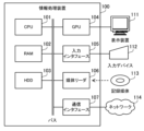
- FIG. 2 is a diagram showing an example of hardware of an information processing device according to the second embodiment.
- the information processing device 100 has a CPU 101, a RAM 102, a HDD 103, a GPU 104, an input interface 105, a media reader 106, and a communication interface 107, all connected to a bus.
- the CPU 101 corresponds to the control unit 12 in the first embodiment.
- the RAM 102 or the HDD 103 corresponds to the storage unit 11 in the first embodiment.
- the CPU 101 is a processor that executes program instructions.
- the CPU 101 loads the programs and data stored in the HDD 103 into the RAM 102 and executes the programs.
- the information processing device 100 may have multiple processors.
- RAM 102 is a volatile semiconductor memory that temporarily stores programs executed by CPU 101 and data used in calculations by CPU 101.
- Information processing device 100 may also have a type of volatile memory other than RAM.
- the HDD 103 is a non-volatile storage that stores software programs such as an operating system (OS), middleware, and application software, as well as data.
- the information processing device 100 may also have other types of non-volatile storage, such as flash memory or an SSD (Solid State Drive).
- the GPU 104 works in cooperation with the CPU 101 to perform image processing and output images to a display device 111 connected to the information processing device 100.
- the display device 111 is, for example, a CRT (Cathode Ray Tube) display, a liquid crystal display, an organic EL (Electro Luminescence) display, or a projector. Other types of output devices, such as a printer, may also be connected to the information processing device 100.
- the GPU 104 may also be used as a General Purpose Computing on Graphics Processing Unit (GPGPU).
- the GPU 104 may execute a program in response to an instruction from the CPU 101.
- the information processing device 100 may have a volatile semiconductor memory other than the RAM 102 as a GPU memory.
- the input interface 105 receives an input signal from an input device 112 connected to the information processing device 100.
- the input device 112 is, for example, a mouse, a touch panel, or a keyboard. Multiple input devices may be connected to the information processing device 100.
- the media reader 106 is a reading device that reads the programs and data recorded on the recording medium 113.
- the recording medium 113 is, for example, a magnetic disk, an optical disk, or a semiconductor memory. Magnetic disks include flexible disks (FDs) and HDDs. Optical disks include compact discs (CDs) and digital versatile discs (DVDs).
- the media reader 106 copies the programs and data read from the recording medium 113 to other recording media such as the RAM 102 or the HDD 103.
- the read programs may be executed by the CPU 101.
- the recording medium 113 may be a portable recording medium.
- the recording medium 113 may be used for distributing programs and data.
- the recording medium 113 and the HDD 103 may also be referred to as computer-readable recording media.
- the communication interface 107 communicates with other information processing devices via the network 114.
- the communication interface 107 may be a wired communication interface connected to a wired communication device such as a switch or a router, or a wireless communication interface connected to a wireless communication device such as a base station or an access point.
- the autoencoder of the second embodiment has isometry, which means that the distance in the latent space is proportional to the distance in the input data.
- This autoencoder may be called a variational autoencoder (VAE).
- VAE variational autoencoder
- RaDOGAGA RaDOGAGA (Rate-Distortion Optimization Guided Autoencoder for Generative Analysis).
- RaDOGAGA is also described in the following non-patent literature: Keizo Kato, Jing Zhou, Tomotake Sasaki and Akira Nakagawa, "Rate-Distortion Optimization Guided Autoencoder for Isometric Embedding in Euclidean Latent Space", Proc. of the 37th International Conference on Machine Learning (ICML 2020), pp. 5166-5176, July 2020.
- Encoder 141 accepts input data 144 and converts the input data 144 into a latent variable vector.
- the latent variable vector is sometimes called feature data or a feature vector.
- Input data 144 is a vector including multiple dimensions. The number of dimensions of the latent variable vector is smaller than that of input data 144. Therefore, encoder 141 compresses input data 144 and represents the features of input data 144 with a small vector.
- the information processing device 100 inputs the latent variable vector with added noise to the decoder 142.
- the information processing device 100 calculates the error 146 between the input data 144 and the predicted data 145.
- the error 146 is calculated using a distance function D.
- the error 146 is the Euclidean distance between the input data 144 and the predicted data 145.
- a distance index other than the Euclidean distance may be used.
- the information processing device 100 generates multiple latent variable vectors by inputting each of the multiple data records included in the mini-batch to the encoder 141.
- the information processing device 100 adds noise to each of the multiple latent variable vectors.
- the information processing device 100 generates a certain number of data records corresponding to the predicted data 145 by inputting each of the multiple noise-added latent variable vectors to the decoder 142.
- a plurality of latent variable vectors generated from one mini-batch follow a probability distribution P ⁇ having a parameter ⁇ .
- the probability distribution P ⁇ is a normal distribution
- the parameter ⁇ includes a mean and a variance.
- the information processing device 100 fits the plurality of latent variable vectors to the normal distribution for each mini-batch to estimate the value of the parameter ⁇ .
- the loss function includes an error term that indicates the average error of multiple data records included in a mini-batch.
- the information processing device 100 updates the values of the parameters ⁇ and ⁇ for each mini-batch so that the value of the loss function becomes smaller.
- the information processing device 100 repeats the process of extracting a mini-batch, calculating the value of the loss function, and updating the values of the parameters ⁇ and ⁇ .
- the information processing device 100 may repeat the above process until the number of iterations reaches a certain number.
- the information processing device 100 may also repeat the above process until the values of the parameters ⁇ and ⁇ converge.
- the loss function includes a correction term in addition to the error term.
- the correction term calculates a probability indicating the likelihood that the latent variable vector follows a probability distribution P ⁇ .
- the correction term uses the probability distribution P ⁇ estimated for each mini-batch.
- the correction term indicates the average probability of multiple latent variable vectors corresponding to multiple data records included in the mini-batch. The larger the probability, the smaller the value of the loss function. Since the noise-added latent variable vector input to the decoder 142 has fluctuations of the noise width T, the probability indicated by the correction term is the integral of the probability density in a range of width T centered on the generated latent variable vector.
- Equation (1) is an example of the loss function used in the second embodiment.
- m is the mini-batch size
- X i is the i-th input data record included in the mini-batch
- X ⁇ i is the i-th predicted data record
- D is the distance function
- ⁇ is a hyperparameter that takes a positive value
- z i is a latent variable vector generated from X i .
- Q zi is the probability that a latent variable vector in the vicinity of z i appears in the latent space.
- D(X i , X ⁇ i ) corresponds to the error term
- - ⁇ logQ zi corresponds to the correction term.
- Equation (2) The probability Qzi is defined as in Equation (2).
- Equation (2) z is a latent variable as a random variable
- U(z) is a rectangular window function
- P ⁇ (z) is a probability density function.
- the rectangular window function U(z) is defined as in Equation (3).
- Equation (3) zj is the element value of the jth dimension included in the argument vector. When the element values of all dimensions are greater than -T/2 and less than T/2, the rectangular window function U(z) outputs 1. When the element value of at least one dimension is not included in the above numerical range, the rectangular window function U(z) outputs 0.
- U(z ⁇ z i ) in formula (2) outputs 1 for latent variable vectors z within a range of T/2 from latent variable vector z i , and outputs 0 for other latent variable vectors z. Therefore, the probability Q zi is the probability obtained by integrating the probability density of latent variable vectors z within a range of T/2 from latent variable vector z i .
- the correction term reduces the value of the loss function.
- the correction term increases the value of the loss function. It can also be said that the correction term adds a penalty according to the latent variable vector to the error term.
- the probability distribution of the latent space may become a multimodal distribution with multiple probability density peaks.
- a multimodal distribution is expressed, for example, by a Gaussian mixture model.
- a Gaussian mixture model expresses a probability distribution as a weighted sum of multiple normal distributions. In that case, it may be preferable for the probability distribution of the latent space to also be a multimodal distribution. Expressing the latent space as a multimodal distribution may also improve the accuracy of the isometricity of the latent space.
- FIG. 4 is a diagram showing an example of how an autoencoder is used.
- One example of input data input to the encoder 141 is image data.
- the encoder 141 converts the image data into a latent variable vector whose data size is much smaller than that of the image data.
- the decoder 142 reproduces the image data from the latent variable vector.
- the encoder 141 generates a latent variable vector 153 from the input image data 151.
- the encoder 141 also generates a latent variable vector 154 from the input image data 152.
- the user may analyze the characteristics of the input image data group including the input image data 151 and 152 by looking at the probability distribution of the latent variable vector group including the latent variable vectors 153 and 154.
- the user classifies the input image data into multiple clusters based on the probability distribution of the latent space.
- the user extracts common characteristics shared by similar input image data based on the probability distribution of the latent space.
- the decoder 142 generates predicted image data 155 from the latent variable vector 153.
- the predicted image data 155 is a prediction result of the input image data 151.
- the decoder 142 generates predicted image data 156 from the latent variable vector 154.
- the predicted image data 156 is a prediction result of the input image data 152. Note that, at the time of prediction, noise does not need to be added to the latent variable vector input to the decoder 142.
- the user may create image data that is different from the known input image data by inputting a latent variable vector similar to a known latent variable vector into the decoder 142. This increases the variety of image data. The user can also analyze the correspondence between the image data and the latent variables.
- the encoder 141 and the decoder 142 are trained together during training, but may be used separately during prediction.
- a machine learning model that estimates a probability distribution from observed data is sometimes called a generative model.
- An example of the input image data 151, 152 is a protein structure image showing the molecular structure of a protein. Because protein structures are extremely complex, it is difficult for users to directly analyze protein structure images. Therefore, users may analyze the characteristics of the protein structure using a probability distribution in a latent space.
- Various protein structures may include similar and dissimilar protein structures, and various protein structures may be classified into multiple clusters. Therefore, the probability distribution of a protein structure image may be a multimodal distribution. Furthermore, to analyze protein structures using a latent space, it is preferable that the latent space has isometry. Therefore, it is preferable that the encoder 141 and the decoder 142 are trained so that the probability distribution of the latent space becomes a multimodal distribution with isometry.
- the probability distribution of the latent space is a multi-peak distribution with isometric properties.
- a Gaussian mixture model is substituted into the probability density function P ⁇ (z) of the above-mentioned formula (2), it may be difficult for the information processing device 100 to analytically solve the probability Q zi .
- the integral of the product of a rectangular window function and multiple normal distributions is non-differentiable, and the probability Qzi is non-differentiable. Therefore, machine learning using backpropagation and stochastic gradient descent can be difficult.
- the latent variable z is a high-dimensional vector, it is difficult to analytically solve the probability Qzi , and it is also difficult to use a library that uses a table to approximate the probability.
- the information processing device 100 replaces the probability Qzi in the above-mentioned formula (2) with a differentiable approximation formula. To this end, the information processing device 100 approximates the rectangular window function U(z) in the above-mentioned formula (3) with a Gaussian window function G(z) shown in formula (4).
- d is the number of dimensions of the latent space
- Id is a unit matrix with d rows and d columns.
- N(z; ⁇ , ⁇ ) is a normal distribution with z as a random variable, ⁇ as a mean vector, and ⁇ as a variance-covariance matrix.
- ⁇ 2 is the variance defined as in formula (5) using the noise width T.
- the variance ⁇ 2 is the variance of the Gaussian window function G(z) and is set to be equal to the variance of the rectangular window function U(z) of width T.
- FIG. 5 is a diagram showing an example of a rectangular window function and a Gaussian window function.
- Curve 161 shows a rectangular window function U(z).
- Curve 162 shows a Gaussian window function G(z).
- the weights output by the Gaussian window function G(z) are values between 0 and 1.
- the Gaussian window function G(z) outputs a maximum value of 1.
- the weights output by the Gaussian window function G(z) decay as the argument value moves away from 0.
- the curve 162 has the shape of a normal distribution, its amplitude differs from the probability density of a normal distribution.
- the output of G(z) is a constant multiple of the probability density defined by a normal distribution with mean 0 and variance ⁇ 2 .
- C is the number of clusters.
- One cluster that appears in the latent space is represented by one normal distribution. Therefore, C corresponds to the number of normal distributions.
- ⁇ c is a mixing coefficient indicating the weight of the c-th normal distribution
- ⁇ c is the mean vector of the c-th normal distribution
- ⁇ c is the variance-covariance matrix of the c-th normal distribution.
- Equation (4) By applying Equation (4) to G(z ⁇ z i ) in Equation (6) and expanding the product of normal distributions and integral operations, the probability Q zi is finally approximated as in Equation (7).
- the window function and integral operations have disappeared from the approximation equation for the probability Q zi .
- the approximation formula indicates that the probabilities indicated by C normal distributions for the latent variable vector z i are weighted by a mixing coefficient ⁇ c and summed up, and has the form of a mixed Gaussian model.
- the probability of each normal distribution is multiplied by a constant.
- the variance of each normal distribution is increased by ⁇ 2. Therefore, the approximation formula includes multiple normal distributions, each of which has a variance ⁇ 2 according to the noise width T.
- the approximation formula of the probability Qzi shown in Equation (7) is in a closed form and therefore can be differentiated.
- a closed form is a formula that combines differentiable basic functions such as addition, multiplication, and exponential functions. Therefore, the loss function including the probability Qzi is differentiable, and the information processing device 100 can perform machine learning using the backpropagation method and the stochastic gradient descent method. As a result, the autoencoder 140 is trained so that the latent variable vector follows a multi-peak distribution with isometricity.
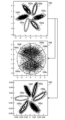
- FIG. 6 is a diagram showing an example of the correspondence between the input data space and the latent space.
- Graph 163 shows the probability distribution of the input data space.
- Graph 163 shows a multi-peak distribution including clusters 163a, 163b, 163c, 163d, 163e, and 163f.
- Graph 164 shows a probability distribution in the latent space obtained when probability Qzi is calculated using a single normal distribution.
- Graph 164 includes clusters 164a, 164b, 164c, 164d, 164e, and 164f.
- Cluster 164a corresponds to cluster 163a.
- Cluster 164b corresponds to cluster 163b.
- Cluster 164c corresponds to cluster 163c.
- Cluster 164d corresponds to cluster 163d.
- Cluster 164e corresponds to cluster 163e.
- Cluster 164f corresponds to cluster 163f.
- clusters 164a, 164b, 164c, 164d, 164e, and 164f form a unimodal distribution, not a multimodal distribution.
- similar latent variable vectors are generated from input data belonging to the same cluster, strictly speaking, isometry is not achieved. Therefore, there is room for improvement in the probability distribution of the latent space.
- a probability distribution expressed by a single normal distribution can also be interpreted as a mixture of a mixed probability distribution with a mixture number of 1.
- Graph 165 shows a probability distribution of a latent space obtained when the probability Qzi is calculated using a Gaussian mixture model.
- Graph 165 includes clusters 165a, 165b, 165c, 165d, 165e, and 165f.
- Cluster 165a corresponds to cluster 163a.
- Cluster 165b corresponds to cluster 163b.
- Cluster 165c corresponds to cluster 163c.
- Cluster 165d corresponds to cluster 163d.
- Cluster 165e corresponds to cluster 163e.
- Cluster 165f corresponds to cluster 163f.
- Clusters 165a, 165b, 165c, 165d, 165e, and 165f form a multi-modal distribution that corresponds to the input data space.
- isometry is achieved, in which the distance in the latent space is proportional to the distance in the input data space. Therefore, the probability distribution shown by graph 165 is useful for analyzing the characteristics of the input data.
- the value of the parameter ⁇ is updated for each mini-batch, and is updated multiple times during machine learning.
- the value of the parameter ⁇ may become unstable due to the randomness of the data records contained in the mini-batch.
- the information processing device 100 updates the value of the parameter ⁇ based on the formulas (8) to (10). At this time, the information processing device 100 also refers to the value of the parameter ⁇ calculated in the previous mini-batch.
- the parameter ⁇ includes a mixing coefficient ⁇ c , a mean vector ⁇ c and a variance-covariance matrix ⁇ c of each of the C normal distributions.
- the information processing device 100 first updates the mixing coefficient ⁇ c according to the formula (8), then updates the mean vector ⁇ c according to the formula (9), and finally updates the variance-covariance matrix ⁇ c according to the formula (10).
- ⁇ (l) c is the mixing coefficient of the c-th normal distribution calculated in the l-th iteration
- ⁇ (l-1) c is the mixing coefficient of the c-th normal distribution calculated in the l-1-th iteration
- ⁇ is a hyperparameter that takes a value between 0 and 1, and indicates the weight of the previous iteration. For example, ⁇ is between 0.95 and 0.99.
- p i,c is the probability that the latent variable vector z i belongs to the c-th normal distribution.
- the encoder 141 outputs a C-dimensional feature vector w i from the input data X i together with the d-dimensional latent variable vector z i .
- the feature vector w i is a vector that expresses the features of the input data X i in C dimensions.
- the information processing device 100 inputs the element values of each dimension of the feature vector w i to a softmax function to calculate the probability of belonging p i,c that takes a value between 0 and 1.
- ⁇ (l) c is the mean vector of the c-th normal distribution calculated in the l-th iteration
- ⁇ (l-1) c is the mean vector of the c-th normal distribution calculated in the l-1-th iteration
- ⁇ (l) c is the variance-covariance matrix of the c-th normal distribution calculated in the l-th iteration
- the information processing device 100 gradually updates the value of the parameter ⁇ based on the value of the parameter ⁇ calculated in the previous mini-batch. Therefore, the value of the parameter ⁇ is stable over multiple mini-batches, and the risk that the values of the parameters ⁇ and ⁇ will fall into a local solution is reduced.
- FIG. 7 is a block diagram showing an example of functions of the information processing device.
- the information processing device 100 has a training data storage unit 121, a hyperparameter storage unit 122, a model storage unit 123, a machine learning unit 124, and a prediction unit 125.
- the training data storage unit 121, the hyperparameter storage unit 122, and the model storage unit 123 are implemented using, for example, the RAM 102, the GPU memory, or the HDD 103.
- the machine learning unit 124 and the prediction unit 125 are implemented using, for example, the CPU 101 or the GPU 104, and a program.
- the training data storage unit 121 stores a training dataset.
- the training dataset includes a plurality of data records.
- the training dataset includes a plurality of image data records. Each data record does not need to be assigned a label.
- the hyperparameter storage unit 122 stores the values of hyperparameters used in machine learning.
- the values of the hyperparameters are specified, for example, by a user.
- the values of the hyperparameters are specified before the start of machine learning.
- the model storage unit 123 stores a trained autoencoder as a trained machine learning model.
- the trained autoencoder includes an encoder and a decoder that are trained in combination.
- the machine learning unit 124 trains the autoencoder using the training dataset stored in the training data storage unit 121 and the values of the hyperparameters stored in the hyperparameter storage unit 122. At this time, the machine learning unit 124 extracts mini-batches from the training dataset, inputs each data record included in the mini-batch to the autoencoder to calculate the value of the loss function, and updates the parameter values of the autoencoder by feeding back the value of the loss function. The machine learning unit 124 repeats the above process.
- the machine learning unit 124 stores the trained autoencoder in the model storage unit 123.
- the machine learning unit 124 may display the trained autoencoder on the display device 111, or may transmit it to another information processing device.
- the prediction unit 125 reads out the autoencoder from the model storage unit 123.
- the prediction unit 125 performs prediction processing using an encoder or a decoder in response to input from a user. For example, the prediction unit 125 inputs specified input data to an encoder and extracts features of the input data.
- the prediction unit 125 also inputs a specified latent variable vector to a decoder and generates prediction data having the latent variable vector as a feature.
- the prediction unit 125 may store the results of the prediction processing in non-volatile storage, may display the results on the display device 111, or may transmit the results to another information processing device.
- FIG. 8 is a diagram showing an example of the structure of a hyperparameter table.
- the hyperparameter table 131 is stored in the hyperparameter storage unit 122.
- the hyperparameter table 131 registers hyperparameter values of multiple hyperparameters.
- the hyperparameters include a noise width T, a loss function coefficient ⁇ , a probability distribution coefficient ⁇ , the number of clusters C, a mini-batch size m, and a distance function D.
- the noise width T adjusts the magnitude of noise added to the latent variable vector during machine learning.
- the loss function coefficient ⁇ is the weight of the correction term compared to the error term included in the loss function.
- the probability distribution coefficient ⁇ adjusts the amount of update per time when updating the value of the parameter ⁇ of the probability distribution P ⁇ .
- the number of clusters C is the number of types of input data.
- the mini-batch size m is the number of data records included in one mini-batch.
- the distance function D is a function that calculates the error between the input data and the predicted data, for example, calculating the Euclidean distance.
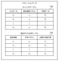
- FIG. 9 is a diagram showing an example of the structure of iteration data.
- the iteration data generated for each mini-batch includes a mini-batch table 132 and a Gaussian mixture table 133.
- the mini-batch table 132 and the Gaussian mixture table 133 are generated by the machine learning unit 124.
- the mini-batch table 132 associates input data X1 , X2 , ..., Xm , latent variable vectors z1 , z2 , ..., zm, and predicted data X ⁇ 1 , X ⁇ 2 , ..., X ⁇ m .
- a latent variable vector zi is generated by inputting input data Xi to an encoder.
- Predicted data Xi is generated by adding noise to the latent variable vector zi and inputting the result to a decoder.
- the Gaussian mixture distribution table 133 associates the mixing coefficients ⁇ 1 , ⁇ 2 , ..., ⁇ C with the mean vectors ⁇ 1 , ⁇ 2 , ..., ⁇ C and the variance-covariance matrices ⁇ 1 , ⁇ 2 , ..., ⁇ C.
- the mixing coefficients ⁇ c , the mean vector ⁇ c and the variance-covariance matrix ⁇ c are calculated from ⁇ c , ⁇ c , ⁇ c of the previous iteration and the latent variable vectors z 1 , z 2 , ..., z m of the current iteration.
- FIG. 10 is a flowchart showing an example of a machine learning procedure.
- the machine learning unit 124 acquires hyperparameter values. For example, the machine learning unit 124 reads out the hyperparameter values from the hyperparameter table 131.
- the hyperparameters include T, ⁇ , ⁇ , C, m, and D (S10).
- the machine learning unit 124 initializes the parameter values of the encoder and decoder included in the autoencoder (S11).
- the machine learning unit 124 extracts input data of mini-batch size m from the training dataset. At this time, it is preferable that the machine learning unit 124 preferentially extracts unused input data (S12).
- the machine learning unit 124 generates a latent variable vector from the input data using an encoder (S13).
- the machine learning unit 124 adds noise to the latent variable vector. At this time, the machine learning unit 124 adds noise randomly selected from a uniform distribution between -T/2 and T/2 to each dimension included in the latent variable vector (S14).
- the machine learning unit 124 generates prediction data from the noise-added latent variable vector using a decoder (S15).
- the machine learning unit 124 updates the mixed Gaussian distribution based on the mixed Gaussian distribution of the previous iteration and the latent variable vector generated in step S13. However, in the first iteration, the machine learning unit 124 estimates the mixed Gaussian distribution based on the latent variable vector generated in step S13 (S16).
- the machine learning unit 124 modifies the Gaussian mixture distribution updated in step S16 using the variance ⁇ 2 calculated from the noise width T, thereby defining the probability Qzi and defining a correction term including the probability Qzi (S17).
- the machine learning unit 124 defines a loss function including an error term indicating the error between the input data and the predicted data, and the correction term of step S17 (S18).
- the machine learning unit 124 updates the parameter values of the encoder and decoder so that the value of the loss function in step S18 becomes smaller (S19).
- the machine learning unit 124 determines whether the number of iterations in steps S12 to S19 has reached a threshold. If the number of iterations has reached the threshold, processing proceeds to step S21, and if the number of iterations has not reached the threshold, processing returns to step S12 (S20).
- the machine learning unit 124 outputs the trained encoder and decoder.
- the machine learning unit 124 may store the encoder and decoder in non-volatile storage, may display them on the display device 111, or may transmit them to another information processing device (S21).
- the information processing device 100 of the second embodiment adds noise with a noise width T to the latent variable vector output by the encoder and inputs it to the decoder. This trains the autoencoder so that the latent variable z follows a certain probability distribution.
- the information processing device 100 adds a correction term indicating the probability within a range of width T centered on the generated latent variable vector to the loss function. This achieves isometry, where the distance between two latent variable vectors is proportional to the distance of the input data corresponding to the latent variable vector.
- the information processing device 100 expresses the probability distribution used for the correction term as a Gaussian mixture model. As a result, if the probability distribution of the input data is a multimodal distribution, the latent variable z also follows a multimodal distribution. Therefore, a latent space useful for analyzing the characteristics of the input data is achieved.
- the information processing device 100 approximates the rectangular window function used for the correction term with a Gaussian window function. This eliminates the window function and integral operation from the approximation formula of the correction term.
- the approximation formula multiplies the probability density of the original Gaussian mixture model by a constant, and increases the variance of the original Gaussian mixture model by the variance ⁇ 2 corresponding to the noise width T. Therefore, even when a Gaussian mixture model is used, the loss function becomes a differentiable function, making it easier to execute the backpropagation method or the stochastic gradient descent method.
- the information processing device 100 inherits the parameter values of the Gaussian mixture model from the previous iteration with the weights ⁇ . This stabilizes the Gaussian mixture model over multiple iterations, reducing the risk that the parameter values of the autoencoder fall into a local solution.
Landscapes
- Engineering & Computer Science (AREA)
- Physics & Mathematics (AREA)
- Theoretical Computer Science (AREA)
- General Health & Medical Sciences (AREA)
- Computing Systems (AREA)
- Biomedical Technology (AREA)
- Biophysics (AREA)
- Computational Linguistics (AREA)
- Data Mining & Analysis (AREA)
- Evolutionary Computation (AREA)
- Life Sciences & Earth Sciences (AREA)
- Molecular Biology (AREA)
- Artificial Intelligence (AREA)
- General Engineering & Computer Science (AREA)
- General Physics & Mathematics (AREA)
- Mathematical Physics (AREA)
- Software Systems (AREA)
- Health & Medical Sciences (AREA)
- Probability & Statistics with Applications (AREA)
- Image Analysis (AREA)
Abstract
入力データの分布に対応する特徴データの分布をもつオートエンコーダを生成する。 情報処理装置(10)は、データ(15)をエンコーダ(13)に入力してデータ(16)を生成する。情報処理装置(10)は、大きさが閾値以下のノイズをデータ(16)に付加してデータ(17)を生成する。情報処理装置(10)は、データ(17)をデコーダ(14)に入力してデータ(18)を生成する。情報処理装置(10)は、データ(15)とデータ(18)との間の誤差を示す誤差項と、閾値に応じた分散をそれぞれもつ複数の確率分布を用いてデータ(16)から算出される確率を示す補正項とを含む損失関数(19)に基づいて、エンコーダ(13)およびデコーダ(14)の訓練を実行する。
Description
本発明は機械学習プログラム、機械学習方法および情報処理装置に関する。
機械学習モデルの1つに、エンコーダとデコーダとを含むオートエンコーダ(自己符号化器)がある。エンコーダは、入力データを、入力データよりもサイズが小さい特徴データに変換する。デコーダは、特徴データから入力データを予測する。オートエンコーダは、入力データを圧縮するために用いられることがある。また、オートエンコーダは、入力データの特徴を分析するために用いられることがある。
なお、入力データからエンコーダを用いて確率分布の平均および分散を算出し、確率分布からランダムにサンプルを選択し、選択されたサンプルからデコーダを用いて入力データを予測する分類オートエンコーダが提案されている。また、オートエンコーダを用いて物理システムのイベントの発生を予測するイベント予測方法が提案されている。また、入力データをデータ量の小さい圧縮データに変換するための変分オートエンコーダを訓練する機械学習システムが提案されている。
また、オートエンコーダを訓練する学習装置が提案されている。提案の学習装置は、エンコーダを用いて入力データを特徴データに変換し、特徴データにノイズを付加し、デコーダを用いてノイズ付き特徴データを出力データに変換する。学習装置は、入力データと出力データとの間の誤差と、特徴データの確率分布の情報エントロピーとを最小化するように、オートエンコーダのパラメータと特徴データの確率分布とを訓練する。
また、機械学習モデルを用いて画像データを符号化する画像符号化装置が提案されている。提案の画像符号化装置は、画像データを潜在空間の特徴データに変換し、特徴データを量子化し、量子化特徴データをエントロピー符号化してビットストリームを生成する。
ユーザは、入力データの分布に対応する特徴データの分布をもつオートエンコーダを取得したいことがある。特徴データの分布がもつ性質として、ユーザは、2つの入力データの距離が大きいほど、当該2つの入力データに対応する2つの特徴データの距離が大きいことを期待することがある。この性質は、等長性と呼ばれることがある。また、ユーザは、入力データの分布が複数のピークをもつ多峰分布である場合、特徴データの分布も多峰分布であることを期待することがある。
しかし、オートエンコーダを訓練する従来の機械学習技術の中には、特徴データの分布が等長性をもち、かつ多峰分布であるようなオートエンコーダを生成する機械学習技術はなかった。そこで、1つの側面では、本発明は、入力データの分布に対応する特徴データの分布をもつオートエンコーダを生成することを目的とする。
1つの態様では、以下の処理をコンピュータに実行させることを特徴とする機械学習プログラムが提供される。第1のデータをエンコーダに入力して第2のデータを生成する。大きさが閾値以下のノイズを第2のデータに付加して第3のデータを生成する。第3のデータをデコーダに入力して第4のデータを生成する。第1のデータと第4のデータとの間の誤差を示す誤差項と、閾値に応じた第1の分散をそれぞれもつ複数の第1の確率分布を用いて第2のデータから算出される確率を示す補正項とを含む損失関数に基づいて、エンコーダおよびデコーダの訓練を実行する。また、1つの態様では、コンピュータが実行することを特徴とする機械学習方法が提供される。また、1つの態様では、記憶部と制御部とを有することを特徴とする情報処理装置が提供される。
1つの側面では、入力データの分布に対応する特徴データの分布をもつオートエンコーダが生成される。
本発明の上記および他の目的、特徴および利点は本発明の例として好ましい実施の形態を表す添付の図面と関連した以下の説明により明らかになるであろう。
本発明の上記および他の目的、特徴および利点は本発明の例として好ましい実施の形態を表す添付の図面と関連した以下の説明により明らかになるであろう。
以下、本実施の形態を図面を参照して説明する。まず、第1の実施の形態を説明する。図1は、第1の実施の形態の情報処理装置を説明するための図である。第1の実施の形態の情報処理装置10は、訓練データを用いてオートエンコーダを訓練する機械学習を実行する。情報処理装置10は、クライアント装置でもよいしサーバ装置でもよい。情報処理装置10が、コンピュータまたは機械学習装置と呼ばれてもよい。
情報処理装置10は、記憶部11および制御部12を有する。記憶部11は、RAM(Random Access Memory)などの揮発性半導体メモリでもよい。また、記憶部11は、HDD(Hard Disk Drive)やフラッシュメモリなどの不揮発性ストレージでもよい。
制御部12は、例えば、CPU(Central Processing Unit)、GPU(Graphics Processing Unit)、DSP(Digital Signal Processor)などのプロセッサである。ただし、制御部12が、ASIC(Application Specific Integrated Circuit)やFPGA(Field Programmable Gate Array)などの電子回路を含んでもよい。プロセッサは、例えば、RAMなどのメモリ(記憶部11でもよい)に記憶されたプログラムを実行する。プロセッサの集合が、マルチプロセッサまたは単に「プロセッサ」と呼ばれてもよい。
記憶部11は、オートエンコーダに含まれるエンコーダ13およびデコーダ14を記憶する。オートエンコーダ、エンコーダ13およびデコーダ14が、機械学習モデルと呼ばれてもよい。エンコーダ13およびデコーダ14はそれぞれ、機械学習によって値が更新されるパラメータを含む。エンコーダ13およびデコーダ14は、例えば、複数の層を含むニューラルネットワークである。その場合、エンコーダ13およびデコーダ14に含まれるパラメータは、例えば、隣接する層の間のエッジの重みである。エンコーダ13およびデコーダ14のパラメータ値は、例えば、訓練開始時に初期化される。
エンコーダ13は、入力データを、入力データよりサイズの小さい特徴データに変換する。特徴データは、例えば、入力データより次元の少ない特徴ベクトルである。特徴データが、潜在変数データまたは潜在変数ベクトルと呼ばれることがある。デコーダ14は、特徴データを、特徴データよりサイズの大きい出力データに変換する。エンコーダ13と組み合わせて訓練されたデコーダ14は、特徴データから入力データを予測する。
入力データの種類としては、様々なものが考えられる。入力データは、画像データでもよいし、音声データでもよいし、自然言語データでもよいし、その他の測定データでもよい。よって、オートエンコーダは、画像処理モデルでもよいし、音声処理モデルでもよいし、自然言語処理モデルでもよいし、測定データ分析モデルでもよい。
情報処理装置10は、入力データの分布に対応する特徴データの分布をもつように、エンコーダ13およびデコーダ14を訓練する。特徴データの分布に期待される性質には、等長性および多峰性が含まれる。等長性は、入力データ上の相対的な距離が特徴データ上でも保存されることである。よって、2つの入力データの距離が大きいほど、当該2つの入力データに対応する2つの特徴データの距離も大きい。
多峰性は、特徴データの分布が、出現確率について複数のピークをもつ多峰分布であることである。入力データは複数の種類に分類されることがあり、入力データの分布は複数の種類に対応する複数のピークをもつ多峰分布であることがある。その場合、特徴データの分布も多峰分布であることが好ましいことがある。等長性および多峰性をもつオートエンコーダは、例えば、入力データの特徴を分析する際に有用である。
制御部12は、訓練データを用いてエンコーダ13およびデコーダ14を訓練する。訓練データは、ラベルが付与されていない教師なしデータであってもよい。制御部12は、データ15をエンコーダ13に入力することで、データ15からデータ16を生成する。データ15は入力データに相当し、データ16は特徴データに相当する。
制御部12は、大きさが閾値以下のノイズをデータ16に付加することで、データ16からデータ17を生成する。データ17は、ノイズ付き特徴データに相当する。データ16が複数の次元を含むベクトルである場合、例えば、制御部12は、各次元の要素値に、大きさが閾値以下のランダムなノイズ値を加算する。例えば、制御部12は、絶対値が閾値以下の数値範囲をもつ一様分布の中から、ランダムにノイズ値を選択する。
制御部12は、データ17をデコーダ14に入力することで、データ17からデータ18を生成する。データ18は出力データに相当し、データ15の予測結果と解釈される。制御部12は、データ15,16,18と損失関数19とに基づいて、エンコーダ13およびデコーダ14の訓練を実行する。このとき、制御部12は、損失関数19の値が小さくなるように、エンコーダ13およびデコーダ14のパラメータ値を更新する。
損失関数19の値は、損失(ロス)と呼ばれてもよい。損失関数19は、誤差関数、コスト関数または目的関数と呼ばれてもよい。制御部12は、誤差逆伝播法によって、デコーダ14の末尾からエンコーダ13の先頭に向かって損失情報を伝搬してもよい。また、制御部12は、確率的勾配降下法によってパラメータ値を更新してもよい。
損失関数19は、誤差項および補正項を含む。誤差項は、データ15とデータ18との間の誤差を示す。誤差は、例えば、距離関数を用いて算出される。距離は、例えば、ユークリッド距離である。補正項は、ある確率分布のもとでデータ16に対して算出される確率を示す。第1の実施の形態の補正項は、ノイズに関する上記の閾値に応じた分散をそれぞれもつ複数の確率分布を使用する。例えば、補正項は、複数の確率分布によってデータ16に対して算出される複数の確率の重み付き和を規定する。
各確率分布は正規分布(ガウス分布)であってもよく、複数の確率分布は混合ガウスモデル(GMM:Gaussian Mixture Model)を形成してもよい。複数の確率分布の重ね合わせは、確率密度のピーク(極大点)が複数ある多峰分布を表現することができる。ピークは、周辺の点よりも大きい確率密度をもつ頂点である。
複数の確率分布は、エンコーダ13の出力に基づいて推定されてもよい。補正項が示す確率は、例えば、潜在空間においてデータ16から上記の閾値の範囲内にある特徴データの確率密度、すなわち、データ16の近傍の確率密度を積分した確率の近似値である。誤差項が示す誤差が小さいほど、損失関数19の値は小さくなる。補正項が示す確率が大きいほど、損失関数19の値は小さくなる。補正項に負の符号が付されていてもよい。
補正項は、以下のようにして規定される近似式であってもよい。本来の補正項は、例えば、元の複数の確率分布それぞれから、矩形窓関数によってデータ16の近傍の確率密度を抽出し、抽出された近傍の確率密度を積分し、複数の確率分布に対応する複数の積分値の重み付き和を算出する。元の複数の確率分布は、幾つかの入力データからエンコーダ13によって変換された幾つかの特徴データにフィットするように推定される。
矩形窓関数は、データ16との差が前述の閾値未満である特徴データに対しては1を出力し、それ以外の特徴データに対しては0を出力する。データ16との差が閾値未満であるとは、例えば、ベクトルに含まれる全ての次元について、要素値の差の絶対値が閾値未満であることである。よって、各確率分布に矩形窓関数を乗じて積分することで、データ16との差が閾値未満である特徴データの確率密度を積分した近傍確率が算出される。
しかし、複数の確率分布に矩形窓関数を乗じて積分する本来の補正項は、微分不可能であることがあり、機械学習に用いることが難しいことがある。そこで、制御部12は、矩形窓関数をガウス型窓関数で近似する。ガウス型窓関数は、例えば、平均が0で、分散が矩形窓関数と同じである滑らかな確率密度関数である。ノイズの閾値がT/2(Tは正の定数)である場合、ガウス型窓関数の分散はT2/12である。ガウス型窓関数は、データ16との差が0である特徴データに対して、最大値の1を出力する。データ16との差が大きいほど、ガウス型窓関数の出力値が小さい。
矩形窓関数をガウス型窓関数で近似した場合、近似式を展開することで、近似式から窓関数および積分演算が消去される。近似された補正項は微分可能であり、機械学習に用いることが可能である。元の確率分布にガウス型窓関数を乗じて積分することで、元の確率分布の確率密度の大きさと分散とが修正される。確率密度は、元の確率分布の定数倍になる。分散は、元の確率分布よりも大きくなる。例えば、分散は、元の確率分布よりも、ガウス型窓関数の分散だけ大きくなる。よって、近似された補正項に含まれる各確率分布の分散は、ノイズの閾値に依存する。
以上説明したように、第1の実施の形態の情報処理装置10は、データ15をエンコーダ13に入力してデータ16を生成する。情報処理装置10は、大きさが閾値以下のノイズをデータ16に付加してデータ17を生成する。情報処理装置10は、データ17をデコーダ14に入力してデータ18を生成する。情報処理装置10は、誤差項と補正項とを含む損失関数19に基づいて、エンコーダ13およびデコーダ14の訓練を実行する。誤差項は、データ15とデータ18との間の誤差を示す。補正項は、閾値に応じた分散をそれぞれもつ複数の確率分布を用いてデータ16から算出される確率を示す。
ノイズの閾値に依存する補正項が損失関数19に含まれるため、訓練されたオートエンコーダが等長性を獲得する。また、補正項が複数の確率分布の重ね合わせを示すため、入力データの分布が多峰分布である場合、特徴データの分布も多峰分布になる。よって、入力データの特徴を分析する上で有用なオートエンコーダが獲得される。
また、ノイズの閾値に応じた分散をそれぞれもつ複数の確率分布を用いて補正項が近似されるため、損失関数19の値を小さくするようにエンコーダ13およびデコーダ14のパラメータ値を更新する機械学習の実行が容易となる。よって、入力データの分布に対応する特徴データの分布をもつオートエンコーダが獲得される。
なお、情報処理装置10は、データ16に基づいて複数の第2の確率分布を推定してもよく、ノイズの閾値に基づいて複数の第2の確率分布を、補正項に含まれる複数の第1の確率分布に変換してもよい。これにより、機械学習を通じて、エンコーダ13およびデコーダ14に加えて特徴データの分布も最適化される。
また、情報処理装置10は、ノイズに閾値に応じた第3の分散を、上記の複数の第2の確率分布がもつ第2の分散にそれぞれ加えることで、上記の複数の第1の確率分布がもつ第1の分散を算出してもよい。これにより、損失関数19を用いた機械学習が容易になるように補正項が近似される。また、第3の分散は、入力値の絶対値が閾値未満である場合に1を出力し、絶対値が閾値以上である場合に0を出力する矩形窓関数の分散であってもよい。これにより、補正項は、矩形窓関数を用いて算出される確率を近似できる。
また、情報処理装置10は、データ16を生成する処理と、複数の第2の確率分布を推定する処理とを反復的に実行してもよい。この場合に、情報処理装置10は、第1のイテレーションで推定される複数の第2の確率分布を規定する第1のパラメータ値を、データ16に加えて、第1のイテレーションより前の第2のイテレーションで算出された第2のパラメータ値を用いて算出してもよい。これにより、推定される特徴データの分布が安定し、推定精度が向上する。また、特徴データの分布の収束が早くなる。
次に、第2の実施の形態を説明する。第2の実施の形態の情報処理装置100は、訓練データを用いてオートエンコーダを訓練する機械学習を実行する。また、情報処理装置100は、訓練されたオートエンコーダに含まれるエンコーダまたはデコーダを利用する予測処理を実行する。ただし、機械学習と予測処理とが別の情報処理装置によって実行されてもよい。情報処理装置100は、クライアント装置でもよいしサーバ装置でもよい。情報処理装置100が、コンピュータまたは機械学習装置と呼ばれてもよい。情報処理装置100は、第1の実施の形態の情報処理装置10に対応する。
図2は、第2の実施の形態の情報処理装置のハードウェア例を示す図である。情報処理装置100は、バスに接続されたCPU101、RAM102、HDD103、GPU104、入力インタフェース105、媒体リーダ106および通信インタフェース107を有する。CPU101は、第1の実施の形態の制御部12に対応する。RAM102またはHDD103は、第1の実施の形態の記憶部11に対応する。
CPU101は、プログラムの命令を実行するプロセッサである。CPU101は、HDD103に記憶されたプログラムおよびデータをRAM102にロードし、プログラムを実行する。情報処理装置100は、複数のプロセッサを有してもよい。
RAM102は、CPU101で実行されるプログラムおよびCPU101で演算に使用されるデータを一時的に記憶する揮発性半導体メモリである。情報処理装置100は、RAM以外の種類の揮発性メモリを有してもよい。
HDD103は、オペレーティングシステム(OS:Operating System)やミドルウェアやアプリケーションソフトウェアなどのソフトウェアのプログラムと、データとを記憶する不揮発性ストレージである。情報処理装置100は、フラッシュメモリやSSD(Solid State Drive)などの他の種類の不揮発性ストレージを有してもよい。
GPU104は、CPU101と連携して画像処理を行い、情報処理装置100に接続された表示装置111に画像を出力する。表示装置111は、例えば、CRT(Cathode Ray Tube)ディスプレイ、液晶ディスプレイ、有機EL(Electro Luminescence)ディスプレイまたはプロジェクタである。情報処理装置100に、プリンタなどの他の種類の出力デバイスが接続されてもよい。
また、GPU104は、GPGPU(General Purpose Computing on Graphics Processing Unit)として使用されてもよい。GPU104は、CPU101からの指示に応じてプログラムを実行し得る。情報処理装置100は、RAM102以外の揮発性半導体メモリをGPUメモリとして有してもよい。
入力インタフェース105は、情報処理装置100に接続された入力デバイス112から入力信号を受け付ける。入力デバイス112は、例えば、マウス、タッチパネルまたはキーボードである。情報処理装置100に複数の入力デバイスが接続されてもよい。
媒体リーダ106は、記録媒体113に記録されたプログラムおよびデータを読み取る読み取り装置である。記録媒体113は、例えば、磁気ディスク、光ディスクまたは半導体メモリである。磁気ディスクには、フレキシブルディスク(FD:Flexible Disk)およびHDDが含まれる。光ディスクには、CD(Compact Disc)およびDVD(Digital Versatile Disc)が含まれる。媒体リーダ106は、記録媒体113から読み取られたプログラムおよびデータを、RAM102やHDD103などの他の記録媒体にコピーする。読み取られたプログラムは、CPU101によって実行されることがある。
記録媒体113は、可搬型記録媒体であってもよい。記録媒体113は、プログラムおよびデータの配布に用いられることがある。また、記録媒体113およびHDD103が、コンピュータ読み取り可能な記録媒体と呼ばれてもよい。
通信インタフェース107は、ネットワーク114を介して他の情報処理装置と通信する。通信インタフェース107は、スイッチやルータなどの有線通信装置に接続される有線通信インタフェースでもよいし、基地局やアクセスポイントなどの無線通信装置に接続される無線通信インタフェースでもよい。
次に、オートエンコーダについて説明する。第2の実施の形態のオートエンコーダは、潜在空間上の距離が入力データ上の距離に比例するという等長性をもつ。このオートエンコーダが、変分オートエンコーダ(VAE:Variational Autoencoder)と呼ばれてもよい。等長性をもつオートエンコーダの一例として、RaDOGAGA(Rate-Distortion Optimization Guided Autoencoder for Generative Analysis)がある。
RaDOGAGAは、次の非特許文献にも記載されている。Keizo Kato, Jing Zhou, Tomotake Sasaki and Akira Nakagawa, "Rate-Distortion Optimization Guided Autoencoder for Isometric Embedding in Euclidean Latent Space", Proc. of the 37th International Conference on Machine Learning (ICML 2020), pp. 5166-5176, July 2020。
図3は、オートエンコーダの構造例を示す図である。オートエンコーダ140は、エンコーダ141およびデコーダ142を含む。エンコーダ141およびデコーダ142はそれぞれ、複数の層を含むニューラルネットワークである。エンコーダ141は、パラメータθを含む関数fθとして表現される。デコーダ142は、パラメータφを含む関数gφとして表現される。パラメータθ,φには、隣接する層の間のエッジの重みが含まれる。パラメータθ,φの値は、機械学習を通じて算出される。
エンコーダ141は、入力データ144を受け付け、入力データ144を潜在変数ベクトルに変換する。潜在変数ベクトルは、特徴データまたは特徴ベクトルと呼ばれることがある。入力データ144は、複数の次元を含むベクトルである。潜在変数ベクトルの次元数は、入力データ144よりも小さい。よって、エンコーダ141は、入力データ144を圧縮して、入力データ144の特徴を小さいベクトルで表現する。
デコーダ142は、潜在変数ベクトルを受け付け、潜在変数ベクトルを予測データ145に変換する。予測データ145は、複数の次元を含むベクトルである。予測データ145の次元数は、潜在変数ベクトルよりも大きく、通常は入力データ144と同じである。エンコーダ141が出力する潜在変数ベクトルをデコーダ142に入力した場合、予測データ145は、入力データ144の予測結果を示す。
潜在変数ベクトルが一定の確率分布に従うようにするため、情報処理装置100は、オートエンコーダ140の訓練時にサンプリング部143を使用する。サンプリング部143は、エンコーダ141が出力する潜在変数ベクトルの各次元にランダムなノイズを加算する。ノイズは、-T/2以上T/2以下の数値範囲をもつ一様分布からランダムに選択される。一様分布は、全ての事象が等確率で発生することを示す確率分布である。Tは、正の値をとるハイパーパラメータであり、ノイズ幅を示す。
情報処理装置100は、ノイズが付加された潜在変数ベクトルをデコーダ142に入力する。情報処理装置100は、入力データ144と予測データ145との間の誤差146を算出する。誤差146は、距離関数Dを用いて算出される。例えば、誤差146は、入力データ144と予測データ145との間のユークリッド距離である。ただし、ユークリッド距離以外の距離指標が使用されてもよい。
情報処理装置100は、誤差146を含む損失関数の値が小さくなるように、パラメータθ,φの値を更新する。例えば、情報処理装置100は、誤差逆伝播法により、デコーダ142の末尾からエンコーダ141の先頭に向かって損失情報を伝搬する。例えば、情報処理装置100は、確率的勾配降下法により、損失情報とパラメータθ,φの現在値とから勾配を算出し、算出された勾配を用いてパラメータθ,φの値を更新する。潜在変数ベクトルにノイズが付加されることで、潜在空間が一定の確率分布を形成する。
パラメータθ,φの値の更新は、入力データ144に相当する一定個数のデータレコードを含むミニバッチ単位で行われる。ミニバッチは、事前に用意された訓練データセットから抽出される。訓練データセットの各データレコードにはラベルが付与されていなくてもよく、オートエンコーダ140の機械学習は教師なし学習であってもよい。
情報処理装置100は、ミニバッチに含まれる複数のデータレコードをそれぞれエンコーダ141に入力することで、複数の潜在変数ベクトルを生成する。情報処理装置100は、複数の潜在変数ベクトルにそれぞれノイズを付加する。情報処理装置100は、複数のノイズ付き潜在変数ベクトルをそれぞれデコーダ142に入力することで、予測データ145に相当する一定個数のデータレコードを生成する。
1つのミニバッチから生成される複数の潜在変数ベクトルは、パラメータψをもつ確率分布Pψに従う。例えば、確率分布Pψは正規分布であり、パラメータψは平均および分散を含む。情報処理装置100は、ミニバッチ毎に、複数の潜在変数ベクトルを正規分布にフィッティングして、パラメータψの値を推定する。
損失関数は、ミニバッチに含まれる複数のデータレコードの平均誤差を示す誤差項を含む。情報処理装置100は、ミニバッチ毎に、損失関数の値が小さくなるようにパラメータθ,φの値を更新する。情報処理装置100は、ミニバッチを抽出し、損失関数の値を算出し、パラメータθ,φの値を更新することを繰り返す。情報処理装置100は、反復回数が一定回数に達するまで上記の処理を繰り返してもよい。また、情報処理装置100は、パラメータθ,φの値が収束するまで上記の処理を繰り返してもよい。
ここで、潜在空間が等長性をもつようにするため、損失関数は、誤差項に加えて補正項を含む。補正項は、潜在変数ベクトルが確率分布Pψに従っている確からしさを示す確率を算出する。補正項は、ミニバッチ毎に推定される確率分布Pψを使用する。補正項は、ミニバッチに含まれる複数のデータレコードに対応する複数の潜在変数ベクトルの平均確率を示す。確率が大きいほど、損失関数の値が小さくなる。デコーダ142に入力されるノイズ付き潜在変数ベクトルはノイズ幅Tの揺らぎをもつため、補正項が示す確率は、生成された潜在変数ベクトルを中心とする幅Tの範囲の確率密度の積分である。
次に、損失関数について更に説明する。数式(1)は、第2の実施の形態で使用される損失関数の例である。数式(1)において、mはミニバッチサイズ、Xiはミニバッチに含まれるi番目の入力データレコード、X^
iはi番目の予測データレコード、Dは距離関数、βは正の値をとるハイパーパラメータ、ziはXiから生成される潜在変数ベクトルである。Qziは、潜在空間においてziの近傍の潜在変数ベクトルが出現する確率である。D(Xi,X^
i)が誤差項に相当し、-βlogQziが補正項に相当する。

確率Qziは、数式(2)のように規定される。数式(2)において、zは確率変数としての潜在変数、U(z)は矩形窓関数、Pψ(z)は確率密度関数である。矩形窓関数U(z)は、数式(3)のように規定される。数式(3)において、zjは引数のベクトルに含まれるj番目の次元の要素値である。全ての次元の要素値が-T/2より大きくT/2より小さい場合、矩形窓関数U(z)は1を出力する。少なくとも1つの次元の要素値が上記の数値範囲に含まれない場合、矩形窓関数U(z)は0を出力する。


よって、数式(2)のU(z-zi)は、潜在変数ベクトルziからT/2の範囲内にある潜在変数ベクトルzに対して1を出力し、それ以外の潜在変数ベクトルzに対して0を出力する。そのため、確率Qziは、潜在変数ベクトルziからT/2の範囲内にある潜在変数ベクトルzの確率密度を積分した確率である。
潜在変数ベクトルziの近傍の確率が大きい場合、ziは確率分布Pψに十分に従っていると言える。そこで、補正項は、損失関数の値を小さくする。一方、潜在変数ベクトルziの近傍の確率が小さい場合、ziは確率分布Pψに十分に従っているとは言えない。そこで、補正項は、損失関数の値を大きくする。補正項は、潜在変数ベクトルに応じたペナルティを誤差項に対して付加しているとも言える。
次に、潜在空間の確率分布を多峰分布にすることを考える。入力データが複数のクラスタに分類される場合、入力データの確率分布は、確率密度のピークが複数個ある多峰分布になることがある。多峰分布は、例えば、混合ガウスモデルで表現される。混合ガウスモデルは、確率分布を、複数の正規分布の重み付き和で表現する。その場合、潜在空間の確率分布も多峰分布になることが好ましいことがある。潜在空間を多峰分布で表現することで、潜在空間の等長性の精度も向上し得る。
図4は、オートエンコーダの使用例を示す図である。エンコーダ141に入力される入力データの一例として、画像データが挙げられる。エンコーダ141は、画像データを、画像データよりもデータサイズが十分に小さい潜在変数ベクトルに変換する。デコーダ142は、潜在変数ベクトルから画像データを再現する。
例えば、エンコーダ141は、入力画像データ151から潜在変数ベクトル153を生成する。また、エンコーダ141は、入力画像データ152から潜在変数ベクトル154を生成する。ユーザは、潜在変数ベクトル153,154を含む潜在変数ベクトル群の確率分布を見ることで、入力画像データ151,152を含む入力画像データ群の特徴を分析することがある。例えば、ユーザは、潜在空間の確率分布に基づいて、入力画像データを複数のクラスタに分類する。また、例えば、ユーザは、潜在空間の確率分布に基づいて、類似する入力画像データがもつ共通の特徴を抽出する。
また、例えば、デコーダ142は、潜在変数ベクトル153から予測画像データ155を生成する。予測画像データ155は、入力画像データ151の予測結果である。また、デコーダ142は、潜在変数ベクトル154から予測画像データ156を生成する。予測画像データ156は、入力画像データ152の予測結果である。なお、予測時には、デコーダ142に入力される潜在変数ベクトルにノイズが付加されなくてもよい。
ユーザは、既知の潜在変数ベクトルに類似する潜在変数ベクトルをデコーダ142に入力することで、既知の入力画像データと異なる画像データを作成することがある。これにより、画像データのバリエーションが増える。また、ユーザは、画像データと潜在変数との対応関係を分析することができる。
このように、エンコーダ141およびデコーダ142は、訓練時には組み合わせて訓練される一方、予測時にはそれぞれ単独で使用されることがある。なお、観測データから確率分布を推定する機械学習モデルは、生成モデルと呼ばれることがある。
入力画像データ151,152の一例として、タンパク質の分子構造を示すタンパク質構造画像が挙げられる。タンパク質構造は極めて複雑であるため、ユーザはタンパク質構造画像を直接的に分析することが難しい。そこで、ユーザは、潜在空間の確率分布を用いて、タンパク質構造の特徴を分析することがある。
種々のタンパク質構造の中には類似するタンパク質構造と類似しないタンパク質構造とが含まれることがあり、種々のタンパク質構造は複数のクラスタに分類されることがある。よって、タンパク質構造画像の確率分布が、多峰分布であることがある。また、潜在空間を用いてタンパク質構造を分析するには、潜在空間が等長性をもつことが好ましい。そのため、潜在空間の確率分布が等長性のある多峰分布になるように、エンコーダ141およびデコーダ142が訓練されることが好ましい。
このように、オートエンコーダ140の機械学習においては、潜在空間の確率分布が等長性のある多峰分布になることが好ましい場合がある。しかし、前述の数式(2)の確率密度関数Pψ(z)に混合ガウスモデルを代入すると、情報処理装置100は、確率Qziを解析的に解くことが難しいことがある。
矩形窓関数と複数の正規分布との積の積分は微分不可能であり、確率Qziが微分不可能になる。そのため、誤差逆伝播法および確率的勾配降下法を用いた機械学習が難しいことがある。特に、潜在変数zが高次元ベクトルである場合、確率Qziを解析的に解くことが難しく、数表を用いて確率の近似値を求めるライブラリを利用することも難しい。
そこで、情報処理装置100は、前述の数式(2)の確率Qziを、微分可能な近似式に置換する。そのために、情報処理装置100は、前述の数式(3)の矩形窓関数U(z)を、数式(4)に示すガウス型窓関数G(z)で近似する。

数式(4)において、dは潜在空間の次元数、Idはd行d列の単位行列である。N(z;μ,Σ)は、zを確率変数としてもち、μを平均ベクトルとしてもち、Σを分散共分散行列としてもつ正規分布である。σ2は、ノイズ幅Tを用いて数式(5)のように規定される分散である。分散σ2は、ガウス型窓関数G(z)の分散であり、幅Tの矩形窓関数U(z)の分散と等しいように設定される。

図5は、矩形窓関数とガウス型窓関数の例を示す図である。曲線161は、矩形窓関数U(z)を示す。曲線162は、ガウス型窓関数G(z)を示す。図5では、T2=12でありσ2=1である場合を想定している。
ガウス型窓関数G(z)が出力する重みは、0以上1以下の数値である。ガウス型窓関数G(z)は、引数の値が0である場合に、最大値の1を出力する。ガウス型窓関数G(z)が出力する重みは、引数の値が0から離れるに従って減衰する。曲線162は正規分布の形状をもつものの、その振幅は正規分布の確率密度とは異なる。G(z)の出力は、平均が0で分散がσ2の正規分布によって規定される確率密度の定数倍である。
前述の数式(2)において、確率密度関数Pψ(z)に混合ガウスモデルを代入し、矩形窓関数に関するU(z-zi)をガウス型窓関数に関するG(z-zi)で近似した場合、確率Qziは数式(6)のように近似される。

数式(6)において、Cはクラスタ数である。潜在空間に出現する1つのクラスタは、1つの正規分布で表現される。よって、Cは正規分布の個数に相当する。πcはc番目の正規分布の重みを示す混合係数、μcはc番目の正規分布の平均ベクトル、Σcはc番目の正規分布の分散共分散行列である。
数式(6)のG(z-zi)に数式(4)を適用し、正規分布同士の積と積分演算とを展開すると、確率Qziは最終的に数式(7)のように近似される。確率Qziの近似式からは、窓関数および積分演算が消えている。

近似式は、潜在変数ベクトルziに対してC個の正規分布が示す確率を、混合係数πcで重み付けして合算することを示しており、混合ガウスモデルの形をもつ。ただし、ミニバッチから推定された元の混合ガウスモデルと異なり、各正規分布の確率が定数倍される。また、元の混合ガウスモデルと異なり、各正規分布の分散がσ2だけ大きくなる。よって、近似式は、ノイズ幅Tに応じた分散σ2をそれぞれもつ複数の正規分布を含む。
数式(7)に示す確率Qziの近似式は、閉形式であるため微分可能である。閉形式は、加算、乗算、指数関数などの微分可能な基本的関数を組み合わせた数式である。このため、確率Qziを含む損失関数が微分可能であり、情報処理装置100は、誤差逆伝播法および確率的勾配降下法を用いた機械学習を実行することができる。その結果、潜在変数ベクトルが等長性のある多峰分布に従うように、オートエンコーダ140が訓練される。
図6は、入力データ空間と潜在空間の対応例を示す図である。グラフ163は、入力データ空間の確率分布を示す。グラフ163は、クラスタ163a,163b,163c,163d,163e,163fを含む多峰分布を示す。
グラフ164は、単一の正規分布を用いて確率Qziを算出した場合に獲得される潜在空間の確率分布を示す。グラフ164は、クラスタ164a,164b,164c,164d,164e,164fを含む。クラスタ164aはクラスタ163aに対応する。クラスタ164bはクラスタ163bに対応する。クラスタ164cはクラスタ163cに対応する。クラスタ164dはクラスタ163dに対応する。クラスタ164eはクラスタ163eに対応する。クラスタ164fはクラスタ163fに対応する。
ただし、クラスタ164a,164b,164c,164d,164e,164fは、単峰分布を形成しており、多峰分布を形成していない。また、同じクラスタに属する入力データから類似する潜在変数ベクトルが生成されているものの、厳密には等長性が達成されていない。よって、潜在空間の確率分布に改善の余地がある。なお、単一の正規分布で表現される確率分布は、混合確率分布の混合数が1であると解釈することもできる。
グラフ165は、混合ガウスモデルを用いて確率Qziを算出した場合に獲得される潜在空間の確率分布を示す。グラフ165は、クラスタ165a,165b,165c,165d,165e,165fを含む。クラスタ165aはクラスタ163aに対応する。クラスタ165bはクラスタ163bに対応する。クラスタ165cはクラスタ163cに対応する。クラスタ165dはクラスタ163dに対応する。クラスタ165eはクラスタ163eに対応する。クラスタ165fはクラスタ163fに対応する。
クラスタ165a,165b,165c,165d,165e,165fは、入力データ空間に対応する多峰分布を形成している。また、潜在空間上の距離が入力データ空間上の距離に比例するという等長性が達成されている。よって、グラフ165が示す確率分布は、入力データの特徴を分析する上で有用である。
次に、確率分布Pψを規定するパラメータψの最適化について説明する。前述のように、パラメータψの値はミニバッチ毎に更新され、機械学習の間に複数回更新される。ここで、パラメータψの値を1回更新する際に、更新後の値を1つのミニバッチのみから算出すると、そのミニバッチに含まれるデータレコードの偶然性の影響を受けて、パラメータψの値が不安定になることがある。その結果、エンコーダ141を規定するパラメータθの値とデコーダ142を規定するパラメータφの値が、局所解に陥るリスクがある。
そこで、情報処理装置100は、数式(8)~(10)に基づいてパラメータψの値を更新する。このとき、情報処理装置100は、1つ前のミニバッチで算出されたパラメータψの値も参照する。パラメータψは、C個の正規分布それぞれの混合係数πc、平均ベクトルμcおよび分散共分散行列Σcを含む。情報処理装置100は、まず数式(8)に従って混合係数πcを更新し、次に数式(9)に従って平均ベクトルμcを更新し、最後に数式(10)に従って分散共分散行列Σcを更新する。



数式(8)において、π(l)
cはl回目のイテレーションで算出されるc番目の正規分布の混合係数、π(l-1)
cはl-1回目のイテレーションで算出されるc番目の正規分布の混合係数である。ξは0以上1以下の値をとるハイパーパラメータであり、前イテレーションの重みを示す。例えば、ξは0.95以上0.99以下である。
pi,cは、潜在変数ベクトルziがc番目の正規分布に帰属する確率である。エンコーダ141は、入力データXiから、d次元の潜在変数ベクトルziと併せてC次元の特徴ベクトルwiを出力する。特徴ベクトルwiは、入力データXiの特徴をC次元で表現したベクトルである。情報処理装置100は、特徴ベクトルwiの各次元の要素値をソフトマックス関数に入力することで、0以上1以下の値をとる帰属確率pi,cを算出する。
数式(9)において、μ(l)
cはl回目のイテレーションで算出されるc番目の正規分布の平均ベクトル、μ(l-1)
cはl-1回目のイテレーションで算出されるc番目の正規分布の平均ベクトルである。数式(10)において、Σ(l)
cはl回目のイテレーションで算出されるc番目の正規分布の分散共分散行列、Σ(l-1)
cはl-1回目のイテレーションで算出されるc番目の正規分布の分散共分散行列である。なお、初回イテレーションでは、ξ=0とみなしてπ(1)
c,μ(1)
c,Σ(1)
cが算出される。
このように、情報処理装置100は、前のミニバッチで算出されたパラメータψの値を元にして、パラメータψの値を緩やかに更新する。よって、複数のミニバッチを通してパラメータψの値が安定し、パラメータθ,φの値が局所解に陥るリスクが低下する。
次に、情報処理装置100の機能および処理手順について説明する。図7は、情報処理装置の機能例を示すブロック図である。情報処理装置100は、訓練データ記憶部121、ハイパーパラメータ記憶部122、モデル記憶部123、機械学習部124および予測部125を有する。訓練データ記憶部121、ハイパーパラメータ記憶部122およびモデル記憶部123は、例えば、RAM102、GPUメモリまたはHDD103を用いて実装される。機械学習部124および予測部125は、例えば、CPU101またはGPU104と、プログラムとを用いて実装される。
訓練データ記憶部121は、訓練データセットを記憶する。訓練データセットは、複数のデータレコードを含む。例えば、訓練データセットは、複数の画像データレコードを含む。各データレコードには、ラベルが付与されていなくてもよい。
ハイパーパラメータ記憶部122は、機械学習に使用されるハイパーパラメータの値を記憶する。ハイパーパラメータの値は、例えば、ユーザから指定される。ハイパーパラメータの値は、機械学習の開始前に指定される。モデル記憶部123は、訓練済みの機械学習モデルとして、訓練済みのオートエンコーダを記憶する。訓練済みのオートエンコーダは、組み合わせて訓練されたエンコーダとデコーダとを含む。
機械学習部124は、訓練データ記憶部121に記憶された訓練データセットと、ハイパーパラメータ記憶部122に記憶されたハイパーパラメータの値とを用いて、オートエンコーダを訓練する。このとき、機械学習部124は、訓練データセットからミニバッチを抽出し、ミニバッチに含まれる各データレコードをオートエンコーダに入力して損失関数の値を算出し、損失関数の値をフィードバックしてオートエンコーダのパラメータ値を更新する。機械学習部124は、上記の処理を反復する。
機械学習部124は、訓練されたオートエンコーダをモデル記憶部123に保存する。なお、機械学習部124は、訓練されたオートエンコーダを表示装置111に表示してもよいし、他の情報処理装置に送信してもよい。
予測部125は、モデル記憶部123からオートエンコーダを読み出す。予測部125は、ユーザからの入力に応じて、エンコーダまたはデコーダを用いて予測処理を行う。例えば、予測部125は、指定された入力データをエンコーダに入力することで、その入力データの特徴を抽出する。また、予測部125は、指定された潜在変数ベクトルをデコーダに入力することで、その潜在変数ベクトルを特徴としてもつ予測データを生成する。なお、予測部125は、予測処理の結果を不揮発性ストレージに保存してもよいし、表示装置111に表示してもよいし、他の情報処理装置に送信してもよい。
図8は、ハイパーパラメータテーブルの構造例を示す図である。ハイパーパラメータテーブル131は、ハイパーパラメータ記憶部122に記憶される。ハイパーパラメータテーブル131には、複数のハイパーパラメータのハイパーパラメータ値が登録される。ハイパーパラメータには、ノイズ幅T、損失関数係数β、確率分布係数ξ、クラスタ数C、ミニバッチサイズmおよび距離関数Dが含まれる。
ノイズ幅Tは、機械学習時に潜在変数ベクトルに付加されるノイズの大きさを調整する。損失関数係数βは、損失関数に含まれる誤差項と比べた補正項の重みである。確率分布係数ξは、確率分布Pψのパラメータψの値を更新する際の1回の更新量を調整する。クラスタ数Cは、入力データの種類数である。ミニバッチサイズmは、1つのミニバッチに含まれるデータレコードの個数である。距離関数Dは、入力データと予測データの間の誤差を算出する関数であり、例えば、ユークリッド距離を算出する。
図9は、イテレーションデータの構造例を示す図である。ミニバッチ毎に生成されるイテレーションデータには、ミニバッチテーブル132および混合ガウス分布テーブル133が含まれる。ミニバッチテーブル132および混合ガウス分布テーブル133は、機械学習部124によって生成される。
ミニバッチテーブル132は、入力データX1,X2,…,Xmと潜在変数ベクトルz1,z2,…,zmと予測データX^1,X^2,…,X^mとを対応付ける。入力データXiをエンコーダに入力することで、潜在変数ベクトルziが生成される。潜在変数ベクトルziにノイズを付加してデコーダに入力することで、予測データX^iが生成される。
混合ガウス分布テーブル133は、混合係数π1,π2,…,πCと平均ベクトルμ1,μ2,…,μCと分散共分散行列Σ1,Σ2,…,ΣCとを対応付ける。混合係数πc、平均ベクトルμcおよび分散共分散行列Σcは、前イテレーションのπc,μc,Σcと現イテレーションの潜在変数ベクトルz1,z2,…,zmとから算出される。
図10は、機械学習の手順例を示すフローチャートである。機械学習部124は、ハイパーパラメータ値を取得する。例えば、機械学習部124は、ハイパーパラメータテーブル131からハイパーパラメータ値を読み出す。ハイパーパラメータには、T,β,ξ,C,m,Dが含まれる(S10)。機械学習部124は、オートエンコーダに含まれるエンコーダおよびデコーダのパラメータ値を初期化する(S11)。
機械学習部124は、訓練データセットの中から、ミニバッチサイズmの入力データを抽出する。このとき、機械学習部124は、未使用の入力データを優先的に抽出することが好ましい(S12)。機械学習部124は、エンコーダを用いて入力データから潜在変数ベクトルを生成する(S13)。機械学習部124は、潜在変数ベクトルにノイズを付与する。このとき、機械学習部124は、潜在変数ベクトルに含まれる各次元に、-T/2以上T/2以下の一様分布からランダムに選択されたノイズを加算する(S14)。
機械学習部124は、デコーダを用いてノイズ付き潜在変数ベクトルから予測データを生成する(S15)。機械学習部124は、前イテレーションの混合ガウス分布と、ステップS13で生成された潜在変数ベクトルとに基づいて、混合ガウス分布を更新する。ただし、初回イテレーションでは、機械学習部124は、ステップS13で生成された潜在変数ベクトルに基づいて混合ガウス分布を推定する(S16)。
機械学習部124は、ノイズ幅Tから算出される分散σ2を用いて、ステップS16で更新された混合ガウス分布を修正することで、確率Qziを規定し、確率Qziを含む補正項を規定する(S17)。機械学習部124は、入力データと予測データとの間の誤差を示す誤差項と、ステップS17の補正項とを含む損失関数を規定する(S18)。
機械学習部124は、ステップS18の損失関数の値が小さくなるように、エンコーダおよびデコーダのパラメータ値を更新する(S19)。機械学習部124は、ステップS12~S19のイテレーション回数が閾値に達したか判断する。イテレーション回数が閾値に達した場合はステップS21に処理が進み、イテレーション回数が閾値に達していない場合はステップS12に処理が戻る(S20)。
機械学習部124は、訓練されたエンコーダおよびデコーダを出力する。機械学習部124は、エンコーダおよびデコーダを不揮発性ストレージに保存してもよいし、表示装置111に表示してもよいし、他の情報処理装置に送信してもよい(S21)。
以上説明したように、第2の実施の形態の情報処理装置100は、エンコーダが出力する潜在変数ベクトルにノイズ幅Tのノイズを付加してデコーダに入力する。これにより、潜在変数zが一定の確率分布に従うようにオートエンコーダが訓練される。
また、情報処理装置100は、生成された潜在変数ベクトルを中心とする幅Tの範囲内の確率を示す補正項を、損失関数に追加する。これにより、2つの潜在変数ベクトルの距離が、当該潜在変数ベクトルに対応する入力データの距離に比例するという等長性が獲得される。また、情報処理装置100は、補正項に使用する確率分布を混合ガウスモデルで表現する。これにより、入力データの確率分布が多峰分布である場合、潜在変数zも多峰分布に従う。よって、入力データの特徴を分析する上で有用な潜在空間が獲得される。
また、情報処理装置100は、補正項に使用する矩形窓関数をガウス型窓関数で近似する。これにより、補正項の近似式から窓関数や積分演算が消去される。近似式は、元の混合ガウスモデルの確率密度を定数倍し、元の混合ガウスモデルの分散をノイズ幅Tに対応する分散σ2だけ大きくする。よって、混合ガウスモデルを使用した場合であっても、損失関数が微分可能関数になり、誤差逆伝播法や確率的勾配降下法の実行が容易になる。
また、情報処理装置100は、現イテレーションのミニバッチのみから混合ガウスモデルを推定する代わりに、前イテレーションの混合ガウスモデルのパラメータ値を重みξで引き継ぐ。これにより、複数のイテレーションを通して混合ガウスモデルが安定し、オートエンコーダのパラメータ値が局所解に陥るリスクが低下する。
上記については単に本発明の原理を示すものである。更に、多数の変形や変更が当業者にとって可能であり、本発明は上記に示し、説明した正確な構成および応用例に限定されるものではなく、対応する全ての変形例および均等物は、添付の請求項およびその均等物による本発明の範囲とみなされる。
10 情報処理装置
11 記憶部
12 制御部
13 エンコーダ
14 デコーダ
15,16,17,18 データ
19 損失関数
11 記憶部
12 制御部
13 エンコーダ
14 デコーダ
15,16,17,18 データ
19 損失関数
Claims (7)
- 第1のデータをエンコーダに入力して第2のデータを生成し、
大きさが閾値以下のノイズを前記第2のデータに付加して第3のデータを生成し、
前記第3のデータをデコーダに入力して第4のデータを生成し、
前記第1のデータと前記第4のデータとの間の誤差を示す誤差項と、前記閾値に応じた第1の分散をそれぞれもつ複数の第1の確率分布を用いて前記第2のデータから算出される確率を示す補正項とを含む損失関数に基づいて、前記エンコーダおよび前記デコーダの訓練を実行する、
処理をコンピュータに実行させることを特徴とする機械学習プログラム。 - 前記訓練は、前記第2のデータに基づいて、第2の分散をそれぞれもつ複数の第2の確率分布を推定し、前記閾値に基づいて、前記複数の第2の確率分布を前記複数の第1の確率分布に変換する処理を含む、
ことを特徴とする請求項1に記載の機械学習プログラム。 - 前記変換する処理は、前記閾値に応じた第3の分散を前記第2の分散に加えることで、前記第1の分散を算出する処理を含む、
ことを特徴とする請求項2に記載の機械学習プログラム。 - 前記第3の分散は、入力値の絶対値が前記閾値未満である場合に1を出力し、前記絶対値が前記閾値以上である場合に0を出力する矩形関数の分散である、
ことを特徴とする請求項3に記載の機械学習プログラム。 - 前記第2のデータを生成する処理と前記推定する処理とは、反復的に実行され、
前記推定する処理は、第1のイテレーションで推定される前記複数の第2の確率分布を示す第1のパラメータ値を、前記第1のイテレーションで生成された前記第2のデータと、前記第1のイテレーションより前の第2のイテレーションで推定された前記複数の第2の確率分布を示す第2のパラメータ値とから算出する処理を含む、
ことを特徴とする請求項2に記載の機械学習プログラム。 - 第1のデータをエンコーダに入力して第2のデータを生成し、
大きさが閾値以下のノイズを前記第2のデータに付加して第3のデータを生成し、
前記第3のデータをデコーダに入力して第4のデータを生成し、
前記第1のデータと前記第4のデータとの間の誤差を示す誤差項と、前記閾値に応じた第1の分散をそれぞれもつ複数の第1の確率分布を用いて前記第2のデータから算出される確率を示す補正項とを含む損失関数に基づいて、前記エンコーダおよび前記デコーダの訓練を実行する、
処理をコンピュータが実行することを特徴とする機械学習方法。 - エンコーダとデコーダとを記憶する記憶部と、
第1のデータを前記エンコーダに入力して第2のデータを生成し、大きさが閾値以下のノイズを前記第2のデータに付加して第3のデータを生成し、前記第3のデータを前記デコーダに入力して第4のデータを生成し、前記第1のデータと前記第4のデータとの間の誤差を示す誤差項と、前記閾値に応じた第1の分散をそれぞれもつ複数の第1の確率分布を用いて前記第2のデータから算出される確率を示す補正項とを含む損失関数に基づいて、前記エンコーダおよび前記デコーダの訓練を実行する制御部と、
を有することを特徴とする情報処理装置。
Priority Applications (3)
| Application Number | Priority Date | Filing Date | Title |
|---|---|---|---|
| PCT/JP2023/021090 WO2024252540A1 (ja) | 2023-06-07 | 2023-06-07 | 機械学習プログラム、機械学習方法および情報処理装置 |
| JP2025525508A JPWO2024252540A1 (ja) | 2023-06-07 | 2023-06-07 | |
| US19/407,748 US20260087317A1 (en) | 2023-06-07 | 2025-12-03 | Machine learning method and information processing apparatus |
Applications Claiming Priority (1)
| Application Number | Priority Date | Filing Date | Title |
|---|---|---|---|
| PCT/JP2023/021090 WO2024252540A1 (ja) | 2023-06-07 | 2023-06-07 | 機械学習プログラム、機械学習方法および情報処理装置 |
Related Child Applications (1)
| Application Number | Title | Priority Date | Filing Date |
|---|---|---|---|
| US19/407,748 Continuation US20260087317A1 (en) | 2023-06-07 | 2025-12-03 | Machine learning method and information processing apparatus |
Publications (1)
| Publication Number | Publication Date |
|---|---|
| WO2024252540A1 true WO2024252540A1 (ja) | 2024-12-12 |
Family
ID=93795434
Family Applications (1)
| Application Number | Title | Priority Date | Filing Date |
|---|---|---|---|
| PCT/JP2023/021090 Ceased WO2024252540A1 (ja) | 2023-06-07 | 2023-06-07 | 機械学習プログラム、機械学習方法および情報処理装置 |
Country Status (3)
| Country | Link |
|---|---|
| US (1) | US20260087317A1 (ja) |
| JP (1) | JPWO2024252540A1 (ja) |
| WO (1) | WO2024252540A1 (ja) |
Cited By (1)
| Publication number | Priority date | Publication date | Assignee | Title |
|---|---|---|---|---|
| CN120765035A (zh) * | 2025-09-09 | 2025-10-10 | 国网天津市电力公司电力科学研究院 | 一种极端天气场景下的风险预警方法、装置、设备及介质 |
-
2023
- 2023-06-07 WO PCT/JP2023/021090 patent/WO2024252540A1/ja not_active Ceased
- 2023-06-07 JP JP2025525508A patent/JPWO2024252540A1/ja active Pending
-
2025
- 2025-12-03 US US19/407,748 patent/US20260087317A1/en active Pending
Non-Patent Citations (1)
| Title |
|---|
| IMAI, TAKUJI: "Sexy Technology: Tomikami Tsushin Lab develops new deep generative model technology; learns input data distribution linearly with latent variable distribution", NIKKEI ROBOTICS, vol. 64, 1 November 2020 (2020-11-01), pages 12 - 17, XP009559268, ISSN: 2189-5783 * |
Cited By (1)
| Publication number | Priority date | Publication date | Assignee | Title |
|---|---|---|---|---|
| CN120765035A (zh) * | 2025-09-09 | 2025-10-10 | 国网天津市电力公司电力科学研究院 | 一种极端天气场景下的风险预警方法、装置、设备及介质 |
Also Published As
| Publication number | Publication date |
|---|---|
| JPWO2024252540A1 (ja) | 2024-12-12 |
| US20260087317A1 (en) | 2026-03-26 |
Similar Documents
| Publication | Publication Date | Title |
|---|---|---|
| CN106886599B (zh) | 图像检索方法以及装置 | |
| EP3841529B1 (en) | Scalable and compressive neural network data storage system | |
| CN114118207B (zh) | 基于网络扩张与记忆召回机制的增量学习的图像识别方法 | |
| CN113255842B (zh) | 车辆置换预测方法、装置、设备及存储介质 | |
| US20220309292A1 (en) | Growing labels from semi-supervised learning | |
| US20260087317A1 (en) | Machine learning method and information processing apparatus | |
| CN110490304A (zh) | 一种数据处理方法及设备 | |
| CN110199300A (zh) | 用于自动编码器的模糊输入 | |
| CN119884398A (zh) | 用于数据查询的方法、设备和计算机程序产品 | |
| CN113128544A (zh) | 训练人工智能模型的方法和装置 | |
| JP2024170949A (ja) | 機械学習プログラム、機械学習方法および情報処理装置 | |
| JP7047665B2 (ja) | 学習装置、学習方法及び学習プログラム | |
| WO2022009275A1 (ja) | 学習方法、学習装置及びプログラム | |
| JP3868344B2 (ja) | テキストの多重トピックス抽出方法および装置、テキストの多重トピックス抽出プログラム、ならびに該プログラムを記録した記録媒体 | |
| JP7439923B2 (ja) | 学習方法、学習装置及びプログラム | |
| JP5491430B2 (ja) | クラス分類装置、クラス分類方法、及びクラス分類プログラム | |
| CN116257758B (zh) | 模型训练方法、人群拓展方法、介质、装置和计算设备 | |
| WO2025045470A1 (en) | Predicting a next frame for a video using ensembling | |
| Zhu et al. | A hybrid model for nonlinear regression with missing data using quasilinear kernel | |
| CN118940211A (zh) | 复杂地形下气象数据的时空降尺度方法、装置、设备及介质 | |
| WO2024042736A1 (ja) | 情報処理方法、情報処理システム、及び情報処理プログラム | |
| CN116737607A (zh) | 样本数据缓存方法、系统、计算机设备和存储介质 | |
| JP2020107199A (ja) | ニューラルネットワーク、潜在パラメータ学習装置、潜在パラメータ生成装置、変数変換装置、これらの方法及びプログラム | |
| JP7452648B2 (ja) | 学習方法、学習装置及びプログラム | |
| JP2024131342A (ja) | 情報処理装置、情報処理方法およびプログラム |
Legal Events
| Date | Code | Title | Description |
|---|---|---|---|
| 121 | Ep: the epo has been informed by wipo that ep was designated in this application |
Ref document number: 23940645 Country of ref document: EP Kind code of ref document: A1 |
|
| ENP | Entry into the national phase |
Ref document number: 2025525508 Country of ref document: JP Kind code of ref document: A |
|
| NENP | Non-entry into the national phase |
Ref country code: DE |