WO2024252025A1 - Method for analysing data from different measurement conditions - Google Patents
Method for analysing data from different measurement conditions Download PDFInfo
- Publication number
- WO2024252025A1 WO2024252025A1 PCT/EP2024/065927 EP2024065927W WO2024252025A1 WO 2024252025 A1 WO2024252025 A1 WO 2024252025A1 EP 2024065927 W EP2024065927 W EP 2024065927W WO 2024252025 A1 WO2024252025 A1 WO 2024252025A1
- Authority
- WO
- WIPO (PCT)
- Prior art keywords
- data
- function
- nucleic acid
- regularisation
- computer
- Prior art date
- Legal status (The legal status is an assumption and is not a legal conclusion. Google has not performed a legal analysis and makes no representation as to the accuracy of the status listed.)
- Ceased
Links
Classifications
-
- G—PHYSICS
- G06—COMPUTING OR CALCULATING; COUNTING
- G06F—ELECTRIC DIGITAL DATA PROCESSING
- G06F17/00—Digital computing or data processing equipment or methods, specially adapted for specific functions
- G06F17/10—Complex mathematical operations
- G06F17/18—Complex mathematical operations for evaluating statistical data, e.g. average values, frequency distributions, probability functions, regression analysis
-
- G—PHYSICS
- G16—INFORMATION AND COMMUNICATION TECHNOLOGY [ICT] SPECIALLY ADAPTED FOR SPECIFIC APPLICATION FIELDS
- G16B—BIOINFORMATICS, i.e. INFORMATION AND COMMUNICATION TECHNOLOGY [ICT] SPECIALLY ADAPTED FOR GENETIC OR PROTEIN-RELATED DATA PROCESSING IN COMPUTATIONAL MOLECULAR BIOLOGY
- G16B20/00—ICT specially adapted for functional genomics or proteomics, e.g. genotype-phenotype associations
- G16B20/10—Ploidy or copy number detection
-
- G—PHYSICS
- G16—INFORMATION AND COMMUNICATION TECHNOLOGY [ICT] SPECIALLY ADAPTED FOR SPECIFIC APPLICATION FIELDS
- G16B—BIOINFORMATICS, i.e. INFORMATION AND COMMUNICATION TECHNOLOGY [ICT] SPECIALLY ADAPTED FOR GENETIC OR PROTEIN-RELATED DATA PROCESSING IN COMPUTATIONAL MOLECULAR BIOLOGY
- G16B25/00—ICT specially adapted for hybridisation; ICT specially adapted for gene or protein expression
- G16B25/10—Gene or protein expression profiling; Expression-ratio estimation or normalisation
-
- G—PHYSICS
- G16—INFORMATION AND COMMUNICATION TECHNOLOGY [ICT] SPECIALLY ADAPTED FOR SPECIFIC APPLICATION FIELDS
- G16B—BIOINFORMATICS, i.e. INFORMATION AND COMMUNICATION TECHNOLOGY [ICT] SPECIALLY ADAPTED FOR GENETIC OR PROTEIN-RELATED DATA PROCESSING IN COMPUTATIONAL MOLECULAR BIOLOGY
- G16B40/00—ICT specially adapted for biostatistics; ICT specially adapted for bioinformatics-related machine learning or data mining, e.g. knowledge discovery or pattern finding
Definitions
- the present invention is generally related to the field of computer-implemented techniques for analysing data from nucleic acid-based count profiles obtained in different measurement conditions.
- the invention is further also related to the field of computer-implemented techniques for analysing electroencephalographic data obtained in different measurement conditions.
- Background of the invention [0002] In the era of Artificial Intelligence (AI) and Machine Learning (ML), the development of robust and reliable models is essential for solving complex real-world technical problems. However, there exists an omnipresent challenge that can no longer be ignored, namely the insidious influence of biases lurking within data sets. Confounders are ubiquitous in any technical field where data based on empirical measurements are processed.
- Such a method is in principle useful in any technical application field wherein a pair of real-life data sets occurs separated by a discrete confounding variable (e.g., whether a particular type of sequencer was used to produce a sample or not).
- coverage profiles are used to detect variations in the read count profile of cell-free DNA (cfDNA), as detailed in “Machine learning-based detection of immune-mediated diseases from genome-wide cell-free DNA sequencing data sets” (Che et al, NPJ Genomic Medicine 7.1 (2022): 55).
- Coverage profiles are vectors of integers reflecting the number of sequencing reads mapped to given segments of the reference genome. These portions can for example correspond to genes or large bins.
- Cell-free DNA testing is a laboratory method that involves analysing free (i.e., non-cellular) DNA contained within a biological sample.
- cfDNA is seen as a promising source of biomarkers for the detection of various types of diseases, such as cancer, autoimmune and inflammatory disorders, maternal diseases or allograft rejection.
- diseases such as cancer, autoimmune and inflammatory disorders, maternal diseases or allograft rejection.
- aneuploidy is a hallmark of cancer, and the regional abundance of cfDNA fragments released by tumours into blood circulation or other bodily fluids mirrors their copy number aberrations (CNAs). Accordingly, to detect the CNAs carried by the genome of cancerous cells, low-coverage whole-genome sequencing and downstream analysis of cfDNA can be applied.
- Low-coverage whole-genome sequencing is an inexpensive high-throughput technology for detecting genome-wide genetic variation in a multitude of species.
- the presence of numerous preanalytical variables and the lack of standardisation jointly contribute to making CNA-based methods currently inappropriate for cancer detection, especially in the presence of short CNAs (e.g., lower than 10 kb) or in the case of low tumour cellular prevalence.
- Preanalytical variables include, among others, the sampling tubes, storage tubes used to store the biological samples, storage duration, storage temperature, centrifugation protocols, cfDNA extraction method, library preparation methods, sequencing depth and sequencing platform. All these confounders are likely to introduce a variety of shifts in the data distribution of coverage profiles, making it difficult to jointly analyse samples produced under different protocols.
- a non-exhaustive list of other examples contains for example other bioinformatics problems, such as the analysis of gene expression profiles or single-cell data, which also involve coverage profiles, but also mass spectrometric analysis for proteomics, nuclear magnetic resonance techniques for metabolomics, the processing of (methylation) arrays, or the analysis of Electronic Health Records.
- the method may also be applicable to adapt high-level features derived from time series such as sound recordings, seismic data, or data collected from photometric instruments. Also, there a need may arise for a technique to mitigate or even completely remove the distributional difference between various measurement data sets so that they can be used on an equal footing in further analyses.
- Feature-base methods can be split into subspace mappings, optimal transport, domain-invariant spaces, deep domain adaptation and correspondence
- Subspace mappings focus on transformations from source to target based on subsets of the feature space.
- Optimal transport focuses on transformations from source to target on the level of probability distributions. Note that in the paper the optimal transport problem is fully expressed in terms of the transport plan and the cost matrix.
- Domain- invariant representations where both source and target are mapped to a new space, can be learned.
- Deep domain adaptation is the neural network equivalent thereof. Correspondence learning constructs common features through feature inter-dependencies in each domain. All methods obviously require high-dimensional data. [0011] In “Optimal Transport for Domain Adaptation” (N. Courty et al., IEEE Trans.
- the invention in a first aspect relates to a computer-implemented method for analysing data obtained by combining a first set (X) of nucleic acid based count profiles with a second set (Y) of nucleic acid based count profiles, said second set being obtained in different measurement conditions than the first set.
- the method comprises: - defining a regularisation function to preserve properties of the first set of nucleic acid based count profiles, - initialising a data structure, X’, derived from said first set of nucleic acid based count profiles, - determining a projection, Y’’, of a data structure derived from the second set of nucleic acid based count profiles on a hypersurface using a function imposing one or more constraints on the data in the data structure derived from the second set of nucleic acid based count profiles, - taking an initial value for a regularisation rate, - performing the following substeps : - determining a projection, X’’, of data comprised in the data structure, X’, on the hypersurface using said function, - performing statistical testing to assess between the projected data X’’ of the data structure and the projection Y’’, said statistical testing yielding a plurality of values indicative of a similarity between statistical distributions of X’’ and Y’’, - finding a solution of an
- the proposed solution indeed allows performing a correction to account for the bias separating two or more sets of measurement data, the measurement data being nucleic acid-based count profiles.
- the method is first described for handling two sets, but later a discussion is provided on how to realize a generalization to multiple source data sets.
- the proposed algorithm operates on a first set of data (a source set) obtained from measurement data of nucleic acid-based count profiles and corrects this first source set of data towards a second set of data (named a target set) obtained from second measurement data of nucleic acid-based count profiles obtained in different measurement conditions.
- the method involves carrying out an algorithm comprising some initial steps after which an iterative loop is performed until a given stopping criterion is met.
- This stopping criterion can be user-defined, as it is often problem-specific and should be chosen based on the peculiarities of the data. For illustrative purposes, examples of default stopping criteria are provided later in the algorithmic description.
- the algorithm yields as output the combined sets of data (source set and target set) with alleviated biases or even wherein any bias is removed.
- the combined data sets are then ready for use in downstream analysis.
- the proposed algorithm can be seen as a preprocessing step in a larger process wherein the different data sets are made suitable for further analysis downstream the processing chain. In other words, the algorithm significantly improves the data quality and consequently the quality of the later analysis.
- the resulting combined data set can in some embodiments next be used as training data in some Machine Learning algorithm, which would otherwise not have been possible because of the one or more biases.
- the measurement data sets coming from nucleic acid data is cell-free DNA and the sequencing read counts are used in an application wherein cell-free DNA containing various biomarkers are investigated.
- other read count-based analysis is performed, e.g., RNA sequence profiling.
- the statistical testing comprises performing an unpaired two-sample statistical test.
- the optimal transport problem is expressed as a regression problem with variance-based corrected target values.
- at least one variable in the optimal transport problem is given a different weight compared to other variables in the optimal transport problem.
- the method comprises a step of using the resulting projection X’’ for further analysis.
- a plurality of first sets is combined with the second set, each first set of said plurality being obtained in different measurement conditions.
- the nucleic acid is DNA.
- the DNA is generated from solid tissues and/or liquid cell cultures and/or liquid biopsies.
- the DNA is cell-free DNA.
- the CI method comprises a step of performing copy number aberration analysis on count profiles from the combination of the first set and the second set.
- the nucleic acid is RNA.
- the method then comprises performing on the combination of the first set and the second set a step of at least one of ⁇ feature extraction, pathway analysis, biomarker discovery ⁇ .
- this may be integrated into a clinical workflow for diagnostic purposes or for monitoring.
- the invention relates to a computer-implemented method for analysing electroencephalographic (EEG) data obtained by combining a first set (X) of EEG recordings with a second set (Y) of EEG recordings obtained in different measurement conditions.
- EEG electroencephalographic
- the method comprises: - defining a regularisation function to preserve properties of a first set of EEG recordings, - initialising a data structure, X’, derived from said first set of EEG recordings, - determining a projection, Y’’, of a data structure derived from said second set of EEG recordings on a hypersurface using a function imposing one or more constraints on the data in said data structure derived from said second set of EEG recordings, - taking an initial value for a regularisation rate, - performing the following substeps : - determining a projection, X’’, of data in said data structure, X’, on said hypersurface using said function, - performing statistical testing to assess differences between the projected data X’’ of said data structure and said projection Y’’, said statistical testing yielding a plurality of values indicative of a similarity between statistical distributions of X’’ and Y’’, - finding a solution of an optimal transport problem between X’’ and Y’’, so obtaining a transport
- the data sets are obtained from electroencephalographic (EEG) recordings.
- EEG electroencephalographic
- the combined set of EEG data resulting from the proposed algorithm may be used for statistical analysis or visual representation.
- Topographic maps can be made to highlight the spatial distribution of EEG activity across the scalp. The maps are typically split between multiple frequency bands (e.g., delta, theta) to enable joint analysis in both 3D space and frequency domain.
- Connectivity diagrams can be used to highlight the connections between different portions of the brain based on corrected covariance matrices or covariance matrices computed from corrected EEG recordings.
- Fig.1 illustrates the iterative update of data structure X’ obtained by minimising the loss function and using the gradient descent to define the search direction at each iteration.
- Fig.2 illustrates a flowchart of an embodiment of the first step of the method of the invention in its most general form.
- the present invention discloses in a first aspect a computer-implemented method for analysing data, wherein the data is obtained by combining a first set of measurement data (X) of nucleic acid based count profiles with a second set of measurement data (Y) of nucleic acid based count profiles, whereby said first and the second set are obtained in different measurement conditions.
- X measurement data
- Y measurement data
- a technique is first applied to correct one or more biases in a first set of data, seen as the source set, compared to a second set of data which forms the target set.
- the source set of data comes from a set of measurement data obtained in different measurement conditions than the set of measurement data from which the target set of data has been derived. This difference in measurement conditions may for example arise from different experimental protocols being applied or from different experimental settings as described in the background section. These differences in measurement conditions give rise to one or more biases.
- the data is measurement data of nucleic acid-based count profiles.
- the downstream analysis may comprise tasks of various types and depend on the application and the peculiarities of the data.
- an important task is for example the CNA analysis of coverage profiles, as is used in Non-Invasive Prenatal Testing (NIPT) to detect fetal aneuploidy (e.g., trisomy, monosomy), or used to detect chromosomal rearrangements occurring in cancer cells.
- NIPT Non-Invasive Prenatal Testing
- coverage profiles are replaced by gene expression profiles and DNA is replaced by RNA or single-cell RNA.
- Bias-free RNA count profiles enable a more accurate pseudotime trajectory analysis of the cells, as well as a better characterization of cell sub-types.
- the method of the invention is preferably applied to high-dimensional biological data, for example of 30 dimensions, preferably of at least 100 dimensions, more preferably of at least 300, even more preferably of at least 1.000.
- the correction technique as applied in the present invention offers the advantage that it does not aim to match the distributions of the two data sets in a latent space, but rather in the original data space or in a problem-specific or human-readable subspace/manifold.
- latent space is meant any space defined by hidden variables used by a neural network or a hierarchical probabilistic model to extract and condense information for downstream analytical tasks. Therefore, it must be noted that the proposed technique is not directly suited for data sets where abstraction or an arbitrarily complex function (e.g., neural networks) is needed to remove the biases. Correction of a distributional difference cannot be natively performed at the pixel level using the technique proposed but remains indirectly feasible by using a neural network as a projection function, with the possibility to flexibly infer or fine-tune the parameters of the neural network along with the source data itself, in an end-to-end fashion.
- an arbitrarily complex function e.g., neural networks
- the intention is to perform domain adaptation either in the original data space or on a user-defined manifold that remains interpretable, in accordance with the transparency principle outlined in the background section.
- the first method step wherein the algorithm is applied to correct biases, adapts the data structure X (the source data set) towards the distribution represented by data structure Y (target data set) in an iterative process.
- X and Y may be matrices or tensors in some embodiments.
- the algorithm is first set out at a qualitative level. Later in this description a more mathematical explanation is provided.
- a source data set X and a target data set Y of nucleic acid-based count profiles are assumed to have been produced in different measurement conditions.
- a regularisation function R is defined.
- An example of a suitable regularisation function is the mean squared error between the corrected source data and the initial source data.
- This regularisation function can be application-specific, i.e., it may depend on the specific problem encountered in the application at hand.
- the regularisation function is intended to preserve properties of the source set of data. More specifically, the data structure derived from the source data set should ideally stay in the neighbourhood of its initial value to guarantee that information about each point from the source data set is preserved to some extent determined by the regularization rate.
- a projection function F is defined.
- This projection function is also application-specific and is intended to ensure that the data remains on an application-specific hypersurface H (e.g., a set of L2 normalised vectors).
- the hypersurface also often named manifold, imposes one or more constraints on the data structure and captures all properties that the data needs to be conferred.
- Constraints may for example be ensuring that the elements of the projected data structure are positive and sum up to one, that they are decorrelated from a given confounder variable, or that they constitute the solution to a linear system of equations. These constraints have to be piecewise differentiable, to allow computing a gradient with respect to X’ (see below).
- F is applied on a whole data structure X’ or Y’, rather than on elements present in these
- F(X’) will for example be a new matrix where each row is the projection of i th row of X’ using another function f.
- the data structure X’ is typically a data matrix, data tensor or a series of tuples. In some embodiments the data structure X’ is simply a copy of the source data set X, where X is itself a matrix or a tensor. In other embodiments X’ may be a processed version of X. Indeed, since X’ is iteratively updated using gradient- based optimization, X’ should lie in a Euclidean space and not be necessarily bound by constraints. Therefore, if X already lies on the hypersurface, a starting point X 0 ’ (initial value of X’, before the iterative loop starts) should be defined somewhere in the Euclidean space.
- the starting point X 0 ’ should be given by the inverse function F -1 (X), to allow a smooth update after the first iteration of the loop.
- the projection X 0 ’’ F(X 0 ’) should also be computed, as it will be used later to define the regularisation function.
- a projection Y’ is determined from a data structure Y similarly to the previous step.
- an initial value for a regularisation rate ⁇ is taken. This value should ensure that X’ stays in the neighbourhood of X0’.
- the proposed approach does not aim at perfectly superimposing the two data sets, but rather at incrementally updating X’ in the direction of Y’ while introducing minimal disruptions, and until the selected convergence criterion is met.
- the stopping criterion might be met very early, as a countermeasure to protect the data from overcorrection in the absence of sufficient information. Therefore, it is preferable to initially set ⁇ to an arbitrarily large value (e.g., 1e+4), since ⁇ will anyway be gradually decreased until convergence is met.
- an arbitrarily large value e.g., 1e+4
- a step of statistical testing is performed to assess differences between the projected data X’’ and the projection Y’’. The statistical testing yields a plurality of values indicative of the similarity between statistical distributions of X’’ and Y’’.
- the statistical testing may in some embodiments comprise an unpaired two-sample statistical test (e.g., a Kolmogorov-Smirnov test).
- the plurality of values is a set of p-values of the same size as the number of variables in data structures X’’ and Y’’.
- the values can be used to determine a stopping criterion later in the iterative process. For example, in a case where a set of p-values (derived from univariate tests) is determined, a possible criterion to stop the iterations can be the median value of the set exceeding a predetermined value, Another stopping criterion can be, in case a set of p-values has been computed, to check whether the total difference between said p-values and expected (e.g., based on a uniformity assumption) p-values falls below a given threshold.
- an optimal transport problem between X’’ and Y’’ is solved to obtain a transport plan between data points of X’’ and data points of Y’’.
- Optimal transport problems are well known in the art. Optimal transport is the general problem of moving one data distribution onto the other as efficiently as possible, meaning by minimising the amount of probability mass transported, weighted by the travelled distance. This problem is a linearly constrained optimization problem. While efficient algorithms exist to find the optimal solution to the problem, practitioners have often resorted to the Sinkhorn algorithm to solve an approximation of the optimal transport problem, which is an entropy- regularised version of it. In some embodiments, however, the optimal solution to the original problem is found without any entropic regularisation or approximation.
- Entropic regularization tends to reduce the variance of the data and is therefore preferably avoided.
- a simple alternative is to use the mean squared error between the corrected source data and the original source data instead.
- the solution to the optimal transport problem allows computing the Wasserstein distance W(F(X’), Y’’), that optionally can be re-weighted to account for which variables deserve to be corrected more.
- the regularisation function R(X’’) is then computed for the specific projection X’’ used in the current iteration.
- the loss function is a piecewise differentiable function.
- the gradient of the loss function with respect to X’ is used to update the data structure X’.
- Fig.1 provides an illustration.
- the regularisation rate ⁇ is adapted throughout the iterative process. For example, ⁇ can be decreased by a predetermined factor every M iterations.
- X’’ and Y’’ can further be used jointly for downstream analysis.
- X’’ and Y’’ are first combined into a single data set and treated as if they were produced under identical or similar measurement conditions.
- This combined data consists of high-dimensional biological data, in particular nucleic acid-based count profiles, and is by definition larger than X’’ or Y’’ individually. This size increase enables more robust analytical experiments, either by enhancing the representativeness of the data or disentangling the biological and technical sources of variation in the data.
- RNA count profiles can be utilized to identify regions of the genome with abnormal copy numbers, aiding in the detection of aneuploidies or chromosomal instability.
- gene expression level quantification can be performed using the corrected dataset to gain insights into biological processes and pathways.
- Clustering algorithms, sub-typing methods, or pseudotime trajectory analyses can be applied to corrected single-cell RNA count data to uncover cellular heterogeneity, lineage relationships, and dynamic changes in gene expression.
- validation experiments are conducted to verify the accuracy and reliability of the corrected data.
- the corrected nucleic acid-based count profiles are integrated into existing clinical or research workflows.
- the corrected profiles are integrated in clinical workflows for prenatal testing or cancer diagnosis, or in research settings to study gene expression patterns and cellular heterogeneity. This involves ensuring that the corrected data is compatible with standard bioinformatics tools and pipelines used in clinical diagnostics, research studies, or personalized medicine applications.
- one source data set and one target data set were considered.
- the invention is not limited thereto, and a plurality of source data sets can be considered.
- Each data set is considered as coming from a different source when the measurement data contained in the set have been produced in different technical or environmental settings. In this sense, there are as many source data sets as there are measurement conditions.
- there is only one target data set as it is drawn from the data distribution that is indeed intended to be matched by each source data set.
- a trivial solution is to process each source data set separately and repeat the procedure described here above.
- multi-source approaches are not limited thereto. For example, another simple solution consists in merging the source data sets into a single data set to fall back on the situation described here above.
- X’ and Y’ are first derived from X and Y, depending on whether X and Y already lie on H or not. For example, if the desired hypersurface H is the manifold of doubly-stochastic matrices, but X and Y are already doubly-stochastic matrices themselves, then they could be mapped to the Euclidean space using a logarithmic map, defined by Riemannian geometry as a reverse mapping between the manifold and a tangent plane.
- X’ will be optimised in the Euclidean space, it is indeed not required that X’ lies on the hypersurface.
- a reverse mapping is applied to X to obtain X’, or applied to Y to obtain Y’, then the reverse mapping should be applied to both X and Y.
- X 0 ’ be the initial value of X’, before the iterative loop starts.
- F F(X’)
- a plurality of values is derived from X’’ and Y’’ to measure their statistical dissimilarity. For example, for each statistical variable indexed by k in the data structures X’’ and Y’’, an unpaired two-sample statistical test is performed to assess the difference between variables Xk’’ and Yk’’.
- the chosen statistical criterion should test not only for the mean but the whole distributions (i.e., as many moments as possible). This results in a set of values (e.g., the test statistics themselves, the p-values, etc.).
- One possible criterion that must be met in order to end the iterative loop, may be to check if the median value of the set of values exceeds a given threshold. The skilled person will readily recognize other stop criteria are available.
- the stopping criterion can be turned into a multivariate permutation test by computing a set of multivariate dataset distances (e.g., Wasserstein distance) instead. More specifically, data points in X’’ and Y’’ are aggregated and split into two new sets A’’ and B’’. Distance is computed between A’’ and B’’. The operation is repeated (e.g., 100 times, preferably 1000 times, more preferably 10000 times etc), resulting in a set of distances. Finally, the distance between X’’ and Y’’ is computed.
- a set of multivariate dataset distances e.g., Wasserstein distance
- the frequency of the D(X’’, Y’’) distance being lower than D(A’’, B’’) is interpreted as a p- value, and the stopping criterion is satisfied when the p-value falls below a fixed threshold (e.g., 0.2, obviously without being limited thereto).
- a fixed threshold e.g., 0.2, obviously without being limited thereto.
- Another stopping criterion could be to sort the p-values, compute their theoretical expected value based on their ranking and on a uniformity assumption, and finally check whether the total difference between the obtained and expected p-values falls below a given threshold. For example, the (0.612, 0.120, 0.978, 0.789, 0.243) tuple could be assigned the expected values (0.5, 0.1, 0.9, 0.7, 0.3).
- the points in Z’’ are first centred around 0, then rescaled in such a way that they have the same as X0’’ and translated back around their original mean.
- This variance-based correction is an optional step in the technique of the invention.
- Another optional step is to re-weigh the Wasserstein distance based on which variables deserve more attention. More specifically, for each variable a p-value is derived from a two-sample unpaired statistical test. Next the expected corresponding p-values are computed, as described in a previous optional step. For each variable indexed by k, the corresponding weight uk is set to 1 when the obtained p-value is lower than its theoretical counterpart, and set to 0 otherwise. Alternatively, u k can be simply increased or decreased by a certain factor. In that latter case, the u weights are initialized to a common value (e.g., 1) before the start of the iterative loop.
- a common value e.g. 1, 1
- the purpose of using a regularization function here is not to induce any relaxation of the original optimal transport (OT) problem. In this sense, it differs from the well-known entropy-regularized OT described in the already mentioned paper by Courty for example.
- entropic regularization is its tendency to fill the transport plan with non-zero values, promoting barycentric mappings closer to the barycentre of the target samples, thus artificially reducing the variance originally present in the data.
- a regularization function exacerbates a phenomenon which can already be present in regular OT problems, typically in high- dimensional settings where all pairwise distances are almost equal.
- chosen regularization functions should tackle these problems by designing problem-specific regularization functions.
- the Laplacian regularization function described in the paper of Kouw only preserves the data structure but not the data itself (e.g., its position in space).
- Laplacian regularization is defined by weighted pairwise squared Euclidean distances between the projected source samples, while in the approach of the present invention is instead proposed to measure dissimilarity between source samples and projected source samples. Without such design, the source samples can deviate arbitrarily far from their original position.
- the simplest choice for function R can be the mean squared error between X’’ and X 0 ’’, or the mean squared error between their standardized counterparts (e.g., the mean is subtracted from each statistical variable in X’’ and X 0 ’’, and each variable is divided by its standard deviation. Other choices are possible for R, based on the peculiarities and the nature of the data sets.
- the overall loss function L W(X’’, Y’’) + ⁇ R(X’’, X0’’) can then be computed in a differentiable manner with respect to X’, since X’’ is itself a function of X’. This results in a gradient ⁇ X’L of this loss function with respect to X’. All the mathematical operations described so far should be piecewise differentiable, except the solving of plan ⁇ .
- X’ is updated using a gradient-based optimization algorithm (e.g., gradient descent, AdaGrad, Adam) using the computed ⁇ X’ L. Because the optimal transport problem is not solved in a differentiable manner, a direct consequence is that X’ and ⁇ are not updated simultaneously.
- a gradient-based optimization algorithm e.g., gradient descent, AdaGrad, Adam
- the optimization procedure can be compared to a block coordinate descent algorithm.
- the regularisation rate ⁇ is then decreased. In some embodiments this can be done by multiplication of the current value of ⁇ with a certain factor (e.g., 0.9). In certain embodiments an update of ⁇ is performed once every ⁇ iterations with ⁇ an integer. ⁇ may for example be equal to 5.
- An alternative algorithm for correcting discrete data is now presented. As opposed to the continuous case set out above, gradient-based optimization is no longer used to update X’, and therefore, the differentiability condition on the projection function F is no longer needed. However, projection function F now should preserve the discrete nature of the data.
- - Data structures X and Y are obtained in different experimental conditions and comprise integer values.
- - Data structures X’ and Y’ are first derived from X and Y, depending on whether X and Y already lie on H or not. Since F preserves the discrete nature of the data, X’ and Y’ both contain integer values exclusively.
- a vector u ⁇ R m is defined, where each component is initialized with a value of 1. uk is the probability of correcting the k th variable in any data point in the source domain.
- u k is decreased by a given factor (e.g., multiply it by 0.8), and vice versa.
- the optimal transport problem between X’’ and Y’’ is then solved to obtain a transport plan ⁇ ⁇ [0, 1] n ⁇ m .
- the transport plan is then normalized so each row sums up to one.
- ⁇ For each data point indexed by i in the source domain, and for each variable indexed by k, a random number ⁇ is drawn in the [0, 1] range.
- Xik’’ is set to Yjk’’, where j is selected at random based on the vector given by the i-th row of ⁇ denoted by ⁇ i.. Otherwise, Xik’’ is set back to its initial value X0,ik’’.
- An example of stopping criterion is whether the median of previously computed p-values exceeds a given threshold (e.g., 0.5).
- the algorithm thereby describes the protocol, the library preparation and sequencing bias removal in nucleic acid data sets such as nucleic acid sequencing data from any solid tissue or liquid cell culture or liquid/solid biopsy. More specifically, subsequent steps are described for the analysis of coverage profiles from DNA whole-genome sequencing data. Description is made for cell-free DNA, however the method remains largely applicable to genomic DNA as well. [0080] For each cell-free DNA whole-genome sequencing (WGS) sample, sequencing reads are first trimmed, then aligned to the reference genome and deduplicated. They are next aggregated into predefined bins (e.g., equal size bins of 50 kb, without being limited thereto) based on their genomic coordinates.
- predefined bins e.g., equal size bins of 50 kb, without being limited thereto
- the number of reads falling in each bin is computed for each sample, resulting in a vector of bin counts.
- n and m be the number of samples in the source and target domains, respectively.
- p also be the number of bins necessary to cover the whole genome (e.g., 56000 for the human reference genome and using bins of size 50 kb, but other values may be possible in other use cases).
- Read counts are stored as two matrices X ⁇ N n ⁇ p and Y ⁇ N m ⁇ p .
- Xik is the number of reads spanning bin k in sample i from the source domain.
- Matrices X’ and Y’ are initialised by simply copying X and Y.
- Samples can vary in sequencing depth, therefore making X’ and Y’ non-comparable, as the sequencing depth directly influences the read counts genome-wide.
- the median count, computed across the sample is used to normalise the counts and account for the differences in sequencing depths between samples.
- the corrected read counts matrix X’ might contain negative values, however for interpretability purposes the positivity of read counts should be enforced.
- the analysis of coverage profiles as performed in the field of whole- genome sequencing data analysis, requires the read counts to be decorrelated from the GC-content of the genome.
- a function F is defined whose output satisfies the following constraints.
- each sample is GC-corrected one of the conventional approaches (e.g., LOESS), in order to reduce the correlation between the read counts and GC-content of these bins. This commonly encountered correlation takes the form of a unimodal function.
- GC-content bias correction can for example be performed using Locally Weighted Scatterplot Smoothing (LOWESS), as described in “Robust Locally Weighted Regression and Smoothing Scatterplots” (Cleveland, Journal of the American Statistical Association 74 (368): 829-836, 1979).
- GC-content bias correction is performed the following way: X ik ’ ⁇ X ik ’ / f(g k ; X’,g), where f(g k ; X’,g) is the smoothed estimation of X ik ’ based on the GC-content of the reference genome in bin k, using a local model trained on X’ and g.
- LOWESS Locally Weighted Scatterplot Smoothing
- the LOWESS algorithm is run on each row of the X’ matrix independently.
- function F applies all the aforementioned sub-steps in a sequential and differentiable manner.
- LOWESS is not a function but an algorithm itself, a description on how to compute a gradient for LOWESS is provided next.
- LOWESS should be differentiable, therefore it is required to implicitly compute the derivative of each of its outputs f(xi; y,x) with respect to yi.
- LOWESS is not a differential function but rather an iterative algorithm. Therefore, the gradient is evaluated at the final solution returned by the algorithm.
- each data point (xi, yi) defines a local linear model, and the latter is used to predict the smoothed value +, ⁇ .
- the local model is linear
- ⁇ ik(x,y) is the slope
- ⁇ ik(x,y) the intercept is the weighting of data points in the regression.
- X’ represents the initial value of X’ before the iterative loop starts.
- the initial value of X’’ f(X’) is stored for later use.
- a regularisation function R is also defined, and penalises changes in the z-scores in the source domain, as z-scores are often used in the field to detect foetal abnormalities in pregnancy, as described for example in “Systematic evaluation of NIPT aneuploidy detection software tools with clinically validated NIPT samples” (Paluoja et al, PLoS Computational Biology 17.12 (2021): e1009684).
- S0,ik be the z-score computed analogously based on the initial projection X0’’.
- Z-scores are used as a original data is preserved.
- the loss function defined as the sum of the Wasserstein distance and a regularisation function is then computed in a differentiable manner.
- Backpropagation is used to update X’. This process is repeated until the convergence criterion is reached.
- the convergence criterion is defined as being satisfied when the median p-value (two-sample Kolmogorov-Smirnov test) exceeds the threshold value (e.g., 0.5). Each statistical test is performed on a particular bin and is used to assess the statistical difference between the two domains.
- the contribution of the regularisation to the loss function is decreased at given times, for example, every 20 iterations until the convergence criterion is satisfied. [0087] Then a new iteration of the loop is started.
- X’’ and Y’’ are combined into a single dataset and treated as such. If both X’’ and Y’’ contain samples from healthy donors, these samples can be grouped into a single control cohort to be used for further analysis.
- the corrected profiles are validated using independent experimental methods or cross-validation techniques. This step ensures that the corrections made translate into biologically meaningful and reproducible results. For example, CNAs are called from the cfDNA read counts, and compared with known genomic alterations in a separate cohort or using orthogonal methods such as digital PCR.
- the corrected cfDNA and derived insights are integrated into clinical diagnostic workflows or research protocols.
- the corrected coverage profiles can be used for Non-Invasive Prenatal Testing (NIPT) to detect fetal aneuploidies, for monitoring cancer patients for minimal residual disease, or for studying chromosomal instability in research settings.
- NIPT Non-Invasive Prenatal Testing
- the nucleic acid is RNA, and the differences in measurement conditions is most often referred to as batch effect.
- the combined data set consists of RNA-based count profiles, with alleviated batch effects.
- the corrected RNA-based count profiles are then used for feature extraction, pathway analysis and biomarker discovery, for example by identifying RNA signatures associated with cardiovascular diseases (e.g., atherosclerosis), neurological conditions (e.g., Alzheimer’s disease), antimicrobial resistance or cancer.
- the data is next integrated into a clinical workflow for diagnostics or monitoring, such as minimal residual disease detection using cancer-specific RNA signatures, or treatment efficacy monitoring.
- diagnostics or monitoring such as minimal residual disease detection using cancer-specific RNA signatures, or treatment efficacy monitoring.
- EEG electroencephalographic
- EEG recordings are obtained from e (e.g., 32) electrodes, in (at least) two different experimental settings (e.g., different patient, same patient during different sessions or using different equipment), referred to as the source and target domains.
- two different experimental settings e.g., different patient, same patient during different sessions or using different equipment
- An epoch segmentation is performed on the recordings. Each time series from each recording is divided into small time segments based on fixed time intervals or specific events. The first and second data sets, from the source and target domains, respectively, are segmented into n and m time segments, respectively. These time windows are allowed to overlap (e.g., typically by half a window).
- the sample covariance matrices are computed in the source domain and concatenated into a single tensor ⁇ ⁇ R ⁇ G ⁇ G , where n is the number of time segments (all recordings/patients combined) and e electrodes. ⁇ is the covariance between electrodes a and b for time ⁇ HI segment i.
- the covariance matrices ⁇ ⁇ R ⁇ G ⁇ G in the target domain are computed similarly.
- the mean J ⁇ R G ⁇ G of all matrices is computed in both source and target domains.
- the Riemannian mean may be more informative as it accounts for the geometry of positive-definite matrices.
- the Riemannian mean P is the symmetric positive-definite matrix that minimises the sum of Euclidean distances ⁇ ⁇ ⁇ ⁇ ⁇ K ⁇ J, ⁇ ⁇ ⁇ + ⁇ ⁇ ⁇ ⁇ K ⁇ J, ⁇ ⁇ ⁇ ⁇ .
- Covariance matrices are matrices with a specific structure and relationship between their elements, as they are symmetric positive-definite, and they are part of a Riemannian manifold.
- the logarithmic mapping X’ LogP(X’’) maps covariance matrix X’ to the tangent space defined by P
- the exponential mapping X’’ ExpP(X’) maps X’ back on the manifold.
- F(X’) is defined as the function that performs the exponential mapping Exp P (X’) on each matrix X located on the tangent space at P.
- the inverse function X’ F(X) is first applied, as it is planned to freely optimise X’ in the Euclidean space.
- S T ⁇ G ⁇ ⁇ log ⁇ U ⁇ .
- a predetermined threshold e.g., 0.5
- corrected data is validated using independent experimental methods or cross-validation techniques. This step ensures that the corrections made led to biologically meaningful and reproducible results.
- the corrected EEG features can be compared with known biomarkers or replicated in a different cohort of subjects.
- the corrected EEG data and derived insights are integrated into clinical diagnostics workflows or research protocols. The applications of covariance matrices derived from EEG recordings are plentiful. Statistical or Machine Learning models based on such data can be used for the early diagnosis of neurological disorders, sleep disorders, treatment efficacy monitoring, biofeedback therapy or neurorehabilitation.
Landscapes
- Engineering & Computer Science (AREA)
- Physics & Mathematics (AREA)
- Health & Medical Sciences (AREA)
- Life Sciences & Earth Sciences (AREA)
- Theoretical Computer Science (AREA)
- Bioinformatics & Cheminformatics (AREA)
- Medical Informatics (AREA)
- Data Mining & Analysis (AREA)
- Bioinformatics & Computational Biology (AREA)
- Evolutionary Biology (AREA)
- Biophysics (AREA)
- Genetics & Genomics (AREA)
- Spectroscopy & Molecular Physics (AREA)
- General Health & Medical Sciences (AREA)
- Biotechnology (AREA)
- General Physics & Mathematics (AREA)
- Databases & Information Systems (AREA)
- Computational Mathematics (AREA)
- Mathematical Physics (AREA)
- Pure & Applied Mathematics (AREA)
- Mathematical Optimization (AREA)
- Mathematical Analysis (AREA)
- Software Systems (AREA)
- Molecular Biology (AREA)
- Bioethics (AREA)
- Operations Research (AREA)
- Proteomics, Peptides & Aminoacids (AREA)
- Chemical & Material Sciences (AREA)
- Artificial Intelligence (AREA)
- Computer Vision & Pattern Recognition (AREA)
- Epidemiology (AREA)
- Analytical Chemistry (AREA)
- Probability & Statistics with Applications (AREA)
- Evolutionary Computation (AREA)
- Algebra (AREA)
- Public Health (AREA)
- General Engineering & Computer Science (AREA)
- Management, Administration, Business Operations System, And Electronic Commerce (AREA)
Abstract
The present invention relates to a computer-implemented method for analysing data obtained by combining a first set (X) of nucleic acid-based count profiles with a second set (Y) of nucleic acid-based count profiles, said second set being obtained in different measurement conditions than said first set. The method comprises: - defining a regularisation function to preserve properties of said first set of nucleic acid-based count profiles, - initialising a data structure, X', derived from said first set of nucleic acid-based count profiles, - determining a projection, Y', of a data structure derived from said second set of nucleic acid-based count profiles on a hypersurface using a function imposing one or more constraints on the data in said data structure derived from said second set of data, - taking an initial value for a regularisation rate, - performing the following substeps: - determining a projection, X'', of data comprised in said data structure, X', on said hypersurface using said function, - performing statistical testing to assess differences between the projected data X'' of said data structure and said projection Y', said statistical testing yielding a plurality of values indicative of a similarity between statistical distributions of X'' and Y', - finding a solution of an optimal transport problem between X'' and Y', so obtaining a transport plan between data points of X'' and data points of Y', - computing said regularisation function for said projection X'', - computing a loss function derived from said solution of said optimal transport problem, said computed regularisation function and said regularisation rate, - updating said data structure, X', using a gradient of said loss function with respect to X', until a reference value obtained from said plurality of values indicative of said similarity reaches a predetermined threshold, and thus a combination of said first set and said second set is obtained wherein bias caused by said different measurement conditions is reduced.
Description
Method for Analysing Data Different Measurement Conditions Field of the invention [0001] The present invention is generally related to the field of computer-implemented techniques for analysing data from nucleic acid-based count profiles obtained in different measurement conditions. The invention is further also related to the field of computer-implemented techniques for analysing electroencephalographic data obtained in different measurement conditions. Background of the invention [0002] In the era of Artificial Intelligence (AI) and Machine Learning (ML), the development of robust and reliable models is essential for solving complex real-world technical problems. However, there exists an omnipresent challenge that can no longer be ignored, namely the insidious influence of biases lurking within data sets. Confounders are ubiquitous in any technical field where data based on empirical measurements are processed. [0003] As an example, sound recorded by different types of microphones is considered. Due to changes in recording settings, room acoustics or technical differences in the microphones themselves (biases toward specific frequencies), the same speech signal will necessarily be translated to different spectra and therefore different time series. As a consequence, assuming that to tackle some technical problem at hand, a statistical or Machine Learning model is required built on data derived from a single microphone; such a model will be prone to underperformance upon its deployment in a different environment. The change in experimental settings, also known as domain shift in Machine Learning literature, introduces a change in the underlying data distribution, therefore making the model obsolete for the new data distribution. More generally speaking, these biases observed in unseen data or unrelated data sets are largely contributing to what is referred to as the generalisation error in the Machine Learning community. [0004] These challenges are not confined to signal processing alone; they extend to a multitude of domains. Consider for example the fields of life sciences, more specifically the field of genomics and epigenomics, where the choice of pre-analytical conditions, e.g., sequencer and library preparation kit, plays a critical role in the quality and the consistency of the generated sequencing data. Tantamount to technical/equipment confounders, various confounders exist related to experimental handling such as varying environmental factors (temperature, humidity, …) and human-based variation of protocols (varying enzymatic reaction duration, volumetric differences, …). Often data from multiple sources are combined to increase sample sizes and enhance the statistical power of their studies. However, this amalgamation introduces batch effects and biases that can confound downstream
analyses. Sequencing data from different and kits may exhibit variations in error rates, read depths, and amplification biases, making it challenging to build accurate predictive models. [0005] Domain adaptation methodologies can help harmonising diverse data sets, allowing for unbiased and consistent analysis across populations and time. By acknowledging and addressing the ubiquitous biases present in real-life data sets, one can usher in a new era of machine learning that upholds the principles of fairness, transparency, and equity. [0006] Hence, there is a need for a domain adaptation method to alleviate the biases present in data sets built in different environments. Such a method is in principle useful in any technical application field wherein a pair of real-life data sets occurs separated by a discrete confounding variable (e.g., whether a particular type of sequencer was used to produce a sample or not). [0007] In one application field where the above sketched problem arises, coverage profiles are used to detect variations in the read count profile of cell-free DNA (cfDNA), as detailed in “Machine learning-based detection of immune-mediated diseases from genome-wide cell-free DNA sequencing data sets” (Che et al, NPJ Genomic Medicine 7.1 (2022): 55). Coverage profiles are vectors of integers reflecting the number of sequencing reads mapped to given segments of the reference genome. These portions can for example correspond to genes or large bins. Cell-free DNA testing is a laboratory method that involves analysing free (i.e., non-cellular) DNA contained within a biological sample. cfDNA is seen as a promising source of biomarkers for the detection of various types of diseases, such as cancer, autoimmune and inflammatory disorders, maternal diseases or allograft rejection. Notably, aneuploidy is a hallmark of cancer, and the regional abundance of cfDNA fragments released by tumours into blood circulation or other bodily fluids mirrors their copy number aberrations (CNAs). Accordingly, to detect the CNAs carried by the genome of cancerous cells, low-coverage whole-genome sequencing and downstream analysis of cfDNA can be applied. Low-coverage whole-genome sequencing is an inexpensive high-throughput technology for detecting genome-wide genetic variation in a multitude of species. However, the presence of numerous preanalytical variables and the lack of standardisation jointly contribute to making CNA-based methods currently inappropriate for cancer detection, especially in the presence of short CNAs (e.g., lower than 10 kb) or in the case of low tumour cellular prevalence. Preanalytical variables include, among others, the sampling tubes, storage tubes used to store the biological samples, storage duration, storage temperature, centrifugation protocols, cfDNA extraction method, library preparation methods, sequencing depth and sequencing platform. All these confounders are likely to introduce a variety of shifts in the data distribution of coverage profiles, making it difficult to jointly analyse samples produced under different protocols. While this application field is centred around cfDNA, the proposed approach is applicable to all types of cell-free nucleic acids
(e.g., mitochondrial DNA, non-coding RNA), since these data can be collected in the form of coverage profiles. [0008] In another application field, focus is on analysing electroencephalographic (EEG) recordings. Covariance matrices have been extensively used as compact representation of EEG recordings over the past years. However, EEG signals are notoriously non-stationary, hardly comparable between subjects, and prone to numerous technical confounders. For this reason, adaptive classifiers have been proposed. In “Federated transfer learning for EEG signal classification” (Ju et al, 202042nd Annual Int’l Conf. IEEE Eng. in Medicine & Biology Soc.), authors report the failure of applying existing domain adaptation approaches due to the low amount of data available for each subject. Confounding variables include technical, contextual and biological factors. Technical confounders are mostly related to electrode sensitivity, impedance, electrode placement on the subject and the quality of the contact (which may also deteriorate over time). Contextual events can also introduce variations in the results, such as electromagnetic interference, ambient noise, or movements from the subject themselves. Finally, biological (subject-specific) biases include the anatomy of the subject’s brain, their skull thickness or scalp conductivity. [0009] The same problem of measurement data sets that are incompatible due to dissimilarities introduced by the different circumstances in which they have been obtained, may occur in many other technical applications. A non-exhaustive list of other examples contains for example other bioinformatics problems, such as the analysis of gene expression profiles or single-cell data, which also involve coverage profiles, but also mass spectrometric analysis for proteomics, nuclear magnetic resonance techniques for metabolomics, the processing of (methylation) arrays, or the analysis of Electronic Health Records. Outside the domain of life sciences, the method may also be applicable to adapt high-level features derived from time series such as sound recordings, seismic data, or data collected from photometric instruments. Also, there a need may arise for a technique to mitigate or even completely remove the distributional difference between various measurement data sets so that they can be used on an equal footing in further analyses. [0010] The paper “A review of Domain Adaptation without Target Labels” (W. Kouw et al, Cornell University Library, 24 July 2019, DOI: 10.1109/TPAMI.2019.2945942) is concerned with the question how a classifier can learn from a source domain and generalize to a target domain. Approaches are categorized into those that operate on individual observations (sample-based), those that operate on the representation of sets of observations (feature-based) and those that operate on the parameter estimator (inference-based). Sample-based methods can be split into data importance-weighting, which assume covariate shift, and class importance-weighting, which assume prior shift. Feature-base methods can be split into subspace mappings, optimal transport, domain-invariant spaces, deep
domain adaptation and correspondence Subspace mappings focus on transformations from source to target based on subsets of the feature space. Optimal transport focuses on transformations from source to target on the level of probability distributions. Note that in the paper the optimal transport problem is fully expressed in terms of the transport plan and the cost matrix. Domain- invariant representations, where both source and target are mapped to a new space, can be learned. Deep domain adaptation is the neural network equivalent thereof. Correspondence learning constructs common features through feature inter-dependencies in each domain. All methods obviously require high-dimensional data. [0011] In “Optimal Transport for Domain Adaptation” (N. Courty et al., IEEE Trans. Pattern Analysis and Machine Intelligence, vol.39, no.9, 22 June 2016, pp.1853-1865) a regularized unsupervised optimal transportation model is proposed to perform the alignment of the representations in the source and target domains. Entropy-regularized optimal transport is applied. However, a known limitation of entropic regularization is its tendency to fill the transport plan with non-zero values, promoting barycentric mappings closer to the barycentre of the target samples, thus artificially reducing the variance originally present in the data. Such a regularization function exacerbates this phenomenon which can already be present in regular optimal transport problems, typically in high-dimensional settings where all pairwise distances are almost equal. [0012] In “An Empirical Analysis of Domain Adaptation Algorithms for Genomic Sequence Analysis” (Schweikert et al., Advances in Neural Information Processing Systems, 2009, pp.1433-1440) the proposed domain adaptation approaches operate in the Hilbert space, therefore making the corrected data unavailable to the end-user. By design, these methods can only be used in the context of supervised learning using kernel-based models. [0013] Many applications of domain adaptation to the field of life sciences are simply copied from the computer science and Machine Learning literature without incorporation of any problem- specific detail. Most domain adaptation approaches were designed in favourable settings or even on toy problems, where the data is of limited dimensionality and the number of data points is sufficient. Direct translation of these algorithms to life sciences often requires amendments to tackle underdetermination issues and/or computational intractability. More importantly, most of these approaches correct the data in a latent space and not in the original space, therefore hampering their interpretation and reusability for other tasks than just supervised learning (e.g., domain adversarial learning, kernel mean matching). Typical examples of such approaches are based on neural networks, such as the model described in “Multi-source joint domain adaptation for cross-subject and cross- session emotion recognition from electroencephalography” (Liang et al., Frontiers in Human Neuroscience, 2022). Examples based on support vector machines are described in the above-
mentioned paper by Schweikert et al., where adaptation is performed either at the level of support vector machine predictions or in the Hilbert space defined by the chosen kernels, rather than the original space. Other methods also include subspace mapping approaches, as described in the previously mentioned paper by Kouw, which searches for the linear transformation maximizing the similarity between data sets. [0014] In summary, none of the existing approaches allows unsupervised domain adaptation without having recourse to a latent space (e.g., subspace mapping, neural networks) or without projecting the source data arbitrarily close to the target data (e.g., regularized optimal transport), therefore increasing the risks of overfitting, especially in high-dimensional settings. [0015] Hence, there is a need for an approach to combine sets of measurement data obtained under different measurement conditions wherein both above-mentioned issues are simultaneously addressed. Having such a solution available readily allows for use of the combined data in a wide range of applications, in particular in the field of life sciences. Summary of the invention [0016] It is an object of embodiments of the present invention to provide for a method for obtaining a combination of at least two sets of nucleic acid-based count profiles that were collected in different measurement conditions so that the combined set becomes available for further analysis. [0017] The above objective is accomplished by the solution according to the present invention. [0018] In a first aspect the invention relates to a computer-implemented method for analysing data obtained by combining a first set (X) of nucleic acid based count profiles with a second set (Y) of nucleic acid based count profiles, said second set being obtained in different measurement conditions than the first set. The method comprises: - defining a regularisation function to preserve properties of the first set of nucleic acid based count profiles, - initialising a data structure, X’, derived from said first set of nucleic acid based count profiles, - determining a projection, Y’’, of a data structure derived from the second set of nucleic acid based count profiles on a hypersurface using a function imposing one or more constraints on the data in the data structure derived from the second set of nucleic acid based count profiles, - taking an initial value for a regularisation rate, - performing the following substeps : - determining a projection, X’’, of data comprised in the data structure, X’, on the hypersurface using said function,
- performing statistical testing to assess between the projected data X’’ of the data structure and the projection Y’’, said statistical testing yielding a plurality of values indicative of a similarity between statistical distributions of X’’ and Y’’, - finding a solution of an optimal transport problem between X’’ and Y’’, so obtaining a transport plan between data points of X’’ and data points of Y’’, - computing the regularisation function for the projection X’’, - computing a loss function derived from said solution of the optimal transport problem, the computed regularisation function and the regularisation rate, - updating said data structure, X’, using a gradient of the loss function with respect to X’, until a reference value obtained from said plurality of values indicative of the similarity reaches a predetermined threshold, and thus a combination of the first set and the second set is obtained wherein bias caused by the different measurement conditions is reduced. [0019] The proposed solution indeed allows performing a correction to account for the bias separating two or more sets of measurement data, the measurement data being nucleic acid-based count profiles. The method is first described for handling two sets, but later a discussion is provided on how to realize a generalization to multiple source data sets. The proposed algorithm operates on a first set of data (a source set) obtained from measurement data of nucleic acid-based count profiles and corrects this first source set of data towards a second set of data (named a target set) obtained from second measurement data of nucleic acid-based count profiles obtained in different measurement conditions. The method involves carrying out an algorithm comprising some initial steps after which an iterative loop is performed until a given stopping criterion is met. This stopping criterion can be user- defined, as it is often problem-specific and should be chosen based on the peculiarities of the data. For illustrative purposes, examples of default stopping criteria are provided later in the algorithmic description. The algorithm yields as output the combined sets of data (source set and target set) with alleviated biases or even wherein any bias is removed. The combined data sets are then ready for use in downstream analysis. The proposed algorithm can be seen as a preprocessing step in a larger process wherein the different data sets are made suitable for further analysis downstream the processing chain. In other words, the algorithm significantly improves the data quality and consequently the quality of the later analysis. Apart from use for analytical purposes, the resulting combined data set can in some embodiments next be used as training data in some Machine Learning algorithm, which would otherwise not have been possible because of the one or more biases. In one use case the measurement data sets coming from nucleic acid data is cell-free DNA and the sequencing read counts are used in an application wherein cell-free DNA containing various biomarkers are investigated. In another use case other read count-based analysis is performed, e.g., RNA sequence profiling.
[0020] In a preferred embodiment the comprises a step of adapting the regularisation rate. The adapting is advantageously performed once every M iterations, M being an integer. [0021] Advantageously, the statistical testing comprises performing an unpaired two-sample statistical test. [0022] In one embodiment the optimal transport problem is expressed as a regression problem with variance-based corrected target values. [0023] In another embodiment at least one variable in the optimal transport problem is given a different weight compared to other variables in the optimal transport problem. [0024] In a preferred embodiment the method comprises a step of using the resulting projection X’’ for further analysis. [0025] In one embodiment a plurality of first sets is combined with the second set, each first set of said plurality being obtained in different measurement conditions [0026] Advantageously, the nucleic acid is DNA. In some embodiments the DNA is generated from solid tissues and/or liquid cell cultures and/or liquid biopsies. In a more specific embodiment, the DNA is cell-free DNA. [0027] In a preferred embodiment the CI method comprises a step of performing copy number aberration analysis on count profiles from the combination of the first set and the second set. [0028] In another embodiment the nucleic acid is RNA. The method then comprises performing on the combination of the first set and the second set a step of at least one of {feature extraction, pathway analysis, biomarker discovery}. [0029] In some embodiments this may be integrated into a clinical workflow for diagnostic purposes or for monitoring. [0030] In another aspect the invention relates to a computer-implemented method for analysing electroencephalographic (EEG) data obtained by combining a first set (X) of EEG recordings with a second set (Y) of EEG recordings obtained in different measurement conditions. The method comprises: - defining a regularisation function to preserve properties of a first set of EEG recordings, - initialising a data structure, X’, derived from said first set of EEG recordings, - determining a projection, Y’’, of a data structure derived from said second set of EEG recordings on a hypersurface using a function imposing one or more constraints on the data in said data structure derived from said second set of EEG recordings, - taking an initial value for a regularisation rate, - performing the following substeps :
- determining a projection, X’’, of data in said data structure, X’, on said hypersurface using said function, - performing statistical testing to assess differences between the projected data X’’ of said data structure and said projection Y’’, said statistical testing yielding a plurality of values indicative of a similarity between statistical distributions of X’’ and Y’’, - finding a solution of an optimal transport problem between X’’ and Y’’, so obtaining a transport plan between data points of X’’ and data points of Y’’, - computing said regularisation function for said projection X’’, - computing a loss function derived from said solution of said optimal transport problem, said computed regularisation function and said regularisation rate, - updating said data structure, X’, using a gradient of said loss function with respect to X’, until a reference value obtained from said plurality of values indicative of said similarity reaches a predetermined threshold, and thus a combination of said first set and said second set is obtained wherein bias caused by said different measurement conditions is reduced. [0031] In this aspect the data sets are obtained from electroencephalographic (EEG) recordings. In one embodiment the combined set of EEG data resulting from the proposed algorithm may be used for statistical analysis or visual representation. Topographic maps can be made to highlight the spatial distribution of EEG activity across the scalp. The maps are typically split between multiple frequency bands (e.g., delta, theta) to enable joint analysis in both 3D space and frequency domain. Connectivity diagrams can be used to highlight the connections between different portions of the brain based on corrected covariance matrices or covariance matrices computed from corrected EEG recordings. Use of the proposed algorithm ensures that topographic maps, connectivity diagrams or time-frequency plots originating from different subjects, or computed from EEG recordings collected in different measurement conditions (e.g., different sessions or equipment) can be made. Ultimately, statistical and Machine Learning models can be built on the combined data set as part of a clinical workflow, for example, to detect epileptic seizures, diagnose sleep disorders, monitor brain function after traumatic brain injury, monitor Parkinson’s disease progression or differentiate between types of dementia, or diagnose neuropsychiatric disorders (e.g., ADHD). Alternatively, it may be part of the design of brain-computer interfaces (prostheses, assistive devices for people with communicative disabilities). [0032] In an embodiment a plurality of first sets of EEG recordings is combined with said second set, each of said first sets of said plurality being obtained in different measurement conditions.
[0033] For purposes of summarizing the and the advantages achieved over the prior art, certain objects and advantages of the invention have been described herein above. Of course, it is to be understood that not necessarily all such objects or advantages may be achieved in accordance with any particular embodiment of the invention. Thus, for example, those skilled in the art will recognize that the invention may be embodied or carried out in a manner that achieves or optimizes one advantage or group of advantages as taught herein without necessarily achieving other objects or advantages as may be taught or suggested herein. [0034] The above and other aspects of the invention will be apparent from and elucidated with reference to the embodiment(s) described hereinafter. Brief description of the drawings [0035] The invention will now be described further, by way of example, with reference to the accompanying drawings, wherein like reference numerals refer to like elements in the various figures. [0036] Fig.1 illustrates the iterative update of data structure X’ obtained by minimising the loss function and using the gradient descent to define the search direction at each iteration. [0037] Fig.2 illustrates a flowchart of an embodiment of the first step of the method of the invention in its most general form. Detailed description of illustrative embodiments [0038] The present invention will be described with respect to particular embodiments, and with reference to certain drawings but the invention is not limited thereto but only by the claims. [0039] Furthermore, the terms first, second and the like in the description and in the claims, are used for distinguishing between similar elements and not necessarily for describing a sequence, either temporally, spatially, in ranking or in any other manner. It is to be understood that the terms so used are interchangeable under appropriate circumstances and that the embodiments of the invention described herein are capable of operation in other sequences than described or illustrated herein. [0040] It is to be noticed that the term “comprising”, used in the claims, should not be interpreted as being restricted to the means listed thereafter; it does not exclude other elements or steps. It is thus to be interpreted as specifying the presence of the stated features, integers, steps or components as referred to, but does not preclude the presence or addition of one or more other features, integers, steps or components, or groups thereof. Thus, the scope of the expression “a device comprising means A and B” should not be limited to devices consisting only of components A and B. It means that with respect to the present invention, the only relevant components of the device are A and B.
[0041] Reference throughout this to “one embodiment” or “an embodiment” means that a particular feature, structure or characteristic described in connection with the embodiment is included in at least one embodiment of the present invention. Thus, appearances of the phrases “in one embodiment” or “in an embodiment” in various places throughout this specification are not necessarily all referring to the same embodiment, but may. Furthermore, the particular features, structures or characteristics may be combined in any suitable manner, as would be apparent to one of ordinary skill in the art from this disclosure, in one or more embodiments. [0042] Similarly it should be appreciated that in the description of exemplary embodiments of the invention, various features of the invention are sometimes grouped together in a single embodiment, figure, or description thereof for the purpose of streamlining the disclosure and aiding in the understanding of one or more of the various inventive aspects. This method of disclosure, however, is not to be interpreted as reflecting an intention that the claimed invention requires more features than are expressly recited in each claim. Rather, as the following claims reflect, inventive aspects lie in less than all features of a single foregoing disclosed embodiment. Thus, the claims following the detailed description are hereby expressly incorporated into this detailed description, with each claim standing on its own as a separate embodiment of this invention. [0043] Furthermore, while some embodiments described herein include some, but not other features included in other embodiments, combinations of features of different embodiments are meant to be within the scope of the invention, and form different embodiments, as would be understood by those in the art. For example, in the following claims, any of the claimed embodiments can be used in any combination. [0044] It should be noted that the use of particular terminology when describing certain features or aspects of the invention should not be taken to imply that the terminology is being re- defined herein to be restricted to include any specific characteristics of the features or aspects of the invention with which that terminology is associated. [0045] In the description provided herein, numerous specific details are set forth. However, it is understood that embodiments of the invention may be practiced without these specific details. In other instances, well-known methods, structures and techniques have not been shown in detail in order not to obscure an understanding of this description. [0046] The present invention discloses in a first aspect a computer-implemented method for analysing data, wherein the data is obtained by combining a first set of measurement data (X) of nucleic acid based count profiles with a second set of measurement data (Y) of nucleic acid based count profiles, whereby said first and the second set are obtained in different measurement conditions. In
order to allow performing further analysis on combined data sets, i.e. with less impaired data, it is needed to mitigate or even completely remove a bias, or several biases, between the two (or more) sets of measured data. [0047] In the approach according to this computer-implemented invention, a technique is first applied to correct one or more biases in a first set of data, seen as the source set, compared to a second set of data which forms the target set. The source set of data comes from a set of measurement data obtained in different measurement conditions than the set of measurement data from which the target set of data has been derived. This difference in measurement conditions may for example arise from different experimental protocols being applied or from different experimental settings as described in the background section. These differences in measurement conditions give rise to one or more biases. In the proposed approach an unsupervised domain adaptation method is first used to correct the data from the source data set to match the empirical distribution of the target data set. With ‘unsupervised’ is meant that this procedure is performed without any prior information about the downstream analysis to be carried out on this data. [0048] In a first aspect of the invention the data is measurement data of nucleic acid-based count profiles. The downstream analysis may comprise tasks of various types and depend on the application and the peculiarities of the data. In some embodiments of this first aspect, an important task is for example the CNA analysis of coverage profiles, as is used in Non-Invasive Prenatal Testing (NIPT) to detect fetal aneuploidy (e.g., trisomy, monosomy), or used to detect chromosomal rearrangements occurring in cancer cells. In other embodiments, coverage profiles are replaced by gene expression profiles and DNA is replaced by RNA or single-cell RNA. Bias-free RNA count profiles enable a more accurate pseudotime trajectory analysis of the cells, as well as a better characterization of cell sub-types. [0049] The method of the invention is preferably applied to high-dimensional biological data, for example of 30 dimensions, preferably of at least 100 dimensions, more preferably of at least 300, even more preferably of at least 1.000. [0050] In contrast to many methods encountered in the prior art, the correction technique as applied in the present invention offers the advantage that it does not aim to match the distributions of the two data sets in a latent space, but rather in the original data space or in a problem-specific or human-readable subspace/manifold. By ‘latent space’ is meant any space defined by hidden variables used by a neural network or a hierarchical probabilistic model to extract and condense information for downstream analytical tasks. Therefore, it must be noted that the proposed technique is not directly suited for data sets where abstraction or an arbitrarily complex function (e.g., neural networks) is needed to remove the biases. Correction of a distributional difference cannot be natively performed at
the pixel level using the technique proposed but remains indirectly feasible by using a neural network as a projection function, with the possibility to flexibly infer or fine-tune the parameters of the neural network along with the source data itself, in an end-to-end fashion. In this invention the intention is to perform domain adaptation either in the original data space or on a user-defined manifold that remains interpretable, in accordance with the transparency principle outlined in the background section. [0051] In preferred embodiments the first method step, wherein the algorithm is applied to correct biases, adapts the data structure X (the source data set) towards the distribution represented by data structure Y (target data set) in an iterative process. X and Y may be matrices or tensors in some embodiments. The algorithm is first set out at a qualitative level. Later in this description a more mathematical explanation is provided. [0052] A source data set X and a target data set Y of nucleic acid-based count profiles are assumed to have been produced in different measurement conditions. Before performing a number of sub-steps of the first method step in an iterative process, some preparatory actions need to be taken. [0053] A regularisation function R is defined. An example of a suitable regularisation function is the mean squared error between the corrected source data and the initial source data. This regularisation function can be application-specific, i.e., it may depend on the specific problem encountered in the application at hand. The regularisation function is intended to preserve properties of the source set of data. More specifically, the data structure derived from the source data set should ideally stay in the neighbourhood of its initial value to guarantee that information about each point from the source data set is preserved to some extent determined by the regularization rate. This is of utmost importance to protect the source data set from integrating idiosyncratic information from the target data set or being contaminated by the target data set. In clinical applications notably, this protective mechanism is crucial to avoid screening or diagnosing a patient based on biological peculiarities present in subjects. The stopping criterion that will be described in a later step is also meant to prevent the correction procedure to disrupt the original data. Next, a projection function F is defined. This projection function is also application-specific and is intended to ensure that the data remains on an application-specific hypersurface H (e.g., a set of L2 normalised vectors). The hypersurface, also often named manifold, imposes one or more constraints on the data structure and captures all properties that the data needs to be conferred. Constraints may for example be ensuring that the elements of the projected data structure are positive and sum up to one, that they are decorrelated from a given confounder variable, or that they constitute the solution to a linear system of equations. These constraints have to be piecewise differentiable, to allow computing a gradient with respect to X’ (see below). For notational convenience, F is applied on a whole data structure X’ or Y’,
rather than on elements present in these However, in preferred embodiments, F(X’) will for example be a new matrix where each row is the projection of ith row of X’ using another function f. [0054] Further a data structure X’ derived from the source data set X is initialised. The data structure X’ is typically a data matrix, data tensor or a series of tuples. In some embodiments the data structure X’ is simply a copy of the source data set X, where X is itself a matrix or a tensor. In other embodiments X’ may be a processed version of X. Indeed, since X’ is iteratively updated using gradient- based optimization, X’ should lie in a Euclidean space and not be necessarily bound by constraints. Therefore, if X already lies on the hypersurface, a starting point X0’ (initial value of X’, before the iterative loop starts) should be defined somewhere in the Euclidean space. When available, the starting point X0’ should be given by the inverse function F-1(X), to allow a smooth update after the first iteration of the loop. The projection X0’’ = F(X0’) should also be computed, as it will be used later to define the regularisation function. [0055] In another preliminary step, a projection Y’ is determined from a data structure Y similarly to the previous step. The projection Y’’ = F(Y’) is also computed. [0056] Further an initial value for a regularisation rate λ is taken. This value should ensure that X’ stays in the neighbourhood of X0’. Indeed, the proposed approach does not aim at perfectly superimposing the two data sets, but rather at incrementally updating X’ in the direction of Y’ while introducing minimal disruptions, and until the selected convergence criterion is met. When the data sets size is limited (e.g., 20 data points), the stopping criterion might be met very early, as a countermeasure to protect the data from overcorrection in the absence of sufficient information. Therefore, it is preferable to initially set λ to an arbitrarily large value (e.g., 1e+4), since λ will anyway be gradually decreased until convergence is met. [0057] In the iterative loop in the algorithm the following sub-steps are performed. [0058] A projection X’’ of data comprised in the data structure X’ on the hypersurface is determined using the above-mentioned function F imposing one or more constraints. In short, the projection is computed as X’’ = F(X’). [0059] Once the projected data X’’ is available, a step of statistical testing is performed to assess differences between the projected data X’’ and the projection Y’’. The statistical testing yields a plurality of values indicative of the similarity between statistical distributions of X’’ and Y’’. The statistical testing may in some embodiments comprise an unpaired two-sample statistical test (e.g., a Kolmogorov-Smirnov test). In preferred embodiments the plurality of values is a set of p-values of the same size as the number of variables in data structures X’’ and Y’’. The values can be used to determine a stopping criterion later in the iterative process. For example, in a case where a set of p-values (derived from univariate tests) is determined, a possible criterion to stop the iterations can be the median value
of the set exceeding a predetermined value, Another stopping criterion can be, in case a set of p-values has been computed, to check whether the total difference between said p-values and expected (e.g., based on a uniformity assumption) p-values falls below a given threshold. [0060] Next, an optimal transport problem between X’’ and Y’’ is solved to obtain a transport plan between data points of X’’ and data points of Y’’. Optimal transport problems are well known in the art. Optimal transport is the general problem of moving one data distribution onto the other as efficiently as possible, meaning by minimising the amount of probability mass transported, weighted by the travelled distance. This problem is a linearly constrained optimization problem. While efficient algorithms exist to find the optimal solution to the problem, practitioners have often resorted to the Sinkhorn algorithm to solve an approximation of the optimal transport problem, which is an entropy- regularised version of it. In some embodiments, however, the optimal solution to the original problem is found without any entropic regularisation or approximation. Entropic regularization tends to reduce the variance of the data and is therefore preferably avoided. A simple alternative is to use the mean squared error between the corrected source data and the original source data instead. The solution to the optimal transport problem allows computing the Wasserstein distance W(F(X’), Y’’), that optionally can be re-weighted to account for which variables deserve to be corrected more. [0061] The regularisation function R(X’’) is then computed for the specific projection X’’ used in the current iteration. [0062] A loss function L = W(F(X’), Y’’) + λ R(F(X’)) = W(X’’, Y’’) + λ R(X’’) is then computed from the solution of the optimal transport problem, the computed regularisation function R and the regularisation rate λ. The loss function is a piecewise differentiable function. The gradient of the loss function with respect to X’ is used to update the data structure X’. Fig.1 provides an illustration. Many gradient-based optimization algorithms are well-known in the art, e.g., Adam, an algorithm for first- order gradient-based optimization of stochastic objective functions based on adaptive estimates of lower-order moments, as disclosed in the paper “Adam : a method for Stochastic Optimization” (Kingsma and Ba, arXiv preprint arXiv:1412.6980, 2014), or AdaGrad, as described in “Adaptive subgradient methods for online learning and stochastic optimization” (Duchi et al, Journal of Machine Learning Research 12.7 (2011)), or simply gradient descent. [0063] In preferred embodiments the regularisation rate λ is adapted throughout the iterative process. For example, λ can be decreased by a predetermined factor every M iterations. [0064] As already mentioned, the iterative steps are repeated until the stopping criterion is met. After the method has been applied, the effect of the one or more biases is mitigated or even completely removed and X’’ and Y’’ can further be used jointly for downstream analysis. X’’ and Y’’ are first combined into a single data set and treated as if they were produced under identical or similar
measurement conditions. This combined data consists of high-dimensional biological data, in particular nucleic acid-based count profiles, and is by definition larger than X’’ or Y’’ individually. This size increase enables more robust analytical experiments, either by enhancing the representativeness of the data or disentangling the biological and technical sources of variation in the data. Next, downstream analyses specific to the type of nucleic acid-based count profile are implemented. The corrected coverage profiles of cell-free DNA can be utilized to identify regions of the genome with abnormal copy numbers, aiding in the detection of aneuploidies or chromosomal instability. For RNA count profiles, gene expression level quantification, differential expression analysis, and functional enrichment analysis can be performed using the corrected dataset to gain insights into biological processes and pathways. Clustering algorithms, sub-typing methods, or pseudotime trajectory analyses can be applied to corrected single-cell RNA count data to uncover cellular heterogeneity, lineage relationships, and dynamic changes in gene expression. [0065] Optionally, validation experiments are conducted to verify the accuracy and reliability of the corrected data. This could involve comparing results from corrected data with known benchmarks, with biological replicates (if available in X and Y), or cross-validating with independent datasets to ensure the robustness of the correction and the reliability of subsequent analyses. [0066] Finally, the corrected nucleic acid-based count profiles are integrated into existing clinical or research workflows. For example, the corrected profiles are integrated in clinical workflows for prenatal testing or cancer diagnosis, or in research settings to study gene expression patterns and cellular heterogeneity. This involves ensuring that the corrected data is compatible with standard bioinformatics tools and pipelines used in clinical diagnostics, research studies, or personalized medicine applications. [0067] In the above explanation one source data set and one target data set were considered. However, the invention is not limited thereto, and a plurality of source data sets can be considered. Each data set is considered as coming from a different source when the measurement data contained in the set have been produced in different technical or environmental settings. In this sense, there are as many source data sets as there are measurement conditions. By definition, there is only one target data set, as it is drawn from the data distribution that is indeed intended to be matched by each source data set. In the situation where there are multiple sources, a trivial solution is to process each source data set separately and repeat the procedure described here above. However, multi-source approaches are not limited thereto. For example, another simple solution consists in merging the source data sets into a single data set to fall back on the situation described here above. This solution can be further improved by either solving the optimal transport problem for each source data set separately, therefore ensuring that the dissimilarities between source data sets are alleviated by the whole
correction procedure. Each transport plan can be subject to a regularization function that depends on the global optimal transport problem (when source data sets are treated together). This indeed offers a trade-off between alleviating discrepancies between source data sets and mitigating the limitations of optimal transport related to the small sample sizes (combining source data sets results in more data points which are likely to be more representative of the population). [0068] Now mathematical details of the algorithm are described more in depth. First, a general mathematical description is given. Next, it is explained what the mathematical model specifically looks like in the case of CNA detection using coverage profiles from cell-free DNA whole-genome sequencing, and Machine Learning-based predictions from electroencephalographic (EEG) recordings. [0069] Data structures X and Y are assumed to have been produced in different experimental settings (e.g., different protocols, different samples, domain shift over time). An application-specific hypersurface H (e.g., the set of L²-normalised vectors or matrices) is considered which one would like the corrected data to lie on, and F a piecewise differentiable function mapping any data structure back on the hypersurface. In the field of differential geometry, F can be seen as a retraction mapping on a manifold. Finally, an application-specific regularisation function R is considered that penalises the deviation of F(X’) = X’’ ∈ H from its initial value X0’’ = F(X0’) ∈ H. [0070] Data structures X’ and Y’ are first derived from X and Y, depending on whether X and Y already lie on H or not. For example, if the desired hypersurface H is the manifold of doubly-stochastic matrices, but X and Y are already doubly-stochastic matrices themselves, then they could be mapped to the Euclidean space using a logarithmic map, defined by Riemannian geometry as a reverse mapping between the manifold and a tangent plane. Since X’ will be optimised in the Euclidean space, it is indeed not required that X’ lies on the hypersurface. In case a reverse mapping is applied to X to obtain X’, or applied to Y to obtain Y’, then the reverse mapping should be applied to both X and Y. Y’ is projected on the hypersurface H, whereby Y’’ = F(Y’) is obtained. [0071] Let X0’ be the initial value of X’, before the iterative loop starts. The initial value of X0’’ = F(X0’) is also stored to later penalise any deviation of X’’ from X0’’, using the regularisation function R. [0072] In the iterative loop the following sub-steps are performed. First X’ is projected back on the hypersurface H using the piecewise differentiable function F, whereby X’’ = F(X’) is obtained. Next, a plurality of values is derived from X’’ and Y’’ to measure their statistical dissimilarity. For example, for each statistical variable indexed by k in the data structures X’’ and Y’’, an unpaired two-sample statistical test is performed to assess the difference between variables Xk’’ and Yk’’. Examples of such tests are the unpaired two-sample Student’s t-test, Welch’s t-test, Kolmogorov-Smirnov test, Mann- Whitney U test or Kruskal-Wallis test, without being limited thereto. Preferably, the chosen statistical
criterion should test not only for the mean but the whole distributions (i.e., as many moments as possible). This results in a set of values (e.g., the test statistics themselves, the p-values, etc.). One possible criterion that must be met in order to end the iterative loop, may be to check if the median value of the set of values exceeds a given threshold. The skilled person will readily recognize other stop criteria are available. For example, the stopping criterion can be turned into a multivariate permutation test by computing a set of multivariate dataset distances (e.g., Wasserstein distance) instead. More specifically, data points in X’’ and Y’’ are aggregated and split into two new sets A’’ and B’’. Distance is computed between A’’ and B’’. The operation is repeated (e.g., 100 times, preferably 1000 times, more preferably 10000 times etc), resulting in a set of distances. Finally, the distance between X’’ and Y’’ is computed. The frequency of the D(X’’, Y’’) distance being lower than D(A’’, B’’) is interpreted as a p- value, and the stopping criterion is satisfied when the p-value falls below a fixed threshold (e.g., 0.2, obviously without being limited thereto). Another stopping criterion could be to sort the p-values, compute their theoretical expected value based on their ranking and on a uniformity assumption, and finally check whether the total difference between the obtained and expected p-values falls below a given threshold. For example, the (0.612, 0.120, 0.978, 0.789, 0.243) tuple could be assigned the expected values (0.5, 0.1, 0.9, 0.7, 0.3). Such procedure essentially follows the idea of a Q-Q plot (quantile-quantile plot). The expected values can also be clipped so they are larger than a given significance threshold (e.g., 0.01). [0073] The optimal transport problem between X’’ and Y’’ is then solved to obtain a transport plan Γ ∈ [0, 1]n×m, where n and m are the number of data points in X’’ and Y’’, respectively. By definition of the optimal transport problem, each row of Γ sums up to 1/n, each column sums up to 1/m, and each element is nonnegative. The Wasserstein distance is computed, which is commonly defined as ^ ^ ∑^ ^ ^ ^^^, ^^^ = ^^^ ∑^ ^^^ Γ^^ ^^^^ ^^, ^^ ^^^ , where δ denotes the of Wasserstein distance
 as a regression problem, where the task is to minimize the error between source data points and their barycentric mapping to the target domain: arg min ∑ ^ ! ^^^ ∑ ^^ ^ ^ ^ ^^^^ − ^^ ^ ^ , ^ ^^ where Z’’ are the target values barycentric mapping of Xi’’ in
 the target domain, defined by ^ ^ "# ^^ ^^ = ∑^^^ ∑% $&' ^ "$ ^^^ ^^. However, because each row of Z’’ inside a polytope defined by the data
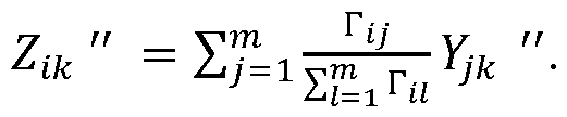 points in Y’’, using Z’’ as such might introduce a reduction in the variance, especially in the presence of entropic regularization. Therefore, in an optional step the points in Z’’ are first centred around 0, then
rescaled in such a way that they have the same as X0’’ and translated back around their original mean. This variance-based correction is an optional step in the technique of the invention. [0074] Another optional step is to re-weigh the Wasserstein distance based on which variables deserve more attention. More specifically, for each variable a p-value is derived from a two-sample unpaired statistical test. Next the expected corresponding p-values are computed, as described in a previous optional step. For each variable indexed by k, the corresponding weight uk is set to 1 when the obtained p-value is lower than its theoretical counterpart, and set to 0 otherwise. Alternatively, uk can be simply increased or decreased by a certain factor. In that latter case, the u weights are initialized to a common value (e.g., 1) before the start of the iterative loop. Finally, the weighted Wasserstein distance is defined as: ^^^^^, ^^^^ = ∑^ ^^^ ∑^ ! ^^^ Γ^^ ∑ ^^^ (^^^^^ ^^ − ^ ^ ^^ ^^^ . [0075] to prevent X’’
points in Y’’, using Z’’ as such might introduce a reduction in the variance, especially in the presence of entropic regularization. Therefore, in an optional step the points in Z’’ are first centred around 0, then
rescaled in such a way that they have the same as X0’’ and translated back around their original mean. This variance-based correction is an optional step in the technique of the invention. [0074] Another optional step is to re-weigh the Wasserstein distance based on which variables deserve more attention. More specifically, for each variable a p-value is derived from a two-sample unpaired statistical test. Next the expected corresponding p-values are computed, as described in a previous optional step. For each variable indexed by k, the corresponding weight uk is set to 1 when the obtained p-value is lower than its theoretical counterpart, and set to 0 otherwise. Alternatively, uk can be simply increased or decreased by a certain factor. In that latter case, the u weights are initialized to a common value (e.g., 1) before the start of the iterative loop. Finally, the weighted Wasserstein distance is defined as: ^^^^^, ^^^^ = ∑^ ^^^ ∑^ ! ^^^ Γ^^ ∑ ^^^ (^^^^^ ^^ − ^ ^ ^^ ^^^ . [0075] to prevent X’’
 moving too far away from the neighbourhood of X0’’. The purpose of using a regularization function here is not to induce any relaxation of the original optimal transport (OT) problem. In this sense, it differs from the well-known entropy-regularized OT described in the already mentioned paper by Courty for example. The big limitation of entropic regularization is its tendency to fill the transport plan with non-zero values, promoting barycentric mappings closer to the barycentre of the target samples, thus artificially reducing the variance originally present in the data. Such a regularization function exacerbates a phenomenon which can already be present in regular OT problems, typically in high- dimensional settings where all pairwise distances are almost equal. Preferably, chosen regularization functions should tackle these problems by designing problem-specific regularization functions. Also, the Laplacian regularization function described in the paper of Kouw only preserves the data structure but not the data itself (e.g., its position in space). Indeed, Laplacian regularization is defined by weighted pairwise squared Euclidean distances between the projected source samples, while in the approach of the present invention is instead proposed to measure dissimilarity between source samples and projected source samples. Without such design, the source samples can deviate arbitrarily far from their original position. The simplest choice for function R can be the mean squared error between X’’ and X0’’, or the mean squared error between their standardized counterparts (e.g., the mean is subtracted from each statistical variable in X’’ and X0’’, and each variable is divided by its standard deviation. Other choices are possible for R, based on the peculiarities and the nature of the data sets. [0076] The overall loss function L = W(X’’, Y’’) + λ R(X’’, X0’’) can then be computed in a differentiable manner with respect to X’, since X’’ is itself a function of X’. This results in a gradient ∇X’L of this loss function with respect to X’. All the mathematical operations described so far should be
piecewise differentiable, except the solving of plan Γ. X’ is updated using a gradient-based optimization algorithm (e.g., gradient descent, AdaGrad, Adam) using the computed ∇X’L. Because the optimal transport problem is not solved in a differentiable manner, a direct consequence is that X’ and Γ are not updated simultaneously. In that sense, the optimization procedure can be compared to a block coordinate descent algorithm. [0077] The regularisation rate λ is then decreased. In some embodiments this can be done by multiplication of the current value of λ with a certain factor (e.g., 0.9). In certain embodiments an update of λ is performed once every ω iterations with ω an integer. ω may for example be equal to 5. [0078] An alternative algorithm for correcting discrete data is now presented. As opposed to the continuous case set out above, gradient-based optimization is no longer used to update X’, and therefore, the differentiability condition on the projection function F is no longer needed. However, projection function F now should preserve the discrete nature of the data. - Data structures X and Y are obtained in different experimental conditions and comprise integer values. - Data structures X’ and Y’ are first derived from X and Y, depending on whether X and Y already lie on H or not. Since F preserves the discrete nature of the data, X’ and Y’ both contain integer values exclusively. - A vector u ∈ Rm is defined, where each component is initialized with a value of 1. uk is the probability of correcting the kth variable in any data point in the source domain. - In the iterative loop the following sub-steps are performed. First X’ is projected back on the hypersurface H using function F, whereby X’’ = F(X’) is obtained. - For each statistical variable indexed by k in the data structures X’’ and Y’’, an unpaired two- sample statistical test is performed to assess the difference between variables Xk’’ and Yk’’. Examples of such tests have been listed previously in this description. Similar to Q-Q plots, p- values are sorted in order to compute their theoretical expected value based on their ranking and on a uniformity assumption. For example, the (0.612, 0.120, 0.978, 0.789, 0.243) tuple could be assigned the expected values (0.5, 0.1, 0.9, 0.7, 0.3). The expected values can also be clipped so they are larger than a given significance threshold (e.g., 0.01). If the kth value exceeds its theoretical counterpart, then uk is decreased by a given factor (e.g., multiply it by 0.8), and vice versa. - The optimal transport problem between X’’ and Y’’ is then solved to obtain a transport plan Γ ∈ [0, 1]n×m. The transport plan is then normalized so each row sums up to one. - For each data point indexed by i in the source domain, and for each variable indexed by k, a random number ε is drawn in the [0, 1] range. If ε falls below uk, then Xik’’ is set to Yjk’’, where j
is selected at random based on the vector given by the i-th row of Γ denoted by Γi.. Otherwise, Xik’’ is set back to its initial value X0,ik’’. - If the stopping criterion is fulfilled, the iterative loop is interrupted, and the algorithm returns X’’ and Y’’ for downstream analysis. An example of stopping criterion is whether the median of previously computed p-values exceeds a given threshold (e.g., 0.5). [0079] Now the mathematical description given above is tailored to its use in a more specific method for analysing sets of nucleic acid-based count profiles. The algorithm thereby describes the protocol, the library preparation and sequencing bias removal in nucleic acid data sets such as nucleic acid sequencing data from any solid tissue or liquid cell culture or liquid/solid biopsy. More specifically, subsequent steps are described for the analysis of coverage profiles from DNA whole-genome sequencing data. Description is made for cell-free DNA, however the method remains largely applicable to genomic DNA as well. [0080] For each cell-free DNA whole-genome sequencing (WGS) sample, sequencing reads are first trimmed, then aligned to the reference genome and deduplicated. They are next aggregated into predefined bins (e.g., equal size bins of 50 kb, without being limited thereto) based on their genomic coordinates. The number of reads falling in each bin is computed for each sample, resulting in a vector of bin counts. Let n and m be the number of samples in the source and target domains, respectively. Let p also be the number of bins necessary to cover the whole genome (e.g., 56000 for the human reference genome and using bins of size 50 kb, but other values may be possible in other use cases). Read counts are stored as two matrices X ∈ ℕn×p and Y ∈ ℕm×p. For example, Xik is the number of reads spanning bin k in sample i from the source domain. Matrices X’ and Y’ are initialised by simply copying X and Y. [0081] Samples can vary in sequencing depth, therefore making X’ and Y’ non-comparable, as the sequencing depth directly influences the read counts genome-wide. The median count, computed across the sample, is used to normalise the counts and account for the differences in sequencing depths between samples. During optimization steps that are applied later, the corrected read counts matrix X’ might contain negative values, however for interpretability purposes the positivity of read counts should be enforced. Finally, the analysis of coverage profiles, as performed in the field of whole- genome sequencing data analysis, requires the read counts to be decorrelated from the GC-content of the genome. A function F is defined whose output satisfies the following constraints. (1) Given an input matrix X’, the positivity of each value is first enforced by performing Xik’ ← max(Xik’,0) for each sample i and bin k; (2) The counts of each profile are normalised by the median of the sample: Xik’ ← Xik’/medianh(Xih’);
(3) Finally, each sample is GC-corrected one of the conventional approaches (e.g., LOESS), in order to reduce the correlation between the read counts and GC-content of these bins. This commonly encountered correlation takes the form of a unimodal function. GC-content bias correction can for example be performed using Locally Weighted Scatterplot Smoothing (LOWESS), as described in “Robust Locally Weighted Regression and Smoothing Scatterplots” (Cleveland, Journal of the American Statistical Association 74 (368): 829-836, 1979). GC-content bias correction is performed the following way: Xik’ ← Xik’ / f(gk; X’,g), where f(gk; X’,g) is the smoothed estimation of Xik’ based on the GC-content of the reference genome in bin k, using a local model trained on X’ and g. The LOWESS algorithm is run on each row of the X’ matrix independently. For notational convenience, function F applies all the aforementioned sub-steps in a sequential and differentiable manner. However, since LOWESS is not a function but an algorithm itself, a description on how to compute a gradient for LOWESS is provided next. [0082] Because the presented technique is sequential and gradient-based, LOWESS should be differentiable, therefore it is required to implicitly compute the derivative of each of its outputs f(xi; y,x) with respect to yi. However, LOWESS is not a differential function but rather an iterative algorithm. Therefore, the gradient is evaluated at the final solution returned by the algorithm. In LOWESS, each data point (xi, yi) defines a local linear model, and the latter is used to predict the smoothed value +,^. Assuming the local model is linear, the latter is then expressed as ^^^ = -^^ ^., +^.^ + 0^^ ^., 1^, where αik(x,y) is the slope and βik(x,y) the intercept. One of the features of LOWESS is the weighting of data points in the regression. Let wi,j denote the weight of data point j in linear regression i. When xj is among the top f closest points to xi, this weight is given by the tricube function of |xi - xj|, and zero otherwise. The OLS (ordinary least squares) estimator of the slope is given by - ∑6 #&' 2 # ^3 # 4 3 " ^^5 # 4 5 " ^ ^^., +^ = . Let .̅^. and +,^ be the weighted the wi,. weights, respectively. The
moving too far away from the neighbourhood of X0’’. The purpose of using a regularization function here is not to induce any relaxation of the original optimal transport (OT) problem. In this sense, it differs from the well-known entropy-regularized OT described in the already mentioned paper by Courty for example. The big limitation of entropic regularization is its tendency to fill the transport plan with non-zero values, promoting barycentric mappings closer to the barycentre of the target samples, thus artificially reducing the variance originally present in the data. Such a regularization function exacerbates a phenomenon which can already be present in regular OT problems, typically in high- dimensional settings where all pairwise distances are almost equal. Preferably, chosen regularization functions should tackle these problems by designing problem-specific regularization functions. Also, the Laplacian regularization function described in the paper of Kouw only preserves the data structure but not the data itself (e.g., its position in space). Indeed, Laplacian regularization is defined by weighted pairwise squared Euclidean distances between the projected source samples, while in the approach of the present invention is instead proposed to measure dissimilarity between source samples and projected source samples. Without such design, the source samples can deviate arbitrarily far from their original position. The simplest choice for function R can be the mean squared error between X’’ and X0’’, or the mean squared error between their standardized counterparts (e.g., the mean is subtracted from each statistical variable in X’’ and X0’’, and each variable is divided by its standard deviation. Other choices are possible for R, based on the peculiarities and the nature of the data sets. [0076] The overall loss function L = W(X’’, Y’’) + λ R(X’’, X0’’) can then be computed in a differentiable manner with respect to X’, since X’’ is itself a function of X’. This results in a gradient ∇X’L of this loss function with respect to X’. All the mathematical operations described so far should be
piecewise differentiable, except the solving of plan Γ. X’ is updated using a gradient-based optimization algorithm (e.g., gradient descent, AdaGrad, Adam) using the computed ∇X’L. Because the optimal transport problem is not solved in a differentiable manner, a direct consequence is that X’ and Γ are not updated simultaneously. In that sense, the optimization procedure can be compared to a block coordinate descent algorithm. [0077] The regularisation rate λ is then decreased. In some embodiments this can be done by multiplication of the current value of λ with a certain factor (e.g., 0.9). In certain embodiments an update of λ is performed once every ω iterations with ω an integer. ω may for example be equal to 5. [0078] An alternative algorithm for correcting discrete data is now presented. As opposed to the continuous case set out above, gradient-based optimization is no longer used to update X’, and therefore, the differentiability condition on the projection function F is no longer needed. However, projection function F now should preserve the discrete nature of the data. - Data structures X and Y are obtained in different experimental conditions and comprise integer values. - Data structures X’ and Y’ are first derived from X and Y, depending on whether X and Y already lie on H or not. Since F preserves the discrete nature of the data, X’ and Y’ both contain integer values exclusively. - A vector u ∈ Rm is defined, where each component is initialized with a value of 1. uk is the probability of correcting the kth variable in any data point in the source domain. - In the iterative loop the following sub-steps are performed. First X’ is projected back on the hypersurface H using function F, whereby X’’ = F(X’) is obtained. - For each statistical variable indexed by k in the data structures X’’ and Y’’, an unpaired two- sample statistical test is performed to assess the difference between variables Xk’’ and Yk’’. Examples of such tests have been listed previously in this description. Similar to Q-Q plots, p- values are sorted in order to compute their theoretical expected value based on their ranking and on a uniformity assumption. For example, the (0.612, 0.120, 0.978, 0.789, 0.243) tuple could be assigned the expected values (0.5, 0.1, 0.9, 0.7, 0.3). The expected values can also be clipped so they are larger than a given significance threshold (e.g., 0.01). If the kth value exceeds its theoretical counterpart, then uk is decreased by a given factor (e.g., multiply it by 0.8), and vice versa. - The optimal transport problem between X’’ and Y’’ is then solved to obtain a transport plan Γ ∈ [0, 1]n×m. The transport plan is then normalized so each row sums up to one. - For each data point indexed by i in the source domain, and for each variable indexed by k, a random number ε is drawn in the [0, 1] range. If ε falls below uk, then Xik’’ is set to Yjk’’, where j
is selected at random based on the vector given by the i-th row of Γ denoted by Γi.. Otherwise, Xik’’ is set back to its initial value X0,ik’’. - If the stopping criterion is fulfilled, the iterative loop is interrupted, and the algorithm returns X’’ and Y’’ for downstream analysis. An example of stopping criterion is whether the median of previously computed p-values exceeds a given threshold (e.g., 0.5). [0079] Now the mathematical description given above is tailored to its use in a more specific method for analysing sets of nucleic acid-based count profiles. The algorithm thereby describes the protocol, the library preparation and sequencing bias removal in nucleic acid data sets such as nucleic acid sequencing data from any solid tissue or liquid cell culture or liquid/solid biopsy. More specifically, subsequent steps are described for the analysis of coverage profiles from DNA whole-genome sequencing data. Description is made for cell-free DNA, however the method remains largely applicable to genomic DNA as well. [0080] For each cell-free DNA whole-genome sequencing (WGS) sample, sequencing reads are first trimmed, then aligned to the reference genome and deduplicated. They are next aggregated into predefined bins (e.g., equal size bins of 50 kb, without being limited thereto) based on their genomic coordinates. The number of reads falling in each bin is computed for each sample, resulting in a vector of bin counts. Let n and m be the number of samples in the source and target domains, respectively. Let p also be the number of bins necessary to cover the whole genome (e.g., 56000 for the human reference genome and using bins of size 50 kb, but other values may be possible in other use cases). Read counts are stored as two matrices X ∈ ℕn×p and Y ∈ ℕm×p. For example, Xik is the number of reads spanning bin k in sample i from the source domain. Matrices X’ and Y’ are initialised by simply copying X and Y. [0081] Samples can vary in sequencing depth, therefore making X’ and Y’ non-comparable, as the sequencing depth directly influences the read counts genome-wide. The median count, computed across the sample, is used to normalise the counts and account for the differences in sequencing depths between samples. During optimization steps that are applied later, the corrected read counts matrix X’ might contain negative values, however for interpretability purposes the positivity of read counts should be enforced. Finally, the analysis of coverage profiles, as performed in the field of whole- genome sequencing data analysis, requires the read counts to be decorrelated from the GC-content of the genome. A function F is defined whose output satisfies the following constraints. (1) Given an input matrix X’, the positivity of each value is first enforced by performing Xik’ ← max(Xik’,0) for each sample i and bin k; (2) The counts of each profile are normalised by the median of the sample: Xik’ ← Xik’/medianh(Xih’);
(3) Finally, each sample is GC-corrected one of the conventional approaches (e.g., LOESS), in order to reduce the correlation between the read counts and GC-content of these bins. This commonly encountered correlation takes the form of a unimodal function. GC-content bias correction can for example be performed using Locally Weighted Scatterplot Smoothing (LOWESS), as described in “Robust Locally Weighted Regression and Smoothing Scatterplots” (Cleveland, Journal of the American Statistical Association 74 (368): 829-836, 1979). GC-content bias correction is performed the following way: Xik’ ← Xik’ / f(gk; X’,g), where f(gk; X’,g) is the smoothed estimation of Xik’ based on the GC-content of the reference genome in bin k, using a local model trained on X’ and g. The LOWESS algorithm is run on each row of the X’ matrix independently. For notational convenience, function F applies all the aforementioned sub-steps in a sequential and differentiable manner. However, since LOWESS is not a function but an algorithm itself, a description on how to compute a gradient for LOWESS is provided next. [0082] Because the presented technique is sequential and gradient-based, LOWESS should be differentiable, therefore it is required to implicitly compute the derivative of each of its outputs f(xi; y,x) with respect to yi. However, LOWESS is not a differential function but rather an iterative algorithm. Therefore, the gradient is evaluated at the final solution returned by the algorithm. In LOWESS, each data point (xi, yi) defines a local linear model, and the latter is used to predict the smoothed value +,^. Assuming the local model is linear, the latter is then expressed as ^^^ = -^^ ^., +^.^ + 0^^ ^., 1^, where αik(x,y) is the slope and βik(x,y) the intercept. One of the features of LOWESS is the weighting of data points in the regression. Let wi,j denote the weight of data point j in linear regression i. When xj is among the top f closest points to xi, this weight is given by the tricube function of |xi - xj|, and zero otherwise. The OLS (ordinary least squares) estimator of the slope is given by - ∑6 #&' 2 # ^3 # 4 3 " ^^5 # 4 5 " ^ ^^., +^ = . Let .̅^. and +,^ be the weighted the wi,. weights, respectively. The
 is then given by 0^^., +^ = +^ − -^^., +^.^. The derivative of the linear
 9 9 1 :^.^ ; +, .^ = ^.^ − .^^ -^^., +^ + = Finally, the derivative of
 > >5 " ^ ^ ^ = ^ ^ ^ - ., + ∑6 7 ? #&' 2#^3# 4 3"^ ∑ ^^^ ^^.^ − .^^ @^^ ^ − ^A ,
 where ^ ^ ^ is the Dirac delta function. The does not depend on y and is therefore the same for any profile y. As a consequence, this gradient can be precomputed at the start of the inference for efficiency purposes and at each new step multiplied with the backward gradient of each profile y. [0083] X’ represents the initial value of X’ before the iterative loop starts. The initial value of X’’ = f(X’) is stored for later use. [0084] A regularisation function R is also defined, and penalises changes in the z-scores in the source domain, as z-scores are often used in the field to detect foetal abnormalities in pregnancy, as described for example in “Systematic evaluation of NIPT aneuploidy detection software tools with clinically validated NIPT samples” (Paluoja et al, PLoS Computational Biology 17.12 (2021): e1009684). Let Sik denote the z-score for sample i and bin k, defined as Sik = (Xik’’ - μk)/σk, where μk is the mean of the kth column of X’’, and σk the standard deviation of the kth column of X’’. Let S0,ik be the z-score computed analogously based on the initial projection X0’’. The regularisation function, in its simplest form, is defined as B^^^^, ^C ^^^ = ^ ^! ∑ ^ ^^^ ∑! ^^^ ^D^^ − DC,^^^ ^ . Z-scores are used as a original data is preserved.
 [0085] The loss function, defined as the sum of the Wasserstein distance and a regularisation function is then computed in a differentiable manner. [0086] Backpropagation is used to update X’. This process is repeated until the convergence criterion is reached. The convergence criterion is defined as being satisfied when the median p-value (two-sample Kolmogorov-Smirnov test) exceeds the threshold value (e.g., 0.5). Each statistical test is performed on a particular bin and is used to assess the statistical difference between the two domains. The contribution of the regularisation to the loss function is decreased at given times, for example, every 20 iterations until the convergence criterion is satisfied. [0087] Then a new iteration of the loop is started. [0088] After the stopping criterion has been fulfilled, X’’ and Y’’ are combined into a single dataset and treated as such. If both X’’ and Y’’ contain samples from healthy donors, these samples can be grouped into a single control cohort to be used for further analysis. [0089] Optionally, the corrected profiles are validated using independent experimental methods or cross-validation techniques. This step ensures that the corrections made translate into biologically meaningful and reproducible results. For example, CNAs are called from the cfDNA read counts, and compared with known genomic alterations in a separate cohort or using orthogonal methods such as digital PCR.
[0090] Finally, the corrected cfDNA and derived insights are integrated into clinical diagnostic workflows or research protocols. For example, the corrected coverage profiles can be used for Non-Invasive Prenatal Testing (NIPT) to detect fetal aneuploidies, for monitoring cancer patients for minimal residual disease, or for studying chromosomal instability in research settings. [0091] In another application the nucleic acid is RNA, and the differences in measurement conditions is most often referred to as batch effect. After applying the algorithm, the combined data set consists of RNA-based count profiles, with alleviated batch effects. The corrected RNA-based count profiles are then used for feature extraction, pathway analysis and biomarker discovery, for example by identifying RNA signatures associated with cardiovascular diseases (e.g., atherosclerosis), neurological conditions (e.g., Alzheimer’s disease), antimicrobial resistance or cancer. Optionally, the data is next integrated into a clinical workflow for diagnostics or monitoring, such as minimal residual disease detection using cancer-specific RNA signatures, or treatment efficacy monitoring. [0092] It was already mentioned that the field of nucleic acids is only one application where a correction needs to be applied to account for a bias between two or more data sets before further analysis becomes possible. Another possible application field relates to domain adaptation for electroencephalographic (EEG) recordings. Statistical or Machine Learning models based on such data can be used to detect epileptic seizures, diagnose sleep disorders, help in the context of biofeedback therapy, neurorehabilitation or be part of the design of brain-computer interfaces (prostheses, assistive devices for people with communicative disabilities). [0093] EEG recordings are obtained from e (e.g., 32) electrodes, in (at least) two different experimental settings (e.g., different patient, same patient during different sessions or using different equipment), referred to as the source and target domains. [0094] Again it is first explained how the algorithm presented above in general is fine-tuned for use in this specific context. [0095] An epoch segmentation is performed on the recordings. Each time series from each recording is divided into small time segments based on fixed time intervals or specific events. The first and second data sets, from the source and target domains, respectively, are segmented into n and m time segments, respectively. These time windows are allowed to overlap (e.g., typically by half a window). [0096] The sample covariance matrices are computed in the source domain and concatenated into a single tensor ^ ∈ ℝ^×G×G, where n is the number of time segments (all recordings/patients combined) and e electrodes. ^ is the covariance between electrodes a and b for time
[0085] The loss function, defined as the sum of the Wasserstein distance and a regularisation function is then computed in a differentiable manner. [0086] Backpropagation is used to update X’. This process is repeated until the convergence criterion is reached. The convergence criterion is defined as being satisfied when the median p-value (two-sample Kolmogorov-Smirnov test) exceeds the threshold value (e.g., 0.5). Each statistical test is performed on a particular bin and is used to assess the statistical difference between the two domains. The contribution of the regularisation to the loss function is decreased at given times, for example, every 20 iterations until the convergence criterion is satisfied. [0087] Then a new iteration of the loop is started. [0088] After the stopping criterion has been fulfilled, X’’ and Y’’ are combined into a single dataset and treated as such. If both X’’ and Y’’ contain samples from healthy donors, these samples can be grouped into a single control cohort to be used for further analysis. [0089] Optionally, the corrected profiles are validated using independent experimental methods or cross-validation techniques. This step ensures that the corrections made translate into biologically meaningful and reproducible results. For example, CNAs are called from the cfDNA read counts, and compared with known genomic alterations in a separate cohort or using orthogonal methods such as digital PCR.
[0090] Finally, the corrected cfDNA and derived insights are integrated into clinical diagnostic workflows or research protocols. For example, the corrected coverage profiles can be used for Non-Invasive Prenatal Testing (NIPT) to detect fetal aneuploidies, for monitoring cancer patients for minimal residual disease, or for studying chromosomal instability in research settings. [0091] In another application the nucleic acid is RNA, and the differences in measurement conditions is most often referred to as batch effect. After applying the algorithm, the combined data set consists of RNA-based count profiles, with alleviated batch effects. The corrected RNA-based count profiles are then used for feature extraction, pathway analysis and biomarker discovery, for example by identifying RNA signatures associated with cardiovascular diseases (e.g., atherosclerosis), neurological conditions (e.g., Alzheimer’s disease), antimicrobial resistance or cancer. Optionally, the data is next integrated into a clinical workflow for diagnostics or monitoring, such as minimal residual disease detection using cancer-specific RNA signatures, or treatment efficacy monitoring. [0092] It was already mentioned that the field of nucleic acids is only one application where a correction needs to be applied to account for a bias between two or more data sets before further analysis becomes possible. Another possible application field relates to domain adaptation for electroencephalographic (EEG) recordings. Statistical or Machine Learning models based on such data can be used to detect epileptic seizures, diagnose sleep disorders, help in the context of biofeedback therapy, neurorehabilitation or be part of the design of brain-computer interfaces (prostheses, assistive devices for people with communicative disabilities). [0093] EEG recordings are obtained from e (e.g., 32) electrodes, in (at least) two different experimental settings (e.g., different patient, same patient during different sessions or using different equipment), referred to as the source and target domains. [0094] Again it is first explained how the algorithm presented above in general is fine-tuned for use in this specific context. [0095] An epoch segmentation is performed on the recordings. Each time series from each recording is divided into small time segments based on fixed time intervals or specific events. The first and second data sets, from the source and target domains, respectively, are segmented into n and m time segments, respectively. These time windows are allowed to overlap (e.g., typically by half a window). [0096] The sample covariance matrices are computed in the source domain and concatenated into a single tensor ^ ∈ ℝ^×G×G, where n is the number of time segments (all recordings/patients combined) and e electrodes. ^ is the covariance between electrodes a and b for time
 ^HI segment i. The covariance matrices ^ ∈ ℝ^×G×G in the target domain are computed similarly.
[0097] The mean J ∈ ℝG×G of all matrices is computed in both source and target domains. While computing the Euclidean mean of the matrices is a viable option, the Riemannian mean may be more informative as it accounts for the geometry of positive-definite matrices. In the present case, the Riemannian mean P is the symmetric positive-definite matrix that minimises the sum of Euclidean distances ∑^ ^^^ ^K ^J, ^^ ^^^ + ∑^ ^^^ ^K^J, ^^ ^^^ . A closed form for such a analysis on symmetric spaces:
^HI segment i. The covariance matrices ^ ∈ ℝ^×G×G in the target domain are computed similarly.
[0097] The mean J ∈ ℝG×G of all matrices is computed in both source and target domains. While computing the Euclidean mean of the matrices is a viable option, the Riemannian mean may be more informative as it accounts for the geometry of positive-definite matrices. In the present case, the Riemannian mean P is the symmetric positive-definite matrix that minimises the sum of Euclidean distances ∑^ ^^^ ^K ^J, ^^ ^^^ + ∑^ ^^^ ^K^J, ^^ ^^^ . A closed form for such a analysis on symmetric spaces:
 Statistics of diffusion tensors” (Fletcher and Sarang, Int’l Workshop on Mathematical Methods in Medical and Biomedical Image Analysis, Berlin, 2004), the Riemannian mean is found using an iterative algorithm wherein repeatedly the exponential mapping of the average of the logarithmic mappings of all matrices is taken. Exponential and logarithmic mappings are described in the next step. [0098] Covariance matrices are matrices with a specific structure and relationship between their elements, as they are symmetric positive-definite, and they are part of a Riemannian manifold. Given a tangent point P, the logarithmic mapping X’ = LogP(X’’) maps covariance matrix X’ to the tangent space defined by P, and the exponential mapping X’’ = ExpP(X’) maps X’ back on the manifold. Connecting to the description of the most generic form applied in the method of the invention, F(X’) is defined as the function that performs the exponential mapping ExpP(X’) on each matrix X located on the tangent space at P. Before correcting data in the source domain, the inverse function X’ = F(X) is first applied, as it is planned to freely optimise X’ in the Euclidean space. [0099] L ∈ ℝ^×^ is computed, where L^^ = ^N^^^ ∗^, ^^ ∗^^ is the Riemannian distance between covariance matrices Xi’ and Xj’. The Riemannian metric ^N is defined in “Multiclass brain- computer interface classification by Riemannian geometry” (Barachant et al., IEEE Trans. on Biomedical Engineering, 59.4 (2011): 920-928) as ^N^J^, J^^ = |log^J^ 4^J^^|S = T∑G ^^^ log^ U^ . [0100] A regularisation rate λ is arbitrarily chosen, for example a high value like 1e+4. [0101] Then the iterative loop is started, which is repeated until convergence is reached. First X’ is projected on the tangent plane at P and then back on the manifold using F to obtain X’’ = F(X’). [0102] For each electrode pair (a, b), a two-sample statistical test (e.g., Kolmogorov-Smirnov) is performed to assess the difference between X.ab’ and Y.ab’. This results in a set of e² p-values. If the median value of this set exceeds a predetermined threshold (e.g., 0.5), the iterative loop stops here. [0103] The optimal transport problem between X’’ and Y’’ to obtain a transport plan Γ is solved whereby the Wasserstein distance is computed, as already described previously. [0104] The regularisation function is then computed as
. [0105] After backpropagation X’ is updated using any gradient-based optimization algorithm. [0106] The regularization rate λ is adapted, for example decreased with a given factor (e.g. multiplied with 0.9). Then a next iteration of the loop can be performed. [0107] After the convergence criterion is fulfilled, data tensors X’’ and Y’’ are combined into a single dataset and treated as such, despite X and Y having originally been collected from different subjects or in different experimental settings. [0108] Optionally, corrected data is validated using independent experimental methods or cross-validation techniques. This step ensures that the corrections made led to biologically meaningful and reproducible results. For instance, the corrected EEG features can be compared with known biomarkers or replicated in a different cohort of subjects. [0109] Finally, the corrected EEG data and derived insights are integrated into clinical diagnostics workflows or research protocols. The applications of covariance matrices derived from EEG recordings are plentiful. Statistical or Machine Learning models based on such data can be used for the early diagnosis of neurological disorders, sleep disorders, treatment efficacy monitoring, biofeedback therapy or neurorehabilitation. In research settings, they can be used as part of the study of cognitive processes or for the design of brain-computer interfaces (prostheses, assistive devices for people with communicative disabilities). [0110] While the invention has been illustrated and described in detail in the drawings and foregoing description, such illustration and description are to be considered illustrative or exemplary and not restrictive. The foregoing description details certain embodiments of the invention. It will be appreciated, however, that no matter how detailed the foregoing appears in text, the invention may be practiced in many ways. The invention is not limited to the disclosed embodiments. [0111] Other variations to the disclosed embodiments can be understood and effected by those skilled in the art in practicing the claimed invention, from a study of the drawings, the disclosure and the appended claims. In the claims, the word “comprising” does not exclude other elements or steps, and the indefinite article “a” or “an” does not exclude a plurality. A single processor or other unit may fulfil the functions of several items recited in the claims. The mere fact that certain measures are recited in mutually different dependent claims does not indicate that a combination of these measures cannot be used to advantage. A computer program may be stored/distributed on a suitable medium, such as an optical storage medium or a solid-state medium supplied together with or as part of other hardware, but may also be distributed in other forms, such as via the Internet or other wired or wireless
telecommunication systems. Any reference the claims should not be construed as limiting the scope.
Statistics of diffusion tensors” (Fletcher and Sarang, Int’l Workshop on Mathematical Methods in Medical and Biomedical Image Analysis, Berlin, 2004), the Riemannian mean is found using an iterative algorithm wherein repeatedly the exponential mapping of the average of the logarithmic mappings of all matrices is taken. Exponential and logarithmic mappings are described in the next step. [0098] Covariance matrices are matrices with a specific structure and relationship between their elements, as they are symmetric positive-definite, and they are part of a Riemannian manifold. Given a tangent point P, the logarithmic mapping X’ = LogP(X’’) maps covariance matrix X’ to the tangent space defined by P, and the exponential mapping X’’ = ExpP(X’) maps X’ back on the manifold. Connecting to the description of the most generic form applied in the method of the invention, F(X’) is defined as the function that performs the exponential mapping ExpP(X’) on each matrix X located on the tangent space at P. Before correcting data in the source domain, the inverse function X’ = F(X) is first applied, as it is planned to freely optimise X’ in the Euclidean space. [0099] L ∈ ℝ^×^ is computed, where L^^ = ^N^^^ ∗^, ^^ ∗^^ is the Riemannian distance between covariance matrices Xi’ and Xj’. The Riemannian metric ^N is defined in “Multiclass brain- computer interface classification by Riemannian geometry” (Barachant et al., IEEE Trans. on Biomedical Engineering, 59.4 (2011): 920-928) as ^N^J^, J^^ = |log^J^ 4^J^^|S = T∑G ^^^ log^ U^ . [0100] A regularisation rate λ is arbitrarily chosen, for example a high value like 1e+4. [0101] Then the iterative loop is started, which is repeated until convergence is reached. First X’ is projected on the tangent plane at P and then back on the manifold using F to obtain X’’ = F(X’). [0102] For each electrode pair (a, b), a two-sample statistical test (e.g., Kolmogorov-Smirnov) is performed to assess the difference between X.ab’ and Y.ab’. This results in a set of e² p-values. If the median value of this set exceeds a predetermined threshold (e.g., 0.5), the iterative loop stops here. [0103] The optimal transport problem between X’’ and Y’’ to obtain a transport plan Γ is solved whereby the Wasserstein distance is computed, as already described previously. [0104] The regularisation function is then computed as
. [0105] After backpropagation X’ is updated using any gradient-based optimization algorithm. [0106] The regularization rate λ is adapted, for example decreased with a given factor (e.g. multiplied with 0.9). Then a next iteration of the loop can be performed. [0107] After the convergence criterion is fulfilled, data tensors X’’ and Y’’ are combined into a single dataset and treated as such, despite X and Y having originally been collected from different subjects or in different experimental settings. [0108] Optionally, corrected data is validated using independent experimental methods or cross-validation techniques. This step ensures that the corrections made led to biologically meaningful and reproducible results. For instance, the corrected EEG features can be compared with known biomarkers or replicated in a different cohort of subjects. [0109] Finally, the corrected EEG data and derived insights are integrated into clinical diagnostics workflows or research protocols. The applications of covariance matrices derived from EEG recordings are plentiful. Statistical or Machine Learning models based on such data can be used for the early diagnosis of neurological disorders, sleep disorders, treatment efficacy monitoring, biofeedback therapy or neurorehabilitation. In research settings, they can be used as part of the study of cognitive processes or for the design of brain-computer interfaces (prostheses, assistive devices for people with communicative disabilities). [0110] While the invention has been illustrated and described in detail in the drawings and foregoing description, such illustration and description are to be considered illustrative or exemplary and not restrictive. The foregoing description details certain embodiments of the invention. It will be appreciated, however, that no matter how detailed the foregoing appears in text, the invention may be practiced in many ways. The invention is not limited to the disclosed embodiments. [0111] Other variations to the disclosed embodiments can be understood and effected by those skilled in the art in practicing the claimed invention, from a study of the drawings, the disclosure and the appended claims. In the claims, the word “comprising” does not exclude other elements or steps, and the indefinite article “a” or “an” does not exclude a plurality. A single processor or other unit may fulfil the functions of several items recited in the claims. The mere fact that certain measures are recited in mutually different dependent claims does not indicate that a combination of these measures cannot be used to advantage. A computer program may be stored/distributed on a suitable medium, such as an optical storage medium or a solid-state medium supplied together with or as part of other hardware, but may also be distributed in other forms, such as via the Internet or other wired or wireless
telecommunication systems. Any reference the claims should not be construed as limiting the scope.
Claims
Claims 1. Computer-implemented method for analysing data obtained by combining a first set (X) of nucleic acid-based count profiles with a second set (Y) of nucleic acid-based count profiles, said second set being obtained in different measurement conditions than said first set, the method comprising: - defining a regularisation function to preserve properties of said first set of nucleic acid-based count profiles, - initialising a data structure, X’, derived from said first set of nucleic acid-based count profiles, - determining a projection, Y’’, of a data structure derived from said second set of nucleic acid-based count profiles on a hypersurface using a function F imposing one or more constraints on the data in said data structure derived from said second set of nucleic acid-based count profiles, - taking an initial value for a regularisation rate, - performing the following substeps: - determining a projection, X’’, of data comprised in said data structure, X’, on said hypersurface using said function, - performing statistical testing to assess differences between the projected data X’’ of said data structure and said projection Y’, said statistical testing yielding a plurality of values indicative of a similarity between statistical distributions of X’’ and Y’, - finding a solution of an optimal transport problem between X’’ and Y’, so obtaining a transport plan between data points of X’’ and data points of Y’, - computing said regularisation function for said projection X’’, - computing a loss function derived from said solution of said optimal transport problem, said computed regularisation function and said regularisation rate, - updating said data structure, X’, using a gradient of said loss function with respect to X’, until a reference value obtained from said plurality of values indicative of said similarity reaches a predetermined threshold, and thus a combination of said first set and said second set is obtained wherein bias caused by said different measurement conditions is reduced.
2. Computer-implemented method as in claim 1, comprising a step of adapting said regularisation rate.
3. Computer-implemented method as in claim 2, wherein said adapting is performed once every M iterations, M being an integer.
4. Computer-implemented method as in any of claims 1 to 3, wherein said statistical testing comprises performing an unpaired two-sample statistical test.
5. Computer-implemented method as in any of the previous claims, wherein the optimal transport problem is expressed as a regression problem with variance-based corrected target values.
6. Computer-implemented method as in any of previous claims, wherein at least one variable in the optimal transport problem is given a different weight compared to other variables in the optimal transport problem.
7. Computer-implemented method as in any of the previous claims, comprising a step of using the resulting projection X’’ for further analysis.
8. Computer-implemented method as in any of the previous claims, wherein a plurality of first sets is combined with said second set, each first set of said plurality being obtained in different measurement conditions.
9. Computer-implemented method as in any of the previous claims, wherein said nucleic acid is DNA.
10. Computer-implemented method as in claim 9, wherein said DNA is generated from solid tissues and/or liquid cell cultures and/or liquid biopsies.
11. Computer-implemented method as in claim 9 or 10, wherein said DNA is cell-free DNA.
12. Computer-implemented method as in any of claims 9 to 11, comprising a step of performing copy number aberration analysis on count profiles from said combination of said first set and said second set.
13. Computer-implemented method as in any of claims 1 to 8, wherein said nucleic acid is RNA.
14. Computer-implemented method as in claim 13, comprising performing on said combination of said first set and said second set a step of at least one of {feature extraction, pathway analysis, biomarker discovery}.
Applications Claiming Priority (4)
| Application Number | Priority Date | Filing Date | Title |
|---|---|---|---|
| EP23178519.7 | 2023-06-09 | ||
| EP23178519 | 2023-06-09 | ||
| EP23213255.5 | 2023-11-30 | ||
| EP23213255 | 2023-11-30 |
Publications (1)
| Publication Number | Publication Date |
|---|---|
| WO2024252025A1 true WO2024252025A1 (en) | 2024-12-12 |
Family
ID=91431564
Family Applications (1)
| Application Number | Title | Priority Date | Filing Date |
|---|---|---|---|
| PCT/EP2024/065927 Ceased WO2024252025A1 (en) | 2023-06-09 | 2024-06-10 | Method for analysing data from different measurement conditions |
Country Status (1)
| Country | Link |
|---|---|
| WO (1) | WO2024252025A1 (en) |
Cited By (1)
| Publication number | Priority date | Publication date | Assignee | Title |
|---|---|---|---|---|
| CN120258457A (en) * | 2025-04-03 | 2025-07-04 | 国网上海市电力公司 | Dynamic aggregation and optimization scheduling method and system for urban regional integrated energy system |
-
2024
- 2024-06-10 WO PCT/EP2024/065927 patent/WO2024252025A1/en not_active Ceased
Non-Patent Citations (13)
| Title |
|---|
| BARACHANT ET AL., IEEE TRANS. ON BIOMEDICAL ENGINEERING, vol. 59, no. 4, 2011, pages 920 - 928 |
| CHE ET AL., NPJ GENOMIC MEDICINE, vol. 7, no. 1, 2022, pages 55 |
| CLEVELAND, JOURNAL OF THE AMERICAN STATISTICAL ASSOCIATION, vol. 74, no. 368, 1979, pages 829 - 836 |
| DUCHI ET AL., JOURNAL OF MACHINE LEARNING RESEARCH, vol. 12, no. 7, 2011 |
| JU ET AL.: "Annual Int'I Conf", IEEE ENG. IN MEDICINE & BIOLOGY SOC, 2020 |
| LIANG ET AL., FRONTIERS IN HUMAN NEUROSCIENCE, 2022 |
| N. COURTY ET AL., IEEE TRANS. PATTERN ANALYSIS AND MACHINE INTELLIGENCE, vol. 39, no. 9, 22 June 2016 (2016-06-22), pages 1853 - 1865 |
| NICOLAS COURTY: "Optimal Transport for Domain Adaptation", vol. 39, no. 9, 22 June 2016 (2016-06-22), USA, pages 1853 - 1865, XP093156045, ISSN: 0162-8828, Retrieved from the Internet <URL:https://arxiv.org/pdf/1507.00504> [retrieved on 20240425], DOI: 10.1109/TPAMI.2016.2615921 * |
| PALUOJA ET AL., PLOS COMPUTATIONAL BIOLOGY, vol. 17, no. 12, 2021, pages e1009684 |
| SCHWEIKERT ET AL., ADVANCES IN NEURAL INFORMATION PROCESSING SYSTEMS, 2009, pages 1433 - 1440 |
| SHENGJIN LIANG: "Multi-source joint domain adaptation for cross-subject and cross-session emotion recognition from electroencephalography", FRONTIERS IN HUMAN NEUROSCIENCE, vol. 16, 15 September 2022 (2022-09-15), CH, XP093156147, ISSN: 1662-5161, DOI: 10.3389/fnhum.2022.921346 * |
| W. KOUW ET AL.: "Library", 24 July 2019, CORNELL UNIVERSITY |
| WOUTER M KOUW ET AL: "A review of domain adaptation without target labels", ARXIV.ORG, CORNELL UNIVERSITY LIBRARY, 201 OLIN LIBRARY CORNELL UNIVERSITY ITHACA, NY 14853, 24 July 2019 (2019-07-24), XP081933113, DOI: 10.1109/TPAMI.2019.2945942 * |
Cited By (1)
| Publication number | Priority date | Publication date | Assignee | Title |
|---|---|---|---|---|
| CN120258457A (en) * | 2025-04-03 | 2025-07-04 | 国网上海市电力公司 | Dynamic aggregation and optimization scheduling method and system for urban regional integrated energy system |
Similar Documents
| Publication | Publication Date | Title |
|---|---|---|
| Albahra et al. | Artificial intelligence and machine learning overview in pathology & laboratory medicine: A general review of data preprocessing and basic supervised concepts | |
| Barzekar et al. | C-Net: A reliable convolutional neural network for biomedical image classification | |
| CN111933212B (en) | A machine learning-based clinical omics data processing method and device | |
| US12260939B2 (en) | Systems and methods for predicting compounds associated with transcriptional signatures | |
| Sun et al. | Local-learning-based feature selection for high-dimensional data analysis | |
| Huang et al. | From quantitative microscopy to automated image understanding | |
| JP2023501126A (en) | Multi-instance learner for tissue image classification | |
| Lee et al. | Classification of bioinformatics dataset using finite impulse response extreme learning machine for cancer diagnosis | |
| Billah et al. | Bayesian convolutional neural network-based models for diagnosis of blood cancer | |
| US20240112803A1 (en) | Systems and Methods for Dynamic Raman Profiling of Biological Diseases and Disorders | |
| EP4537088A1 (en) | Systems and methods for dynamic raman profiling of biological diseases and disorders and feature engineering methods thereof | |
| US20140309122A1 (en) | Knowledge-driven sparse learning approach to identifying interpretable high-order feature interactions for system output prediction | |
| CN115116551B (en) | A method for predicting protein interaction relationships based on non-negative matrix factorization framework | |
| Tran et al. | Un-normalized graph p-Laplacian semi-supervised learning method applied to cancer classification problem | |
| EP4531057A1 (en) | Methods and systems for disease phenotyping using multimodal ehr data and weak supervision | |
| Lerner et al. | On the classification of a small imbalanced cytogenetic image database | |
| Ragunthar et al. | Classification of gene expression data with optimized feature selection | |
| Wang et al. | Using artificial intelligence to interpret clinical flow cytometry datasets for automated disease diagnosis and/or monitoring | |
| Sankaranarayanan et al. | Optimized twin spatio-temporal convolutional neural network with squeezenet transfer learning model for cancer miRNA biomarker classification | |
| Praveena et al. | Chromosome Image Classification Using Edge Fusion Attention Network | |
| Wang et al. | Signal subgraph estimation via vertex screening | |
| Jagetiya et al. | Optimizing breast cancer prognosis with machine learning for enhanced clinical decision-making | |
| Di Caro et al. | Quantum Cognition Machine Learning for Forecasting Chromosomal Instability | |
| Rodrigues et al. | Deterministic classifiers accuracy optimization for cancer microarray data | |
| CN107710206B (en) | Methods, systems and devices for subpopulation detection from biological data |
Legal Events
| Date | Code | Title | Description |
|---|---|---|---|
| 121 | Ep: the epo has been informed by wipo that ep was designated in this application |
Ref document number: 24731374 Country of ref document: EP Kind code of ref document: A1 |
|
| DPE1 | Request for preliminary examination filed after expiration of 19th month from priority date (pct application filed from 20040101) | ||
| NENP | Non-entry into the national phase |
Ref country code: DE |
|
| 122 | Ep: pct application non-entry in european phase |
Ref document number: 24731374 Country of ref document: EP Kind code of ref document: A1 |