WO2024057299A1 - Probes, apparatuses and methods for use in scanning probe microscopy - Google Patents
Probes, apparatuses and methods for use in scanning probe microscopy Download PDFInfo
- Publication number
- WO2024057299A1 WO2024057299A1 PCT/IL2023/050201 IL2023050201W WO2024057299A1 WO 2024057299 A1 WO2024057299 A1 WO 2024057299A1 IL 2023050201 W IL2023050201 W IL 2023050201W WO 2024057299 A1 WO2024057299 A1 WO 2024057299A1
- Authority
- WO
- WIPO (PCT)
- Prior art keywords
- probe
- layer
- sample
- tunneling
- stage
- Prior art date
- Legal status (The legal status is an assumption and is not a legal conclusion. Google has not performed a legal analysis and makes no representation as to the accuracy of the status listed.)
- Ceased
Links
Classifications
-
- G—PHYSICS
- G01—MEASURING; TESTING
- G01Q—SCANNING-PROBE TECHNIQUES OR APPARATUS; APPLICATIONS OF SCANNING-PROBE TECHNIQUES, e.g. SCANNING PROBE MICROSCOPY [SPM]
- G01Q70/00—General aspects of SPM probes, their manufacture or their related instrumentation, insofar as they are not specially adapted to a single SPM technique covered by group G01Q60/00
- G01Q70/08—Probe characteristics
- G01Q70/14—Particular materials
-
- G—PHYSICS
- G01—MEASURING; TESTING
- G01Q—SCANNING-PROBE TECHNIQUES OR APPARATUS; APPLICATIONS OF SCANNING-PROBE TECHNIQUES, e.g. SCANNING PROBE MICROSCOPY [SPM]
- G01Q10/00—Scanning or positioning arrangements, i.e. arrangements for actively controlling the movement or position of the probe
- G01Q10/02—Coarse scanning or positioning
-
- G—PHYSICS
- G01—MEASURING; TESTING
- G01Q—SCANNING-PROBE TECHNIQUES OR APPARATUS; APPLICATIONS OF SCANNING-PROBE TECHNIQUES, e.g. SCANNING PROBE MICROSCOPY [SPM]
- G01Q10/00—Scanning or positioning arrangements, i.e. arrangements for actively controlling the movement or position of the probe
- G01Q10/04—Fine scanning or positioning
-
- G—PHYSICS
- G01—MEASURING; TESTING
- G01Q—SCANNING-PROBE TECHNIQUES OR APPARATUS; APPLICATIONS OF SCANNING-PROBE TECHNIQUES, e.g. SCANNING PROBE MICROSCOPY [SPM]
- G01Q60/00—Particular types of SPM [Scanning Probe Microscopy] or microscopes; Essential components thereof
- G01Q60/10—STM [Scanning Tunnelling Microscopy] or apparatus therefor, e.g. STM probes
- G01Q60/16—Probes, their manufacture, or their related instrumentation, e.g. holders
-
- G—PHYSICS
- G01—MEASURING; TESTING
- G01Q—SCANNING-PROBE TECHNIQUES OR APPARATUS; APPLICATIONS OF SCANNING-PROBE TECHNIQUES, e.g. SCANNING PROBE MICROSCOPY [SPM]
- G01Q60/00—Particular types of SPM [Scanning Probe Microscopy] or microscopes; Essential components thereof
- G01Q60/24—AFM [Atomic Force Microscopy] or apparatus therefor, e.g. AFM probes
- G01Q60/38—Probes, their manufacture, or their related instrumentation, e.g. holders
- G01Q60/40—Conductive probes
-
- G—PHYSICS
- G01—MEASURING; TESTING
- G01Q—SCANNING-PROBE TECHNIQUES OR APPARATUS; APPLICATIONS OF SCANNING-PROBE TECHNIQUES, e.g. SCANNING PROBE MICROSCOPY [SPM]
- G01Q70/00—General aspects of SPM probes, their manufacture or their related instrumentation, insofar as they are not specially adapted to a single SPM technique covered by group G01Q60/00
- G01Q70/08—Probe characteristics
- G01Q70/10—Shape or taper
-
- G—PHYSICS
- G01—MEASURING; TESTING
- G01Q—SCANNING-PROBE TECHNIQUES OR APPARATUS; APPLICATIONS OF SCANNING-PROBE TECHNIQUES, e.g. SCANNING PROBE MICROSCOPY [SPM]
- G01Q60/00—Particular types of SPM [Scanning Probe Microscopy] or microscopes; Essential components thereof
- G01Q60/24—AFM [Atomic Force Microscopy] or apparatus therefor, e.g. AFM probes
- G01Q60/36—DC mode
- G01Q60/363—Contact-mode AFM
Definitions
- This disclosure relates to the field of scanning probe microscopy (SPM).
- Scanning probe microscopy is a branch of microscopy that forms images of the mechanical and electronic properties of surfaces using a physical probe that scans across the sample. It includes such types as atomic force microscopy (AFM), scanning tunneling microscopy (STM), and others.
- AFM includes such a sub-type as conductive AFM (CAFM, C-AFM) or current sensing AFM (CS-AFM).
- CAFM conductive AFM
- C-AFM current sensing AFM
- Other names for such techniques, or related techniques are local-conductivity AFM (LC-AFM), conductive probe AFM (CP-AFM), conductive scanning probe microscopy (C-SPM) or conductive scanning force microscopy (C-SFM).
- CAFM uses a sharp conductive probe to map local variations in a sample’s conductivity with nanoscale resolution. It is used to study a sample’s conductivity and image electrical properties such as charge transport and charge distribution on the nanoscale.
- CAFM is applied in the nanoelectronics field, solar cell and semiconductor industries for a wide variety of high resolution measurements including semiconductor dopant profiling and quality control for dielectric films and oxide layers.
- the conducting probe in CAFM typically has a thin conducting coating.
- Common electrically conducting coatings are platinum, gold, tungsten, and conductive diamond.
- CAFM is usually operated in contact mode: a bias voltage is applied between AFM tip and sample when they are in contact, and the current flow is measured between them as the probe raster scans across the surface.
- the contact area between tip and sample typically has a diameter in the 10 nm range.
- the topography of the surface is measured by detecting the deflection of the cantilever where the tip resides using an optical system (for example, a laser combined with a photodiode) or using a piezoresistive technique.
- I- V current- voltage
- CAFM CAFM
- the scanning contact mode of operation can lead to an aggressive tipsample interaction that can wear down the tip quickly.
- surface contamination and a water film between tip and sample commonly present at ambient conditions, can reduce the reliability and repeatability of CAFM.
- Only a few nanometers of debris on the tip can block the flow of electrical current. Consequently, as mentioned in Ref. 2, higher forces are often needed, requiring harder tip materials or coatings like conductive diamond-like coatings or platinum silicide since these higher forces will degrade the tip faster.
- the inventors have found techniques which can be used in contact mode to obtain the current measurements.
- the technique of the present disclosure is not limited to be implemented in CAFM; but rather can be used in systems which differ from CAFM in the structures of the probe; and/or in the type of the measured current or specifics of the characterization which it brings about; and/or in samples at which these techniques are primarily aimed; and/or in the setup and method realizing the scanning in the contact mode.
- the inventors have termed the relevant techniques/systems as Quantum Twisting Microscopy.
- the probes suitable for use in the scanning techniques of the present disclosure are characterized by such features as a tip having a core with an apex, where this apex is covered by an active layer presenting a two-dimensional (2D) material of not more than 10 monolayers coupled by van der Waals (vdW) forces, and the active layer is placed on a support layer of a vdW material: the active layer at that apex is thereby further away from the core than the support layer at that apex (and the active and support layers form a vdW heterostructure at the apex).
- 2D two-dimensional
- the probes utilized in the technique of the present disclosure share the feature of a layer arrangement, covering the apex and the core of the tip and including at the apex at least the support layer and the active layer, which is configured to form, under a pressure against a planar surface, a contact area containing a square with a side of 10 nm or more.
- the contact area may take various geometrical shapes, but it contains a square with a side of 10 nm or more.
- the flat or flattened contact area may be larger or smaller than the apex area.
- An outer layer of the layer arrangement (by which it faces the sample) is an exposed layer.
- the probes utilized in the technique of the present disclosure share the feature that the layer arrangement is configured to conduct an electric current to the active layer from outside (i.e. from an exposed layer if this is not the active layer, but a more externally placed layer) and then, at the apex, in a lateral dimension (substantially or even only) and through the active layer (substantially or only).
- the active layer at the apex is the exposed layer.
- the tip at the apex is further covered by a tunnel barrier layer placed on the active layer; and it is the tunnel barrier layer which is the exposed layer.
- This tunnel barrier layer is thereby configured to present a flow path for a tunneling current between the sample and the 2D material of the active layer.
- the tip at the apex is covered instead by a defect- assisted tunneling layer on the active layer (i.e., instead of the tunnel barrier layer).
- the defect-assisted tunneling layer is the exposed layer and includes at least one atomic defect which presents a tunneling path for tunneling between the sample and the active layer.
- Each such atomic defect may provide a peak of tunneling conductance at a certain unique voltage between (a) a region proximate to the defect on the active layer and (b) a region proximate to the defect and located beyond the exposed defect-assisted tunneling layer.
- the sample is to be placed into the latter region.
- the term “unique voltage” is used meaning that voltages are expected to differ for different defects).
- the layer arrangement which at the apex additionally includes the defect-assisted tunneling layer, conducts the electric current by at least the tunneling via the at least one atomic defect in this layer when the applied voltage allows it (and then in a lateral dimension and through the active layer).
- the core presents the bulk of the tip and it may be made of a conductive material, such as a metal or a semiconductor or an alloy (e.g., Tungsten, Platinum, Platinum-Iridium, doped silicon, etc.); or of a dielectric (e.g., silicon, quartz, sapphire, diamond, etc.).
- a conductive material such as a metal or a semiconductor or an alloy (e.g., Tungsten, Platinum, Platinum-Iridium, doped silicon, etc.); or of a dielectric (e.g., silicon, quartz, sapphire, diamond, etc.).
- a dielectric material a material with the bandgap larger than 2 eV is meant; and by the semiconductor, a material with non-zero bandgap smaller than 2 eV is meant.
- the core may have a length larger than 1 micron (pm); and/or smaller than 10 mm (lengths closer to this value may correspond to cores which are similar to STM tips). In some of the experiments conducted by the inventors, the length was in a range 1.2- 1.6 pm.
- 2D materials are substances with a thickness of a few nanometers, which are characterized by a layered crystal structure with strong bonds - covalent or ionic - within each layer, and where layers are coupled together by relatively weak vdW forces.
- insulators band insulators, topological insulators, and Mott insulators.
- the carriers for example, electrons
- the 2D material may have not more than any smaller number of monolayers instead of 10: for example, the upper limit for the number of monolayers may be 7, or 4, 3, 2, or 1).
- the monolayers may differ in chemical composition, and the 2D material forming the active layer may be itself formed from monolayers of different 2D materials when they couple by vdW forces.
- suitable 2D material for the active layer examples include the semimetal graphene, transition metal dichalcogenides (TMDs) semiconductors including but not limited to WSe2, WS2, MoSe2, M0S2, TaSe2, TaS2, NbSe2, WTe2 and so forth, RuCh or similar 2D magnetic layers, BiSCCO or similar layered high- superconductingtemperature materials.
- TMDs transition metal dichalcogenides
- the support layer carrying at the apex the active layer is made of a vdW material.
- the support layer allows for the active layer to have the proper functionality: the active layer has to be sufficiently thin to be 2D, but if it was placed directly on the apex of the tip’s core of some conventional material, it would bend and strain and thus loose its desired mechanical and/or electrical properties, since the apex could be too rugged.
- the support layer is selected to mitigate or prevent the chance that the vdW material of the active layer would not form the appropriately conducting and mechanically suitable for use in the probe 2D vdW material.
- the support layer does not have to be a 2D material. It will have more than 10 monolayers. It can be a dielectric, or a semiconductor, or even a conductor, such as semimetal or a metal if an interface between the active layer and the support layer has a very small probability for a carrier to get transmitted therethrough upon one impinging on the interface. The latter can happen, for example, in case of a mismatch between lattices of the active layer and the support layer, or different orientations if they are made of the same material, resulting for example in a contact resistance greatly suppressing the current.
- the contact resistance higher than 10 times Sharvin resistance between the active layer and the support layer is suitable (a skilled person would readily find this resistance; but in any case, the formula for the ballistic case, which can serve as a reference, for different contact interfaces was originally presented in Sharvin, Yu. V. “;4 possible method for studying Fermi surfaces Sov. Phys. JETP 21, 655 (1965), which is incorporated herein by reference).
- such a layer arrangement allows the 2D vdW material forming the active layer to behave differently from the same material in its bulk form, and vice versa: due to the active layer being a 2D vdW material conducting the current laterally, the support layer substantially does not receive the current to conduct therethrough due to the nature of the interface between the active and support layers, or practically does not conduct it itself.
- the layer arrangement may be configured in such a way that the current through the active layer can be three, or five, or ten, or fifty times higher a residual current, if any, through the support layer.
- vdW materials for the support layer include, but are not limited to, insulating hexagonal boron nitride (hBN), conductors like graphite, semiconductors including but not limited to WSe2, WS2, MoSe2, M0S2 and 2D magnets such as RuC13 and similar materials.
- hBN insulating hexagonal boron nitride
- conductors like graphite semiconductors including but not limited to WSe2, WS2, MoSe2, M0S2 and 2D magnets such as RuC13 and similar materials.
- this size is expected to be sufficient to allow the 2D material of the active layer to operate with two dimensions during current measurements, while stay restricted in the third. Also, this size helps to screen the sample surface from the fringing fields and fields originating not from the active layer, especially since the probe may be operated in the contact mode, and the active layer is either exposed or separated from the sample possibly by some layer thin enough or configured to allow tunneling.
- the probe when the contact area has a diameter, for example, of at least: 20 nm, or 50 nm, or 100 nm, or 150 nm, or 1 pm, the probe may be used to provide less local, but more momentum-resolved imaging in at least one lateral direction.
- the contact area does not need to be symmetric like a square or a circle: it is sufficient if it includes the square therein as explained above, while a different functionality can be added by making it more elongated in one direction, depending on the specific aim of the measurements.
- the contact area has dimensions being combinations of a diameter of at least: 20 nm, or 50 nm, or 100 nm, or 150 nm, or 1 pm in one direction, and any diameter from the following list: 20 nm or more, 50 nm or more, or 100 nm or more, 150 nm or more, and 1 pm or more in the perpendicular direction.
- the larger diameter may be effectively used for the momentum-resolved imaging at cryogenic temperatures (or at room temperature if the coherence length of the carriers is large).
- the diameter of the contact area may be selected not to exceed 1 pm, or 5 pm.
- the layer arrangement at the apex of the tip may be elongated in a certain lateral direction or configured to become so elongated under the pressure, with a diameter of the contact area selected to allow momentum-resolved imaging of a certain resolution; and configured for a relatively localized measurement in a perpendicular direction.
- the contact area may have at least: 20 nm, or 50 nm, or 100 nm, or 150 nm, or 1 ⁇ m diameter in one direction, and the diameter not exceeding 20 nm or 30 nm in the perpendicular direction.
- Both measurements may be performed in the contact mode, with scanning the 2D momentum space by rotating the probe with respect to the sample (this is so for all three types of probes, since the probe of the third type may be used for momentum-resolved imaging if the defect-assisted tunneling layer behaves like the tunnel barrier layer at voltages different from the unique voltage(s) of the at least one atomic defect).
- the planar surface for testing the probes may be made of graphite, hBN, WSe2, WS2, MoSe2, M0S2, some any other vdW material, or a clean silicon, or another semiconductor (e.g. GaAs).
- the exposed layer (be it the active layer, the tunnel barrier, the defect-assisted tunneling layer) has a plateau at the apex with dimensions being combinations of a diameter of at least: 20 nm, or 50 nm, or 100 nm, or 150 nm, or , or 1 pm or more in one direction, and any diameter from the following list: 20 nm or more, 50 nm or more, or 100 nm or more, 150 nm or more, and , or 1 pm or more in the perpendicular direction.
- testing the probe against the planar surface is not needed.
- the plateau may be, but does not have to be, atomically flat: it will flatten when pressed against the sample. Still, if the exposed layer does not have the plateau before the contact mode is used, possibly due to a too curved form of the apex, it may acquire the plateau shape when operated in the contact mode. To check this, the respective testing may be performed.
- Testing the probe against the planar surface may not result in a tip crash, i.e. it may be performable without breaking the probe and therefore is non-destructive: the layer arrangement may be sufficiently elastic thanks to vdW layers. Also, the pressure for testing the probes may limited to 1 GPa, or 10 GPa, or 30 GPa in magnitude: such pressures are not expected to lead to the tip crash or to inelastically modify the layer arrangement at the apex.
- the layer arrangement has at least three folds directed from the apex, e.g. from the plateau at the apex; there is even a smaller chance of tip crash for such probes: instead of tearing some layer at the apex, the folds may re-arrange.
- this space is filled with vacuum, or a fluidic matter, for example, a gas, a liquid, or a gel: with a part of layer arrangement bordering such a space, it may flex into it and/or out of it and thus allow obtaining the plateau of the desired dimensions at the apex.
- the tunnel barrier layer may be made of a vdW semiconductor or a vdW dielectric or insulator (e.g. TMDs or hBN). It may have a thickness of up to 9 monolayers.
- the defect-assisted tunneling layer as well may be made of vdW materials, such as TMDs or hBN. Also, it may be made, for example, of vdW semiconductors including but not limited to WSe2, WS2, MoSe2, M0S2, TaSe2, TaS2, NbSe2, WTe2. It may have a thickness of up to 9 layers.
- the atomic defect may be a vacancy of a single atom or of a complex or a cluster of atoms, a substitutional atom or a complex or a cluster of substitutional atoms, or an interstitial atom or a complex or a cluster of such atoms; or a complex or cluster of defects of two or three of these types.
- probes from the third group of examples may be used for very localized measurements, in some cases such probes may be adapted to have a diameter of the contact area limited to 40 nm, or 30 nm, or 25 nm, or 20 nm (in all directions; this may be useful, for example, for simultaneous use in conductivity and topography imaging of less smooth samples similarly to CAFM).
- the inventors have used some of their invented probes with vdW samples and with a customized AFM setup adapted to allow controlled rotation of a stage holding the sample around the probe besides the common shifting of the sample along two orthogonal linear directions.
- the sample were rather smooth and while the probe was operated in the AFM contact mode, the primary reason was to apply the necessary force to create the contact for measuring the current rather than measure the particularities of the topography of the sample.
- the diameter of the probe was larger than of typical CAFM; however, in the third group of examples the resolution of the obtained current map corresponds to the size of the atomic defect(s) (if there is more than one atomic defect as described above in the defect-assisted tunneling layer, then the used defect can be switched by changing the voltage between the active layer and the sample to match to the unique voltage corresponding to the peak of the desired defect).
- the measurements can be conducted with all three types of probes because, quire remarkably, debris and probe wear have not presented an obstacle for such measurements as for CAFM, despite the larger diameter of the probe than in typical CAFM and consequently a higher probability of existence of debris.
- debris is pushed out from the interface between the invented probes and samples, for example, due to adhesion between vdW layers in the sample and the probe and elasticity of the layer arrangement of the probe (and possibly elasticity of the sample): the state with a dirt between the sample and the probe has to be energetically unfavorable.
- Figs. 1A-C present, respectively, schematic illustration of the probe with the exposed active layer according to the present disclosure (side view); schematic illustration of the probe with the exposed tunnel barrier layer according to the present disclosure (side view); and schematic illustration of the probe with the exposed defect- assisted tunneling layer according to the present disclosure (side view).
- Fig. 2 schematically shows an example of a probe contact area (a front view) according to the present disclosure.
- Fig. 3A and 3B schematically show examples of a connection of the active layer of the probe with its contact electrode and the support layer of the probe, according to the present disclosure.
- Fig. 4 schematically illustrates an example of a probe with a gate electrode layer according to the present disclosure.
- Figs. 5A and 5B schematically illustrate that a probe according to the present disclosure may have a proto-plateau.
- Fig. 6 schematically shows an example of an SPM/AFM apparatus, according to the present disclosure, allowing to rotate a stage for carrying a sample with respect to a head holding an AFM cantilever.
- Figs. 7a-j to lOa-e (see the descriptions in the section “Additional Description” below) exemplify the operational principles of Quantum Twisting Microscope (QTM), wherein Figs. 7a-j shows the QTM setup and in-situ twistronics experiments; Figs. 8a-h shows momentum resolved tunneling between two twisted graphene monolayers; Figs. 9a-i shows QTM imaging of the energy bands of twisted bilayer graphene (TBG); and Figs. lOa-e shows imaging the effects of applied pressure on the TBG energy bands.
- QTM Quantum Twisting Microscope
- Figs. 17a-b shows rescaling rotation angle 0 to the electrostatic potential Figs.
- FIG. 21 is a schematic of the MLG-MLG tunneling junction for experiments with a finite back gate voltage
- Fig. 23 shows determination of the electron lifetime at low bias
- Figs. 24a-c shows a second toy model, explaining the momentum resolved features
- Figs. 26a-g shows comparison of the second toy model with the measurements
- Figs. 27a-e illustrate how the main features obtained in the experiments using toy models appear in the full calculation
- Fig. 28 shows the energy band shift, (f>, as a function of V b , (red dots) extracted from the feature that follows the MLG bands in the MLG-TBG measurement in Fig. 9d.
- Fig. 29 shows an image of the whole area of sample detected by a probe fabricated by the inventors while being moved along the surface of the sample and imaged multiple times by the defects.
- Figs. 1A-C schematically exemplifying probes according to the three groups as mentioned above, respectively.
- Figs. 1A-C show side views of the probes.
- a probe 10 of Fig. 1A is an exemplary probe which may be used for mechanically contacting a sample and conducting electrical measurements on the sample. It includes a tip presented in this example by a core 12 with an apex 12A. Also, probe 10 includes an active layer 16 presenting a 2D material of not more than 10 monolayers coupled by vdW forces, and a support layer 14 of a vdW material including layers 14-1 to 14-n. The active layer 16 is placed on the support layer 14 at the apex 12A; and it is further away at the apex 12A from the core 12 than the support layer 14.
- the active layer 16 and the support layer 14 form a vdW heterostructure covering the apex 12A, and the vdW heterostructure is turned with the support layer 14 towards the apex 12A.
- the active layer 16 at the apex 12A is exposed for contacting a sample.
- a layer arrangement covering apex 12A and including the support layer 14 and the active layer 16, i.e. their vdW heterostructure, has a plateau at the exposed layer.
- This plateau contains a square with a side of 10 nm or more.
- the contact area is expected to contain the square with a side of 10 nm or more under pressure against a planar surface.
- the layer arrangement at the apex 12A in probe 10 conducts an electric current substantially, or even only, in a lateral dimension and substantially, or only, through the active layer 16.
- the active layer 16 extends away from the apex 12A, but along core 12 of the tip, and it stays exposed on the side of the tip, to which it is attached via the extension of the support layer 14.
- the extension of the active layer thus may be used for connecting to a contact electrode, which could lie on be pressed to the exposed extension of the active layer.
- the active layer may extend away from apex 12A towards the contact electrode without being mechanically connected to the core 12.
- the contact electrode may be bulk and may be included into the probe, or it may be separate from the probe.
- the contact electrode may be made on a side of the core 12 and be included into the tip as it’s another part, additional to core 12; or if the core 12 is grown on or attached to a substrate, the contact electrode may be made on a substrate.
- the active layer 16 may be on top of or beneath the contact electrode where they intersect.
- a probe 20 is shown.
- the probe includes an active layer 26 instead of 16; and it includes a tunnel barrier layer 28.
- Other elements are the same as in Fig. 1A.
- the active layer 26 may differ from the active layer 16 in some respects: on the one hand, active layer 26 does not have engage in a direct contact with the sample, but on the other hand it has to be compatible with tunnel barrier layer 28, for example, possibly to attach this layer to probe 20 if it is not attached to this probe in some other way (for example, to a substrate if it is included into the probe).
- Fig. 1C shows an example of a probe 30 in which the active layer 26 is covered by a defect-assisted tunneling layer 38A, which is exposed.
- This defect-assisted tunneling layer 38A includes an at least one atomic defect 38B presenting a flow path for a tunneling current between the sample and the active layer 26.
- the layer arrangement, which at the apex 12A includes the defect-assisted tunneling layer 38A in addition to the hetero structure of the support layer 14 and the active layer 26, is allowed to conduct the electric current at least by tunneling through this defect-assisted tunneling layer 38A via the atomic defect 38B when the applied voltage coincides with the peak of the tunnel conductance of the defect, and then in a lateral dimension and through the active layer 26.
- atomic defect is meant either one or a complex (or cluster) of few missing atoms, one or a complex of few substitutional atoms, one or a complex of few interstitial atoms; or a complex combining defects from two or three of these types.
- the current will depend on the free carrier density of state and the local electrostatic potential in the sample in a vicinity of the defect and the energy distribution of the carriers.
- Fig. 2 schematically shows an example of a front view of a contact area CA of each of the probes 10, 20 and 30 against a planar surface.
- the exposed layer is the active layer 16; for probe 20, the exposed layer is the tunnel barrier layer 28; and for probe 30, the exposed layer is the defect-assisted tunneling layer 38A.
- the contact area contains a square SI with a side of 10 nm or more.
- Fig. 3A provides an example how a contact electrode may be added to the probe, in accordance with one of the options mentioned above.
- probe 10A is similar to probe 10, but its active layer 16 extends along the core 12 further away from apex 12A than the support layer 14.
- the tip of the probe 10A is equipped with a contact electrode 18 grown, placed, or deposited on the core 12, and the active layer 16 extends to this contact electrode 18.
- the contact electrode may additionally or alternatively be deposited on top of the active layer.
- Fig. 3B provides an alternative example with respect to how the active layer 16, the support layer 14 and the core 12 may be positioned with respect to each other on the side of the core 12.
- probe 10B is similar to probes 10 and 10A, but it has an active layer extension 16E of a shape with folds, and a support layer extension 14E of another shape with folds. This may happen, for example, due to a different combination of an angle of between the core side wall and the apex 12A and flexibilities of the active and support layers.
- the active layer extension 16E does not adhere to the support layer extension 14E at some segments of its length even though it covers the support layer extension as the most proximate layer from one side; i.e.
- support layer extension 14E does not adhere to the core 12 in its certain segment (however, it has to be remembered that the support layer extension and the active layer extension may adhere to each other in a differently oriented cross-section; and similarly for the support layer extension and the core).
- gaps or spaces may be used to reduce a risk of tip crash: with a part of the layer arrangement bordering such a gap, this part (i.e. one or more of respective segments in Fig. 3B) may flex into it and/or out of it.
- this part i.e. one or more of respective segments in Fig. 3B
- such spaces may be filled with vacuum, or a fluidic matter, for example, a gas, a liquid, or a gel, and thus allow the plateau of the desired dimensions at the apex to be formed upon the contact with the planar surface.
- Fig. 4 schematically illustrates that a gate electrode layer 13 may be added to the probe.
- probe 10C is based on probe 10, with the gate electrode layer lying between apex 12A and the support layer 14.
- a gate electrode layer such as the layer 13 also can be used in all other probes of the present disclosure.
- the properties of the active layer can be continuously modified, thereby allowing to change the properties measured in the experiment.
- the changes may involve tuning the carrier density in the active layer, the density of states, and/or the workfunction of the active layer. Each of these parameters is useful for controlling the current measurement.
- a voltage bias between the gate electrode layer and the active layer influences the workfunction of the latter, which in turn gates the defect and shifts its energy level.
- the gate can thus be used to continuously tune the energy level of the defect.
- Figs. 5A and 5B schematically illustrate that a probe may lack a plateau containing the square of 10 nm size on the exposed layer when it is not used, but in such a case its layer arrangement LA may have a convex surface region PP (a proto-plateau) flexing under pressure or mechanical contact with a sample into a plateau P containing such a square.
- PP a proto-plateau
- Fig. 6 schematically shows an example of an SPM apparatus 100 according to the present disclosure.
- the SPM apparatus is implemented as an AFM apparatus, but a skilled person would readily understand from Fig. 6 also how an STM apparatus may be configured according to the present disclosure: the AFM apparatus would be replaced with an STM apparatus, and an STM probe would be used instead of the AFM cantilever.
- This STM probe may be implemented as any of the probes in the present disclosure.
- the AFM apparatus 100 includes a stage 102 to carry a sample, a head 104 to hold an AFM cantilever above the stage 102, an electric motor 106 for laterally rotating the stage 102 with respect to the head 104, and a control unit 108 for controlling the lateral rotation of the stage 102 with respect to the head 104 with an accuracy better than 5 degrees, or 1 degree, or 0.1 degree, or 0.01 degree, or 0.001 degree to provide a desired orientation alignment between them.
- the arrow in Fig. 6 indicates the control.
- Fig. 6 represents both an AFM that works at room temperature and also an AFM that works at cryogenic temperatures.
- Such a modification of the AFM according to the present disclosure is useful for conducting momentum-resolved measurements, to scan along the momentum space without disengaging the probe in the contact mode from the sample. Also, it is useful for forming a hybrid interface with a tunable twist angle and probing its physical properties at different twist angles. These properties as well may be local, for example, the local conductivity or carrier density.
- the scanning probe microscopy has revolutionized the way electronic phenomena are visualized. While present-day probes can access a variety of electronic properties at a single location in space, a scanning microscope that can directly probe the quantum mechanical existence of an electron at multiple locations would provide direct access to key quantum properties of electronic systems.
- a conceptually new type of scanning probe microscope is demonstrated - the Quantum Twisting Microscope (QTM) - capable of performing local interference experiments at its tip.
- QTM Quantum Twisting Microscope
- the QTM is based on a unique van-der-Waals tip, allowing the creation of pristine 2D junctions, which provide a multitude of coherently-interfering paths for an electron to tunnel into a sample.
- this microscope probes electrons in momentum space similar to the way a scanning tunneling microscope probes electrons in real space.
- the inventors have demonstrated room temperature quantum coherence at the tip, studied the twist angle evolution of twisted bilayer graphene, directly imaged the energy bands of monolayer and twisted bilayer graphene, and finally, applied large local pressures while visualizing the evolution of the flat energy band of the latter.
- the QTM opens the way for novel classes of measurements and experiments on quantum materials.
- An electron in a solid is a quantum mechanical object best described by an extended wave function, reflecting its existence in a superposition of spatial locations.
- the STM dramatically changed how electrons in real space can be visualized. It was followed by a large array of other scanning probe techniques that now allow local measurements of various electronic properties. To date, existing scanning microscopes can only probe electronic properties apparently at one location at a time. Therefore they are unable to probe the interference of several tunneling trajectories, which would map the evolution of the quantum mechanical phase in space. To do so requires a scanning interferometer that probes an electron at several locations simultaneously and quantum coherently.
- the inventors demonstrate a conceptually new type of scanning probe microscope - the Quantum Twisting Microscope (QTM) - capable of performing local interference experiments at its tip.
- the invented technique is based on a unique van-der- Waals (vdW) tip, which is brought into contact with a vdW sample, forming a 2D interface that can be twisted and spatially scanned with high angular and positional precision.
- the QTM enables at least two orthogonal and complementary classes of experiments: 1) “In-situ twistronics” - measuring a continuously twistable interface between a pair of vdW materials (e.g. twisted bilayer graphene).
- the active vdW layers are placed in the tip and sample in direct contact, such that their wavefunctions strongly couple, and then the transport properties of the hybridized interface are probed.
- a tunnel barrier e.g. a few layers of a transition metal dichalcogenide
- This barrier decouples their wavefunctions, allowing the tip to act as a momentum- resolved probe (non-invasive) for the sample’s energy bands. Since an electron can coherently tunnel into a sample at many locations along the 2D interface, this junction acts as an interferometer on a tip.
- the microscope’s twisting degree of freedom is used for scanning an arc in the momentum space of the sample, and imaging along it the sample’s energy bands.
- the inventors have used a commercial AFM to bring the two parts into contact and to maintain a constant force across the interface throughout the entire experiment (Fig. 7c).
- a piezoelectric rotator with X and Y nanopositioners on top (Supp. Info. S3).
- This setup allows rotating the bottom sample with an angular resolution of 0.001° and positioning the point of interest in the sample at the center of rotation.
- the standard scanning capability of the AFM (in X and Y directions) enables lateral scanning of the tip across the sample.
- a useful ingredient of the QTM is its tip design, facilitating the formation of a flat vdW at its apex.
- the inventors started with focused-ion-beam deposition of a platinum pyramid ( ⁇ 1.2 — 1.6/im tall) on a tipless AFM cantilever (Fig. 7e). This is followed by sequentially transferring graphite, hBN and the active vdW layer (e.g., monolayer graphene) on the pyramid using a polymer membrane. The graphite screens the substrate’s disorder potential, and the hBN acts as a spacer.
- the vdW stack forms a “tent” over the pyramid with three or more folds climbing up to the pyramid’s apex.
- a flat plateau spontaneously forms in the vdW stack, whose corners are determined by the folds (Fig. 7g).
- the typical bending angles of the vdW tent ( ⁇ 10 — 30°) are smaller than the pyramid’s angle ( ⁇ 45°).
- the tent is mostly suspended (Supp. Info. SI). Due to the flexural rigidity of the graphite/hBN layers, the formed vdW plateau is wider than the pyramid apex, resting on it as a pivoting point. Therefore, when this tip is brought into
- the plateau self-aligns its tilt to become parallel to the sample.
- the pyramid geometry and graphite/hBN flake thicknesses typically tens of nanometers
- the inventors have achieved plateaus of varying linear dimensions between 50nm and 1pm. These dimensions are small enough to make their QTM tip a local scanning probe, yet large enough (-1000 atoms across or more) for wavefunctions on the plateau to have a well-defined momentum ( ⁇ P—1/1000 of the Brillouin zone size).
- ⁇ P—1/1000 of the Brillouin zone size Contrary to etched boundaries in lithographic devices, the active vdW layer on the plateau is continuously extended to the rest of the pyramid, avoiding dangling bonds or buckles.
- Fig. 7d overlays the measurement circuit on a schematic cross-section of the junction: a bias voltage, V b , is applied between the two active layers (vdW crystals 1 and 2), and the corresponding current, /, is measured. Buried bottom and top graphite layers can serve additionally as bottom and top gates for the junction.
- the inventor To calculate the tunneling current at any point in the 0 — V b plane, the inventor have first determined ⁇ T , ⁇ B and ⁇ p by solving the above equation self-consistently with the equations-of-state of the individual layers, ⁇ T (n T ) and ⁇ B (n b ), (Supp. Info. S4). They then have summed the tunneling rates for all energy-momentum conserving tunneling processes within the bias window. We further add a Nordheim- Fowler contribution due to the breakdown of the WSe2 barrier. All expressions include the effects of finite temperature and lifetime. Overall, the agreement with the experiments has been excellent, both in terms of the locations of the various features, and
- the straight-X corresponds to the onset of momentum resolved tunneling, happening when the Fermi surface of one layer touches the empty bands of the other layer ('k-resolved onset' condition, Fig. 8f).
- the curved-X feature corresponds to nesting of the energy bands ('nesting' condition, Fig. 8f)
- V b or a further decrease of 6 most of the states cease to be energy-momentum conserving, explaining the consequent large drop in I.
- the nesting line provides the energy shift between the bands, ⁇ />, at any value of V b , from which the electronic compressibility of the system can be straightforwardly determined (Supp. Info. S5). This measurement thus provides simultaneous information about the excitation spectrum of the system and its thermodynamic properties.
- the experiment comprises of a MLG probe, a bilayer Wse2 barrier, and TBG with a 2.7° twist (Fig. 9a).
- the TBG mini-BZ hosts at its corners the Dirac cones of the underlying top and bottom graphene sheets (red and blue circles at K top and K bot , (Fig. 9b).
- the MLG is rotated with respect to the TBG, and correspondingly its Dirac cone (purple circle, Fig. 9b) scans the energy bands of the TBG along a constant radius arc in momentum space (dashed purple arc, Fig. 9b), cutting precisely through K top and K bottom and passing very close to the ⁇ M points of adjacent mini-BZ’ s.
- the TBG is theoretically predicted to
- RECTIFIED SHEET (RULE 91) ISA/EP exhibit the "flat bands" around zero energy and remote bands at higher energies (blue and black in Fig. 9c).
- Fig. 9d shows the dI 2 /dV 2 measured vs. V b and 6.
- the second derivative diminishes the smoothly evolving background, allowing to clearly resolve the key features.
- the measurement shows a wealth of features, the most prominent of which are traced in Fig. 9f.
- it exhibits a superposition of the ‘system’ and ‘probe’ energy bands, including the TBG’s flat bands (blue), remote bands (black), as well as two copies of the MLG Dirac bands (purple).
- Fig. 9h compares the extracted e(k) of the flat bands (red and grey dots) with the prediction of the BM model (blue). The overall agreement is rather good, although the experiment shows an electron-hole asymmetry (-12% along the K bot — M — K top branch and -20% along the K top — branch), contrasting the nearly-perfect e-h symmetry of in the BM model.
- the inventors’ measurements also reveal a quantity that is inaccessible to other probes - the layer polarization of individual wavefunctions at different momenta: visibly, when the MLG lattice is rotationally aligned with the top TBG layer (0 — +1.35°) the measured
- the inventors have proceeded also to showing another unique capability of the QTM - its ability to apply a large local pressure while simultaneously imaging the way it affects the energy bands.
- Pressure provides a key tuning parameter for vdW materials, as it directly controls the interlayer tunneling. In TBG, this was predicted and shown to tune the flat bands in and out of the magic-angle condition.
- the challenges in cryogenic pressure cell transport experiments have limited such experiments to very few measurements.
- the inventors have used the ability of the AFM to apply /EV-scale forces across the small QTM junction to achieve GPa-scale pressures at the interface (Fig. 10a, inset).
- P 0.01, 0.4, and 0.68 GPa.
- Each frame is taken with a constant pressure during twisting, and the results are reversible upon repeatable increase and decrease of pressure between frames.
- the flat bands gradually shrink toward zero V b
- the remote bands get further away from zero V b .
- the inventors have traced the flat and remote bands over a larger sequence of pressures. The inventors have been able to clearly see the opposite motion of the flat and remote bands with pressure (arrows).
- the QTM demonstrated here and based on the probes and techniques according to the present disclosure may be employed in industrial and scientific setting for characterization of various devices. Additionally, it may be used for creating highly controllable novel interfaces between a large variety of quantum materials. Specifically, it enables continuous control with 0.001° resolution of one of the critical parameters of these interfaces - their twist angle.
- the inventors have explored systems based on graphene and WSe2, but the technique should be applicable quite generally to a plethora of layered conductors, and superconductors.
- the inventors have enabled a novel scanning microscope that has direct access to the energy-momentum dispersion of electronic systems. As such, it may probe the dispersion of any excitation, charged or neutral, as long as it can be excited by a tunneling electron.
- the measurements can be performed at large magnetic fields, with variable carrier density and electrical displacement fields controlled by local gates, and with a continuously tunable pressure.
- the lateral scanning degrees of freedom of the QTM they result naturally from its SPM (AFM or STM) platform. These degrees of freedom allow preforming spatially- scanned momentum resolved measurements within electronic devices with a high spatial resolution ( ⁇ 100nm). Lateral scanning also provides control over the lateral displacements between vdW materials, most likely down to atomic dimensions, capturing another key tuning parameter of the energy dispersions at these interfaces.
- Figs. 7a-j The Quantum Twisting Microscope setup and in-situ twistronics experiments, a, b and c, Illustrations of the components of the QTM.
- AFM atomic force microscope
- RECTIFIED SHEET (RULE 91) ISA/EP vdW-device-on-tip has a flat plateau, c. These devices are brought into contact using a commercial AFM, fitted with a piezoelectric rotator that allows to control the relative angle between tip and sample, 9, continuously with a 0.001° resolution, in addition to the usual lateral (X/Y) scanning capabilities of the AFM.
- d Measurement circuit plotted over a schematic cross-section of the QTM junction. A voltage bias, V b , is applied between the two active vdW layers (vdW crystals 1 and 2), and the corresponding current, /, is measured.
- Buried top and bottom graphite gate voltages can modify the local carrier density and electric field in the junction (in this Additional Description with Supplementary Information, the top gate is physically shorted to the top graphene layer such that V TG is identically zero)
- e. SEM image of an AFM cantilever with a custom- made platinum pyramid deposited by a focused-ion-beam.
- f. The topography of a vdW- device-on-tip (graphite/hBN/monolayer graphene (MLG)), imaged by AFM.
- the vdW layers form a tent over the Pt pyramid, with folds (dashed white) leading to a flat plateau, g.
- the two vdW devices are kept in continuous contact throughout the measurement, i, Real-space and momentum-space registry for the commensurate angles of 0° and 21.8°.
- Illustrations of the incoherent and coherent tunneling across the 2D junction in the former, electrons tunneling at various locations are incoherent, and the tunneling is proportional only to the local wavefunction squared. In the latter, tunneling trajectories within the coherence length interfere, and the tunneling is sensitive also to the variation of the phases of the top and bottom wavefunctions along the junction.
- Figs. 8a-h Momentum resolved tunneling between two twisted graphene monolayers
- Top inset Schematic cross-section of the experiment, comprising of an MLG/trilayer WSez/MLG tunnel junction. The WSe2 tunnel barrier suppresses the hybridization between the MLG layers allowing one to probe the unperturbed energy bands of the other.
- V b Interlayer bias
- RECTIFIED SHEET (RULE 91) ISA/EP of 6 and V b , showing strong negative differential resistance (NDR, blue) along a curved- X feature.
- the measurement shows a good symmetry between the positive and negative bias directions, c.
- the second derivative, d 2 I/dV 2 , vs. 0 and V b obtained by a numerical derivative of the data in panel b.
- the black and white dashed lines correspond to two specific alignment conditions between the bands, 'k-resolved onset' and 'nesting', shown in panel f and described in the main text and Supp. Info. S5 . d-f.
- y 0 4mek
- the lifetime at low energies corresponds to a coherence length « 150nm, comparable to the size of some of the inventors’ tips, setting a lower bound on the decoherence by electronphonon and electron-electron interactions at room temperature.
- the illustrations show the relative alignment of the two Dirac cones at the 'k-resolved onset' and 'nesting' conditions, along the corresponding dashed black and dashed white lines, g. panels 1-3 illustrate the relative alignment of the two MLG layers in real space and momentum space, corresponding to points 1-3 in panel d. h. Schematic band alignment of the two layers under finite V b and 0.
- Figs. 9a-i QTM imaging of the energy bands of twisted bilayer graphene (TBG) a. Schematics of the experiment, comprised of an MLG/ bilayer WSe2/ 2.7° TBG tunnel junction b. The mini-Brillouin zone (BZ) of the TBG, with the Dirac cones of the underlying top and bottom layers (represented by blue and red circles) located at two K- points (K bot and K top ). Also shown are the ⁇ M points of adjacent mini-BZs.
- BZ mini-Brillouin zone
- RECTIFIED SHEET (RULE 91) ISA/EP MacDonald model.
- the “flat” and remote bands are shown in blue and black, respectively, d.
- the insets show the relative alignment of the MLG and TBG energy bands at two points in the 0-V b plane.
- the MLG Dirac point matches in energy and momentum a point on the flat TBG bands.
- the TBG Dirac point matches in energy and momentum a point on the MLG Dirac band, f, Tracing of the main features of the measurement in panel d, including features related to the TBG flat (blue) and remote (black) bands, as well as two copies of the MLG Dirac bands (purple), h.
- the TBG energy vs. momentum dispersion determined from the measurement in panel d after converting V b to the energy axis (see text), together with the bands of the BM model (blue), i.
- the inventors have coated the bottom side of the cantilevers with 4/100 nm Cr/Au using an e-beam evaporator. This coating serves as the electrical connection for the active vdW layer and the buried graphite, such that they are at the same electrical potential.
- the inventors have deposited a ⁇ 1.2- 1.6 um tall platinum (Pt) pyramid with a ⁇ 2 um square base using focused ion beam (FIB) deposition (Figs. 1 la-c).
- the nominal size of the pyramids' apex is ⁇ 50nm.
- the inventors To assemble the vdW-device-on-tip, the inventors have used the polymer membrane transfer techniquel. Briefly, the inventors have spin-coated polypropylene carbonate (PPC) onto a Si/(90nm) SiO2 wafer, followed by exfoliating graphene/hBN crystals. The inventors then have cut a window into a piece of adhesive tape and use it to pick up the PPC film with the target crystal. The crystal is then aligned and transferred on top of the platinum pyramid, followed by melting ( ⁇ 120 °C) and washing-off (acetone) of the PPC film to leave behind the vdW crystal. The inventors have assembled the vdW heterostructure by successive transferring and cleaning of each layer.
- PPC polypropylene carbonate
- the inventors have started by transferring a graphite flake, ⁇ 20-40 nm thick, on top of the Pt pyramid, followed by an insulating hBN flake, ⁇ 20-40 nm. These two layers act as an atomically flat mechanical support for the active vdW layer (monolayer graphene), which is transferred at the last step.
- the thicker underlayers also define the shape of the plateau obtained at the tip apex. By varying the thickness of these layers, it is possible to obtain plateaus of variable sizes in the range of 50 nm to 1pm.
- Figures lla-f QTM tip characterization, a. SEM image of FIB deposited Pt pyramid on a tipless AFM cantilever b. Top view of Pt pyramid c. Cross-section of a Pt pyramid cut using local FIB cutting d. Optical image of an MLG/hBN/graphite vdW heterostructure on top of a pyramid e. AFM topography of vdW heterostructure in panel d. f. A linecut from the AFM topography of the vdW tent (red, taken along the dashed red line in panel e) overlayed with a schematic drawing of the Pt pyramid to scale. The top part of the pyramid is smaller than the plateau formed at the top part of the vdW tent.
- RECTIFIED SHEET (RULE 91) ISA/EP scan the momentum axis.
- the devices consist of MLG placed on top of an hBN substrate and a graphite gate (Fig. 12b).
- the inventors have used MLG or TBG on top of hBN and graphite, but now have capped it from the top with 2-3 layer WSe 2 (Figs. 12c, d). All inventors’ devices have been assembled using the standard dry transfer technique. Briefly, a polypropylene carbonate (PPC) coated poly dimethyl siloxane (PDMS) is used to pick up the hBN, MLG (or TBG created using laser cut and stack method), and WSe2 layers.
- PPC polypropylene carbonate
- PDMS poly dimethyl siloxane
- the inventors have then flipped the stacks by depositing them onto a PMMA-coated PDMS, followed by placing them on the bottom graphite gate.
- the final heterostructure has been transferred on a ⁇ 100um wide and ⁇ 80um tall Si/SiCh pillar, with pre-pattered gold contacts reaching close to its edge (Fig. 12a).
- the reason for placing the stack on a pillar rather than on a flat Si/SiC>2 wafer is that this provides mechanical and geometrical flexibility for the tip rotation with respect to the sample, preventing them from touching each other at any point other than at the tip's apex.
- Figs. 12b, c,d show the three variants of heterostructures used in the main text (MLG without tunnel barrier, MLG with tunnel barrier, TBG with tunnel barrier).
- the heterostructures are cleaned by scanning them with an AFM in contact mode to remove polymer residues.
- Figures 12a-d QTM flat side substrate and devices, a. SEM image of a Si/SiC>2 pillar with pre-patterned gold contacts, b. Optical image of an MLG/hBN/graphite sample used for in-situ twistronics experiments (Fig. 7h). c. Optical image of a WSe2/MLG/hBN/graphite sample used for momentum resolved MLG-MLG tunneling experiments (Figs. 8a-h). d. Optical image of a WSe2/TBG/hBN sample used for momentum resolved MLG-TBG tunneling experiments (Figs. 9a-i and lOa-e).
- the custom-built rotating stage comprises (from bottom to top): a goniometer, piezoelectric rotator (attocube), X and Y piezoelectric nanopositioners (attocube) and a sample holder with multiple electrical contacts (Fig. 13c).
- the goniometer compensates for the built-in angular tilt mismatch between the tip and sample sides in commercial AFMs ( ⁇ 12 degrees in our AFM) and reduces it to ⁇ 1 degree.
- the piezoelectric rotator has an optical encoder allowing for closed-loop angular control with ⁇ 1 milli-degree precision.
- the two linear nanopositioners mounted on top of the piezoelectric rotator, position the device's point-of-interest in the center of rotation.
- This custom stage is attached using a rigid frame to an existing AFM stage (because of height limitations, the inventors had to connect it on a side facet of the AFM stage).
- This adapter has allowed the inventors to use the integrated optics and all standard AFM operations.
- the AFM has enabled inventors to bring the two vdW surfaces (in the tip and the sample) into contact. Additionally, inventors have used the active force feedback to maintain a constant force during rotation and measurement with a sub-nano-Newton precision. With this QTM setup, the inventors have employed two modalities for the rotation measurements.
- Figures 13a-c Room-temperature QTM measurement setup a. Custom-built rotator stage integrated into the side of a commercial AFM stage, b. Side view of the rotator stage facing the AFM scanner and optics, c. The components of the custom-built rotating stage.
- ISA/EP current is calculated separately for each combination of the parameters 0, V b , V BG .
- the inventors first have determined the chemical potential of top and bottom layers and the electrostatic potential shift between them by solving the electrostatic equations (S4.1, S4.2) self-consistently with the equations-of-state of the individual layers: and This is described in section S4.1 below.
- the inventors then have summed up the momentum-conserving tunneling rates for all states within the energy window opened by the bias, between ⁇ T and ⁇ B . This is described in subsection S4.2 below.
- the equation of state for the TBG is obtained from the Bistrizer-Macdonald continuum model, detailed in section S4.3.
- the inventors have added aNorhdeim- Fowler term due to the breakdown of the WSe2 barrier, described in section S4.4. All expressions include the effects of finite temperature and finite lifetime.
- the inventors have described the electrostatics of the QTM tunnel junction by a three-plate-capacitor model.
- the first two plates are the top and bottom active vdW layers (in the tip and sample), which are separated by a tunnel barrier (2 or 3 layers of WSe?).
- the third layer is the graphite back-gate, separated by an hBN spacer from the bottom vdW system.
- the inventors have derived the two following equations: where V b is the applied bias between the top and bottom layer, V BG is the back gate voltage with respect to the bottom layer, and ⁇ B , n B , ⁇ T and n T are the chemical potential and carrier densities of the bottom and top layer respectively.
- C BG are given by: 3) 4) where d ws 2 is the barrier thickness (taken to be 0.58nm per monolayer of WSe2), d BN is the hBN thickness (70nm in the MLG-MLG experiment) in Figs. 8a-h, and 3.2 are taken to be the corresponding dielectric constants.
- d ws 2 is the barrier thickness (taken to be 0.58nm per monolayer of WSe2)
- d BN is the hBN thickness (70nm in the MLG-MLG experiment) in Figs. 8a-h
- 3.2 are taken to be the corresponding dielectric constants.
- V b calculated for the parameters of the MLG-MLG experiment in Figs. 8a-8h in the main text.
- V BG 0.
- Figure 14 The bias dependence of top/bot tom chemical potential and electrostatic potential for MLG-MLG tunneling junction.
- the inventors After solving the electrostatics and obtaining the chemical potential and band alignment between top and bottom layers, the inventors have proceeded to calculate the tunneling current.
- the theoretical model is based on the Bistritzer-MacDonald expression for momentum resolved tunneling between two layers. The model assumes that the tunneling is well described by Fermi's golden rule, namely, that a carrier tunnels coherently only once across the junction and not multiple times back and forth. This assumption is valid for all the experiments in the Additional Description with Supplementary Information that involve a tunneling barrier between the two vdW layers and is implied from the fact that the resistance of the tunnel junction is much larger that the resistance along the vdW layers themselves. With these approximations, the tunneling current is given by:
- the functions f B (E) and f T (E + 0) are the Fermi-Dirac distribution functions of the bottom and top layers, while ⁇ p is the electrostatic potential that shifts the relative position of energy bands. is the tunneling matrix element between a state with momentum k T on the top layer to one with momentum k B in the rotated Brillouin zone of bottom layer.
- the functions A B and A T are the spectral functions for the bottom and top layers: A where e T (fc) is the energy bands of the top layer. y T is the corresponding inverse electron lifetime (the inventors elaborate on this lifetime in section S7). Similar formula applies to the bottom layer.
- Eq. (S4.5) requires three conditions to be met for a tunneling event to be allowed.
- the Pauli principle require the tunneling electron to originate from a full state and arrive to an empty state. This is imposed by the difference between the two Fermi functions.
- Energy conservation requires the energy difference between the state of origin and the state of destination to differ by ⁇ p. This is encoded in the energy arguments of the Fermi functions and the spectral functions.
- momentum conservation requires the states of origin and destination to have the same momentum.
- the tunneling matrix element is given by: where ⁇ u kr and are the wavefunctions on the top and bottom layers, s and s' are the band indices, primed wave vectors are rotated with the twist angle, G T , G B are reciprocal lattice vectors of the top and bottom layers, ⁇ , ⁇ are sublattice indices, and ' s l ' lc Fourier transform of the finite -range interlayer hopping amplitude (discussed below).
- the tunneling matrix element is given by:
- tunneling amplitude t 0 is affected by the energy of tunneling electrons and the tunneling barrier shape (z). This is described by the WKB
- a c is the distance from the Dirac point to the conductance band edge of WSe2 relative to the graphene.
- E is the energy of the tunneling electron
- d is the barrier width
- m* is the effective mass in the z direction of WSe2, where the inventors have assumed a parabolic dispersion. The inventors have considered here only the conduction and not the valence band edge since it is significantly closer in energy to the Dirac point. The inventors have also ignored the in-plane momentum dependence of A c .
- the tunneling spectrum shows a breakdown of the WSe2 tunneling barrier. This is modeled within the WKB approximation. At large bias, the bending of the WSe2 bands is large enough such that electrons can directly tunnel from the graphene into the conduction band states of WSe2. This is the Nordheim-Fowler field emission regime, described by:
- n T — n B (S5.1)
- FIG. 15 Schematic of the charge-neutral MLG-MLG tunneling experiment (Figs. 8a- 8h in main text).
- the main panel shows the analytically derived lines in the 0 — V b
- RECTIFIED SHEET (RULE 91) ISA/EP plane, which correspond to the momentum-resolved 'onset' and 'nesting' conditions.
- Right and left insets show the theoretically calculated energy band alignments at select points along these lines.
- Top inset shows how the bias divides between the chemical potential of the two layers, nd the relative electrostatic energy shift of the bands, ⁇ p.
- the Fermi velocity in graphene is known to be renormalized by interactions and becomes logarithmically faster as the energy of the electrons approaches the Dirac point.
- This renormalization depends on the fine structure constant in graphene a — e 2 1 ehv F . Since a depends on the dielectric coefficient of the surrounding environment, when graphene is encapsulated in a dielectric material (in our case WSe 2 and hBN at its opposite sides), the value of the fine structure constant is close to one, and the velocity renormalization is rather small, about 10% change in velocity per one decade in energy.
- the inventors’ experiments have had two MLG layers, which screen better than the single MLG. On length scales larger than the separation of the two MLG layers ( ⁇ Inm in our experiment),
- RECTIFIED SHEET (RULE 91) ISA/EP they act as a single layer with double the density of states, effectively dividing the relevant fine structure constant, and the velocity renormalization by another factor of 2.
- the red curve in Fig. 16b shows the renormalized velocity calculated for our case. Visibly, the effect of renormalization is small, and within the errors in the determination of the onset peaks, both renormalized and un-renormalized expressions for the Fermi velocity fit well.
- FIGs. 8a-h the inventors have showed momentum resolved tunneling experiments between two MLG layers.
- the inventors have presented additional data, showing how these measurements evolve with back gate voltage.
- Figures 18a-f-20a-f show measurements of /, dl/dV and d 2 I/dV 2 , respectively, vs. 9 and V b , now as a function
- Figs. 22a-b overlays the calculated 'onset' lines on the measured d 2 I/dV 2 at V BG — —10k, as well as on the corresponding theoretical calculation.
- room temperature smearing has almost eliminated all the detailed structure related to the 'onset' conditions, the inventors still have been able to resolve in the experiment faint peaks that follow the predicted 'onset' lines.
- Another feature that is clearly visible both in theory and experiment are the horizontal lines (dashed black) along which the d 2 I /dV 2 flips sign. Each such line corresponds to one of the MLG layers going across charge neutrality,
- Figures 18a-f Back-gate voltage dependence of momentum-resolved tunneling current in a MLG - MLG junction a-c.
- Figures 19a-f Back-Gate voltage dependence of dl/dV. The same measurement as in Figs. 18a-f but now showing the (simultaneously measured) conductance, dl/dV. a-c. Experiment, d-f. Theory.
- Figures 20a-f Back-Gate voltage dependence of d 2 l/dV 2 .
- Figure 21 Schematic of the MLG-MLG tunneling junction for experiments with a finite back gate voltage.
- the main panel shows the theoretically derived lines in the 0 — V b plane, which correspond to the momentum-resolved 'onset' and 'nesting' conditions. Compared to the charge-neutral case, the 'nesting' line becomes "bell-shaped" and asymmetric in bias, and the 'onset' lines splits to four lines.
- Right and left insets show the theoretically calculated energy band alignments at select points along these lines.
- Top inset shows how the bias divides between the chemical potential of the two layers, ji T and [ B , and the relative electrostatic energy shift of the bands, ⁇ >.
- the overlaid black dotted lines correspond to the theoretically calculated k-resolved 'onset' conditions, as shown in Fig. 21.
- a T (e, k) where e B (fc) and € T (k ⁇ ) are the energy bands of these layers, and YB’YT are their corresponding inverse electron lifetimes. Finite lifetime leads to a Lorentzian broadening of the spectral functions, which could be directly observed in the width of the features in the measurements.
- Fig. 23 allows for determining the electron lifetime at low bias.
- Black curve corresponds to the measured tunneling current, I vs. rotation angle 0, at small bias V b — 40mV, for the junction in Figs. 8a-8h (same as he right inset in Fig. 8a).
- the inventors explain the various features observed in the momentum resolved tunneling experiments between MLG and TBG, shown in Figs. 9a- 9b.
- the inventors first have used a simple toy model to explain the main mechanism leading to the quantitative energy band mapping in their experiment - tracing the bands of the sample with a Dirac point of the probe. As the inventors show, this mechanism directly probes the dispersion of the bands and is insensitive to their filling.
- the inventors then expand the discussion to include additional momentum-resolved tunneling 'onset' features that appear when the Fermi level of one side (tip/sample) crosses the energy bands of the other side.
- the inventors end by showing how these features appear in the full momentum resolved calculation, which includes the multitude of energy bands obtained within the BM model of TBG as well as finite temperature effects.
- the inventors show the ability of using a Dirac cone to trace the energy bands of a sample, i.e., a method to read off the samples band structure.
- the inventors conceive a toy model of a probe layer with a Dirac dispersion scanning a system with arbitrary energy bands.
- the tunneling matrix element we set the tunneling matrix element to be a momentumindependent constant.
- the results of the toy model depend on the relative Fermi velocity of the probe and system: v Fprobe and v Fsyst . Close to the intersection point with the probe’ s dispersion, the system’s band can be linearized with Fermi velocity v Fsyst .
- the energy offset between the Dirac point of the probe and the system’s band is denoted by Ac.
- This offset can be tuned by changing the bias voltage between the probe and the system.
- the inventors have considered three situations: 1. 3. v Fprobe ⁇ v Fsyst .
- the tunneling occurs in an energy window set by the bias voltage, where the states in the system are empty and the states in the probe are full (or vice versa).
- the inventors denote this energy window by £ ⁇ £ ⁇ E 2 .
- T 0 and neglect the electron lifetimes (i.e., the inventors treat the electrons as free).
- d 2 I/dV 2 shows a minimum. This is the case for the Dirac point of TBG - with slower Fermi velocity - tracing the MLG dispersion.
- the inventors have used a second toy model that includes Dirac bands that represent the MLG and two parabolic bands, which mimic the conduction and valence flat TBG bands along the K bot — M — K top trajectory in momentum space.
- the model also keeps track of the chemical potentials in both systems.
- the Dirac and Parabolic bands are shown explicitly in Fig. 24a.
- the current is zero since there are no energy -momentum conserving states in the tunneling energy window (represented by a white window in Fig.24a and insets to Fig. 24b) between the chemical potentials of the two layers (red and blue dashed lines). Then, at a finite V b ( ⁇ 0.18V for the parameters of Fig. 24b), the current exhibits a sharp step increase, that occurs when the Fermi level of the Dirac band (red dashed) crosses the occupied parabolic energy bands (left inset, Fig. 24b, crossing indicated by the black arrows). This is the 'onset' point where momentum conserving current first becomes available.
- the current discontinuously jumps to a finite value because a full circle of energy-momentum conserving states shared by the Dirac and parabolic bands becomes abruptly available.
- the step of I shows up as a plus-minus dipole (Fig. 24c).
- V b the Dirac cone shifts down with respect to the parabolic bands and the circle of energy-momentum matched states (now deep below the Fermi energy) shrinks. Consequently, the current decreases linearly with V b . It reaches a minimum when the Dirac point exactly crosses the parabolic band and the circle shrinks to a single point (center inset, Fig. 24b).
- this minimum translates to a peak.
- V b the energy-momentum conserving circle of states grows back again, leading to a linear increase of /, until a second onset condition occurs, where the Fermi level in the parabolic bands (dashed blue) crosses the empty Dirac bands (right inset, Fig. 24b).
- This second onset leads to another step in 1 and to a second diploe in d 2 I /dV 2 .
- Figs. 24a-c A second toy model, explaining the momentum resolved features, a. Schematic band alignment of a toy model comprising of Dirac (red) and parabolic (blue) bands. The Fermi levels in the Dirac and parabolic bands are marked by dashed red and
- k B T ImeV, blue
- the corresponding dipoles in d 2 I /dV 2 (panel b) are also smeared. Thus, their amplitude is significantly reduced.
- the d 2 I/dV 2 peak that correspond to the 'Dirac matching' condition is hardly affected by the temperature.
- Fig. 26a shows a zoom-in of the central part of one of the flat bands in the measurement in Fig. 9d, where it exhibits a parabolic shape.
- the inventors could see that a single band generates three curved features in d 2 I/dV 2 , marked A, B, and C in the figure, corresponding to a maximum/minimum/maximum (red/blue/red) of d 2 I/dV 2 .
- the toy model calculated with k B T — 25meV (Fig. 26b) qualitatively reproduces all three features.
- Figs. 26e,f plot the corresponding d 2 I /dV 2 traces.
- the pair of A/B (maximum/minimum) features correspond to the d 2 I/dV 2 dipole that results from the first 'onset'
- feature C is the peak that corresponds to the ‘Dirac matching’.
- the inventors have plotted in Fig. 26g the band alignment in the model for the transition point between the A and B features, and for the peak of the C feature.
- Red/blue bands correspond to the Dirac and parabolic bands. Red/blue dashed lines are the Fermi energies in these two systems. The gray area marks the energies outside the bias window.
- Fig. 27a the inventors have reproduced the theory plot of Fig. 9e, showing d 2 I/dV 2 as a function of 9 and V b , and highlight special points at which we show the calculated band alignment.
- Fig. 27b plots the same points over a traced-out version of the measurements. In the rest of the panels, the inventors have presented the calculated
- RECTIFIED SHEET (RULE 91) ISA/EP band alignments along each of the traced features.
- panel c the inventors have shown five points along the flat band feature (blue). The theory-derived band alignments at these points are shown in the right panels. The inventors have clearly seen that along this feature the Dirac point of the MLG traces the TBG flat band.
- panel d the inventors have followed the band alignment along the traced-out purple feature.
- the right Dirac cone of the TBG flat bands is tracing the bands of the MLG.
- panel e the inventors have shown points along the 'remote bands' features. The band alignment diagrams show that this feature appears when the MLG Dirac point is tracing these bands, similar to the mechanism through which the flat bands are traced.
- the inventors have checked that their experimental techniques are useful also for providing probes with a vdW heterostructure of support and active layers and forming a plateau of at least one size being about 10 nm at the apex. While such a size would not lead to a momentum resolution achievable with probes with plateaus of more than 50 nm size, they are useful for measuring local parameters of the electronic structure, and have a higher chance not to suffer from debris than those CAFM tips which have to be coated with harder tip materials or coatings like conductive diamond-like coatings or platinum silicide mentio.
- Fig. 29 Such an image of the whole area of sample is presented in Fig. 29: it includes multiple images of the elongated tip of about 10 nm size in one direction and 100 nm a perpendicular direction.
Landscapes
- Physics & Mathematics (AREA)
- Health & Medical Sciences (AREA)
- General Health & Medical Sciences (AREA)
- General Physics & Mathematics (AREA)
- Nuclear Medicine, Radiotherapy & Molecular Imaging (AREA)
- Radiology & Medical Imaging (AREA)
- Measurement Of Length, Angles, Or The Like Using Electric Or Magnetic Means (AREA)
Abstract
A probe is presented for mechanically contacting a sample and for use in conducting electrical measurements on the sample. The probe comprises a tip having a core with an apex is covered by a layer arrangement comprising at least a support layer of a vdW material and an active layer presenting a 2D material of not more than 10 monolayers coupled by vdW forces. The active layer is placed on the support layer at said apex and is thereby further away from the core than the support layer at said apex. An outer layer of the layer arrangement is an exposed layer. The layer arrangement is configured to form, under a pressure against a planar surface, a mechanical contact of a contact area comprising a square with a side of 10 nm or more, and is configured to conduct an electric current substantially in a lateral dimension and through the active layer.
Description
PROBES, APPARATUSES AND METHODS FOR USE IN SCANNING PROBE MICROSCOPY
TECHNOLOGICAL FIELD
This disclosure relates to the field of scanning probe microscopy (SPM).
BACKGROUND
Scanning probe microscopy (SPM) is a branch of microscopy that forms images of the mechanical and electronic properties of surfaces using a physical probe that scans across the sample. It includes such types as atomic force microscopy (AFM), scanning tunneling microscopy (STM), and others. AFM includes such a sub-type as conductive AFM (CAFM, C-AFM) or current sensing AFM (CS-AFM). Other names for such techniques, or related techniques, are local-conductivity AFM (LC-AFM), conductive probe AFM (CP-AFM), conductive scanning probe microscopy (C-SPM) or conductive scanning force microscopy (C-SFM).
According to Ref. 2, CAFM uses a sharp conductive probe to map local variations in a sample’s conductivity with nanoscale resolution. It is used to study a sample’s conductivity and image electrical properties such as charge transport and charge distribution on the nanoscale. CAFM is applied in the nanoelectronics field, solar cell and semiconductor industries for a wide variety of high resolution measurements including semiconductor dopant profiling and quality control for dielectric films and oxide layers.
The conducting probe in CAFM typically has a thin conducting coating. Common electrically conducting coatings are platinum, gold, tungsten, and conductive diamond.
CAFM is usually operated in contact mode: a bias voltage is applied between AFM tip and sample when they are in contact, and the current flow is measured between them as the probe raster scans across the surface. The contact area between tip and sample typically has a diameter in the 10 nm range.
At the same time, the topography of the surface is measured by detecting the deflection of the cantilever where the tip resides using an optical system (for example, a laser combined with a photodiode) or using a piezoresistive technique. Additionally, localized single-point measurements of current- voltage (I- V) curves can be collected with CAFM without moving the probe over the sample: when the probe is placed upon the desired point on the sample, a bias voltage may be, for example, tuned to increase in steps; and current may be measured at each step.
GENERAL DESCRIPTION
In CAFM, the scanning contact mode of operation can lead to an aggressive tipsample interaction that can wear down the tip quickly. At the same time, surface contamination and a water film between tip and sample, commonly present at ambient conditions, can reduce the reliability and repeatability of CAFM. Only a few nanometers of debris on the tip can block the flow of electrical current. Consequently, as mentioned in Ref. 2, higher forces are often needed, requiring harder tip materials or coatings like conductive diamond-like coatings or platinum silicide since these higher forces will degrade the tip faster.
In such circumstances, the inventors have addressed a general need for sensitive SPM techniques for the characterization of the electronic structure of the sample.
The inventors have found techniques which can be used in contact mode to obtain the current measurements. The technique of the present disclosure is not limited to be implemented in CAFM; but rather can be used in systems which differ from CAFM in the structures of the probe; and/or in the type of the measured current or specifics of the characterization which it brings about; and/or in samples at which these techniques are primarily aimed; and/or in the setup and method realizing the scanning in the contact mode. The inventors have termed the relevant techniques/systems as Quantum Twisting Microscopy.
The probes suitable for use in the scanning techniques of the present disclosure are characterized by such features as a tip having a core with an apex, where this apex is covered by an active layer presenting a two-dimensional (2D) material of not more than 10 monolayers coupled by van der Waals (vdW) forces, and the active layer is placed on a support layer of a vdW material: the active layer at that apex is thereby further away
from the core than the support layer at that apex (and the active and support layers form a vdW heterostructure at the apex).
Also, the probes utilized in the technique of the present disclosure share the feature of a layer arrangement, covering the apex and the core of the tip and including at the apex at least the support layer and the active layer, which is configured to form, under a pressure against a planar surface, a contact area containing a square with a side of 10 nm or more. The contact area may take various geometrical shapes, but it contains a square with a side of 10 nm or more. The flat or flattened contact area may be larger or smaller than the apex area.
An outer layer of the layer arrangement (by which it faces the sample) is an exposed layer.
Furthermore, the probes utilized in the technique of the present disclosure share the feature that the layer arrangement is configured to conduct an electric current to the active layer from outside (i.e. from an exposed layer if this is not the active layer, but a more externally placed layer) and then, at the apex, in a lateral dimension (substantially or even only) and through the active layer (substantially or only).
In a first group of examples of the probe of the present disclosure (embodiments of the probe), the active layer at the apex is the exposed layer.
In a second group of examples, the tip at the apex is further covered by a tunnel barrier layer placed on the active layer; and it is the tunnel barrier layer which is the exposed layer. This tunnel barrier layer is thereby configured to present a flow path for a tunneling current between the sample and the 2D material of the active layer. The layer arrangement, which at the apex additionally includes the tunnel barrier layer, conducts the electric current by the tunneling through this layer (and then in a lateral dimension and through the active layer).
In a third group of examples, the tip at the apex is covered instead by a defect- assisted tunneling layer on the active layer (i.e., instead of the tunnel barrier layer). The defect-assisted tunneling layer is the exposed layer and includes at least one atomic defect which presents a tunneling path for tunneling between the sample and the active layer. Each such atomic defect may provide a peak of tunneling conductance at a certain unique voltage between (a) a region proximate to the defect on the active layer and (b) a region proximate to the defect and located beyond the exposed defect-assisted tunneling layer.
The sample is to be placed into the latter region. Here, the term “unique voltage” is used meaning that voltages are expected to differ for different defects). The layer arrangement, which at the apex additionally includes the defect-assisted tunneling layer, conducts the electric current by at least the tunneling via the at least one atomic defect in this layer when the applied voltage allows it (and then in a lateral dimension and through the active layer).
In all the above groups, the core presents the bulk of the tip and it may be made of a conductive material, such as a metal or a semiconductor or an alloy (e.g., Tungsten, Platinum, Platinum-Iridium, doped silicon, etc.); or of a dielectric (e.g., silicon, quartz, sapphire, diamond, etc.). For practical purposes, hereinafter by the dielectric material, a material with the bandgap larger than 2 eV is meant; and by the semiconductor, a material with non-zero bandgap smaller than 2 eV is meant.
The core may have a length larger than 1 micron (pm); and/or smaller than 10 mm (lengths closer to this value may correspond to cores which are similar to STM tips). In some of the experiments conducted by the inventors, the length was in a range 1.2- 1.6 pm.
In general, 2D materials are substances with a thickness of a few nanometers, which are characterized by a layered crystal structure with strong bonds - covalent or ionic - within each layer, and where layers are coupled together by relatively weak vdW forces. Currently, hundreds of 2D materials are known. Many are natural semiconductors, along with metals, semimetals, superconductors, and various kinds of insulators (band insulators, topological insulators, and Mott insulators).
In the active layer made of the 2D material the carriers, for example, electrons, are free to move in the 2D plane at the apex, but their motion is restricted in the third direction outside of the active layer (with the quantum mechanical tunneling being the mechanism limiting the restriction). The 2D material may have not more than any smaller number of monolayers instead of 10: for example, the upper limit for the number of monolayers may be 7, or 4, 3, 2, or 1). The monolayers may differ in chemical composition, and the 2D material forming the active layer may be itself formed from monolayers of different 2D materials when they couple by vdW forces.
Examples of the suitable 2D material for the active layer include the semimetal graphene, transition metal dichalcogenides (TMDs) semiconductors including but not
limited to WSe2, WS2, MoSe2, M0S2, TaSe2, TaS2, NbSe2, WTe2 and so forth, RuCh or similar 2D magnetic layers, BiSCCO or similar layered high- superconductingtemperature materials.
The support layer carrying at the apex the active layer is made of a vdW material. The support layer allows for the active layer to have the proper functionality: the active layer has to be sufficiently thin to be 2D, but if it was placed directly on the apex of the tip’s core of some conventional material, it would bend and strain and thus loose its desired mechanical and/or electrical properties, since the apex could be too rugged. Thus, the support layer is selected to mitigate or prevent the chance that the vdW material of the active layer would not form the appropriately conducting and mechanically suitable for use in the probe 2D vdW material.
The support layer does not have to be a 2D material. It will have more than 10 monolayers. It can be a dielectric, or a semiconductor, or even a conductor, such as semimetal or a metal if an interface between the active layer and the support layer has a very small probability for a carrier to get transmitted therethrough upon one impinging on the interface. The latter can happen, for example, in case of a mismatch between lattices of the active layer and the support layer, or different orientations if they are made of the same material, resulting for example in a contact resistance greatly suppressing the current. In any case, the contact resistance higher than 10 times Sharvin resistance between the active layer and the support layer is suitable (a skilled person would readily find this resistance; but in any case, the formula for the ballistic case, which can serve as a reference, for different contact interfaces was originally presented in Sharvin, Yu. V. “;4 possible method for studying Fermi surfaces Sov. Phys. JETP 21, 655 (1965), which is incorporated herein by reference).
In some sense, such a layer arrangement allows the 2D vdW material forming the active layer to behave differently from the same material in its bulk form, and vice versa: due to the active layer being a 2D vdW material conducting the current laterally, the support layer substantially does not receive the current to conduct therethrough due to the nature of the interface between the active and support layers, or practically does not conduct it itself. For example, the layer arrangement may be configured in such a way that the current through the active layer can be three, or five, or ten, or fifty times higher a residual current, if any, through the support layer.
Examples of the suitable vdW materials for the support layer include, but are not limited to, insulating hexagonal boron nitride (hBN), conductors like graphite, semiconductors including but not limited to WSe2, WS2, MoSe2, M0S2 and 2D magnets such as RuC13 and similar materials.
As for the feature that the layer arrangement forms under a pressure against a planar surface a mechanical contact with this surface where the contact area contains (i.e. encompasses) a square with a side of 10 nm or more, this size is expected to be sufficient to allow the 2D material of the active layer to operate with two dimensions during current measurements, while stay restricted in the third. Also, this size helps to screen the sample surface from the fringing fields and fields originating not from the active layer, especially since the probe may be operated in the contact mode, and the active layer is either exposed or separated from the sample possibly by some layer thin enough or configured to allow tunneling. At the same time, when the contact area has a diameter, for example, of at least: 20 nm, or 50 nm, or 100 nm, or 150 nm, or 1 pm, the probe may be used to provide less local, but more momentum-resolved imaging in at least one lateral direction. Hence, the contact area does not need to be symmetric like a square or a circle: it is sufficient if it includes the square therein as explained above, while a different functionality can be added by making it more elongated in one direction, depending on the specific aim of the measurements. The inventors have considered that on the practical level the contact would lead to a somewhat different functionality if the contact area has dimensions being combinations of a diameter of at least: 20 nm, or 50 nm, or 100 nm, or 150 nm, or 1 pm in one direction, and any diameter from the following list: 20 nm or more, 50 nm or more, or 100 nm or more, 150 nm or more, and 1 pm or more in the perpendicular direction. For example, the larger diameter may be effectively used for the momentum-resolved imaging at cryogenic temperatures (or at room temperature if the coherence length of the carriers is large). At the same time, the diameter of the contact area may be selected not to exceed 1 pm, or 5 pm.
Also, in some examples, the layer arrangement at the apex of the tip may be elongated in a certain lateral direction or configured to become so elongated under the pressure, with a diameter of the contact area selected to allow momentum-resolved imaging of a certain resolution; and configured for a relatively localized measurement in a perpendicular direction. For example, the contact area may have at least: 20 nm, or 50
nm, or 100 nm, or 150 nm, or 1 μm diameter in one direction, and the diameter not exceeding 20 nm or 30 nm in the perpendicular direction. Both measurements may be performed in the contact mode, with scanning the 2D momentum space by rotating the probe with respect to the sample (this is so for all three types of probes, since the probe of the third type may be used for momentum-resolved imaging if the defect-assisted tunneling layer behaves like the tunnel barrier layer at voltages different from the unique voltage(s) of the at least one atomic defect).
The planar surface for testing the probes may be made of graphite, hBN, WSe2, WS2, MoSe2, M0S2, some any other vdW material, or a clean silicon, or another semiconductor (e.g. GaAs). However, in some examples, the exposed layer (be it the active layer, the tunnel barrier, the defect-assisted tunneling layer) has a plateau at the apex with dimensions being combinations of a diameter of at least: 20 nm, or 50 nm, or 100 nm, or 150 nm, or , or 1 pm or more in one direction, and any diameter from the following list: 20 nm or more, 50 nm or more, or 100 nm or more, 150 nm or more, and , or 1 pm or more in the perpendicular direction. In such cases, testing the probe against the planar surface is not needed. The plateau may be, but does not have to be, atomically flat: it will flatten when pressed against the sample. Still, if the exposed layer does not have the plateau before the contact mode is used, possibly due to a too curved form of the apex, it may acquire the plateau shape when operated in the contact mode. To check this, the respective testing may be performed. Testing the probe against the planar surface may not result in a tip crash, i.e. it may be performable without breaking the probe and therefore is non-destructive: the layer arrangement may be sufficiently elastic thanks to vdW layers. Also, the pressure for testing the probes may limited to 1 GPa, or 10 GPa, or 30 GPa in magnitude: such pressures are not expected to lead to the tip crash or to inelastically modify the layer arrangement at the apex.
Additionally, there are examples where the layer arrangement has at least three folds directed from the apex, e.g. from the plateau at the apex; there is even a smaller chance of tip crash for such probes: instead of tearing some layer at the apex, the folds may re-arrange. The same holds for the examples where there is a space between the layer arrangement and the core of the probe, and this space is filled with vacuum, or a fluidic matter, for example, a gas, a liquid, or a gel: with a part of layer arrangement bordering
such a space, it may flex into it and/or out of it and thus allow obtaining the plateau of the desired dimensions at the apex.
In the second group of examples, the tunnel barrier layer may be made of a vdW semiconductor or a vdW dielectric or insulator (e.g. TMDs or hBN). It may have a thickness of up to 9 monolayers.
In the third group of examples, the defect-assisted tunneling layer as well may be made of vdW materials, such as TMDs or hBN. Also, it may be made, for example, of vdW semiconductors including but not limited to WSe2, WS2, MoSe2, M0S2, TaSe2, TaS2, NbSe2, WTe2. It may have a thickness of up to 9 layers. The atomic defect may be a vacancy of a single atom or of a complex or a cluster of atoms, a substitutional atom or a complex or a cluster of substitutional atoms, or an interstitial atom or a complex or a cluster of such atoms; or a complex or cluster of defects of two or three of these types.
Since probes from the third group of examples may be used for very localized measurements, in some cases such probes may be adapted to have a diameter of the contact area limited to 40 nm, or 30 nm, or 25 nm, or 20 nm (in all directions; this may be useful, for example, for simultaneous use in conductivity and topography imaging of less smooth samples similarly to CAFM).
The inventors have used some of their invented probes with vdW samples and with a customized AFM setup adapted to allow controlled rotation of a stage holding the sample around the probe besides the common shifting of the sample along two orthogonal linear directions. The sample were rather smooth and while the probe was operated in the AFM contact mode, the primary reason was to apply the necessary force to create the contact for measuring the current rather than measure the particularities of the topography of the sample. The diameter of the probe was larger than of typical CAFM; however, in the third group of examples the resolution of the obtained current map corresponds to the size of the atomic defect(s) (if there is more than one atomic defect as described above in the defect-assisted tunneling layer, then the used defect can be switched by changing the voltage between the active layer and the sample to match to the unique voltage corresponding to the peak of the desired defect). At the same time, in the first and second group of examples measurements have been performed with twisting the probe and thereby scanning the relative momenta of the states in the probe with respect to those in the sample; and thus obtaining momentum-resolved tunneling data (where for probes in
the first group of examples carriers tunnel directly between the sample and the active layer of the probe, and in the second group they tunnel via the tunnel barrier layer).
At the same, the measurements can be conducted with all three types of probes because, quire remarkably, debris and probe wear have not presented an obstacle for such measurements as for CAFM, despite the larger diameter of the probe than in typical CAFM and consequently a higher probability of existence of debris. Apparently, debris is pushed out from the interface between the invented probes and samples, for example, due to adhesion between vdW layers in the sample and the probe and elasticity of the layer arrangement of the probe (and possibly elasticity of the sample): the state with a dirt between the sample and the probe has to be energetically unfavorable. This has to be even more common case for the probes where the layer arrangement has at least three folds directed from the apex; and/or in cases where the layer arrangement where there is a space between the layer arrangement and the core of the probe, as mentioned above. Both of these features are realized, for example, in a tent structure as discussed below.
BRIEF DESCRIPTION OF THE DRAWINGS
In order to better understand the subject matter that is disclosed herein and to exemplify how it may be carried out in practice, embodiments will now be described, by way of non-limiting examples only, with reference to the accompanying drawings:
Figs. 1A-C present, respectively, schematic illustration of the probe with the exposed active layer according to the present disclosure (side view); schematic illustration of the probe with the exposed tunnel barrier layer according to the present disclosure (side view); and schematic illustration of the probe with the exposed defect- assisted tunneling layer according to the present disclosure (side view).
Fig. 2 schematically shows an example of a probe contact area (a front view) according to the present disclosure.
Fig. 3A and 3B schematically show examples of a connection of the active layer of the probe with its contact electrode and the support layer of the probe, according to the present disclosure.
Fig. 4 schematically illustrates an example of a probe with a gate electrode layer according to the present disclosure.
Figs. 5A and 5B schematically illustrate that a probe according to the present disclosure may have a proto-plateau.
Fig. 6 schematically shows an example of an SPM/AFM apparatus, according to the present disclosure, allowing to rotate a stage for carrying a sample with respect to a head holding an AFM cantilever.
Figs. 7a-j to lOa-e (see the descriptions in the section “Additional Description” below) exemplify the operational principles of Quantum Twisting Microscope (QTM), wherein Figs. 7a-j shows the QTM setup and in-situ twistronics experiments; Figs. 8a-h shows momentum resolved tunneling between two twisted graphene monolayers; Figs. 9a-i shows QTM imaging of the energy bands of twisted bilayer graphene (TBG); and Figs. lOa-e shows imaging the effects of applied pressure on the TBG energy bands.
Figs, lla-f - 28 (see the descriptions in the section “Supplementary Information” below) illustrate specific non-limiting examples of the probe fabrication and operation techniques; wherein Figs, lla-f shows the QTM tip characterization; Figs. 12a-d shows QTM flat side substrate and devices; Figs. 13a-c shows room-temperature QTM measurement setup; Fig. 14 shows the bias dependence of top/bottom chemical potential and electrostatic potential for MLG-MLG tunneling junction;

 Fig. 15 is a schematic of the charge-neutral MLG-MLG tunneling experiment
(of Figs. 8a-h above); Figs. 16a-b shows (a) measured from Fig. 8c above, with the
 local maximum (minimum) being traced at positive (negative) bias, along the ‘onset’ features (black dots), and (b) plot of the black dots from panel together with bare Dirac dispersion (Eq. S5.5) with vF = 1.05 .1 106m/s (blue) and Dirac dispersion that is renormalized by interactions; Figs. 17a-b shows rescaling rotation angle 0 to the electrostatic potential Figs. 18a-f to 20a-f show for the same measurement,
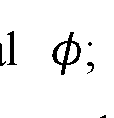 respectively, back-gate voltage dependence of momentum-resolved tunneling current in a MLG - MLG junction, Back-Gate voltage dependence of di /dV , and Back-Gate voltage dependence of d2I /dV2 ; Fig. 21 is a schematic of the MLG-MLG tunneling junction for experiments with a finite back gate voltage; Figs. 22a-b show measured and calculated d2I/dV2 vs. 9 and Vb, at VBG = —107 (similar to Figs. 20c, f); Fig. 23 shows determination of the electron lifetime at low bias; Figs. 24a-c shows a second toy model, explaining the momentum resolved features; Fig. 25 shows how the 'onset' and 'Dirac matching' features evolve between low temperature (kBT = ImeV,
RECTIFIED SHEET (RULE 91) ISA/EP
blue) and room temperature (kBT = 25meV, dashed red); Figs. 26a-g shows comparison of the second toy model with the measurements; Figs. 27a-e illustrate how the main features obtained in the experiments using toy models appear in the full calculation; Fig. 28 shows the energy band shift, (f>, as a function of Vb, (red dots) extracted from the feature that follows the MLG bands in the MLG-TBG measurement in Fig. 9d.
Fig. 29 (see the description in the section “Experiments with a probe of a smaller lateral size” below) shows an image of the whole area of sample detected by a probe fabricated by the inventors while being moved along the surface of the sample and imaged multiple times by the defects.
DETAILED DESCRIPTION OF THE ASPECTS AND EMBODIMENTS
Reference is made to Figs. 1A-C schematically exemplifying probes according to the three groups as mentioned above, respectively. Figs. 1A-C show side views of the probes.
A probe 10 of Fig. 1A is an exemplary probe which may be used for mechanically contacting a sample and conducting electrical measurements on the sample. It includes a tip presented in this example by a core 12 with an apex 12A. Also, probe 10 includes an active layer 16 presenting a 2D material of not more than 10 monolayers coupled by vdW forces, and a support layer 14 of a vdW material including layers 14-1 to 14-n. The active layer 16 is placed on the support layer 14 at the apex 12A; and it is further away at the apex 12A from the core 12 than the support layer 14. In other words, the active layer 16 and the support layer 14 form a vdW heterostructure covering the apex 12A, and the vdW heterostructure is turned with the support layer 14 towards the apex 12A. The active layer 16 at the apex 12A is exposed for contacting a sample.
In probe 10, a layer arrangement, covering apex 12A and including the support layer 14 and the active layer 16, i.e. their vdW heterostructure, has a plateau at the exposed layer. This plateau contains a square with a side of 10 nm or more. Hence, the contact area is expected to contain the square with a side of 10 nm or more under pressure against a planar surface.
The layer arrangement at the apex 12A in probe 10 conducts an electric current substantially, or even only, in a lateral dimension and substantially, or only, through the active layer 16.
RECTIFIED SHEET (RULE 91) ISA/EP
In Fig. 1A the active layer 16 extends away from the apex 12A, but along core 12 of the tip, and it stays exposed on the side of the tip, to which it is attached via the extension of the support layer 14. The extension of the active layer thus may be used for connecting to a contact electrode, which could lie on be pressed to the exposed extension of the active layer. In different examples, the active layer may extend away from apex 12A towards the contact electrode without being mechanically connected to the core 12. The contact electrode may be bulk and may be included into the probe, or it may be separate from the probe. For example, the contact electrode may be made on a side of the core 12 and be included into the tip as it’s another part, additional to core 12; or if the core 12 is grown on or attached to a substrate, the contact electrode may be made on a substrate. The active layer 16 may be on top of or beneath the contact electrode where they intersect.
In Fig. IB a probe 20 is shown. In this example, the probe includes an active layer 26 instead of 16; and it includes a tunnel barrier layer 28. Other elements are the same as in Fig. 1A. The active layer 26 may differ from the active layer 16 in some respects: on the one hand, active layer 26 does not have engage in a direct contact with the sample, but on the other hand it has to be compatible with tunnel barrier layer 28, for example, possibly to attach this layer to probe 20 if it is not attached to this probe in some other way (for example, to a substrate if it is included into the probe).
Fig. 1C shows an example of a probe 30 in which the active layer 26 is covered by a defect-assisted tunneling layer 38A, which is exposed. This defect-assisted tunneling layer 38A includes an at least one atomic defect 38B presenting a flow path for a tunneling current between the sample and the active layer 26. The layer arrangement, which at the apex 12A includes the defect-assisted tunneling layer 38A in addition to the hetero structure of the support layer 14 and the active layer 26, is allowed to conduct the electric current at least by tunneling through this defect-assisted tunneling layer 38A via the atomic defect 38B when the applied voltage coincides with the peak of the tunnel conductance of the defect, and then in a lateral dimension and through the active layer 26. By the “atomic defect” is meant either one or a complex (or cluster) of few missing atoms, one or a complex of few substitutional atoms, one or a complex of few interstitial atoms; or a complex combining defects from two or three of these types. Hence, the
current will depend on the free carrier density of state and the local electrostatic potential in the sample in a vicinity of the defect and the energy distribution of the carriers.
Fig. 2 schematically shows an example of a front view of a contact area CA of each of the probes 10, 20 and 30 against a planar surface. For probe 10, the exposed layer is the active layer 16; for probe 20, the exposed layer is the tunnel barrier layer 28; and for probe 30, the exposed layer is the defect-assisted tunneling layer 38A. In each case, the contact area contains a square SI with a side of 10 nm or more.
Fig. 3A provides an example how a contact electrode may be added to the probe, in accordance with one of the options mentioned above. In this example, probe 10A is similar to probe 10, but its active layer 16 extends along the core 12 further away from apex 12A than the support layer 14. The tip of the probe 10A is equipped with a contact electrode 18 grown, placed, or deposited on the core 12, and the active layer 16 extends to this contact electrode 18. Still, in all cases, according to another option the contact electrode may additionally or alternatively be deposited on top of the active layer.
Fig. 3B provides an alternative example with respect to how the active layer 16, the support layer 14 and the core 12 may be positioned with respect to each other on the side of the core 12. In this example, probe 10B is similar to probes 10 and 10A, but it has an active layer extension 16E of a shape with folds, and a support layer extension 14E of another shape with folds. This may happen, for example, due to a different combination of an angle of between the core side wall and the apex 12A and flexibilities of the active and support layers. In this example, the active layer extension 16E does not adhere to the support layer extension 14E at some segments of its length even though it covers the support layer extension as the most proximate layer from one side; i.e. in the present example there is a gap between the active layer 16 and the support layer 14 (even two such gaps in Fig. 3B). Similarly, support layer extension 14E does not adhere to the core 12 in its certain segment (however, it has to be remembered that the support layer extension and the active layer extension may adhere to each other in a differently oriented cross-section; and similarly for the support layer extension and the core).
Such gaps or spaces may be used to reduce a risk of tip crash: with a part of the layer arrangement bordering such a gap, this part (i.e. one or more of respective segments in Fig. 3B) may flex into it and/or out of it. Depending on the measurements (for example, cryogenic or not), such spaces may be filled with vacuum, or a fluidic matter, for example,
a gas, a liquid, or a gel, and thus allow the plateau of the desired dimensions at the apex to be formed upon the contact with the planar surface.
Fig. 4 schematically illustrates that a gate electrode layer 13 may be added to the probe. In this specific example probe 10C is based on probe 10, with the gate electrode layer lying between apex 12A and the support layer 14. However, a gate electrode layer such as the layer 13 also can be used in all other probes of the present disclosure. By applying a voltage bias between the gate electrode layer and the active layer, the properties of the active layer can be continuously modified, thereby allowing to change the properties measured in the experiment. Specifically, the changes may involve tuning the carrier density in the active layer, the density of states, and/or the workfunction of the active layer. Each of these parameters is useful for controlling the current measurement. For example, in the third embodiment (with the defect-assisted tunneling layer) a voltage bias between the gate electrode layer and the active layer influences the workfunction of the latter, which in turn gates the defect and shifts its energy level. The gate can thus be used to continuously tune the energy level of the defect.
Figs. 5A and 5B schematically illustrate that a probe may lack a plateau containing the square of 10 nm size on the exposed layer when it is not used, but in such a case its layer arrangement LA may have a convex surface region PP (a proto-plateau) flexing under pressure or mechanical contact with a sample into a plateau P containing such a square. This possibility is relevant to all probes according to the present disclosure (including the illustrated exemplary probes 10, 20, 30, 10A and 10B in those their modifications which without pressure lack the plateau covering the square of 10 nm).
Fig. 6 schematically shows an example of an SPM apparatus 100 according to the present disclosure. In the present example, the SPM apparatus is implemented as an AFM apparatus, but a skilled person would readily understand from Fig. 6 also how an STM apparatus may be configured according to the present disclosure: the AFM apparatus would be replaced with an STM apparatus, and an STM probe would be used instead of the AFM cantilever. This STM probe may be implemented as any of the probes in the present disclosure.
Hence, the AFM apparatus 100 includes a stage 102 to carry a sample, a head 104 to hold an AFM cantilever above the stage 102, an electric motor 106 for laterally rotating the stage 102 with respect to the head 104, and a control unit 108 for controlling the lateral
rotation of the stage 102 with respect to the head 104 with an accuracy better than 5 degrees, or 1 degree, or 0.1 degree, or 0.01 degree, or 0.001 degree to provide a desired orientation alignment between them. The arrow in Fig. 6 indicates the control. Fig. 6 represents both an AFM that works at room temperature and also an AFM that works at cryogenic temperatures.
Such a modification of the AFM according to the present disclosure is useful for conducting momentum-resolved measurements, to scan along the momentum space without disengaging the probe in the contact mode from the sample. Also, it is useful for forming a hybrid interface with a tunable twist angle and probing its physical properties at different twist angles. These properties as well may be local, for example, the local conductivity or carrier density.
The following section called “Additional Description”, and then related to it “Supplementary Information”, includes a description which, along with figures referred therein, provides some further details of the inventors' considerations and specific experiments, as well as more examples of probes corresponding to the disclosure above, including information on some fabrication techniques and results which such probes have already brought about:
Additional Description
The Quantum Twisting Microscope:
The scanning probe microscopy has revolutionized the way electronic phenomena are visualized. While present-day probes can access a variety of electronic properties at a single location in space, a scanning microscope that can directly probe the quantum mechanical existence of an electron at multiple locations would provide direct access to key quantum properties of electronic systems. Here, a conceptually new type of scanning probe microscope is demonstrated - the Quantum Twisting Microscope (QTM) - capable of performing local interference experiments at its tip. The QTM is based on a unique van-der-Waals tip, allowing the creation of pristine 2D junctions, which provide a multitude of coherently-interfering paths for an electron to tunnel into a sample. With the addition of a continuously scanned twist angle between the tip and sample, this microscope probes electrons in momentum space similar to the way a scanning tunneling microscope probes electrons in real space. Through a series of experiments, the inventors have demonstrated room temperature quantum coherence at the tip, studied the twist
angle evolution of twisted bilayer graphene, directly imaged the energy bands of monolayer and twisted bilayer graphene, and finally, applied large local pressures while visualizing the evolution of the flat energy band of the latter. The QTM opens the way for novel classes of measurements and experiments on quantum materials.
An electron in a solid is a quantum mechanical object best described by an extended wave function, reflecting its existence in a superposition of spatial locations. The STM dramatically changed how electrons in real space can be visualized. It was followed by a large array of other scanning probe techniques that now allow local measurements of various electronic properties. To date, existing scanning microscopes can only probe electronic properties apparently at one location at a time. Therefore they are unable to probe the interference of several tunneling trajectories, which would map the evolution of the quantum mechanical phase in space. To do so requires a scanning interferometer that probes an electron at several locations simultaneously and quantum coherently.
Thus, the inventors demonstrate a conceptually new type of scanning probe microscope - the Quantum Twisting Microscope (QTM) - capable of performing local interference experiments at its tip. The invented technique is based on a unique van-der- Waals (vdW) tip, which is brought into contact with a vdW sample, forming a 2D interface that can be twisted and spatially scanned with high angular and positional precision. The QTM enables at least two orthogonal and complementary classes of experiments: 1) “In-situ twistronics” - measuring a continuously twistable interface between a pair of vdW materials (e.g. twisted bilayer graphene). Here, the active vdW layers are placed in the tip and sample in direct contact, such that their wavefunctions strongly couple, and then the transport properties of the hybridized interface are probed. 2) Momentum-resolved tunneling - Here, a tunnel barrier (e.g. a few layers of a transition metal dichalcogenide) is inserted between the active vdW layers in the tip and sample. This barrier decouples their wavefunctions, allowing the tip to act as a momentum- resolved probe (non-invasive) for the sample’s energy bands. Since an electron can coherently tunnel into a sample at many locations along the 2D interface, this junction acts as an interferometer on a tip. Specifically, this implies that in the absence of electronphonon, electron-electron and impurity scattering, an electron would tunnel only between states of equal momenta. In this modality, the microscope’s twisting degree of freedom
is used for scanning an arc in the momentum space of the sample, and imaging along it the sample’s energy bands.
The QTM’s Operating Principle
To date, existing approaches for in-situ twisting experiments are based on electrical devices fabricated with a rotatable part and an external mechanical device, such as an atomic force microscope (AFM) tip, which pushes this part. The QTM of the inventors, in contrast, elevates the AFM tip to become an integral part of the twisted device, which is now split into two parts: the first is a standard vdW device formed on a flat substrate (Fig. 7a, Supp. Info. S2). The second is a vdW device formed on a specially- designed pyramid at the edge of an AFM cantilever (Fig. 7b, Supp. Info. S I). Both sides have independent electrical contacts. The inventors have used a commercial AFM to bring the two parts into contact and to maintain a constant force across the interface throughout the entire experiment (Fig. 7c). On the AFM stage, they have mounted a piezoelectric rotator with X and Y nanopositioners on top (Supp. Info. S3). This setup allows rotating the bottom sample with an angular resolution of 0.001° and positioning the point of interest in the sample at the center of rotation. In addition, the standard scanning capability of the AFM (in X and Y directions) enables lateral scanning of the tip across the sample.
A useful ingredient of the QTM is its tip design, facilitating the formation of a flat vdW at its apex. To achieve this in some non-limiting experiments, the inventors started with focused-ion-beam deposition of a platinum pyramid (~1.2 — 1.6/im tall) on a tipless AFM cantilever (Fig. 7e). This is followed by sequentially transferring graphite, hBN and the active vdW layer (e.g., monolayer graphene) on the pyramid using a polymer membrane. The graphite screens the substrate’s disorder potential, and the hBN acts as a spacer. Fig. 7f shows an AFM image of the resulting tip: visibly, the vdW stack forms a “tent” over the pyramid with three or more folds climbing up to the pyramid’s apex. At the apex, a flat plateau spontaneously forms in the vdW stack, whose corners are determined by the folds (Fig. 7g). The typical bending angles of the vdW tent (~10 — 30°) are smaller than the pyramid’s angle (~45°). Thus, apart from a small touching point at the apex, the tent is mostly suspended (Supp. Info. SI). Due to the flexural rigidity of the graphite/hBN layers, the formed vdW plateau is wider than the pyramid apex, resting on it as a pivoting point. Therefore, when this tip is brought into
RECTIFIED SHEET (RULE 91) ISA/EP
contact with the sample, the plateau self-aligns its tilt to become parallel to the sample. By varying the pyramid geometry and graphite/hBN flake thicknesses (typically tens of nanometers), the inventors have achieved plateaus of varying linear dimensions between 50nm and 1pm. These dimensions are small enough to make their QTM tip a local scanning probe, yet large enough (-1000 atoms across or more) for wavefunctions on the plateau to have a well-defined momentum (ΔP—1/1000 of the Brillouin zone size). Contrary to etched boundaries in lithographic devices, the active vdW layer on the plateau is continuously extended to the rest of the pyramid, avoiding dangling bonds or buckles. This setting makes the wavefunctions smoothly connect to the rest of the vdW layer on the pyramid. Fig. 7d overlays the measurement circuit on a schematic cross-section of the junction: a bias voltage, Vb, is applied between the two active layers (vdW crystals 1 and 2), and the corresponding current, /, is measured. Buried bottom and top graphite layers can serve additionally as bottom and top gates for the junction.
In-Situ Twistronics.
The inventors have started with a "twistronic" measurement of a twistable interface between two graphene monolayers (MLG) in direct contact. This interface has remained elusive for existing in-situ twistronics techniques since MLG easily crumbles upon twisting. Fig. 7h shows the MLG-MLG interface conductance, dl/dV, measured vs. twist angle, 0, at T = 300K. Throughout the entire measurement, the sample and tip are kept in continuous contact. The layers do not show any sign of locking at 9 = 0°, and the conductance traces are highly reproducible, highlighting the unique mechanical robustness of the QTM junction. The conductance is mirror symmetric around 0 = 30°, (0 -> 60° — 0), where its value is minimal. It rises continuously toward 0 = 0° but plateaus at small angles (|0| 4°) where it becomes limited by the resistance away from the tip (“contact resistance”). Similar to the measurements in graphite-graphite and graphite-MLG interfaces by other groups, the inventors have seen extremely sharp conductance peaks at 0 = 21.8° and 38.2°. At these angles, the two layers form commensurate stackings in real-space with a supercell (Fig. 7i).

On the origin of the large conductance enhancement at commensurate angles, the inventors contemplated the following. One possibility is a better real-space registry of the atoms in the two layers. However, by definition, whenever unit cells are commensurate
RECTIFIED SHEET (RULE 91) ISA/EP
in real-space, their corresponding Brillouin zones (BZ) are also commensurate in k-space, implying that at commensurate angles, momentum states are also matched. Specifically, at = 0° the Dirac cones of the two layers overlap at the comers of the 1st BZ, and at =21.8° they overlap at the corners of the 3rd BZ (Fig. 7i). The relevance of real vs. momentum space matching is directly connected to the quantum coherence of the 2D tunnel junction: in an incoherent junction, the tunneling events of electrons at different locations are independent, and sum up classically to yield the total current (Fig. 7j, top). In such a case only the real-space matching is relevant. Conversely, in a coherent junction, tunneling events at different locations interfere, yielding a tunneling current that is sensitive also to the local phases of the wavefunctions (Fig. 7j, bottom). Tn particular, tunneling is possible only between wavefunctions with matching energy and momentum.
Local Momentum Resolved Tunneling
To observe also the momentum conserving nature of the QTM the inventors have added a tunneling barrier between the two MLG layers (trilayer WSe2, Fig. 8a, top inset). This barrier suppresses the hybridization between tip and sample, enabling the tip to act as a probe for the unperturbed energy bands of the sample. The barrier also significantly increases the tunnel junction resistance, assuring that an applied bias falls predominantly across this junction and that the measurement is not affected by contact resistance even near 0 = 0°. Fig. 8a shows the measured tunneling current, I, vs. the interlayer bias, Vb, and 0 at T = 300K. Around 0 — 0°, I increases slowly with Vb at low bias, and then sharply increases along a curved-X feature in the 0 — Vb plane. Interestingly, this increase is followed by a sharp drop at slightly higher Vb. At much higher biases (~ 0.8R), I rises again, this time exponentially with Vb, and rather homogenously for all 0. Fig. 8b shows the measured conductance, dl/dV. Here, the sharp drop of I manifests as a strong negative differential resistance (NDR), as was seen previously in lithographic devices. Finer details are revealed when the inventors have plotted the second derivative, d2I /dV2 (Fig- 8c): in addition to the strong curved-X (dashed white lines), the inventors have observed a straight-X feature (dashed black lines), along which d2I/dV2 shows peaks (/dips) on the positive (/negative) bias side.
To understand the observed curved-X feature three points in the 0 — Vb plane (Fig. 8d) can be considered: at point 1 ( = 0°, small Vb,) the atoms of the two layers
RECTIFIED SHEET (RULE 91) ISA/EP
are registered in real-space and their energy surfaces are matched in momentum-space (Fig. 8g, panel 1). Increasing Vb while keeping 0 = 0° (point 2) maintains the real-space registry but offsets the relative energies of the Dirac cones. Consequently, for almost all energy slices within the bias window, the equal energy states have mismatched momenta (one such slice is shown in panel 2 of Fig. 8g). Thus, the observed drop of I is concomitant with the loss of energy -momentum-matched eigenstates in the two layers. By twisting the layers to a finite 6, while maintaining Vb (point 3), the layers lose the registry in real space but regain overlap of states in momentum space, enabling momentum-conserving tunnelling processes (Fig. 8g panel 3). Indeed, at this point the measured I becomes large again, demonstrating its momentum conserving nature. The inventors have estimated the level of momentum conservation from a plot of I vs. 0 at small Vb = 40mV (Fig. 8a, right inset). The extremely narrow peak (A0 & 0.2°) implies an excellent momentum resolution, -0.004 of the BZ size, comparable to state-of-the-art ARPES detectors. In the experiment in Figs. 8a-h, the back gate voltage is zero and the measurement shows a good symmetry between positive and negative bias directions, suggesting an overall charge-neutral system. Additional experiments with finite back gate voltages (Supp. Info. S6) further show a rich evolution of the features with the total charge in the system.
The inventors have compared their measurements to theory of momentum- resolved tunneling between twisted layers presented in Bistritzer, R. & MacDonald, A. H. Transport between twisted graphene layers. Physical Review B 81, 245412 (2010) See Figs. 8d-f. Since the quantum and geometrical capacitances of the junction are generally comparable, the applied bias divides into shifts of the chemical potential of the top and bottom layers, μT
 and an electrostatic potential shift between them, <p, namely, Vb = <P + PB ~ PT (fig. 8h). To calculate the tunneling current at any point in the 0 — Vb plane, the inventor have first determined μT, μB and <p by solving the above equation self-consistently with the equations-of-state of the individual layers, μT(nT) and μB(nb), (Supp. Info. S4). They then have summed the tunneling rates for all energy-momentum conserving tunneling processes within the bias window. We further add a Nordheim- Fowler contribution due to the breakdown of the WSe2 barrier. All expressions include the effects of finite temperature and lifetime. Overall, the agreement with the experiments has been excellent, both in terms of the locations of the various features, and
RECTIFIED SHEET (RULE 91) ISA/EP
in terms of their relative magnitude. The theory further has allowed the inventors to identify the experimentally observed features: the straight-X corresponds to the onset of momentum resolved tunneling, happening when the Fermi surface of one layer touches the empty bands of the other layer ('k-resolved onset' condition, Fig. 8f). The curved-X feature corresponds to nesting of the energy bands ('nesting' condition, Fig. 8f) Here, a macroscopically large number of energy-momentum conserving states become available to tunnel, explaining the large increase of / along this feature. With a further increase of Vb or a further decrease of 6 most of the states cease to be energy-momentum conserving, explaining the consequent large drop in I.
The simplicity of graphene’s dispersion has allowed the inventors to obtain analytic expressions for the k-resolved onset and nesting conditions. Specifically, for a non-interacting charge-neutral system, the onset condition becomes (Supp. Info S5) Vb = hvFKD9, where KD is the Dirac point momentum. Namely, Vb and 6 substitute the energy and momentum in the standard Dirac equation. Overlaying this expression on the measurement (dashed black lines, Fig. 8c) yields an excellent fit with vF — 1.05 ± 0.02 .1 106m/s, consistent with a measured Fermi velocity of graphene. Additionally, the nesting line provides the energy shift between the bands, </>, at any value of Vb, from which the electronic compressibility of the system can be straightforwardly determined (Supp. Info. S5). This measurement thus provides simultaneous information about the excitation spectrum of the system and its thermodynamic properties.
Momentum-resolved Imaging of Twisted Bilayer Graphene Energy Bands
Having probed the energy bands of MLG, the inventors have turned to a system with more intricate energy bands - twisted bilayer graphene (TBG). The experiment comprises of a MLG probe, a bilayer Wse2 barrier, and TBG with a 2.7° twist (Fig. 9a). In momentum space, the TBG mini-BZ hosts at its corners the Dirac cones of the underlying top and bottom graphene sheets (red and blue circles at Ktop and Kbot, (Fig. 9b). In the experiment, the MLG is rotated with respect to the TBG, and correspondingly its Dirac cone (purple circle, Fig. 9b) scans the energy bands of the TBG along a constant radius arc in momentum space (dashed purple arc, Fig. 9b), cutting precisely through Ktop and Kbottom and passing very close to the ΓM points of adjacent mini-BZ’ s. Along this k-space linecut, the TBG is theoretically predicted to
RECTIFIED SHEET (RULE 91) ISA/EP
exhibit the "flat bands" around zero energy and remote bands at higher energies (blue and black in Fig. 9c). Fig. 9d shows the dI2/dV2 measured vs. Vb and 6. The second derivative diminishes the smoothly evolving background, allowing to clearly resolve the key features. The measurement shows a wealth of features, the most prominent of which are traced in Fig. 9f. Interestingly, it exhibits a superposition of the ‘system’ and ‘probe’ energy bands, including the TBG’s flat bands (blue), remote bands (black), as well as two copies of the MLG Dirac bands (purple).
A theoretical calculation of the MLG-TBG momentum-resolved tunneling (Fig. 9e) shows excellent agreement with the experiment, down to small details. Specifically, the theory reproduces the features due to the flat and remote TBG bands, as well as the two displaced copies of the MLG Dirac bands. Furthermore, from the theory the inventors have been able to conclude that the band imaging is performed effectively by Dirac points: for example, when the MLG Dirac point matches in energy and momentum a state on the TBG flat bands (left inset, Fig. 9e), the d2I/dV2 exhibits a peak. This peak of d2I/dV2 corresponds to a minimum in /, reflecting the minimal tunnelling density of states at the Dirac point. Similarly, when one of the two TBG's Dirac points matches the MLG bands (right inset, Fig. 9e) a strong feature appears in dI2/dV2 (this time with an opposite sign, see toy model in Supp. Info S8). Consequently, the two TBG Dirac points trace out two copies of the MLG bands, displaced by Δθ = 2.7°. In addition to these Dirac matching' conditions that are insensitive to band filling, there are also 'onset' features, which appear whenever the Fermi level of one side (tip/sample) crosses the bands of the other side (for details see Supp. Info. S8).
The inventors have obtained the flat-band energy dispersion directly from the measurements by using the simultaneously measured MLG Dirac bands to calibrate the energy shift at each Vb (Supp. Info. S8). Fig. 9h compares the extracted e(k) of the flat bands (red and grey dots) with the prediction of the BM model (blue). The overall agreement is rather good, although the experiment shows an electron-hole asymmetry (-12% along the Kbot — M — Ktop branch and -20% along the Ktop —
 branch), contrasting the nearly-perfect e-h symmetry of in the BM model. The inventors’ measurements also reveal a quantity that is inaccessible to other probes - the layer polarization of individual wavefunctions at different momenta: visibly, when the MLG lattice is rotationally aligned with the top TBG layer (0 — +1.35°) the measured
RECTIFIED SHEET (RULE 91) ISA/EP
dI2/dV2 amplitudes are strong. In contrast, when the MLG is rotationally aligned with the bottom TBG layer (6 = —1.35°) they are substantially weaker. This highlights the fact that the experiment probes the weight of the wavefunction on the top layer. In Fig. 9i the inventors have plotted the magnitude of I along the traced flat band features (blue, Fig. 9f) between Ktop and Kbot (dots), and compared it with the layer polarization as a function of k from the BM model. The inventors have been able to see that this quantity is indeed a good proxy for the layer polarization.
Imaging Twisted Bilayer Graphene Energy Bands Under Pressure
The inventors have proceeded also to showing another unique capability of the QTM - its ability to apply a large local pressure while simultaneously imaging the way it affects the energy bands. Pressure provides a key tuning parameter for vdW materials, as it directly controls the interlayer tunneling. In TBG, this was predicted and shown to tune the flat bands in and out of the magic-angle condition. However, the challenges in cryogenic pressure cell transport experiments have limited such experiments to very few measurements. Here, instead, the inventors have used the ability of the AFM to apply /EV-scale forces across the small QTM junction to achieve GPa-scale pressures at the interface (Fig. 10a, inset).
Figs. lOa-c plots the measured di2 /dV2 vs. 6 and Vb, for the junction of Figs. 9a-i, but now under pressures of P = 0.01, 0.4, and 0.68 GPa. Each frame is taken with a constant pressure during twisting, and the results are reversible upon repeatable increase and decrease of pressure between frames. Visibly, with increasing P the flat bands gradually shrink toward zero Vb, whereas the remote bands get further away from zero Vb. To show this more quantitatively, in Fig. lOd the inventors have traced the flat and remote bands over a larger sequence of pressures. The inventors have been able to clearly see the opposite motion of the flat and remote bands with pressure (arrows). This contrasting response reflects a band anti-crossing that increases with P, as expected from increased interlayer tunneling. Converting Vb to the energy shift using the simultaneously measured MLG bands, the inventors have plotted the energetic width of the flat bands vs. P (Fig. lOe). Notably, the width shrinks linearly with P, reaching a 17% reduction at P = 0.68 GPa. This compares reasonably to the 6-14% reduction predicted theoretically. A naive linear extrapolation of the measurements conducted by
RECTIFIED SHEET (RULE 91) ISA/EP
the inventors would suggest that the bands of 2.7° TBG could become fully flat at P 4GPa, well within the pressures achievable by AFM without damaging graphene. This could lead to fully flat bands with a moire periodicity that is much shorter than in magic-angle TBG, and correspondingly to proportionally larger Coulomb interactions, potentially taking this system into uncharted regimes of strong interactions.
The QTM demonstrated here and based on the probes and techniques according to the present disclosure may be employed in industrial and scientific setting for characterization of various devices. Additionally, it may be used for creating highly controllable novel interfaces between a large variety of quantum materials. Specifically, it enables continuous control with 0.001° resolution of one of the critical parameters of these interfaces - their twist angle. In the Additional Description with Supplementary Information, the inventors have explored systems based on graphene and WSe2, but the technique should be applicable quite generally to a plethora of layered conductors, and superconductors.
In any case, in view of the above, it is clear that the inventors have enabled a novel scanning microscope that has direct access to the energy-momentum dispersion of electronic systems. As such, it may probe the dispersion of any excitation, charged or neutral, as long as it can be excited by a tunneling electron. The measurements can be performed at large magnetic fields, with variable carrier density and electrical displacement fields controlled by local gates, and with a continuously tunable pressure. As for the lateral scanning degrees of freedom of the QTM, they result naturally from its SPM (AFM or STM) platform. These degrees of freedom allow preforming spatially- scanned momentum resolved measurements within electronic devices with a high spatial resolution (~100nm). Lateral scanning also provides control over the lateral displacements between vdW materials, most likely down to atomic dimensions, capturing another key tuning parameter of the energy dispersions at these interfaces.
The following presents more details on Figs. 7a-j to lOa-e:
Figs. 7a-j: The Quantum Twisting Microscope setup and in-situ twistronics experiments, a, b and c, Illustrations of the components of the QTM. a. van-der-Waals (vdW) heterostructure assembled on a flat substrate with electrical contacts, b. vdW heterostructure assembled on a pyramid positioned near the edge of an atomic force microscope (AFM) cantilever, with electrical contacts. At the apex of the pyramid, the
RECTIFIED SHEET (RULE 91) ISA/EP
vdW-device-on-tip has a flat plateau, c. These devices are brought into contact using a commercial AFM, fitted with a piezoelectric rotator that allows to control the relative angle between tip and sample, 9, continuously with a 0.001° resolution, in addition to the usual lateral (X/Y) scanning capabilities of the AFM. d. Measurement circuit plotted over a schematic cross-section of the QTM junction. A voltage bias, Vb, is applied between the two active vdW layers (vdW crystals 1 and 2), and the corresponding current, /, is measured. Buried top and bottom graphite gate voltages, VBG and VTG, can modify the local carrier density and electric field in the junction (in this Additional Description with Supplementary Information, the top gate is physically shorted to the top graphene layer such that VTG is identically zero) e. SEM image of an AFM cantilever with a custom- made platinum pyramid deposited by a focused-ion-beam. f. The topography of a vdW- device-on-tip (graphite/hBN/monolayer graphene (MLG)), imaged by AFM. The vdW layers form a tent over the Pt pyramid, with folds (dashed white) leading to a flat plateau, g. Zoomed-in AFM image around the pyramid’s apex (peak-force-error signal), showing the spontaneously formed flat plateau, h. Measured conductance, dl/dV, vs. rotation angle, 9, between two graphene monolayers (MLG, top inset) in direct contact, Vb = 50mV, VBG = 0, T = 300/<. The two vdW devices are kept in continuous contact throughout the measurement, i, Real-space and momentum-space registry for the commensurate angles of 0° and 21.8°. j, Illustrations of the incoherent and coherent tunneling across the 2D junction: in the former, electrons tunneling at various locations are incoherent, and the tunneling is proportional only to the local wavefunction squared. In the latter, tunneling trajectories within the coherence length interfere, and the tunneling is sensitive also to the variation of the phases of the top and bottom wavefunctions along the junction.
Figs. 8a-h: Momentum resolved tunneling between two twisted graphene monolayers, a. Top inset: Schematic cross-section of the experiment, comprising of an MLG/trilayer WSez/MLG tunnel junction. The WSe2 tunnel barrier suppresses the hybridization between the MLG layers allowing one to probe the unperturbed energy bands of the other. Main panel: Tunneling current, /, measured as a function of rotation angle, 6, and interlayer bias, Vb, at T = 300/G Right inset: a plot of I vs. 9 at Vb = 40mV (along the black dashed line in the main panel). The peak's full-width-half-max (FWHM) is 0.2°. b. A lock-in measurement of the differential conductance, di /dV, as a function
RECTIFIED SHEET (RULE 91) ISA/EP
of 6 and Vb, showing strong negative differential resistance (NDR, blue) along a curved- X feature. The measurement shows a good symmetry between the positive and negative bias directions, c. The second derivative, d2I/dV2, vs. 0 and Vb, obtained by a numerical derivative of the data in panel b. The black and white dashed lines correspond to two specific alignment conditions between the bands, 'k-resolved onset' and 'nesting', shown in panel f and described in the main text and Supp. Info. S5 . d-f. Theoretically calculated momentum conserving tunneling /, dl /dV, and d2l /dV2 between two MLG layers spaced by a tunneling barrier, as a function of 0 and Vb, based on the Bistrizer-MacDonald expression for momentum conserving tunneling between rotated vdW layers. The calculation includes finite temperature, kBT = 25meV, and a finite inverse electron lifetime, where e is the electron energy and // is the chemical
 potential. y0 = 4mek, yx = 0.035 are the experimentally fitted values. The lifetime at low energies corresponds to a coherence length
 « 150nm, comparable to the size of some of the inventors’ tips, setting a lower bound on the decoherence by electronphonon and electron-electron interactions at room temperature. The illustrations show the relative alignment of the two Dirac cones at the 'k-resolved onset' and 'nesting' conditions, along the corresponding dashed black and dashed white lines, g. panels 1-3 illustrate the relative alignment of the two MLG layers in real space and momentum space, corresponding to points 1-3 in panel d. h. Schematic band alignment of the two layers under finite Vb and 0. Vb divides between shifts to the chemical potentials of bottom and top layers, μB and μT, and the energy band shift (=electrostatic potential shift), <p. The Dirac points are shifted in momentum by k = KD0, where KD is the momentum of the Dirac point.
Figs. 9a-i. QTM imaging of the energy bands of twisted bilayer graphene (TBG) a. Schematics of the experiment, comprised of an MLG/ bilayer WSe2/ 2.7° TBG tunnel junction b. The mini-Brillouin zone (BZ) of the TBG, with the Dirac cones of the underlying top and bottom layers (represented by blue and red circles) located at two K- points (Kbot and Ktop). Also shown are the ΓM points of adjacent mini-BZs. When the MLG probe layer is rotated with respect to the TBG, its Dirac cone (purple circle) traces the TBG energy bands along an arc in momentum space (dashed purple), crossing through the Kbot and Ktop points, and very close to the ΓM points, c. Theoretical energy bands of 2.7° TBG along the dashed purple arc in panel b, calculated using the Bistrizer-
RECTIFIED SHEET (RULE 91) ISA/EP
MacDonald model. The “flat” and remote bands are shown in blue and black, respectively, d. The second derivative, d2I/dV2, measured as a function of 0 and Vb at T = 300K-. e. Theoretically-calculated d2I/dV2 for this junction, as a function of 0 and Vb. The theory is based on the Bistrizer-Macdonald expression for momentum conserving tunneling and includes finite temperature, kBT = 25meV, and finite electron lifetime , = 0.02. The insets show the relative alignment
 of the MLG and TBG energy bands at two points in the 0-Vb plane. Left inset: the MLG Dirac point matches in energy and momentum a point on the flat TBG bands. Right inset: the TBG Dirac point matches in energy and momentum a point on the MLG Dirac band, f, Tracing of the main features of the measurement in panel d, including features related to the TBG flat (blue) and remote (black) bands, as well as two copies of the MLG Dirac bands (purple), h. The TBG energy vs. momentum dispersion (red and grey dots) determined from the measurement in panel d after converting Vb to the energy axis (see text), together with the bands of the BM model (blue), i. The magnitude of the tunneling current, /, traced along the features that corresponds to the flat bands (blue curves, panel f) between Kbot and Ktop (gray/red points for the positive/negative bias side). The inventors have normalized the current values by a constant to compare with the theory. Blue line: the theoretically calculated layer polarization of the wavefunction vs. momentum.
Figs. lOa-e. Imaging the effects of applied pressure on the TBG energy bands: a. inset: Illustration of the experiment - applying a fixed AFM force across the junction results in GPa-scale pressures at the interface. In the experiment the inventors have kept the pressure on while twisting, a-c. Measured d2I/dV2 vs. 0 and Vb for the junction in Figs. 9a-i, but under applied pressures of P=0.01, P=0.4 and P=0.68 GPa. T = 300K. d. Evolution of the TBG energy bands with P. In this figure the inventors have traced features that reflect the flat and remote bands as a function of pressure (see key). For every pressure, the inventors have plotted points that were obtained from tracing the relevant feature ('onset' feature for the flat bands, zero
 / contour for the remote bands). Visibly, with increasing P, the flat bands gradually shrink toward zero Vb while the remote bands shift to higher Vb (arrows), consistent with a pressure controlled anticrossing. e. The bandwidth at the M point of the TBG “flat” energy bands vs. P (red dots), determined from linecuts at 0 = 0°. The inventors have converted Vb to the energy from
RECTIFIED SHEET (RULE 91) ISA/EP
the simultaneously measured MLG Dirac bands (curved-X on the right side in panels a- c, see Supp. Info S8). Dashed line is a linear fit to the data. At the highest applied pressure (0.68 GPa), the bandwidth shrinks by -17%.
Supplementary Information (also called “Supp. Info” before):
51. Fabrication of vdW-device-on-tip
52. Fabrication of the flat devices
53. Configuring a commercial AFM for QTM experiments
54. Calculation of momentum resolved tunneling in a QTM junction.
S4.1. Solving the electrostatics of the QTM junction self-consistently
54.2 Momentum-resolved tunneling current calculation
54.3 Band structure of TBG based on Bistrizer-MacDonald model
54.4 Nordheim-Fowler Contribution and WSe2 barrier breakdown
55. Understanding MLG-MLG momentum resolved tunneling experiments
55.1 Momentum-resolved onset condition
55.2 Nesting condition
56. Additional experiments: back-gate dependence of MLG-MLG k-resolved tunneling
57. Electron lifetime in MLG-MLG k-resolved tunneling experiment
58. Understanding MLG-TBG momentum resolved tunneling experiments
58.1 First Toy Model - tracing energy bands with a Dirac cone.
58.2 Second toy model - explaining the k-resolved 'onset' features
58.3 Temperature dependence of 'onset' and 'Dirac matching' features
58.4 Comparing the second toy model with the experiment
58.5 The full calculation - origin of the features in the MLG-TBG k-resolved tunneling
SI. Fabrication of vdW-device-on-tip
To fabricate the vdW-device-on-tips, the inventors have started with commercial tipless AFM cantilevers with a nominal spring constant of K=40 [N/m], length L=232 [pm], width W=37[pm] and thickness T =7[pm]. The inventors have coated the bottom side of the cantilevers with 4/100 nm Cr/Au using an e-beam evaporator. This coating serves as the electrical connection for the active vdW layer and the buried graphite, such that they are at the same electrical potential. Next, the inventors have deposited
a ~ 1.2- 1.6 um tall platinum (Pt) pyramid with a ~ 2 um square base using focused ion beam (FIB) deposition (Figs. 1 la-c). The nominal size of the pyramids' apex is ~ 50nm.
To assemble the vdW-device-on-tip, the inventors have used the polymer membrane transfer techniquel. Briefly, the inventors have spin-coated polypropylene carbonate (PPC) onto a Si/(90nm) SiO2 wafer, followed by exfoliating graphene/hBN crystals. The inventors then have cut a window into a piece of adhesive tape and use it to pick up the PPC film with the target crystal. The crystal is then aligned and transferred on top of the platinum pyramid, followed by melting (~ 120 °C) and washing-off (acetone) of the PPC film to leave behind the vdW crystal. The inventors have assembled the vdW heterostructure by successive transferring and cleaning of each layer. For example, for the experiments done in this Additional Description and Supplementary Information where the active vdW layer on the tip is monolayer graphene, the inventors have started by transferring a graphite flake, ~ 20-40 nm thick, on top of the Pt pyramid, followed by an insulating hBN flake, ~ 20-40 nm. These two layers act as an atomically flat mechanical support for the active vdW layer (monolayer graphene), which is transferred at the last step. The thicker underlayers also define the shape of the plateau obtained at the tip apex. By varying the thickness of these layers, it is possible to obtain plateaus of variable sizes in the range of 50 nm to 1pm.
Figures lla-f: QTM tip characterization, a. SEM image of FIB deposited Pt pyramid on a tipless AFM cantilever b. Top view of Pt pyramid c. Cross-section of a Pt pyramid cut using local FIB cutting d. Optical image of an MLG/hBN/graphite vdW heterostructure on top of a pyramid e. AFM topography of vdW heterostructure in panel d. f. A linecut from the AFM topography of the vdW tent (red, taken along the dashed red line in panel e) overlayed with a schematic drawing of the Pt pyramid to scale. The top part of the pyramid is smaller than the plateau formed at the top part of the vdW tent.
S2. Fabrication of the flat devices
In this Additional Description with Supplementary Information, the inventors have performed two types of experiments: In-situ twistronics experiments, in which two MLG layers are brought into direct contact (without an insulating barrier in between) and the conductance of the combined system is measured as a function of the twist angle (Fig. 7h), and momentum resolved tunneling, in which the inventors have put a WSe2 barrier between the MLG probe and the system (MLG or TBG). Here, rotation is used to
RECTIFIED SHEET (RULE 91) ISA/EP
scan the momentum axis. For the former, the devices consist of MLG placed on top of an hBN substrate and a graphite gate (Fig. 12b). For the latter, the inventors have used MLG or TBG on top of hBN and graphite, but now have capped it from the top with 2-3 layer WSe2 (Figs. 12c, d). All inventors’ devices have been assembled using the standard dry transfer technique. Briefly, a polypropylene carbonate (PPC) coated poly dimethyl siloxane (PDMS) is used to pick up the hBN, MLG (or TBG created using laser cut and stack method), and WSe2 layers. The inventors have then flipped the stacks by depositing them onto a PMMA-coated PDMS, followed by placing them on the bottom graphite gate. The final heterostructure has been transferred on a ~100um wide and ~80um tall Si/SiCh pillar, with pre-pattered gold contacts reaching close to its edge (Fig. 12a). The reason for placing the stack on a pillar rather than on a flat Si/SiC>2 wafer is that this provides mechanical and geometrical flexibility for the tip rotation with respect to the sample, preventing them from touching each other at any point other than at the tip's apex. Next, the inventors have created the electrical contacts by transferring thin (~10nm) flakes of graphite to bridge the pre-patterned contacts and the MLG or TBG. Figs. 12b, c,d show the three variants of heterostructures used in the main text (MLG without tunnel barrier, MLG with tunnel barrier, TBG with tunnel barrier). After assembly, the heterostructures are cleaned by scanning them with an AFM in contact mode to remove polymer residues.
Figures 12a-d: QTM flat side substrate and devices, a. SEM image of a Si/SiC>2 pillar with pre-patterned gold contacts, b. Optical image of an MLG/hBN/graphite sample used for in-situ twistronics experiments (Fig. 7h). c. Optical image of a WSe2/MLG/hBN/graphite sample used for momentum resolved MLG-MLG tunneling experiments (Figs. 8a-h). d. Optical image of a WSe2/TBG/hBN sample used for momentum resolved MLG-TBG tunneling experiments (Figs. 9a-i and lOa-e).
S3. Configuring a commercial AFM for QTM experiments
The inventors’ QTM setup used in some experiments following the example of Figs. 13a-13c above has included two parts (1) A custom-built rotating stage housing the bottom devices (2) A commercial atomic force microscope (Broker Icon) for performing the AFM operations (Force feedback and lateral positioning). Hence, this section further exemplifies various options for configuration of the AFM (some of which are mentioned also in the claims below).
RECTIFIED SHEET (RULE 91) ISA/EP
The custom-built rotating stage comprises (from bottom to top): a goniometer, piezoelectric rotator (attocube), X and Y piezoelectric nanopositioners (attocube) and a sample holder with multiple electrical contacts (Fig. 13c). The goniometer compensates for the built-in angular tilt mismatch between the tip and sample sides in commercial AFMs (~12 degrees in our AFM) and reduces it to ~1 degree. The piezoelectric rotator has an optical encoder allowing for closed-loop angular control with ~1 milli-degree precision. The two linear nanopositioners, mounted on top of the piezoelectric rotator, position the device's point-of-interest in the center of rotation. This custom stage is attached using a rigid frame to an existing AFM stage (because of height limitations, the inventors had to connect it on a side facet of the AFM stage). This adapter has allowed the inventors to use the integrated optics and all standard AFM operations. The AFM has enabled inventors to bring the two vdW surfaces (in the tip and the sample) into contact. Additionally, inventors have used the active force feedback to maintain a constant force during rotation and measurement with a sub-nano-Newton precision. With this QTM setup, the inventors have employed two modalities for the rotation measurements.
(1) Continuous contact: Here, the inventors have brought the tip and sample together and rotated whilst maintaining the two surfaces in contact throughout the entire experiment.
(2) ’’Woodpecker'’: Here, for every point in the measurement as a function of rotation angle, the inventors have brought the tip into contact with the sample, performed the measurement, disengaged, then rotated by a small angle, and then repeated this sequence to get the full measurement. It should be noted that the inventors have obtained almost identical results from both modalities, and both have been highly reproducible.
Figures 13a-c: Room-temperature QTM measurement setup a. Custom-built rotator stage integrated into the side of a commercial AFM stage, b. Side view of the rotator stage facing the AFM scanner and optics, c. The components of the custom-built rotating stage.
S4. Calculation of momentum resolved tunneling in a QTM junction.
In this section the model is presented used by inventors for calculating the theory panels in Figs. 8a-h and 9a-i. In addition to the parameters that are scanned in the experiment that are shown in the main text - the twist angle, 0, and bias, Vb, the inventors also have included in the model the effect of back gate voltage, VBG, such that it also describes the experiments at finite gate voltages shown in section S6 below. The tunneling
RECTIFIED SHEET (RULE 91) ISA/EP
current is calculated separately for each combination of the parameters 0, Vb, VBG. The inventors first have determined the chemical potential of top and bottom layers and the electrostatic potential shift between them by solving the electrostatic
 equations (S4.1, S4.2) self-consistently with the equations-of-state of the individual layers: and This is described in section S4.1 below. The inventors then

 have summed up the momentum-conserving tunneling rates for all states within the energy window opened by the bias, between μT and μB. This is described in subsection S4.2 below. The equation of state for the TBG is obtained from the Bistrizer-Macdonald continuum model, detailed in section S4.3. Finally, the inventors have added aNorhdeim- Fowler term due to the breakdown of the WSe2 barrier, described in section S4.4. All expressions include the effects of finite temperature and finite lifetime.
S4.1. Solving the electrostatics of the QTM junction self-consistently
The inventors have described the electrostatics of the QTM tunnel junction by a three-plate-capacitor model. The first two plates are the top and bottom active vdW layers (in the tip and sample), which are separated by a tunnel barrier (2 or 3 layers of WSe?). The third layer is the graphite back-gate, separated by an hBN spacer from the bottom vdW system. The inventors have derived the two following equations:
 where Vb is the applied bias between the top and bottom layer, VBG is the back gate voltage with respect to the bottom layer, and μB, nB, μT and nT are the chemical potential and carrier densities of the bottom and top layer respectively. The geometric capacitance per unit area between top and bottom layers, Cg, and between the back-gate and bottom layer,
CBG, are given by: 3) 4)
 where dws 2is the barrier thickness (taken to be 0.58nm per monolayer of WSe2), dBN is the hBN thickness (70nm in the MLG-MLG experiment) in Figs. 8a-h, and 3.2 are taken to be the corresponding dielectric constants. For

RECTIFIED SHEET (RULE 91) ISA/EP
MLG, the dependence of carrier density on chemical potential is given by the Fermi velocity. For TBG, is

 calculated numerically from the Bistritzer-MacDonald continuum model (section S4 below). We solve together the above equations for gB,gT and </>, self-consistently. Due to the low carrier density of graphene, the quantum capacitance of the QTM junction is generally of a similar order of magnitude as its geometric capacitance. Consequently, the applied bias changes the chemical potentials of the layers as well as the electrostatic potential between them . In Fig. 14 the inventors have plotted the dependence of vs. Vb calculated for the parameters of the MLG-MLG
 experiment in Figs. 8a-8h in the main text. The inventors have been able to see that in this experiment, a change of Vb indeed leads to a same order of magnitude of change in all these quantities. It can also be seen that due to the assumption of overall
 charge neutrality, which describes well the experiment in Figs. 8a-8h with VBG = 0. As explained in section S5, experimentally, it is possible to directly determine the dependence from the nesting line in Fig. 8c. Specifically, the inventors have seen
 that the nesting feature in Figs. 8c, f fits well the experiment if we take Cg = 2.35gF/cm2, consistent with thickness and dielectric constant values mentioned above.
Figure 14. The bias dependence of top/bot
 tom chemical potential and
 electrostatic potential for MLG-MLG tunneling junction.

S4.2 Momentum-resolved tunneling current calculation
After solving the electrostatics and obtaining the chemical potential and band alignment between top and bottom layers, the inventors have proceeded to calculate the tunneling current. The theoretical model is based on the Bistritzer-MacDonald expression for momentum resolved tunneling between two layers. The model assumes that the tunneling is well described by Fermi's golden rule, namely, that a carrier tunnels coherently only once across the junction and not multiple times back and forth. This assumption is valid for all the experiments in the Additional Description with Supplementary Information that involve a tunneling barrier between the two vdW layers and is implied from the fact that the resistance of the tunnel junction is much larger that the resistance along the vdW layers themselves. With these approximations, the tunneling current is given by:
RECTIFIED SHEET (RULE 91) ISA/EP

Here gs = 2 accounts for the spin degeneracy. The functions fB(E) and fT(E + 0) are the Fermi-Dirac distribution functions of the bottom and top layers, while <p is the electrostatic potential that shifts the relative position of energy bands. is
 the tunneling matrix element between a state with momentum kT on the top layer to one with momentum kB in the rotated Brillouin zone of bottom layer. The functions AB and AT are the spectral functions for the bottom and top layers: A
 where eT (fc) is the energy bands of the top layer. yT is the corresponding inverse electron lifetime (the inventors elaborate on this lifetime in section S7). Similar formula applies to the bottom layer.
Eq. (S4.5) requires three conditions to be met for a tunneling event to be allowed. The Pauli principle require the tunneling electron to originate from a full state and arrive to an empty state. This is imposed by the difference between the two Fermi functions. Energy conservation requires the energy difference between the state of origin and the state of destination to differ by <p. This is encoded in the energy arguments of the Fermi functions and the spectral functions. And momentum conservation requires the states of origin and destination to have the same momentum. These three requirements are typically met by a curve in momentum space, whose characteristics are determined by p.b,gt, <p and, most importantly, by the energy spectra of the two layers. The contribution of the states along that curve is determined by the density of states and by the value of the tunneling matrix element at that momentum.
Following Bistritzer-MacDonald, the tunneling matrix element is given by:
 where \ukr and are the wavefunctions on the top and bottom layers, s
 and s' are the band indices, primed wave vectors are rotated with the twist angle, GT, GB are reciprocal lattice vectors of the top and bottom layers, α, β are sublattice indices, and 's l'lc Fourier transform of the finite -range interlayer hopping amplitude
 (discussed below). In a matrix form in the sublattice basis the tunneling matrix element is given by:

Here and are the sublattice positions of atoms A and B within the unit cell

 of the top layer; dT is the lateral displacement vectors for these two layers. The BM model assumes that the tunneling amplitude tk' +Gb decays exponentially with the absolute value of momentum measured with respect to the origin in momentum space. Thus, the inventors have considered tunneling events within the first Brillouin zone and approximate which is independent of momentum. Consequently, in the
 summation of GT and GB reciprocal lattice vectors to obtain TG G only three processes are relevant:

In addition, the tunneling amplitude t0 is affected by the energy of tunneling electrons and the tunneling barrier shape (z). This is described by the WKB

Ac is the distance from the Dirac point to the conductance band edge of WSe2 relative to the graphene. E is the energy of the tunneling electron, d is the barrier width and m* is the effective mass in the z direction of WSe2, where the inventors have assumed a parabolic dispersion. The inventors have considered here only the conduction and not the valence band edge since it is significantly closer in energy to the Dirac point. The inventors have also ignored the in-plane momentum dependence of Ac.
S4.3 Band structure of TBG based on Bistrizer-MacDonald model
The inventors have used the continuum model to calculate the band structure of
 a0 = 0.142nm is the carbon-carbon bond length and the sublattice
 vectors A, B are SA = ao(O,O), δB = ao(O,l). The Hamiltonian is given by
 sublattice index s and valley index R± is the rotation matrix of top and bottom layer by twist angle The interlayer coupling matrix is given by:
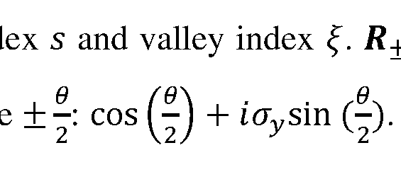
 the interlayer distance. wAA is smaller than wAB due to the lattice reconstruction in the
AA region, and we adopt the value: wAA = 88meV, wAB = 110meV.
S4.4 Nordheim-Fowler Contribution and WSe2 barrier breakdown
In the MLG-MLG junction, the tunneling spectrum shows a breakdown of the WSe2 tunneling barrier. This is modeled within the WKB approximation. At large bias, the bending of the WSe2 bands is large enough such that electrons can directly tunnel from the graphene into the conduction band states of WSe2. This is the Nordheim-Fowler field emission regime, described by:


Assuming that Ac is momentum independent, then the tunneling current is also momentum independent, and is given by:

The inventors have found the values m* = 1.07me and Ac = 0.55eF fit the experiments, consistent with the values reported in the literature.
S5. Understanding MLG-MLG momentum resolved tunneling experiments
In the MLG-MLG momentum-resolved tunneling experiment the inventors have identified two main features in the measured d2I/dV2 vs. Vb, and 0 (Fig. 8c): lines of momentum resolved 'onset' condition, appearing along a straight-X feature, and 'nesting' lines, appearing along a curved-X feature. In this section, the inventors have derived the equations that describe these conditions for the case of a charge-neutral system. The experiments in the Additional Description, performed with VBG = OF, are to a very good approximation a charge-neutral system. By comparing these experiments to the formulas derived here, the inventors have extracted the density dependence of the Fermi velocity and electronic compressibility in this system. In the next section the inventors will show additional measurements done with non-zero VBG, and derive the corresponding equations for the general case of a non-charge-neutral system.
In the charge-neutral case, the carrier density of the bottom layer is equal in magnitude and opposite in sign to that in the top layer: nT = — nB (S5.1)
Since MLG is electron-hole symmetric to a good approximation in the energy range probed in our experiments, Eq. S5.1 translates to:
E-T = ~EB = E (S5.2)
The electrostatic equation that connects the applied bias, chemical potentials in the two layers, and their relative energy band shift (=electrostatic potential, reads
 (illustrated in top panel, Fig. 15): (S5.3)

Figure 15. Schematic of the charge-neutral MLG-MLG tunneling experiment (Figs. 8a- 8h in main text). The main panel shows the analytically derived lines in the 0 — Vb
RECTIFIED SHEET (RULE 91) ISA/EP
plane, which correspond to the momentum-resolved 'onset' and 'nesting' conditions. Right and left insets show the theoretically calculated energy band alignments at select points along these lines. Top inset shows how the bias divides between the chemical potential of the two layers, nd the relative electrostatic energy shift of
 the bands, <p.
S5.1 Momentum-resolved onset condition
At a given bias voltage, momentum conserving tunneling onsets when the Fermi surface of one layer touches the empty bands of the other layer. For the charge-neutral case, this condition happens simultaneously for the Fermi surfaces of the top and bottom layers (right and left insets, Fig. 15), when:
 (S5.4)
Combining equations S5.4 and S5.3, the inventors have got a simple relation for the onset condition, (S5.5)

Effectively, this relation is the Dirac equation of graphene, but with energy E and momentum k replaced by Vb and KD0, respectively.
This simple relation appears only in the charge neutral case (the general case is discussed below), which is a good approximation for the experiments performed at allowing the inventors to directly compare them with equation S5.5. In Fig.
 16a the inventors have plotted the measured d2I /dV2 in the MLG-MLG (reproduced from Fig. 8c) and trace the peaks (dips) that occur at positive (negative) bias at the onset conditions. The points obtained from this tracing, shown by black dots in Fig. 16b, fit well a linear Dirac dispersion (blue) with a Fermi velocity ofvF = (1.05 ± 0.02) * 106m/s, consistent with previous measurements in graphene. In principle, the Fermi velocity in graphene is known to be renormalized by interactions and becomes logarithmically faster as the energy of the electrons approaches the Dirac point. This renormalization depends on the fine structure constant in graphene a — e21 ehvF. Since a depends on the dielectric coefficient of the surrounding environment, when graphene is encapsulated in a dielectric material (in our case WSe2 and hBN at its opposite sides), the value of the fine structure constant is close to one, and the velocity renormalization is rather small, about 10% change in velocity per one decade in energy. The inventors’ experiments have had two MLG layers, which screen better than the single MLG. On length scales larger than the separation of the two MLG layers (~ Inm in our experiment),
RECTIFIED SHEET (RULE 91) ISA/EP
they act as a single layer with double the density of states, effectively dividing the relevant fine structure constant, and the velocity renormalization by another factor of 2. The red curve in Fig. 16b shows the renormalized velocity calculated for our case. Visibly, the effect of renormalization is small, and within the errors in the determination of the onset peaks, both renormalized and un-renormalized expressions for the Fermi velocity fit well. d21
Figures 16a-b. a. Measured from Fig. 8c, where the inventors traced the local
 maximum (minimum) at positive (negative) bias, along the ‘onset’ features (black dots), b. Plot of the black dots from panel a together with bare Dirac dispersion (Eq. S5.5) with vF = 1.05 . 106m/s (blue) and Dirac dispersion that is renormalized by interactions.
S5.2 Nesting condition
Nesting between the Dirac bands of the top and bottom layers happens when these bands overlap along a line of the Dirac dispersion. In this situation, a large number of energy-momentum conserving states become available to tunnel between the layers. Unlike the onset condition, the nesting condition is independent of the band filling, and therefore it directly probes the energy dispersion. At a given twist angle 9, the Dirac dispersion of one of the MLG is shifted in momentum by k = KD9 relative to the other. Shifting the Dirac bands in energy by
 (S5.6) will bring the two MLG Dirac dispersions into nesting. This condition is similar to the onset condition in equation S5.5, except that here replaces Vb.
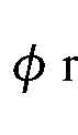
The nesting line in the measurement allows us to read out directly the energy shift between the bands for every Vb. Figure 17a plots the measurement after rescaling the rotation angle axis using equation S5.6. In these new axes the nesting line gives directly W)-
Once the dependence <p(Vb') is determined from the measurement, it is straightforward to obtain from it the geometric capacitance, Cg, and quantum capacitance,
Cq, of the system. By differentiating Eq. S5.3 with respect to , the inventors have
 obtained,
 which provides a direct relation between the local slope of the nesting line and the ratio of geometric to quantum capacitances. Hence, for system with different geometric
RECTIFIED SHEET (RULE 91) ISA/EP
capacitances the nesting line will have a different shape. This is demonstrated in Fig. 17b, which shows the theoretically calculated graphs with increasing value of Cg between the different panels. For the case of a smaller geometric capacitance (left panel, Fig. 17b), the slope of the nesting line approaches 1, as required by Eq. S5.7. In this limit, which corresponds to the case of a thick tunneling barrier, most of the applied bias goes into shifting the bands, and only a small fraction of it goes to increasing the chemical potentials. In the opposite limit (right panel), where the geometric capacitance is large (corresponding to a thin barrier), the bias hardly shifts the energy bands but mostly changes their occupation. The center panel in Fig. 17b has a nesting line that matches closely the dependence observed in the experiment (Fig. 17a). This has allowed the inventors to determine the geometric capacitance in this experiment to be
 The inventors could see that for a typical width of tunneling barriers (2-4 monolayers) and with the typical density of states of MLG, the experiments are generally in an intermediate regime in which the geometric and quantum capacitances are of comparable magnitude. Eq. S5.7 also shows that once Cg is determined, the local slope of the nesting line provides the quantum capacitance of the system. Eq. S5.7 was derived for the symmetric (charge-neutral) case of two MLG layers. In the general case when two systems are different, or they are the same but have different carrier densities, then 2 /Cq in Eq. S5.7 should be replaced by the in-series sum of the quantum capacitances of the two systems,

Figures 17a-b. Rescaling rotation angle 9 to the electrostatic potential <p. a. d2I measurement from Fig. 8c with 0 axis converted to <p using the relation
After rescaling, the nesting line (yellow extracted from peak fitting) gives directly b Calculated spectrum for geometric capacitances


S6. Additional experiments: back-gate dependence of MLG-MLG k-resolved tunneling
In Figs. 8a-h the inventors have showed momentum resolved tunneling experiments between two MLG layers. Here the inventors have presented additional data, showing how these measurements evolve with back gate voltage. Figures 18a-f-20a-f show measurements of /, dl/dV and d2I/dV2, respectively, vs. 9 and Vb, now as a function
RECTIFIED SHEET (RULE 91) ISA/EP
of back gate voltage. The top row in each figure shows measurements done at three values of the back-gate voltage, VBG = —10k, Ok, +107. The bottom row shows the corresponding theoretical calculations, based on the BM expression for momentum resolved tunneling between two parallel layers. Whereas the measurement at VBG = Ok is symmetric between positive and negative bias, the measurements at VBG = —10k, +10k are asymmetric in bias. Focusing on the measurements of d2I /dV2 (Figs. 20a-f), in which the features are the sharpest, we can see that while for VBG = 0k the crossing point of the curved-X is at zero bias, for finite VBG it shifts to finite bias (positive bias for VBG = + nd negative bias for VBG = —10k). Tn addition, the symmetric X shape at VB
 G evolves into a “bell-shape” that is asymmetric with respect to bias. However, if the inventors flip the bias axis and the sign of the current in the VBG = —10k measurement it becomes almost identical to the measurement at VBG = + 10k. Namely, the data obeys the following symmetry:


To interpret the experiments with finite back-gate voltages, the inventors have allowed for the chemical potentials of the two layers to be different and have generalized the analysis to include a finite VBG, following equations S4.1-S4.4. The resulting 'onset' and 'nesting' lines in this more general case are shown in Fig. 21. The inventors have seen that the theory recovers the asymmetric bell-shaped 'nesting' line, observed experimentally. This shape generalizes the functional dependence of < vs. Vb (Eq. S5.7)
 to now include two unequal inverse quantum capacitances in the layers, which add in series. In addition, the inventors have seen that now each 'onset' line splits in two, since the Fermi surfaces in both layers have a different size and they touch the empty bands in the other layer at different twist angles.
Figs. 22a-b overlays the calculated 'onset' lines on the measured d2I/dV2 at VBG — —10k, as well as on the corresponding theoretical calculation. Although room temperature smearing has almost eliminated all the detailed structure related to the 'onset' conditions, the inventors still have been able to resolve in the experiment faint peaks that follow the predicted 'onset' lines. Another feature that is clearly visible both in theory and experiment are the horizontal lines (dashed black) along which the d2I /dV2 flips sign. Each such line corresponds to one of the MLG layers going across charge neutrality,
RECTIFIED SHEET (RULE 91) ISA/EP
namely either
 = 0. Overall, the inventors have been able to see that the theory captures most of the details in the experiment rather accurately.
Figures 18a-f: Back-gate voltage dependence of momentum-resolved tunneling current in a MLG - MLG junction a-c. Tunneling current, I, measured in the junction in Figs. 8a-8h (MLG/ trilayer WSeo/MLG) as a function of 0 and Vb, for three values of the back-gate voltage VBG = +107, OF, — 107 respectively, d-f. Corresponding theoretical calculations
Figures 19a-f: Back-Gate voltage dependence of dl/dV. The same measurement as in Figs. 18a-f but now showing the (simultaneously measured) conductance, dl/dV. a-c. Experiment, d-f. Theory.
Figures 20a-f: Back-Gate voltage dependence of d2l/dV2. The same measurement as in Figs. 18a-f,19a-f but now showing the second derivative, d2I/dV2, obtained by numerically deriving the data in Fig. 19. a-c. Experiment, d-f. Theory.
Figure 21: Schematic of the MLG-MLG tunneling junction for experiments with a finite back gate voltage. The main panel shows the theoretically derived lines in the 0 — Vb plane, which correspond to the momentum-resolved 'onset' and 'nesting' conditions. Compared to the charge-neutral case, the 'nesting' line becomes "bell-shaped" and asymmetric in bias, and the 'onset' lines splits to four lines. Right and left insets show the theoretically calculated energy band alignments at select points along these lines. Top inset shows how the bias divides between the chemical potential of the two layers, jiT and [ B, and the relative electrostatic energy shift of the bands, < >.
Figures 22a-b. a. Measured and b. Calculated d2I/dV2 vs. 0 and Vb, at VBG = — 107 (similar to Figs. 20c, f). The overlaid black dotted lines correspond to the theoretically calculated k-resolved 'onset' conditions, as shown in Fig. 21. Horizontal dashed lines indicate the two biases at which each one of the MLG crosses through charge neutrality ( /B = 0 or μT = 0).
S7. Electron lifetime in MLG-MLG k-resolved tunneling experiment
The dominant mechanism setting the width of the features in the inventors’ measurement is thermal smearing. All measurements so far have been performed at room temperature, leading to kBT ~25meV smearing entering via the Fermi-Dirac functions in Eq. S4.5. To quantitatively explain our data, we find that we should also include smaller smearing due to finite electron lifetime. The electron lifetime is encoded in the spectral
RECTIFIED SHEET (RULE 91) ISA/EP
functions of the bottom and top layers, and
1 J

AT(e, k) = where eB(fc) and €T(k~) are the energy bands of these layers,
 and YB’YT are their corresponding inverse electron lifetimes. Finite lifetime leads to a Lorentzian broadening of the spectral functions, which could be directly observed in the width of the features in the measurements.
Fig. 23 plots the measured I vs. 0 at small bias, Vb — 40mV, (black line, same as the inset in Fig. 8a in the Additional Description). Compared with theoretical curves broadened by kBT = 25meV and with various inverse lifetime values, y0, we see that the value that best fits the measurement is y0 ~ 4meV. At higher biases (of the order of the Fermi energy) the inventors generally have observed shorter lifetimes. The dependence of the lifetime on energy is expected to be complicated in this energy range. The inventors have found a reasonably good fit to the phenomenological expression used previously,
 0.035.
The data shown in Fig. 23 allows for determining the electron lifetime at low bias. Black curve corresponds to the measured tunneling current, I vs. rotation angle 0, at small bias Vb — 40mV, for the junction in Figs. 8a-8h (same as he right inset in Fig. 8a). Colored curves in the figure correspond to the theoretically calculated k-resolved tunneling current (see text) with room temperature broadening kBT = 2SmeV and various values of inverse electron lifetime, y0 (see key).
S8. Understanding MLG-TBG momentum resolved tunneling experiments
In this section, the inventors explain the various features observed in the momentum resolved tunneling experiments between MLG and TBG, shown in Figs. 9a- 9b. The inventors first have used a simple toy model to explain the main mechanism leading to the quantitative energy band mapping in their experiment - tracing the bands of the sample with a Dirac point of the probe. As the inventors show, this mechanism directly probes the dispersion of the bands and is insensitive to their filling. The inventors then expand the discussion to include additional momentum-resolved tunneling 'onset' features that appear when the Fermi level of one side (tip/sample) crosses the energy bands of the other side. The inventors end by showing how these features appear in the full momentum resolved calculation, which includes the multitude of energy bands obtained within the BM model of TBG as well as finite temperature effects.
RECTIFIED SHEET (RULE 91) ISA/EP
S8.1 First Toy Model - tracing energy bands with a Dirac cone.
Here the inventors show the ability of using a Dirac cone to trace the energy bands of a sample, i.e., a method to read off the samples band structure. The inventors conceive a toy model of a probe layer with a Dirac dispersion scanning a system with arbitrary energy bands. For simplicity, we set the tunneling matrix element to be a momentumindependent constant. The results of the toy model depend on the relative Fermi velocity of the probe and system: vFprobe and vFsyst . Close to the intersection point with the probe’ s dispersion, the system’s band can be linearized with Fermi velocity vFsyst. The energy offset between the Dirac point of the probe and the system’s band is denoted by Ac. This offset can be tuned by changing the bias voltage between the probe and the system. The inventors have considered three situations: 1.
 3. vFprobe < vFsyst. The tunneling occurs in an energy window set by the bias voltage, where the states in the system are empty and the states in the probe are full (or vice versa). The inventors denote this energy window by £ < £ < E2. For simplicity, the inventors set T = 0 and neglect the electron lifetimes (i.e., the inventors treat the electrons as free).
In the case where vFprobe > vFsyst, the intersection between the energy surfaces of the probe and the system is an ellipse. The inventors assume that the entire ellipse is contained within the energy window [E17 E2] where the tunneling takes place. Then, using Eq. (S4.5), we obtain:
 where TTB is the tunneling matrix element. Hence, the current is minimal when the Dirac point coincides the system’s dispersion (|AE| -> 0). At this point, d2l/dV2 is strongly peaked. Thus, in this situation, the peak in d2l/dV2 can be used to directly read off the system’s band structure (see Figs. 24a, b). In the limit the size of
 the elliptical intersection between the two dispersion diverges, and it extends outside the window Hence, Eq. (S10.1) is not applicable in this limit.
If the intersection between the energy surfaces is a p 1 arabola. The
 tunneling current is
RECTIFIED SHEET (RULE 91) ISA/EP

Interestingly, the current diverges as |Ae| -* 0. This divergence corresponds to the nesting condition in the MLG-MLG tunneling junction. The divergence is regularized by introducing a curvature to the bands, or a finite lifetime of the electrons in the system and the probe.
Finally, for the intersection is a hyperbola. In this case, the
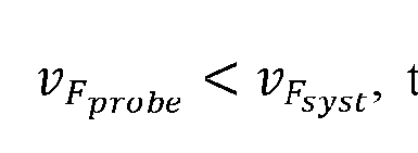 singular part of the current at small |Ae| is

I.e., in this case, the current has a maximum at Ae = 0. At this point, d2I/dV2 shows a minimum. This is the case for the Dirac point of TBG - with slower Fermi velocity - tracing the MLG dispersion.
S8.2 Second toy model - explaining the k-resolved 'onset1 features
In the previous section the inventors have explained the main features in their experiment that visualize the energy bands as resulting from tracing with a Dirac point. Tn addition to these, the inventors have seen features in the measurement (Figs. 9a-i) that correspond to 'onset' conditions of the momentum resolved tunneling. These occur whenever the Fermi surface of one side (tip/ sample) crosses the energy bands of the other side. In this section, the inventors use a more elaborate model that captures these 'onset' features and identifies their origin. The inventors will further show that these 'onset' features are strongly smeared by temperature, whereas the 'Dirac matching' features discussed in the previous subsection are largely insensitive to temperature.
To capture the essential physics, the inventors have used a second toy model that includes Dirac bands that represent the MLG and two parabolic bands, which mimic the conduction and valence flat TBG bands along
 the Kbot — M — Ktop trajectory in momentum space. In addition, the model also keeps track of the chemical potentials in both systems. The Dirac and Parabolic bands are shown explicitly in Fig. 24a. For simplicity, the inventors have focused only on a relative rotation angle of 0 = 0° between the MLG and TBG and calculate the current and its derivatives as a function of bias. Figure 24b, shows / vs. Vb calculated within this model, assuming a low temperature (kBT = ImeV). The corresponding d2I/dV2 is
RECTIFIED SHEET (RULE 91) ISA/EP
shown in Fig. 24c. For the electrostatics, the inventors have assumed a simple linear relation between the chemical potential of the layers and the applied bias, .T — — 0.41^ = 0.2Vj), which approximates rather well the full electrostatics of the real MLG- TBG junction.
At small Vb, the current is zero since there are no energy -momentum conserving states in the tunneling energy window (represented by a white window in Fig.24a and insets to Fig. 24b) between the chemical potentials of the two layers (red and blue dashed lines). Then, at a finite Vb (~0.18V for the parameters of Fig. 24b), the current exhibits a sharp step increase, that occurs when the Fermi level of the Dirac band (red dashed) crosses the occupied parabolic energy bands (left inset, Fig. 24b, crossing indicated by the black arrows). This is the 'onset' point where momentum conserving current first becomes available. At this bias, at zero temperature, the current discontinuously jumps to a finite value because a full circle of energy-momentum conserving states shared by the Dirac and parabolic bands becomes abruptly available. In the second derivative, d2I /dV the step of I shows up as a plus-minus dipole (Fig. 24c). With a further increase of Vb, the Dirac cone shifts down with respect to the parabolic bands and the circle of energy-momentum matched states (now deep below the Fermi energy) shrinks. Consequently, the current decreases linearly with Vb. It reaches a minimum when the Dirac point exactly crosses the parabolic band and the circle shrinks to a single point (center inset, Fig. 24b). In the second derivative, this minimum translates to a peak. This is the ‘Dirac matching’ condition, discussed in the previous section. Upon a further increase of Vb, the energy-momentum conserving circle of states grows back again, leading to a linear increase of /, until a second onset condition occurs, where the Fermi level in the parabolic bands (dashed blue) crosses the empty Dirac bands (right inset, Fig. 24b). This second onset leads to another step in 1 and to a second diploe in d2I /dV2.
The calculation in Figs. 24a-c was performed with a low temperature, such that it would be easy to identify the various features. Before relating the predicted features with the inventors’ experiment, the smearing of different features at elevated temperatures is discussed.
Figs. 24a-c: A second toy model, explaining the momentum resolved features, a. Schematic band alignment of a toy model comprising of Dirac (red) and parabolic (blue) bands. The Fermi levels in the Dirac and parabolic bands are marked by dashed red and
RECTIFIED SHEET (RULE 91) ISA/EP
blue lines, correspondingly. The bias, Vb, gives the distance between these two Fermi energies. Also indicated are the chemical potentials of the top and bottom layers, fiT and HB, and the energy band shift (= the electrostatic potential), <p. Darker regions around the Fermi energies represent the thermal smearing due to room temperature, b. and c. are the as a function of Vb at 9 = 0°. Three distinct features are marked by
 dashed lines. Top insets show the calculated relative band alignment between the Dirac and parabolic bands, that correspond to these features. Black arrows represent the energymomentum matching states at every condition.
58.3 Temperature dependence of 'onset' and 'Dirac matching' features
Figure 25 shows temperature dependence of tunneling vs. bias in the second toy model; the figures plot the current and its second derivative at 9 = 0° at two temperatures. The figure shows how the 'onset' and 'Dirac matching' features evolve between low temperature (kBT = ImeV, blue) and room temperature (kBT = 25meF, dashed red). Clearly, the steps in I that correspond to the 'onset' conditions gets smeared with temperature (panel a). The corresponding dipoles in d2I /dV2 (panel b) are also smeared. Thus, their amplitude is significantly reduced. In contrast, the d2I/dV2 peak that correspond to the 'Dirac matching' condition is hardly affected by the temperature. This highlights the different mechanisms at play - the 'onset' conditions occur when a Fermi energy crosses an available band. Temperature broadens the Fermi-Dirac distribution around the Fermi energy, which leads to smearing of these features. In contrast, the 'Dirac matching' feature occurs deep inside the bias window. If the temperature is smaller than the distance between the Dirac point and the edges of the bias window, then these features would be unaffected by the thermal smearing. Instead, their width represents the intrinsic electronic lifetime.
58.4 Comparing the second toy model with the experiment
The inventors have compared the second toy model with the measurements. Fig. 26a shows a zoom-in of the central part of one of the flat bands in the measurement in Fig. 9d, where it exhibits a parabolic shape. The inventors could see that a single band generates three curved features in d2I/dV2, marked A, B, and C in the figure, corresponding to a maximum/minimum/maximum (red/blue/red) of d2I/dV2. The toy model, calculated with kBT — 25meV (Fig. 26b) qualitatively reproduces all three features. Figs. 26c, d show I vs. Vb along a line cut at 9 = 0° (black dashed line in
RECTIFIED SHEET (RULE 91) ISA/EP
panels a, b) in the measurement and model, respectively. Figs. 26e,f plot the corresponding d2I /dV2 traces. By comparing this cut to Fig. 25 the inventors could see that the pair of A/B (maximum/minimum) features correspond to the d2I/dV2 dipole that results from the first 'onset', and that feature C (maximum) is the peak that corresponds to the ‘Dirac matching’. To see this more directly, the inventors have plotted in Fig. 26g the band alignment in the model for the transition point between the A and B features, and for the peak of the C feature. Indeed, the inventors could see that the assignment fits well these two conditions, even in this higher temperature calculation. In the experiment (Fig. 26e), the inventors see the same features, at similar biases, although the relative amplitudes are somewhat different The inventors also note that in the experiment these features are sitting on top of a background current that increases with Vb . This background corresponds to thermally activated current above the WSe2 barrier, which is present in the experiment and not in the simple toy model.
Figures 26a-g. a. Measured d2I fdV vs 9 and Vb from Fig. 9d, zoomed-in around features originating from the TBG flat bands. Three features are marked by A, B and C (red, blue, red), b. Corresponding calculation based on the toy model in section S8.2 with kBT = 2 meV . c. I vs. Vb along a line cut at 9 = 0° in the measurement (dashed black line in panel a), d. Similar linecut through the model calculation in panel b. e. and f. corresponding second derivative, d2I/dV2, vs. Vb traces, g. The band alignments that correspond to the Vb points marked in panel f. Red/blue bands correspond to the Dirac and parabolic bands. Red/blue dashed lines are the Fermi energies in these two systems. The gray area marks the energies outside the bias window.
S8.5 The full calculation - origin of the features in the MLG-TBG k-resolved tunneling
Having identified the main features in our experiments using toy models, the inventors have arrived to showing how these features appear in the full calculation (Fig. 9e), which includes the multiple TBG bands (flat and remote) of the BM continuum model.
In Fig. 27a the inventors have reproduced the theory plot of Fig. 9e, showing d2I/dV2 as a function of 9 and Vb, and highlight special points at which we show the calculated band alignment. Fig. 27b plots the same points over a traced-out version of the measurements. In the rest of the panels, the inventors have presented the calculated
RECTIFIED SHEET (RULE 91) ISA/EP
band alignments along each of the traced features. In panel c the inventors have shown five points along the flat band feature (blue). The theory-derived band alignments at these points are shown in the right panels. The inventors have clearly seen that along this feature the Dirac point of the MLG traces the TBG flat band. In panel d, the inventors have followed the band alignment along the traced-out purple feature. Notably, here the right Dirac cone of the TBG flat bands is tracing the bands of the MLG. In panel e, the inventors have shown points along the 'remote bands' features. The band alignment diagrams show that this feature appears when the MLG Dirac point is tracing these bands, similar to the mechanism through which the flat bands are traced.
The inventors have concluded that the MLG Dirac feature that appears prominently in their measurement (indicated by purple lines in Fig. 27b) allows to convert the applied Vb to the actual energy shift between the bands. The procedure is similar to that in the MLG-MLG experiment: given that the vF in their MLG probe is known, they have been able to relate the angle along which the feature appears to the energy shift between the bands by = hvFKD6 (inventors have used here one of the two Dirac features observed in the measurement, and measure 6 from its crossing point). The c/)(yb') extracted in this way is shown in Fig. 28 (red dots) and compared to the theoretically calculated curve based on the inverse compressibility of TBG and MLG, which add up in series in the electrostatic solution. The inventors have found that these agree well. This method of using the MLG probe dispersion, which inherently appears in the inventors’ measurements, allows to convert the Vb axis into an energy shift and plot directly the E(k) relation of the imaged bands. The inventors have used this in Figs. 9a-i and lOa-e to directly compare the bands with the theoretical predictions.
Figures 27a-e. a. Calculated d2I/dV2 vs. 6 and Vb similar to Fig. 9e, but with overlayed points for which we present the band alignment, b. tracing of the maj or features in panel a, which include the TBG flat bands (blue), MLG Dirac bands (purple) and TBG remote bands (black) c. band alignment for five points along the TBG flat bands features, d. Same, for five points along the MLG Dirac features e. Same, for three points along the remote band feature. In the individual panes the MLG and TBG bands are plotted by red and blue, their Fermi energies are plotted by correspondingly colored dashed line, and the greyed-out area shows the region that is outside the bias window.
RECTIFIED SHEET (RULE 91) ISA/EP
Figure 28. The energy band shift, <p, as a function of Vb, (red dots) extracted from the feature that follows the MLG bands in the MLG-TBG measurement in Fig. 9d. The black line is the theoretically calculated (t>(Vb) using the inverse compressibilities of MLG and TBG and a geometric capacitance Cg = 1.90//F /cm2 .
Experiments With a Probe of a Smaller Lateral Size
Additionally, the inventors have checked that their experimental techniques are useful also for providing probes with a vdW heterostructure of support and active layers and forming a plateau of at least one size being about 10 nm at the apex. While such a size would not lead to a momentum resolution achievable with probes with plateaus of more than 50 nm size, they are useful for measuring local parameters of the electronic structure, and have a higher chance not to suffer from debris than those CAFM tips which have to be coated with harder tip materials or coatings like conductive diamond-like coatings or platinum silicide mentio.
The inventors have fabricated such a probe and measured a current through it to a conductive sample coated with a defect-assisted tunnel layer having multiple atomic defects. Thus, the probe was moved along the surface of the sample and was imaged multiple times by these defects. Such an image of the whole area of sample is presented in Fig. 29: it includes multiple images of the elongated tip of about 10 nm size in one direction and 100 nm a perpendicular direction.
The drawings and the examples of the present disclosure present just some examples of the invented systems and methods. Many variations are possible within the scope of the disclosure, and they can provide ground to further claims than listed below.
RECTIFIED SHEET (RULE 91) ISA/EP
Claims
1. A probe for mechanically contacting a sample and for use in conducting electrical measurements on the sample, the probe comprising: a tip having a core with an apex, where the apex is covered by a layer arrangement comprising at least a support layer of a vdW material and an active layer presenting a 2D material of not more than 10 monolayers coupled by vdW forces, the active layer being placed on the support layer at said apex and being thereby further away from the core than the support layer at said apex, wherein an outer layer of said layer arrangement is an exposed layer, the layer arrangement is configured to form, under a pressure against a planar surface, a mechanical contact of a contact area comprising a square with a side of 10 nm or more, the layer arrangement is configured to conduct an electric current substantially in a lateral dimension and through the active layer.
2. The probe of claim 1, wherein said exposed layer of the layer arrangement is the active layer.
3. The probe of claim 1, wherein: the layer arrangement further comprises a tunnel barrier layer which is placed on the active layer and is said exposed layer and is thereby configured to present a flow path for a tunneling current between the sample and the 2D material, the layer arrangement is configured to conduct the electric current, besides via said tunneling, substantially in the lateral dimension and through the active layer.
4. The probe of claim 1, wherein: the layer arrangement on said apex further comprises a defect-assisted tunneling layer which is placed on the active layer and is said exposed layer and comprises at least one atomic defect which presents a flow path for a tunneling current between the sample and the 2D material,
the layer arrangement is configured to conduct the electric current, besides via tunneling via the at least one atomic defect in the defect-assisted tunneling layer, substantially in the lateral dimension and through the active layer.
5. The probe of claim 4, wherein the defect-assisted tunneling layer comprises at least two said atomic defects, and wherein each of these atomic defects has a peak of tunneling conductance at a certain unique voltage between a point on the active layer closest to this defect and a point on the exposed surface of the defect-assisted tunneling layer closest to this defect.
6. The probe of any of preceding claims, wherein said contact area has a diameter of at least: 20 nm, or 50 nm, or 100 nm, or 150 nm, or 1 pm in one direction, and any diameter of at least: 20 nm, or 50 nm, or 100 nm, or 150 nm, or 1 pm in a perpendicular direction.
7. The probe of any of claims 1 to 5, wherein the contact area has at least: 20 nm, or 50 nm, or 100 nm, or 150 nm, or 1 pm diameter in one direction, and a diameter not exceeding: 30 nm or 20 nm in a perpendicular direction.
8. The probe of any of claims 4 or 5, wherein the contact area has a diameter of the contact area limited to: 40 nm, or 30 nm, or 25 nm, or 20 nm.
9. The probe of any of preceding claims, wherein the layer arrangement further comprises a gate electrode layer covering the apex and being closer to the core than the support layer.
10. The probe of any of preceding claims, wherein the exposed layer has a plateau comprising said square at the apex.
11. The probe of any of claims 1 to 9, wherein the exposed layer has at the apex a convex surface region configured to flex under the pressure into a plateau comprising said square.
12. The probe of any of preceding claims comprising an at least one contact electrode connected to the active layer.
13. The probe of any of preceding claims, comprising a substrate from which the core protrudes.
14. The probe of claim 13, wherein the substrate is an AFM or STM cantilever.
15. The probe of claim 13 or 14, wherein an edge of the layer arrangement, where at least the support layer and the active layer remain beyond the apex, extends to the substrate.
16. The probe of claim 15, wherein the layer arrangement has at least three folds with directions from the apex towards the substrate.
17. The probe of any of preceding claims, wherein there is a space filled with vacuum, or a gas, or a fluidic matter between a section of the layer arrangement and the core.
18. The probe of any of preceding claims, wherein a length of the core is larger than 1 pm and/or smaller than 10 mm.
19. The probe of any of preceding claims, wherein the pressure does not exceed 30 GPa, or 10 GPa, or 1 GPa.
20. A Scanning Probe Microscopy (SPM) apparatus, comprising the probe of any of preceding claims, and being configured and operable as one of the following: an Atomic Force Microscope (AFM), a Conductive AFM (CAFM), or a Scanning Tunneling Microscopy (STM).
21. The SPM apparatus of claim 20, being configured as the AFM or STM and comprising: a stage configured to carry a sample, a head configured to hold an AFM cantilever or an STM probe to probe a sample carried by the stage, a motor configured and operable to perform lateral rotation of the stage with respect to the head, and a control unit configured and operable to control the lateral rotation of the stage with respect to the head to provide a desired orientation alignment between them.
22. The SPM apparatus of claim 21, wherein the motor and the control unit are configured and operable to provide the lateral rotation of the stage with respect to the head with an accuracy better than 5 degrees, or 1 degree, or 0.1 degree, or 0.01 degree.
23. The SPM apparatus of claim 21 or 22, wherein the control unit comprises an output unit configured to send an at least one control signal, being an electronic or electromagnetic signal, to the motor.
24. The SPM apparatus of any one of claims 21 to 23, further comprising: a rotation angle measurement unit configured to measure a rotation angle by which the stage has been laterally rotated with respect to the head, and send a signal indicative thereof to the control unit; wherein the control unit is configured to control the lateral rotation based on said signal to implement the desired orientation alignment.
25. The SPM apparatus of any one of claims 21 to 24 further comprising at least one tilting unit configured to change a tilt of at least one of the stage and the head to provide alignment between an exposed surface of the sample and one of the AFM cantilever and the STM probe.
26. The SPM apparatus of any one of claims 20 to 25, further comprising: a first contact electrode configured to connect to the sample, a second contact electrode configured to connect to a contact electrode of the AFM cantilever or the STM probe,
27. The SPM apparatus of claim 26, further comprising: a voltage source configured to apply an electrical voltage between the first electrode and the second electrode, and a current measurement unit configured to measure a resulting electrical current.
28. The SPM apparatus of claim 27 wherein the voltage source is tunable, and the SPM apparatus further comprises a voltage source control unit configured to vary electrical voltage to scan an electronic structure of the sample.
29. The SPM apparatus of any of claims 21 to 28, having one of the following configurations: (i) the stage configured to carry the sample is mounted on an AFM stage or an STM stage; (ii) the stage configured to carry the sample is configured for mounting into an AFM stage or an STM stage, (iii) the stage configured to carry the sample is configured for mounting to a side of an AFM stage or an STM stage, and (iv) the stage configured to carry the sample is formed integrally with an AFM stage or an STM stage.
30. The SPM apparatus of any one of claims 21 to 29, further comprising a positioning unit comprising at least one nanopositioner configured to shift the stage along a straight line.
31. A method of measurement of an electronic structure of a sample, comprising pressing the probe of any one of claims 1 to 19 to the sample; applying a voltage between the sample and the probe and measuring a current through the active layer of the probe.
32. The method of claim 31, comprising rotating the sample with respect to the probe which is pressed to the sample for measuring the current in a different desired orientation alignment between the probe and the sample.
33. The method of claim 31 or 32, comprising sliding the probe with respect to the sample while the probe is pressed to the sample for measuring the current from a different location at the sample.
34. The method of any of claims 31 to 33, where pressing the probe is performed by the SPM apparatus of any one of claims 21 to 30 for the sample carried by said stage.
Priority Applications (1)
| Application Number | Priority Date | Filing Date | Title |
|---|---|---|---|
| US19/073,551 US20250208163A1 (en) | 2022-09-16 | 2025-03-07 | Probes, apparatuses and methods for use in scanning probe microscopy |
Applications Claiming Priority (2)
| Application Number | Priority Date | Filing Date | Title |
|---|---|---|---|
| US202263375916P | 2022-09-16 | 2022-09-16 | |
| US63/375,916 | 2022-09-16 |
Related Child Applications (1)
| Application Number | Title | Priority Date | Filing Date |
|---|---|---|---|
| US19/073,551 Continuation-In-Part US20250208163A1 (en) | 2022-09-16 | 2025-03-07 | Probes, apparatuses and methods for use in scanning probe microscopy |
Publications (1)
| Publication Number | Publication Date |
|---|---|
| WO2024057299A1 true WO2024057299A1 (en) | 2024-03-21 |
Family
ID=85570289
Family Applications (1)
| Application Number | Title | Priority Date | Filing Date |
|---|---|---|---|
| PCT/IL2023/050201 Ceased WO2024057299A1 (en) | 2022-09-16 | 2023-02-27 | Probes, apparatuses and methods for use in scanning probe microscopy |
Country Status (2)
| Country | Link |
|---|---|
| US (1) | US20250208163A1 (en) |
| WO (1) | WO2024057299A1 (en) |
-
2023
- 2023-02-27 WO PCT/IL2023/050201 patent/WO2024057299A1/en not_active Ceased
-
2025
- 2025-03-07 US US19/073,551 patent/US20250208163A1/en active Pending
Non-Patent Citations (4)
| Title |
|---|
| ALON INBAR ET AL: "The Quantum Twisting Microscope", ARXIV.ORG, CORNELL UNIVERSITY LIBRARY, 201 OLIN LIBRARY CORNELL UNIVERSITY ITHACA, NY 14853, 10 August 2022 (2022-08-10), XP091292301 * |
| ANONYMOUS: "Can you explain what is an arXiv publication? | Editage Insights", 13 February 2017 (2017-02-13), XP055978590, Retrieved from the Internet <URL:https://www.editage.com/insights/can-you-explain-what-is-an-arxiv-publication> [retrieved on 20221107] * |
| BISTRITZER, R.MACDONALD, A. H.: "Transport between twisted graphene layers", PHYSICAL REVIEW B, vol. 81, 2010, pages 245412 |
| SHARVIN, YU. V: "4 possible method for studying Fermi surfaces", SOV. PHYS. JETP, vol. 21, 1965, pages 655 |
Also Published As
| Publication number | Publication date |
|---|---|
| US20250208163A1 (en) | 2025-06-26 |
Similar Documents
| Publication | Publication Date | Title |
|---|---|---|
| Inbar et al. | The quantum twisting microscope | |
| Wong et al. | Characterization and manipulation of individual defects in insulating hexagonal boron nitride using scanning tunnelling microscopy | |
| Stroscio et al. | Voltage‐dependent scanning tunneling microscopy imaging of semiconductor surfaces | |
| WO2001046674A1 (en) | Apparatus for evaluating electrical characteristics | |
| Behn et al. | Measuring and tuning the potential landscape of electrostatically defined quantum dots in graphene | |
| US20230011913A1 (en) | Method of controlling charge doping in van der waals heterostructures | |
| Yang et al. | Atomic defect quantification by lateral force microscopy | |
| Den Hertog et al. | In situ biasing and off-axis electron holography of a ZnO nanowire | |
| Sorokina et al. | Atomic force microscopy modified for studying electric properties of thin films and crystals. Review | |
| Subramanyam | Kelvin Probe for Surface Engineering: Fund and Design | |
| Parmar et al. | A demonstration of the mechanical sensing capability of individually contacted vertical piezoelectric nanowires arranged in matrices | |
| Gurevich et al. | Scanning gate spectroscopy on nanoclusters | |
| US20250208163A1 (en) | Probes, apparatuses and methods for use in scanning probe microscopy | |
| Giannazzo et al. | Transport properties of graphene with nanoscale lateral resolution | |
| Ishida | Influence of Fermi level pinning on contact potential difference measurements using Kelvin probe force microscopy | |
| Bang et al. | Imaging asymmetric Coulomb blockade phenomena across metallic nanoislands | |
| Fairgrieve-Park | Single electron transfer measurements through low temperature atomic force microscopy | |
| US7531795B2 (en) | Scanning microscopy using resonant quantum tunneling | |
| Behn | On the Measurement of Graphene Systems Using Scanned Probe Techniques | |
| Kang et al. | Nanoscale variation of the Rashba energy in BiTeI | |
| Keyser | Nanolithography with an atomic force microscope: quantum point contacts, quantum dots, and quantum rings | |
| Welland et al. | Scanning Tunnelling Microscopy | |
| Hasegawa | Multi-probe scanning tunneling microscopy | |
| Bhaskar | Fabrication and investigation of ultrahigh vacuum compatible interfaces of topological insulators and superconductors | |
| Martins et al. | Scanning-gate microscopy of semiconductor nanostructures: an overview |
Legal Events
| Date | Code | Title | Description |
|---|---|---|---|
| 121 | Ep: the epo has been informed by wipo that ep was designated in this application |
Ref document number: 23710469 Country of ref document: EP Kind code of ref document: A1 |
|
| NENP | Non-entry into the national phase |
Ref country code: DE |
|
| 122 | Ep: pct application non-entry in european phase |
Ref document number: 23710469 Country of ref document: EP Kind code of ref document: A1 |