WO2024039873A1 - Multi-omic sample analysis methods - Google Patents
Multi-omic sample analysis methods Download PDFInfo
- Publication number
- WO2024039873A1 WO2024039873A1 PCT/US2023/030619 US2023030619W WO2024039873A1 WO 2024039873 A1 WO2024039873 A1 WO 2024039873A1 US 2023030619 W US2023030619 W US 2023030619W WO 2024039873 A1 WO2024039873 A1 WO 2024039873A1
- Authority
- WO
- WIPO (PCT)
- Prior art keywords
- data
- blood
- subject
- microsample
- wearable
- Prior art date
- Legal status (The legal status is an assumption and is not a legal conclusion. Google has not performed a legal analysis and makes no representation as to the accuracy of the status listed.)
- Ceased
Links
Classifications
-
- G—PHYSICS
- G16—INFORMATION AND COMMUNICATION TECHNOLOGY [ICT] SPECIALLY ADAPTED FOR SPECIFIC APPLICATION FIELDS
- G16H—HEALTHCARE INFORMATICS, i.e. INFORMATION AND COMMUNICATION TECHNOLOGY [ICT] SPECIALLY ADAPTED FOR THE HANDLING OR PROCESSING OF MEDICAL OR HEALTHCARE DATA
- G16H10/00—ICT specially adapted for the handling or processing of patient-related medical or healthcare data
- G16H10/40—ICT specially adapted for the handling or processing of patient-related medical or healthcare data for data related to laboratory analysis, e.g. patient specimen analysis
-
- G—PHYSICS
- G16—INFORMATION AND COMMUNICATION TECHNOLOGY [ICT] SPECIALLY ADAPTED FOR SPECIFIC APPLICATION FIELDS
- G16H—HEALTHCARE INFORMATICS, i.e. INFORMATION AND COMMUNICATION TECHNOLOGY [ICT] SPECIALLY ADAPTED FOR THE HANDLING OR PROCESSING OF MEDICAL OR HEALTHCARE DATA
- G16H50/00—ICT specially adapted for medical diagnosis, medical simulation or medical data mining; ICT specially adapted for detecting, monitoring or modelling epidemics or pandemics
- G16H50/20—ICT specially adapted for medical diagnosis, medical simulation or medical data mining; ICT specially adapted for detecting, monitoring or modelling epidemics or pandemics for computer-aided diagnosis, e.g. based on medical expert systems
-
- G—PHYSICS
- G01—MEASURING; TESTING
- G01N—INVESTIGATING OR ANALYSING MATERIALS BY DETERMINING THEIR CHEMICAL OR PHYSICAL PROPERTIES
- G01N33/00—Investigating or analysing materials by specific methods not covered by groups G01N1/00 - G01N31/00
- G01N33/48—Biological material, e.g. blood, urine; Haemocytometers
- G01N33/50—Chemical analysis of biological material, e.g. blood, urine; Testing involving biospecific ligand binding methods; Immunological testing
- G01N33/68—Chemical analysis of biological material, e.g. blood, urine; Testing involving biospecific ligand binding methods; Immunological testing involving proteins, peptides or amino acids
- G01N33/6803—General methods of protein analysis not limited to specific proteins or families of proteins
- G01N33/6848—Methods of protein analysis involving mass spectrometry
-
- G—PHYSICS
- G01—MEASURING; TESTING
- G01N—INVESTIGATING OR ANALYSING MATERIALS BY DETERMINING THEIR CHEMICAL OR PHYSICAL PROPERTIES
- G01N33/00—Investigating or analysing materials by specific methods not covered by groups G01N1/00 - G01N31/00
- G01N33/48—Biological material, e.g. blood, urine; Haemocytometers
- G01N33/50—Chemical analysis of biological material, e.g. blood, urine; Testing involving biospecific ligand binding methods; Immunological testing
- G01N33/92—Chemical analysis of biological material, e.g. blood, urine; Testing involving biospecific ligand binding methods; Immunological testing involving lipids, e.g. cholesterol, lipoproteins, or their receptors
-
- G—PHYSICS
- G16—INFORMATION AND COMMUNICATION TECHNOLOGY [ICT] SPECIALLY ADAPTED FOR SPECIFIC APPLICATION FIELDS
- G16H—HEALTHCARE INFORMATICS, i.e. INFORMATION AND COMMUNICATION TECHNOLOGY [ICT] SPECIALLY ADAPTED FOR THE HANDLING OR PROCESSING OF MEDICAL OR HEALTHCARE DATA
- G16H20/00—ICT specially adapted for therapies or health-improving plans, e.g. for handling prescriptions, for steering therapy or for monitoring patient compliance
- G16H20/10—ICT specially adapted for therapies or health-improving plans, e.g. for handling prescriptions, for steering therapy or for monitoring patient compliance relating to drugs or medications, e.g. for ensuring correct administration to patients
-
- G—PHYSICS
- G16—INFORMATION AND COMMUNICATION TECHNOLOGY [ICT] SPECIALLY ADAPTED FOR SPECIFIC APPLICATION FIELDS
- G16H—HEALTHCARE INFORMATICS, i.e. INFORMATION AND COMMUNICATION TECHNOLOGY [ICT] SPECIALLY ADAPTED FOR THE HANDLING OR PROCESSING OF MEDICAL OR HEALTHCARE DATA
- G16H20/00—ICT specially adapted for therapies or health-improving plans, e.g. for handling prescriptions, for steering therapy or for monitoring patient compliance
- G16H20/30—ICT specially adapted for therapies or health-improving plans, e.g. for handling prescriptions, for steering therapy or for monitoring patient compliance relating to physical therapies or activities, e.g. physiotherapy, acupressure or exercising
-
- G—PHYSICS
- G16—INFORMATION AND COMMUNICATION TECHNOLOGY [ICT] SPECIALLY ADAPTED FOR SPECIFIC APPLICATION FIELDS
- G16H—HEALTHCARE INFORMATICS, i.e. INFORMATION AND COMMUNICATION TECHNOLOGY [ICT] SPECIALLY ADAPTED FOR THE HANDLING OR PROCESSING OF MEDICAL OR HEALTHCARE DATA
- G16H20/00—ICT specially adapted for therapies or health-improving plans, e.g. for handling prescriptions, for steering therapy or for monitoring patient compliance
- G16H20/60—ICT specially adapted for therapies or health-improving plans, e.g. for handling prescriptions, for steering therapy or for monitoring patient compliance relating to nutrition control, e.g. diets
Definitions
- DBS allows individuals to collect a blood drop sample at home and return the sample by mail at room temperature.
- DBS sampling is often irreproducible since volumetric amounts can vary considerably, and, to date, the number of analytes analyzed from DBS has generally been modest.
- current healthcare practices are reactive and based on limited physiological and clinical information, often collected months or years apart.
- the methods comprise receiving a blood microsample from a subject, and extracting proteins, lipids and metabolites from the blood microsample.
- Such methods further comprise acquiring proteomics data, lipidomics data, and metabolomics data from the extracted proteins, lipids and metabolites, respectively, and analyzing the proteomics data, lipidomics data, and metabolomics data.
- the methods may be performed on time-stamped serial blood microsamples acquired by Atty. Docket: STAN-2016WO (S22-315) the subject.
- the methods comprise receiving wearable data, dietary intake data, and/or medication intake data which in turn may be correlated with each other and/or the multi-omics data to identify actionable correlations (e.g., causal relationships) upon which diagnostics and/or recommendations to the subject may be based. Also provided are methods of generating lagged correlations between first time series data and second time series data.
- FIG.1A-1E Overview of the microsampling multi-omics workflow and stability analysis.
- a The samples were collected using microsampling devices, and then multi-omics data (proteomics, metabolomics, lipidomics, cytokine, etc.) were acquired.
- b Outline of the primary microsampling analyses.
- c The coefficient of variation distribution for proteins, metabolites, and lipids across all the samples in the stability analysis.
- FIG. 2A-2H The overview of Ensure shake study and molecular response to ensure shake.
- a The study design and overview of the Ensure shake study.
- b The summary of multi- omics data from microsample.
- c Responses of metabolites, lipids, and cytokines/hormones after the Ensure shake consumption (two-sided Wilcoxson rank test).
- d The clustering of dysregulated molecules following Ensure shake consumption.
- e Amino acids responding to Ensure shake consumption.
- f Three dysregulated carbohydrates responding to the Ensure shake consumption.
- FIG.3A-3D Metabolic phenotyping based on the multi-omics response to the Ensure shake.
- a The visualization of the AUC metric for each analyte used in a metabolic score.
- b The analytes used in calculating each of the six metabolic scores are shown.
- c Participants were grouped into 5 groups based on 6 metabolic scores.
- FIG.4A-4D Overview of the study design, sample collection, and data acquisition for the 24/7 project.
- a One participant was closely monitored using wearable devices and high- frequency microsampling ( ⁇ hourly) across 7 days. Microsamples were then analyzed for internal multi-omics data measurements.
- b Molecular information was detected from the high-frequency microsamples.
- c Wearable data from the smartwatch (sleep and step count) and Dexcom (CGM glucose). Legend defines the status of sleep, the category of consumed foods, and the day/night Atty. Docket: STAN-2016WO (S22-315) period at every record. The yellow background represents the day (6:00 AM - 6:00 PM).
- FIG.5A-5E Wearable and internal multi-omics data reflect the individual physiological status and circadian rhythm analysis of multi-omics data.
- a Four molecules reflect the participant’s lifestyle.
- b c, Three clusters that have strong rhythmic patterns.
- d Lipid class distributions of lipids in three clusters.
- e Examples for each cluster.
- the yellow background represents the day (6:00 AM - 6:00 PM).
- FIG. 6A-6B CGM and internal molecule causal association network.
- a The CGM glucose subnetwork from the whole network.
- b Three examples are shown to represent the causal relationships between CGM glucose and internal molecules.
- Types of -omics studies include, e.g., genomics, epigenomics, microbiomics, lipidomics, proteomics, glycomics, transcriptomics, metabolomics, and the like.
- the -omic groups analyzed in the subject methods may vary as desired.
- methods include genomic analysis.
- methods include epigenomic analysis.
- methods include microbiomic analysis.
- methods include lipidomic analysis.
- methods include proteomic analysis.
- methods include glycomic analysis.
- methods include transcriptomic analysis.
- methods include metabolomic analysis.
- multi-omics refers to the analysis of multiple omic groups.
- the number of omic groups analyzed in the present methods may vary, and can range in some cases from 2 to 5, such as from 2 to 4.
- methods include the analysis of 3 omic groups. Any combination of -omics groups can be analyzed together, as desired.
- methods include producing and analyzing one or more of proteomic, lipidomic and metabolomic data.
- the multi-omic methods of analyzing a sample in the subject methods allow for the generation of rich biological data at frequent timepoints permitting, for example, measuring the dynamic molecular response to an intervention (e.g., dietary invention, drug intervention, etc.).
- Methods of the invention include receiving a blood microsample from a subject.
- a blood “microsample” is a blood specimen sample having a volume that is minute relative to conventional samples, e.g., less than 1 mL. Reduced blood volumes enhance the feasibility of sampling volume-limited candidates and serial sampling.
- Blood microsample volumes may range from, for example, 1 ⁇ L to 500 ⁇ L, such as 2 ⁇ L to 400 ⁇ L, such as 3 ⁇ L to 300 ⁇ L, such as 4 ⁇ L to 200 ⁇ L, such as 5 ⁇ L to 150 ⁇ L, such as 6 ⁇ L to 100 ⁇ L, such as 7 ⁇ L to 75 ⁇ L, such as 8 ⁇ L to 50 ⁇ L such as 9 ⁇ L to 25 ⁇ L and including 10 ⁇ L to 20 ⁇ L.
- 1 ⁇ L to 500 ⁇ L such as 2 ⁇ L to 400 ⁇ L, such as 3 ⁇ L to 300 ⁇ L, such as 4 ⁇ L to 200 ⁇ L, such as 5 ⁇ L to 150 ⁇ L, such as 6 ⁇ L to 100 ⁇ L, such as 7 ⁇ L to 75 ⁇ L, such as 8 ⁇ L to 50 ⁇ L such as 9 ⁇ L to 25 ⁇ L and including 10 ⁇ L to 20 ⁇ L.
- the blood microsample has a volume that is 100 ⁇ L or less, such as 90 ⁇ L or less, such as 80 ⁇ L or less, such as 70 ⁇ L or less, such as 60 ⁇ L or less, such as 50 ⁇ L or less, such as 40 ⁇ L or less, such as 30 ⁇ L or less, such as 20 ⁇ L or less, such as 15 ⁇ L or less, such as 10 ⁇ L or less, and including 5 ⁇ L or less.
- the blood microsample may be obtained by any convenient means. In select versions, the blood microsample is obtained via a lancet prick. The lancet prick may be performed on any suitable cutaneous location, e.g., finger, heel or toe.
- the blood microsample is a dried blood microsample.
- Dried blood microsamples eliminate the requirement for centrifugation and aliquoting, may be transported at ambient temperatures without compromising analyte stability, and can facilitate direct processing and are compatible with automated work- flows. Dried samples also render most pathogens inactive, lessening biohazard risks associated with sample handling. Techniques involving dried blood microsamples are described in, e.g., Thangavelu et al., Anal Sci Adv. (2023) 4:154–180.
- the blood microsample is a dried blood spot (DBS) sample. DBS samples are capillary blood droplets dripped and dried onto Atty.
- DBS dried blood spot
- the blood microsample is a dried plasma spot (DPS).
- the blood microsample is a dried serum spot (DSS).
- the blood microsample is a dried blood spheroid sample, a blood collection technology involving paper substrates produced by a gas-phase silanization process on hydrophilic cellulose papers. Suitable substrates that may be adapted for use are described in, e.g., Damon et al. Analytical chemistry. (2016) 90(15): 9353-9358.
- VTM volumetric tip microsampling
- the blood microsample is obtained via capillary microsampling (CMS).
- CMS involves the use of exact volume capillaries to take up blood obtained via a finger prick through capillary forces.
- CMS devices include Sarstedt Tubes, e.g., the Minivette ® POCT series and Microvette ® APT, as well as the Microsampling Wing (MSW).
- the blood microsample is obtained using tube microsampling (TMS) which involves the collection of liquid blood microsamples directly into microtubes.
- TMS systems include, e.g., TASSO+, TASSO-SST and TAP II systems. The subject from which/whom the blood microsample is obtained may vary as desired.
- the source of the sample is a “mammal” or “mammalian”, where these terms are used broadly to describe organisms which are within the class Mammalia, including the orders carnivore (e.g., dogs and cats), Rodentia (e.g., mice, guinea pigs, and rats), and primates (e.g., humans, chimpanzees, and monkeys). In some instances, the subjects are humans.
- the methods may be applied to samples obtained from human subjects of both genders and at any stage of development (i.e., neonates, infant, juvenile, adolescent, adult), where in certain embodiments the human subject is a juvenile, adolescent or adult.
- methods of the invention include extracting biological molecules (e.g., biological macromolecules) therefrom.
- biological molecules e.g., biological macromolecules
- the types of biological molecules extracted may vary as desired based on the type of analysis being run.
- methods include extracting proteins from the blood microsample.
- methods include extracting lipids from the blood microsample.
- methods include extracting and metabolites from the blood microsample.
- methods include extracting protein, lipids and metabolites from the blood microsample. Any Atty. Docket: STAN-2016WO (S22-315) extraction method suitable for multi-omics may be employed.
- the extracting comprises a biphasic extraction. Biphasic extraction methods described herein are configured to extract the biological molecules (e.g., one or more of proteins, lipids and metabolites) from the same sample.
- extraction methods are based on the two-phase lipid extraction method developed in Folch et al. Biol. Chem. (1957) 226: 497–509, which uses chloroform/methanol/water partitioning of polar and hydrophobic metabolites.
- the biphasic extraction comprises a methyl tert-butyl ether (MTBE) extraction.
- the MTBE may be used in, e.g., a lipid solubilization step. Additional extraction steps include phase separation (e.g., via cooling and centrifugation), collection and reconstitution of the lipid layer (e.g., in methanol), resuspension in buffer (e.g., Tris, N-octyl-glucoside, Tris(2- carboxyethyl)phosphine) for denaturation, solubilization and reduction.
- buffer e.g., Tris, N-octyl-glucoside, Tris(2- carboxyethyl)phosphine
- Additional steps may include alkylation of the remaining protein mixture (e.g., with indole-3-acetic acid), incubation, digestion (e.g., with trypsin), and quenching (e.g., with formic acid).
- the metabolite layer may be supplemented with ice-cold MeOH:acetone:ACN (1:1:1), vortexed and stored.
- methods include acquiring data from the biological molecules. For example, where methods include extracting proteins, lipids and/or metabolites, embodiments include acquiring proteomics data, lipidomics data, and/or metabolomics data from the extracted proteins, lipids and/or metabolites, respectively.
- the acquired data may be targeted or untargeted.
- methods may include acquisition of targeted proteomics data and/or untargeted proteomics data.
- methods may include acquisition of targeted lipidomics data and/or untargeted lipidomics data.
- methods may include acquisition of targeted metabolomics data and/or untargeted metabolomics data.
- targeted is used in its conventional sense to describe the detection of biological molecules of interest with high sensitivity.
- data is “untargeted” if it samples the entire “-ome” of interest (e.g., genome, proteome, lipidome, etc.). Data acquisition may be achieved using any convenient mechanism.
- MS mass spectrometry
- MS is a technique for measuring the mass-to-charge ratio of ions and identifying components of a sample via their isotopic signatures. MS techniques are described in, for example, Dass, Principles and Practice of Biological Mass Spectrometry, 2001, John Wiley; Niessen, Liquid Chromatography: Mass Spectrometry, 2003, Marcel Dekker; Liquid Chromatography/Mass Spectrometry MS/MS and Time of Flight MS: Analysis of Emerging Contaminants, Ferrer and Thurman, eds., 2003, American Chemical Society; Kinter and Sherman, Protein Sequencing and Identification Using Tandem Mass Spectrometry, 2000, John Wiley; and Byrdwell, Modern Methods for Lipid Analysis by Liquid Chromatography/Mass Spectrometry and Related Techniques, 2005, AOCS Press.
- methods include acquiring data via liquid chromatography-mass spectrometry (LC-MS).
- Mass spectrometers are often coupled with chromatography systems in order to identify and Atty. Docket: STAN-2016WO (S22-315) characterize eluting species from a test sample.
- the eluting solvent is ionized and a series of mass spectral images are obtained of the eluting solvent at specified time intervals, thereby producing a mass spectrogram.
- Exemplary time intervals may range from, e.g., 1 second to 100 mins.
- the time intervals are 1 second or more, 5 seconds or more, 10 seconds or more, 20 seconds or more, 30 seconds or more, 40 seconds or more, 50 seconds or more, 1 min or more, 2 mins or more, 5 mins or more, 10 mins or more, 15 mins or more, 20 mins or more, 25 mins or more, 30 mins or more, 50 mins or more, 75 mins or more, 100 mins or more and including 125 mins or more.
- Liquid chromatography protocols that may be employed in LC-MS may include, but are not limited to, hydrophilic interaction liquid chromatography (HILIC) and reverse phase liquid chromatography (RPLC). Any convenient LC- MS system can be employed.
- LC-MS systems include, but are not limited to, the NanoLC System manufactured by Sciex, the Q ExactiveTM Plus mass spectrometer for HILIC by Thermo Fisher Scientific Inc., and the Q ExactiveTM mass spectrometer for RPLC by Thermo Fisher Scientific Inc.. Additional LC-MS protocols that may be adapted for use are described in, e.g., U.S. Patent Nos. 7,329,353; 7,700,364; 7,815,803; 7,873,481; 8,227,750; 8,969,089; 10,809,259; and 11,333,639; the disclosures of which are incorporated by reference herein. In additional cases, data acquisition includes performing differential mobility spectrometry (DMS).
- DMS differential mobility spectrometry
- DMS is an embodiment of ion mobility spectrometry (IMS) where ion characterization and separation occur as a result of the non-linear dependence of ion velocity on the intensity of an electric field.
- IMS ion mobility spectrometry
- ions are carried by gas flow through a gap formed between two parallel plates.
- DMS protocols that may be adapted for use in data acquisition include, e.g., U.S. Patent Nos.7,576,319; 8,084,736; 8,138,474; 8,217,344; 8,384,024; 8,581,178; 8,610,054; 8,754,3669,305,762; and 10,613,055; the disclosures of which are incorporated by reference herein.
- DMS systems that may be adapted for use in the subject methods include, e.g., the QTRAP ® system by Sciex.
- the QTRAP ® system is described in, e.g., U.S. Patent Nos. 6,909,089; 7,019,290; 7,049,580; 7,098,452; 7,199,361; 7,256,395; 7,351,957; 7,923,681; 8,026,479; 8,110,798; 8,237,109; 8,618,474; and 9,513,232; the disclosures of which are incorporated by reference herein.
- Data acquisition methods may depend on the type of data.
- acquiring the proteomics data comprises performing mass spectrometry on the extracted proteins.
- performing mass spectrometry on the extracted proteins includes performing LC-MS.
- acquiring the metabolomics data comprises performing mass spectrometry on the extracted metabolites.
- performing mass spectrometry on the extracted metabolites includes performing LC-MS.
- methods include performing HILIC and/or RPLC. Methods according to some embodiments include analyzing samples using HILIC and RPLC separation in both positive and Atty. Docket: STAN-2016WO (S22-315) negative ionization modes, respectively.
- acquiring the lipidomics data comprises performing differential mobility spectrometry (DMS) on the extracted lipids.
- methods include identifying and quantifying lipid molecular species using multiple reaction monitoring (MRM) and positive/negative ionization switching.
- Methods according to some embodiments of the invention include receiving more than one blood microsample (i.e., a plurality of blood microsamples).
- the blood microsample discussed above may be considered as a first blood microsample, and the method further comprises receiving a second blood microsample from the subject. The time that the second blood microsample is collected relative to the time that the first blood microsample is collected may vary.
- first blood microsample and the second blood microsample are collected concurrently.
- first and second blood microsamples are collected in approximately the same time frame, such as where the time separating the collection of the first and second blood microsamples is 5 mins or less, such as 4 mins or less, such as 3 mins or less, such as 2 mins or less, such as 1 min or less, such as 30 second or less, such as 15 seconds or less, such as 10 seconds or less, such as 5 seconds or less, such as 1 second or less and including where the first and second blood microsamples are collected simultaneously.
- Methods may additionally include extracting analytes from the second blood microsample.
- the “analytes” extracted from the second blood microsample may vary. In some cases, the analytes are distinct from the -omics data discussed above, or may overlap therewith. Analytes of interest may include, but are not limited to, cytokines, proteins, and hormones (e.g., cortisol). Alternatively or in addition, methods can include determining from the blood microsample a level of a medication being taken by the subject. Any protocol for drug quantification in a biological sample may be employed in the present methods. Methods according to embodiments of the invention also include assaying for one or more of the extracted analytes. Any suitable assay may be employed. In select instances, the assay is an immunoassay.
- methods include performing a multiplexed immunoassay on the analytes extracted from the second blood microsample.
- a “multiplexed” immunoassay is capable of the simultaneous measurement of multiple analytes, such as the simultaneous measurement of cytokines, protein, and hormones.
- Any suitable multiplexing platform may be employed in the subject methods.
- Commercially available multiplexing platforms include the Luminex ® platform, such as the xMAP ® INTELLIFLEX, Luminex ® 200TM, and FLEXMAP 3D ® instruments, as well as the Bio-Plex ® Multiplex Immunoassay System. Multiplexing protocols that may be adapted for use in the subject methods may be found in, e.g., U.S.
- FIG. 1 presents an exemplary blood microsampling method and multi-omics data acquisition workflow. As shown in FIG. 1, proteins, lipids and metabolites are extracted from microsamples (e.g., using biphasic extraction using MTBE).
- aqueous extraction may be carried out for performing multiplexed immunoassays.
- Methods acccording to some embodiments also include calculating metrics of stability for the microsample(s).
- metrics of stability it is meant a measure of the extent to which the microsamples were affected by storage conditions. Storage conditions that factor into the calculation of the metrics of stability include, e.g., temperature and storage duration. The storage duration may include the amount of time between microsample procurement and cryopreservation (e.g., at -80°C).
- methods include assessing the average coefficient of variation (CV) formulated across microsamples.
- CV is estimated using the formula for log-scale data, as shown in Canchola et al. (2017) MOJ Proteom. Bioinform, 6(4).
- the mean of CVs taken from multiple subjects/participants is used as the CV for a particular analyte.
- methods include linear regression analysis to assess the presence of significant effects of storage conditions on analyte(s).
- linear regression may be performed for each analyte where the analyte level is regressed on storage duration, temperature, the duration ⁇ temperature interaction effect, and an indicator for the participant involved (to remove the effect of the actual difference in analyte level between the participants).
- This stability metric may be used, e.g., to identify storage conditions’ significant effects on the analyte level.
- the metrics of stability are relative importance measures (e.g., partial R 2 and the Lindeman, Merenda and Gold measure). For those molecules that are not stable, they can be discarded from the analyses.
- methods include removing from the analysis one or more analytes identified as being unstable under the conditions to which the blood microsample is subjected prior to the analysis.
- quantification of the analytes can be ascertained from unique degradation products.
- methods include determining the level of a degradation product of an analyte identified as being unstable under the conditions to which the blood microsample is subjected prior to the analysis.
- the “degradation product” is a molecule to which the analyte of interest degrades over time, e.g., when subject to instability related to storage conditions, etc..
- methods additionally include deducing the original level in the blood microsample of the analyte identified as being unstable based on the determined level of the degradation product.
- methods can include applying a correction factor to one or more analytes identified as being unstable under the conditions to which the blood microsample is subjected prior to the analysis. In other words, the instability may be factored into the analysis.
- methods of the invention are performed iteratively. In other words, the methods may be iteratively repeated such that multiple blood microsamples are collected, and data from each is obtained and analyzed.
- the multiple blood microsamples may, in some instances, be serial blood microsamples. Put another way, the blood microsamples are collected in a series, where the blood microsamples in the series were all procured at different times.
- the blood microsamples in the series may, in some cases, be time-stamped.
- a “time-stamp” may consist of any means for recording the time at which a particular blood microsample was procured.
- a time stamp includes a time that is written on the vessel containing the blood microsample. For example, the time may be handwritten on the vessel, or a printed label having the time may be affixed to the vessel.
- each vessel has a unique identifier (e.g., a number) with which it is associated.
- a subject/participant may record (e.g., on paper or using the graphical user interface of a computer system) the time a sample was added to a particular vessel having said unique identifier.
- the number of blood microsamples in the series may vary.
- the number of blood microsamples in the series may be 2 or more, 3 or more, 4 or more, 5 or more, 6 or more, 7 or more, 8 or more, 9 or more, 10 or more, 11 or more, 12 or more, 13 or more, 14 or more, 15 or more, 16 or more, 17 or more, 18 or more, 19 or more, and including 20 or more.
- the frequency with which time-stamped serial blood microsamples are obtained may vary.
- the blood microsamples are acquired within a certain period.
- the period can vary in duration, and in some cases can be 1 hour or more, such as 2 hours or more, such as 3 hours or more, such as 6 hours or more, such as 12 hours or more, such as 18 hours or more such as 24 hours or more, such as 36 hours or more, and including 48 hours or more.
- the period is a 24 hour period.
- the time-stamped serial blood microsamples were acquired by the subject 2 or more, 3 or more, 4 or more, 5 or more, 6 or more, 7 or more, 8 or more, 9 or more, or 10 or more times within a 24 hour period.
- the number of periods involved in the iterative repetition of the methods may vary.
- the time-stamped serial blood microsamples were acquired for 1 or more periods, 2 or more periods, 3 or more periods, 4 or more periods, 5 or more periods, 6 or more periods, 7 or more periods, 8 or more periods, 9 or more periods, 10 or more periods, 11 or more periods, 12 or more periods, 13 or more periods, 14 or more periods, 15 or more periods, 16 or more periods, 17 or more periods, 18 or more periods, 19 or more periods and including 20 or more periods.
- microsampling may take place over 1 or more days, 2 or more days, 3 or more days, 4 or more days, 5 or more days, 6 or more days, 7 or more days, 8 or more days, 9 or more days, 10 or more days, 11 or more days, 12 or more days, 13 or more days, 14 or more days, 15 or more days, 16 or more days, 17 or more days , 18 or more days, 19 or more days and including 20 or more days.
- embodiments of the invention additionally include receiving wearable data from the subject.
- Wearable data may originate from a wearable device configured to collect biometric data from a subject when worn. Any suitable wearable device may be Atty. Docket: STAN-2016WO (S22-315) employed.
- the wearable device may exist currently, or is yet to be developed. Wearable devices that may be employed include, but are not limited to, smart watches, smart shoes, smart rings, smart eyewear, implants, and the like, as well as combinations thereof. In some instances, multiple wearable devices can be used simultaneously. In some instances, the wearable device is a smartwatch. Wearable devices can be designed with a substantial variety of internal hardware components. Most have a rechargeable battery and graphical display. Many include a touch screen or similar interface. Peripheral devices may possibly include, but are not limited to, such devices as a camera, thermometer, accelerometer, altimeter, barometer, compass, global positioning system (GPS) receiver, audio speaker, and digital memory card that is recognized as a mass storage device by a computer.
- GPS global positioning system
- Devices may additionally have a sensor to measure at least one of the heart rate of the subject and the blood oxygen saturation level of the subject.
- wearable devices are configured to collect data related to one or more of body temperature, heart rate, calories burned, step count, blood pressure, release of biochemicals, physical strain, sleep and glucose levels.
- the wearable device may also be designed to communicate with a number of different external devices, such as, but not limited to, different types of sensors, a wireless headset, a heads-up display, a computer, or a server. Like other computers, a wearable device may be used to collect information from internal or external sensors. A wearable device may also be used to control other instruments or computers, or retrieve data from them.
- the wearable device may support wireless technologies like Wi-Fi ® , Bluetooth ® , and GPS.
- wireless technologies like Wi-Fi ® , Bluetooth ® , and GPS.
- Commercially available wearable devices that may be adapted for use in the subject methods include, e.g., the Apple WatchTM, Samsung Galaxy Watch ® , Withings Scanwatch ® , Garmin Vivomove ® Trend, and the like.
- the wearable device is a Fitbit ® device, such as the Alta ® , Fitbit Blaze ® , Fitbit Charge ® , Fitbit Flex ® , Fitbit Force ® , Fitbit IonicTM, Fitbit InspireTM, Fitbit One ® , Fitbit SenseTM, Fitbit Surge ® , Fitbit VersaTM, Fitbit Zip ® , PurePulse ® , and the like.
- Wearable data obtained can include, but is not limited to, data associated with body temperature, heart rate, calories burned, step count, blood pressure, release of biochemicals, physical strain, sleep and glucose levels. In certain instances, the wearable data includes sleep data, heart rate (HR) data, step count data, glucose level data, or any combination thereof.
- the wearable data includes sleep data. In further embodiments, the wearable data includes HR data. In additional embodiments, the wearable data includes step count data. In still further embodiments, the wearable data includes glucose level data. In some such embodiments, the glucose level data is continuous glucose monitoring (CGM) data. CGM includes using a device to automatically estimate blood glucose level over time. Patients using CGM devices generally review summaries of the fluctuations in their glucose values for particular time intervals ranging from hours to days. In some cases, a subject can wear a CGM device that can communicate with a handheld device such as a CGM manager.
- CGM continuous glucose monitoring
- FIG.4 depicts a sample collection and data acquisition workflow in which a participant is monitored using wearable devices and blood microsamples are taken approximately hourly across 7 days.
- total of 98 samples were collected over 7 days along with wearable data from two devices: (1) a smartwatch that recorded heart rate (HR) and step count, and (2) a continuous glucose monitor (CGM).
- HR heart rate
- CGM continuous glucose monitor
- methods include comparing the data from the blood microsamples and the physiological data. Methods may include, e.g., determining whether the data from the different sources are correlated and/or causally related. Where methods include receiving wearable data from the subject, embodiments include identifying one or more causal associations between the wearable data and data received from the subject in the blood microsample such as the multi-omics (e.g., proteomics, lipidomics, metabolomics) and other analyte data.
- multi-omics e.g., proteomics, lipidomics, metabolomics
- Some such embodiments include converting the wearable data into different features and using the data as independent variables to predict the multi-omics data.
- Exemplary protocols that may be adapted for use are described in, e.g., Dunn, J. et al. (2021) Nat. Med.27, 1105–1112.
- Features that may be employed may include, e.g., mean value, median value, standard, maximum, minimum, skewness, kurtosis and range.
- the features are used as independent variables to predict each internal molecule.
- methods involve the use of a prediction model to determine whether the wearable data accurately predicts the analyte data. Any suitable predictive model may be employed.
- the predictive model is a random forest model.
- the correlating is by lagged correlation. Further details regarding lagged correlation is described in detail below.
- a similar protocol may be used for medication data.
- methods include receiving time-stamped medication level data from the subject, and correlating the wearable data to the time-stamped medication level data.
- methods include receiving time-stamped dietary intake data from the subject.
- the time-stamped dietary intake data is data relevant to the consumption of sustenance and the time at which said sustenance was consumed.
- Any solid and/or liquid nutritional composition may be provided to the subject.
- the nutritional composition is of known nutritional value. In other words, the nutritional make-up of the composition is accurately quantified and does not vary widely among portions of the composition.
- the nutritional composition is comprised of a nutritional shake.
- Commercially available nutritional shakes that may be used to obtain time-stamped dietary intake data include Ensure ® shakes, BOOST ® shakes, Orgain ® shakes, OWYNTM shakes, and the like.
- Methods may additionally include correlating the dietary intake data to the analyte data received from the subject in the blood microsample such as the multi-omics (e.g., proteomics, lipidomics, metabolomics) data. Atty.
- methods may include identifying one or more causal associations between the dietary intake data and the analyte data received from the subject in the blood microsample such as the multi-omics (e.g., proteomics, lipidomics, metabolomics) data.
- Some such embodiments include converting the dietary intake data into different features and using the data as independent variables to predict the multi-omics data, e.g., as described above.
- multi-omics data procured after the composition was consumed may be compared with baseline multi-omics data procured before the composition was consumed to get the differentially expressed molecules (e.g., metabolites, lipids and cytokines/hormones).
- the significance of the association between the consumption of the composition and the differential expression of the molecules may then be assessed, e.g., via a paired Wilcoxon rank-sum test. Comparisons may be adjusted using a Benjamini–Hochberg (BH) adjustment method, and the adjusted P-values less than 0.05 may be considered as significantly differentially expressed molecules. In some cases, the entire set of molecules whose levels changed may be subsequently identified. To evaluate whether the significantly expressed molecules are random or not, a permutation test may be performed in some embodiments. In brief, the sample labels of -omics data are randomly shifted to get random datasets. Then an ANOVA test is used to find the altered molecules for the random dataset. This step is repeated (e.g., 100 times) to get a null distribution of differential molecules.
- BH Benjamini–Hochberg
- the dietary intake data may be received instead of or in addition to other data such as the wearable data.
- methods include correlating the dietary intake data to the wearable data and/or multi-omics data processed as described above. In select cases, the correlating is achieved via lagged correlation, described in further detail below.
- Methods may, in some instances include characterizing the extent to which analytes in blood microsamples of a subject change in response to a stimulus such as the consumption of a nutritional composition or a medication. In some instances, this characterizing includes calculating a metabolic score for the degree of each subject’s analyte response to the stimulus.
- the response of any suitable analyte may be assessed using methods described above, and can include, e.g., carbohydrate, lipid, FFA, protein, insulin and cytokine responses. Briefly, for each molecule in each participant, after the stimulus (e.g., dietary intake, medication), the area under the curve (AUC) was used to represent its cumulative value. The AUCs of molecules for each molecular class (e.g., lipids, carbohydrates, amino acids and inflammatory molecules) may then be used to calculate the response score for each participant. In some cases, the final metabolic scores are normalized and ranged from 0 to 1, where 0 means the lowest relative metabolic level and 1 means the highest relative metabolic level.
- the stimulus e.g., dietary intake, medication
- AUCs of molecules for each molecular class e.g., lipids, carbohydrates, amino acids and inflammatory molecules
- the final metabolic scores are normalized and ranged from 0 to 1, where 0 means the lowest relative metabolic level and 1 means the highest relative metabolic level.
- intensity values across all the timepoints are subtracted by the baseline value, so the baseline value is 0.
- data multi-omics, analyte, wearable, dietary intake, etc.
- the number of different subjects may vary. In some cases, the number of subjects ranges from 2 to 500, such as 3 to 250, such as 4 to 100, and including 4 to 50. In some cases, data is received from 2 or more subjects, such as 3 or more subjects, such as 4 or more subjects, such as 5 or more subjects, such as 6 or more subjects, such as 7 or more subjects, such as 8 or more subjects, such as 9 or more subjects, such as 10 or more subjects, such as 15 or more subjects, such as 20 or more subjects, such as 50 or more subjects, such as 100 or more subjects, such as 250 or more subjects and including 500 or more subjects. In such cases, methods of the invention may be performed with respect to each subject.
- Methods according to such embodiments may include clustering participants into different groups, e.g., to assess the molecular profile of each subject and explore the diversity in the kinetics and magnitude of the molecular responses among the different participants.
- Any suitable data clustering protocol may be employed.
- the data clustering protocol includes consensus clustering.
- clustering includes unsupervised k-means consensus clustering.
- Methods according to some embodiments may additionally include fuzzy c-means clustering, which is described in Kumar, L. & E Futschik, M. (2010) Bioinformatics 26, 2841– 2848.
- Methods according to some embodiments may involve providing a recommendation to the subject based on the analyses discussed above. For example, embodiments include providing a recommendation to the subject based on the multi-omics analysis.
- methods include providing a recommendation to the subject based on the multi-omics analysis in conjunction with the wearable data discussed above. Atty.
- methods may include providing a recommendation to the subject based on the multi-omics analysis in conjunction with the dietary intake data discussed above.
- METHODS OF GENERATING LAGGED CORRELATIONS Aspects of the invention also include methods for generating lagged correlations between first time series data and second time series data.
- a “lagged correlation” refers to an increase or decrease in the first time series data that is in sync with the first time series data, but with a lag. For example, if " and # have a causal relationship (" causes #), # often responds to " after a certain lapse of time. Such a lapse of time is called a lag time.
- An exemplary lagged correlation may involve, but is not limited to, changes in multi-omic data and changes data in data received from a wearable device (e.g., as described above). Another example involves changes in multi-omic data relative to changes in food intake data.
- Methods of interest include receiving first time series data and second time series data.
- the first and second time series day may be any suitable data that measures a variable at successive points in time.
- Sets of time series data may differ in the frequency with which data was sampled. Sampling frequency may depend on, e.g., the sampling modality, as different modalities may vary with respect to the feasibility of taking repeated samplings over lengths of time.
- the first time series data is of a lower frequency than the second time series data.
- the first time series data is internal analyte data.
- the “internal analyte data” may be obtained from any analyte originating internally within a subject. For example, analytes may in certain instances be found in blood, mucus, lymphatic fluid, synovial fluid, cerebrospinal fluid, saliva, bronchoalveolar lavage, amniotic fluid, amniotic cord blood, urine, vaginal fluid and semen.
- analytes include homogenate; isolated, purified or enriched biological particles (e.g., DNA, RNA, proteins, sub-cellular organelles, etc.); and lysates or extracts prepared from an organism or a subset of its tissues, including but not limited to, for example, plasma, serum, spinal fluid, lymph fluid, sections of the skin, respiratory, gastrointestinal, cardiovascular, and genitourinary tracts, tears, saliva, milk, blood cells, tumors, and organs.
- the internal analyte data comprises the serial levels of an internal analyte.
- Internal analyte data may include genomic data, epigenomic data, microbiomic data, lipidomic data, proteomic data, glycomic, transcriptomic data, metabolomic data medication data, and the like, as well as combinations thereof.
- the internal analyte data is selected from the group consisting of: a protein, a lipid, a metabolite, and a medication.
- the second time series data is wearable data. Put another way, the second time series data is wearable data that originates from a wearable device configured to collect biometric data from a subject when worn. Any suitable wearable device may be employed. The wearable device may exist currently, or is yet to be developed. Exemplary wearable devices are described above.
- Wearable data can include, but is not limited to, data Atty. Docket: STAN-2016WO (S22-315) associated with body temperature, heart rate, calories burned, step count, blood pressure, release of biochemicals, physical strain, sleep and glucose levels.
- the wearable data includes sleep data, heart rate (HR) data, step count data, glucose level data, or any combination thereof.
- the wearable data includes sleep data.
- the wearable data includes HR data.
- the wearable data includes step count data.
- the wearable data includes glucose level data.
- the first time series data may be labelled as " $ ⁇ % ⁇ ' ⁇
- the second time series data is labelled as # $ ⁇ % ⁇ ' ⁇ . If there is overlap between " $ and # $ , they should satisfy the following: ' ⁇ ⁇ ' ⁇ ⁇ ⁇
- Methods of interest additionally include matching each sample point in the second time series data to sample points in the first time series data with different lagged times.
- certain events in the first time series data may be associated with certain events in the second time series data.
- every sample point # $ ⁇ in # is used to match the sample points in " $ .
- the shift time is labelled as '+ (set on the basis of the frequency of " $ and # $ ), and the matching time window is labelled as ',.
- the sample points " $ ⁇ in " $ that meet the below equation are labelled as matched sample points for # $ ⁇ in #: % ⁇ + '+ ⁇ ', ⁇ % ⁇ ⁇ % ⁇ + '+ + ', ; ⁇ ⁇ ⁇ 1, 2, 3 ... ⁇
- the matched sample points " $ ⁇ are averaged as " $ ⁇ that matched with # $ ⁇ in #: $ ⁇ This produces new time series data " $ ⁇ % ⁇ ' ⁇ .
- Methods of the invention additionally include calculating the Spearman correlation and P- value for each matching time-series data.
- Spearman’s correlation may be calculated in the conventional manner, i.e., as follows: 6 ⁇ 45 ⁇ Atty. Docket: STAN-2016WO (S22-315) where 1 is Spearman’s rank correlation coefficient, 4 ⁇ is the difference between the two ranks of each observation, and ⁇ is the number of observations.
- the P-values calculated herein are Benjamini–Hochberg (BH)-adjusted P values.
- the Spearman correlation between " $ and # $ ⁇ % ⁇ ' ⁇ ⁇ is calculated with the time shift '+.
- methods include matching each sample point in the second time series data to sample points in the first time series data with different lagged times.
- methods additionally include evaluating the significance of the lagged correlation.
- methods include scoring correlations with similar shapes and lagged time as significant lagged correlations. Evaluating the significance of the lagged correlation may also include noting a correlation between the first time series data and the second time series data.
- methods include inferring that biological events related to the first time series data are associated with and/or are causally related to the biological events related to the second time series data.
- methods involve assessing the significance of the lagged correlation. In certain cases, assessing the significance of the lagged correlation includes using the Gaussian distribution to fit the 678 $9 and calculating the correlations in all the shift times using the fitted Gaussian distribution, labelled as ⁇ 678 $9 .
- evaluating the significance of the lagged correlation includes generating a quality score.
- the quality score may in some cases be indicative of the strength of the correlation.
- methods includes calculating the quality score as the absolute Spearman correlation score between ⁇ 678 $9 and 678 $9 .
- only the lagged correlation with a sufficient quality score is considered a real lagged correlation and is used for subsequent analysis.
- the methods described herein may be implemented as instructions run as software on one or more computer systems, and the implementation is within the capability of those skilled in the art.
- the computer functions for manipulations of data described herein can be developed by a programmer skilled in the art of data processing.
- the functions can be implemented in a number and variety of programming languages including, in some cases, mixed implementations (i.e., relying on separate portions written in more than one computing language suitably configured to communicate with one another).
- the functions, as well as any required scripting functions can be programmed in C, C++, Java, JavaScript, VisualBasic, Tcl/Tk, Python, Perl, Net languages such as C#, and other equivalent languages.
- Certain Atty. Docket: STAN-2016WO (S22-315) mathematical functions for image processing can be written in scientific programming languages, and are preferably implemented in a form that takes advantage of a GPU. The capability of the technology is not limited by or dependent on the underlying programming language used for implementation or control of access to the basic functions.
- C OMPUTER -R EADABLE M EDIA AND D EVICES Also provided by the present disclosure are computer-readable media and devices. For example, one or more steps of any of the methods of the present disclosure (e.g., methods of generating lagged correlations, methods comprising steps of acquiring and/or analyzing proteomics data, lipidomics data, and/or metabolomics data, methods comprising steps of receiving and/or correlating wearable and/or dietary intake data, methods comprising steps of identifying causal associations, and/or the like) may be computer-implemented.
- computer- implemented is meant at least one step of the method is implemented using one or more processors and one or more non-transitory computer-readable media.
- the computer- implemented methods of the present disclosure may further comprise one or more steps that are not computer-implemented, e.g., obtaining a blood microsample from a subject, performing one or more “wet lab” steps on the sample (e.g., manual extraction of proteins, lipids and/or metabolites from the sample), and/or the like.
- a computer-implemented method of generating lagged correlations between first time series data and second time series data the methods being implemented using one or more processors and one or more non-transitory computer-readable media comprising instructions stored thereon, which when executed by the one or more processors, cause the one or more processors to: receive first time series data and second time series data, wherein the first time series data is of a lower frequency than the second time series data; match each sample point in the second time series data to sample points in the first time series data with different lagged times; and calculate the Spearman correlation and p-value for each matching time-series data, where correlations with similar shape and lagged time are identified as significant lagged correlations.
- any of the methods of the present disclosure amenable to computer-implementation may be implemented in a similar manner employing one or more processors and one or more non-transitory computer-readable media comprising instructions stored thereon, which when executed by the one or more processors, cause the one or more processors to perform one or more steps of such methods.
- devices for performing any of the methods of the present disclosure By way of example, provided are devices for generating lagged correlations between first time series data and second time series data, such devices comprising one or more processors and Atty. Docket: STAN-2016WO (S22-315) one or more computer-readable media.
- the one or more computer-readable media comprise instructions stored thereon, which when executed by the one or more processors, cause the one or more processors to: receive first time series data and second time series data, wherein the first time series data is of a lower frequency than the second time series data; match each sample point in the second time series data to sample points in the first time series data with different lagged times; and calculate the Spearman correlation and p-value for each matching time-series data, where correlations with similar shape and lagged time are identified as significant lagged correlations.
- any of the methods of the present disclosure amenable to computer-implementation may be implemented in a similar manner by a device of the present disclosure comprising one or more processors and one or more non-transitory computer-readable media comprising instructions stored thereon, which when executed by the one or more processors, cause the one or more processors to perform one or more steps of such methods.
- processor-based devices may be employed to implement the embodiments of the present disclosure. Such devices may include device architecture wherein the components of the device are in electrical communication with each other using a bus. Device architecture can include a processing unit (CPU or processor), as well as a cache, that are variously coupled to the device bus.
- the bus couples various device components including device memory, (e.g., read only memory (ROM) and random access memory (RAM), to the processor.
- Device architecture can include a cache of high-speed memory connected directly with, in close proximity to, or integrated as part of the processor. Device architecture can copy data from the memory and/or the storage device to the cache for quick access by the processor. In this way, the cache can provide a performance boost that avoids processor delays while waiting for data.
- These and other modules can control or be configured to control the processor to perform various actions.
- Other device memory may be available for use as well. Memory can include multiple different types of memory with different performance characteristics.
- Processor can include any general purpose processor and a hardware module or software module, such as first, second and third modules stored in the storage device, configured to control the processor as well as a special-purpose processor where software instructions are incorporated into the actual processor design.
- the processor may essentially be a completely self-contained computing device, containing multiple cores or processors, a bus, memory controller, cache, etc.
- a multi-core processor may be symmetric or asymmetric.
- an input device can represent any number of input mechanisms, such as a microphone for speech, a touch-sensitive screen for gesture or graphical input, keyboard, mouse, motion input, speech and so forth.
- An output device can also be one or more of a number of output mechanisms.
- multimodal devices can enable a user to provide multiple types of input to communicate with the computing device architecture.
- a communications interface can generally govern and manage Atty. Docket: STAN-2016WO (S22-315) the user input and device output.
- the storage device is typically a non-volatile memory and can be a hard disk or other types of computer-readable media which can store data that are accessible by a computer, such as magnetic cassettes, flash memory cards, solid state memory devices, digital versatile disks, cartridges, random access memories (RAMs), read only memory (ROM), and hybrids thereof.
- the storage device can include software modules for controlling the processor.
- the storage device can be connected to the device bus.
- a hardware module that performs a particular function can include the software component stored in a computer-readable medium in connection with the necessary hardware components, such as the processor, bus, output device, and so forth, to carry out various functions of the disclosed technology.
- Embodiments within the scope of the present disclosure may also include tangible and/or non-transitory computer-readable storage media or devices for carrying or having computer- executable instructions or data structures stored thereon.
- Such tangible computer-readable storage devices can be any available device that can be accessed by a general purpose or special purpose computer, including the functional design of any special purpose processor as described above.
- such tangible computer-readable devices can include RAM, ROM, EEPROM, CD-ROM or other optical disk storage, magnetic disk storage or other magnetic storage devices, or any other device which can be used to carry or store desired program code in the form of computer-executable instructions, data structures, or processor chip design.
- a network or another communications connection either hardwired, wireless, or combination thereof
- the computer properly views the connection as a computer-readable medium.
- any such connection is properly termed a computer-readable medium.
- Computer-executable instructions include, for example, instructions and data which cause a general purpose computer, special purpose computer, or special purpose processing device to perform a certain function or group of functions.
- Computer-executable instructions also include program modules that are executed by computers in stand-alone or network environments.
- program modules include routines, programs, components, data structures, objects, and the functions inherent in the design of special-purpose processors, etc. that perform tasks or implement abstract data types.
- Computer-executable instructions, associated data structures, and program modules represent examples of the program code means for executing steps of the methods disclosed herein. The particular sequence of such executable instructions or associated data structures represents examples of corresponding acts for implementing the functions described in such steps. Atty.
- a multi-omic method of analyzing a sample comprising: receiving a blood microsample from a subject; extracting proteins, lipids and/or metabolites from the blood microsample; acquiring proteomics data, lipidomics data, and/or metabolomics data from the extracted proteins, lipids and/or metabolites, respectively; and analyzing the proteomics data, lipidomics data, and/or metabolomics data.
- the blood microsample comprises 30 ⁇ l or less, 20 ⁇ l or less or 10 ⁇ l or less of blood obtained from the subject.
- the blood microsample is a dried blood spot (DBS) sample produced by drying 30 ⁇ l or less, 20 ⁇ l or less or 10 ⁇ l or less of blood on a substrate.
- the extracting comprises a biphasic extraction.
- the biphasic extraction comprises a methyl tert-butyl ether (MTBE) extraction.
- MTBE methyl tert-butyl ether
- acquiring the lipidomics data comprises performing differential mobility spectrometry (DMS) on the extracted lipids.
- DMS differential mobility spectrometry
- the blood microsample is a first blood microsample
- the method further comprises receiving a second blood microsample from the subject, wherein the second blood microsample was acquired by the subject concurrently with the first blood microsample.
- the method according to clause 14 comprising extracting analytes from the second blood microsample.
- the multiplexed immunoassay comprises immunoassays for cytokines, cortisol, total protein, hormones, or any combination thereof.
- the method according to any one of clauses 1 to 20, comprising determining the level of a degradation product of an analyte identified as being unstable under the conditions to which the blood microsample is subjected prior to the analysis. 22. The method according to clause 21, comprising deducing the original level in the blood microsample of the analyte identified as being unstable based on the determined level of the degradation product. 23. The method according to any one of clauses 1 to 22, wherein the method is performed iteratively on time-stamped serial blood microsamples received from the subject. 24. The method according to clause 23, wherein the time-stamped serial blood microsamples were acquired by the subject one or more times within a 24 hour period. Atty.
- the wearable data comprises sleep data, heart rate (HR) data, step count data, glucose level data, or any combination thereof.
- the glucose level data comprises continuous glucose monitoring (CGM) data.
- CGM continuous glucose monitoring
- a method of generating lagged correlations between first time series data and second time series data comprising: receiving first time series data and second time series data, wherein the first time series data is of a lower frequency than the second time series data; matching each sample point in the second time series data to sample points in the first time series data with different lagged times; and calculating the Spearman correlation and p-value for each matching time-series data, wherein correlations with similar shape and lagged time are identified as significant lagged correlations.
- 44. The method according to clause 43, wherein the first time series data is internal analyte data. 45.
- the internal analyte data comprises the serial levels of an internal analyte selected from the group consisting of: a protein, a lipid, a metabolite, and a medication.
- the second time series data is wearable data.
- the wearable data comprises sleep data, heart rate (HR) data, step count data, glucose level data, or any combination thereof.
- a diet stimulus could be a shake or other diet stimulus, e.g., suspected to be symptom- inducing for the subject due to an immune condition
- a diet stimulus could be a shake or other diet stimulus, e.g., suspected to be symptom- inducing for the subject due to an immune condition
- a diet stimulus could be a shake or other diet stimulus, e.g., suspected to be symptom- inducing for the subject due to an immune condition
- a wearable to quantify the subject changes in heart rate and/or pulse pressure associated with consuming the diet stimulus.
- Lagged correlation between analytes/parameters may be used in analysis d.
- At-home DBS May use at-home DBS, or alternatively, at-home liquid blood sampling (rather than DBS) with a stabilizing additive.
- diagnose a condition including but not limited to, post-exertional malaise and predict an effective treatment (out of several available) based on the analysis.
- 3. Perform broad metabolomic and immune profiling at baseline (no stimulus) to identify metabolic and/or immune abnormalities, suggest interventions (drug, diet/supplement, exercise, meditation/limbic retraining, etc.) to correct abnormalities, and repeat metabolic/immune profiling at regular intervals paired with wearables to measure impact of said interventions.
- a. Include measurement of drug levels if intervention is a drug.
- FIG. 1A The blood microsampling and multi-omics data acquisition workflow described in the present examples are shown in FIG. 1A.
- the workflow comprises collecting 10 ⁇ L blood microsamples using a Mitra device, a solid matrix that collects fixed blood volumes.
- a wide variety of extraction conditions were tested, and a method for efficiently extracting proteins, a broad range of lipids, and metabolites from a single microsample using biphasic extraction with Methyl tert-Butyl Ether (MTBE), was developed.
- MTBE Methyl tert-Butyl Ether
- This extraction procedure yields an organic phase containing hydrophobic metabolites and lipids, an aqueous phase containing hydrophilic metabolites, and a methanol precipitated protein pellet processed for proteomics data acquisition.
- an aqueous extraction was employed for performing multiplexed immunoassays on the Luminex platform (see Methods). Omics data sets were then processed, annotated, and curated for detailed omics analysis.
- the stability of proteins, metabolites, and lipids in microsamples were first examined under multiple conditions, including testing storage duration and temperature (FIG. 1b). Microsampling was then compared to conventional intravenous sampling methods (FIG.1b).
- Example 3 Protein, metabolite, and lipid stability in microsamples in multiple conditions Evaluated first was the stability of proteins, metabolites, and lipids in the blood microsamples.
- blood samples were collected from two participants using the 10- ⁇ L Mitra devices. A total of 36 microsamples were collected from each participant, with the microsamples stored in duplicate at 3 temperatures (4, 25, and 37 °C) and for 5 durations at each temperature (3, 6, 24, 72, and 120 hours) before storage at -80°C until analysis. An additional set of samples was immediately stored at - 80 °C.
- proteomics, metabolomics, and lipidomics data were acquired from the microsamples (see Methods). After quality control, imputation, and annotation of the data, there were 66 proteomics samples with 128 proteins, 71 metabolomics samples with 1,461 annotated features, and 72 lipidomics samples with 776 lipids. Each omics data set was assessed individually to examine analyte stability concerning storage duration, storage temperature, and the interaction of storage duration and temperature.
- the stability metrics assessed were (1) the average coefficient of variation (CV) across both participants’ samples (estimated using the formula for log-scale data 12 ), (2) the presence of significant effects of storage conditions on analyte level using a linear regression analysis (excluding the baseline samples that were not stored at any temperature), and (3) relative importance measures (partial R 2 and the Lindemann, Merenda and Gold measure, LMG1, see Methods).
- Example 4 Comparison between microsample and intravenous plasma sample Examined next was the similarity between the molecular profiles derived from microsamples of whole blood compared to venipuncture plasma. Blood samples were collected from 34 participants using both microsampling and conventional intravenous blood draws (see Methods), and metabolomics and lipidomics data were acquired from each participant. The median intensity of every feature in the 34 participants was calculated separately in the two datasets, microsampling and intravenous plasma collection samples, and compared via correlation graphs (FIG. 1e).
- Example 5 Case Study #1: Metabolic phenotyping responses to Ensure shake consumption
- two case studies were performed while participants were in their native environments. The first (described in the present Example) was to examine the effect of drinking a complex mixture on metabolic profile. The second (described in the subsequent Example) was to perform very dense “24/7” profiling (98 microsamples) across periods of just greater than seven days. Individuals can differ markedly in their metabolic response to food based on their epigenomic, microbiome, metabolomic, and other factors 13,14,15,16 , yet the heterogeneity of this response is not well understood or fully established.
- Biomarkers are typically measured at a single time point because of the difficulty of collecting high-frequency blood Atty. Docket: STAN-2016WO (S22-315) samples using a conventional blood sampling approach, but the rapid and dynamic nature of metabolism in response to food intake requires higher resolution.
- STAN-2016WO S22-315
- the multi-omic responses to a defined mix of carbohydrates, lipids, proteins, and micronutrients were measured. Metabolomics, lipidomics, cytokines, and hormones were analyzed in 28 participants with diverse backgrounds (FIG.
- the microsamples were used for multi-omics data acquisition, namely metabolomics, lipidomics, and cytokines/hormones.
- Four subjects without metabolomics data were removed from the dataset (see Methods, FIG. 2b).
- 768 analytes were detected from the microsamples, including 560 metabolites, 155 lipids, and 54 cytokines/hormones for each of the 28 participants at each of the five time points (a total of 140 data points) (FIG.2b).
- Clustering of altered molecules Determined first was whether the microsampled multi-omics data reflected the consumption of the Ensure shake.
- Cluster 1 contained 39 metabolites, one lipid, and 4 cytokines that increased and then decreased with a peak at approximately 60 minutes following the Ensure shake consumption and then returned to baseline by 240 min.
- Cluster 2 contained 19 metabolites and 106 lipids that increased more gradually than cluster 1, peaking at approximately 60-120 minutes.
- Molecules in cluster 3 decreased after consuming the Ensure shake and then recovered, including 23 metabolites, 8 lipids, and 3 cytokines (FIG.2d). These results demonstrate that the molecules have different patterns and kinetics of the biochemical responses to complex mixture ingestion. Altered metabolic pathway and physiological responses to Ensure shake Explored next were the pathways and physiological responses represented by the molecules in each cluster (FIG. 2d).
- Cluster 1 was primarily comprised of metabolites (39 metabolites, one lipid, and 4 cytokines) and several biological pathways such as aminoacyl-tRNA biosynthesis, phenylalanine, tyrosine and tryptophan biosynthesis, and phenylalanine metabolism pathways were evident.
- cluster 1 The two major chemical classes captured in cluster 1 were amino acids and carbohydrates (FIG.2d). Both compound classes likely come directly from the Ensure shake or are metabolized quickly (FIG. 2e,f).
- cluster 3 acetylcarnitine was the main metabolite class which dramatically decreased upon Ensure shake consumption and then recovered gradually by 240 min (FIG. 2g). This is expected because acetylcarnitine is broken down in the blood by plasma esterases to carnitine, and carnitine helps free fatty acids to be transported into the mitochondria for beta-oxidation and energy production and hence maintaining whole-body energy homeostasis 17 . Consistent with this interpretation, eight free fatty acids (FFAs) detected in cluster 3 decreased following the Ensure shake consumption.
- FFAs free fatty acids
- C-peptide connecting-peptide
- insulin insulin
- C-peptide and insulin are co-secreted from the pancreas and correlate with increased carbohydrates 18,19,20 .
- the C-peptide and insulin were in the same cluster with the carbohydrates (cluster 1, FIG. 2h).
- GIP gastric inhibitory polypeptide
- PP pancreatic polypeptide
- FIG.2h left panel
- GIP is an inhibiting hormone of the secretin family of hormones 21 , and its main role is stimulating insulin secretion 22 .
- Increased secretion of PP is reported to be associated with protein meal consumption, fasting, exercise, and acute Atty.
- a “metabolic score” was derived for the degree of an individual’s carbohydrate, lipid, FFA and protein response to the Ensure shake, along with insulin secretion and inflammatory response (cytokines) (see Methods). Briefly, for each molecule in each participant, after the Ensure shake consumption, the area under the curve (AUC) was used to represent its cumulative Atty. Docket: STAN-2016WO (S22-315) value (FIG.3a). The AUCs of molecules for each molecular class (lipids, carbohydrates, amino acids, inflammatory molecules) were then used to calculate the response score for each participant (FIG.3b). The final metabolic scores were normalized and ranged from 0 to 1, where 0 means the lowest relative metabolic level and 1 means the highest relative metabolic level.
- the latter is particularly interesting as some individuals appear to have a strong inflammatory response (e.g., individual S35), whereas others have a different response to appetite-suppressing hormones.
- the multi- omics data from microsamples reveal the enormous heterogeneity in the biochemical responses of each individual to a complex mixture. Such information can be defined using microsampling and is important for precision nutrition diets, including inflammatory responses to food. Correlating these individual responses with medical phenotypes (e.g., LDL levels, HbA1c levels) will be important for personalized nutrition management in the future.
- medical phenotypes e.g., LDL levels, HbA1c levels
- Several studies have demonstrated that longitudinal individualized molecular profiles, clinical tests, and digital data can monitor health and enable early disease detection at an individual level 27,28,29 .
- these studies use low-frequency/high-volume blood sampling Atty. Docket: STAN-2016WO (S22-315) (e.g., weekly or monthly), which does not enable the detection of detailed patterns such as circadian and many high-resolution lifestyle metabolic and other molecular changes.
- Higher frequency data collection would enable monitoring of health status as well as circadian and lifestyle patterns at high resolution in real-time, uncover relationships between molecules with each other and physiological and lifestyle activities and decipher causal associations between them at the personal level.
- the 98 microsamples were used for in-depth multi-omics profiling, including untargeted proteomics, untargeted metabolomics, targeted lipidomics, and targeted cytokine, hormone, total protein, and cortisol assays (FIG.4b, upper panel).
- a total of 2,213 analytes were detected that included 1,051 metabolites, 811 lipids, 291 proteins, 45 cytokines, 13 metabolic panels (cytokines/hormones), 1 total protein, and 1 cortisol measurement (FIG.4b, lower panel) resulting in a total of 214,661 biochemical measurements in addition to wearable physiological data.
- cluster 4 which is enriched by a high number of metabolites, generally peaked during the day time, while cluster 11, which mostly includes lipids, peaked primarily at night (FIG.4d).
- Other clusters were not necessarily tied to circadian patterns and thus may reflect Atty. Docket: STAN-2016WO (S22-315) other events.
- the components of the different clusters were unique, indicating that the molecules have different temporal patterns.
- the community analysis method 31 was used (see Methods). Interestingly, obvious peaks were found in some modules (see Methods), indicating that the molecules in modules may be triggered by specific events (FIG.4d and FIG.5a).
- the participant consumed the same meal shake every morning during the study, and a clear link was observed between daily shake consumption and temporal increase of several compounds such as 1,2,3-benzenetriol sulfate and hydroxyphenyllactic acid, which are listed as the shake’s ingredients (FIG.5a, upper panel).
- Cortisol is believed to follow a circadian pattern, with levels higher in the morning that decrease towards the evening 35 .
- events during the day related to stress, activity, and diet can impact cortisol levels 36 .
- morning peak levels of cortisol were evident on three days, large day-to-day variations in cortisol patterns were observed, demonstrating that within- day cortisol levels may not represent accurate inter-day cortisol patterns for this individual (FIG.
- Circadian rhythms of internal molecules in human blood Circadian rhythms are endogenous oscillators in physiological and behavioral processes over a 24-hour cycle, and they play a critical role in human health and diseases 41 .
- Circadian molecules participate in diverse physiological phenomena such as cell division, energy metabolism, and blood pressure 36,42 . These have not been explored at a personal level in a real- life setting because of the low frequency and high blood volume limitations of traditional blood sampling.
- Using the high-frequency data collected from the microsampling method it was possible to explore and evaluate molecules associated with circadian rhythms in the human body 43 . Each molecule was first searched for those that exhibited a consistent pattern across all 7 days, and those that lacked a consistent daily pattern were removed (see Methods).
- the circadian rhythms analysis was then utilized for quantitative analysis of all the molecules (see Methods). Identified were 332 circadian molecules (Benjamini– Hochberg adjusted p-values ⁇ 0.05) that show clear circadian patterns. The circadian molecules were grouped into five major clusters using fuzzy c-means clustering. Interestingly, all clusters, except cluster 4 (enriched by protein), were dominated by lipids. The focus was on the molecules that exhibited a complete one-day cycle (those in clusters 1, 2, and 3; FIG.5b,c) and removed clusters 4 and 5, whose molecules had different levels at the beginning and end of the day.
- Cluster 1 was dominated by Phosphatidylcholine (PC, 32.56%) and Lysophosphatidylcholine (LPC, 25.58%)
- cluster 2 was dominated by Triacylglycerols (TAG, 93.65%)
- cluster 3 was dominated by both TAGs (49.15%) and Phosphatidylethanolamine (PE, 22.03%) (FIG. 5d). Examples for each cluster are shown in FIG.5e.
- lipid enrichment analysis was performed using Lipid Mini-on 45 .
- LPC, PC, Sterol, and Cholesterol ester (CE) were significantly enriched in cluster 1.
- the matching windows were set as 5, 10, 20, 30, 40, 50, 60, 90, and 120 minutes.
- a feature engineering pipeline 30 was utilized to convert different data types into eight features (for example, the standard deviation of heart standard, maximum heart rate; see Methods) resulting in a total of 24 wearable features.
- the 24 wearable features were utilized to predict each analyte using the Random Forest model. Of the 2,223 molecules, 447 molecules were found to correlate with wearable features with at least one R 2 > 0.3.
- low-frequency multi-omics data (weekly or monthly) can find the associations with physiological measurements but not causal relationships 29,30 .
- the laggedCor (lagged correlation) algorithm was developed as an R package (jaspershen.github.io/laggedcor/). This algorithm was then utilized to demonstrate that the known lagged correlation and causal relationships between step count and heart rate could be captured and quantified.
- Atty. Docket: STAN-2016WO (S22-315) it was found a lagged correlation of 0.6 (BH adjusted p-value ⁇ 0.0001) with a shift time of -1 min (step count - heart rate), which means that one minute after the step count increases, the heart rate begins to increase. This expected result demonstrates that the lagged correlation algorithm can capture and quantify potential causal relationships.
- a lagged correlation network between wearable and internal molecular data was generated, including 1,217 nodes (3 wearable data and 1,214 molecules) and 1,895 edges, demonstrating a high degree of association between wearable and multi-omics data.
- Step count and heart rate have most of the edges (57.3% and 42.6%, respectively) in the lagged correlation network.
- CGM correlates more with cytokines than heart rate and step count, indicating that glucose levels strongly correlate with immune responses. This result has been demonstrated by other studies 53 .
- step count and heart rate have many (669) overlapping correlations, as expected since they have a significant positive correlation.
- the immunity-related pathways contained some proteins that negatively correlated with CGM, which was not expected.
- the CGM glucose subnetwork was extracted from the entire lagged correlation network to further explore how glucose associates with internal molecules (FIG.6a). It was observed that CGM glucose has a significant lagged correlation with ⁇ -Synuclein (lagged correlation: 0.36, BH- adjusted p-value ⁇ 0.05) (FIG.6b), and the shift time is -55 min ( ⁇ -Synuclein - CGM), indicating that ⁇ -Synuclein may directly or indirectly upregulate glucose levels in the blood. This result has been demonstrated by previous studies 55,56 . Previous studies have shown that higher C-peptide levels correlate with increased CGM glucose values 57 .
- the shift time between CGM and C-peptide in this individual is 10 minutes (lagged correlation 0.36, BH-adjusted p-values ⁇ 0.05), which means that CGM glucose precedes the concentration of C-peptide in blood by 10’.
- EDTA-plasma was pipetted off, aliquoted, and immediately frozen at 80 °C.
- the peripheral blood mononuclear cells (PBMC) layer was collected and counted via the cell counter, and aliquots of PBMCs were further pelleted and flash-frozen.
- Sample Preparation - Microsampling blood samples Mitra tip samples were thawed on ice, prepared, and analyzed randomly. Briefly, 300 ⁇ L of methanol spiked in with internal standards (provided with the Lipidyzer platform) was added to a Mitra tip and vortexed for 20 s. Lipids were solubilized by adding 1,000 ⁇ L of MTBE and incubated under agitation for 30 min at 4 °C.
- Phase separation was induced by the addition of 250 ⁇ L of ice-cold water. Samples were vortexed for 1 min and centrifuged at 14,000 g for 5 min at 20 °C. The upper phase containing the lipids was then collected, dried down under nitrogen, reconstituted with 200 ⁇ L of methanol, and stored at -20 °C. After biphasic extraction, the Mitra tips were resuspended in 0.1 M Tris pH 8.6 buffer, along with 10% N-octyl-glucoside and 50 mM tris(2-carboxyethyl)phosphine (TCEP), followed by shaking at 60 °C for 1 hour (denaturation, solubilization, and reduction).
- Tris pH 8.6 buffer Tris pH 8.6 buffer
- TCEP tris(2-carboxyethyl)phosphine
- the protein mixture was subsequently alkylated with 200 mM Indole-3-acetic acid (IAA) and incubated at room temperature (24 °C) in the dark for 30 minutes. Proteins were digested with trypsin overnight at 37 °C and quenched the following day with 10% (v/v) formic acid the following day. 300 ⁇ L of metabolite layer was transferred and then added 1200 uL ice-cold MeOH: Acetone: ACN (1:1:1), then vortexed for 10 s. And the sample was Atty. Docket: STAN-2016WO (S22-315) incubated overnight at -20 °C.
- IAA Indole-3-acetic acid
- Mobile phase solvents consisted of 92.9% water, 2% acetonitrile, 5% dimethyl sulfoxide, 0.1% formic acid (A) and 92.9% acetonitrile, 2% water, 5% dimethyl sulfoxide, 0.1% formic acid (B).
- MS analysis was performed using Sequential Window Acquisition of all Theoretical (SWATH) acquisitions on a TripleTOF 6600 System equipped with a DuoSpray Source and 25 mm I.D. electrode (Sciex, Redwood City, CA, USA).
- Variable Q1 window SWATH Acquisition methods 100 windows were built-in high sensitivity MS/MS mode with Analyst TF Software (v1.7).
- Untargeted proteomics - Data processing The spectra were analyzed with OpenSWATH using an in-house spectral library made from plasma and peripheral blood mononuclear cell (PBMC) samples. Peak groups were then statistically scored with the PyProphet tool (v2.0.1), and all runs were aligned using the TRIC strategy. A final data matrix was produced with 1% FDR at the peptide level and 5% FDR at the protein level. Several quality control steps were then applied to the output from SWATH2STATS. The correlation of peptide intensities between samples was calculated, and 2 samples with a mean sample correlation less than 2 SDs from the mean sample correlation were removed. An additional sample with a peptide count less than 3 SDs below the mean was removed.
- PBMC peripheral blood mononuclear cell
- MS/MS data were acquired on quality control samples (QC) consisting of an equimolar mixture of all samples in the study.
- HILIC experiments were performed using a ZIC- HILIC column 2.1 ⁇ 100 mm, 3.5 ⁇ m, 200 ⁇ (cat# 1504470001, Millipore, Burlington, MA, USA) and mobile phase solvents consisting of 10 mM ammonium acetate in 50/50 acetonitrile/water (A) and 10 mM ammonium acetate in 95/5 acetonitrile/water (B).
- RPLC experiments were performed using a Zorbax SBaq column 2.1 ⁇ 50 mm, 1.7 ⁇ m, 100 ⁇ (cat# 827700-914, Agilent Technologies, Santa Clara, CA, USA) and mobile phase solvents consisting of 0.06% acetic acid in water (A) and 0.06% acetic acid in methanol (B).
- Untargeted metabolomics - Data processing Data from each mode were independently analyzed using Progenesis QI software (v2.3) (Nonlinear Dynamics, Durham, NC). Metabolic features from blanks that didn’t show sufficient linearity upon dilution in QC samples (r ⁇ 0.6) were discarded.
- lipid molecular species were identified and quantified using multiple reaction monitoring (MRM) and positive/negative ionization switching. Two acquisition methods were employed, covering 10 lipid Atty. Docket: STAN-2016WO (S22-315) classes; method 1 had SelexION voltages turned on, while method 2 had SelexION voltages turned off.
- Lipidyzer data were reported by the Lipidomics Workflow Manager (LWM) software which calculates concentrations for each detected lipid as the average intensity of the analyte MRM/average intensity of the most structurally similar internal standard (IS) MRM multiplied by its concentration.
- LWM Lipidomics Workflow Manager
- CGM data were transferred directly from the G5 device 51 . Dietary intake was logged manually using a notebook to track approximate meal timing and composition. Stability analysis – Study design All the microsamples were stored at -80 °C before they were prepared and analyzed. So the stability analysis was designed to explore if the molecules from the microsamples are stable in different storage conditions (temperature and duration time) before they are stored at -80 °C.
- Two individuals were enrolled under the institutional review board (IRB)-approved protocol (IRB- 23602 at Stanford University) with written consent. By venipuncture, two individuals were asked to provide 10 mL of whole blood (in an EDTA purple top tube). The whole blood of each participant was poured into separate plastic reservoirs.
- IRS institutional review board
- CV coefficient of variation
- the mean of the two CVs (one from each participant’s samples) was used as the CV for that analyte.
- the distribution of CVs was plotted.
- the Lindemann, Merenda and Gold (LMG) measure of variable importance 1 was also calculated using the “calc.relimp” function of the “relaimpo” package (version 2.2-6).
- the proportion of statistically significant effects of storage conditions on analyte level was evaluated against the expected number of significant results at the alpha level of 0.05 to gauge the extent of signal for significant storage effects on the analytes.
- the top most associated analytes were plotted over time and colored by storage temperature to visually examine the identified effects. Since a lack of power might have prevented the identification of some storage effects, each regression analysis was repeated but using two separate models, one testing only storage duration and one testing only storage temperature.
- the median steady-state plasma glucose (SSPG) is 166, the median age is 64.2 years, and the median body mass index (BMI) is 29.7.
- BMI median body mass index
- All 28 participants were mailed a kit containing microsampling devices (Mitra device), Ensure shake (contains 440 kcal, 66 g carbohydrate, 18 g protein, and 12 g fat), and instructions for the microsampling sample collection.
- Ensure shake was instructed to consume the Ensure shake and then collected microsampling blood samples immediately before consuming Ensure shake (baseline, time point 0), and at 30, 60, 120, and 240 min following Ensure shake consumption. Finally, 5 time-point microsamples were collected for each participant. Participants were asked to return their microsamples by overnight mail the same day after blood sample collection. Then all the microsamples were used for multi-omics data acquisition, namely untargeted metabolomics, targeted lipidomics, and cytokine/hormone. Four participants (S6, S26, S31, and S37) without metabolomics data were removed from the final dataset.
- the participant was also instructed to leverage several wearable devices (Fitbit smartwatch, Dexcom) to acquire comprehensive digital data (wearable data), including the heart rate (HR), step count, continuous glucose monitoring (CGM), and food logging.
- the microsamples were immediately saved on dry ice upon collection by the participant and then shipped to the laboratory daily. Finally, 97 microsamples in total were collected. They were used to perform in-depth multi-omics data acquisition, including (1) untargeted proteomics, (2) untargeted metabolomics, (3) semi-targeted lipidomics, and (4) targeted assay (cytokine, hormones, total protein, and cortisol).
- the main script for analysis and data visualization was provided on GitHub (github.com/jaspershen/microsampling_multiomics).
- the data are log2-transformed and then auto- scaled. All the multiple comparisons were adjusted by the Benjamini & Hochberg method (BH) using the “p.adjust” function in R.
- the R functions “cor” and “cor.test” were used to calculate the Spearman correlation coefficients.
- the R package “ggplot2” was used to perform most of the data visualization in this study.
- the R package “Rtsne” was used for the tSNE analysis in the Ensure shake study.
- the icons used in figures are from iconfont.cn which can be used for uncommercial purposes under the MIT license (pub.dev/packages/iconfont/license).
- Differentially expressed molecules after consuming Ensure shake In the Ensure shake study, the time point 0 (before consuming Ensure shake) was set as the baseline, and all the other 4 time points were compared to the baseline to get the differentially expressed molecules (metabolites, lipids, and cytokines/hormones).
- the paired Wilcoxon rank- sum test (“wilcox.test” function of R) was utilized to get the p-values. The multiple comparisons were adjusted using the Benjamini & Hochberg (BH) method (“p.adjust” function of R).
- the omics data was first log 2 -transformed and auto-scaled, and then the minimum centroid distances were calculated for cluster numbers from 2 to 22 by step 1. The minimum centroid distance is used as the cluster validity index. Then the optimal cluster number was selected according to rule 70 . To get a more accurate cluster number, the clusters whose center expression data correlations are more than 0.8 were merged as one cluster. Then the optimal cluster number was used to do the fuzzy c-means clustering. For each cluster, only the molecules with memberships of more than 0.5 were retained for subsequent analysis. Metabolic scores Participant S18 was considered as an outlier in the baseline and removed from the dataset for subsequent analysis.
- the C-peptide and insulin were detected and used to calculate the insulin secretion score, representing the human’s ability to secrete insulin.
- the 8 free fatty acids (FFA 16:0, FFA 16:1, FFA 18:1, FFA 18:2, FFA 18:3, FFA 22:2, FFA 22:5, and FFA 22:6) were detected and used to calculate free fatty acid (insulin sensitivity) score, which represents the human’s ability to respond to insulin sensitivity.
- All the cytokines were used to calculate the immune response score representing the human’s immune response.
- AUC area under the curve
- Metabolic score j mean( ⁇ ⁇ NA i )
- MSj is the metabolic score for participant j
- carbohydrate score amino acid (protein) score, fat score, and free fatty acid score (insulin sensitivity)
- the high AUCs of molecules mean that the person’s ability to metabolize the molecules is low, so the final metabolic scores were calculated as 1 - MS j .
- the final score is the same as the MSj.
- the human KEGG pathway database was downloaded from KEGG using the R package massDatabase 71 .
- the original KEGG database has 275 metabolic pathways. These were then separated them into metabolic pathways or disease pathways based on the “Class” information for each pathway.
- the pathways with the “Human Disease'' class were assigned to the disease pathway database, which contains 74 pathways, and remained 201 pathways were assigned to the metabolic pathway database.
- the pathway enrichment analysis is used in the Hypergeometric distribution test from the tidyMass project 72 .
- the BH method was used to adjust p-values, and the cutoff was set as 0.05 (BH- adjusted p-values ⁇ 0.05).
- Enrichment analysis - Lipidomics data enrichment analysis The Lipid Mini-on software was utilized to do the lipid enrichment analysis 45 .
- the lipids’ names were first modified to meet the requirement of the tool.
- the dysregulated lipids were uploaded as query files, and all the detected lipids were uploaded as universe files.
- the default Fisher’s exact test was used as the enrichment test method.
- the category, main class, subclass, individual chains, individual chain length, and number of double bonds were selected for general parameters to test.
- the enrichment result containing detailed tables and networks was downloaded for subsequent analysis.
- Enrichment analysis - Proteomics pathway enrichment The R package “clusterProfiler” was utilized for proteomics pathway enrichment.
- the gene ID of proteins to ENTREZID ID were converted, and then the GO database was utilized for GO term enrichment analysis.
- the p-values were adjusted using the BH method, and the cutoff was set as 0.05. Only the enriched GO terms with at least mapped 5 proteins remained to ensure that the enriched GO terms have enough genes.
- the similarity between GO terms was calculated using the “Wang” algorithm from the R package “simplifyEnrichment” 73 . And only the connections with similarities > 0.3 remained to construct the GO term similarity network. Then the community analysis (R package “igraph”) was Atty.
- cluster_fast_greedy function from the R package “igraph”
- the R packages “igraph” and “ggraph” were used to visualize the network.
- associations between molecular modules and nutrition intake In the 24/7 study, to evaluate the associations between molecular modules and nutrition intake, peak detection (Gaussian distribution fitting) was first utilized to find the “peaks” in each module. If there is a peak, then it is marked as “1” at this time. If not, it is marked as “0”. For food, if the participant consumes this food at this time point, then this time point will be marked as “1” for this food.
- the LOESS smoothed omics data were log2-transformed and auto-scaled. And then, the times for samples were set as the time points in the “meta2d” function.
- the Lomb-Scargle was selected for circadian rhythm analysis 75 .
- the p-values were adjusted using the BH method. Only the molecules with BH-adjusted p-values ⁇ 0.05 were considered statistically significant circadian molecules and retained for subsequent analysis.
- Wearable data predicts internal molecules In the 24/7 study, to evaluate if the wearable data could be utilized to predict internal molecules, the method from a previous publishment 30 was used. Because the frequency of wearable data and internal molecules are different, it was necessary to match the internal molecule and wearable data first.
- the matching windows were set as 5, 10, 20, 30, 40, 50, 60, 90, and 120 mins, respectively.
- a feature engineering pipeline 30 was utilized to convert the wearable data into eight features: mean value, median value, standard, maximum, minimum, skewness, kurtosis, and range. So for each wearable data, it was converted into 8 features.
- the wearable data (heart rate, step count, and CGM) were converted to 24 features in total and were used as independent variables to predict each internal molecule.
- the random forest model (R package “caret” and “RandomForest”), which has been proven to have the best prediction accuracy, was utilized 30 .
- the 24 wearable features were combined for each internal molecule to construct the prediction model.
- Lagged correlation In the 24/7 study, to calculate the lagged correlation between wearable data and internal molecules, the laggedCor algorithm (lagged correlation) and an R package named “laggedcor” were developed (jaspershen.github.io/laggedcor/). The laggedCor algorithm can be used to extract potential causal relationships. Let’s assume that X is wearable data and Y is internal omics data. In a real biological system, if X and Y have a causal relationship (X causes Y), Y often responds to X after a certain lapse of time. Such a lapse of time is called a lag time.
- Step 1 Matching between X t and Y t . Every sample point Y tj in Y is used to match the sample points in X t .
- the shift time is labeled as Ts (Ts is set based on the frequency of X t and Yt), and the matching time window is labeled as Tw.
- Step 4 Evaluation of the significance of lagged correlation. The max correlation of Cor ts and related p-value are extracted as the lagged correlation for time-series data X t and Y t .
- volumetric absorptive microsampling for robust, high- throughput mass spectrometric quantification of circulating protein biomarkers.
- Clinical Mass Spectrometry vols 4-525–33 Preprint at https://doi.org/10.1016/j.clinms.2017.08.004 (2017).
- Lei, B. U. W. & Prow, T. W. A review of microsampling techniques and their social impact. Biomed. Microdevices 21, 81 (2019). 11.
- Bioinformatics vol.38568–569 Preprint at https://doi.org/10.1093/bioinformatics/btab583 (2022).
- Mfuzz a software package for soft clustering of microarray data. Bioinformation 2, 5–7 (2007). 70. Sch Reginammle, V. & Jensen, O. N. A simple and fast method to determine the parameters for fuzzy c-means cluster analysis. Bioinformatics 26, 2841–2848 (2010). 71. Shen, X., Wang, C. & Snyder, M. P. massDatabase: utilities for the operation of the public compound and pathway database. Bioinformatics 38, 4650–4651 (2022). 72. Shen, X. et al. TidyMass an object-oriented reproducible analysis framework for LC-MS data. Nat. Commun.13, 4365 (2022). 73. Gu, Z.
Landscapes
- Health & Medical Sciences (AREA)
- Engineering & Computer Science (AREA)
- Medical Informatics (AREA)
- Public Health (AREA)
- Epidemiology (AREA)
- General Health & Medical Sciences (AREA)
- Primary Health Care (AREA)
- Biomedical Technology (AREA)
- Data Mining & Analysis (AREA)
- Databases & Information Systems (AREA)
- Pathology (AREA)
- Investigating Or Analysing Biological Materials (AREA)
Abstract
Provided are multi-omic methods of analyzing samples. In some embodiments, the methods comprise receiving a blood microsample from a subject, and extracting proteins, lipids and metabolites from the blood microsample. Such methods further comprise acquiring proteomics data, lipidomics data, and metabolomics data from the extracted proteins, lipids and metabolites, respectively, and analyzing the proteomics data, lipidomics data, and metabolomics data. The methods may be performed on time-stamped serial blood microsamples acquired by the subject. In certain embodiments, the methods comprise receiving wearable data, dietary intake data, and/or medication intake data which in turn may be correlated with each other and/or the multi-omics data to identify actionable correlations (e.g., causal relationships) upon which diagnostics and/or recommendations to the subject may be based. Also provided are methods of generating lagged correlations between first time series data and second time series data.
Description
Atty. Docket: STAN-2016WO (S22-315) MULTI-OMIC SAMPLE ANALYSIS METHODS CROSS-REFERENCE TO RELATED APPLICATIONS This application claims the benefit of U.S. Provisional Patent Application No.63/398,988, filed August 18, 2022, which application is incorporated herein by reference in its entirety. STATEMENT OF GOVERNMENT SUPPORT This invention was made with Government support under contracts AT010232 and HG007735 awarded by the National Institutes of Health. The Government has certain rights in the invention. INTRODUCTION Multi-omic technologies enable the quantification of thousands of molecules and can provide new insights into the molecular landscape of health and disease. Despite major advances in omics technologies, the upstream sample collection and processing still requires travel to a clinic, access to a phlebotomist, and physical and emotional discomfort. These current sample collection strategies do not meet the desired flexibility and noninvasiveness to conduct comprehensive longitudinal profiling independent of access to a clinic. Furthermore, the high sample volume needed (often 10-50 mL of venous blood) prohibits frequent collections, which precludes high-resolution analysis of dynamic metabolic and biological processes that occur on the scale of minutes or hours. Finally, the high sample collection and processing costs can be prohibitive for performing large studies in remote environments. Previous studies have investigated dried blood spot (DBS) sampling and volumetric absorptive microsampling (VAMS) for metabolite and protein analyses. In principle, DBS allows individuals to collect a blood drop sample at home and return the sample by mail at room temperature. However, DBS sampling is often irreproducible since volumetric amounts can vary considerably, and, to date, the number of analytes analyzed from DBS has generally been modest. Moreover, current healthcare practices are reactive and based on limited physiological and clinical information, often collected months or years apart. SUMMARY Provided are multi-omic methods of analyzing samples. In some embodiments, the methods comprise receiving a blood microsample from a subject, and extracting proteins, lipids and metabolites from the blood microsample. Such methods further comprise acquiring proteomics data, lipidomics data, and metabolomics data from the extracted proteins, lipids and metabolites, respectively, and analyzing the proteomics data, lipidomics data, and metabolomics data. The methods may be performed on time-stamped serial blood microsamples acquired by
Atty. Docket: STAN-2016WO (S22-315) the subject. In certain embodiments, the methods comprise receiving wearable data, dietary intake data, and/or medication intake data which in turn may be correlated with each other and/or the multi-omics data to identify actionable correlations (e.g., causal relationships) upon which diagnostics and/or recommendations to the subject may be based. Also provided are methods of generating lagged correlations between first time series data and second time series data. BRIEF DESCRIPTION OF THE FIGURES FIG.1A-1E: Overview of the microsampling multi-omics workflow and stability analysis. a, The samples were collected using microsampling devices, and then multi-omics data (proteomics, metabolomics, lipidomics, cytokine, etc.) were acquired. b, Outline of the primary microsampling analyses. c, The coefficient of variation distribution for proteins, metabolites, and lipids across all the samples in the stability analysis. d, The percentage of analytes is significantly affected by storage duration, temperature, and interactions (linear regression). The red line shows the expected proportion of nominally significant results at the alpha level of 5% (p-value= 0.05). e, The Spearman correlations between microsamples and intravenous blood samples (n = 34) for metabolites and lipids, respectively. FIG. 2A-2H: The overview of Ensure shake study and molecular response to ensure shake. a, The study design and overview of the Ensure shake study. b, The summary of multi- omics data from microsample. c, Responses of metabolites, lipids, and cytokines/hormones after the Ensure shake consumption (two-sided Wilcoxson rank test). d, The clustering of dysregulated molecules following Ensure shake consumption. e, Amino acids responding to Ensure shake consumption. f, Three dysregulated carbohydrates responding to the Ensure shake consumption. g, Acylcarnitines responding to the Ensure shake consumption. h, Cytokine/hormone responding to Ensure shake consumption. The points are represented by mean ± SD. C-peptide: Connecting peptide; GIP: gastric inhibitory polypeptide; PP: pancreatic polypeptide; IFNG: interferon-gamma; IL4: interleukin 4. FIG.3A-3D: Metabolic phenotyping based on the multi-omics response to the Ensure shake. a, The visualization of the AUC metric for each analyte used in a metabolic score. b, The analytes used in calculating each of the six metabolic scores are shown. c, Participants were grouped into 5 groups based on 6 metabolic scores. d, five participant examples for each group. FIG.4A-4D: Overview of the study design, sample collection, and data acquisition for the 24/7 project. a, One participant was closely monitored using wearable devices and high- frequency microsampling (~ hourly) across 7 days. Microsamples were then analyzed for internal multi-omics data measurements. b, Molecular information was detected from the high-frequency microsamples. c, Wearable data from the smartwatch (sleep and step count) and Dexcom (CGM glucose). Legend defines the status of sleep, the category of consumed foods, and the day/night
Atty. Docket: STAN-2016WO (S22-315) period at every record. The yellow background represents the day (6:00 AM - 6:00 PM). d, The internal molecules were grouped into 11 clusters using fuzzy c-means clustering. FIG.5A-5E: Wearable and internal multi-omics data reflect the individual physiological status and circadian rhythm analysis of multi-omics data. a, Four molecules reflect the participant’s lifestyle. b, c, Three clusters that have strong rhythmic patterns. d, Lipid class distributions of lipids in three clusters. e, Examples for each cluster. The yellow background represents the day (6:00 AM - 6:00 PM). FIG. 6A-6B: CGM and internal molecule causal association network. a, The CGM glucose subnetwork from the whole network. b, Three examples are shown to represent the causal relationships between CGM glucose and internal molecules. DETAILED DESCRIPTION Before the methods, systems and computer-readable media of the present disclosure are described in greater detail, it is to be understood that the methods, systems and computer- readable media not limited to particular embodiments described, as such may, of course, vary. It is also to be understood that the terminology used herein is for the purpose of describing particular embodiments only, and is not intended to be limiting, since the scope of the methods, systems and computer-readable media will be limited only by the appended claims. Where a range of values is provided, it is understood that each intervening value, to the tenth of the unit of the lower limit unless the context clearly dictates otherwise, between the upper and lower limit of that range and any other stated or intervening value in that stated range, is encompassed within the methods, systems and computer-readable media. The upper and lower limits of these smaller ranges may independently be included in the smaller ranges and are also encompassed within the methods, systems and computer-readable media, subject to any specifically excluded limit in the stated range. Where the stated range includes one or both of the limits, ranges excluding either or both of those included limits are also included in the methods, systems and computer-readable media. Certain ranges are presented herein with numerical values being preceded by the term “about.” The term “about” is used herein to provide literal support for the exact number that it precedes, as well as a number that is near to or approximately the number that the term precedes. In determining whether a number is near to or approximately a specifically recited number, the near or approximating unrecited number may be a number which, in the context in which it is presented, provides the substantial equivalent of the specifically recited number. Unless defined otherwise, all technical and scientific terms used herein have the same meaning as commonly understood by one of ordinary skill in the art to which the methods, systems and computer-readable media belong. Although any methods, systems and computer- readable media similar or equivalent to those described herein can also be used in the practice
Atty. Docket: STAN-2016WO (S22-315) or testing of the methods, systems and computer-readable media, representative illustrative methods, systems and computer-readable media are now described. All publications and patents cited in this specification are herein incorporated by reference as if each individual publication or patent were specifically and individually indicated to be incorporated by reference and are incorporated herein by reference to disclose and describe the materials and/or methods in connection with which the publications are cited. The citation of any publication is for its disclosure prior to the filing date and should not be construed as an admission that the present methods, systems and computer-readable media are not entitled to antedate such publication, as the date of publication provided may be different from the actual publication date which may need to be independently confirmed. It is noted that, as used herein and in the appended claims, the singular forms “a”, “an”, and “the” include plural referents unless the context clearly dictates otherwise. It is further noted that the claims may be drafted to exclude any optional element. As such, this statement is intended to serve as antecedent basis for use of such exclusive terminology as “solely,” “only” and the like in connection with the recitation of claim elements, or use of a “negative” limitation. It is appreciated that certain features of the methods, systems and computer-readable media, which are, for clarity, described in the context of separate embodiments, may also be provided in combination in a single embodiment. Conversely, various features of the methods, systems and computer-readable media, which are, for brevity, described in the context of a single embodiment, may also be provided separately or in any suitable sub-combination. All combinations of the embodiments are specifically embraced by the present disclosure and are disclosed herein just as if each and every combination was individually and explicitly disclosed, to the extent that such combinations embrace operable processes and/or compositions. In addition, all sub-combinations listed in the embodiments describing such variables are also specifically embraced by the present methods, systems and computer-readable media and are disclosed herein just as if each and every such sub-combination was individually and explicitly disclosed herein. As will be apparent to those of skill in the art upon reading this disclosure, each of the individual embodiments described and illustrated herein has discrete components and features which may be readily separated from or combined with the features of any of the other several embodiments without departing from the scope or spirit of the present methods, systems and computer-readable media. Any recited method can be carried out in the order of events recited or in any other order that is logically possible. MULTI-OMIC METHODS OF ANALYZING A SAMPLE As discussed above, aspects of the invention include multi-omic methods of analyzing a sample. As discussed to herein, the suffix “-omics” is employed in its conventional sense to refer
Atty. Docket: STAN-2016WO (S22-315) to the investigation of a particular class of biological molecule. Types of -omics studies include, e.g., genomics, epigenomics, microbiomics, lipidomics, proteomics, glycomics, transcriptomics, metabolomics, and the like. The -omic groups analyzed in the subject methods may vary as desired. In some cases, methods include genomic analysis. In additional cases, methods include epigenomic analysis. In further cases, methods include microbiomic analysis. In still further cases, methods include lipidomic analysis. In yet further cases, methods include proteomic analysis. In still further cases, methods include glycomic analysis. In additional cases, methods include transcriptomic analysis. In still additional cases, methods include metabolomic analysis. The term “multi-omics” refers to the analysis of multiple omic groups. The number of omic groups analyzed in the present methods may vary, and can range in some cases from 2 to 5, such as from 2 to 4. In select cases, methods include the analysis of 3 omic groups. Any combination of -omics groups can be analyzed together, as desired. In some cases, methods include producing and analyzing one or more of proteomic, lipidomic and metabolomic data. The multi-omic methods of analyzing a sample in the subject methods allow for the generation of rich biological data at frequent timepoints permitting, for example, measuring the dynamic molecular response to an intervention (e.g., dietary invention, drug intervention, etc.). In addition, the subject methods allow for the prediction of molecular changes, e.g., by correlating them with physiological measurements. Methods of the invention include receiving a blood microsample from a subject. A blood “microsample” is a blood specimen sample having a volume that is minute relative to conventional samples, e.g., less than 1 mL. Reduced blood volumes enhance the feasibility of sampling volume-limited candidates and serial sampling. Blood microsample volumes may range from, for example, 1 μL to 500 μL, such as 2 μL to 400 μL, such as 3 μL to 300 μL, such as 4 μL to 200 μL, such as 5 μL to 150 μL, such as 6 μL to 100 μL, such as 7 μL to 75 μL, such as 8 μL to 50 μL such as 9 μL to 25 μL and including 10 μL to 20 μL. In some cases, the blood microsample has a volume that is 100 μL or less, such as 90 μL or less, such as 80 μL or less, such as 70 μL or less, such as 60 μL or less, such as 50 μL or less, such as 40 μL or less, such as 30 μL or less, such as 20 μL or less, such as 15 μL or less, such as 10 μL or less, and including 5 μL or less. The blood microsample may be obtained by any convenient means. In select versions, the blood microsample is obtained via a lancet prick. The lancet prick may be performed on any suitable cutaneous location, e.g., finger, heel or toe. In certain versions, the blood microsample is a dried blood microsample. Dried blood microsamples eliminate the requirement for centrifugation and aliquoting, may be transported at ambient temperatures without compromising analyte stability, and can facilitate direct processing and are compatible with automated work- flows. Dried samples also render most pathogens inactive, lessening biohazard risks associated with sample handling. Techniques involving dried blood microsamples are described in, e.g., Thangavelu et al., Anal Sci Adv. (2023) 4:154–180. In some cases, the blood microsample is a dried blood spot (DBS) sample. DBS samples are capillary blood droplets dripped and dried onto
Atty. Docket: STAN-2016WO (S22-315) a substrate, e.g., a filter paper. In additional cases, the blood microsample is a dried plasma spot (DPS). In further cases, the blood microsample is a dried serum spot (DSS). In additional cases, the blood microsample is a dried blood spheroid sample, a blood collection technology involving paper substrates produced by a gas-phase silanization process on hydrophilic cellulose papers. Suitable substrates that may be adapted for use are described in, e.g., Damon et al. Analytical chemistry. (2018) 90(15): 9353-9358. In dried blood spheroid-based techniques, evaporation causes red blood cells to self-assemble on the surface of the spheroid. When these red blood cells lyse, a thin layer forms that protects the sample against environmental stress. In other cases, the blood microsample is obtained via volumetric tip microsampling (VTM), which involves the collection of fixed-volume dried whole-blood samples by absorption of blood into a volumetric polymer tip. Commercially available VTM kits and devices include Mitra® by Neoteryx® and TASSO-M20 by Tasso, Inc.. The Mitra® device includes a plastic sampler attached to a hydrophilic polymer tip which functions based on volumetric absorptive microsampling (VAMS®). In still other cases, the blood microsample is obtained via capillary microsampling (CMS). CMS involves the use of exact volume capillaries to take up blood obtained via a finger prick through capillary forces. Commercially available CMS devices include Sarstedt Tubes, e.g., the Minivette® POCT series and Microvette® APT, as well as the Microsampling Wing (MSW). In further cases, the blood microsample is obtained using tube microsampling (TMS) which involves the collection of liquid blood microsamples directly into microtubes. Commercially available TMS systems include, e.g., TASSO+, TASSO-SST and TAP II systems. The subject from which/whom the blood microsample is obtained may vary as desired. In certain embodiments the source of the sample is a “mammal” or “mammalian”, where these terms are used broadly to describe organisms which are within the class Mammalia, including the orders carnivore (e.g., dogs and cats), Rodentia (e.g., mice, guinea pigs, and rats), and primates (e.g., humans, chimpanzees, and monkeys). In some instances, the subjects are humans. The methods may be applied to samples obtained from human subjects of both genders and at any stage of development (i.e., neonates, infant, juvenile, adolescent, adult), where in certain embodiments the human subject is a juvenile, adolescent or adult. While the present invention may be applied to samples from a human subject, it is to be understood that the methods may also be carried-out on samples from other animal subjects (that is, in “non-human subjects”) such as, but not limited to, birds, mice, rats, dogs, cats, livestock and horses. Following the reception of the blood microsample, methods of the invention include extracting biological molecules (e.g., biological macromolecules) therefrom. The types of biological molecules extracted may vary as desired based on the type of analysis being run. In some cases, methods include extracting proteins from the blood microsample. In additional cases, methods include extracting lipids from the blood microsample. In still additional cases, methods include extracting and metabolites from the blood microsample. In further embodiments, methods include extracting protein, lipids and metabolites from the blood microsample. Any
Atty. Docket: STAN-2016WO (S22-315) extraction method suitable for multi-omics may be employed. In some cases, the extracting comprises a biphasic extraction. Biphasic extraction methods described herein are configured to extract the biological molecules (e.g., one or more of proteins, lipids and metabolites) from the same sample. In some cases, extraction methods are based on the two-phase lipid extraction method developed in Folch et al. Biol. Chem. (1957) 226: 497–509, which uses chloroform/methanol/water partitioning of polar and hydrophobic metabolites. In some cases, the biphasic extraction comprises a methyl tert-butyl ether (MTBE) extraction. In such cases, the MTBE may be used in, e.g., a lipid solubilization step. Additional extraction steps include phase separation (e.g., via cooling and centrifugation), collection and reconstitution of the lipid layer (e.g., in methanol), resuspension in buffer (e.g., Tris, N-octyl-glucoside, Tris(2- carboxyethyl)phosphine) for denaturation, solubilization and reduction. Additional steps may include alkylation of the remaining protein mixture (e.g., with indole-3-acetic acid), incubation, digestion (e.g., with trypsin), and quenching (e.g., with formic acid). The metabolite layer may be supplemented with ice-cold MeOH:acetone:ACN (1:1:1), vortexed and stored. Following the extraction of the biological molecules, methods include acquiring data from the biological molecules. For example, where methods include extracting proteins, lipids and/or metabolites, embodiments include acquiring proteomics data, lipidomics data, and/or metabolomics data from the extracted proteins, lipids and/or metabolites, respectively. The acquired data may be targeted or untargeted. For example, in embodiments where proteomics data is acquired, methods may include acquisition of targeted proteomics data and/or untargeted proteomics data. In embodiments where lipidomics data is acquired, methods may include acquisition of targeted lipidomics data and/or untargeted lipidomics data. In embodiments where metabolomics data is acquired, methods may include acquisition of targeted metabolomics data and/or untargeted metabolomics data. The term “targeted” is used in its conventional sense to describe the detection of biological molecules of interest with high sensitivity. Conversely, data is “untargeted” if it samples the entire “-ome” of interest (e.g., genome, proteome, lipidome, etc.). Data acquisition may be achieved using any convenient mechanism. In some cases, data is acquired via mass spectrometry (MS). MS is a technique for measuring the mass-to-charge ratio of ions and identifying components of a sample via their isotopic signatures. MS techniques are described in, for example, Dass, Principles and Practice of Biological Mass Spectrometry, 2001, John Wiley; Niessen, Liquid Chromatography: Mass Spectrometry, 2003, Marcel Dekker; Liquid Chromatography/Mass Spectrometry MS/MS and Time of Flight MS: Analysis of Emerging Contaminants, Ferrer and Thurman, eds., 2003, American Chemical Society; Kinter and Sherman, Protein Sequencing and Identification Using Tandem Mass Spectrometry, 2000, John Wiley; and Byrdwell, Modern Methods for Lipid Analysis by Liquid Chromatography/Mass Spectrometry and Related Techniques, 2005, AOCS Press. In some embodiments, methods include acquiring data via liquid chromatography-mass spectrometry (LC-MS). Mass spectrometers are often coupled with chromatography systems in order to identify and
Atty. Docket: STAN-2016WO (S22-315) characterize eluting species from a test sample. In such a coupled system, the eluting solvent is ionized and a series of mass spectral images are obtained of the eluting solvent at specified time intervals, thereby producing a mass spectrogram. Exemplary time intervals may range from, e.g., 1 second to 100 mins. In some embodiments, the time intervals are 1 second or more, 5 seconds or more, 10 seconds or more, 20 seconds or more, 30 seconds or more, 40 seconds or more, 50 seconds or more, 1 min or more, 2 mins or more, 5 mins or more, 10 mins or more, 15 mins or more, 20 mins or more, 25 mins or more, 30 mins or more, 50 mins or more, 75 mins or more, 100 mins or more and including 125 mins or more. Liquid chromatography protocols that may be employed in LC-MS may include, but are not limited to, hydrophilic interaction liquid chromatography (HILIC) and reverse phase liquid chromatography (RPLC). Any convenient LC- MS system can be employed. Commercially available LC-MS systems include, but are not limited to, the NanoLC System manufactured by Sciex, the Q Exactive™ Plus mass spectrometer for HILIC by Thermo Fisher Scientific Inc., and the Q Exactive™ mass spectrometer for RPLC by Thermo Fisher Scientific Inc.. Additional LC-MS protocols that may be adapted for use are described in, e.g., U.S. Patent Nos. 7,329,353; 7,700,364; 7,815,803; 7,873,481; 8,227,750; 8,969,089; 10,809,259; and 11,333,639; the disclosures of which are incorporated by reference herein. In additional cases, data acquisition includes performing differential mobility spectrometry (DMS). DMS is an embodiment of ion mobility spectrometry (IMS) where ion characterization and separation occur as a result of the non-linear dependence of ion velocity on the intensity of an electric field. In DMS instruments, ions are carried by gas flow through a gap formed between two parallel plates. DMS protocols that may be adapted for use in data acquisition include, e.g., U.S. Patent Nos.7,576,319; 8,084,736; 8,138,474; 8,217,344; 8,384,024; 8,581,178; 8,610,054; 8,754,3669,305,762; and 10,613,055; the disclosures of which are incorporated by reference herein. Commercially available DMS systems that may be adapted for use in the subject methods include, e.g., the QTRAP® system by Sciex. The QTRAP® system is described in, e.g., U.S. Patent Nos. 6,909,089; 7,019,290; 7,049,580; 7,098,452; 7,199,361; 7,256,395; 7,351,957; 7,923,681; 8,026,479; 8,110,798; 8,237,109; 8,618,474; and 9,513,232; the disclosures of which are incorporated by reference herein. Data acquisition methods may depend on the type of data. For example, in some embodiments where proteomic data is acquired, acquiring the proteomics data comprises performing mass spectrometry on the extracted proteins. In select cases, performing mass spectrometry on the extracted proteins includes performing LC-MS. Similarly, in some embodiments where metabolomics data is acquired, acquiring the metabolomics data comprises performing mass spectrometry on the extracted metabolites. In select cases, performing mass spectrometry on the extracted metabolites includes performing LC-MS. For example, in some cases, methods include performing HILIC and/or RPLC. Methods according to some embodiments include analyzing samples using HILIC and RPLC separation in both positive and
Atty. Docket: STAN-2016WO (S22-315) negative ionization modes, respectively. Furthermore, in some embodiments where lipidomics data is acquired, acquiring the lipidomics data comprises performing differential mobility spectrometry (DMS) on the extracted lipids. In some such embodiments, methods include identifying and quantifying lipid molecular species using multiple reaction monitoring (MRM) and positive/negative ionization switching. Methods according to some embodiments of the invention include receiving more than one blood microsample (i.e., a plurality of blood microsamples). For example, the blood microsample discussed above may be considered as a first blood microsample, and the method further comprises receiving a second blood microsample from the subject. The time that the second blood microsample is collected relative to the time that the first blood microsample is collected may vary. In certain instances, the first blood microsample and the second blood microsample are collected concurrently. By “concurrently” it is meant the first and second blood microsamples are collected in approximately the same time frame, such as where the time separating the collection of the first and second blood microsamples is 5 mins or less, such as 4 mins or less, such as 3 mins or less, such as 2 mins or less, such as 1 min or less, such as 30 second or less, such as 15 seconds or less, such as 10 seconds or less, such as 5 seconds or less, such as 1 second or less and including where the first and second blood microsamples are collected simultaneously. Methods may additionally include extracting analytes from the second blood microsample. The “analytes” extracted from the second blood microsample may vary. In some cases, the analytes are distinct from the -omics data discussed above, or may overlap therewith. Analytes of interest may include, but are not limited to, cytokines, proteins, and hormones (e.g., cortisol). Alternatively or in addition, methods can include determining from the blood microsample a level of a medication being taken by the subject. Any protocol for drug quantification in a biological sample may be employed in the present methods. Methods according to embodiments of the invention also include assaying for one or more of the extracted analytes. Any suitable assay may be employed. In select instances, the assay is an immunoassay. In some cases, methods include performing a multiplexed immunoassay on the analytes extracted from the second blood microsample. A “multiplexed” immunoassay is capable of the simultaneous measurement of multiple analytes, such as the simultaneous measurement of cytokines, protein, and hormones. Any suitable multiplexing platform may be employed in the subject methods. Commercially available multiplexing platforms include the Luminex® platform, such as the xMAP® INTELLIFLEX, Luminex® 200™, and FLEXMAP 3D® instruments, as well as the Bio-Plex® Multiplex Immunoassay System. Multiplexing protocols that may be adapted for use in the subject methods may be found in, e.g., U.S. Patent Nos.7,318,336 and 7,523,637; the disclosures of which are incorporated by reference herein. In some cases, the assays described herein may be performed using a commercially available kit. Examples of such kits include, but are not limited to MILLIPLEX® kits, ProcartaPlex™ Simplex kits, and bicinchoninic acid assay kits.
Atty. Docket: STAN-2016WO (S22-315) FIG. 1 presents an exemplary blood microsampling method and multi-omics data acquisition workflow. As shown in FIG. 1, proteins, lipids and metabolites are extracted from microsamples (e.g., using biphasic extraction using MTBE). This extraction yields an organic phase processed for lipids, an aqueous phase processed for metabolites and a protein pellet processed for proteomics. Using a separate microsample, an aqueous extraction may be carried out for performing multiplexed immunoassays. Methods acccording to some embodiments also include calculating metrics of stability for the microsample(s). By “metrics of stability” it is meant a measure of the extent to which the microsamples were affected by storage conditions. Storage conditions that factor into the calculation of the metrics of stability include, e.g., temperature and storage duration. The storage duration may include the amount of time between microsample procurement and cryopreservation (e.g., at -80°C). In some embodiments, methods include assessing the average coefficient of variation (CV) formulated across microsamples. In some such embodiments, CV is estimated using the formula for log-scale data, as shown in Canchola et al. (2017) MOJ Proteom. Bioinform, 6(4). In some cases, the mean of CVs taken from multiple subjects/participants is used as the CV for a particular analyte. In additional embodiments, methods include linear regression analysis to assess the presence of significant effects of storage conditions on analyte(s). For example, linear regression may be performed for each analyte where the analyte level is regressed on storage duration, temperature, the duration × temperature interaction effect, and an indicator for the participant involved (to remove the effect of the actual difference in analyte level between the participants). This stability metric may be used, e.g., to identify storage conditions’ significant effects on the analyte level. In still further embodiments, the metrics of stability are relative importance measures (e.g., partial R2 and the Lindeman, Merenda and Gold measure). For those molecules that are not stable, they can be discarded from the analyses. In some cases, methods include removing from the analysis one or more analytes identified as being unstable under the conditions to which the blood microsample is subjected prior to the analysis. In other cases, quantification of the analytes can be ascertained from unique degradation products. In some such cases, methods include determining the level of a degradation product of an analyte identified as being unstable under the conditions to which the blood microsample is subjected prior to the analysis. The “degradation product” is a molecule to which the analyte of interest degrades over time, e.g., when subject to instability related to storage conditions, etc.. In some such cases, methods additionally include deducing the original level in the blood microsample of the analyte identified as being unstable based on the determined level of the degradation product. Alternatively or in addition, methods can include applying a correction factor to one or more analytes identified as being unstable under the conditions to which the blood microsample is subjected prior to the analysis. In other words, the instability may be factored into the analysis.
Atty. Docket: STAN-2016WO (S22-315) In embodiments, methods of the invention are performed iteratively. In other words, the methods may be iteratively repeated such that multiple blood microsamples are collected, and data from each is obtained and analyzed. The multiple blood microsamples may, in some instances, be serial blood microsamples. Put another way, the blood microsamples are collected in a series, where the blood microsamples in the series were all procured at different times. The blood microsamples in the series may, in some cases, be time-stamped. A “time-stamp” may consist of any means for recording the time at which a particular blood microsample was procured. In some embodiments, a time stamp includes a time that is written on the vessel containing the blood microsample. For example, the time may be handwritten on the vessel, or a printed label having the time may be affixed to the vessel. Alternatively, each vessel has a unique identifier (e.g., a number) with which it is associated. A subject/participant may record (e.g., on paper or using the graphical user interface of a computer system) the time a sample was added to a particular vessel having said unique identifier. The number of blood microsamples in the series may vary. For example, the number of blood microsamples in the series may be 2 or more, 3 or more, 4 or more, 5 or more, 6 or more, 7 or more, 8 or more, 9 or more, 10 or more, 11 or more, 12 or more, 13 or more, 14 or more, 15 or more, 16 or more, 17 or more, 18 or more, 19 or more, and including 20 or more. The frequency with which time-stamped serial blood microsamples are obtained may vary. In some cases, the blood microsamples are acquired within a certain period. The period can vary in duration, and in some cases can be 1 hour or more, such as 2 hours or more, such as 3 hours or more, such as 6 hours or more, such as 12 hours or more, such as 18 hours or more such as 24 hours or more, such as 36 hours or more, and including 48 hours or more. In some embodiments, the period is a 24 hour period. In certain instances, the time-stamped serial blood microsamples were acquired by the subject 2 or more, 3 or more, 4 or more, 5 or more, 6 or more, 7 or more, 8 or more, 9 or more, or 10 or more times within a 24 hour period. The number of periods involved in the iterative repetition of the methods may vary. In some cases, the time-stamped serial blood microsamples were acquired for 1 or more periods, 2 or more periods, 3 or more periods, 4 or more periods, 5 or more periods, 6 or more periods, 7 or more periods, 8 or more periods, 9 or more periods, 10 or more periods, 11 or more periods, 12 or more periods, 13 or more periods, 14 or more periods, 15 or more periods, 16 or more periods, 17 or more periods, 18 or more periods, 19 or more periods and including 20 or more periods. For example, microsampling may take place over 1 or more days, 2 or more days, 3 or more days, 4 or more days, 5 or more days, 6 or more days, 7 or more days, 8 or more days, 9 or more days, 10 or more days, 11 or more days, 12 or more days, 13 or more days, 14 or more days, 15 or more days, 16 or more days, 17 or more days , 18 or more days, 19 or more days and including 20 or more days. In addition to the above, embodiments of the invention additionally include receiving wearable data from the subject. Wearable data may originate from a wearable device configured to collect biometric data from a subject when worn. Any suitable wearable device may be
Atty. Docket: STAN-2016WO (S22-315) employed. The wearable device may exist currently, or is yet to be developed. Wearable devices that may be employed include, but are not limited to, smart watches, smart shoes, smart rings, smart eyewear, implants, and the like, as well as combinations thereof. In some instances, multiple wearable devices can be used simultaneously. In some instances, the wearable device is a smartwatch. Wearable devices can be designed with a substantial variety of internal hardware components. Most have a rechargeable battery and graphical display. Many include a touch screen or similar interface. Peripheral devices may possibly include, but are not limited to, such devices as a camera, thermometer, accelerometer, altimeter, barometer, compass, global positioning system (GPS) receiver, audio speaker, and digital memory card that is recognized as a mass storage device by a computer. Devices may additionally have a sensor to measure at least one of the heart rate of the subject and the blood oxygen saturation level of the subject. In certain cases, wearable devices are configured to collect data related to one or more of body temperature, heart rate, calories burned, step count, blood pressure, release of biochemicals, physical strain, sleep and glucose levels. The wearable device may also be designed to communicate with a number of different external devices, such as, but not limited to, different types of sensors, a wireless headset, a heads-up display, a computer, or a server. Like other computers, a wearable device may be used to collect information from internal or external sensors. A wearable device may also be used to control other instruments or computers, or retrieve data from them. The wearable device may support wireless technologies like Wi-Fi®, Bluetooth®, and GPS. Commercially available wearable devices that may be adapted for use in the subject methods include, e.g., the Apple Watch™, Samsung Galaxy Watch®, Withings Scanwatch®, Garmin Vivomove® Trend, and the like. In some cases, the wearable device is a Fitbit® device, such as the Alta®, Fitbit Blaze®, Fitbit Charge®, Fitbit Flex®, Fitbit Force®, Fitbit Ionic™, Fitbit Inspire™, Fitbit One®, Fitbit Sense™, Fitbit Surge®, Fitbit Versa™, Fitbit Zip®, PurePulse®, and the like. Wearable data obtained can include, but is not limited to, data associated with body temperature, heart rate, calories burned, step count, blood pressure, release of biochemicals, physical strain, sleep and glucose levels. In certain instances, the wearable data includes sleep data, heart rate (HR) data, step count data, glucose level data, or any combination thereof. In some embodiments, the wearable data includes sleep data. In further embodiments, the wearable data includes HR data. In additional embodiments, the wearable data includes step count data. In still further embodiments, the wearable data includes glucose level data. In some such embodiments, the glucose level data is continuous glucose monitoring (CGM) data. CGM includes using a device to automatically estimate blood glucose level over time. Patients using CGM devices generally review summaries of the fluctuations in their glucose values for particular time intervals ranging from hours to days. In some cases, a subject can wear a CGM device that can communicate with a handheld device such as a CGM manager. Further details regarding CGM may be found in, e.g., 9,858,386; 10,376,144; 10,478,101; 10,568,511; 11,246,990;
Atty. Docket: STAN-2016WO (S22-315) 11,179,107; 11,445,952; and 11,510,570; the disclosures of which are incorporated herein in their entirety. FIG.4 depicts a sample collection and data acquisition workflow in which a participant is monitored using wearable devices and blood microsamples are taken approximately hourly across 7 days. In the example of FIG.4, total of 98 samples were collected over 7 days along with wearable data from two devices: (1) a smartwatch that recorded heart rate (HR) and step count, and (2) a continuous glucose monitor (CGM). After the collection and analysis of data from the blood microsamples (e.g., multi-omic data and other analyte data such as hormone data) and physiological data (e.g., wearable data), methods include comparing the data from the blood microsamples and the physiological data. Methods may include, e.g., determining whether the data from the different sources are correlated and/or causally related. Where methods include receiving wearable data from the subject, embodiments include identifying one or more causal associations between the wearable data and data received from the subject in the blood microsample such as the multi-omics (e.g., proteomics, lipidomics, metabolomics) and other analyte data. Some such embodiments include converting the wearable data into different features and using the data as independent variables to predict the multi-omics data. Exemplary protocols that may be adapted for use are described in, e.g., Dunn, J. et al. (2021) Nat. Med.27, 1105–1112. Features that may be employed may include, e.g., mean value, median value, standard, maximum, minimum, skewness, kurtosis and range. In some cases, the features are used as independent variables to predict each internal molecule. In some cases, methods involve the use of a prediction model to determine whether the wearable data accurately predicts the analyte data. Any suitable predictive model may be employed. In some cases, the predictive model is a random forest model. In select cases, the correlating is by lagged correlation. Further details regarding lagged correlation is described in detail below. In some instances, a similar protocol may be used for medication data. In such instances, methods include receiving time-stamped medication level data from the subject, and correlating the wearable data to the time-stamped medication level data. In additional cases, methods include receiving time-stamped dietary intake data from the subject. The time-stamped dietary intake data is data relevant to the consumption of sustenance and the time at which said sustenance was consumed. Any solid and/or liquid nutritional composition may be provided to the subject. In some cases, the nutritional composition is of known nutritional value. In other words, the nutritional make-up of the composition is accurately quantified and does not vary widely among portions of the composition. In some embodiments, the nutritional composition is comprised of a nutritional shake. Commercially available nutritional shakes that may be used to obtain time-stamped dietary intake data include Ensure® shakes, BOOST® shakes, Orgain® shakes, OWYN™ shakes, and the like. Methods may additionally include correlating the dietary intake data to the analyte data received from the subject in the blood microsample such as the multi-omics (e.g., proteomics, lipidomics, metabolomics) data.
Atty. Docket: STAN-2016WO (S22-315) For example, methods may include identifying one or more causal associations between the dietary intake data and the analyte data received from the subject in the blood microsample such as the multi-omics (e.g., proteomics, lipidomics, metabolomics) data. Some such embodiments include converting the dietary intake data into different features and using the data as independent variables to predict the multi-omics data, e.g., as described above. In some cases, multi-omics data procured after the composition was consumed may be compared with baseline multi-omics data procured before the composition was consumed to get the differentially expressed molecules (e.g., metabolites, lipids and cytokines/hormones). The significance of the association between the consumption of the composition and the differential expression of the molecules may then be assessed, e.g., via a paired Wilcoxon rank-sum test. Comparisons may be adjusted using a Benjamini–Hochberg (BH) adjustment method, and the adjusted P-values less than 0.05 may be considered as significantly differentially expressed molecules. In some cases, the entire set of molecules whose levels changed may be subsequently identified. To evaluate whether the significantly expressed molecules are random or not, a permutation test may be performed in some embodiments. In brief, the sample labels of -omics data are randomly shifted to get random datasets. Then an ANOVA test is used to find the altered molecules for the random dataset. This step is repeated (e.g., 100 times) to get a null distribution of differential molecules. Then, the permutation P-value can be calculated to evaluate whether the expressed molecules were random. The dietary intake data may be received instead of or in addition to other data such as the wearable data. In some embodiments, methods include correlating the dietary intake data to the wearable data and/or multi-omics data processed as described above. In select cases, the correlating is achieved via lagged correlation, described in further detail below. Methods may, in some instances include characterizing the extent to which analytes in blood microsamples of a subject change in response to a stimulus such as the consumption of a nutritional composition or a medication. In some instances, this characterizing includes calculating a metabolic score for the degree of each subject’s analyte response to the stimulus. The response of any suitable analyte may be assessed using methods described above, and can include, e.g., carbohydrate, lipid, FFA, protein, insulin and cytokine responses. Briefly, for each molecule in each participant, after the stimulus (e.g., dietary intake, medication), the area under the curve (AUC) was used to represent its cumulative value. The AUCs of molecules for each molecular class (e.g., lipids, carbohydrates, amino acids and inflammatory molecules) may then be used to calculate the response score for each participant. In some cases, the final metabolic scores are normalized and ranged from 0 to 1, where 0 means the lowest relative metabolic level and 1 means the highest relative metabolic level. For example, for each metabolic score MS, the molecules ^^ ^^ = 1, 2,3 … ^^ are defined and selected. For each participant and molecule, intensity values across all the timepoints are subtracted by the baseline value, so the baseline value is 0. Then, the AUC ^^,^ is calculated for the molecules ^^ ^^ = 1, 2,3 … ^^ and participant
 Atty. Docket: STAN-2016WO (S22-315) ^^^^ = 1,2,3 … ^^. To normalize ^^,^, the ^^,^ are subtracted by the minimum min ^^^,^^ and divided by the range of all the AUCs (max^^^,^^ − min ^^^,^^). The normalized ^^,^ may be labelled as ^^^,^ and is from 0 to 1. Then, each metabolic score in each participant ^ is calculated as follows: ^^^ = mean ^^ ^^^ ! ^ where ^^^ is the metabolic score
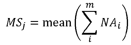 is the normalized AUCs of molecule ^^^ = 1,2,3 … ^^. In select cases, data (multi-omics, analyte, wearable, dietary intake, etc.) received from multiple subjects can be analyzed at once. The number of different subjects may vary. In some cases, the number of subjects ranges from 2 to 500, such as 3 to 250, such as 4 to 100, and including 4 to 50. In some cases, data is received from 2 or more subjects, such as 3 or more subjects, such as 4 or more subjects, such as 5 or more subjects, such as 6 or more subjects, such as 7 or more subjects, such as 8 or more subjects, such as 9 or more subjects, such as 10 or more subjects, such as 15 or more subjects, such as 20 or more subjects, such as 50 or more subjects, such as 100 or more subjects, such as 250 or more subjects and including 500 or more subjects. In such cases, methods of the invention may be performed with respect to each subject. Methods according to such embodiments may include clustering participants into different groups, e.g., to assess the molecular profile of each subject and explore the diversity in the kinetics and magnitude of the molecular responses among the different participants. Any suitable data clustering protocol may be employed. In some cases, the data clustering protocol includes consensus clustering. In embodiments, clustering includes unsupervised k-means consensus clustering. Methods according to some embodiments may additionally include fuzzy c-means clustering, which is described in Kumar, L. & E Futschik, M. (2010) Bioinformatics 26, 2841– 2848. Methods according to some embodiments may involve providing a recommendation to the subject based on the analyses discussed above. For example, embodiments include providing a recommendation to the subject based on the multi-omics analysis. Individuals who fall outside the usual molecular pattern with respect to their multi-omics data can be investigated for underlying causes for their molecular shift (medical conditions, medications or lifestyle abnormalities). Recommendations may vary and can include medication changes and lifestyle changes, and may be tailored by one of skill in the medical arts to an individual’s needs. Lifestyle changes can include, e.g., changes designed to improve the subject’s overall health, achieve weight reduction, manage a metabolic disease, reduce blood pressure, or any combination thereof. In select embodiments, methods include providing a recommendation to the subject based on the multi-omics analysis in conjunction with the wearable data discussed above.
Atty. Docket: STAN-2016WO (S22-315) Alternatively or in addition, methods may include providing a recommendation to the subject based on the multi-omics analysis in conjunction with the dietary intake data discussed above. METHODS OF GENERATING LAGGED CORRELATIONS Aspects of the invention also include methods for generating lagged correlations between first time series data and second time series data. As discussed herein, a “lagged correlation” refers to an increase or decrease in the first time series data that is in sync with the first time series data, but with a lag. For example, if " and # have a causal relationship (" causes #), # often responds to " after a certain lapse of time. Such a lapse of time is called a lag time. This means that " and # change asynchronously. An exemplary lagged correlation may involve, but is not limited to, changes in multi-omic data and changes data in data received from a wearable device (e.g., as described above). Another example involves changes in multi-omic data relative to changes in food intake data. Methods of interest include receiving first time series data and second time series data. The first and second time series day may be any suitable data that measures a variable at successive points in time. Sets of time series data may differ in the frequency with which data was sampled. Sampling frequency may depend on, e.g., the sampling modality, as different modalities may vary with respect to the feasibility of taking repeated samplings over lengths of time. In some cases, the first time series data is of a lower frequency than the second time series data. In some cases, the first time series data is internal analyte data. The “internal analyte data” may be obtained from any analyte originating internally within a subject. For example, analytes may in certain instances be found in blood, mucus, lymphatic fluid, synovial fluid, cerebrospinal fluid, saliva, bronchoalveolar lavage, amniotic fluid, amniotic cord blood, urine, vaginal fluid and semen. In addition, analytes include homogenate; isolated, purified or enriched biological particles (e.g., DNA, RNA, proteins, sub-cellular organelles, etc.); and lysates or extracts prepared from an organism or a subset of its tissues, including but not limited to, for example, plasma, serum, spinal fluid, lymph fluid, sections of the skin, respiratory, gastrointestinal, cardiovascular, and genitourinary tracts, tears, saliva, milk, blood cells, tumors, and organs. In embodiments, the internal analyte data comprises the serial levels of an internal analyte. Internal analyte data may include genomic data, epigenomic data, microbiomic data, lipidomic data, proteomic data, glycomic, transcriptomic data, metabolomic data medication data, and the like, as well as combinations thereof. In some instances, the internal analyte data is selected from the group consisting of: a protein, a lipid, a metabolite, and a medication. In some embodiments, the second time series data is wearable data. Put another way, the second time series data is wearable data that originates from a wearable device configured to collect biometric data from a subject when worn. Any suitable wearable device may be employed. The wearable device may exist currently, or is yet to be developed. Exemplary wearable devices are described above. Wearable data can include, but is not limited to, data
Atty. Docket: STAN-2016WO (S22-315) associated with body temperature, heart rate, calories burned, step count, blood pressure, release of biochemicals, physical strain, sleep and glucose levels. In certain instances, the wearable data includes sleep data, heart rate (HR) data, step count data, glucose level data, or any combination thereof. In some embodiments, the wearable data includes sleep data. In further embodiments, the wearable data includes HR data. In additional embodiments, the wearable data includes step count data. In still further embodiments, the wearable data includes glucose level data. In embodiments, at least some of the data points in the first time series data overlap with the second time series data (e.g., the data points were collected in the same or a during an overlapping timespan). To express the present this mathematically, the first time series data may be labelled as "$^% ∈ '^^, and the second time series data is labelled as #$^% ∈ '^^. If there is overlap between "$ and #$, they should satisfy the following: '^ ∩ '^ ≠ ∅ Methods of interest additionally include matching each sample point in the second time series data to sample points in the first time series data with different lagged times. In embodiments, certain events in the first time series data may be associated with certain events in the second time series data. For example, every sample point #$^ in # is used to match the sample points in "$. The shift time is labelled as '+ (set on the basis of the frequency of "$ and #$), and the matching time window is labelled as ',. So the sample points "$^ in "$ that meet the below equation are labelled as matched sample points for #$^ in #: %^ + '+ − ', ≤ %^ < %^ + '+ + ', ; ^ ∈ ^1, 2, 3 … ^^
 Then, the matched sample points "$^ are averaged as "$^ that matched with #$^ in #: $ ^
 This produces new time series data "$^% ∈ '^^. Methods of the invention additionally include calculating the Spearman correlation and P- value for each matching time-series data. Spearman’s correlation may be calculated in the conventional manner, i.e., as follows: 6 ∑ 45 ^
 Atty. Docket: STAN-2016WO (S22-315) where 1 is Spearman’s rank correlation coefficient, 4^ is the difference between the two ranks of each observation, and ^ is the number of observations. In select instances, the P-values calculated herein are Benjamini–Hochberg (BH)-adjusted P values. In embodiments, the Spearman correlation between "$ and #$ ^% ∈ '^^ is calculated with the time shift '+. The correlation 1 and P-value are then recorded as 678$9 and 1$9. As discussed above, methods include matching each sample point in the second time series data to sample points in the first time series data with different lagged times. In other words, methods include repeating the matching between each sample point in the second time series data to sample points in the first time series data, as well as the correlation calculation, with different shift times. For example, the above steps may be repeated for a series of shift times '+^, ^ = 1, 2, 3 … ^; '+: < 0 and abs('+:) = abs('+<). Then, methods may include obtaining a series 6=>$9 and a series 1$9, %+ ∈ '+. In some embodiments, methods additionally include evaluating the significance of the lagged correlation. In some such embodiments, methods include scoring correlations with similar shapes and lagged time as significant lagged correlations. Evaluating the significance of the lagged correlation may also include noting a correlation between the first time series data and the second time series data. In other words, methods according to some embodiments include inferring that biological events related to the first time series data are associated with and/or are causally related to the biological events related to the second time series data. In some embodiments, methods involve assessing the significance of the lagged correlation. In certain cases, assessing the significance of the lagged correlation includes using the Gaussian distribution to fit the 678$9 and calculating the correlations in all the shift times using the fitted Gaussian distribution, labelled as ^678$9. In some embodiments, evaluating the significance of the lagged correlation includes generating a quality score. The quality score may in some cases be indicative of the strength of the correlation. In certain versions, methods includes calculating the quality score as the absolute Spearman correlation score between ^678$9 and 678$9. In select instances, only the lagged correlation with a sufficient quality score is considered a real lagged correlation and is used for subsequent analysis. The methods described herein may be implemented as instructions run as software on one or more computer systems, and the implementation is within the capability of those skilled in the art. In particular, the computer functions for manipulations of data described herein can be developed by a programmer skilled in the art of data processing. The functions can be implemented in a number and variety of programming languages including, in some cases, mixed implementations (i.e., relying on separate portions written in more than one computing language suitably configured to communicate with one another). For example, the functions, as well as any required scripting functions, can be programmed in C, C++, Java, JavaScript, VisualBasic, Tcl/Tk, Python, Perl, Net languages such as C#, and other equivalent languages. Certain
Atty. Docket: STAN-2016WO (S22-315) mathematical functions for image processing can be written in scientific programming languages, and are preferably implemented in a form that takes advantage of a GPU. The capability of the technology is not limited by or dependent on the underlying programming language used for implementation or control of access to the basic functions. Alternatively, the functionality can be implemented from higher level functions such as toolkits that rely on previously developed functions for manipulating image data. COMPUTER-READABLE MEDIA AND DEVICES Also provided by the present disclosure are computer-readable media and devices. For example, one or more steps of any of the methods of the present disclosure (e.g., methods of generating lagged correlations, methods comprising steps of acquiring and/or analyzing proteomics data, lipidomics data, and/or metabolomics data, methods comprising steps of receiving and/or correlating wearable and/or dietary intake data, methods comprising steps of identifying causal associations, and/or the like) may be computer-implemented. By “computer- implemented” is meant at least one step of the method is implemented using one or more processors and one or more non-transitory computer-readable media. The computer- implemented methods of the present disclosure may further comprise one or more steps that are not computer-implemented, e.g., obtaining a blood microsample from a subject, performing one or more “wet lab” steps on the sample (e.g., manual extraction of proteins, lipids and/or metabolites from the sample), and/or the like. By way of example, provided are computer-implemented methods of generating lagged correlations between first time series data and second time series data, the methods being implemented using one or more processors and one or more non-transitory computer-readable media comprising instructions stored thereon, which when executed by the one or more processors, cause the one or more processors to: receive first time series data and second time series data, wherein the first time series data is of a lower frequency than the second time series data; match each sample point in the second time series data to sample points in the first time series data with different lagged times; and calculate the Spearman correlation and p-value for each matching time-series data, where correlations with similar shape and lagged time are identified as significant lagged correlations. As will be appreciated with the benefit of the present disclosure, any of the methods of the present disclosure amenable to computer-implementation may be implemented in a similar manner employing one or more processors and one or more non-transitory computer-readable media comprising instructions stored thereon, which when executed by the one or more processors, cause the one or more processors to perform one or more steps of such methods. Also provided are devices for performing any of the methods of the present disclosure. By way of example, provided are devices for generating lagged correlations between first time series data and second time series data, such devices comprising one or more processors and
Atty. Docket: STAN-2016WO (S22-315) one or more computer-readable media. The one or more computer-readable media comprise instructions stored thereon, which when executed by the one or more processors, cause the one or more processors to: receive first time series data and second time series data, wherein the first time series data is of a lower frequency than the second time series data; match each sample point in the second time series data to sample points in the first time series data with different lagged times; and calculate the Spearman correlation and p-value for each matching time-series data, where correlations with similar shape and lagged time are identified as significant lagged correlations. As will be appreciated with the benefit of the present disclosure, any of the methods of the present disclosure amenable to computer-implementation may be implemented in a similar manner by a device of the present disclosure comprising one or more processors and one or more non-transitory computer-readable media comprising instructions stored thereon, which when executed by the one or more processors, cause the one or more processors to perform one or more steps of such methods. A variety of processor-based devices may be employed to implement the embodiments of the present disclosure. Such devices may include device architecture wherein the components of the device are in electrical communication with each other using a bus. Device architecture can include a processing unit (CPU or processor), as well as a cache, that are variously coupled to the device bus. The bus couples various device components including device memory, (e.g., read only memory (ROM) and random access memory (RAM), to the processor. Device architecture can include a cache of high-speed memory connected directly with, in close proximity to, or integrated as part of the processor. Device architecture can copy data from the memory and/or the storage device to the cache for quick access by the processor. In this way, the cache can provide a performance boost that avoids processor delays while waiting for data. These and other modules can control or be configured to control the processor to perform various actions. Other device memory may be available for use as well. Memory can include multiple different types of memory with different performance characteristics. Processor can include any general purpose processor and a hardware module or software module, such as first, second and third modules stored in the storage device, configured to control the processor as well as a special-purpose processor where software instructions are incorporated into the actual processor design. The processor may essentially be a completely self-contained computing device, containing multiple cores or processors, a bus, memory controller, cache, etc. A multi-core processor may be symmetric or asymmetric. To enable user interaction with the computing device architecture, an input device can represent any number of input mechanisms, such as a microphone for speech, a touch-sensitive screen for gesture or graphical input, keyboard, mouse, motion input, speech and so forth. An output device can also be one or more of a number of output mechanisms. In some instances, multimodal devices can enable a user to provide multiple types of input to communicate with the computing device architecture. A communications interface can generally govern and manage
Atty. Docket: STAN-2016WO (S22-315) the user input and device output. There is no restriction on operating on any particular hardware arrangement and therefore the basic features here may easily be substituted for improved hardware or firmware arrangements as they are developed. The storage device is typically a non-volatile memory and can be a hard disk or other types of computer-readable media which can store data that are accessible by a computer, such as magnetic cassettes, flash memory cards, solid state memory devices, digital versatile disks, cartridges, random access memories (RAMs), read only memory (ROM), and hybrids thereof. The storage device can include software modules for controlling the processor. Other hardware or software modules are contemplated. The storage device can be connected to the device bus. In one aspect, a hardware module that performs a particular function can include the software component stored in a computer-readable medium in connection with the necessary hardware components, such as the processor, bus, output device, and so forth, to carry out various functions of the disclosed technology. Embodiments within the scope of the present disclosure may also include tangible and/or non-transitory computer-readable storage media or devices for carrying or having computer- executable instructions or data structures stored thereon. Such tangible computer-readable storage devices can be any available device that can be accessed by a general purpose or special purpose computer, including the functional design of any special purpose processor as described above. By way of example, and not limitation, such tangible computer-readable devices can include RAM, ROM, EEPROM, CD-ROM or other optical disk storage, magnetic disk storage or other magnetic storage devices, or any other device which can be used to carry or store desired program code in the form of computer-executable instructions, data structures, or processor chip design. When information or instructions are provided via a network or another communications connection (either hardwired, wireless, or combination thereof) to a computer, the computer properly views the connection as a computer-readable medium. Thus, any such connection is properly termed a computer-readable medium. Combinations of the above should also be included within the scope of the computer-readable storage devices. Computer-executable instructions include, for example, instructions and data which cause a general purpose computer, special purpose computer, or special purpose processing device to perform a certain function or group of functions. Computer-executable instructions also include program modules that are executed by computers in stand-alone or network environments. Generally, program modules include routines, programs, components, data structures, objects, and the functions inherent in the design of special-purpose processors, etc. that perform tasks or implement abstract data types. Computer-executable instructions, associated data structures, and program modules represent examples of the program code means for executing steps of the methods disclosed herein. The particular sequence of such executable instructions or associated data structures represents examples of corresponding acts for implementing the functions described in such steps.
Atty. Docket: STAN-2016WO (S22-315) Other embodiments of the disclosure may be practiced in network computing environments with many types of computer device configurations, including personal computers, hand-held devices, multi-processor devices, microprocessor-based or programmable consumer electronics, network PCs, minicomputers, mainframe computers, and the like. Embodiments may also be practiced in distributed computing environments where tasks are performed by local and remote processing devices that are linked (either by hardwired links, wireless links, or by a combination thereof) through a communications network. In a distributed computing environment, program modules may be located in both local and remote memory storage devices. For purposes of completeness, various aspects of the present disclosure are set out in the following numbered clauses. 1. A multi-omic method of analyzing a sample, the method comprising: receiving a blood microsample from a subject; extracting proteins, lipids and/or metabolites from the blood microsample; acquiring proteomics data, lipidomics data, and/or metabolomics data from the extracted proteins, lipids and/or metabolites, respectively; and analyzing the proteomics data, lipidomics data, and/or metabolomics data. 2. The method according to clause 1, wherein the blood microsample comprises 30 µl or less, 20 µl or less or 10 µl or less of blood obtained from the subject. 3. The method according to clause 1 or clause 2, wherein the blood microsample is a dried blood spot (DBS) sample produced by drying 30 µl or less, 20 µl or less or 10 µl or less of blood on a substrate. 4. The method according to any one of clauses 1 to 3, wherein the extracting comprises a biphasic extraction. 5. The method according to clause 4, wherein the biphasic extraction comprises a methyl tert-butyl ether (MTBE) extraction. 6. The method according to any one of clauses 1 to 5, wherein the acquired proteomics data is untargeted. 7. The method according to any one of clauses 1 to 5, wherein the acquired proteomics data is targeted. 8. The method according to any one of clauses 1 to 7, wherein acquiring the proteomics data comprises performing mass spectrometry on the extracted proteins. 9. The method according to any one of clauses 1 to 8, wherein the acquired metabolomics data is untargeted. 10. The method according to any one of clauses 1 to 8, wherein the acquired metabolomics data is targeted.
Atty. Docket: STAN-2016WO (S22-315) 11. The method according to any one of clauses 1 to 10, wherein acquiring the metabolomics data comprises performing mass spectrometry on the extracted metabolites. 12. The method according to any one of clauses 1 to 11, wherein the acquired lipidomics data is targeted. 13. The method according to clause 12, wherein acquiring the lipidomics data comprises performing differential mobility spectrometry (DMS) on the extracted lipids. 14. The method according to any one of clauses 1 to 13, wherein the blood microsample is a first blood microsample, and wherein the method further comprises receiving a second blood microsample from the subject, wherein the second blood microsample was acquired by the subject concurrently with the first blood microsample. 15. The method according to clause 14, comprising extracting analytes from the second blood microsample. 16. The method according to clause 15, further comprising performing a multiplexed immunoassay on the analytes extracted from the second blood microsample. 17. The method according to clause 16, wherein the multiplexed immunoassay comprises immunoassays for cytokines, cortisol, total protein, hormones, or any combination thereof. 18. The method according to any one of clauses 1 to 17, comprising determining from the blood microsample a level of a medication being taken by the subject. 19. The method according to any one of clauses 1 to 18, comprising removing from the analysis one or more analytes identified as being unstable under the conditions to which the blood microsample is subjected prior to the analysis. 20. The method according to any one of clauses 1 to 19, comprising applying a correction factor to one or more analytes identified as being unstable under the conditions to which the blood microsample is subjected prior to the analysis. 21. The method according to any one of clauses 1 to 20, comprising determining the level of a degradation product of an analyte identified as being unstable under the conditions to which the blood microsample is subjected prior to the analysis. 22. The method according to clause 21, comprising deducing the original level in the blood microsample of the analyte identified as being unstable based on the determined level of the degradation product. 23. The method according to any one of clauses 1 to 22, wherein the method is performed iteratively on time-stamped serial blood microsamples received from the subject. 24. The method according to clause 23, wherein the time-stamped serial blood microsamples were acquired by the subject one or more times within a 24 hour period.
Atty. Docket: STAN-2016WO (S22-315) 25. The method according to clause 24, wherein the time-stamped serial blood microsamples were acquired by the subject two or more, three or more, four or more, five or more, six or more, seven or more, eight or more, nine or more, or ten or more times within a 24 hour period. 26. The method according to clause 25, wherein the time-stamped serial blood microsamples were acquired for one or more, two or more, three or more, four or more, five or more, six or more, seven or more, or 14 or more consecutive 24 hour periods. 27. The method according to any one of clauses 23 to 26, further comprising receiving wearable data from the subject. 28. The method according to clause 27, wherein the wearable data comprises sleep data, heart rate (HR) data, step count data, glucose level data, or any combination thereof. 29. The method according to clause 28, wherein the glucose level data comprises continuous glucose monitoring (CGM) data. 30. The method according to any one of clauses 27 to 29, further comprising correlating the wearable data to the analyzed proteomics data, lipidomics data, and/or metabolomics data. 31. The method according to clause 30, wherein the correlating comprises identifying one or more causal associations between the wearable data and the analyzed proteomics data, lipidomics data, and/or metabolomics data. 32. The method according to any one of clauses 27 to 31, comprising receiving time-stamped medication level data from the subject, and correlating the wearable data to the time-stamped medication level data. 33. The method according to any one of clauses 1 to 32, further comprising receiving time- stamped dietary intake data from the subject. 34. The method according to clause 33, further comprising correlating the dietary intake data to the analyzed proteomics data, lipidomics data, and/or metabolomics data. 35. The method according to clause 34, wherein the correlating comprises identifying one or more causal associations between the dietary intake data and the analyzed proteomics data, lipidomics data, and/or metabolomics data. 36. The method according to any one of clauses 33 to 35, further comprising correlating the dietary intake data to the wearable data set forth in any one of clauses 27 to 29. 37. The method according to any one of clauses 30 to 36, wherein the correlating is by lagged correlation. 38. The method according to any one of clauses 1 to 37, further comprising providing a recommendation to the subject based on the multi-omics analysis.
Atty. Docket: STAN-2016WO (S22-315) 39. The method according to clause 38, further comprising providing a recommendation to the subject based on the multi-omics analysis in conjunction with the wearable data set forth in any one of clauses 27 to 29. 40. The method according to clause 38 or clause 39, further comprising providing a recommendation to the subject based on the multi-omics analysis in conjunction with the dietary intake data set forth in clause 33. 41. The method according to any one of clauses 38 to 40, wherein the recommendation to the subject is to make a lifestyle change. 42. The method according to clause 41, wherein the lifestyle change is designed to improve the subject’s overall health, achieve weight reduction, manage a metabolic disease, reduce blood pressure, or any combination thereof. 43. A method of generating lagged correlations between first time series data and second time series data, the method comprising: receiving first time series data and second time series data, wherein the first time series data is of a lower frequency than the second time series data; matching each sample point in the second time series data to sample points in the first time series data with different lagged times; and calculating the Spearman correlation and p-value for each matching time-series data, wherein correlations with similar shape and lagged time are identified as significant lagged correlations. 44. The method according to clause 43, wherein the first time series data is internal analyte data. 45. The method according to clause 44, wherein the internal analyte data comprises the serial levels of an internal analyte selected from the group consisting of: a protein, a lipid, a metabolite, and a medication. 46. The method according to any one of clauses 43 to 45, wherein the second time series data is wearable data. 47. The method according to clause 46, wherein the wearable data comprises sleep data, heart rate (HR) data, step count data, glucose level data, or any combination thereof. The following examples are offered by way of illustration and not by way of limitation. EXPERIMENTAL The discovery and profiling of blood biomarkers in a clinical or research setting is challenging due to the cost and inconvenience of in-clinic venipuncture, resulting in limited sampling frequency. In addition, current healthcare practices are reactive and based on limited
Atty. Docket: STAN-2016WO (S22-315) physiological and clinical information, often collected months or years apart. Described in the Examples below is a multi-omic microsampling approach that enables the measurement of thousands of metabolites, lipids, cytokines, and proteins in frequently-collected 10 μL blood samples in conjunction with wearable sensors. Using this approach, two case studies were conducted to (1) perform dynamic metabolic assessments of the response to a complex mixture of dietary interventions and discover highly individual-level inflammatory and metabolic responses, and (2) perform deep personal profiling to reveal large-scale dynamic molecular fluctuations as well as thousands of molecular associations including many that are associated with intraday variation in physiology (e.g., heart rate), clinical markers (glucose, cortisol), and activity. The presented methodology achieves fully remote, scalable, high-temporal-resolution omics and sensor monitoring and has the potential for comprehensive biomarker discovery and dynamic health profiling. Example 1 1. Measure a panel of metabolites (by mass spectrometry) and immune markers (by multiplexed immunoassay) before and 1-5 timepoints after a subject consumes a diet stimulus (could be a shake or other diet stimulus, e.g., suspected to be symptom- inducing for the subject due to an immune condition) a. Subtype the subject’s immune condition and predict which treatment (out of a dozen or so available) is most likely to benefit the subject. b. Optionally, use a wearable to quantify the subject’s change in heart rate and/or pulse pressure associated with consuming the diet stimulus. c. Lagged correlation between analytes/parameters may be used in analysis d. May use at-home DBS, or alternatively, at-home liquid blood sampling (rather than DBS) with a stabilizing additive. 2. Similar to #1 except the stimulus is exercise designed to cause a heart rate elevation a. Optionally diagnose a condition, including but not limited to, post-exertional malaise and predict an effective treatment (out of several available) based on the analysis. 3. Perform broad metabolomic and immune profiling at baseline (no stimulus) to identify metabolic and/or immune abnormalities, suggest interventions (drug, diet/supplement, exercise, meditation/limbic retraining, etc.) to correct abnormalities, and repeat metabolic/immune profiling at regular intervals paired with wearables to measure impact of said interventions. a. Include measurement of drug levels if intervention is a drug.
Atty. Docket: STAN-2016WO (S22-315) Example 2 – Multi-omic microsampling approach The blood microsampling and multi-omics data acquisition workflow described in the present examples are shown in FIG. 1A. The workflow comprises collecting 10 μL blood microsamples using a Mitra device, a solid matrix that collects fixed blood volumes. A wide variety of extraction conditions were tested, and a method for efficiently extracting proteins, a broad range of lipids, and metabolites from a single microsample using biphasic extraction with Methyl tert-Butyl Ether (MTBE), was developed. This extraction procedure yields an organic phase containing hydrophobic metabolites and lipids, an aqueous phase containing hydrophilic metabolites, and a methanol precipitated protein pellet processed for proteomics data acquisition. Using a separate microsample, an aqueous extraction was employed for performing multiplexed immunoassays on the Luminex platform (see Methods). Omics data sets were then processed, annotated, and curated for detailed omics analysis. To evaluate the microsampling method, the stability of proteins, metabolites, and lipids in microsamples were first examined under multiple conditions, including testing storage duration and temperature (FIG. 1b). Microsampling was then compared to conventional intravenous sampling methods (FIG.1b). Finally, two pilot case studies were performed to demonstrate how microsampling can capture important health and biological perturbations in a lifestyle context (FIG.1b). Example 3 – Protein, metabolite, and lipid stability in microsamples in multiple conditions Evaluated first was the stability of proteins, metabolites, and lipids in the blood microsamples. In brief, blood samples were collected from two participants using the 10-μL Mitra devices. A total of 36 microsamples were collected from each participant, with the microsamples stored in duplicate at 3 temperatures (4, 25, and 37 ℃) and for 5 durations at each temperature (3, 6, 24, 72, and 120 hours) before storage at -80℃ until analysis. An additional set of samples was immediately stored at - 80 ℃. Proteomics, metabolomics, and lipidomics data were acquired from the microsamples (see Methods). After quality control, imputation, and annotation of the data, there were 66 proteomics samples with 128 proteins, 71 metabolomics samples with 1,461 annotated features, and 72 lipidomics samples with 776 lipids. Each omics data set was assessed individually to examine analyte stability concerning storage duration, storage temperature, and the interaction of storage duration and temperature. The stability metrics assessed were (1) the average coefficient of variation (CV) across both participants’ samples (estimated using the formula for log-scale data12), (2) the presence of significant effects of storage conditions on analyte level using a linear regression analysis (excluding the baseline samples that were not stored at any temperature), and (3) relative importance measures (partial R2 and the Lindemann, Merenda and Gold measure, LMG1, see Methods). The results revealed that overall the majority of analytes were quite stable to storage duration, temperature, and the interaction effect (FIG.1c, d). Proteins were the most stable (CVs
Atty. Docket: STAN-2016WO (S22-315) range 0.149-1.728; median 0.397) with few 3 (2.3%), 8 (6.3%), and 6 (4.7%) associated with storage duration, temperature and the interaction effect, respectively. Metabolites were less stable (CVs range 0.054-54.328; median 0.378) with 194 (13.3%), 389 (26.6%) and 193 (13.2%) associated with storage duration, temperature and the interaction effect, respectively. Finally, lipids were the least stable (CV range 0.088-2.218 median 0.335) with 150 (19.3%), 513 (66.1%), and 172 (22.1%) associated with storage duration, temperature and the interaction effect, respectively. The relative importance models gave similar results. Thus, most analytes can be reliably measured using remote sampling, and the less stable ones can be identified and potentially measured using correction models. Example 4 – Comparison between microsample and intravenous plasma sample Examined next was the similarity between the molecular profiles derived from microsamples of whole blood compared to venipuncture plasma. Blood samples were collected from 34 participants using both microsampling and conventional intravenous blood draws (see Methods), and metabolomics and lipidomics data were acquired from each participant. The median intensity of every feature in the 34 participants was calculated separately in the two datasets, microsampling and intravenous plasma collection samples, and compared via correlation graphs (FIG. 1e). Interestingly, the results of the microsampling and intravenous collection methods were quite similar in that the Spearman correlations were 0.81 (p-value < 0.001) and 0.94 (p-value < 0.001) for 642 metabolites and 616 lipids, respectively. Metabolites and lipids that were not well correlated (Spearman correlation < 0.5) were enriched for amino acids and triglycerides (TAGs), respectively. However, most classes of molecules were very similar between the microsampling and venous blood draw, including most of the amino acids, carbohydrates, free fatty acids (FFAs), TAGs, diglycerides (DAGs), phosphatidylcholines (PCs), and other molecules. Example 5 – Case Study #1: Metabolic phenotyping responses to Ensure shake consumption As a demonstration of the power of microsampling, two case studies were performed while participants were in their native environments. The first (described in the present Example) was to examine the effect of drinking a complex mixture on metabolic profile. The second (described in the subsequent Example) was to perform very dense “24/7” profiling (98 microsamples) across periods of just greater than seven days. Individuals can differ markedly in their metabolic response to food based on their epigenomic, microbiome, metabolomic, and other factors13,14,15,16, yet the heterogeneity of this response is not well understood or fully established.
 these differences at an individual level is important in order to optimize diet and lifestyle changes for personalized health, weight reduction, and/or management of the metabolic disease. Biomarkers are typically measured at a single time point because of the difficulty of collecting high-frequency blood
Atty. Docket: STAN-2016WO (S22-315) samples using a conventional blood sampling approach, but the rapid and dynamic nature of metabolism in response to food intake requires higher resolution. To follow the diversity of metabolic responses to complex dietary mixtures, the multi-omic responses to a defined mix of carbohydrates, lipids, proteins, and micronutrients were measured. Metabolomics, lipidomics, cytokines, and hormones were analyzed in 28 participants with diverse backgrounds (FIG. 2a) and six metabolic responses metrics were developed: (1) carbohydrate, (2) lipid, (3) amino acid (protein), (4) insulin secretion, (5) free fatty acid (related to insulin sensitivity), and (6) immune (cytokines). Thirty-two participants were mailed a kit containing microsampling Mitra devices, an Ensure shake, and careful instructions for microsampling sample collection. Each participant collected one microsample (defined as 0 min), consumed the Ensure shake, and collected additional blood microsamples at 30, 60, 120, and 240 minutes after consumption (FIG. 2a). Participants returned their microsamples by overnight mail on the same day of microsample collection. The microsamples were used for multi-omics data acquisition, namely metabolomics, lipidomics, and cytokines/hormones. Four subjects without metabolomics data were removed from the dataset (see Methods, FIG. 2b). After data cleaning, curation, and annotation, 768 analytes were detected from the microsamples, including 560 metabolites, 155 lipids, and 54 cytokines/hormones for each of the 28 participants at each of the five time points (a total of 140 data points) (FIG.2b). Clustering of altered molecules Determined first was whether the microsampled multi-omics data reflected the consumption of the Ensure shake. For each time point post-consumption, the Wilcoxon rank test was utilized to define the significantly dysregulated molecules compared to time point 0 (baseline). Interestingly, the majority of significantly increased metabolites and lipids peaked at approximately 60 and 120 min, respectively, and then approached baseline levels by 240 minutes (FIG.2c). These results indicate that many molecules substantially responded to Ensure shake in the blood, and the response kinetics differed based on the classes of molecules. To quantify the molecules that shifted their levels upon Ensure shake consumption, an analysis of variance (ANOVA) test was utilized. The results show that the levels of 99 of 560 metabolites (17.7%, permutation test p-value < 0.001), 115 of 155 lipids (74.2%, permutation test p-value < 0.001), and 7 of 54 cytokines/hormones (13.0%, permutation test p-value < 0.001) significantly shifted following the Ensure shake consumption (see Methods). For the metabolites whose levels changed, the signals of analytes that differed from baseline were greater than those affected by storage duration. These results demonstrate that multi-omics analysis from microsamples can be used to measure the metabolic response to Ensure shake. The molecules significantly affected by Ensure shake were then clustered using fuzzy c- means clustering to reveal and summarize the pattern of changes associated with consumption time (see Methods). The shifted molecules were grouped into 3 major clusters across 5-time
Atty. Docket: STAN-2016WO (S22-315) points (FIG. 2d). Cluster 1 contained 39 metabolites, one lipid, and 4 cytokines that increased and then decreased with a peak at approximately 60 minutes following the Ensure shake consumption and then returned to baseline by 240 min. Cluster 2 contained 19 metabolites and 106 lipids that increased more gradually than cluster 1, peaking at approximately 60-120 minutes. Molecules in cluster 3 decreased after consuming the Ensure shake and then recovered, including 23 metabolites, 8 lipids, and 3 cytokines (FIG.2d). These results demonstrate that the molecules have different patterns and kinetics of the biochemical responses to complex mixture ingestion. Altered metabolic pathway and physiological responses to Ensure shake Explored next were the pathways and physiological responses represented by the molecules in each cluster (FIG. 2d). Cluster 1 was primarily comprised of metabolites (39 metabolites, one lipid, and 4 cytokines) and several biological pathways such as aminoacyl-tRNA biosynthesis, phenylalanine, tyrosine and tryptophan biosynthesis, and phenylalanine metabolism pathways were evident. The two major chemical classes captured in cluster 1 were amino acids and carbohydrates (FIG.2d). Both compound classes likely come directly from the Ensure shake or are metabolized quickly (FIG. 2e,f). On the other hand, for cluster 3, acetylcarnitine was the main metabolite class which dramatically decreased upon Ensure shake consumption and then recovered gradually by 240 min (FIG. 2g). This is expected because acetylcarnitine is broken down in the blood by plasma esterases to carnitine, and carnitine helps free fatty acids to be transported into the mitochondria for beta-oxidation and energy production and hence maintaining whole-body energy homeostasis17. Consistent with this interpretation, eight free fatty acids (FFAs) detected in cluster 3 decreased following the Ensure shake consumption. Notably, in cluster 2, 106 lipid species were found (FIG.2d), and most of them were triglycerides (102 TAGs with 48-52 carbons chains and 1-3 unsaturations). To better understand the molecules in the Ensure shake that might be directly detected in the participants’ microsamples, the composition of the Ensure shake was also analyzed using the same MS procedure. Nearly 50% of the compounds found in the Ensure shake can be detected in the blood, and most of the remainder were of low abundance. Importantly, of 21 high- interest metabolites that changed in the blood (FIG.2e,f,g), 17 are present in the Ensure shake. This result demonstrates that the microsampling approach is able to detect the ingested molecular signatures from blood samples. It is well known that both connecting-peptide (C-peptide) and insulin are co-secreted from the pancreas and correlate with increased carbohydrates18,19,20. As expected, the C-peptide and insulin were in the same cluster with the carbohydrates (cluster 1, FIG. 2h). Moreover, both gastric inhibitory polypeptide (GIP) and pancreatic polypeptide (PP) were found in the same cluster with insulin (cluster 1) (FIG.2h, left panel). GIP is an inhibiting hormone of the secretin family of hormones21, and its main role is stimulating insulin secretion22. Increased secretion of PP is reported to be associated with protein meal consumption, fasting, exercise, and acute
Atty. Docket: STAN-2016WO (S22-315) hypoglycemia23. In cluster 3, leptin, interferon-gamma (IFNG), and interleukin 4 (IL4) were found to decrease quickly following Ensure shake consumption (FIG. 2h, right panel). The primary function of leptin is regulating adipose tissue mass through central hypothalamus-mediated effects on hunger24; its levels are expected to decrease after food consumption. IFNG and IL4 are involved in immune responses, including allergies and antibacterial responses. Interestingly, this suggests that the Ensure shake may have anti-inflammatory properties. In summary, these results demonstrate that the kinetics of the biochemical responses, including hormones, to complex mixture ingestion can be revealed using microsampling. Metabolic phenotyping reveals unique individual responses How individuals respond to different foods is an area of great interest. The Ensure shake is a simple yet complex mixture of many types of simple molecules that can be quickly absorbed by the small intestine. To examine how different people respond to different metabolites, the diversity in the kinetics and magnitude of the molecular responses among the different participants was explored. Analysis of the samples using a t-distributed stochastic neighbor embedding (tSNE) plot shows that the samples were clustered by the participant, indicating that each participant had a unique molecular profile and that the difference between participants was greater than that of the effect of the shake. Nonetheless, a clear timewise separation of data points was observed. The study suggested that by 240 min, the metabolic levels tend to return closer to their baseline level. Unsupervised consensus clustering was then used to cluster participants into different groups. The result suggested that there were two major groups based on the molecules altered in response to the shake consumption (see Methods). In those two groups, the level of changes in metabolic features were calculated, comparing each time point to the baseline (time point 0) for each participant (see Methods). This result also suggested that participants of those two groups had different responses to the Ensure shake: Group 2 responded more slowly than the participants in Group 1, indicating the kinetics of their responses were different. Interestingly, for the thirteen individuals with a measure of insulin resistance (steady state plasma glucose (SSPG); see Methods), although statistically insignificant, a trend for IR patients to be included in Group 1 over Group 2 was observed (Wilcoxon test: p-value = 0.29). Metabolic phenotyping based on the multi-omics response to the Ensure shake Since individuals are known to vary in their response to different foods, and heterogeneity in response to the Ensure shake was found for each participant, examined next was the response of each class of molecules, carbohydrates, lipids, cytokines/hormones, and proteins to shake ingestion. A “metabolic score” was derived for the degree of an individual’s carbohydrate, lipid, FFA and protein response to the Ensure shake, along with insulin secretion and inflammatory response (cytokines) (see Methods). Briefly, for each molecule in each participant, after the Ensure shake consumption, the area under the curve (AUC) was used to represent its cumulative
Atty. Docket: STAN-2016WO (S22-315) value (FIG.3a). The AUCs of molecules for each molecular class (lipids, carbohydrates, amino acids, inflammatory molecules) were then used to calculate the response score for each participant (FIG.3b). The final metabolic scores were normalized and ranged from 0 to 1, where 0 means the lowest relative metabolic level and 1 means the highest relative metabolic level. One participant was recognized as an outlier subject and excluded during the score calculation (see Methods). For each participant, observed was a consistent distribution pattern of the molecular species within each metabolic score indicative of similar response patterns to Ensure shake consumption. However, those patterns differed greatly across subjects demonstrating high inter- individual variability in the metabolism of nutrients. The six metabolic scores were calculated for each participant. As expected, a negative correlation between FFA score and steady-state plasma glucose level (SSPG), a marker of insulin resistance25, was found. Previous studies have demonstrated that elevated plasma levels of FFA are associated with insulin resistance26. The participants were classified into five groups based on their metabolic scores using the hierarchical clustering method (FIG.3c). It was found that individuals varied considerably in their response to the shake for each of the different areas; examples selected from each of the five groups are shown in FIG. 3d. Within each group, variations were observed in the scores from the average score per metabolic class. For example, participant S30 in group 1 presented lower metabolic scores for fats and amino acids compared to the average level of the entire group. In comparison, S34 in group 5 showed higher scores for those classes (i.e., carbohydrates and amino acids) than the average scores. These differences may be due to a variety of underlying mechanisms, including levels of digestive enzymes, transporters, hormones (e.g., incretins), and/or intestinal microbes required to process particular molecules in the Ensure shake. Such underlying causes can be investigated in the future through additional analyses (such as metabolic flux analysis). Interestingly, S29 and S35 in groups 3 and 5, respectively, had higher scores in hormones and cytokines. The latter is particularly interesting as some individuals appear to have a strong inflammatory response (e.g., individual S35), whereas others have a different response to appetite-suppressing hormones. Thus, the multi- omics data from microsamples reveal the enormous heterogeneity in the biochemical responses of each individual to a complex mixture. Such information can be defined using microsampling and is important for precision nutrition diets, including inflammatory responses to food. Correlating these individual responses with medical phenotypes (e.g., LDL levels, HbA1c levels) will be important for personalized nutrition management in the future. Example 6 – Case Study #2: 24/7 personalized whole physiome profiling using wearable and multi-omics data Several studies have demonstrated that longitudinal individualized molecular profiles, clinical tests, and digital data can monitor health and enable early disease detection at an individual level 27,28,29. However, these studies use low-frequency/high-volume blood sampling
 Atty. Docket: STAN-2016WO (S22-315) (e.g., weekly or monthly), which does not enable the detection of detailed patterns such as circadian and many high-resolution lifestyle metabolic and other molecular changes. Higher frequency data collection would enable monitoring of health status as well as circadian and lifestyle patterns at high resolution in real-time, uncover relationships between molecules with each other and physiological and lifestyle activities and decipher causal associations between them at the personal level. As a proof of principle study to determine if this is feasible, explored was the combined use of the microsampling approach and wearables to explore the detailed molecular and physiological changes that occur in a real-world native context in a single individual. In this “24/7 study”, a single participant collected blood microsamples usually every one to two hours during waking hours for over seven days, with some samplings as short as 30 minutes apart (FIG.4a). A total of 98 samples were collected over seven days along with wearable data from two devices: (1) a smartwatch that recorded heart rate (HR) and step count, and (2) a continuous glucose monitor (CGM)30 (FIG.4a). Food logging was also performed many times each day using an App. The 98 microsamples were used for in-depth multi-omics profiling, including untargeted proteomics, untargeted metabolomics, targeted lipidomics, and targeted cytokine, hormone, total protein, and cortisol assays (FIG.4b, upper panel). After data acquisition and annotation, a total of 2,213 analytes were detected that included 1,051 metabolites, 811 lipids, 291 proteins, 45 cytokines, 13 metabolic panels (cytokines/hormones), 1 total protein, and 1 cortisol measurement (FIG.4b, lower panel) resulting in a total of 214,661 biochemical measurements in addition to wearable physiological data. Overall, the prospective collection of internal molecular and wearable data resulted in comprehensive, high-frequency, and abundant longitudinal data on the human whole physiome and lifestyle (FIG. 4b, c), allowing us to explore how the internal molecules and physiology change on an hourly-scale and their relationships at a personal level. To explore if multi-omic microsampling captures real biological signatures (such as food intake), two days that the participants ate high carbohydrate food (131.8 g) and low carbohydrate food (31.9 g), respectively, were selected. Then the two carbohydrate metabolites (fructose, and pyruvic acid) in microsamples were extracted and analyzed. The median values of Carbohydrate metabolites are 7.8 and 4.7, respectively, demonstrating that the omics data from microsamples roughly reflect the concentration of the food type the participants consumed. Wearable and internal multi-omics data reflect the individual physiological status Explored first was whether wearable and high-frequency internal multi-omics data can monitor and reflect the participant’s health status and searched for general patterns in the data. The 2,213 internal molecular profiles were smoothed (see Methods) and then grouped into 11 clusters using fuzzy c-means clustering analysis (FIG.4d). The two clusters followed circadian patterns. For example, cluster 4, which is enriched by a high number of metabolites, generally peaked during the day time, while cluster 11, which mostly includes lipids, peaked primarily at night (FIG.4d). Other clusters were not necessarily tied to circadian patterns and thus may reflect
Atty. Docket: STAN-2016WO (S22-315) other events. The components of the different clusters were unique, indicating that the molecules have different temporal patterns. To obtain tight and distinct molecular modules from each cluster, the community analysis method31 was used (see Methods). Interestingly, obvious peaks were found in some modules (see Methods), indicating that the molecules in modules may be triggered by specific events (FIG.4d and FIG.5a). With the detailed food (nutrition) and exercise logs, analyzed next was if and how molecular fluctuations relate to daily nutrition intake32,33 (see Methods). Briefly, nutrients in the food log were classified into several major classes based on their content level: amino acids, vitamins, fat, electrolytes, calories, carbs, and fiber. Calculated next was the association between those classes with internal molecules presented by the Jaccard index depicted in the heatmap. Interestingly, observed was a high association between classes of amino acids and fat with several modules highly enriched in amino acids, free fatty acids, and lipids, consistent with previous results34. As with the Ensure shake study, the data revealed molecular associations with daily nutrition intake. For example, the participant consumed the same meal shake every morning during the study, and a clear link was observed between daily shake consumption and temporal increase of several compounds such as 1,2,3-benzenetriol sulfate and hydroxyphenyllactic acid, which are listed as the shake’s ingredients (FIG.5a, upper panel). Cortisol is believed to follow a circadian pattern, with levels higher in the morning that decrease towards the evening35. However, events during the day related to stress, activity, and diet can impact cortisol levels36. Although morning peak levels of cortisol were evident on three days, large day-to-day variations in cortisol patterns were observed, demonstrating that within- day cortisol levels may not represent accurate inter-day cortisol patterns for this individual (FIG. 5a). This result suggests the importance of high-frequency sampling for monitoring health marker status. Importantly, this study also demonstrates the potential usage of microsamples to measure the pharmacokinetics of a drug at an individual level. The participant took a low dose of aspirin in the morning for four days. Microsampling accurately captured the pharmacokinetics of salicylic acid (hydrolyzed product of aspirin) and revealed a clearance period of about 24 hours in this person, which is similar to previous results37 (FIG. 5a, lower panel). In addition, a negative correlation was found between caffeine and sleep quality. This might be expected and has been reported in other studies38,39; however, the participant always consumed coffee before noon, indicating its long-lasting effect. Interestingly, the detailed monitoring also revealed an unidentified inflammatory event in the middle of the week, spanning 3 days, with a number of both increased inflammatory cytokines (e.g., TNFα and CD40L.) and as well as several others that decreased (e.g., Eotaxin). This event was subclinical, as no symptoms were reported, and may represent an asymptomatic infection or other stress event. Together, these results show the power of high-frequency monitoring to
Atty. Docket: STAN-2016WO (S22-315) record daily measures and health-related events not evident to the patient. The latter is particularly important for the early detection of disease40. Circadian rhythms of internal molecules in human blood Circadian rhythms are endogenous oscillators in physiological and behavioral processes over a 24-hour cycle, and they play a critical role in human health and diseases41. Circadian molecules participate in diverse physiological phenomena such as cell division, energy metabolism, and blood pressure36,42. These have not been explored at a personal level in a real- life setting because of the low frequency and high blood volume limitations of traditional blood sampling. Using the high-frequency data collected from the microsampling method, it was possible to explore and evaluate molecules associated with circadian rhythms in the human body43. Each molecule was first searched for those that exhibited a consistent pattern across all 7 days, and those that lacked a consistent daily pattern were removed (see Methods). The circadian rhythms analysis (JTK_CYCLE algorithm44) was then utilized for quantitative analysis of all the molecules (see Methods). Identified were 332 circadian molecules (Benjamini– Hochberg adjusted p-values < 0.05) that show clear circadian patterns. The circadian molecules were grouped into five major clusters using fuzzy c-means clustering. Interestingly, all clusters, except cluster 4 (enriched by protein), were dominated by lipids. The focus was on the molecules that exhibited a complete one-day cycle (those in clusters 1, 2, and 3; FIG.5b,c) and removed clusters 4 and 5, whose molecules had different levels at the beginning and end of the day. Cluster 1 was dominated by Phosphatidylcholine (PC, 32.56%) and Lysophosphatidylcholine (LPC, 25.58%), cluster 2 was dominated by Triacylglycerols (TAG, 93.65%), and cluster 3 was dominated by both TAGs (49.15%) and Phosphatidylethanolamine (PE, 22.03%) (FIG. 5d). Examples for each cluster are shown in FIG.5e. To explore the in-depth functions of the rhythmic molecules in each cluster, lipid enrichment analysis was performed using Lipid Mini-on45. LPC, PC, Sterol, and Cholesterol ester (CE) were significantly enriched in cluster 1. Previous work has shown that LPC and PC have circadian rhythms with peak concentrations in the evening, consistent with the present result46. For cluster 2, TG and Glycerolipid were significantly enriched, and for cluster 3, PE was significantly enriched. Thus, the different classes of lipids exhibit distinct circadian patterns. To explore if the circadian lipids were affected by the food intake, the food logging data was then examined. It was found that the fat nutrition intake differed across eight days, meaning that the circadian lipids are not driven by the food intake. It is plausible that circadian lipids were driven by individual rhythmic kinetics or gut microbes. In summary, multi-omics analyses from the high- frequency microsamples revealed rhythmic molecules and demonstrated that lipids related to energy metabolism have distinct circadian patterns.
Atty. Docket: STAN-2016WO (S22-315) The wearable data reflect internal molecular changes Over the past several years, longitudinal monitoring of physiological data has garnered considerable interest30,47,48,49,50. However, the ability of wearable data to predict clinical labs has been limited30. Several studies have demonstrated that wearable data can reflect and predict the internal molecules (multi-omics data), including laboratory clinic tests and metabolites on a weekly or monthly scale29,30. However, due to the low-frequency sampling of multi-omics data, the circadian patterns and causal relationships between digital and internal molecular data cannot be discerned50. The relationship between wearable data and internal molecular changes on an hourly scale at an individual level was explored, including building predictive models. Because of the different sampling frequencies of wearable and internal multi-omics data, matching the wearable and internal multi-omics data using different window sizes was first attempted. The matching windows were set as 5, 10, 20, 30, 40, 50, 60, 90, and 120 minutes. For each wearable data type (Heart rate, step count, and CGM) in the matched windows, a feature engineering pipeline30 was utilized to convert different data types into eight features (for example, the standard deviation of heart standard, maximum heart rate; see Methods) resulting in a total of 24 wearable features. The 24 wearable features were utilized to predict each analyte using the Random Forest model. Of the 2,223 molecules, 447 molecules were found to correlate with wearable features with at least one R2 > 0.3. Interestingly, also found was that most molecules have higher prediction accuracy with the larger matching window, consistent with a previous study30. Most of the 447 molecules were lipids, and enrichment analysis showed that TGs were the most predictable by wearable data. Heart rate-related features (e.g., HR range, HR maximum, and HR SD) contributed the most to the predictive models. Using the Random Forest model, it was then found that several cytokines (C-peptide, GIP, insulin, and PP) could also be predicted by wearable data. The most contributed wearable features were CGM and heart rate- related features. All those results demonstrate that wearable data could predict the high- frequency multi-omics data from microsamples. Biochemical changes in the body can occur on the order of minutes and hours51, and thus low-frequency multi-omics data (weekly or monthly) can find the associations with physiological measurements but not causal relationships29,30. Using the high-frequency microsampling approach, explored next was whether the potential causal relationships between wearable data and internal molecules could be deduced through temporal relationships; causal events are expected to precede downstream effects52. Each wearable data and molecule were first matched with different lagged times. Then, the Spearman correlation and p-value were calculated for each matching time-series data. Only the correlations with similar shapes and lagged time were scored as significant lagged correlations (see Methods). To enable this analysis, the laggedCor (lagged correlation) algorithm was developed as an R package (jaspershen.github.io/laggedcor/). This algorithm was then utilized to demonstrate that the known lagged correlation and causal relationships between step count and heart rate could be captured and quantified. Interestingly,
Atty. Docket: STAN-2016WO (S22-315) it was found a lagged correlation of 0.6 (BH adjusted p-value < 0.0001) with a shift time of -1 min (step count - heart rate), which means that one minute after the step count increases, the heart rate begins to increase. This expected result demonstrates that the lagged correlation algorithm can capture and quantify potential causal relationships. Next, a lagged correlation network between wearable and internal molecular data was generated, including 1,217 nodes (3 wearable data and 1,214 molecules) and 1,895 edges, demonstrating a high degree of association between wearable and multi-omics data. Step count and heart rate have most of the edges (57.3% and 42.6%, respectively) in the lagged correlation network. Also found was that CGM correlates more with cytokines than heart rate and step count, indicating that glucose levels strongly correlate with immune responses. This result has been demonstrated by other studies53. In addition, also observed was that step count and heart rate have many (669) overlapping correlations, as expected since they have a significant positive correlation. Interestingly, the immunity-related pathways contained some proteins that negatively correlated with CGM, which was not expected. This demonstrates the importance of following these responses at the individual level. As expected, also found was that glucagon signaling, oxidative phosphorylation pathways, and free fatty acids positively correlate with CGM. Glucagon breakdown can raise the concentration of glucose and fatty acids in the bloodstream, and oxidative phosphorylation can oxidize nutrients to release chemical energy. It was found that the caffeine metabolism pathway positively correlates with heart rate, consistent with previous studies54. Also found was that the blood coagulation pathway positively correlates with heart rate, and the neutrophil degranulation pathway negatively correlates with heart rate. These associations are believed to provide new biological insights that should be validated in future studies. Overview, these results demonstrate that the wearable data can reflect the physiological status of the participant and reveal useful insights at a personal level. The CGM glucose subnetwork was extracted from the entire lagged correlation network to further explore how glucose associates with internal molecules (FIG.6a). It was observed that CGM glucose has a significant lagged correlation with α-Synuclein (lagged correlation: 0.36, BH- adjusted p-value < 0.05) (FIG.6b), and the shift time is -55 min (α-Synuclein - CGM), indicating that α-Synuclein may directly or indirectly upregulate glucose levels in the blood. This result has been demonstrated by previous studies55,56. Previous studies have shown that higher C-peptide levels correlate with increased CGM glucose values57. The data found that CGM glucose significantly lagged correlations with C-peptide (FIG.6b) and insulin. The shift time between CGM and C-peptide in this individual is 10 minutes (lagged correlation 0.36, BH-adjusted p-values < 0.05), which means that CGM glucose precedes the concentration of C-peptide in blood by 10’. Also observed was that CGM significantly correlates with several cytokines, including TNF-β (FIG. 6b), FLT3L, IL15, IP10, and TNF-α (time shift 0 to 15 min), and four of them are proinflammatory cytokines. These results indicate that glucose can cause a rapid proinflammatory response. In summary, the results show that based on the high-frequency multi-
Atty. Docket: STAN-2016WO (S22-315) omics data from microsamples, causal associations were found between wearable and multi- omics data. The causal relationships found using the laggedcor algorithm can be validated by future experiments. Methods Sample Collection – Microsampling blood samples The Mitra device (Neoteryx, CA, USA) is used to collect the microsampling blood samples. The blood microsampling method and multi-omics data acquisition workflow were established first (FIG.1a). Developed was a method for extracting proteins, lipids, and metabolites from single microsamples, using biphasic extraction using methyl tert-butyl ether (MTBE). This extraction yields an organic phase processed for lipids, an aqueous phase processed for metabolites, and a protein pellet processed for proteomics. Using a separate microsample, an aqueous extraction for performing multiplexed immunoassays was performed on the Luminex platform. (FIG.1a). Sample Collection – Intravenous blood samples Intravenous blood from the upper forearm was drawn from overnight-fasted participants. Specimens were immediately placed on ice after collection to avoid sample deterioration. Blood was collected in a purple top tube vacutainer (BD, NJ, UCA), layered onto Ficoll media (Thermo Fisher Scientific, USA), and spun at 2,000 r.p.m. for 25 min at 24 ℃. The top layer EDTA-plasma was pipetted off, aliquoted, and immediately frozen at 80 ℃. The peripheral blood mononuclear cells (PBMC) layer was collected and counted via the cell counter, and aliquots of PBMCs were further pelleted and flash-frozen. Sample Preparation - Microsampling blood samples Mitra tip samples were thawed on ice, prepared, and analyzed randomly. Briefly, 300 μL of methanol spiked in with internal standards (provided with the Lipidyzer platform) was added to a Mitra tip and vortexed for 20 s. Lipids were solubilized by adding 1,000 μL of MTBE and incubated under agitation for 30 min at 4 °C. Phase separation was induced by the addition of 250 μL of ice-cold water. Samples were vortexed for 1 min and centrifuged at 14,000 g for 5 min at 20 °C. The upper phase containing the lipids was then collected, dried down under nitrogen, reconstituted with 200 μL of methanol, and stored at -20 °C. After biphasic extraction, the Mitra tips were resuspended in 0.1 M Tris pH 8.6 buffer, along with 10% N-octyl-glucoside and 50 mM tris(2-carboxyethyl)phosphine (TCEP), followed by shaking at 60 ℃ for 1 hour (denaturation, solubilization, and reduction). The protein mixture was subsequently alkylated with 200 mM Indole-3-acetic acid (IAA) and incubated at room temperature (24 ℃) in the dark for 30 minutes. Proteins were digested with trypsin overnight at 37 ℃ and quenched the following day with 10% (v/v) formic acid the following day. 300 μL of metabolite layer was transferred and then added 1200 uL ice-cold MeOH: Acetone: ACN (1:1:1), then vortexed for 10 s. And the sample was
Atty. Docket: STAN-2016WO (S22-315) incubated overnight at -20 ℃. The samples were vortexed for 10 s, and followed a centrifuge of 20,000 g for 10 min at 4°C. Then the sample was transferred to a new 2.0 mL tube and dried down. Finally, the samples were stored at -20 °C until data acquisition. Sample Preparation - Intravenous blood samples The sample preparation of venous blood samples for omics data acquisition is documented by Schüssler-Fiorenza Rose et al.1, Zhou et al.2, and Gao et al.29. Untargeted proteomics - Data acquisition Approximately 8 μg of tryptic digest were separated on a NanoLC 425 System (Sciex, Redwood City, CA, USA).5 μL/min flow was used with trap-elute setting using a ChromXP C18 trap column 0.5 × 10 mm, 5 μm, 120 Å (cat# 5028898, Sciex, Redwood City, CA, USA). Tryptic peptides were eluted from a ChromXP C18 column 0.3 × 150 mm, 3 μm, 120 Å (cat# 5022436, Sciex, Redwood City, CA, USA) using a 43-minute gradient from 4%–32% B with 1-hour total run. Mobile phase solvents consisted of 92.9% water, 2% acetonitrile, 5% dimethyl sulfoxide, 0.1% formic acid (A) and 92.9% acetonitrile, 2% water, 5% dimethyl sulfoxide, 0.1% formic acid (B). MS analysis was performed using Sequential Window Acquisition of all Theoretical (SWATH) acquisitions on a TripleTOF 6600 System equipped with a DuoSpray Source and 25 mm I.D. electrode (Sciex, Redwood City, CA, USA). Variable Q1 window SWATH Acquisition methods (100 windows) were built-in high sensitivity MS/MS mode with Analyst TF Software (v1.7). Untargeted proteomics - Data processing The spectra were analyzed with OpenSWATH using an in-house spectral library made from plasma and peripheral blood mononuclear cell (PBMC) samples. Peak groups were then statistically scored with the PyProphet tool (v2.0.1), and all runs were aligned using the TRIC strategy. A final data matrix was produced with 1% FDR at the peptide level and 5% FDR at the protein level. Several quality control steps were then applied to the output from SWATH2STATS. The correlation of peptide intensities between samples was calculated, and 2 samples with a mean sample correlation less than 2 SDs from the mean sample correlation were removed. An additional sample with a peptide count less than 3 SDs below the mean was removed. Poorly identified proteins and peptides were removed according to their m-scores using a target FDR of 0.05 (m-score threshold = 8.91 x 10⁻¹²). Peptides matched to an unknown protein, non-proteotypic peptides, and peptides beyond the 10 most intense peptides for a given protein were all removed. Protein intensities were then calculated by first summing the intensities of all transitions mapped to each peptide and then all peptides mapped to each protein. Proteins that were missing for > 50% of samples were removed, as were proteins whose CV among a separate set of 3 QC samples was greater than 50%. Each missing protein value was imputed using k-nearest neighbors (k = 10; using only non-imputed data; R package VIM, version 6.1.0). Protein values were then log2-transformed.
Atty. Docket: STAN-2016WO (S22-315) Untargeted metabolomics - Data acquisition Prepared samples were analyzed four times using HILIC and RPLC separation in both positive and negative ionization modes, respectively. Data were acquired on a Q Exactive Plus mass spectrometer for HILIC and a Q Exactive mass spectrometer for RPLC (Thermo Scientific, San Jose, CA, USA). Both instruments were equipped with a HESI-II probe and operated in full MS scan mode. MS/MS data were acquired on quality control samples (QC) consisting of an equimolar mixture of all samples in the study. HILIC experiments were performed using a ZIC- HILIC column 2.1 × 100 mm, 3.5 μm, 200 Å (cat# 1504470001, Millipore, Burlington, MA, USA) and mobile phase solvents consisting of 10 mM ammonium acetate in 50/50 acetonitrile/water (A) and 10 mM ammonium acetate in 95/5 acetonitrile/water (B). RPLC experiments were performed using a Zorbax SBaq column 2.1 × 50 mm, 1.7 μm, 100 Å (cat# 827700-914, Agilent Technologies, Santa Clara, CA, USA) and mobile phase solvents consisting of 0.06% acetic acid in water (A) and 0.06% acetic acid in methanol (B). Untargeted metabolomics - Data processing Data from each mode were independently analyzed using Progenesis QI software (v2.3) (Nonlinear Dynamics, Durham, NC). Metabolic features from blanks that didn’t show sufficient linearity upon dilution in QC samples (r <0.6) were discarded. To reduce metabolic features of the metabolome profile, only metabolic features present in > 2/3 of the samples were kept for further analysis. Next, in the study samples, metabolic features present in > 50% of those samples were kept for further analysis. Missing values were imputed using k-nearest neighbors (KNN) with k = 10. Data was then log2-transformed. The batch effect was evaluated using the dbnorm package61. Applying several batch removal algorithms, the ComBat model62, giving the best performance, was considered for correcting systematic variation associated with the batch. Data from each mode were independently analyzed using Progenesis QI software (v2.3, Nonlinear Dynamics). ComBat was used to do data normalization61, and KNN was used for missing value imputation. Data from each mode were merged, and metabolites were formally identified by matching fragmentation spectra and retention time to analytical-grade standards when possible or by matching experimental MS/MS to fragmentation spectra in publicly available databases using metID63. The Metabolomics Standards Initiative (MSI)64 level of confidence was used to grade metabolite annotation confidence (level 1 - level 2). Semi-targeted lipidomics - Data acquisition Prepared samples were analyzed using the Lipidyzer platform that comprises a 5500 QTRAP System equipped with a SelexION differential mobility spectrometry (DMS) interface (Sciex, Redwood City, CA, USA) and a high flow LC-30AD solvent delivery unit (Shimadzu, Kyoto, Japan). The detailed method can be found in a previous study65. In brief, lipid molecular species were identified and quantified using multiple reaction monitoring (MRM) and positive/negative ionization switching. Two acquisition methods were employed, covering 10 lipid
Atty. Docket: STAN-2016WO (S22-315) classes; method 1 had SelexION voltages turned on, while method 2 had SelexION voltages turned off. Lipidyzer data were reported by the Lipidomics Workflow Manager (LWM) software which calculates concentrations for each detected lipid as the average intensity of the analyte MRM/average intensity of the most structurally similar internal standard (IS) MRM multiplied by its concentration. Semi-targeted lipidomics - Data processing The final datasets were generated from the Lipidyzer platform, and the lipid abundances were reported as concentrations in nmol/g. Lipids detected in less than 2/3 of the samples were discarded, and missing values were imputed based on a lipid class-wise KNN-TN imputation method66. Cytokines and metabolic panel Cytokines were analyzed using the HCYTMAG-60K-PX41 kit or the HSTCMAG28SPMX13 kit. For Metabolic hormone assays, the catalog number was HMHEMAG- 34K. These assays were performed by the Human Immune Monitoring Center at Stanford University. All kits were purchased from EMD Millipore Corporation (Burlington, MA, USA) and used according to the manufacturer’s instructions with the following modifications. Briefly, samples were mixed with antibody-linked magnetic beads on a 96-well plate and incubated overnight at 4 °C with shaking. Cold (4 °C) and room temperature incubation steps were performed on an orbital shaker at 500-600 r.p.m. Plates were washed twice with wash buffer in a Biotek ELx405 washer. Following one hour of incubation at room temperature with a biotinylated detection antibody, streptavidin-PE was added for 30 minutes with shaking. Plates were washed as described, and Phosphate buffered saline (PBS) was added to wells for reading in the Luminex FlexMap3D Instrument (Thermo Fisher Scientific, USA) with a lower bound of 50 beads per sample per cytokine. Each sample was measured in a singlet. Custom Assay Chex control beads were purchased from Radix BioSolutions, Georgetown, Texas, and added to all wells. Cortisol This assay was performed by the Human Immune Monitoring Center at Stanford University using the ProcartaPlex™ Simplex Kit (Catalog number: EPX010-12190-901, ThermoFisher, Santa Clara, California, USA) and used according to the manufacturer’s instructions with modifications as described. Briefly: Beads were added to a 96-well plate and washed in a BioTek ELx405 washer. Samples were added to the plate containing the mixed antibody-linked beads, and 20 μL of the competitive conjugate was added and incubated overnight at 4 °C with shaking. Cold (4 °C) and Room temperature incubation steps were performed on an orbital shaker at 500-600 r.p.m. Following the overnight plate was washed as described, and PE was added for 30 minutes at room temperature. The plate was washed as above, and a reading buffer was added to the wells. Each sample was measured in a single well.
Atty. Docket: STAN-2016WO (S22-315) Plates were read using a Luminex FM3D FlexMap instrument with a lower bound of 50 beads per sample per cytokine. Custom Assay Chex control beads (Radix BioSolutions, Georgetown, Texas) were added to all wells. Total Protein The total protein was determined by BCA assay according to kit instructions (ThermoFisher, USA). Wearable Data The smartwatch (Fitbit) was utilized to collect the sleep, heart rate (HR), and step count data. The Fitbit Intraday API through the My Personal Health Dashboard app67 was used to retrieve sleep, HR, and step count data for the experiment period. The Dexcom G5 device was utilized to collect the continuous glucose monitoring (CGM) data. CGM data were transferred directly from the G5 device51. Dietary intake was logged manually using a notebook to track approximate meal timing and composition. Stability analysis – Study design All the microsamples were stored at -80 °C before they were prepared and analyzed. So the stability analysis was designed to explore if the molecules from the microsamples are stable in different storage conditions (temperature and duration time) before they are stored at -80 ℃. Two individuals were enrolled under the institutional review board (IRB)-approved protocol (IRB- 23602 at Stanford University) with written consent. By venipuncture, two individuals were asked to provide 10 mL of whole blood (in an EDTA purple top tube). The whole blood of each participant was poured into separate plastic reservoirs. Then 10 μL Mitra devices were touched to the surface of the blood to fill the microsample sponge. Thirty-six microsamples were generated for each participant, and microsamples were stored in duplicate at 3 temperatures (4, 25, and 37 °C) for 6 durations at the given temperature (3, 6, 24, 72, 120, and 0 hours [i.e., put into cold storage immediately]) before being stored at -80 ℃ until analysis. Then all the microsamples were prepared and used to acquire proteomics, metabolomics, and lipidomics data using the protocol described above. All the omics data were provided as Supplementary Data 1. Stability analysis – The first metric of stability After the data generation, annotation, cleaning, imputation, and transformations, each of the omic data sets (proteins, metabolite features, and lipids) were assessed for analyte stability in storage. A total of 128 proteins (n = 66 samples), 1,461 metabolites (no redundant metabolite removal, n = 71 samples), and 776 lipids (n = 72 samples) were available for the stability analysis. The first metric assessed was the coefficient of variation (CV; estimated using the formula for log-transformed data12), which was calculated separately across all of the samples for each of the two participants from whom samples were taken. The mean of the two CVs (one from each participant’s samples) was used as the CV for that analyte. The distribution of CVs was plotted.
Atty. Docket: STAN-2016WO (S22-315) Stability analysis – The second metric of stability The second stability metric was used to identify storage conditions' significant effects on the analyte level. Linear regression was performed for each analyte where the analyte level was regressed on storage duration, temperature, the duration×temperature interaction effect, and an indicator for one of the two participants (to remove the effect of the actual difference in analyte level between the participants). Since the samples that had 0 storage duration were never stored at any temperature, those samples were excluded from the analysis so that the effect of storage temperature could still be estimated, leaving 54, 59, and 60 samples for the protein, metabolite, and lipid analyses. The “lm” function in R was used, and since the objective of the study was to identify analytes that were stable under storage, a simple significance threshold of p-values = 0.05 was used to be more conservative since smaller p-value thresholds would exclude subtler potential effects of storage. The total model R2 and the partial R2 for each regression term were calculated using the “rsq” and “rsq.partial” functions of the “rsq” package (version 2.2). The Lindemann, Merenda and Gold (LMG) measure of variable importance1 was also calculated using the “calc.relimp” function of the “relaimpo” package (version 2.2-6). The proportion of statistically significant effects of storage conditions on analyte level was evaluated against the expected number of significant results at the alpha level of 0.05 to gauge the extent of signal for significant storage effects on the analytes. For each omic data set and storage condition term, the top most associated analytes (according to p-value) were plotted over time and colored by storage temperature to visually examine the identified effects. Since a lack of power might have prevented the identification of some storage effects, each regression analysis was repeated but using two separate models, one testing only storage duration and one testing only storage temperature. The benefit of this change was that the baseline samples could be included in the models testing the effect of storage duration. Comparison between microsamples and intravenous plasma To compare the microsampling and conventional intravenous plasma collection approaches, 34 participants were enrolled under the institutional review board (IRB)-approved protocol (IRB-55689 at Stanford University) with written consent. Then one microsampling blood sample and one intravenous plasma sample were collected for each participant. All the samples were immediately saved at the -80 ℃ for subsequent sample preparation. Then all the samples were prepared and used to acquire untargeted metabolomics and lipidomics data according to the above protocols. For the metabolomics data, after data processing and data curation, 22,858 metabolic features were detected (RPLC positive mode: 7,487 features, RPLC negative mode: 4,662 features, HILIC positive mode: 6,362 features, HILIC negative mode: 4,374 features). And only 642 features with annotations (MSI levels 1 & 2) remained for subsequent analysis. For the lipidomics data, 616 lipids were detected. All the omics data were provided as Supplementary Data 2.
Atty. Docket: STAN-2016WO (S22-315) Ensure shake study cohort Twenty-eight participants were enrolled in the Ensure shake study under the institutional review board (IRB)-approved protocol (IRB-47966 at Stanford University) with written consent. 21 out of 28 participants have completed demographic data. The median steady-state plasma glucose (SSPG) is 166, the median age is 64.2 years, and the median body mass index (BMI) is 29.7. Among all the participants, 38% are male, 14.3% are Asian, 14.3% are Black, 66.7% are Caucasian, and 4.8% are Hispanic. All 28 participants were mailed a kit containing microsampling devices (Mitra device), Ensure shake (contains 440 kcal, 66 g carbohydrate, 18 g protein, and 12 g fat), and instructions for the microsampling sample collection. Each participant was instructed to consume the Ensure shake and then collected microsampling blood samples immediately before consuming Ensure shake (baseline, time point 0), and at 30, 60, 120, and 240 min following Ensure shake consumption. Finally, 5 time-point microsamples were collected for each participant. Participants were asked to return their microsamples by overnight mail the same day after blood sample collection. Then all the microsamples were used for multi-omics data acquisition, namely untargeted metabolomics, targeted lipidomics, and cytokine/hormone. Four participants (S6, S26, S31, and S37) without metabolomics data were removed from the final dataset. After data cleaning, curation, and annotation, 768 analytes were detected from the microsamples, containing 560 metabolites, 155 lipids, and 54 cytokines/hormones. 24/7 study cohort Only one participant (Male, 64 years old) was enrolled in the 24/7 study under IRB- approved protocol (IRB-23602 at Stanford University) with written consent. The microsampling method enables frequent sampling on the order of minutes or hours. However, to make it acceptable and executable, the participant was instructed to perform self-collected finger prick microsamples approximately every hour during waking and every two hours overnight periods sporadically for 7 days (FIG. 4a). In addition, the participant was also instructed to leverage several wearable devices (Fitbit smartwatch, Dexcom) to acquire comprehensive digital data (wearable data), including the heart rate (HR), step count, continuous glucose monitoring (CGM), and food logging. The microsamples were immediately saved on dry ice upon collection by the participant and then shipped to the laboratory daily. Finally, 97 microsamples in total were collected. They were used to perform in-depth multi-omics data acquisition, including (1) untargeted proteomics, (2) untargeted metabolomics, (3) semi-targeted lipidomics, and (4) targeted assay (cytokine, hormones, total protein, and cortisol). After data processing, curation, and annotation, from the microsamples, a total of 2,213 analytes were finally detected that included 1,051 metabolites, 811 lipids, 291 proteins, 45 cytokines, 13 metabolic panels (cytokines/hormones), 1 total protein, and 1 cortisol.
Atty. Docket: STAN-2016WO (S22-315) General statistical, bioinformatics analysis, and data visualization Most statistical analysis and data visualization were performed using Rstudio and R language (version 4.1.2). Most of the R packages and their dependencies used in this study are maintained in CRAN (cran.r-project.org/) or Bioconductor (bioconductor.org/). The main script for analysis and data visualization was provided on GitHub (github.com/jaspershen/microsampling_multiomics). In general, before all the statistical analysis, the data are log2-transformed and then auto- scaled. All the multiple comparisons were adjusted by the Benjamini & Hochberg method (BH) using the “p.adjust” function in R. The R functions “cor” and “cor.test” were used to calculate the Spearman correlation coefficients. The R package “ggplot2” was used to perform most of the data visualization in this study. The R package “Rtsne” was used for the tSNE analysis in the Ensure shake study. The icons used in figures are from iconfont.cn which can be used for uncommercial purposes under the MIT license (pub.dev/packages/iconfont/license). Differentially expressed molecules after consuming Ensure shake In the Ensure shake study, the time point 0 (before consuming Ensure shake) was set as the baseline, and all the other 4 time points were compared to the baseline to get the differentially expressed molecules (metabolites, lipids, and cytokines/hormones). The paired Wilcoxon rank- sum test (“wilcox.test” function of R) was utilized to get the p-values. The multiple comparisons were adjusted using the Benjamini & Hochberg (BH) method (“p.adjust” function of R). And the adjusted p-values less than 0.05 were considered as significantly differentially expressed molecules. Then the number of significant molecules whose level had changed at different time points was visualized using a Sankey plot (“ggalluvial” package of R). Next, after consuming Ensure shake across all the time points, identified was the entire set of molecules whose levels changed. The ANOVA test (“anova_test” function from the “rstatix” package in R) was utilized to calculate the p-values and then adjusted using the BH method. To evaluate if the significantly expressed molecules were random or not, a permutation test was performed. In brief, the sample labels of omics data were randomly shifted to get the random datasets. Then the same method (ANOVA test) was utilized to find the altered molecules for the random dataset. This step was repeated 100 times to get a null distribution of differential molecules. Then the permutation p- value was calculated to evaluate if the expressed molecules were random. Consensus clustering In the Ensure shake study, the unsupervised K-means consensus-clustering of all samples was performed with the R packages “CancerSubtypes” and “ConsensusClusterPlus” using the significantly shifted molecules that were discovered after consuming the Ensure shake68. The data was log2-transformed first and then auto-scaled. Samples clusters were detected based on K-means clustering, Euclidean distance, and 1,000 resampling repetitions in the “ExecuteCC” function in the range of 2 to 6 clusters. The generated empirical cumulative
Atty. Docket: STAN-2016WO (S22-315) distribution function (CDF) plot initially showed the optional separation of 2 clusters for all samples. To further decide how many groups (k) should be generated, the silhouette information from clustering was extracted using the “silhouette_SimilarityMatrix function”. k = 2, 3, 4, and 5 were compared and it was found that when k = 2, high stability for clustering was obtained. And from the consensus matrix heatmaps, 2 groups seem to have the best good clustering. So finally, all the samples were assigned to 2 groups. Fuzzy c-means clustering The R package “Mfuzz” was used for fuzzy c-means clustering69. In brief, the omics data was first log2-transformed and auto-scaled, and then the minimum centroid distances were calculated for cluster numbers from 2 to 22 by step 1. The minimum centroid distance is used as the cluster validity index. Then the optimal cluster number was selected according to rule70. To get a more accurate cluster number, the clusters whose center expression data correlations are more than 0.8 were merged as one cluster. Then the optimal cluster number was used to do the fuzzy c-means clustering. For each cluster, only the molecules with memberships of more than 0.5 were retained for subsequent analysis. Metabolic scores Participant S18 was considered as an outlier in the baseline and removed from the dataset for subsequent analysis. Then 5 metabolic scores were calculated: (1) Three carbohydrates (fructose, lactic acid, and pyruvic acid) were detected and used to calculate the carbohydrate score, which represents the human’s ability to metabolize carbohydrates. (2) Nine amino acids (alloisoleucine, Alanine, isoleucine, methionine, norvaline, phenylalanine, tryptophan, tyrosine, and L-phenylalanine) were detected and used to calculate the amino acid score (protein), which represents the human’s ability to metabolize proteins. (3) 103 TAGs were detected and used to calculate the fat score, representing the human’s ability to metabolize the fat. (4) The C-peptide and insulin were detected and used to calculate the insulin secretion score, representing the human’s ability to secrete insulin. (5) The 8 free fatty acids (FFA 16:0, FFA 16:1, FFA 18:1, FFA 18:2, FFA 18:3, FFA 22:2, FFA 22:5, and FFA 22:6) were detected and used to calculate free fatty acid (insulin sensitivity) score, which represents the human’s ability to respond to insulin sensitivity. (6) All the cytokines were used to calculate the immune response score representing the human’s immune response. For each metabolic score MS, the molecules Mi (i = 1, 2, 3 … m) in this group were first defined and selected (FIG.3b), and then the dataset was log2-transformed and auto-scaled. For each participant and molecule, the intensity values across all the time points were subtracted by the baseline value, so the baseline value was 0. Then the area under the curve (AUC) Ai,j was calculated for molecule Mi (i = 1, 2, 3 … m) and participant Pj (j = 1, 2, 3 … n). To normalize the Ai,j, the Ai,j were subtracted by the minimum min(Ai,j) and divided by the range of all the AUCs
Atty. Docket: STAN-2016WO (S22-315) (max(Ai,j) - min(Ai,j)). The normalized Ai,j is labeled as NAi,j and is from 0 to 1. Then for each metabolic score MSj in each participant j, it is calculated as below: Metabolic scorej = mean(∑ ^ NAi) Where MSj is the metabolic score for participant j, and NAi is the normalized AUCs of molecule i (i = 1, 2, 3 … m). For the carbohydrate score, amino acid (protein) score, fat score, and free fatty acid score (insulin sensitivity), the high AUCs of molecules mean that the person’s ability to metabolize the molecules is low, so the final metabolic scores were calculated as 1 - MSj. For the insulin secretion score and immune response score, the final score is the same as the MSj. Enrichment analysis - Metabolomics pathway enrichment To do the metabolomics pathway enrichment, the human KEGG pathway database was downloaded from KEGG using the R package massDatabase71. The original KEGG database has 275 metabolic pathways. These were then separated them into metabolic pathways or disease pathways based on the “Class” information for each pathway. The pathways with the “Human Disease'' class were assigned to the disease pathway database, which contains 74 pathways, and remained 201 pathways were assigned to the metabolic pathway database. The pathway enrichment analysis is used in the Hypergeometric distribution test from the tidyMass project72. The BH method was used to adjust p-values, and the cutoff was set as 0.05 (BH- adjusted p-values < 0.05). Enrichment analysis - Lipidomics data enrichment analysis The Lipid Mini-on software was utilized to do the lipid enrichment analysis45. In brief, the lipids’ names were first modified to meet the requirement of the tool. The dysregulated lipids were uploaded as query files, and all the detected lipids were uploaded as universe files. The default Fisher’s exact test was used as the enrichment test method. The category, main class, subclass, individual chains, individual chain length, and number of double bonds were selected for general parameters to test. Finally, the enrichment result containing detailed tables and networks was downloaded for subsequent analysis. Enrichment analysis - Proteomics pathway enrichment The R package “clusterProfiler” was utilized for proteomics pathway enrichment. First, the gene ID of proteins to ENTREZID ID were converted, and then the GO database was utilized for GO term enrichment analysis. The p-values were adjusted using the BH method, and the cutoff was set as 0.05. Only the enriched GO terms with at least mapped 5 proteins remained to ensure that the enriched GO terms have enough genes. To reduce the redundancy of enriched GO terms, the similarity between GO terms was calculated using the “Wang” algorithm from the R package “simplifyEnrichment”73. And only the connections with similarities > 0.3 remained to construct the GO term similarity network. Then the community analysis (R package “igraph”) was
Atty. Docket: STAN-2016WO (S22-315) utilized to divide this network into different modules. The GO term with the smaller enrichment adjusted p-values was selected for each module as the representative. LOESS smoothing data In the 24/7 study, the time points of microsamples for each day differ. However, the circadian analysis requires enough time points for each day. So the locally estimated scatterplot smoothing (LOESS) method was leveraged to smooth and predict the multi-omics data in the specific time points (every half hour) described in another publication74. In brief, for each molecule, it was fitted with the LOESS regression method for each day (“loess” function in R). During the fitting, LOESS's argument “span” was optimized by cross-validation. As the gap between two days is always more than 4 hours, the time between two days was not fitted for an accurate and robust fitting and prediction. After getting the LOESS prediction model, each molecule's intensity was predicted every half hour during the days. Correlation network and community analysis In the 24/7 study, a correlation network was constructed for each cluster obtained using fuzzy c-means clustering. In brief, the Spearman correlation was calculated for every two molecules. Only the correlations with coefficient > 0.7 and BH adjusted p-values < 0.05 remained for subsequent analysis. All the remained correlations were used to construct the correlation network. To get more accurate and distinct modules, the community analysis was used to extract subnetworks (modules) from the correlation network31. Here, the fast greedy modularity optimization algorithm (“cluster_fast_greedy” function from the R package “igraph”) was used. Finally, 11 clusters and 83 modules were detected. The R packages “igraph” and “ggraph” were used to visualize the network. Associations between molecular modules and nutrition intake In the 24/7 study, to evaluate the associations between molecular modules and nutrition intake, peak detection (Gaussian distribution fitting) was first utilized to find the “peaks” in each module. If there is a peak, then it is marked as “1” at this time. If not, it is marked as “0”. For food, if the participant consumes this food at this time point, then this time point will be marked as “1” for this food. And then, for each food and module, the Jaccard index was calculated, and only the pairs with a Jaccard index > 0.3 were retained for subsequent analysis. Consistency score for molecules In the 24/7 study, the consistency score was designed and calculated for each molecule to assess if one molecule is consistent daily. LOESS smoothed data was used for consistency score calculation. For each molecule, the Spearman correlations between two days were calculated, and the median correlation value was calculated and considered as the consistency score for this molecule. Only the molecules with consistency scores > 0.6 were retained for the next circadian analysis.
Atty. Docket: STAN-2016WO (S22-315) Circadian rhythm analysis In the 24/7 study, the R package “MetaCycle” is used to do the circadian rhythm analysis43. The LOESS smoothed omics data were log2-transformed and auto-scaled. And then, the times for samples were set as the time points in the “meta2d” function. The Lomb-Scargle was selected for circadian rhythm analysis75. The p-values were adjusted using the BH method. Only the molecules with BH-adjusted p-values < 0.05 were considered statistically significant circadian molecules and retained for subsequent analysis. Wearable data predicts internal molecules In the 24/7 study, to evaluate if the wearable data could be utilized to predict internal molecules, the method from a previous publishment30 was used. Because the frequency of wearable data and internal molecules are different, it was necessary to match the internal molecule and wearable data first. The matching windows were set as 5, 10, 20, 30, 40, 50, 60, 90, and 120 mins, respectively. And for the wearable data points that matched with internal molecules, a feature engineering pipeline30 was utilized to convert the wearable data into eight features: mean value, median value, standard, maximum, minimum, skewness, kurtosis, and range. So for each wearable data, it was converted into 8 features. The wearable data (heart rate, step count, and CGM) were converted to 24 features in total and were used as independent variables to predict each internal molecule. The random forest model (R package “caret” and “RandomForest”), which has been proven to have the best prediction accuracy, was utilized30. The 24 wearable features were combined for each internal molecule to construct the prediction model. The 7-fold cross-validation method was used during the prediction model construction. The importance of each wearable feature was saved for subsequent analysis. Lagged correlation In the 24/7 study, to calculate the lagged correlation between wearable data and internal molecules, the laggedCor algorithm (lagged correlation) and an R package named “laggedcor” were developed (jaspershen.github.io/laggedcor/). The laggedCor algorithm can be used to extract potential causal relationships. Let’s assume that X is wearable data and Y is internal omics data. In a real biological system, if X and Y have a causal relationship (X causes Y), Y often responds to X after a certain lapse of time. Such a lapse of time is called a lag time. So it means that X and Y change asynchronously. To explore if X and Y have a potential causal relationship, shifted is the lag time between X and Y for matching and then the correlation between them is calculated. Suppose the X and Y have a potential causal relationship and the lag time is T, then the highest lagged correlation between X and Y at the lag time T is obtained. Briefly, two time-series data are used as the inputs for laggedcor. The lower frequency time-series data (in the 24/7 study is the omics data) is labeled as Xt (t ∈ Ti), and the higher frequency time-series data (in the 24/7 study is the wearable data) is labeled as Yt (t ∈ Tj). To make sure that there are overlaps between Xti and Ytj, they should meet the below equation:
Atty. Docket: STAN-2016WO (S22-315) Ti ∩ Tj ≠ ∅ then the two series data, Xt and Yt are used to calculate the lagged correlation as described below steps. Step 1: Matching between Xt and Yt. Every sample point Ytj in Y is used to match the sample points in Xt. The shift time is labeled as Ts (Ts is set based on the frequency of Xt and Yt), and the matching time window is labeled as Tw. So the sample points Xti in Xt that meet the below equitation are labeled as matched sample points for Ytj in Y. tj + Ts - @A ≤ ti<tj @A 5 + Ts + 5 ; i ∈ (1, 2, 3 … m) The the with Ytj in Y.
 $^ Obtained then is the new time-series data Xt (t ∈ Tj). Step 2: Correlation calculation. Then the Spearman correlation between Xt and Yt (t ∈ Tj) is calculated with the shift time Ts. And the correlation rho and p-value are recorded as Corts and pts. Step 3: Repeat step 1 and step 2 with different shift time. Then, step 1 and step 2 are repeated for a series shift times Tsi, i = 1, 2, 3 … n; Ts1 < 0 and abs(Ts1) = abs(Tsn). Obtained then is a series Corts and a series pts, ts ∈ Tsi. Step 4: Evaluation of the significance of lagged correlation. The max correlation of Corts and related p-value are extracted as the lagged correlation for time-series data Xt and Yt. To evaluate if the lagged correlation is significant, the Gaussian distribution is used to fit the Corts, and the correlations in all the shift times are calculated using the fitted Gaussian distribution and labeled as PCorts. The quality score was then calculated as the absolute Spearman correlation score between PCorts and Corts. Only the lagged correlation with a quality score was considered a real lagged correlation and used for subsequent analysis. References 1. Schüssler-Fiorenza Rose, S. M. et al. A longitudinal big data approach for precision health. Nat. Med.25, 792–804 (2019). 2. Zhou, W. et al. Longitudinal multi-omics of host-microbe dynamics in prediabetes. Nature 569, 663–671 (2019). 3. Guthrie, R. & Susi, A. A SIMPLE PHENYLALANINE METHOD FOR DETECTING PHENYLKETONURIA IN LARGE POPULATIONS OF NEWBORN INFANTS. Pediatrics 32, 338–343 (1963). 4. Antunes, M. V., Charão, M. F. & Linden, R. Dried blood spots analysis with mass spectrometry: Potentials and pitfalls in therapeutic drug monitoring. Clin. Biochem.49, 1035–1046 (2016). 5. Corso, G., D’Apolito, O., Gelzo, M., Paglia, G. & Dello Russo, A. A powerful couple in the future of clinical biochemistry: in situ analysis of dried blood spots by ambient mass spectrometry. Bioanalysis 2,
Atty. Docket: STAN-2016WO (S22-315) 1883–1891 (2010). 6. Bennett, M. J. et al. Newborn screening for metabolic disorders: how are we doing, and where are we going? Clin. Chem.58, 324–331 (2012). 7. Volani, C. et al. Pre-analytic evaluation of volumetric absorptive microsampling and integration in a mass spectrometry-based metabolomics workflow. Anal. Bioanal. Chem.409, 6263–6276 (2017). 8. van den Broek, I. et al. Application of volumetric absorptive microsampling for robust, high- throughput mass spectrometric quantification of circulating protein biomarkers. Clinical Mass Spectrometry vols 4-525–33 Preprint at https://doi.org/10.1016/j.clinms.2017.08.004 (2017). 9. Molloy, M. P. et al. Proteomic Analysis of Whole Blood Using Volumetric Absorptive Microsampling for Precision Medicine Biomarker Studies. J. Proteome Res.21, 1196–1203 (2022). 10. Lei, B. U. W. & Prow, T. W. A review of microsampling techniques and their social impact. Biomed. Microdevices 21, 81 (2019). 11. Zhuang, Y.-J., Mangwiro, Y., Wake, M., Saffery, R. & Greaves, R. F. Multi-omics analysis from archival neonatal dried blood spots: limitations and opportunities. Clin. Chem. Lab. Med. (2022) doi:10.1515/cclm-2022-0311. 12. Canchola, J. A. Correct Use of Percent Coefficient of Variation (%CV) Formula for Log- Transformed Data. MOJ Proteomics & Bioinformatics vol. 6 Preprint at https://doi.org/10.15406/mojpb.2017.06.00200 (2017). 13. Hannon, B. A. et al. Single Nucleotide Polymorphisms Related to Lipoprotein Metabolism Are Associated with Blood Lipid Changes following Regular Avocado Intake in a Randomized Control Trial among Adults with Overweight and Obesity. The Journal of Nutrition vol. 1501379–1387 Preprint at https://doi.org/10.1093/jn/nxaa054 (2020). 14. Berry, S. E. et al. Human postprandial responses to food and potential for precision nutrition. Nat. Med.26, 964–973 (2020). 15. Wang, D. D. et al. The gut microbiome modulates the protective association between a Mediterranean diet and cardiometabolic disease risk. Nat. Med.27, 333–343 (2021). 16. Turnbaugh, P. J. et al. The effect of diet on the human gut microbiome: a metagenomic analysis in humanized gnotobiotic mice. Sci. Transl. Med.1, 6ra14 (2009). 17. Spiekerkoetter, U. Mitochondrial fatty acid oxidation disorders: clinical presentation of long-chain fatty acid oxidation defects before and after newborn screening. Journal of Inherited Metabolic Disease vol.33527–532 Preprint at https://doi.org/10.1007/s10545-010-9090-x (2010). 18. Gannon, M. C., Nuttall, F. Q., Westphal, S. A. & Seaquist, E. R. The effect of fat and carbohydrate on plasma glucose, insulin, C-peptide, and triglycerides in normal male subjects. J. Am. Coll. Nutr.12, 36– 41 (1993). 19. Ludwig, D. S. et al. The carbohydrate-insulin model: a physiological perspective on the obesity pandemic. The American Journal of Clinical Nutrition vol. 114 1873–1885 Preprint at https://doi.org/10.1093/ajcn/nqab270 (2021). 20. Hall, K. D. A review of the carbohydrate–insulin model of obesity. European Journal of Clinical Nutrition vol.71323–326 Preprint at https://doi.org/10.1038/ejcn.2016.260 (2017). 21. Meier, J. J. & Nauck, M. A. Glucagon-like peptide 1(GLP-1) in biology and pathology.
Atty. Docket: STAN-2016WO (S22-315) Diabetes/Metabolism Research and Reviews vol.2191–117 Preprint at https://doi.org/10.1002/dmrr.538 (2005). 22. Pederson, R. A. & McIntosh, C. H. S. Discovery of gastric inhibitory polypeptide and its subsequent fate: Personal reflections. Journal of Diabetes Investigation vol. 7 4–7 Preprint at https://doi.org/10.1111/jdi.12480 (2016). 23. Katsuura, G., Asakawa, A. & Inui, A. Roles of pancreatic polypeptide in regulation of food intake. Peptides vol.23323–329 Preprint at https://doi.org/10.1016/s0196-9781(01)00604-0 (2002). 24. Kelesidis, T., Kelesidis, I., Chou, S. & Mantzoros, C. S. Narrative review: the role of leptin in human physiology: emerging clinical applications. Ann. Intern. Med.152, 93–100 (2010). 25. Kim, S. H. & Reaven, G. M. Insulin Resistance and Hyperinsulinemia. Diabetes Care vol.311433– 1438 Preprint at https://doi.org/10.2337/dc08-0045 (2008). 26. Xin, Y. et al. Elevated free fatty acid level is associated with insulin-resistant state in nondiabetic Chinese people. Diabetes Metab. Syndr. Obes.12, 139–147 (2019). 27. Chen, R. et al. Personal omics profiling reveals dynamic molecular and medical phenotypes. Cell 148, 1293–1307 (2012). 28. Piening, B. D. et al. Integrative Personal Omics Profiles during Periods of Weight Gain and Loss. Cell Systems vol.6157–170.e8 Preprint at https://doi.org/10.1016/j.cels.2017.12.013 (2018). 29. Gao, P. et al. Precision environmental health monitoring by longitudinal exposome and multi-omics profiling. Genome Res.32, 1199–1214 (2022). 30. Dunn, J. et al. Wearable sensors enable personalized predictions of clinical laboratory measurements. Nat. Med.27, 1105–1112 (2021). 31. Price, N. D. et al. A wellness study of 108 individuals using personal, dense, dynamic data clouds. Nat. Biotechnol.35, 747–756 (2017). 32. Burton-Pimentel, K. J. et al. Discriminating Dietary Responses by Combining Transcriptomics and Metabolomics Data in Nutrition Intervention Studies. Mol. Nutr. Food Res.65, e2000647 (2021). 33. Contrepois, K. et al. Molecular Choreography of Acute Exercise. Cell 181, 1112–1130.e16 (2020). 34. DiNicolantonio, J. J. & O’Keefe, J. H. Effects of dietary fats on blood lipids: a review of direct comparison trials. Open Heart 5, e000871 (2018). 35. Mohd Azmi, N. A. S. et al. Cortisol on Circadian Rhythm and Its Effect on Cardiovascular System. Int. J. Environ. Res. Public Health 18, (2021). 36. Stachowicz, M. & Lebiedzińska, A. The effect of diet components on the level of cortisol. European Food Research and Technology vol.2422001–2009 Preprint at https://doi.org/10.1007/s00217-016-2772- 3 (2016). 37. Cao, W. et al. Drug-drug interactions between salvianolate injection and aspirin based on their metabolic enzymes. Biomed. Pharmacother.135, 111203 (2021). 38. Watson, E. J., Coates, A. M., Kohler, M. & Banks, S. Caffeine Consumption and Sleep Quality in Australian Adults. Nutrients 8, (2016). 39. Clark, I. & Landolt, H. P. Coffee, caffeine, and sleep: A systematic review of epidemiological studies and randomized controlled trials. Sleep Med. Rev.31, 70–78 (2017). 40. Li, X. et al. Digital Health: Tracking Physiomes and Activity Using Wearable Biosensors Reveals
Atty. Docket: STAN-2016WO (S22-315) Useful Health-Related Information. PLoS Biol.15, e2001402 (2017). 41. Fishbein, A. B., Knutson, K. L. & Zee, P. C. Circadian disruption and human health. Journal of Clinical Investigation vol.131 Preprint at https://doi.org/10.1172/jci148286 (2021). 42. Patke, A., Young, M. W. & Axelrod, S. Molecular mechanisms and physiological importance of circadian rhythms. Nat. Rev. Mol. Cell Biol.21, 67–84 (2020). 43. Wu, G., Anafi, R. C., Hughes, M. E., Kornacker, K. & Hogenesch, J. B. MetaCycle: an integrated R package to evaluate periodicity in large scale data. Bioinformatics 32, 3351–3353 (2016). 44. Hughes, M. E., Hogenesch, J. B. & Kornacker, K. JTK_CYCLE: An Efficient Nonparametric Algorithm for Detecting Rhythmic Components in Genome-Scale Data Sets. Journal of Biological Rhythms vol.25372–380 Preprint at https://doi.org/10.1177/0748730410379711 (2010). 45. Clair, G. et al. Lipid Mini-On: mining and ontology tool for enrichment analysis of lipidomic data. Bioinformatics 35, 4507–4508 (2019). 46. Chua, E. C.-P. et al. Extensive diversity in circadian regulation of plasma lipids and evidence for different circadian metabolic phenotypes in humans. Proc. Natl. Acad. Sci. U. S. A.110, 14468–14473 (2013). 47. Alavi, A. et al. Real-time alerting system for COVID-19 and other stress events using wearable data. Nat. Med.28, 175–184 (2022). 48. Mishra, T. et al. Pre-symptomatic detection of COVID-19 from smartwatch data. Nature Biomedical Engineering 4, 1208–1220 (2020). 49. Marabita, F. et al. Multiomics and digital monitoring during lifestyle changes reveal independent dimensions of human biology and health. Cell Syst 13, 241–255.e7 (2022). 50. Miller, I. J. et al. Real-time health monitoring through urine metabolomics. NPJ Digit Med 2, 109 (2019). 51. Hall, H. et al. Glucotypes reveal new patterns of glucose dysregulation. PLoS Biol.16, e2005143 (2018). 52. Bizzarri, M. et al. A call for a better understanding of causation in cell biology. Nat. Rev. Mol. Cell Biol.20, 261–262 (2019). 53. Shomali, N. et al. Harmful effects of high amounts of glucose on the immune system: An updated review. Biotechnol. Appl. Biochem.68, 404–410 (2021). 54. Bitar, A., Mastouri, R. & Kreutz, R. P. Caffeine Consumption and Heart Rate and Blood Pressure Response to Regadenoson. PLoS One 10, e0130487 (2015). 55. Rodriguez-Araujo, G. et al. Alpha-synuclein elicits glucose uptake and utilization in adipocytes through the Gab1/PI3K/Akt transduction pathway. Cell. Mol. Life Sci.70, 1123–1133 (2013). 56. Wijesekara, N. et al. α-Synuclein Regulates Peripheral Insulin Secretion and Glucose Transport. Front. Aging Neurosci.13, 665348 (2021). 57. Buckingham, B. et al. CGM-measured glucose values have a strong correlation with C-peptide, HbA1c and IDAAC, but do poorly in predicting C-peptide levels in the two years following onset of diabetes. Diabetologia 58, 1167–1174 (2015). 58. Paniagua-González, L. et al. Comparison of conventional dried blood spots and volumetric absorptive microsampling for tacrolimus and mycophenolic acid determination. J. Pharm. Biomed. Anal.
Atty. Docket: STAN-2016WO (S22-315) 208, 114443 (2022). 59. Andersen, I. K. L., Rosting, C., Gjelstad, A. & Halvorsen, T. G. Volumetric absorptive MicroSampling vs. other blood sampling materials in LC–MS-based protein analysis – preliminary investigations. Journal of Pharmaceutical and Biomedical Analysis vol. 156 239–246 Preprint at https://doi.org/10.1016/j.jpba.2018.04.036 (2018). 60. Lancaster, S. M. et al. Global, distinctive, and personal changes in molecular and microbial profiles by specific fibers in humans. Cell Host Microbe 30, 848–862.e7 (2022). 61. Bararpour, N. et al. DBnorm as an R package for the comparison and selection of appropriate statistical methods for batch effect correction in metabolomic studies. Scientific Reports vol.11 Preprint at https://doi.org/10.1038/s41598-021-84824-3 (2021). 62. Johnson, W. E., Li, C. & Rabinovic, A. Adjusting batch effects in microarray expression data using empirical Bayes methods. Biostatistics 8, 118–127 (2007). 63. Shen, X. et al. metID: an R package for automatable compound annotation for LC−MS-based data. Bioinformatics vol.38568–569 Preprint at https://doi.org/10.1093/bioinformatics/btab583 (2022). 64. Sumner, L. W. et al. Proposed minimum reporting standards for chemical analysis. Metabolomics vol.3211–221 Preprint at https://doi.org/10.1007/s11306-007-0082-2 (2007). 65. Contrepois, K. et al. Cross-Platform Comparison of Untargeted and Targeted Lipidomics Approaches on Aging Mouse Plasma. Sci. Rep.8, 17747 (2018). 66. Shah, J. S. et al. Distribution based nearest neighbor imputation for truncated high dimensional data with applications to pre-clinical and clinical metabolomics studies. BMC Bioinformatics 18, 114 (2017). 67. Bahmani, A. et al. A scalable, secure, and interoperable platform for deep data-driven health management. Nat. Commun.12, 5757 (2021). 68. Xu, T. et al. CancerSubtypes: an R/Bioconductor package for molecular cancer subtype identification, validation and visualization. Bioinformatics vol. 33 3131–3133 Preprint at https://doi.org/10.1093/bioinformatics/btx378 (2017). 69. Kumar, L. & E Futschik, M. Mfuzz: a software package for soft clustering of microarray data. Bioinformation 2, 5–7 (2007). 70. Schwämmle, V. & Jensen, O. N. A simple and fast method to determine the parameters for fuzzy c-means cluster analysis. Bioinformatics 26, 2841–2848 (2010). 71. Shen, X., Wang, C. & Snyder, M. P. massDatabase: utilities for the operation of the public compound and pathway database. Bioinformatics 38, 4650–4651 (2022). 72. Shen, X. et al. TidyMass an object-oriented reproducible analysis framework for LC-MS data. Nat. Commun.13, 4365 (2022). 73. Gu, Z. & Hübschmann, D. simplifyEnrichment: an R/Bioconductor package for Clustering and Visualizing Functional Enrichment Results. Preprint at https://doi.org/10.1101/2020.10.27.312116. 74. Lehallier, B. et al. Undulating changes in human plasma proteome profiles across the lifespan. Nat. Med.25, 1843–1850 (2019). 75. Glynn, E. F., Chen, J. & Mushegian, A. R. Detecting periodic patterns in unevenly spaced gene expression time series using Lomb-Scargle periodograms. Bioinformatics 22, 310–316 (2006).
Atty. Docket: STAN-2016WO (S22-315) Accordingly, the preceding merely illustrates the principles of the present disclosure. It will be appreciated that those skilled in the art will be able to devise various arrangements which, although not explicitly described or shown herein, embody the principles of the invention and are included within its spirit and scope. Furthermore, all examples and conditional language recited herein are principally intended to aid the reader in understanding the principles of the invention and the concepts contributed by the inventors to furthering the art, and are to be construed as being without limitation to such specifically recited examples and conditions. Moreover, all statements herein reciting principles, aspects, and embodiments of the invention as well as specific examples thereof, are intended to encompass both structural and functional equivalents thereof. Additionally, it is intended that such equivalents include both currently known equivalents and equivalents developed in the future, i.e., any elements developed that perform the same function, regardless of structure. The scope of the present invention, therefore, is not intended to be limited to the exemplary embodiments shown and described herein.
Claims
Atty. Docket: STAN-2016WO (S22-315) WHAT IS CLAIMED IS: 1. A multi-omic method of analyzing a sample, the method comprising: receiving a blood microsample from a subject; extracting proteins, lipids and/or metabolites from the blood microsample; acquiring proteomics data, lipidomics data, and/or metabolomics data from the extracted proteins, lipids and/or metabolites, respectively; and analyzing the proteomics data, lipidomics data, and/or metabolomics data. 2. The method according to claim 1, wherein the blood microsample comprises 30 µl or less, 20 µl or less or 10 µl or less of blood obtained from the subject. 3. The method according to claim 1 or claim 2, wherein the blood microsample is a dried blood spot (DBS) sample produced by drying 30 µl or less, 20 µl or less or 10 µl or less of blood on a substrate. 4. The method according to any one of claims 1 to 3, wherein the extracting comprises a biphasic extraction. 5. The method according to claim 4, wherein the biphasic extraction comprises a methyl tert-butyl ether (MTBE) extraction. 6. The method according to any one of claims 1 to 5, wherein the acquired proteomics data is untargeted. 7. The method according to any one of claims 1 to 5, wherein the acquired proteomics data is targeted. 8. The method according to any one of claims 1 to 7, wherein acquiring the proteomics data comprises performing mass spectrometry on the extracted proteins. 9. The method according to any one of claims 1 to 8, wherein the acquired metabolomics data is untargeted. 10. The method according to any one of claims 1 to 8, wherein the acquired metabolomics data is targeted.
Atty. Docket: STAN-2016WO (S22-315) 11. The method according to any one of claims 1 to 10, wherein acquiring the metabolomics data comprises performing mass spectrometry on the extracted metabolites. 12. The method according to any one of claims 1 to 11, wherein the acquired lipidomics data is targeted. 13. The method according to claim 12, wherein acquiring the lipidomics data comprises performing differential mobility spectrometry (DMS) on the extracted lipids. 14. The method according to any one of claims 1 to 13, wherein the blood microsample is a first blood microsample, and wherein the method further comprises receiving a second blood microsample from the subject, wherein the second blood microsample was acquired by the subject concurrently with the first blood microsample. 15. The method according to claim 14, comprising extracting analytes from the second blood microsample. 16. The method according to claim 15, further comprising performing a multiplexed immunoassay on the analytes extracted from the second blood microsample. 17. The method according to claim 16, wherein the multiplexed immunoassay comprises immunoassays for cytokines, cortisol, total protein, hormones, or any combination thereof. 18. The method according to any one of claims 1 to 17, comprising determining from the blood microsample a level of a medication being taken by the subject. 19. The method according to any one of claims 1 to 18, comprising removing from the analysis one or more analytes identified as being unstable under the conditions to which the blood microsample is subjected prior to the analysis. 20. The method according to any one of claims 1 to 19, comprising applying a correction factor to one or more analytes identified as being unstable under the conditions to which the blood microsample is subjected prior to the analysis. 21. The method according to any one of claims 1 to 20, comprising determining the level of a degradation product of an analyte identified as being unstable under the conditions to which the blood microsample is subjected prior to the analysis.
Atty. Docket: STAN-2016WO (S22-315) 22. The method according to claim 21, comprising deducing the original level in the blood microsample of the analyte identified as being unstable based on the determined level of the degradation product. 23. The method according to any one of claims 1 to 22, wherein the method is performed iteratively on time-stamped serial blood microsamples received from the subject. 24. The method according to claim 23, wherein the time-stamped serial blood microsamples were acquired by the subject one or more times within a 24 hour period. 25. The method according to claim 24, wherein the time-stamped serial blood microsamples were acquired by the subject two or more, three or more, four or more, five or more, six or more, seven or more, eight or more, nine or more, or ten or more times within a 24 hour period. 26. The method according to claim 25, wherein the time-stamped serial blood microsamples were acquired for one or more, two or more, three or more, four or more, five or more, six or more, seven or more, or 14 or more consecutive 24 hour periods. 27. The method according to any one of claims 23 to 26, further comprising receiving wearable data from the subject. 28. The method according to claim 27, wherein the wearable data comprises sleep data, heart rate (HR) data, step count data, glucose level data, or any combination thereof. 29. The method according to claim 28, wherein the glucose level data comprises continuous glucose monitoring (CGM) data. 30. The method according to any one of claims 27 to 29, further comprising correlating the wearable data to the analyzed proteomics data, lipidomics data, and/or metabolomics data. 31. The method according to claim 30, wherein the correlating comprises identifying one or more causal associations between the wearable data and the analyzed proteomics data, lipidomics data, and/or metabolomics data. 32. The method according to any one of claims 27 to 31, comprising receiving time-stamped medication level data from the subject, and correlating the wearable data to the time-stamped medication level data.
Atty. Docket: STAN-2016WO (S22-315) 33. The method according to any one of claims 1 to 32, further comprising receiving time- stamped dietary intake data from the subject. 34. The method according to claim 33, further comprising correlating the dietary intake data to the analyzed proteomics data, lipidomics data, and/or metabolomics data. 35. The method according to claim 34, wherein the correlating comprises identifying one or more causal associations between the dietary intake data and the analyzed proteomics data, lipidomics data, and/or metabolomics data. 36. The method according to any one of claims 33 to 35, further comprising correlating the dietary intake data to the wearable data set forth in any one of claims 27 to 29. 37. The method according to any one of claims 30 to 36, wherein the correlating is by lagged correlation. 38. The method according to any one of claims 1 to 37, further comprising providing a recommendation to the subject based on the multi-omics analysis. 39. The method according to claim 38, further comprising providing a recommendation to the subject based on the multi-omics analysis in conjunction with the wearable data set forth in any one of claims 27 to 29. 40. The method according to claim 38 or claim 39, further comprising providing a recommendation to the subject based on the multi-omics analysis in conjunction with the dietary intake data set forth in claim 33. 41. The method according to any one of claims 38 to 40, wherein the recommendation to the subject is to make a lifestyle change. 42. The method according to claim 41, wherein the lifestyle change is designed to improve the subject’s overall health, achieve weight reduction, manage a metabolic disease, reduce blood pressure, or any combination thereof. 43. A method of generating lagged correlations between first time series data and second time series data, the method comprising:
Atty. Docket: STAN-2016WO (S22-315) receiving first time series data and second time series data, wherein the first time series data is of a lower frequency than the second time series data; matching each sample point in the second time series data to sample points in the first time series data with different lagged times; and calculating the Spearman correlation and p-value for each matching time-series data, wherein correlations with similar shape and lagged time are identified as significant lagged correlations. 44. The method according to claim 43, wherein the first time series data is internal analyte data. 45. The method according to claim 44, wherein the internal analyte data comprises the serial levels of an internal analyte selected from the group consisting of: a protein, a lipid, a metabolite, and a medication. 46. The method according to any one of claims 43 to 45, wherein the second time series data is wearable data. 47. The method according to claim 46, wherein the wearable data comprises sleep data, heart rate (HR) data, step count data, glucose level data, or any combination thereof. 48. A method of analyzing a sample, the method comprising: receiving a biological sample from a subject; extracting analytes from the sample; acquiring analyte data from the extracted analytes; analyzing the analyte data; and removing from the analysis, or applying a correction factor to, one or more analytes identified as being unstable under the conditions to which the biological sample is subjected prior to the analysis. 49. A method of analyzing a sample, the method comprising: receiving a biological sample from a subject; extracting analytes from the sample; acquiring analyte data from the extracted analytes; analyzing the analyte data; and determining the level of a degradation product of an analyte identified as being unstable under the conditions to which the biological sample is subjected prior to the analysis.
Atty. Docket: STAN-2016WO (S22-315) 50. The method according to claim 49, comprising deducing the original level in the blood microsample of the analyte identified as being unstable based on the determined level of the degradation product.
Applications Claiming Priority (2)
| Application Number | Priority Date | Filing Date | Title |
|---|---|---|---|
| US202263398988P | 2022-08-18 | 2022-08-18 | |
| US63/398,988 | 2022-08-18 |
Publications (1)
| Publication Number | Publication Date |
|---|---|
| WO2024039873A1 true WO2024039873A1 (en) | 2024-02-22 |
Family
ID=89942207
Family Applications (1)
| Application Number | Title | Priority Date | Filing Date |
|---|---|---|---|
| PCT/US2023/030619 Ceased WO2024039873A1 (en) | 2022-08-18 | 2023-08-18 | Multi-omic sample analysis methods |
Country Status (1)
| Country | Link |
|---|---|
| WO (1) | WO2024039873A1 (en) |
Cited By (1)
| Publication number | Priority date | Publication date | Assignee | Title |
|---|---|---|---|---|
| CN118335200A (en) * | 2024-06-12 | 2024-07-12 | 山东大学 | Lung adenocarcinoma subtype classification system, medium and device based on causal feature selection |
Citations (4)
| Publication number | Priority date | Publication date | Assignee | Title |
|---|---|---|---|---|
| US20120196378A1 (en) * | 2011-01-31 | 2012-08-02 | Dh Technologies Developmnet Pte Ltd. | Methods, Mixtures, Kits and Compositions Pertaining to Analyte Determination |
| US20120276576A1 (en) * | 2010-01-08 | 2012-11-01 | Paul Raymond Haddad | Porous polymer monoliths, processes for preparation and use thereof |
| WO2019228984A1 (en) * | 2018-05-29 | 2019-12-05 | Proteiq Biosciences Gmbh | Method for measuring overreaching |
| US20210389331A1 (en) * | 2020-05-29 | 2021-12-16 | Mcmaster University | Method for Diagnosing Intermittent Claudication and Chronic Limb-Threatening Ischemia |
-
2023
- 2023-08-18 WO PCT/US2023/030619 patent/WO2024039873A1/en not_active Ceased
Patent Citations (4)
| Publication number | Priority date | Publication date | Assignee | Title |
|---|---|---|---|---|
| US20120276576A1 (en) * | 2010-01-08 | 2012-11-01 | Paul Raymond Haddad | Porous polymer monoliths, processes for preparation and use thereof |
| US20120196378A1 (en) * | 2011-01-31 | 2012-08-02 | Dh Technologies Developmnet Pte Ltd. | Methods, Mixtures, Kits and Compositions Pertaining to Analyte Determination |
| WO2019228984A1 (en) * | 2018-05-29 | 2019-12-05 | Proteiq Biosciences Gmbh | Method for measuring overreaching |
| US20210389331A1 (en) * | 2020-05-29 | 2021-12-16 | Mcmaster University | Method for Diagnosing Intermittent Claudication and Chronic Limb-Threatening Ischemia |
Cited By (1)
| Publication number | Priority date | Publication date | Assignee | Title |
|---|---|---|---|---|
| CN118335200A (en) * | 2024-06-12 | 2024-07-12 | 山东大学 | Lung adenocarcinoma subtype classification system, medium and device based on causal feature selection |
Similar Documents
| Publication | Publication Date | Title |
|---|---|---|
| Shen et al. | Multi-omics microsampling for the profiling of lifestyle-associated changes in health | |
| Gou et al. | Gut microbiota may underlie the predisposition of healthy individuals to COVID-19 | |
| Liang et al. | Metabolic dynamics and prediction of gestational age and time to delivery in pregnant women | |
| Ruuskanen et al. | Gut microbiome composition is predictive of incident type 2 diabetes in a population cohort of 5,572 Finnish adults | |
| Huang et al. | Decoding aging clocks: new insights from metabolomics | |
| Contrepois et al. | Molecular choreography of acute exercise | |
| Bunning et al. | Global metabolic profiling to model biological processes of aging in twins | |
| Lai et al. | Amino acid and lipid metabolism in post-gestational diabetes and progression to type 2 diabetes: A metabolic profiling study | |
| Yu et al. | Isobaric matching between runs and novel PSM-level normalization in MaxQuant strongly improve reporter ion-based quantification | |
| Calvani et al. | A distinct pattern of circulating amino acids characterizes older persons with physical frailty and sarcopenia: results from the BIOSPHERE study | |
| CN111479934B (en) | Identification and use of biological markers for diagnosis and treatment monitoring | |
| US8026049B2 (en) | Noninvasive measurement and identification of biomarkers in disease state | |
| Menni et al. | Mixing omics: combining genetics and metabolomics to study rheumatic diseases | |
| Sandlers | The future perspective: metabolomics in laboratory medicine for inborn errors of metabolism | |
| Kelly et al. | Asthma metabolomics and the potential for integrative omics in research and the clinic | |
| Suarez-Diez et al. | Plasma and serum metabolite association networks: Comparability within and between studies using NMR and MS profiling | |
| US20120202240A1 (en) | Method for Predicting the likelihood of an Onset of an Inflammation Associated Organ Failure | |
| CN109416360A (en) | Generation and Use of Biomarker Databases | |
| Dalamaga | Clinical metabolomics: Useful insights, perspectives and challenges | |
| Pinilla et al. | Plasma profiling reveals a blood-based metabolic fingerprint of obstructive sleep apnea | |
| Novotny et al. | Biochemical individuality reflected in chromatographic, electrophoretic and mass-spectrometric profiles | |
| Hood et al. | Length of PM2. 5 exposure and alterations in the serum metabolome among women undergoing infertility treatment | |
| Oh et al. | Increased urinary l-histidine in patients with asthma–COPD overlap: a pilot study | |
| Whelan et al. | Assessment of a 60-biomarker health surveillance panel (HSP) on whole blood from remote sampling devices by targeted LC/MRM-MS and discovery DIA-MS analysis | |
| More et al. | Metabolomics and its integration with systems biology: PSI 2014 conference panel discussion report |
Legal Events
| Date | Code | Title | Description |
|---|---|---|---|
| 121 | Ep: the epo has been informed by wipo that ep was designated in this application |
Ref document number: 23855516 Country of ref document: EP Kind code of ref document: A1 |
|
| NENP | Non-entry into the national phase |
Ref country code: DE |
|
| 122 | Ep: pct application non-entry in european phase |
Ref document number: 23855516 Country of ref document: EP Kind code of ref document: A1 |