WO2024034154A1 - 軟判定装置、軟判定方法及びプログラム - Google Patents
軟判定装置、軟判定方法及びプログラム Download PDFInfo
- Publication number
- WO2024034154A1 WO2024034154A1 PCT/JP2023/001097 JP2023001097W WO2024034154A1 WO 2024034154 A1 WO2024034154 A1 WO 2024034154A1 JP 2023001097 W JP2023001097 W JP 2023001097W WO 2024034154 A1 WO2024034154 A1 WO 2024034154A1
- Authority
- WO
- WIPO (PCT)
- Prior art keywords
- symbol
- likelihood
- soft decision
- distance
- result
- Prior art date
- Legal status (The legal status is an assumption and is not a legal conclusion. Google has not performed a legal analysis and makes no representation as to the accuracy of the status listed.)
- Ceased
Links
Images



Classifications
-
- H—ELECTRICITY
- H03—ELECTRONIC CIRCUITRY
- H03M—CODING; DECODING; CODE CONVERSION IN GENERAL
- H03M13/00—Coding, decoding or code conversion, for error detection or error correction; Coding theory basic assumptions; Coding bounds; Error probability evaluation methods; Channel models; Simulation or testing of codes
- H03M13/37—Decoding methods or techniques, not specific to the particular type of coding provided for in groups H03M13/03 - H03M13/35
- H03M13/39—Sequence estimation, i.e. using statistical methods for the reconstruction of the original codes
- H03M13/41—Sequence estimation, i.e. using statistical methods for the reconstruction of the original codes using the Viterbi algorithm or Viterbi processors
-
- H—ELECTRICITY
- H04—ELECTRIC COMMUNICATION TECHNIQUE
- H04B—TRANSMISSION
- H04B17/00—Monitoring; Testing
- H04B17/30—Monitoring; Testing of propagation channels
- H04B17/309—Measuring or estimating channel quality parameters
- H04B17/318—Received signal strength
Definitions
- the present invention relates to a soft decision device, a soft decision method, and a program.
- This application claims priority based on PCT/JP2022/030392, which was internationally filed on August 9, 2022, and the contents thereof are incorporated herein.
- an object of the present invention is to provide a technique for estimating symbols of a transmitted signal with higher accuracy.
- One aspect of the present invention is that the (n+1)th (n is an integer of 1 or more and N is an integer of 1 or more) symbol of a transmission signal with a symbol multilevel degree of m (m is an integer of 2 or more).
- a soft-decision device that performs a soft-decision on a certain main symbol, the soft-decision device comprising: an estimated transfer function that is a pre-obtained estimation result of a transfer function of a transmission path through which the transmitted signal propagates; and a reception result that is the result of receiving the transmitted signal.
- a distance obtained by the Viterbi algorithm based on the signal, a distance indicated by a predetermined distance function, and a distance indicating the likelihood of transitioning from the nth symbol of the transmitted signal to each candidate of the (n+1)th symbol. is the distance obtained by the Viterbi algorithm based on the result of the branch metric estimation process and the (n+1)th distance of the transmitted signal, which is the distance indicated by a predetermined distance function.
- a path metric estimation process for estimating a path metric that is the sum of a distance indicating the likelihood that each symbol candidate is a symbol of the transmitted signal and distances of the first to nth remaining paths of the transmitted signal;
- the path metric of each candidate for the (n+1)th symbol of the transmitted signal obtained by path metric estimation processing is used, and no path metric other than the path metric of each candidate for the (n+1)th symbol of the transmitted signal is used.
- control unit that executes a bit likelihood estimation process for estimating the likelihood that the k-th bit (k is an integer from 1 to m, inclusive) in the (n+1)-th symbol of the transmission signal is a predetermined bit; , the control unit is a soft decision device that obtains the likelihood estimated in the bit likelihood estimation process as a result of the soft decision.
- One aspect of the present invention is that the (n+1)th (n is an integer of 1 or more and N is an integer of 1 or more) symbol of a transmission signal with a symbol multilevel degree of m (m is an integer of 2 or more).
- a soft decision method that performs a soft decision on a certain main symbol, the method includes an estimated transfer function that is a pre-obtained estimation result of a transfer function of a transmission path through which the transmitted signal propagates, and a reception result that is the result of receiving the transmitted signal.
- a path metric estimation process for estimating a path metric that is the sum of a distance indicating the likelihood that each symbol candidate is a symbol of the transmitted signal and distances of the first to nth remaining paths of the transmitted signal; The path metric of each candidate for the (n+1)th symbol of the transmitted signal obtained by path metric estimation processing is used, and no path metric other than the path metric of each candidate for the (n+1)th symbol of the transmitted signal is used.
- control step of performing a bit likelihood estimation process of estimating the likelihood that the kth bit (k is an integer from 1 to m, inclusive) in the (n+1)th symbol of the transmission signal is a predetermined bit; , and the control step is a soft decision method in which the likelihood estimated in the bit likelihood estimation process is obtained as a result of the soft decision.
- One aspect of the present invention is a program for causing a computer to function as the above-mentioned soft decision device.
- FIG. 1 is an explanatory diagram illustrating an optical transmission system according to an embodiment.
- FIG. 2 is an explanatory diagram illustrating the Viterbi algorithm in the embodiment.
- FIG. 1 is a diagram illustrating an example of a hardware configuration of a soft decision device in an embodiment.
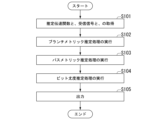
- 5 is a flowchart illustrating a first example of the flow of processing executed by the soft decision device in the embodiment.
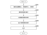
- 7 is a flowchart illustrating a second example of the flow of processing executed by the soft decision device in the embodiment.
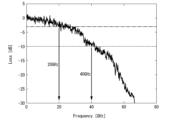
- the first diagram showing an example of experimental results in the embodiment.
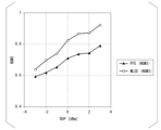
- the second diagram showing an example of experimental results in the embodiment.
- the figure which shows the example of a structure of the control part in embodiment. 7 is a flowchart illustrating a third example of the flow of processing executed by the soft decision device in the embodiment.
- FIG. 1 is an explanatory diagram illustrating an optical transmission system 100 according to an embodiment.
- the optical transmission system 100 includes a transmitter 1, a transmission path 2, a receiver 3, and a soft decision device 4.
- Transmitter 1 transmits an optical signal.
- the optical signal transmitted by the transmitter 1 will be referred to as a transmission signal.
- the symbol multilevel degree of the transmission signal was m (m is an integer of 1 or more).
- the symbol of the transmitted signal will be referred to as a main symbol.
- the transmission line 2 is a transmission line, such as an optical fiber, through which an optical signal propagates.
- the transmission signal transmitted by the transmitter 1 propagates through the transmission path 2 and reaches the receiver 3.
- the receiver 3 receives the optical signal propagated through the transmission path 2.
- the result of the receiver receiving the optical signal propagated through the transmission path 2 will be referred to as a received signal.
- H is a vector whose elements are weighting coefficients. Therefore, h 1 , . . . , h l are all weighting coefficients.
- l is the memory length. That is, l is the time spread of the transfer function.
- x n is a symbol string indicating a transmission signal, and is a symbol string having symbols from the (n-l+1)th symbol to the nth symbol.
- a dot ( ⁇ ) means an inner product.
- W n represents white noise added to the optical signal by propagating through the transmission path 2 .
- the soft decision device 4 performs a soft decision on the (n+1)th (n is an integer from 1 to N, where N is an integer from 1 to 1) symbol of the transmission signal.
- the soft decision device 4 includes a control unit 40 including a processor 91 such as a CPU (Central Processing Unit) and a memory 92 connected via a bus, and executes a program.
- a processor 91 such as a CPU (Central Processing Unit)
- a memory 92 connected via a bus
- FIG. 2 is an explanatory diagram illustrating the Viterbi algorithm in the embodiment. More specifically, FIG. 2 is a trellis diagram illustrating the Viterbi algorithm.
- R is the value obtained by subtracting 1 from m raised to the (l-1) power.
- the state of the transmission signal at time n is the symbol of the transmission signal at time n.
- the symbol at time n of the transmission signal means the n-th symbol in the transmission signal.
- the four states are expressed as S 0 , S 1 , S 2 , and S 3 .
- the state S0 is a symbol expressed by an ordered set of "0" bits and "0" bits.
- State S1 is a symbol expressed by an ordered set of "0" bits and "1” bits.
- State S2 is a symbol expressed by an ordered set of "1” bits and "0” bits.
- State S3 is a symbol expressed by an ordered set of "1" bits and "1” bits.
- the path metric p M n+1 (M is an integer greater than or equal to 0 and less than or equal to R) is a quantity called a path metric in the Viterbi algorithm. Therefore, the path metric p M n+1 is a distance obtained by the Viterbi algorithm, a distance indicated by a predetermined distance function, and a distance indicating the likelihood that the symbol at time (n+1) of the transmitted signal is S r . be.
- the path metric p M n+1 may be the sum of the distance indicating the likelihood that the symbol at time (n+1) of the transmitted signal is S r and the distance of the first to nth remaining paths of the transmitted signal.
- the distance of the predetermined distance function may be, for example, a squared error or a sum of squared errors.
- the distance indicated by the branch metric may be, for example, a squared error or the sum of squared errors.
- the distance of the predetermined distance function in the path metric may be different from the distance of the predetermined distance function in the branch metric. Therefore, for example, when the distance indicated by the branch metric is a squared error, the distance indicated by the path metric is the sum of squared errors.
- the distance indicated by the branch metric when it becomes state S 1 at time n is b 1 n .
- the value of the branch metric is calculated based on the estimated transfer function, which is a previously obtained estimation result of the transfer function of the transmission path 2, and the received signal.
- the estimated transfer function is estimated, for example, based on the result of propagating a training signal prepared in advance to the receiver 3 via the transmission path 2.
- the process of calculating the branch metric value based on the estimated transfer function and the received signal may be any existing process.
- the process of calculating the value of the branch metric based on the estimated transfer function and the received signal calculates the square error between the received signal and the result of applying the estimated transfer function to the symbol sequence indicated by the branch metric. This is the process of obtaining.
- the symbol sequence indicated by the branch metric means a candidate sequence corresponding to the branch corresponding to the branch metric.
- the (n+1)th path metric is the sum of the nth path metric of the transition source and the branch metric that indicates the likelihood of transition from the nth state of the transition source to the (n+1)th state of the transition destination. be.
- the control unit 40 performs, for example, a first soft decision process as a process for performing a soft decision on the (n+1)th (n is an integer from 1 to N, N is an integer from 1 to N) symbol of the transmission signal.
- the first soft decision process is a process that includes a branch metric estimation process, a path metric estimation process, and a bit likelihood estimation process.
- the branch metric estimation process is based on the estimated transfer function, which is a pre-obtained estimation result of the transfer function of the transmission path 2, and the received signal. This is a process of estimating the likelihood of transition from a symbol to each candidate for the (n+1)th symbol.
- the likelihood of transition from the n-th symbol of the transmission signal to each candidate for the (n+1)-th symbol is a quantity called a branch metric in the Viterbi algorithm. Therefore, states S 0 , S 1 , S 2 , and S 3 in the example of FIG. 2 are examples of candidates.
- the path metric estimation process estimates the likelihood that each candidate for the (n+1)th symbol of the transmitted signal is a symbol of the transmitted signal, which is the likelihood obtained by the Viterbi algorithm, based on the result of the branch metric estimation process. It is processing.
- the likelihood obtained by the Viterbi algorithm that each candidate for the (n+1)th symbol of the transmitted signal is a symbol of the transmitted signal is a quantity called the path metric in the Viterbi algorithm. It is.
- Bit likelihood estimation processing uses the path metric of each candidate for the (n+1)th symbol of the transmitted signal to estimate the kth bit (k is an integer between 1 and m) in the (n+1)th symbol of the transmitted signal. This is a process of estimating the likelihood that is a predetermined bit.
- the path metric of each candidate for the (n+1)th symbol of the transmission signal is a path metric obtained by path metric estimation processing.
- the bit likelihood estimation process is a process that does not use path metrics other than the path metric of each candidate for the (n+1)th symbol of the transmission signal.
- the control unit 40 obtains the likelihood estimated by the bit likelihood estimation process as a soft decision result for the (n+1)th symbol of the transmission signal.
- the likelihood estimated by the bit likelihood estimation process is expressed, for example, by the following equation (1).
- the left side ⁇ k,n of equation (1) is the likelihood estimated by bit likelihood estimation processing, and indicates the likelihood that the k-th bit of the n-th symbol of the transmission signal is 0. Note that in the example of equation (1), there are two types of bits: 0 and 1. Therefore, information indicating the likelihood that the bit is 0 is also information indicating the likelihood that the bit is 1.
- bit likelihood estimation process when the likelihood estimated by the bit likelihood estimation process is expressed by equation (1), the bit likelihood estimation process also includes information indicating the standard deviation of the distribution of noise added to the optical signal in the transmission path 2. used.
- the standard deviation of the distribution of noise added to the optical signal on the transmission path 2 is, for example, a predetermined value.
- Equation (3) ⁇ Second example of likelihood in first soft decision processing>
- the likelihood estimated by the bit likelihood estimation process may be expressed by the following equation (3), for example.
- equation (1) is an approximate equation of equation (3).
- the content of the approximation is an approximation in which symbols other than the maximum symbol likelihood are replaced with 0.
- the left side ⁇ k,n of equation (3) is the likelihood estimated by bit likelihood estimation processing, and indicates the likelihood that the k-th bit of the n-th symbol of the transmission signal is 0. Note that in the example of equation (3), there are two types of bits: 0 and 1. Therefore, information indicating the likelihood that the bit is 0 is also information indicating the likelihood that the bit is 1.
- Equation (4) includes the value of the standard deviation of the distribution of noise added to the optical signal in the transmission path 2. Therefore, when the likelihood estimated by the bit likelihood estimation process is expressed by equation (3), the bit likelihood estimation process also includes information indicating the standard deviation of the distribution of noise added to the optical signal in the transmission path 2. used.
- the control unit 40 may perform, for example, a second soft-decision process as the process of performing a soft-decision on the (n+1)th (n is an integer from 1 to N, N is an integer from 1 to N) symbol of the transmission signal.
- the second soft decision process includes a hard decision process, a likelihood estimation process, and a difference acquisition process.
- Hard decision processing is processing that performs hard decisions using the Viterbi algorithm based on the estimated transfer function and the received signal.
- the likelihood estimation process calculates the likelihood of each candidate for the (n+1)th symbol of the transmitted signal (hereinafter referred to as "symbol candidate") based on the results of the hard decision process, the estimated transfer function, and the received signal. This is the process of estimating the States S 0 , S 1 , S 2 , and S 3 in the example of FIG. 2 are examples of symbol candidates.
- the likelihood estimated by the likelihood estimation process is called estimated likelihood.
- the difference acquisition process calculates the estimated likelihood of a symbol candidate whose k-th bit (k is an integer between 1 and K) is a predetermined bit, and the estimated likelihood of a symbol candidate whose k-th bit (k is an integer between 1 and K) is a predetermined bit. This is a process of obtaining the difference between the estimated likelihood of a symbol candidate that does not exist (hereinafter referred to as "likelihood difference").
- the control unit 40 acquires the likelihood difference obtained in the difference acquisition process as a soft decision result for the (n+1)th symbol of the transmission signal.
- H with a hat ( ⁇ ) as an accent symbol represents an estimated transfer function.
- y n represents a received signal.
- C ′ M,n expressed in equation (6) represents an ordered set of the result of the hard decision processing and the symbol u M , which is one of the candidates for the n-th symbol of the transmission signal.
- the ordered set C ' M,n will be referred to as an object ordered set.
- x′ n represents the n-th symbol of the transmitted signal estimated by hard decision processing. Note that l is the storage length as described above.
- Equation (7) When the estimated likelihood is expressed by Equation (5), the difference in likelihood is expressed, for example, by Equation (7) below. Note that in the example of equation (7), there are two types of bits: 0 and 1. Therefore, information indicating the likelihood that the bit is 0 is also information indicating the likelihood that the bit is 1.
- Equation (7) includes the value of the standard deviation of the distribution of noise added to the optical signal in the transmission path 2. Therefore, when the likelihood difference estimated in the difference acquisition process is expressed by equation (7), the difference acquisition process also uses information indicating the standard deviation of the distribution of noise added to the optical signal in the transmission path 2.
- the estimated likelihood may be expressed by the following equation (8), for example.
- equation (5) is obtained by normalizing equation (8) and taking the natural logarithm.
- coefficients that do not depend on M and n are normalized.
- Equation (8) includes the value of the standard deviation of the distribution of noise added to the optical signal in the transmission path 2. Therefore, when the likelihood estimated in the likelihood estimation process is expressed by equation (8), the information indicating the standard deviation of the distribution of noise added to the optical signal in the transmission path 2 is also used in the likelihood estimation process. .
- Equation (9) the difference in likelihood is expressed, for example, by Equation (9) below. Note that in the example of equation (9), there are two types of bits: 0 and 1. Therefore, information indicating the likelihood that the bit is 0 is also information indicating the likelihood that the bit is 1.
- the estimated likelihood may be obtained, for example, based on the difference between the received signal and the result of applying the estimated transfer function to the result of hard decision processing.
- the difference between the result of applying the estimated transfer function to the result of the hard decision process and the received signal represents the result of estimating the noise distribution.
- the distribution of the difference between the result of applying the estimated transfer function to the result of hard decision processing and the received signal is the result of estimating the noise distribution, so W is a quantity representing the result of estimating the noise.
- the modified likelihood estimation process is a process of estimating the likelihood of each candidate for the (n+1)th symbol of the transmitted signal based on the result of the hard decision process, the estimated transfer function, and the received signal. This is a type of likelihood estimation process.
- the result of the hard decision process used in the modified likelihood estimation process is the result of the hard decision process for l symbols before the estimation target in the modified likelihood estimation process. Therefore, for example, when a candidate for the (n+1)th symbol of the transmission signal is an estimation target by the modified likelihood estimation process, hard decisions are performed on l symbols before the nth in the hard decision process.
- a histogram with a predetermined class width is generated for the noise W having the number of samples ⁇ .
- the horizontal axis of the histogram represents class, and the vertical axis represents frequency.
- the processing for noise with the number of samples ⁇ means the processing for a set whose element is noise W and whose number of elements is ⁇ .
- the number of samples in each class is then normalized by the number of samples in the class with the largest number of samples.
- the number of samples belonging to the class that includes the difference between the received signal and the result of applying the estimated transfer function to the target ordered set C ' M,n is calculated.
- the number of normalized samples is taken as the likelihood at each symbol. Note that the meaning of ⁇ includes the difference between the received signal and the result of applying the estimated transfer function to the target ordered set C'M ,n'' is specifically the likelihood of the symbol M at the time index n. means to select the class corresponding to .
- FIG. 3 is a diagram showing an example of the hardware configuration of the soft decision device 4 in the embodiment.
- the soft decision device 4 includes a control unit 40 including a processor 91 such as a CPU and a memory 92 connected via a bus, and executes a program.
- the soft decision device 4 functions as a device including a control section 40, an interface section 41, and a storage section 42 by executing a program.
- the processor 91 reads a program stored in the storage unit 42 and stores the read program in the memory 92.
- the soft decision device 4 functions as a device including the control section 40, the interface section 41, and the storage section 42.
- the control unit 40 controls the operations of various functional units included in the soft decision device 4.
- the control unit 40 executes, for example, a first soft decision process.
- the control unit 40 executes, for example, a second soft decision process instead of the first soft decision process.
- the interface unit 41 includes an interface for connecting the soft decision device 4 to an external device.
- the interface unit 41 communicates with an external device via wire or wireless.
- the external device is, for example, the receiver 3.
- the interface unit 41 acquires, for example, the received signal acquired by the receiver 3.
- the interface unit 41 includes input devices such as a mouse, a keyboard, and a touch panel.
- the interface unit 41 may include an interface that connects these input devices to the soft decision device 4.
- the interface unit 41 includes a display device such as a CRT (Cathode Ray Tube) display, a liquid crystal display, and an organic EL (Electro-Luminescence) display.
- the interface unit 41 may include an interface that connects these display devices to the soft decision device 4.
- the storage unit 42 is configured using a non-transitory computer-readable recording medium such as a magnetic hard disk device or a semiconductor storage device.
- the storage unit 42 stores various information regarding the soft decision device 4.
- the storage unit 42 may store various types of information generated as a result of processing executed by the control unit 40, for example.
- the storage unit 42 may store, for example, the received signal acquired by the interface unit 41.
- the storage unit 42 may store the estimated transfer function in advance, for example.
- FIG. 4 is a flowchart showing a first example of the flow of processing executed by the soft decision device 4 in the embodiment. More specifically, FIG. 4 is a flowchart illustrating an example of the flow of processing executed by the soft decision device 4 that executes the first soft decision processing.
- the control unit 40 acquires the estimated transfer function stored in the storage unit 42 and the received signal acquired by the interface unit 41 (step S101). Next, the control unit 40 executes branch metric estimation processing (step S102). Next, the control unit 40 executes path metric estimation processing (step S103).
- control unit 40 executes bit likelihood estimation processing (step S104).
- the control unit 40 obtains the likelihood estimated in the process of step S104 as a soft decision result for the (n+1)th symbol of the transmission signal.
- the control unit 40 controls the operation of the interface unit 41 to output the likelihood estimated in step S104 to the interface unit 41 (step S105).
- FIG. 5 is a flowchart showing a second example of the flow of processing executed by the soft decision device 4 in the embodiment. More specifically, FIG. 5 is a flowchart illustrating an example of the flow of processing executed by the soft decision device 4 that executes the second soft decision processing.
- the control unit 40 acquires the estimated transfer function stored in the storage unit 42 and the received signal acquired by the interface unit 41 (step S201). Next, the control unit 40 executes hard decision processing (step S202). Next, the control unit 40 executes likelihood estimation processing (step S203).
- control unit 40 executes a difference acquisition process (step S204).
- the control unit 40 obtains the likelihood difference obtained in the process of step S204 as a soft decision result for the (n+1)th symbol of the transmission signal.
- control unit 40 controls the operation of the interface unit 41 to output the likelihood difference estimated in step S204 to the interface unit 41 (step S205).
- the soft decision device 4 that executes the second soft decision process performs a soft decision on the main symbol, which is the (n+1)th symbol of the transmission signal with the symbol multilevel degree m.
- the soft decision device 4 that executes the second soft decision process includes a control unit 40.
- the control unit 40 performs hardening using the Viterbi algorithm based on an estimated transfer function that is a previously obtained estimation result of the transfer function of the transmission path 2 through which the transmitted signal propagates, and a received signal that is the result of receiving the transmitted signal. Execute hard decision processing to make a decision.
- the control unit 40 executes a likelihood estimation process for estimating the likelihood of each candidate for the (n+1)th symbol based on the result of the hard decision process, the estimated transfer function, and the received signal.
- the control unit 40 calculates the likelihood of a candidate whose k-th bit (k is an integer between 1 and m) is a predetermined bit, and the likelihood of a candidate whose k-th bit is not a predetermined bit. Execute the difference retrieval process to retrieve the difference between and. The control unit 40 outputs the obtained difference as a soft decision result.
- a comparison experiment was also conducted to evaluate the effectiveness of the experiment using the soft decision device 4.
- the technology used in the comparison experiment was a technology that did not use the soft decision device 4 (hereinafter referred to as "comparison technology"). More specifically, the technology to be compared is a technology that estimates a main symbol by applying an inverse function of a transfer function to a received signal.
- the transmitter 1 converted a digital signal indicating the content that the user wanted to transmit into an analog signal.
- the conversion in the experiment was 128 Gsample/s, 65 GHz conversion.
- the analog signal obtained by conversion was amplified by an amplifier.
- the transmitter 1 modulated a laser beam with a wavelength of 1310 nm using an amplified analog signal and outputted the result as an optical signal.
- the modulation method was PAM4.
- the optical signal output from the transmitter 1 entered the transmission line 2 and propagated through the transmission line 2.
- the transmission line 2 was a single mode fiber with a length of 10 km.
- the wavelength dispersion of the transmission line 2 was ⁇ 8 ps/nm at a wavelength of 1310 nm.
- the receiver 3 was equipped with a variable optical attenuator, and in the receiver 3, the power of the optical signal emitted from the transmission line 2 was attenuated by the variable optical attenuator.
- the receiver 3 used a photodiode to convert the optical signal whose power was attenuated by the variable optical attenuator into an electrical signal.
- the bandwidth of the photodiode was 50 GHz.
- the electrical signal obtained by the photodiode was amplified and then converted into a digital signal. Conversion to a digital signal was performed at 160 Gsample/s and 63 GHz.
- the converted signal is an example of a received signal, and was an example of a received signal in the experiment.
- the soft decision device 4 acquired the received signal obtained in this way.
- the control unit 40 included in the soft decision device 4 executed the first soft decision process, and acquired the likelihood estimated by the first soft decision process as the result of the soft decision. More specifically, in the experiment, the control unit 40 estimated the likelihood expressed by equation (1) by executing the first soft decision process.
- FIG. 6 is a first diagram showing an example of experimental results in the embodiment. More specifically, FIG. 6 is a diagram showing an example of experimental results using the comparative technology. The horizontal axis in FIG. 6 indicates frequency. The vertical axis in FIG. 6 indicates loss. FIG. 6 shows that when the comparative technology is used, the loss becomes large near a frequency of 60 GHz.
- FIG. 7 is a second diagram showing an example of experimental results in the embodiment.
- the horizontal axis in FIG. 7 indicates ROP (Received Optical Power).
- the vertical axis in FIG. 7 indicates normalized general mutual information (NGMI).
- NGMI Maximum Likelihood Sequence Estimation
- FFE(NGMI) Frimum Likelihood Sequence Estimation
- FIG. 7 means that the NGMI is higher when the first soft decision process is performed using the soft decision device 4 and the likelihood expressed by equation (1) is estimated than when using the comparative technology.
- FIG. 7 shows that by using the results of the soft decision made by the soft decision device 4, the main symbol can be estimated with higher accuracy than the comparative technology.
- the comparative technology estimates the main symbol by applying an inverse function of the transfer function to the received signal.
- the inverse function is applied, even the noise added to the signal in the transmission path 2 is amplified.
- the soft decision device 4 since the soft decision device 4 does not use the inverse function of the transfer function, noise will not be amplified. Therefore, the soft decision device 4 can estimate the main symbol with higher accuracy than the comparative technology.
- the soft decision device 4 configured in this way executes the first soft decision process or the second soft decision process. Therefore, since the soft decision result is obtained without using the inverse function of the transfer function, the soft decision device 4 can estimate the symbol of the transmission signal with higher accuracy.
- equations (1), (4), (7), and (8) include the standard deviation ⁇ of the distribution of noise imparted to the optical signal in the transmission path 2.
- the value of the standard deviation ⁇ of the distribution of noise added to the optical signal in the transmission path 2 may be a predetermined value, or may not be a predetermined value.
- the value of the standard deviation ⁇ may be obtained based on the difference between the received signal and the result of applying the estimated transfer function to the correct data.
- the correct answer data is data indicating the correct answer of the transmission signal. Therefore, for example, the standard deviation ⁇ may be obtained by the process expressed by the following equation (12).
- Equation (13) indicates the d-th symbol of the transmission signal indicated by the correct data.
- l in Equation (13) means the storage length of the estimated transfer function
- e in Equation (12) indicates the start position of the transmission signal indicated by the correct data.
- the start position indicates the position in the time axis direction in the correct data to be used.
- D represents the number of symbols used to calculate the standard deviation ⁇ .
- d means the time index in the correct answer data to be used. Therefore, Equation (12) represents the process of obtaining the average value of D estimated noises as the standard deviation ⁇ .
- Estimated noise is the square error between the received signal and the result of applying the estimated transfer function to the correct data.
- the value of standard deviation ⁇ may be obtained based on the difference between the received signal and the result of applying the estimated transfer function to the result of hard decision processing. Therefore, for example, the standard deviation ⁇ may be obtained by the process expressed by the following equation (14).
- Equation (15) indicates the d-th symbol of the transmission signal indicated by the result of the hard decision processing.
- l in Equation (15) means the storage length of the estimated transfer function
- e in Equation (14) indicates the start position of the transmission signal indicated by the result of hard decision processing.
- the start position indicates the position in the time axis direction in the hard decision processing result.
- D represents the number of symbols used to calculate the standard deviation ⁇ .
- d means the time index in the hard decision result to be used. Therefore, equation (14) represents the process of obtaining the average value of D estimated noises as the standard deviation ⁇ .
- the value of the standard deviation ⁇ may be a value that satisfies the condition of maximizing the NGMI.
- NGMI is, for example, a quantity defined by the following equation (16).
- the value of the soft output (that is, the result of the soft decision) may diverge to the plus or minus side.
- Some programming languages do not produce a value when they diverge. Therefore, in order to avoid a situation where no value is obtained, in the process of performing a soft decision on the (n+1)th symbol of the transmission signal, an upper or lower limit of the soft output value may be determined in advance.
- the soft decision device 4 may be implemented using a plurality of information processing devices that are communicably connected via a network.
- each functional unit included in the soft decision device 4 may be distributed and implemented in a plurality of information processing devices.
- the soft decision device 4 may be realized using hardware such as an ASIC (Application Specific Integrated Circuit), a PLD (Programmable Logic Device), or an FPGA (Field Programmable Gate Array). .
- the program may be recorded on a computer-readable recording medium.
- the computer-readable recording medium is, for example, a portable medium such as a flexible disk, magneto-optical disk, ROM, or CD-ROM, or a storage device such as a hard disk built into a computer system.
- the program may be transmitted via a telecommunications line.
- FIG. 8 is a diagram showing an example of the configuration of the control unit 40 in the embodiment.
- the control unit 40 includes a transfer function estimation unit 401, a branch metric processing unit 402, a path metric processing unit 403, a hard decision output unit 404, and a soft decision output unit 405.
- the transfer function estimation unit 401 calculates the estimated transfer function " ⁇ H" as shown in equation (19).
- the branch metric processing unit 402 calculates the branch metric "b" as shown in equation (20).
- the path metric processing unit 403 calculates the path metric "p" as shown in equation (21).
- the hard decision output unit 404 compares the path metric "p" of each state “s” for each time index.
- the hard decision output unit 404 selects the minimum path metric from among the path metrics of the " ml " states “s” at the time index "n” based on the comparison result of the path metrics "p".
- the path in the time direction made up of the branches used to calculate the selected minimum path metric is called a "survival path.”
- the hard decision output unit 404 generates a hard decision result "x' na " by backward calculation in the trellis diagram.
- the symbol determination result is expressed as in equation (22).
- a represents the number of times the path is traced in the direction opposite to the state transition direction (number of traces).
- s j represents the state at the trace destination “j”.
- the hard decision output unit 404 generates a hard decision result “x'' na ” by forward calculation in the trellis diagram. If the state with the minimum path metric at time index “n” is “s j ”, the symbol “x'' n ” determined as a result of the forward operation (path metric calculation and remaining path selection) is expressed by the formula ( 23). Note that the time index of state S j in equation (23) is different from the time index of state S j in equation (22). Therefore, it should be noted that the left side of equation (23) and the left side of equation (22) are not in an equal relationship.
- This determined symbol “x'' n ” is a determination obtained by using only forward calculations (path metric calculation and remaining path selection) without using backward calculations (tracing back the remaining paths). This is the result.
- the effect of sequence estimation of the sequence length including the number of backward calculations by backward calculation cannot be obtained.
- the symbol determination result “x' na” by backward calculation may be different from the symbol determination result "x' ' na " by forward calculation. be.
- the symbol determination result “x′ na ” by backward calculation is more likely to be accurate than the symbol determination result “x′ na ” by forward calculation.
- the log likelihood ratio " ⁇ M,n” is calculated based on path metric information obtained by forward calculation. Therefore, if the symbol determination result "x' na " of the backward operation is different from the symbol determination result "x'' na " of the forward operation, the logarithm estimated based on the path metric information of the forward operation The accuracy of the likelihood ratio " ⁇ " may not be high.
- the soft decision output unit 405 approximately incorporates the effect of path retracing (backward calculation) in the trellis diagram through simple calculation. That is, the soft decision output unit 405 replaces the soft decision result of a complicated backward computation with the soft decision result of a simple computation.
- the complexity of this simple calculation is, for example, comparable to the complexity of the Viterbi algorithm used in hard-decision maximum likelihood sequence estimation (MLSE).
- Equation (24) The log likelihood ratio “ ⁇ ′ k,n ” is expressed as in Equation (24) using Equation (25).
- Equation (24) The calculation of equation (24) is essentially the same as equation (7).
- n represents a time index (1 ⁇ n ⁇ N).
- k represents the number (1 ⁇ k ⁇ m) of the bit in the symbol determination result at the time index “n”.
- c′ k,n represents the k-th bit (0 or 1) of the symbol determination result “x′ n ” at the time index “n”.
- c′′ k,n represents the k-th bit (0 or 1) of the symbol determination result “x′′ n ” at the time index “n”.
- the soft decision output unit 405 acquires a predetermined positive constant “A” from the memory 92, for example.
- This constant "A” is predetermined, for example, so that the standard generalized mutual information (NGMI) is maximized according to the result of changing the positive variable at predetermined intervals. For example, by changing a variable that takes a value from 0.001 to 1.000 at intervals of 0.001, a log likelihood ratio " ⁇ " is calculated for each value of the variable.
- the value of the variable when the standard generalized mutual information is maximized is predetermined as a positive constant "A".
- the soft decision output unit 405 compares the symbol determination result “x ′ na ” of the backward operation and the symbol determination result “x′′ na ” of the forward operation bit by bit. If the symbol determination result “x ′ na ” and the symbol determination result “x′′ na ” are the same, the soft decision output unit 405 outputs the soft decision result “ ⁇ k, The log - likelihood ratio ⁇ ' k,na '' is output as ⁇ na' '.
- the soft decision output unit 405 uses the sign function “sgn” to calculate the equation (24). Obtain the sign of the log likelihood ratio “ ⁇ ' k,n ".
- the soft decision output unit 405 obtains the sign of the log-likelihood ratio “ ⁇ k,n ” of Equation (1) instead of obtaining the sign of the log-likelihood ratio “ ⁇ k,n ” of Equation (24). You may.
- the soft decision output unit 405 determines the difference based on the sign opposite to the sign of the log-likelihood ratio “ ⁇ ' k,n ”, a predetermined constant “A”, and the standard deviation “ ⁇ ” of the noise distribution. , calculates a new soft decision result “ ⁇ k,na ”.
- the soft decision result “ ⁇ k, na ” (log-likelihood ratio) in the case where the symbol decision result “x′ na ” and the symbol decision result “x'' na ” are the same, and the symbol decision result “ x' na ' ' and the new soft decision result ⁇ k, na ' ' (changed log-likelihood ratio) in the case where the symbol decision result ⁇ x'' na' ' is different. is expressed as in equation (26).
- FIG. 9 is a flowchart showing a third example of the flow of processing executed by the soft decision device 4 in the embodiment.
- the control unit 40 acquires the estimated transfer function stored in the storage unit 42 and the received signal acquired by the interface unit 41 (step S301). Next, the control unit 40 executes branch metric estimation processing (step S302). Next, the control unit 40 executes path metric estimation processing (step S303).
- the control unit 40 generates a symbol determination result of backward calculation and a symbol determination result of forward calculation by executing hard decision processing (step S304).
- the control unit 40 executes bit likelihood estimation processing based on the symbol determination result of the backward calculation, the symbol determination result of the forward calculation, and a predetermined constant "A" (step S305).
- the control unit 40 obtains the likelihood estimated in the process of step S305 as a result of the soft decision.
- the control unit 40 controls the operation of the interface unit 41 and causes the interface unit 41 to output the likelihood “ ⁇ k,na ” estimated in step S305 (step S306).
- the predetermined constant "A” is determined as “2 ⁇ 2 P" based on the likelihood "P” indicating a positive peak of the distribution and the standard deviation " ⁇ ".
- FIG. 10 is a diagram showing an example of a bit likelihood histogram in the embodiment.
- the soft decision output unit 405 acquires a predetermined positive constant “A” from the memory 92, for example. As illustrated in equation (26), the absolute value of the soft decision result is expressed as "A/2 ⁇ 2 ".
- FIG. 11 is a third diagram showing an example of experimental results in the embodiment.
- the symbol multilevel degree "M” is 4 as an example.
- the storage length "d” is 5 as an example.
- the number of traces "T” is 20, for example.
- the predetermined positive constant "A" in the second embodiment is, for example, 0.018.
- the number of path metrics "M d " required to calculate the log-likelihood ratio " ⁇ " in the first embodiment is 1024, for example.
- the number of path metrics “2M d ” required to calculate the log-likelihood ratio “ ⁇ ” in the second embodiment is 1024, as an example.
- the number of path metrics "M d+1 T" required to calculate the log-likelihood ratio " ⁇ " in the FFE method is, for example, 81920.
- the left graph in FIG. 11 shows the received optical intensity (ROP) and standard generalized mutual information (NGMI).
- Both the received light intensity of the NL-MLSE method in the first embodiment and the received light intensity of the NL-MLSE method in the second embodiment achieve higher standard generalized mutual information than the FFE method.
- the standard generalized mutual information is improved by about 18% in the first embodiment. Further, in the second embodiment, the standard generalized mutual information is improved by about 22%.
- the right graph in FIG. 11 shows the bit error rate (BER) and standard generalization for the FFE method, the NL-MLSE method in the first embodiment, and the NL-MLSE method in the second embodiment.
- the relationship with mutual information (NGMI) is shown.
- the dashed line overlapping the results of the FFE scheme represents the theoretical curve of the additive white Gaussian noise (AWGN) channel.
- the performance represented by the theoretical curve corresponds to the performance of the Soft Output Viterbi Algorithm (SOVA), which requires a very large amount of calculations, when the same BER as the NL-MLSE method is obtained.
- SOVA Soft Output Viterbi Algorithm
- the FFE method cannot achieve a code error rate of "0.8".
- the NL-MLSE method in the first embodiment can achieve a code error rate of "0.931”.
- the NL-MLSE method in the second embodiment can achieve a code error rate of "0.962". In this way, the optical transmission system 100 in the second embodiment can achieve performance close to the standard generalized mutual information "0.985" by the soft output Viterbi algorithm with a smaller amount of calculations.
- Optical transmission system 1... Transmitter, 2... Transmission path, 3... Receiver, 4... Soft decision device, 40... Control unit, 41... Interface unit, 42... Storage unit, 91... Processor, 92... Memory, 401...Transfer function estimation unit, 402...Branch metric processing unit, 403...Path metric processing unit, 404...Hard decision output unit, 405...Soft decision output unit
Landscapes
- Engineering & Computer Science (AREA)
- Physics & Mathematics (AREA)
- Probability & Statistics with Applications (AREA)
- Quality & Reliability (AREA)
- Electromagnetism (AREA)
- Computer Networks & Wireless Communication (AREA)
- Signal Processing (AREA)
- Theoretical Computer Science (AREA)
- Error Detection And Correction (AREA)
Abstract
シンボル多値度がmの送信信号、の(n+1)番目のシンボルに対する軟判定を行う軟判定装置であって、伝送路の伝達関数の推定結果である推定伝達関数と、受信信号と、に基づき、ビタビ・アルゴリズムで得られる距離であり距離関数における距離であり送信信号のn番目のシンボルから(n+1)番目のシンボルの各候補に遷移する尤度を示す距離であるブランチメトリックを推定し、前記ブランチメトリック推定処理の結果に基づき、ビタビ・アルゴリズムで得られる距離であり距離関数における距離であり送信信号の(n+1)番目のシンボルの各候補が送信信号のシンボルである尤度を示す距離と送信信号の所定の残存パスの距離との合計であるパスメトリックを推定し、送信信号の(n+1)番目のシンボルの各候補のパスメトリックを用い、送信信号の(n+1)番目のシンボルにおけるk番目のビットが所定のビットである尤度を推定する制御部、を備える軟判定装置。
Description
本発明は、軟判定装置、軟判定方法及びプログラムに関する。
本願は、2022年8月9日に国際出願されたPCT/JP2022/030392号に基づき優先権を主張し、その内容をここに援用する。
本願は、2022年8月9日に国際出願されたPCT/JP2022/030392号に基づき優先権を主張し、その内容をここに援用する。
近年のネットワークトラフィックの増大に対応するため、光伝送システムの高速化及び長距離化の検討が進められている。
D. D. Falconer, et al., ‘Adaptive channel memory truncation for maximum likelihood sequence estimation,’ The Bell System Technical Journal, vol. 52, no. 9, pp. 1541 - 1562 (1973)
しかしながら、光伝送システムでは高速化及び長距離化に伴い信号の歪や雑音が増大する。そのため、送信機によって送信された光信号である送信信号のシンボルを推定する技術が必要とされており、伝送路の伝達関数の逆関数を用いて送信信号のシンボルを推定することが提案されている。しかしながら、提案された技術を用いた推定は精度が低い場合があった。
上記事情に鑑み、本発明は、送信信号のシンボルをより高精度に推定する技術を提供することを目的としている。
本発明の一態様は、シンボル多値度がm(mは2以上の整数)の送信信号、の(n+1)番目(nは1以上N以下の整数。Nは1以上の整数)のシンボルである主シンボルに対する軟判定を行う軟判定装置であって、前記送信信号が伝搬する伝送路の伝達関数の予め得られた推定結果である推定伝達関数と、前記送信信号の受信の結果である受信信号と、に基づき、ビタビ・アルゴリズムで得られる距離であり所定の距離関数が示す距離であり前記送信信号のn番目のシンボルから(n+1)番目のシンボルの各候補に遷移する尤度を示す距離であるブランチメトリックを推定するブランチメトリック推定処理と、前記ブランチメトリック推定処理の結果に基づき、ビタビ・アルゴリズムで得られる距離であり所定の距離関数が示す距離であり前記送信信号の(n+1)番目のシンボルの各候補が前記送信信号のシンボルである尤度を示す距離と、前記送信信号の1番目からn番目の残存パスの距離との合計であるパスメトリックを推定するパスメトリック推定処理と、前記パスメトリック推定処理によって得られた前記送信信号の(n+1)番目のシンボルの各候補のパスメトリックを用い、前記送信信号の(n+1)番目のシンボルの各候補のパスメトリック以外のパスメトリックは用いずに、前記送信信号の(n+1)番目のシンボルにおけるk番目(kは1以上m以下の整数)のビットが所定のビットである尤度を推定するビット尤度推定処理と、を実行する制御部、を備え、前記制御部は、前記ビット尤度推定処理で推定された尤度を、前記軟判定の結果として取得する、軟判定装置である。
本発明の一態様は、シンボル多値度がm(mは2以上の整数)の送信信号、の(n+1)番目(nは1以上N以下の整数。Nは1以上の整数)のシンボルである主シンボルに対する軟判定を行う軟判定方法であって、前記送信信号が伝搬する伝送路の伝達関数の予め得られた推定結果である推定伝達関数と、前記送信信号の受信の結果である受信信号と、に基づき、ビタビ・アルゴリズムで得られる距離であり所定の距離関数が示す距離であり前記送信信号のn番目のシンボルから(n+1)番目のシンボルの各候補に遷移する尤度を示す距離であるブランチメトリックを推定するブランチメトリック推定処理と、前記ブランチメトリック推定処理の結果に基づき、ビタビ・アルゴリズムで得られる距離であり所定の距離関数が示す距離であり前記送信信号の(n+1)番目のシンボルの各候補が前記送信信号のシンボルである尤度を示す距離と、前記送信信号の1番目からn番目の残存パスの距離との合計であるパスメトリックを推定するパスメトリック推定処理と、前記パスメトリック推定処理によって得られた前記送信信号の(n+1)番目のシンボルの各候補のパスメトリックを用い、前記送信信号の(n+1)番目のシンボルの各候補のパスメトリック以外のパスメトリックは用いずに、前記送信信号の(n+1)番目のシンボルにおけるk番目(kは1以上m以下の整数)のビットが所定のビットである尤度を推定するビット尤度推定処理と、を実行する制御ステップ、を有し、前記制御ステップは、前記ビット尤度推定処理で推定された尤度を、前記軟判定の結果として取得する、軟判定方法である。
本発明の一態様は、上記の軟判定装置としてコンピュータを機能させるためのプログラムである。
本発明により、送信信号のシンボルをより高精度に推定することが可能となる。
(第1実施形態)
図1は、実施形態の光伝送システム100を説明する説明図である。光伝送システム100は、送信機1、伝送路2、受信機3及び軟判定装置4を備える。送信機1は、光信号を送信する。以下、送信機1の送信する光信号を送信信号という。光伝送システム100において、送信信号のシンボル多値度はm(mは1以上の整数)であった。以下、送信信号のシンボルを主シンボルという。
図1は、実施形態の光伝送システム100を説明する説明図である。光伝送システム100は、送信機1、伝送路2、受信機3及び軟判定装置4を備える。送信機1は、光信号を送信する。以下、送信機1の送信する光信号を送信信号という。光伝送システム100において、送信信号のシンボル多値度はm(mは1以上の整数)であった。以下、送信信号のシンボルを主シンボルという。
伝送路2は、光ファイバ等の、光信号が伝搬する伝送路である。送信機1の送信した送信信号は伝送路2を伝搬し受信機3に到達する。受信機3は、伝送路2を伝搬してきた光信号を受信する。以下、伝送路2を伝搬してきた光信号を受信機が受信した結果を受信信号という。
伝送路2の伝達関数をベクトルH={h1、・・・、hl}と表すと、受信信号ynは、xn・H+Wnである。Hは重み係数を要素とするベクトルである。したがって、h1、・・・、hlはいずれも、重み係数である。lは記憶長である。すなわち、lは伝達関数の時間広がりである。xnは送信信号を示すシンボル列であり、(n-l+1)番目のシンボルからn番目のシンボルからまでのシンボルを有するシンボル列である。ドット(・)は内積を意味する。Wnは、伝送路2を伝搬することで光信号に付与される白色雑音を表す。
軟判定装置4は、送信信号の(n+1)番目(nは1以上N以下の整数。Nは1以上の整数)のシンボルに対する軟判定を行う。軟判定装置4は、バスで接続されたCPU(Central Processing Unit)等のプロセッサ91とメモリ92とを備える制御部40を備え、プログラムを実行する。
<ビタビ・アルゴリズム>
軟判定装置4による軟判定では、ビタビ・アルゴリズムにおいて定義される量が用いられる。そこで軟判定装置4による軟判定の説明に先立ち、念のため、ビタビ・アルゴリズムについて説明する。説明の簡単のため、記憶長l=3、シンボル多値度m=2の場合を例に説明を行う。また、信号が0と1との2つのビットの系列である場合を例に説明を行う。
軟判定装置4による軟判定では、ビタビ・アルゴリズムにおいて定義される量が用いられる。そこで軟判定装置4による軟判定の説明に先立ち、念のため、ビタビ・アルゴリズムについて説明する。説明の簡単のため、記憶長l=3、シンボル多値度m=2の場合を例に説明を行う。また、信号が0と1との2つのビットの系列である場合を例に説明を行う。
図2は、実施形態におけるビタビ・アルゴリズムを説明する説明図である。より具体的には図2は、ビタビ・アルゴリズムを説明するトレリス図である。
シンボル多値度m=2であり記憶長l=3であるため、送信信号の各時刻nにおける状態の候補は、(R+1)通りである。Rは、mの(l-1)乗から1を引き算した値である。図2において、送信信号の時刻nにおける状態の候補は4通りであり、R=3である。送信信号の時刻nにおける状態とは、具体的には、送信信号の時刻nのシンボルである。なお、送信信号の時刻nのシンボルとは、送信信号におけるn番目のシンボルの意味である。図2において4通りの各状態は、S0、S1、S2、S3と表現されている。
状態S0は「0」ビットと「0」ビットとの順序集合で表現されるシンボルである。状態S1は「0」ビットと「1」ビットとの順序集合で表現されるシンボルである。状態S2は「1」ビットと「0」ビットとの順序集合で表現されるシンボルである。状態S3は「1」ビットと「1」ビットとの順序集合で表現されるシンボルである。
pM
n+1は(Mは0以上R以下の整数である)、ビタビ・アルゴリズムにおいてパスメトリックと呼称される量である。したがって、パスメトリックpM
n+1は、ビタビ・アルゴリズムで得られる距離であり、所定の距離関数が示す距離であり、送信信号の時刻(n+1)におけるシンボルがSrである尤度を示す距離、である。パスメトリックpM
n+1は、送信信号の時刻(n+1)におけるシンボルがSrである尤度を示す距離と、送信信号の1番目からn番目の残存パスの距離との合計でもよい。なお、所定の距離関数の距離は、例えば二乗誤差であってもよいし、二乗誤差の総和であってもよい。
bq
n+1は(qは1以上Q以下の整数である。Q=(R+1)×mである。)、ビタビ・アルゴリズムにおいてブランチメトリックと呼称される量である。したがって、ブランチメトリックbq
n+1は、ビタビ・アルゴリズムで得られる距離であり、所定の距離関数が示す距離であり、送信信号のn番目のシンボルから(n+1)番目のシンボルの各候補に遷移する尤度を示す距離である。シンボル多値度がm=2であるので、(n+1)番目のシンボルは、n番目のシンボルの各候補に続く次のビットは0又は1のいずれかである。したがってブランチメトリックの数Qは、(R+1)×mである。
ブランチメトリックが示す距離は、例えば二乗誤差であってもよいし、二乗誤差の総和であってもよい。パスメトリックにおける所定の距離関数の距離と、ブランチメトリックにおける所定の距離関数の距離とは異なってもよい。したがって例えば、ブランチメトリックの示す距離が二乗誤差である場合に、パスメトリックの示す距離は二乗誤差の総和である。
図2の例では、例えば時刻(n-1)のシンボルが状態S0である場合、時刻nにおいて状態S1となる場合のブランチメトリックの示す距離がb1
nである。
ブランチメトリックの値は、伝送路2の伝達関数の予め得られた推定結果である推定伝達関数と、受信信号と、に基づき算出される。推定伝達関数は、例えば、予め用意されたトレーニング信号を、伝送路2を介して受信機3まで伝搬させた結果に基づいて推定される。
推定伝達関数と、受信信号と、に基づくブランチメトリックの値の算出の処理は、既存のどのような処理であってもよい。推定伝達関数と、受信信号と、に基づくブランチメトリックの値の算出の処理は、例えば、受信信号と、ブランチメトリックが示すシンボル系列に対して推定伝達関数を作用させた結果と、の二乗誤差を得る処理である。なお、ブランチメトリックが示すシンボル系列とは、ブランチメトリックに対応するブランチ、に対応する候補系列を意味する。
(n+1)番目のパスメトリックは、遷移元のn番目のパスメトリックと、遷移元のn番目の状態から遷移先の(n+1)番目の状態への遷移の尤度を示すブランチメトリックとの和である。
ビタビ・アルゴリズムは、このようにしてパスメトリックとブランチメトリックとを時刻n=1からn=Nまで逐次的に算出する処理である。
<第1軟判定処理>
図1の説明に戻る。制御部40は、送信信号の(n+1)番目(nは1以上N以下の整数。Nは1以上の整数)のシンボルに対する軟判定を行う処理として、例えば第1軟判定処理を行う。第1軟判定処理は、ブランチメトリック推定処理と、パスメトリック推定処理と、ビット尤度推定処理と、を含む処理である。
図1の説明に戻る。制御部40は、送信信号の(n+1)番目(nは1以上N以下の整数。Nは1以上の整数)のシンボルに対する軟判定を行う処理として、例えば第1軟判定処理を行う。第1軟判定処理は、ブランチメトリック推定処理と、パスメトリック推定処理と、ビット尤度推定処理と、を含む処理である。
ブランチメトリック推定処理は、伝送路2の伝達関数の予め得られた推定結果である推定伝達関数と、受信信号と、に基づき、ビタビ・アルゴリズムで得られる尤度であって送信信号のn番目のシンボルから(n+1)番目のシンボルの各候補に遷移する尤度を推定する処理である。上述したように、送信信号のn番目のシンボルから(n+1)番目のシンボルの各候補に遷移する尤度は、ビタビ・アルゴリズムにおいてブランチメトリックと呼称される量である。したがって図2の例における状態S0、S1、S2、S3は、候補の一例である。
パスメトリック推定処理は、ブランチメトリック推定処理の結果に基づき、ビタビ・アルゴリズムで得られる尤度であって送信信号の(n+1)番目のシンボルの各候補が送信信号のシンボルである尤度を推定する処理である。上述したように、ビタビ・アルゴリズムで得られる尤度であって送信信号の(n+1)番目のシンボルの各候補が送信信号のシンボルである尤度は、ビタビ・アルゴリズムにおいてパスメトリックと呼称される量である。
ビット尤度推定処理は、送信信号の(n+1)番目のシンボルの各候補のパスメトリックを用いて、送信信号の(n+1)番目のシンボルにおけるk番目(kは1以上m以下の整数)のビットが所定のビットである尤度を推定する処理、である。送信信号の(n+1)番目のシンボルの各候補のパスメトリックは、パスメトリック推定処理によって得られたパスメトリックである。ビット尤度推定処理は、送信信号の(n+1)番目のシンボルの各候補のパスメトリック以外のパスメトリックは用いない処理である。
制御部40は、ビット尤度推定処理で推定された尤度を、送信信号の(n+1)番目のシンボルに対する軟判定の結果として取得する。
<第1軟判定処理における尤度の第1の例>
ビット尤度推定処理で推定される尤度は、例えば以下の式(1)で表される。式(1)の左辺λk、nがビット尤度推定処理で推定される尤度であり、送信信号のn番目のシンボルのk番目のビットが0である尤度を示す。なお、式(1)の例ではビットが0と1との2種類である。したがって、ビットが0である尤度を示す情報は、ビットが1である尤度を示す情報でもある。
ビット尤度推定処理で推定される尤度は、例えば以下の式(1)で表される。式(1)の左辺λk、nがビット尤度推定処理で推定される尤度であり、送信信号のn番目のシンボルのk番目のビットが0である尤度を示す。なお、式(1)の例ではビットが0と1との2種類である。したがって、ビットが0である尤度を示す情報は、ビットが1である尤度を示す情報でもある。


ck、nは、送信信号のn番目のシンボルのk番目のビットを表す。σは、伝送路2で光信号に付与される雑音の分布の標準偏差を表す。したがって、ビット尤度推定処理で推定される尤度が式(1)で表される場合、ビット尤度推定処理では伝送路2で光信号に付与される雑音の分布の標準偏差を示す情報も用いられる。
伝送路2で光信号に付与される雑音の分布の標準偏差は、例えば予め定められた値である。なおuMはシンボル値の候補を表す。すなわちuMはu0~uRの各シンボル値を表す。したがって、例えば変調方式がPAM4の場合、例えばuMは、M=0であればu0=[c1,n、c2,n]=[0、0]を表し、M=1であればu1=[c1,n、c2,n]=[0、1]を表し、M=2であればu2=[c1,n、c2,n]=[1、1]を表し、M=3であればu3=[c1,n、c2,n]=[1、0]を表す。
<第1軟判定処理における尤度の第2の例>
ビット尤度推定処理で推定される尤度は、例えば以下の式(3)で表されてもよい。なお、式(1)は式(3)の近似式である。近似の内容は、具体的には、最大のシンボル尤度以外を0へと置き換える近似である。
ビット尤度推定処理で推定される尤度は、例えば以下の式(3)で表されてもよい。なお、式(1)は式(3)の近似式である。近似の内容は、具体的には、最大のシンボル尤度以外を0へと置き換える近似である。
式(3)の左辺λk、nがビット尤度推定処理で推定される尤度であり、送信信号のn番目のシンボルのk番目のビットが0である尤度を示す。なお、式(3)の例ではビットが0と1との2種類である。したがってビットが0である尤度を示す情報は、ビットが1である尤度を示す情報でもある。


式(4)には伝送路2で光信号に付与される雑音の分布の標準偏差の値が含まれている。したがって、ビット尤度推定処理で推定される尤度が式(3)で表される場合、ビット尤度推定処理では伝送路2で光信号に付与される雑音の分布の標準偏差を示す情報も用いられる。
<第2軟判定処理>
制御部40は、送信信号の(n+1)番目(nは1以上N以下の整数。Nは1以上の整数)のシンボルに対する軟判定を行う処理として、例えば第2軟判定処理を行ってもよい。第2軟判定処理は、硬判定処理と、尤度推定処理と、違い取得処理とを含む。
制御部40は、送信信号の(n+1)番目(nは1以上N以下の整数。Nは1以上の整数)のシンボルに対する軟判定を行う処理として、例えば第2軟判定処理を行ってもよい。第2軟判定処理は、硬判定処理と、尤度推定処理と、違い取得処理とを含む。
硬判定処理は、推定伝達関数と受信信号とに基づき、ビタビ・アルゴリズムによる硬判定を行う処理である。
尤度推定処理は、送信信号の(n+1)番目のシンボルの候補(以下「シンボル候補」という。)ごとに、硬判定処理の結果と推定伝達関数と受信信号とに基づいて各候補の尤度を推定する処理である。図2の例における状態S0、S1、S2、S3はシンボル候補の一例である。尤度推定処理で推定された尤度を推定尤度という。
違い取得処理は、シンボル候補のうちk番目(kは1以上K以下の整数)のビットが所定のビットであるシンボル候補の推定尤度と、シンボル候補のうちk番目のビットが所定のビットでは無いシンボル候補の推定尤度と、の違い(以下「尤度違い」という。)を取得する処理である。
制御部40は、違い取得処理で得られた尤度違いを、送信信号の(n+1)番目のシンボルに対する軟判定の結果として取得する。
<第2軟判定処理における推定尤度の第1の例>
推定尤度は、例えば以下の式(5)で表される。
推定尤度は、例えば以下の式(5)で表される。


式(5)にある、ハット(^)がアクセント記号として付いたHは、推定伝達関数を表す。ynは、受信信号を表す。式(6)で表されるC´M、nは、硬判定処理の結果と、送信信号のn番目のシンボルの候補のひとつであるシンボルuMと、の順序集合を表す。以下、順序集合C´M、nを対象順序集合という。x´nは、硬判定処理で推定された送信信号のn番目のシンボルを表す。なおlは上述したように記憶長である。
推定尤度が式(5)で表される場合、尤度違いは、例えば以下の式(7)で表される。なお、式(7)の例ではビットが0と1との2種類である。したがって、ビットが0である尤度を示す情報は、ビットが1である尤度を示す情報でもある。

式(7)には伝送路2で光信号に付与される雑音の分布の標準偏差の値が含まれる。したがって、違い取得処理で推定される尤度違いが式(7)で表される場合、違い取得処理では伝送路2で光信号に付与される雑音の分布の標準偏差を示す情報も用いられる。
<第2軟判定処理における推定尤度の第2の例>
推定尤度は、例えば以下の式(8)で表されてもよい。なお、式(5)は式(8)を規格化し、自然対数を取ったものである。ここでM及びnに依存しない係数を規格化している。
推定尤度は、例えば以下の式(8)で表されてもよい。なお、式(5)は式(8)を規格化し、自然対数を取ったものである。ここでM及びnに依存しない係数を規格化している。

式(8)には伝送路2で光信号に付与される雑音の分布の標準偏差の値が含まれる。したがって、尤度推定処理で推定される尤度が式(8)で表される場合、尤度推定処理では伝送路2で光信号に付与される雑音の分布の標準偏差を示す情報も用いられる。
推定尤度が式(8)で表される場合、尤度違いは、例えば以下の式(9)で表される。なお、式(9)の例ではビットが0と1との2種類である。したがって、ビットが0である尤度を示す情報は、ビットが1である尤度を示す情報でもある。

<第2軟判定処理における推定尤度の第3の例>
推定尤度は、例えば、推定伝達関数を硬判定処理の結果に作用させた結果と受信信号との違いに基づいて得られてもよい。推定伝達関数を硬判定処理の結果に作用させた結果と受信信号との違いは、雑音分布の推定結果を表す。
推定尤度は、例えば、推定伝達関数を硬判定処理の結果に作用させた結果と受信信号との違いに基づいて得られてもよい。推定伝達関数を硬判定処理の結果に作用させた結果と受信信号との違いは、雑音分布の推定結果を表す。
推定伝達関数を硬判定処理の結果に作用させた結果と受信信号との違いは、具体的には、以下の式(10)で表される。

式(10)において太字で表されたx´nは以下の式(11)の順序集合を意味する。

上述したように推定伝達関数を硬判定処理の結果に作用させた結果と受信信号との違いの分布は、雑音分布の推定結果であるので、Wは雑音の推定結果を表す量である。
以下、推定伝達関数を硬判定処理の結果に作用させた結果と受信信号との違いの分布に基づいて送信信号の(n+1)番目のシンボルの候補の推定尤度を得る処理を、変形尤度推定処理という。変形尤度推定処理は、送信信号の(n+1)番目のシンボルの候補ごとに、硬判定処理の結果と推定伝達関数と受信信号とに基づいて各候補の尤度を推定する処理であるので、尤度推定処理の1種である。
なお式(11)からわかるように、変形尤度推定処理において用いられる硬判定処理の結果は、変形尤度推定処理における推定対象より前のl個のシンボルに対する硬判定処理の結果である。したがって例えば、送信信号の(n+1)番目のシンボルの候補が変形尤度推定処理による推定対象である場合、硬判定処理では、n番目以前のl個のシンボルに対する硬判定が行われる。
変形尤度推定処理では、例えば、サンプル数αの雑音Wに対して所定の階級幅のヒストグラムを生成することが行われる。ヒストグラムの横軸は階級を表し、縦軸は度数を表す。なお、サンプル数αの雑音に対する処理は、要素が雑音Wであり要素数がαの集合に対する処理を意味する。このような場合、変形尤度推定処理では次に、各階級におけるサンプル数が最大のサンプル数を持つ階級のサンプル数で規格化される。
このような場合、変形尤度推定処理では次に、対象順序集合C´M、nに対して推定伝達関数を作用させた結果と受信信号との違いが含まれる階級、に属するサンプルの数であって規格化されたサンプルの数が、各シンボルにおける尤度として取得される。なお、対象順序集合C´M、nに対して推定伝達関数を作用させた結果と受信信号との違いが含まれる、との意味は、具体的には、時間インデックスnにおけるシンボルMの尤度に対応する階級を選択することを意味する。
<ハードウェアの説明>
図3は、実施形態における軟判定装置4のハードウェア構成の一例を示す図である。軟判定装置4は、バスで接続されたCPU等のプロセッサ91とメモリ92とを備える制御部40を備え、プログラムを実行する。軟判定装置4は、プログラムの実行によって制御部40、インタフェース部41及び記憶部42を備える装置として機能する。
図3は、実施形態における軟判定装置4のハードウェア構成の一例を示す図である。軟判定装置4は、バスで接続されたCPU等のプロセッサ91とメモリ92とを備える制御部40を備え、プログラムを実行する。軟判定装置4は、プログラムの実行によって制御部40、インタフェース部41及び記憶部42を備える装置として機能する。
より具体的には、プロセッサ91が記憶部42に記憶されているプログラムを読み出し、読み出したプログラムをメモリ92に記憶させる。プロセッサ91が、メモリ92に記憶させたプログラムを実行することによって、軟判定装置4は、制御部40、インタフェース部41及び記憶部42を備える装置として機能する。
制御部40は、軟判定装置4が備える各種機能部の動作を制御する。制御部40は、例えば第1軟判定処理を実行する。制御部40は、例えば第1軟判定処理に代えて第2軟判定処理を実行する。
インタフェース部41は、軟判定装置4を外部装置に接続するためのインタフェースを含んで構成される。インタフェース部41は、有線又は無線を介して外部装置と通信する。外部装置は、例えば受信機3である。このような場合、インタフェース部41は例えば、受信機3が取得した受信信号を取得する。
インタフェース部41は、例えばマウスやキーボード、タッチパネル等の入力装置を含んで構成される。インタフェース部41は、これらの入力装置を軟判定装置4に接続するインタフェースを含んで構成されてもよい。
インタフェース部41は、例えばCRT(Cathode Ray Tube)ディスプレイや液晶ディスプレイ、有機EL(Electro-Luminescence)ディスプレイ等の表示装置を含んで構成される。インタフェース部41は、これらの表示装置を軟判定装置4に接続するインタフェースを含んで構成されてもよい。
記憶部42は、磁気ハードディスク装置や半導体記憶装置などのコンピュータ読み出し可能な記憶媒体装置(non-transitory computer-readable recording medium)を用いて構成される。記憶部42は軟判定装置4に関する各種情報を記憶する。記憶部42は、例えば制御部40の実行した処理の結果生じた各種情報を記憶してもよい。記憶部42は、例えばインタフェース部41が取得した受信信号を記憶してもよい。記憶部42は、例えば予め推定伝達関数を記憶済みであってもよい。
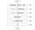
図4は、実施形態における軟判定装置4が実行する処理の流れの第1の例を示すフローチャートである。より具体的には、図4は、第1軟判定処理を実行する軟判定装置4が実行する処理の流れの一例を示すフローチャートである。
制御部40が、記憶部42の記憶する推定伝達関数と、インタフェース部41の取得した受信信号と、を取得する(ステップS101)。次に制御部40が、ブランチメトリック推定処理を実行する(ステップS102)。次に制御部40が、パスメトリック推定処理を実行する(ステップS103)。
次に制御部40が、ビット尤度推定処理を実行する(ステップS104)。制御部40は、ステップS104の処理で推定された尤度を、送信信号の(n+1)番目のシンボルに対する軟判定の結果として取得する。次に制御部40は、インタフェース部41の動作を制御して、ステップS104で推定された尤度をインタフェース部41に出力させる(ステップS105)。
図5は、実施形態における軟判定装置4が実行する処理の流れの第2の例を示すフローチャートである。より具体的には、図5は、第2軟判定処理を実行する軟判定装置4が実行する処理の流れの一例を示すフローチャートである。
制御部40が、記憶部42の記憶する推定伝達関数と、インタフェース部41の取得した受信信号と、を取得する(ステップS201)。次に制御部40が、硬判定処理を実行する(ステップS202)。次に制御部40が、尤度推定処理を実行する(ステップS203)。
次に制御部40が、違い取得処理を実行する(ステップS204)。制御部40は、ステップS204の処理で取得された尤度違いを、送信信号の(n+1)番目のシンボルに対する軟判定の結果として取得する。次に制御部40は、インタフェース部41の動作を制御して、ステップS204で推定された尤度違いをインタフェース部41に出力させる(ステップS205)。
このように、第2軟判定処理を実行する軟判定装置4は、シンボル多値度がmの送信信号、の(n+1)番目のシンボルである主シンボルに対する軟判定を行う。そして第2軟判定処理を実行する軟判定装置4は、制御部40を備える。制御部40は、送信信号が伝搬する伝送路2の伝達関数の予め得られた推定結果である推定伝達関数と、送信信号の受信の結果である受信信号と、に基づき、ビタビ・アルゴリズムによる硬判定を行う硬判定処理を実行する。制御部40は、(n+1)番目のシンボルの候補ごとに硬判定処理の結果と推定伝達関数と受信信号とに基づいて各候補の尤度を推定する尤度推定処理を実行する。制御部40は、候補のうちk番目(kは1以上m以下の整数)のビットが所定のビットである候補の尤度と、候補のうちk番目のビットが所定のビットでは無い候補の尤度と、の違いを取得する違い取得処理を実行する。制御部40は、取得した違いを、軟判定の結果として出力する。
<実験結果>
軟判定装置4を用いた実験の結果の一例を説明する。実験では、軟判定装置4を用いた実験の効果を評価するための比較対象の実験も行われた。比較対象の実験で用いられた技術は、軟判定装置4を用いない技術(以下「比較対象技術」という。)であった。より具体的には、比較対象技術は、伝達関数の逆関数を受信信号に作用させることで主シンボルを推定する技術である。
軟判定装置4を用いた実験の結果の一例を説明する。実験では、軟判定装置4を用いた実験の効果を評価するための比較対象の実験も行われた。比較対象の実験で用いられた技術は、軟判定装置4を用いない技術(以下「比較対象技術」という。)であった。より具体的には、比較対象技術は、伝達関数の逆関数を受信信号に作用させることで主シンボルを推定する技術である。
まず実験において用いられた光伝送システム100の一例を説明する。
実験において送信機1では、ユーザが伝送したい内容を示すデジタル信号、がアナログ信号に変換された。実験における変換は、128Gsample/s、65GHzの変換であった。実験において送信機1では、変換により得られたアナログ信号が増幅器によって増幅された。
実験において送信機1は、波長1310nmのレーザ光を増幅後のアナログ信号によって変調した結果、を光信号として出力した。変調方式は、PAM4であった。送信機1の出力した光信号は、伝送路2に入射し伝送路2を伝搬した。
実験において伝送路2は、長さ10kmのシングルモードファイバであった。伝送路2の波長分散は、波長1310nmにおいて、-8ps/nmであった。
実験において受信機3は可変光減衰器を備えており、受信機3では伝送路2から出射された光信号のパワーが可変光減衰器によって減衰された。受信機3は、可変光減衰器によるパワーの減衰後の光信号をフォトダイオードで電気信号に変換した。フォトダイオードの帯域幅は50GHzであった。
受信機3では、フォトダイオードにより得られた電気信号が増幅された後、デジタル信号に変換された。デジタル信号への変換は、160Gsample/s、63GHzの変換であった。変換後の信号は受信信号の一例であり、実験における受信信号の一例であった。
実験において軟判定装置4は、このようにして得られた受信信号を取得した。実験において軟判定装置4の備える制御部40は、第1軟判定処理を実行し、第1軟判定処理によって推定された尤度を軟判定の結果として取得した。実験において制御部40は、より具体的には、第1軟判定処理の実行により、式(1)で表される尤度を推定した。
図6は、実施形態における実験結果の一例を示す第1の図である。より具体的には、図6は、比較対象技術を用いた実験結果の一例を示す図である。図6の横軸は、周波数を示す。図6の縦軸は損失を示す。図6は、比較対象技術を用いた場合、周波数60GHz近傍で損失が大きくなることを示す。
図7は、実施形態における実験結果の一例を示す第2の図である。図7の横軸は、ROP(Received Optical Power)を示す。図7の縦軸は、規格一般化相互情報量(NGMI : Normalized General Mutual Information)を示す。
“MLSE(NGMI)”(Maximum Likelihood Sequence Estimation)が軟判定装置4を用いて第1軟判定処理を実行し式(1)で表される尤度を推定した結果を、NGMIの値で示す。“FFE(NGMI)”(Feed-Forward Equalizer)は比較対象技術を用いた結果をNGMIの値で示す。図7は、比較対象技術よりも軟判定装置4を用いて第1軟判定処理を実行し式(1)で表される尤度を推定した方が、NGMIが高いことを意味する。
図7は、軟判定装置4による軟判定の結果を用いることで、比較対象技術よりも高い精度で主シンボルが推定されることを示す。
<軟判定装置4が奏する効果の説明>
比較対象技術は、上述したように、伝達関数の逆関数を受信信号に作用させることで主シンボルを推定する。逆関数を作用させる場合、伝送路2で信号に付与された雑音までも増幅されてしまう。一方、軟判定装置4であれば伝達関数の逆関数は用いないので、雑音が増幅されてしまうことは無い。そのため、軟判定装置4は、比較対象技術よりも高い精度で主シンボルを推定することができる。
比較対象技術は、上述したように、伝達関数の逆関数を受信信号に作用させることで主シンボルを推定する。逆関数を作用させる場合、伝送路2で信号に付与された雑音までも増幅されてしまう。一方、軟判定装置4であれば伝達関数の逆関数は用いないので、雑音が増幅されてしまうことは無い。そのため、軟判定装置4は、比較対象技術よりも高い精度で主シンボルを推定することができる。
このように構成された軟判定装置4は、第1軟判定処理又は第2軟判定処理を実行する。そのため、伝達関数の逆関数を用いることなく軟判定の結果を得るので、軟判定装置4は、送信信号のシンボルをより高精度に推定することができる。
<第1実施形態の変形例>
なお、上述の式(1)、式(4)、式(7)、式(8)には、伝送路2で光信号に付与される雑音の分布の標準偏差σが含まれているが、伝送路2で光信号に付与される雑音の分布の標準偏差σの値は予め定められた値であってもよいし、予め定められた所定の値でなくてもよい。
例えば標準偏差σの値は、正解データに対して推定伝達関数を作用させた結果と受信信号との差分に基づいて得られてもよい。正解データは、送信信号の正解を示すデータである。したがって例えば標準偏差σは以下の式(12)が表す処理で得られてもよい。


式(13)におけるxdは、正解データが示す送信信号のd番目のシンボルを示す。式(13)のlは推定伝達関数の記憶長を意味し、一方で、式(12)のeは正解データが示す送信信号の開始の位置を示す。開始の位置とは、使用する正解データにおける時間軸方向の位置を示す。Dは標準偏差σの算出に用いられたシンボル数を表す。dは、使用する正解データにおける時間インデックスを意味する。したがって、式(12)はD個の推定雑音の平均値を標準偏差σとして取得する処理を表す。推定雑音とは、正解データに対して推定伝達関数を作用させた結果と受信信号との二乗誤差である。
例えば標準偏差σの値は、硬判定処理の結果に対して推定伝達関数を作用させた結果と受信信号との差分に基づいて得られてもよい。したがって例えば標準偏差σは以下の式(14)が表す処理で得られてもよい。


式(15)におけるx´dは、硬判定処理の結果が示す送信信号のd番目のシンボルを示す。式(15)のlは推定伝達関数の記憶長を意味し、一方で、式(14)のeは硬判定処理の結果が示す送信信号の開始の位置を示す。開始の位置とは、硬判定処理結果における時間軸方向の位置を示す。Dは標準偏差σの算出に用いられたシンボル数を表す。dは、使用する硬判定結果における時間インデックスを意味する。したがって、式(14)はD個の推定雑音の平均値を標準偏差σとして取得する処理を表す。
例えば標準偏差σの値は、NGMIを最大にする、という条件を満たす値であってもよい。NGMIは、例えば以下の式(16)で定義される量である。



m´は送信信号ビット数を表す。したがってm´は、例えば変調方式がPAM4の場合は、log2m´=2である。Nは、CrossEntropyの算出に用いられたシンボルの数を表す。
なお、軟出力の値(すなわち、軟判定の結果)は、プラス側又はマイナス側に発散する場合がある。プログラム言語によっては、発散すると値を出さないものが存在する。そこで、値が出ない事態を回避するため、送信信号の(n+1)番目のシンボルに対する軟判定を行う処理では、予め軟出力の値の上限又は下限が定められていてもよい。
なお、軟判定装置4は、ネットワークを介して通信可能に接続された複数台の情報処理装置を用いて実装されてもよい。この場合、軟判定装置4が備える各機能部は、複数の情報処理装置に分散して実装されてもよい。
なお、軟判定装置4の各機能の全て又は一部は、ASIC(Application Specific Integrated Circuit)やPLD(Programmable Logic Device)やFPGA(Field Programmable Gate Array)等のハードウェアを用いて実現されてもよい。プログラムは、コンピュータ読み取り可能な記録媒体に記録されてもよい。コンピュータ読み取り可能な記録媒体とは、例えばフレキシブルディスク、光磁気ディスク、ROM、CD-ROM等の可搬媒体、コンピュータシステムに内蔵されるハードディスク等の記憶装置である。プログラムは、電気通信回線を介して送信されてもよい。
(第2実施形態)
第2実施形態では、トレリス図における後ろ向き演算(残存パスの遡り)によるシンボル判定結果(硬判定結果)と、前向き演算(パスメトリックの算出と残存パス選択)によるシンボル判定結果とが異なっている場合には、残存パス以外のパスが示すパスメトリックも必要となる複雑な軟判定出力のための後ろ向き演算による軟判定結果を、簡易な演算による所定の軟判定結果で代替するという点が、第1実施形態との主な差分である。第2実施形態では、第1実施形態との差分を中心に説明する。
第2実施形態では、トレリス図における後ろ向き演算(残存パスの遡り)によるシンボル判定結果(硬判定結果)と、前向き演算(パスメトリックの算出と残存パス選択)によるシンボル判定結果とが異なっている場合には、残存パス以外のパスが示すパスメトリックも必要となる複雑な軟判定出力のための後ろ向き演算による軟判定結果を、簡易な演算による所定の軟判定結果で代替するという点が、第1実施形態との主な差分である。第2実施形態では、第1実施形態との差分を中心に説明する。
図8は、実施形態における制御部40の構成例を示す図である。制御部40は、伝達関数推定部401と、ブランチメトリック処理部402と、パスメトリック処理部403と、硬判定出力部404と、軟判定出力部405とを備える。
以下では、数式又は関数(以下「数式等」という。)において文字の上に付されている記号は、文字の前に記載される。例えば、数式等において文字の上に付されている記号「^」は、以下では文字「H」の前に「^H」のように記載される。
伝達関数推定部401は、式(19)のように推定伝達関数「^H」を算出する。

ブランチメトリック処理部402は、式(20)のようにブランチメトリック「b」を算出する。

パスメトリック処理部403は、式(21)のようにパスメトリック「p」を算出する。

硬判定出力部404は、各状態「s」のパスメトリック「p」を、時間インデックスごとに比較する。硬判定出力部404は、パスメトリック「p」の比較結果に基づいて、時間インデックス「n」における「ml」個の状態「s」のパスメトリックのうちから、最小パスメトリックを選択する。選択された最小パスメトリックの演算に使用されたブランチで構成された時間方向の道は、「残存パス」と呼ばれる。
トレリス図の残存パスを時間方向(状態遷移方向)とは逆の方向に遡るための起点としていずれの状態「s」が選択されたとしても、同じパスを遡るようになる。同じパスを遡るようになることは、「後ろ向き演算によるパスのマージ」と呼ばれる。マージされたパスを遡った先(以下「遡り先」という。)の状態に対応するシンボルが、シンボルの判定結果として出力される。シンボルの判定結果は、硬判定結果(硬判定の出力)に相当する。
硬判定出力部404は、トレリス図において、後ろ向き演算による硬判定結果「x’n-a」を生成する。シンボルの判定結果は、式(22)のように表される。

ここで、「a」は、状態遷移方向とは逆の方向にパスを遡る回数(遡り数)を表す。「sj」は、遡り先「j」における状態を表す。
また、硬判定出力部404は、トレリス図において、前向き演算による硬判定結果「x’’n-a」を生成する。時間インデックス「n」における最小パスメトリックを持つ状態が「sj」である場合、前向き演算(パスメトリックの算出と残存パス選択)の結果として判定されたシンボル「x’’n」は、式(23)のように表される。なお、式(23)の状態Sjの時間インデックスは、式(22)の状態Sjの時間インデックスとは異なる。このため、式(23)の左辺と式(22)の左辺とはイコール関係にはならない点に留意すべきである。

この判定されたシンボル「x’’n」は、後ろ向き演算(残存パスの遡り)が用いられずに、前向き演算(パスメトリックの算出と残存パス選択)のみが用いられたことによって得られた判定結果である。ここで、最も尤もらしいシンボル候補の系列長の系列推定しか出来ていないので、後ろ向き演算による遡り数を含む系列長の系列推定の効果は得られない。
このため、同じ時間インデックス「n-a」であっても、後ろ向き演算によるシンボル判定結果「x’n-a」と、前向き演算によるシンボル判定結果「x’’n-a」とが異なる場合がある。また、異なる場合には、前向き演算によるシンボル判定結果「x’’n-a」よりも、後ろ向き演算によるシンボル判定結果「x’n-a」のほうが正確である可能性が高い。
第1実施形態において例示された式(1)では、前向き演算によるパスメトリックの情報に基づいて、対数尤度比「λM,n」が算出されている。このため、後ろ向き演算のシンボル判定結果「x’n-a」と前向き演算のシンボル判定結果「x’’n-a」とが異なる場合、前向き演算によるパスメトリックの情報に基づいて推定された対数尤度比「λ」の精度が高くない可能性がある。
そこで第2実施形態では、軟判定出力部405は、トレリス図におけるパスの遡り(後ろ向き演算)の効果を、簡易な計算によって、近似的に取り入れる。すなわち、軟判定出力部405は、複雑な後ろ向き演算の軟判定結果を、簡易な演算の軟判定結果で代替する。この簡易な計算の複雑さは、例えば、硬判定の最尤系列推定(MLSE)において用いられるビタビ・アルゴリズムの複雑さと同程度である。
対数尤度比「λ’k,n」は、式(25)を用いて、式(24)のように表される。式(24)の演算は、本質的に式(7)と同じになる。


ここで、「n」は、時間インデックス(1≦n≦N)を表す。「k」は、時間インデックス「n」におけるシンボル判定結果の何番目(1≦k≦m)のビットであるかを表す。「c’k,n」は、時間インデックス「n」におけるシンボル判定結果「x’n」のk番目のビット(0又は1)を表す。なお、「c’’k,n」は、時間インデックス「n」におけるシンボル判定結果「x’’n」のk番目のビット(0又は1)を表す。
軟判定出力部405は、予め定められた正の定数「A」を、例えばメモリ92から取得する。この定数「A」は、例えば、正の変数が所定間隔で変更された結果に応じて規格一般化相互情報量(NGMI)が最大になるように、予め定められる。例えば、0.001から1.000までの値を採る変数が0.001間隔で変更されることによって、変数の値ごとに対数尤度比「λ」が算出される。規格一般化相互情報量が最大になる場合における変数の値が、正の定数「A」と予め定められる。
軟判定出力部405は、後ろ向き演算のシンボル判定結果「x’n-a」と、前向き演算のシンボル判定結果「x’’n-a」とを、ビットごとに比較する。軟判定出力部405は、シンボル判定結果「x’n-a」とシンボル判定結果「x’’n-a」とが同じである場合、軟判定出力部405は、軟判定結果「λk,n-a」として、対数尤度比「λ’k,n-a」を出力する。
軟判定出力部405は、シンボル判定結果「x’n-a」とシンボル判定結果「x’’n-a」とが異なっている場合、符号関数「sgn」を用いて、式(24)の対数尤度比「λ’k,n」の符号を取得する。軟判定出力部405は、式(24)の対数尤度比「λ’k,n」の符号を取得する代わりに、式(1)の対数尤度比「λk,n」の符号を取得してもよい。軟判定出力部405は、対数尤度比「λ’k,n」の符号とは逆の符号と、予め定められた定数「A」と、雑音の分布の標準偏差「σ」とに基づいて、新たな軟判定結果「λk,n-a」を算出する。
シンボル判定結果「x’n-a」とシンボル判定結果「x’’n-a」とが同じ場合における軟判定結果「λk,n-a」(対数尤度比)と、シンボル判定結果「x’n-a」とシンボル判定結果「x’’n-a」とが異なっている場合における新たな軟判定結果「λk,n-a」(変更された対数尤度比)とのそれぞれは、式(26)のように表される。

図9は、実施形態における軟判定装置4が実行する処理の流れの第3の例を示すフローチャートである。制御部40が、記憶部42の記憶する推定伝達関数と、インタフェース部41の取得した受信信号と、を取得する(ステップS301)。次に制御部40が、ブランチメトリック推定処理を実行する(ステップS302)。次に制御部40が、パスメトリック推定処理を実行する(ステップS303)。
制御部40が、硬判定処理を実行することによって、後ろ向き演算のシンボル判定結果と、前向き演算のシンボル判定結果とを生成する(ステップS304)。制御部40が、後ろ向き演算のシンボル判定結果と、前向き演算のシンボル判定結果と、予め定められた定数「A」とに基づいて、ビット尤度推定処理を実行する(ステップS305)。制御部40は、ステップS305の処理において推定された尤度を、軟判定の結果として取得する。制御部40は、インタフェース部41の動作を制御して、ステップS305において推定された尤度「λk,n-a」を、インタフェース部41に出力させる(ステップS306)。
以上のように、制御部40は、送信信号の(n+a)番目(例えば、a=1)からn番目の順に演算したことによるn番目のシンボルの判定結果「x’n」と、送信信号のn番目から(n+a)番目の順に演算したことによるn番目のシンボルの判定結果「x’’n」とが異なる場合、推定された尤度の符号(sgn(λ’k,n))とは逆の符号「-」と、予め定められた定数「A」と、標準偏差「σ」とに基づいて、尤度「λk,n」を変更する。予め定められた定数「A」は、分布の正のピークを示す尤度「P」と、標準偏差「σ」とに基づいて、「2σ2P」と定められる。
このように第2実施形態では、シンボル判定結果「x’n-a」とシンボル判定結果「x’’n-a」とが同じである場合と、シンボル判定結果「x’n-a」とシンボル判定結果「x’’n-a」とが異なる場合とで、ビットごとの対数尤度比(ビット尤度)「λk,n-a」を異ならせる。これによって、規格一般化相互情報量(NGMI)をより改善することが可能である。
また、第1実施形態と比較して、送信信号のシンボルをより高精度に推定することが可能となる。
<第2実施形態の変形例>
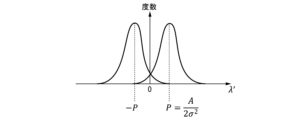
図10は、実施形態におけるビット尤度ヒストグラムの一例を示す図である。軟判定出力部405は、予め定められた正の定数「A」を、例えばメモリ92から取得する。式(26)に例示されているように、軟判定結果の絶対値は、「A/2σ2」と表される。
図10は、実施形態におけるビット尤度ヒストグラムの一例を示す図である。軟判定出力部405は、予め定められた正の定数「A」を、例えばメモリ92から取得する。式(26)に例示されているように、軟判定結果の絶対値は、「A/2σ2」と表される。
ビット尤度ヒストグラムの分散「σ2」に関係なく、正の定数「A」の最適値が伝送系及び復調方法ごとに一定になる傾向がある。また、正の定数「A」の最適値は、ビット尤度ヒストグラムのピークを示す正の尤度「P(=A/2σ2)」に近い。そこで、その尤度「P(=A/2σ2)」に基づいて、正の定数「A」が予め定められてもよい。
<実験結果>
軟判定装置4を用いた実験の結果の一例を説明する。
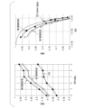
図11は、実施形態における実験結果の一例を示す第3の図である。図11では、シンボル多値度「M」は、一例として4である。記憶長「d」は、一例として5である。遡り数「T」は、一例として20である。第2実施形態における予め定められた正の定数「A」は、一例として0.018である。
軟判定装置4を用いた実験の結果の一例を説明する。
図11は、実施形態における実験結果の一例を示す第3の図である。図11では、シンボル多値度「M」は、一例として4である。記憶長「d」は、一例として5である。遡り数「T」は、一例として20である。第2実施形態における予め定められた正の定数「A」は、一例として0.018である。
第1実施形態の対数尤度比「λ」の算出に必要とされるパスメトリックの個数「Md」は、一例として1024である。第2実施形態の対数尤度比「λ」の算出に必要とされるパスメトリックの個数「2Md」は、一例として1024である。FFE方式の対数尤度比「λ」の算出に必要とされるパスメトリックの個数「Md+1T」は、一例として81920である。
図11における左側のグラフは、FFE方式と、第1実施形態におけるNL-MLSE方式と、第2実施形態におけるNL-MLSE方式とについて、受信光強度(ROP)と、規格一般化相互情報量(NGMI)との関係が示されている。
第1実施形態におけるNL-MLSE方式の受信光強度と、第2実施形態におけるNL-MLSE方式の受信光強度とのいずれでも、FFE方式よりも高い規格一般化相互情報量が達成されている。ROPが3dBmである場合、第1実施形態では、規格一般化相互情報量が約18%改善される。また、第2実施形態では、規格一般化相互情報量が約22%改善される。
図11における右側のグラフは、FFE方式と、第1実施形態におけるNL-MLSE方式と、第2実施形態におけるNL-MLSE方式とについて、符号誤り率(BER : Bit Error Rate)と、規格一般化相互情報量(NGMI)との関係が示されている。右側のグラフにおいて、FFE方式の結果と重なる破線は、加法性白色ガウス雑音(AWGN)チャネルの理論曲線を表す。理論曲線が表す性能は、NL-MLSE方式と同じBERが得られる場合の、演算量が非常に多いソフト出力ビタビ・アルゴリズム(SOVA : Soft Output Viterbi Algorithm)の性能に相当する。
FFE方式では、符号誤り率「0.8」を達成することができない。これに対して、第1実施形態におけるNL-MLSE方式では、符号誤り率「0.931」を達成することができる。また、第2実施形態におけるNL-MLSE方式では、符号誤り率「0.962」を達成することができる。このように、第2実施形態における光伝送システム100は、ソフト出力ビタビ・アルゴリズムによる規格一般化相互情報量「0.985」に近い性能を、より少ない演算量で実現することができる。
以上、この発明の実施形態について図面を参照して詳述してきたが、具体的な構成はこの実施形態に限られるものではなく、この発明の要旨を逸脱しない範囲の設計等も含まれる。
100…光伝送システム、 1…送信機、 2…伝送路、 3…受信機、 4…軟判定装置、 40…制御部、 41…インタフェース部、 42…記憶部、 91…プロセッサ、 92…メモリ、401…伝達関数推定部、402…ブランチメトリック処理部、403…パスメトリック処理部、404…硬判定出力部、405…軟判定出力部
Claims (7)
- シンボル多値度がm(mは2以上の整数)の送信信号、の(n+1)番目(nは1以上N以下の整数。Nは1以上の整数)のシンボルである主シンボルに対する軟判定を行う軟判定装置であって、
前記送信信号が伝搬する伝送路の伝達関数の予め得られた推定結果である推定伝達関数と、前記送信信号の受信の結果である受信信号と、に基づき、ビタビ・アルゴリズムで得られる距離であり所定の距離関数が示す距離であり前記送信信号のn番目のシンボルから(n+1)番目のシンボルの各候補に遷移する尤度を示す距離であるブランチメトリックを推定するブランチメトリック推定処理と、
前記ブランチメトリック推定処理の結果に基づき、ビタビ・アルゴリズムで得られる距離であり所定の距離関数が示す距離であり前記送信信号の(n+1)番目のシンボルの各候補が前記送信信号のシンボルである尤度を示す距離と、前記送信信号の1番目からn番目の残存パスの距離との合計であるパスメトリックを推定するパスメトリック推定処理と、
前記パスメトリック推定処理によって得られた前記送信信号の(n+1)番目のシンボルの各候補のパスメトリックを用い、前記送信信号の(n+1)番目のシンボルの各候補のパスメトリック以外のパスメトリックは用いずに、前記送信信号の(n+1)番目のシンボルにおけるk番目(kは1以上m以下の整数)のビットが所定のビットである尤度を推定するビット尤度推定処理と、
を実行する制御部、
を備え、
前記制御部は、前記ビット尤度推定処理で推定された尤度を、前記軟判定の結果として取得する、
軟判定装置。 - 前記制御部は、前記伝送路で前記送信信号に付与される雑音の分布の標準偏差、も用いて、前記尤度を推定する、
請求項1に記載の軟判定装置。 - 前記標準偏差は、送信信号の正解を示す正解データに対して前記推定伝達関数を作用させた結果と前記受信信号との差分に基づいて得られる、
請求項2に記載の軟判定装置。 - 前記制御部は、前記送信信号の(n+1)番目からn番目の順に演算したことによるn番目のシンボルの判定結果と、前記送信信号のn番目から(n+1)番目の順に演算したことによるn番目のシンボルの判定結果とが異なる場合、推定された前記尤度の符号とは逆の符号と、予め定められた定数と、前記標準偏差とに基づいて、前記尤度を変更する、
請求項2に記載の軟判定装置。 - 前記予め定められた定数は、前記分布の正のピークを示す前記尤度と、前記標準偏差とに基づいて定められる、
請求項4に記載の軟判定装置。 - シンボル多値度がm(mは2以上の整数)の送信信号、の(n+1)番目(nは1以上N以下の整数。Nは1以上の整数)のシンボルである主シンボルに対する軟判定を行う軟判定方法であって、
前記送信信号が伝搬する伝送路の伝達関数の予め得られた推定結果である推定伝達関数と、前記送信信号の受信の結果である受信信号と、に基づき、ビタビ・アルゴリズムで得られる距離であり所定の距離関数における距離であり前記送信信号のn番目のシンボルから(n+1)番目のシンボルの各候補に遷移する尤度を示す距離であるブランチメトリックを推定するブランチメトリック推定処理と、
前記ブランチメトリック推定処理の結果に基づき、ビタビ・アルゴリズムで得られる距離であり所定の距離関数における距離であり前記送信信号の(n+1)番目のシンボルの各候補が前記送信信号のシンボルである尤度を示す距離と、前記送信信号の1番目からn番目の残存パスの距離との合計であるパスメトリックを推定するパスメトリック推定処理と、
前記パスメトリック推定処理によって得られた前記送信信号の(n+1)番目のシンボルの各候補のパスメトリックを用い、前記送信信号の(n+1)番目のシンボルの各候補のパスメトリック以外のパスメトリックは用いずに、前記送信信号の(n+1)番目のシンボルにおけるk番目(kは1以上m以下の整数)のビットが所定のビットである尤度を推定するビット尤度推定処理と、
を実行する制御ステップ、
を有し、
前記制御ステップは、前記ビット尤度推定処理で推定された尤度を、前記軟判定の結果として取得する、
軟判定方法。 - 請求項1から5のいずれか一項に記載の軟判定装置としてコンピュータを機能させるためのプログラム。
Priority Applications (2)
| Application Number | Priority Date | Filing Date | Title |
|---|---|---|---|
| US19/099,434 US20260039317A1 (en) | 2022-08-09 | 2023-01-17 | Soft decision apparatus, soft decision method and program |
| JP2024540243A JP7839430B2 (ja) | 2022-08-09 | 2023-01-17 | 軟判定装置、軟判定方法及びプログラム |
Applications Claiming Priority (2)
| Application Number | Priority Date | Filing Date | Title |
|---|---|---|---|
| PCT/JP2022/030392 WO2024034003A1 (ja) | 2022-08-09 | 2022-08-09 | 軟判定装置、軟判定方法及びプログラム |
| JPPCT/JP2022/030392 | 2022-08-09 |
Publications (1)
| Publication Number | Publication Date |
|---|---|
| WO2024034154A1 true WO2024034154A1 (ja) | 2024-02-15 |
Family
ID=89851212
Family Applications (2)
| Application Number | Title | Priority Date | Filing Date |
|---|---|---|---|
| PCT/JP2022/030392 Ceased WO2024034003A1 (ja) | 2022-08-09 | 2022-08-09 | 軟判定装置、軟判定方法及びプログラム |
| PCT/JP2023/001097 Ceased WO2024034154A1 (ja) | 2022-08-09 | 2023-01-17 | 軟判定装置、軟判定方法及びプログラム |
Family Applications Before (1)
| Application Number | Title | Priority Date | Filing Date |
|---|---|---|---|
| PCT/JP2022/030392 Ceased WO2024034003A1 (ja) | 2022-08-09 | 2022-08-09 | 軟判定装置、軟判定方法及びプログラム |
Country Status (3)
| Country | Link |
|---|---|
| US (1) | US20260039317A1 (ja) |
| JP (1) | JP7839430B2 (ja) |
| WO (2) | WO2024034003A1 (ja) |
Citations (4)
| Publication number | Priority date | Publication date | Assignee | Title |
|---|---|---|---|---|
| JP2002537688A (ja) * | 1999-02-09 | 2002-11-05 | ルーセント テクノロジーズ インコーポレーテッド | 経路指向復号器による符号化または非符号化変調の終了 |
| JP2003273751A (ja) * | 2002-03-12 | 2003-09-26 | Matsushita Electric Ind Co Ltd | ビット尤度算出方法及び復調装置 |
| JP4188079B2 (ja) * | 2000-07-24 | 2008-11-26 | 三菱電機株式会社 | 無線通信用受信装置および受信方法 |
| WO2022029835A1 (ja) * | 2020-08-03 | 2022-02-10 | 日本電信電話株式会社 | 光信号復調器、制御方法およびプログラム |
-
2022
- 2022-08-09 WO PCT/JP2022/030392 patent/WO2024034003A1/ja not_active Ceased
-
2023
- 2023-01-17 JP JP2024540243A patent/JP7839430B2/ja active Active
- 2023-01-17 US US19/099,434 patent/US20260039317A1/en active Pending
- 2023-01-17 WO PCT/JP2023/001097 patent/WO2024034154A1/ja not_active Ceased
Patent Citations (4)
| Publication number | Priority date | Publication date | Assignee | Title |
|---|---|---|---|---|
| JP2002537688A (ja) * | 1999-02-09 | 2002-11-05 | ルーセント テクノロジーズ インコーポレーテッド | 経路指向復号器による符号化または非符号化変調の終了 |
| JP4188079B2 (ja) * | 2000-07-24 | 2008-11-26 | 三菱電機株式会社 | 無線通信用受信装置および受信方法 |
| JP2003273751A (ja) * | 2002-03-12 | 2003-09-26 | Matsushita Electric Ind Co Ltd | ビット尤度算出方法及び復調装置 |
| WO2022029835A1 (ja) * | 2020-08-03 | 2022-02-10 | 日本電信電話株式会社 | 光信号復調器、制御方法およびプログラム |
Also Published As
| Publication number | Publication date |
|---|---|
| WO2024034003A1 (ja) | 2024-02-15 |
| JPWO2024034154A1 (ja) | 2024-02-15 |
| US20260039317A1 (en) | 2026-02-05 |
| JP7839430B2 (ja) | 2026-04-02 |
Similar Documents
| Publication | Publication Date | Title |
|---|---|---|
| EP3577765B1 (en) | Soft output decoding of polar codes using successive cancelation list (scl) decoding | |
| US7206363B2 (en) | Method and apparatus for delayed recursion decoder | |
| EP0771079A2 (en) | Data transmission device | |
| CN102439855B (zh) | 用于在缩减状态均衡器中生成软比特值的方法和设备 | |
| CN107453807B (zh) | 一种大气光通信信道模型的极化方法、装置及电子设备 | |
| US7380199B2 (en) | Method and apparatus for precomputation and pipelined selection of branch metrics in a reduced-state Viterbi detector | |
| EP3451539A1 (en) | Optical receiver, optical transmission device, and method for optical receiver | |
| JP7839430B2 (ja) | 軟判定装置、軟判定方法及びプログラム | |
| US6701483B1 (en) | Fast search-based decoding scheme | |
| WO2022029835A1 (ja) | 光信号復調器、制御方法およびプログラム | |
| WO2025017868A1 (ja) | 軟判定装置、軟判定方法及びプログラム | |
| US7512868B2 (en) | Method for processing a signal using an approximate map algorithm and corresponding uses | |
| Plotnikov et al. | Spectral efficiency comparison between FTN signaling and optimal PR signaling for low complexity detection algorithm | |
| US7653154B2 (en) | Method and apparatus for precomputation and pipelined selection of intersymbol interference estimates in a reduced-state Viterbi detector | |
| US8976912B1 (en) | Decoding apparatus and decoding method | |
| Fu et al. | Dual-RNN based polar decoder with tanh-modified LLR over FSO turbulence channel | |
| WO2025154205A1 (ja) | 軟判定装置、軟判定方法及びプログラム | |
| Zeitler | Low-precision analog-to-digital conversion and mutual information in channels with memory | |
| US11205131B2 (en) | Sequence detection | |
| KR100912073B1 (ko) | 연판정 디코딩 방법 및 연판정 디코딩 장치 | |
| US12556203B2 (en) | Symbol judgement apparatus, symbol judgement method and program | |
| Liberatori et al. | Soft distance metric decoding of polar codes | |
| Islam et al. | Performance comparison of Rate ½ Convolutional Codes with BPSK on Rayleigh and AWGN channels for Memory or Memory less condition | |
| US20260025209A1 (en) | Encoding and decoding using probabilistic shaping | |
| US20120233526A1 (en) | Generation of soft bit metrics for differentially encoded quadrature phase shift keying (qpsk) |
Legal Events
| Date | Code | Title | Description |
|---|---|---|---|
| 121 | Ep: the epo has been informed by wipo that ep was designated in this application |
Ref document number: 23852141 Country of ref document: EP Kind code of ref document: A1 |
|
| WWE | Wipo information: entry into national phase |
Ref document number: 2024540243 Country of ref document: JP |
|
| NENP | Non-entry into the national phase |
Ref country code: DE |
|
| 122 | Ep: pct application non-entry in european phase |
Ref document number: 23852141 Country of ref document: EP Kind code of ref document: A1 |