WO2020162188A1 - 潜在変数最適化装置、フィルタ係数最適化装置、潜在変数最適化方法、フィルタ係数最適化方法、プログラム - Google Patents
潜在変数最適化装置、フィルタ係数最適化装置、潜在変数最適化方法、フィルタ係数最適化方法、プログラム Download PDFInfo
- Publication number
- WO2020162188A1 WO2020162188A1 PCT/JP2020/002205 JP2020002205W WO2020162188A1 WO 2020162188 A1 WO2020162188 A1 WO 2020162188A1 JP 2020002205 W JP2020002205 W JP 2020002205W WO 2020162188 A1 WO2020162188 A1 WO 2020162188A1
- Authority
- WO
- WIPO (PCT)
- Prior art keywords
- variable
- filter coefficient
- auxiliary
- cost
- optimization
- Prior art date
- Legal status (The legal status is an assumption and is not a legal conclusion. Google has not performed a legal analysis and makes no representation as to the accuracy of the status listed.)
- Ceased
Links
Images


Classifications
-
- H—ELECTRICITY
- H04—ELECTRIC COMMUNICATION TECHNIQUE
- H04R—LOUDSPEAKERS, MICROPHONES, GRAMOPHONE PICK-UPS OR LIKE ACOUSTIC ELECTROMECHANICAL TRANSDUCERS; ELECTRIC HEARING AIDS; PUBLIC ADDRESS SYSTEMS
- H04R3/00—Circuits for transducers
- H04R3/04—Circuits for transducers for correcting frequency response
-
- H—ELECTRICITY
- H04—ELECTRIC COMMUNICATION TECHNIQUE
- H04R—LOUDSPEAKERS, MICROPHONES, GRAMOPHONE PICK-UPS OR LIKE ACOUSTIC ELECTROMECHANICAL TRANSDUCERS; ELECTRIC HEARING AIDS; PUBLIC ADDRESS SYSTEMS
- H04R3/00—Circuits for transducers
- H04R3/005—Circuits for transducers for combining the signals of two or more microphones
-
- G—PHYSICS
- G06—COMPUTING OR CALCULATING; COUNTING
- G06F—ELECTRIC DIGITAL DATA PROCESSING
- G06F17/00—Digital computing or data processing equipment or methods, specially adapted for specific functions
- G06F17/10—Complex mathematical operations
- G06F17/18—Complex mathematical operations for evaluating statistical data, e.g. average values, frequency distributions, probability functions, regression analysis
-
- G—PHYSICS
- G10—MUSICAL INSTRUMENTS; ACOUSTICS
- G10L—SPEECH ANALYSIS TECHNIQUES OR SPEECH SYNTHESIS; SPEECH RECOGNITION; SPEECH OR VOICE PROCESSING TECHNIQUES; SPEECH OR AUDIO CODING OR DECODING
- G10L21/00—Speech or voice signal processing techniques to produce another audible or non-audible signal, e.g. visual or tactile, in order to modify its quality or its intelligibility
- G10L21/02—Speech enhancement, e.g. noise reduction or echo cancellation
- G10L21/0272—Voice signal separating
-
- H—ELECTRICITY
- H04—ELECTRIC COMMUNICATION TECHNIQUE
- H04R—LOUDSPEAKERS, MICROPHONES, GRAMOPHONE PICK-UPS OR LIKE ACOUSTIC ELECTROMECHANICAL TRANSDUCERS; ELECTRIC HEARING AIDS; PUBLIC ADDRESS SYSTEMS
- H04R5/00—Stereophonic arrangements
- H04R5/04—Circuit arrangements, e.g. for selective connection of amplifier inputs/outputs to loudspeakers, for loudspeaker detection, or for adaptation of settings to personal preferences or hearing impairments
-
- H—ELECTRICITY
- H04—ELECTRIC COMMUNICATION TECHNIQUE
- H04R—LOUDSPEAKERS, MICROPHONES, GRAMOPHONE PICK-UPS OR LIKE ACOUSTIC ELECTROMECHANICAL TRANSDUCERS; ELECTRIC HEARING AIDS; PUBLIC ADDRESS SYSTEMS
- H04R2430/00—Signal processing covered by H04R, not provided for in its groups
- H04R2430/20—Processing of the output signals of the acoustic transducers of an array for obtaining a desired directivity characteristic
Definitions
- the present invention relates to a technique for optimizing a latent variable of a model to be optimized such as a filter coefficient in target sound enhancement.
- Beamforming using a microphone array is well known as a signal processing method that emphasizes only the sound coming from a specific direction and suppresses noise in the other direction. This method has been put to practical use in telephone conference systems, in-vehicle communication systems, smart speakers, etc.
- Most of the conventional methods for beamforming have derived the optimum filter by solving the cost function minimization problem under some constraints.
- the MVDR beamformer described in Non-Patent Document 1 can be obtained by using the power of the output signal as a cost function and minimizing it under the distortion-free characteristic constraint for the target sound source direction.
- a maximum likelihood (ML) beamformer is derived by minimizing the power of noise included in the output signal as a cost function.
- Other attempts have also been made to add additional constraints and cost terms to the cost function in order to improve the performance of the beamformer.
- the beamformer When applying the beamformer to the actual situation, if it is possible to have multiple characteristics at the same time, it is considered useful for application. For example, there may be situations in which a beamformer that maintains both high delay performance for speech and low delay characteristics is required.
- the demands on the characteristics of the beamformer can be theoretically modeled in the form of stochastic assumptions for auxiliary variables defined by the filter coefficients of the beamformer. For example, if there is prior knowledge that the sound to be emphasized is a human voice, it is reasonable to assume that the estimated signal follows a highly sparse distribution such as the Laplace distribution in the time frequency domain.
- an object of the present invention is to provide a technique for optimizing a latent variable using a cost function that simultaneously considers a plurality of stochastic assumptions.
- One embodiment of the present invention is a latent variable optimization device including an optimization unit for optimizing a latent variable ⁇ w * , wherein v j (1 ⁇ j ⁇ J) is calculated using a matrix D j and a vector b j.
- the cost term of auxiliary variable v j can be expressed using the probability distribution of auxiliary variable v j that is log-concave.
- the optimization unit optimizes the latent variable ⁇ w * by solving the cost function minimization problem including the sum of the cost terms of the auxiliary variables v j .
- FIG. 3 is a block diagram showing a configuration of a latent variable optimizing device 100 (filter coefficient optimizing device 100).
- 6 is a flowchart showing an operation of the latent variable optimizing device 100 (filter coefficient optimizing device 100).
- 3 is a block diagram showing the configuration of an optimization unit 120.
- FIG. 6 is a flowchart showing the operation of the optimizing unit 120.
- x y_z means that y z is a subscript to x
- x y_z means that y z is a subscript to x
- the filter coefficient is optimized (learned) by using the cost function designed based on the stochastic assumption for the filter coefficient itself and the auxiliary variable determined from the filter coefficient.
- the auxiliary variable is limited to that expressed as an affine transformation of the filter coefficient, but, for example, the estimated target sound, noise included in the output signal, the difference of the filter coefficient between adjacent frequency bins, etc. are in this category. included. If the assumed probability distributions for the filter coefficient and its auxiliary variable are all log-concave (log-concave), the joint distribution when the filter coefficient and auxiliary variable are considered to be independent of each other is also log-concave.
- Negative log-likelihood becomes a convex function, and the cost function optimization problem is reduced to a convex function optimization problem for auxiliary variables constrained by a linear relational expression.
- This optimization problem can be solved by using, for example, the Alternating Direction Method of Multipliers (ADMM), and the optimum filter coefficient can be efficiently calculated.
- ADMM Alternating Direction Method of Multipliers
- n bf,t represents a noise signal that is not assumed to be derived from a specific disturbing sound source (for example, noise caused by the performance of the microphone itself).
- h f ⁇ C M is an array manifold vector of the target sound source direction.
- the transfer function a f instead of the array manifold vector h f under the model like the equation (1), but it is difficult to know the transfer function accurately in practical use. Therefore, the array manifold vector h f is used in the definition of equation (3). If the beamformer can properly extract the target sound, it is expected that the estimated value e f of the non-target sound is mainly composed of the disturbing sound and the background noise.
- the estimated values of the target sound and the non-target sound can both be expressed as affine transformations of the filter coefficients, they are expressed as a conversion equation using the filter coefficients.
- the output value of the beamformer at the time frame t the estimated value of the target sound ⁇ y t (hereinafter referred to as the estimated target sound) and the estimated value of noise ⁇ e t (hereinafter referred to as the estimated noise and the estimated non-target sound) are respectively It is expressed in the form of affine transformation of the following filter coefficient ⁇ w * .
- the conventional beamforming optimization problem is described as a cost function minimization problem defined from the viewpoint of a probabilistic model.
- Equation (9) has been formulated as an optimization problem related to the variable ⁇ w *, and can be easily solved for a relatively simple example such as the MVDR beamformer described above, but the cost function is When it comes to complicated expressions, it is generally difficult to perform optimization as well. From this, it can be seen that the conventional method has two problems. First, the conventional methods tend to limit the assumed probability distributions for target sounds ⁇ y and non-target sounds ⁇ e to simple ones like the normal distribution. There is a point that is not always appropriate as a description of sound source distribution. Second, the cost function that can be used as a constraint on the filter coefficient ⁇ w * is also limited, and it is difficult to consider various stochastic assumptions at the same time.
- the new cost function for the beamforming optimization problem is expressed as the sum of various convex function terms. Further, the argument of each term, the auxiliary variable that can be defined as the filter coefficient ⁇ w * and (as estimated target sound ⁇ y t and the estimated noise ⁇ e t) newly introduced is the filter coefficient ⁇ w * affine transformation To do. ..
- the cost function satisfying these requirements is easy to solve the optimization problem. In other words, the cost function can be freely designed within the range that satisfies these requirements. The details will be described below.
- ⁇ v (v 1 T ,..., v J T ) T
- ⁇ D (D 1 T ,..., D J T ) T
- ⁇ b (b 1 T , ..., b J T ).
- the cost function L is also a convex function.
- the constraint that the cost term of the auxiliary variable v j is a convex function may seem strange at first glance, but this is actually the estimated target sound ⁇ y t in Eq. (6) or the estimated noise ⁇ e t in Eq. (7). It is nothing but the adoption of a log-concave one for the probability distribution of variables.
- the probability distribution being log-concave means that ⁇ 1 times the logarithm of the probability density function (negative log) is a convex function.
- the problem of equation (15) can be solved by dividing it into terms relating to filter coefficients and terms relating to auxiliary variables, and performing optimization alternately for each.
- Various concrete algorithms for solving this problem are known, and as an example, there is an algorithm adopting the alternating direction multiplier method (ADMM) (the algorithm will be described later).
- ADMM alternating direction multiplier method
- the target sound is a voice in the above-mentioned assumed situation. Since it is known that speech has a property of sparseness, it is considered that this known information can be utilized by designing a cost term in consideration of the assumption that the estimated target sound follows a sparse probability distribution. Therefore, the estimated target sound ⁇ y t is adopted as an auxiliary variable.
- the definition of the auxiliary variable ⁇ y t is the same as in equation (6). Then, it is assumed that the auxiliary variable ⁇ y t follows the Laplace distribution of the following equation.
- ⁇ (>0) is a constant parameter that determines the shape of the distribution.
- the Laplace distribution is often used to express the distribution of sparse variables, and is considered appropriate in the above hypothesized situation.
- the cost term L y of the auxiliary variable ⁇ y is -1 times the logarithm of the Laplace distribution.
- the estimated non-target sound ⁇ e t defined by equation (7) is introduced as an auxiliary variable.
- the non-objective sound which is mainly an interference sound, follows a normal distribution. That is, the auxiliary variable ⁇ e t is
- R f is the spatial correlation matrix for the non-target sound and can be estimated from the observed data. Rewriting the assumption of Eq. (18) into the form of the cost term for the auxiliary variable ⁇ e,
- a conventional wideband beamformer derives filter coefficients independently for each frequency bin, and does not consider the relationship between adjacent frequency bins.
- the frequency characteristic of discontinuity or non-smoothness in the frequency bin direction causes an impulse response with a long tail in the time domain.
- introduce a difference in the frequency bin direction of the filter coefficient as a new auxiliary variable and impose a cost term that makes these auxiliary variables (norm) small. Is considered to be effective. Specifically,
- Equation (20) is designed so that ⁇ f contains the information of the second derivative with respect to the frequency direction of the amplitude-phase characteristic of the filter.
- the cost term L ⁇ _f ( ⁇ f ) for the auxiliary variable ⁇ f is
- the cost function L is the sum of the cost terms by making the assumptions about the auxiliary variables such as Equation (18), Equation (16), and Equation (20).
- an image in which noise is superimposed on an image with a periodic pattern (hereinafter referred to as the original image) such as an image in which a large number of objects of the same shape are captured is given as input, and noise is removed from the image.
- the original image such as an image in which a large number of objects of the same shape are captured
- noise is removed from the image.
- N a matrix representing noise added to each pixel
- the matrix S is regarded as ⁇ w * in Equation (15), and the cost terms related to the auxiliary variables determined by the affine transformation of the matrix S and the matrix S are Make up.
- the cost term L s in Eq. (24) is a convex function.
- L D1 and L D2 are cost terms having the meaning of noise removal.
- the original image has a priori knowledge that it has a periodic structure, and auxiliary variables and cost terms that can make use of such priori knowledge are designed.
- the spatial frequency spectrum obtained by two-dimensional Fourier transform of the image is expected to have a sparse structure. Since the two-dimensional Fourier transform can be described as an affine transform, we decided to adopt the spatial frequency spectrum as auxiliary variables and design our own cost term to induce these auxiliary variables into sparse, and we believe that our objective will be achieved.
- the matrix S is the variable to be estimated, and the other variables are the auxiliary variables of the matrix S.
- FIG. 1 is a diagram showing an iterative algorithm for actually solving the convex constrained optimization problem with a linear constraint represented by Expression (15).
- This algorithm is based on ADMM, which is known as one of the algorithms that efficiently solves the problem of equation (15).
- ADMM is an algorithm that optimizes the dual problem of the original problem, and uses the dual variable u j having the same dimension as the auxiliary variable v j .
- the Cholesky factorization of the matrix ⁇ D H ⁇ D can make the calculation of multiplication by ( ⁇ D H ⁇ D) -1 which is necessary for updating efficient.
- the update rule of the auxiliary variable is obtained.
- This update rule is described as a proximity operator for each cost term.
- I represents an identity matrix
- effect The principle of the embodiment of the present invention is desired by interpreting the filter coefficient derivation of the beamformer as a cost function optimization problem and then imposing a constraint based on an individual cost term for the filter coefficient and its auxiliary variable.
- the purpose is to design a beamformer that has multiple characteristics.
- a cost function is configured in the framework of individually designing cost terms for these variables.
- Each cost term has the meaning of being a stochastic assumption, and particularly when imposing a log-concave stochastic assumption, it results in a linear constrained convex optimization problem, and it is relatively easy to optimize with various mathematical methods. Can solve the problem of instability. As a result, it becomes possible to design a filter that simultaneously considers a plurality of assumptions.
- FIG. 2 is a block diagram showing the configuration of the latent variable optimization device 100.
- FIG. 3 is a flowchart showing the operation of the latent variable optimizing device 100.
- the latent variable optimization device 100 includes a setup data calculation unit 110, an optimization unit 120, and a recording unit 190.
- the recording unit 190 is a component that appropriately records information necessary for the processing of the latent variable optimizing device 100.
- the recording unit 190 records, for example, a latent variable to be optimized.
- the latent variable optimizing device 100 uses the optimization data to optimize the latent variable ⁇ w * of the model to be optimized.
- the model is a function that takes input data as input and outputs output data (for example, a beamformer filter that has observed sound as input data and target sound as output data) and is for optimization.
- Data refers to input data used for optimization of latent variables, or a set of input data and output data used for optimization of latent variables.
- step S110 the setup data calculation unit 110 uses the optimization data to calculate setup data used when optimizing the latent variable ⁇ w * .
- L 0 is D j (1 ⁇ j ⁇ J)
- cost used in the latent variable ⁇ w * cost term L j (1 ⁇ j ⁇ J) is the auxiliary variable v j
- L i (0 ⁇ i ⁇ J) are an example of setup data.
- the cost term L i (0 ⁇ i ⁇ J) is preferably a convex function.
- the cost term of the auxiliary variable v j (1 ⁇ j ⁇ J) is expressed using the probability distribution of the auxiliary variable v j that is log-concave, then the cost term L i (1 ⁇ i ⁇ J ) Is a convex function.
- the optimization unit 120 optimizes the latent variable ⁇ w * by solving the minimization problem of the cost function L.
- the optimization unit 120 will be described below with reference to FIGS.
- FIG. 4 is a block diagram showing the configuration of the optimization unit 120.
- FIG. 5 is a flowchart showing the operation of the optimizing unit 120.
- the optimization unit 120 includes an initialization unit 121, a latent variable update unit 122, an auxiliary variable update unit 123, a dual variable update unit 124, a counter update unit 125, and an end condition determination unit 126. Including.
- the latent variable updating unit 122 updates the latent variable ⁇ w * by the following equation using the values of the auxiliary variable ⁇ v and the dual variable ⁇ u obtained at the present time.
- the auxiliary variable updating unit 123 updates the auxiliary variable v j (1 ⁇ j ⁇ J) by the following equation using the values of the latent variable ⁇ w * and the dual variable u j currently obtained. ..
- the counter updating unit 125 increments the counter n by 1. Specifically, n ⁇ n+1.
- the termination condition determination unit 126 determines that the counter n has reached the predetermined number of updates N iteration (N iteration is an integer of 1 or more, for example, 100,000) (that is, n>N iteration , and the termination condition is If satisfied), the value of the latent variable at that time ⁇ w * is output, and the process ends. Otherwise, the process returns to S122. That is, the optimization unit 120 repeats the processing of S122 to S126.
- the cost function L is the cost terms of auxiliary variables v j as expressed by using the probability distribution of the auxiliary variable v j is a log-concave
- the cost of auxiliary variables v j as long as it contains a sum of terms for example, the cost function L is the cost terms of auxiliary variables v j as expressed by using the probability distribution of the auxiliary variable v j is a log-concave
- auxiliary variables v It may be represented as the sum of the cost term of j and the cost term determined based on the log-concave probability distribution.
- the latent variable optimizing device 100 is applied to the optimization of the filter coefficient of the beamformer used for the sound source enhancement. Therefore, hereinafter, the latent variable optimizing device 100 will be referred to as the filter coefficient optimizing device 100.
- the optimization target of the filter coefficient optimizing apparatus 100 is the filter coefficient of the beamformer.
- the configuration of the filter coefficient optimizing device 100 is as shown in FIG.
- L y,f,t (y f,t ) (1 ⁇ f ⁇ F, 1 ⁇ t ⁇ T) and L ⁇ ,f ( ⁇ f ) (1 ⁇ f ⁇ F-2) are all convex functions.
- cost section of the auxiliary variables e f, t, y f, t, ⁇ f is one represented by using auxiliary variables e f respectively a log-concave, t, y f , t, the probability distribution of eta f I wish I had it.
- the cost term L 0 0 of the filter coefficient ⁇ w * .
- the optimization unit 120 optimizes the filter coefficient ⁇ w * by solving the minimization problem of the cost function L.
- the optimization unit 120 will be described below with reference to FIGS.
- FIG. 4 is a block diagram showing the configuration of the optimization unit 120.
- FIG. 5 is a flowchart showing the operation of the optimizing unit 120.
- the latent variable updating unit 122 included in the optimizing unit 120 will be referred to as a filter coefficient updating unit 122.
- Variables ⁇ u [u e,1,1 ,..., u e,F,T ,u y,1,1 ,..., u y,F,T ,u ⁇ ,1 ,..., u ⁇ ,F-2 ]
- u e,f,t (1 ⁇ f ⁇ F, 1 ⁇ t ⁇ T) is a dual variable of the auxiliary variable e f,t , u y,f,t (1 ⁇ f ⁇ F, 1 ⁇ t ⁇ T) is a dual variable of the auxiliary variable y f,t , and u ⁇ ,f (1 ⁇ f ⁇ F-2) is a dual variable of the auxiliary variable ⁇ f ).
- the initialization unit 121 also sets a constant that is an initial value for ⁇ .
- the filter coefficient updating unit 122 updates the filter coefficient ⁇ w * by the following equation using the values of the auxiliary variable ⁇ v and the dual variable ⁇ u obtained at the present time.
- the auxiliary variable updating unit 123 uses the values of the latent variable ⁇ w * and the dual variables u e,f,t ,u y,f,t ,u ⁇ ,f obtained at the present time to calculate the following equation.
- the auxiliary variables e f,t (1 ⁇ f ⁇ F, 1 ⁇ t ⁇ T), auxiliary variables y f,t (1 ⁇ f ⁇ F, 1 ⁇ t ⁇ T), auxiliary variables ⁇ f (1 ⁇ f ⁇ F-2) is updated.
- the dual variable updating unit 124 uses the values of the latent variable ⁇ w * and the auxiliary variables e f,t , y f,t , and ⁇ f obtained at the present time, according to the following equation, and the dual variable u e ,f,t ,u y,f,t ,u ⁇ ,f are updated.
- the counter updating unit 125 increments the counter n by 1. Specifically, n ⁇ n+1.
- the termination condition determination unit 126 determines that the counter n has reached the predetermined number of updates N iteration (N iteration is an integer of 1 or more, for example, 100,000) (that is, n>N iteration , and the termination condition is If it is satisfied), the value of the filter coefficient at that time ⁇ w * is output, and the process ends. Otherwise, the process returns to S122. That is, the optimization unit 120 repeats the processing of S122 to S126.
- the cost function L is an auxiliary variable e f, t, y f, t, ⁇ auxiliary variables e f respectively a log-concave costs section f, t, y f, t, as represented by using the probability distribution of eta f, auxiliary variables e f, t, y f, t, as long as it includes the sum of costs section eta f, for example, the cost function L is Assuming that the cost terms of the auxiliary variables e f,t ,y f,t , ⁇ f are expressed using the probability distribution of the auxiliary variables e f,t ,y f,t , ⁇ f which are log-concave respectively, It may be represented as the sum of the cost terms of the auxiliary variables e f,t , y f,t , ⁇ f and the cost terms determined based on the log-concave probability distribution.
- the device of the present invention is, for example, as a single hardware entity, an input unit to which a keyboard or the like can be connected, an output unit to which a liquid crystal display or the like can be connected, and a communication device (for example, a communication cable) capable of communicating outside the hardware entity.
- a communication device for example, a communication cable
- Connectable communication unit CPU (Central Processing Unit, cache memory and registers may be provided), memory RAM and ROM, hard disk external storage device and their input unit, output unit, communication unit , A CPU, a RAM, a ROM, and a bus connected so that data can be exchanged among external storage devices.
- the hardware entity may be provided with a device (drive) capable of reading and writing a recording medium such as a CD-ROM.
- a device having such hardware resources there is a general-purpose computer or the like.
- the external storage device of the hardware entity stores a program necessary to realize the above-described functions and data necessary for the processing of this program (not limited to the external storage device, for example, the program is read). It may be stored in a ROM that is a dedicated storage device). In addition, data and the like obtained by the processing of these programs are appropriately stored in the RAM, the external storage device, or the like.
- each program stored in an external storage device or ROM, etc.
- data necessary for the processing of each program are read into the memory as necessary, and interpreted and executed/processed by the CPU as appropriate. ..
- the CPU realizes a predetermined function (each constituent element represented by the above,... Unit,... Means, etc.).
- the present invention is not limited to the above-mentioned embodiments, and can be modified as appropriate without departing from the spirit of the present invention. Further, the processes described in the above-described embodiments are not only executed in time series in the order described, but may be executed in parallel or individually according to the processing capability of the device that executes the processes or as necessary. ..
- the processing function of the hardware entity (the device of the present invention) described in the above embodiment is realized by a computer
- the processing content of the function that the hardware entity should have is described by the program.
- the processing functions of the hardware entity are realized on the computer.
- the program describing this processing content can be recorded in a computer-readable recording medium.
- the computer-readable recording medium may be, for example, a magnetic recording device, an optical disc, a magneto-optical recording medium, a semiconductor memory, or the like.
- a magnetic recording device a hard disk device, a flexible disk, a magnetic tape, etc.
- an optical disc a DVD (Digital Versatile Disc), a DVD-RAM (Random Access Memory), a CD-ROM (Compact Disc Read Only). Memory), CD-R (Recordable)/RW (ReWritable), etc. as magneto-optical recording medium, MO (Magneto-Optical disc) etc. as semiconductor memory, EEP-ROM (Electronically Erasable and Programmable-Read Only Memory) etc. Can be used.
- Distribution of this program is carried out by selling, transferring, or lending a portable recording medium such as a DVD or a CD-ROM in which the program is recorded. Further, the program may be stored in a storage device of a server computer and transferred from the server computer to another computer via a network to distribute the program.
- a computer that executes such a program first stores, for example, the program recorded in a portable recording medium or the program transferred from the server computer in its own storage device. Then, when executing the process, this computer reads the program stored in its own storage device and executes the process according to the read program.
- a computer may directly read the program from a portable recording medium and execute processing according to the program, and the program is transferred from the server computer to this computer. Each time, the processing according to the received program may be sequentially executed.
- ASP Application Service Provider
- the program in this embodiment includes information that is used for processing by an electronic computer and that is equivalent to the program (data that is not a direct command to a computer, but has the property of defining computer processing).
- the hardware entity is configured by executing a predetermined program on the computer, but at least a part of the processing contents may be realized by hardware.
Landscapes
- Engineering & Computer Science (AREA)
- Physics & Mathematics (AREA)
- Signal Processing (AREA)
- Acoustics & Sound (AREA)
- Data Mining & Analysis (AREA)
- General Physics & Mathematics (AREA)
- Health & Medical Sciences (AREA)
- Theoretical Computer Science (AREA)
- Mathematical Physics (AREA)
- Mathematical Analysis (AREA)
- Mathematical Optimization (AREA)
- Pure & Applied Mathematics (AREA)
- Computational Mathematics (AREA)
- General Health & Medical Sciences (AREA)
- Otolaryngology (AREA)
- Algebra (AREA)
- Life Sciences & Earth Sciences (AREA)
- Software Systems (AREA)
- General Engineering & Computer Science (AREA)
- Evolutionary Biology (AREA)
- Probability & Statistics with Applications (AREA)
- Bioinformatics & Computational Biology (AREA)
- Operations Research (AREA)
- Bioinformatics & Cheminformatics (AREA)
- Databases & Information Systems (AREA)
- Quality & Reliability (AREA)
- Human Computer Interaction (AREA)
- Multimedia (AREA)
- Computational Linguistics (AREA)
- Audiology, Speech & Language Pathology (AREA)
- Complex Calculations (AREA)
- Filters That Use Time-Delay Elements (AREA)
- Soundproofing, Sound Blocking, And Sound Damping (AREA)
Abstract
複数の確率的仮定を同時に考慮したコスト関数を用いて潜在変数を最適化する技術を提供する。潜在変数~w*を最適化する最適化部を含む潜在変数最適化装置であって、最適化部は、vj(1≦j≦J)を行列Djとベクトルbjを用いてvj=Dj~w*+bjと表される潜在変数~w*の補助変数とし、補助変数vjのコスト項は、log-concaveである補助変数vjの確率分布を用いて表されるものであり、最適化部は、補助変数vjのコスト項の和を含むコスト関数の最小化問題を解くことにより潜在変数~w*を最適化する。
Description
本発明は、目的音強調におけるフィルタ係数など最適化の対象となるモデルの潜在変数を最適化する技術に関する。
特定の方角から到来する音のみを強調し他方向の雑音を抑圧する信号処理手法として、マイクロホンアレイを用いたビームフォーミングがよく知られている。この手法は電話会議システム、自動車内のコミュニケーションシステム、スマートスピーカー等で実用化されている。ビームフォーミングに関する従来手法の多くは、何らかの制約のもとでコスト関数最小化問題を解くことで最適なフィルタを導出していた。例えば、非特許文献1に記載のMVDRビームフォーマは、出力信号のパワーをコスト関数としてこれを目的音源方角に対する無歪み特性制約のもと最小化することで得られる。また、最尤(ML)ビームフォーマは、出力信号に含まれる雑音のパワーをコスト関数としてこれを最小化することで導出される。その他、ビームフォーマの性能を向上させるために、付加的な制約やコスト項をコスト関数に追加する試みもこれまで行われてきた。
J. Capon, "High-resolution frequency-wavenumber spectrum analysis", Proceedings of the IEEE, vol.57, no.8, pp.1408-1418, Aug. 1969.
ビームフォーマを現実の状況に適用する際、複数の特性を同時に持たせることができれば、応用上有用と考えられる。例えば、音声に対して高い強調性能を保ちつつ、低遅延特性も両立したビームフォーマが必要とされるような場面があるだろう。ビームフォーマの特性への要請は、理論的にはビームフォーマのフィルタ係数から定義される補助変数に対する確率的仮定という形式でモデル化できる。例えば、もし強調したい音が人間の音声であるという事前知識があったとすれば、推定される信号は時間周波数領域でラプラス分布等のスパース性の高い分布に従うと仮定するのが妥当であろう。また、フィルタ係数は周波数方向について連続かつなめらかに変化するのが自然であるということは経験的に知られているが、従来手法ではフィルタ係数の周波数方向に関する特性を考慮していなかったため、空間相関行列がランク落ちするような周波数ビンで解が不安定になり、この特性が満たされないという状況がみられた。もし、なめらかさを考慮した設計を行うことができれば、遅延の少ないフィルタが得られるという効果も期待される。以上のような仮定をフィルタ係数の推定に同時に組み込むことができれば、目的音強調だけでなく多様な特性を持ったビームフォーマが構成できると期待される。
しかしながら、これまではコスト関数の最適化に関する数理的手法の検討が十分ではなく、特に複数の確率的仮定を同時に考慮したコスト関数の最適化に関する検討は行われてこなかった。
そこで本発明では、複数の確率的仮定を同時に考慮したコスト関数を用いて潜在変数を最適化する技術を提供することを目的とする。
本発明の一態様は、潜在変数~w*を最適化する最適化部を含む潜在変数最適化装置であって、vj(1≦j≦J)を行列Djとベクトルbjを用いてvj=Dj~w*+bjと表される潜在変数~w*の補助変数とし、補助変数vjのコスト項は、log-concaveである補助変数vjの確率分布を用いて表されるものであり、前記最適化部は、補助変数vjのコスト項の和を含むコスト関数の最小化問題を解くことにより潜在変数~w*を最適化する。
本発明によれば、複数の確率的仮定を同時に考慮したコスト関数を用いて潜在変数を最適化することが可能となる。
以下、本発明の実施の形態について、詳細に説明する。なお、同じ機能を有する構成部には同じ番号を付し、重複説明を省略する。
各実施形態の説明に先立って、この明細書における表記方法について説明する。
_(アンダースコア)は下付き添字を表す。例えば、xy_zはyzがxに対する上付き添字であり、xy_zはyzがxに対する下付き添字であることを表す。
また、ある文字xに対する^xや~xのような上付き添え字の”^”や”~”は、本来”x”の真上に記載されるべきであるが、明細書の記載表記の制約上、^xや~xと記載しているものである。
<技術的背景>
本発明の実施形態では、フィルタ係数自身やフィルタ係数から定まる補助変数に対する確率的仮定に基づいて設計したコスト関数を用いて、フィルタ係数を最適化(学習)する。ここで、補助変数はフィルタ係数のアフィン変換として表現されるものに限定されるが、例えば推定された目的音、出力信号に含まれる雑音、隣接周波数ビン間のフィルタ係数の差分などはこの範疇に含まれる。フィルタ係数やその補助変数に対して仮定される確率分布がすべてlog-concave(対数凹)であれば、フィルタ係数や補助変数を互いに独立とみなした際の同時分布もまたlog-concaveとなるため、負の対数尤度は凸関数となり、コスト関数最適化問題は線形関係式で制約された補助変数に関する凸関数の最適化問題に帰着される。この最適化問題は、例えば、交互方向乗数法(Alternating Direction Method of Multipliers, ADMM)を用いて解くことができ、最適なフィルタ係数を効率的に計算できる。
本発明の実施形態では、フィルタ係数自身やフィルタ係数から定まる補助変数に対する確率的仮定に基づいて設計したコスト関数を用いて、フィルタ係数を最適化(学習)する。ここで、補助変数はフィルタ係数のアフィン変換として表現されるものに限定されるが、例えば推定された目的音、出力信号に含まれる雑音、隣接周波数ビン間のフィルタ係数の差分などはこの範疇に含まれる。フィルタ係数やその補助変数に対して仮定される確率分布がすべてlog-concave(対数凹)であれば、フィルタ係数や補助変数を互いに独立とみなした際の同時分布もまたlog-concaveとなるため、負の対数尤度は凸関数となり、コスト関数最適化問題は線形関係式で制約された補助変数に関する凸関数の最適化問題に帰着される。この最適化問題は、例えば、交互方向乗数法(Alternating Direction Method of Multipliers, ADMM)を用いて解くことができ、最適なフィルタ係数を効率的に計算できる。
以下、上記説明した本発明の実施形態の原理について詳しく説明していく。まず、最初に、確率に基づく最適化の観点からビームフォーミングの問題を定式化し、従来のビームフォーミングの最適化問題がこの定式化の枠で記述できることを説明する。
《ビームフォーミングの問題の定式化》
ここでは、記号・ノーテーションを定義し、問題を定式化する。まず、ビームフォーミングの問題を数理的に記述するための種々の定義を行う。
ここでは、記号・ノーテーションを定義し、問題を定式化する。まず、ビームフォーミングの問題を数理的に記述するための種々の定義を行う。
空間中に単一の目的音源と複数個の妨害音源があり、M個の無指向性マイクからなるマイクロホンアレイでこれらの混合音を収録し、観測されたMチャネル信号をビームフォーミングフィルタに通すことで、特定の方角から到来する目的音を強調するという状況を考える。この状況を記述するモデルを導入するため、まず変数を定義する。以下の議論は、基本的に短時間フーリエ変換(short-time Fourier transform, STFT)ドメインで行う。
af∈CM(f=1, …, F)を周波数ビンfにおける目的音源からマイクロホンアレイへの伝達関数、aikf∈CMを周波数ビンfにおけるk番目の妨害音源からマイクロホンアレイへの伝達関数、sf,t∈Cを周波数ビンf、時間フレームt(t=1, …, T)における目的音信号、nikf,t∈CMを周波数ビンf、時間フレームtにおけるk番目の妨害音信号とする。これらの記号を用いて、マイクロホンアレイが観測する信号zf,tは、瞬時混合仮定のもと

と表される。ここで、nbf,tは、特定の妨害音源由来と仮定していない雑音信号(例えば、マイクの性能自体に起因する雑音)を表す。
我々が求めたいのは、観測信号zf,tから目的音信号sf,tの精度よい推定値yf,tを与えるような線形フィルタである。以下では、この線形フィルタのフィルタ係数をwf∈CMとする。推定値yf,tの時間フレームを表す添字tを省略して、推定値yfと表すことにすると、zf, yf, wfの関係は

で与えられる。ここで、Hは複素共役転置を表す。
ここで、フィルタ係数と観測音に依存する変数を導入する。フィルタを用いることで、観測音から目的音を抽出できるならば、目的音を観測音から差し引くことで妨害音源などに起因する非目的音も推定できるはずである。そこで、観測音に含まれる非目的音の推定値ef∈CMを

で定義する。ここで、hf∈CMは目的音源方角のアレイマニフォールドベクトルである。本来、式(1)のようなモデルのもとではアレイマニフォールドベクトルhfではなく伝達関数afを適用するのが望ましいが、実用上伝達関数を常に正確に知るのは難しい。そこで、式(3)の定義ではアレイマニフォールドベクトルhfを用いる。なお、ビームフォーマが適切に目的音を抽出できていれば、非目的音の推定値efは主に妨害音と背景雑音によって構成されると期待される。
ここで更に、目的音と非目的音の推定値はともにフィルタ係数のアフィン変換として表現できることに着目し、フィルタ係数を用いた変換式として表現する。
なお、以後、表記を簡潔にするため、周波数ビンfに関する添え字を持つ任意の変数xfに関して、すべての周波数ビンに関する情報をまとめたものを~x=(x1
T, …, xF
T)Tで表すこととする。
また、時間フレームtについて行列FtとGtを

で定義する。
すると、時間フレームtにおけるビームフォーマの出力である目的音の推定値~yt(以下、推定目的音という)と雑音の推定値~et(以下、推定雑音、推定非目的音という)はそれぞれ以下のフィルタ係数~w*のアフィン変換の形式で表現される。
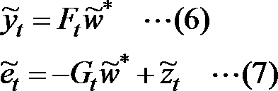
(ただし、*は複素共役)
《従来のビームフォーミングの最適化問題》
まず、従来のビームフォーミングの最適化問題を、確率モデルの観点から定義されたコスト関数の最小化問題として記述する。
まず、従来のビームフォーミングの最適化問題を、確率モデルの観点から定義されたコスト関数の最小化問題として記述する。
~y, ~e, ~w*が確率変数であると解釈し、これらの確率分布Py(~y), Pe(~e), Pw(~w*)は既に分かっているものと仮定する。このうち、確率分布Py(~y), Pe(~e)については、音の統計的な性質が反映されているものと期待される。一方、確率分布Pw(~w*)は、目的音源方角に対する周波数応答の仮定を表現するためにしばしば用いられるものである。これらの仮定のもと、観測音の時系列{~zt}t=1
Tに対する確率変数~w*の尤度関数は

と表される。ただし、~yt, ~etは式(6)、式(7)で表される~w*のアフィン変換によって定まる。この尤度を~w*に関して最大化することで、確率モデルの意味で最適なフィルタが導出できる。尤度最大化は負の対数尤度最小化と等価であるので、解くべきは

という形式の問題になる。
様々な従来のビームフォーミングの最適化問題が式(9)に基づく定式化として解釈できる。以下では、具体例として非特許文献1のMVDRビームフォーマの最適化問題について説明する。
[フィルタ設計フェーズ:フィルタ係数~w*のコスト関数]
周波数ビンfで観測音zfの空間相関行列の推定値Rf=Ez_f[zfzf H](f=1, …, F)が既知であり、また観測音に含まれる推定非目的音~etが正規分布N(0, Rf)に従う(つまり、ef,t~N(0, Rf))と仮定する。
周波数ビンfで観測音zfの空間相関行列の推定値Rf=Ez_f[zfzf H](f=1, …, F)が既知であり、また観測音に含まれる推定非目的音~etが正規分布N(0, Rf)に従う(つまり、ef,t~N(0, Rf))と仮定する。
このとき、尤度関数の非目的音に対する項ΠtPe(~et; ~w*)は
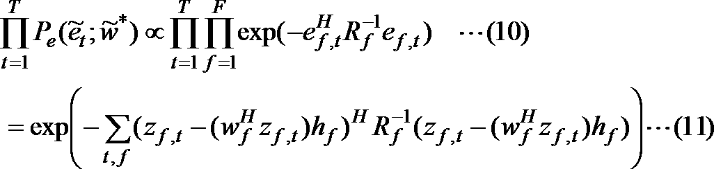
と表される。他の項(ΠtPy(~yt; ~w*)やPw(~w*))にはここでは特に確率分布の仮定をおかない。
[フィルタ設計フェーズ:フィルタ係数~w*の制約条件]
フィルタ係数~w*=(w1 *T, …, wF *T)の各wf *には目的音源方角に対する無歪み制約wf Hhf=1を課す。
フィルタ係数~w*=(w1 *T, …, wF *T)の各wf *には目的音源方角に対する無歪み制約wf Hhf=1を課す。
[フィルタ設計フェーズ:最適化問題]
これらの仮定のもと、単純な平方完成によって式(9)に基づく最適化問題は周波数ビンfについて
これらの仮定のもと、単純な平方完成によって式(9)に基づく最適化問題は周波数ビンfについて

(ただし、γf=(hf
HRf
-1hf)-1)という形に帰着できる。
[フィルタ設計フェーズ:コスト関数最適化]
式(12)の問題の解は、よく知られたMVDRビームフォーマ(すなわち、γfRf -1hf)である。
式(12)の問題の解は、よく知られたMVDRビームフォーマ(すなわち、γfRf -1hf)である。
次に、以上の手続きで得られたフィルタ係数を使用して実際にビームフォーマを動作させる際の計算(フィルタ使用フェーズ)について説明する。
[フィルタ使用フェーズ:フィルタ再設計]
ビームフォーミングの処理では、観測音をフレーム毎に区切り、各フレームに対して離散フーリエ変換を行う必要があるが、リアルタイムでビームフォーミングを行う状況ではフレーム長が長いと遅延が大きくなってしまう。そこで、低遅延のフィルタを再設計する。まず、フィルタ設計フェーズで設計したフィルタ係数~w*に対して逆フーリエ変換を行い、フィルタを時間領域の表現に戻すことで、各マイクロホンm(m=1, …, M)のインパルス応答wm[i]を得る。そして、入力として与えられた指定フレーム長Ntapをもとに、各インパルス応答wm[i]のうち最初のNtap/2成分からなるベクトルw'm1[i]と最後のNtap/2成分からなるベクトルw'm2[i]のみを取り出し(つまり、残りの要素はすべて無視し)、長さがNtapに短縮された新たなインパルス応答
ビームフォーミングの処理では、観測音をフレーム毎に区切り、各フレームに対して離散フーリエ変換を行う必要があるが、リアルタイムでビームフォーミングを行う状況ではフレーム長が長いと遅延が大きくなってしまう。そこで、低遅延のフィルタを再設計する。まず、フィルタ設計フェーズで設計したフィルタ係数~w*に対して逆フーリエ変換を行い、フィルタを時間領域の表現に戻すことで、各マイクロホンm(m=1, …, M)のインパルス応答wm[i]を得る。そして、入力として与えられた指定フレーム長Ntapをもとに、各インパルス応答wm[i]のうち最初のNtap/2成分からなるベクトルw'm1[i]と最後のNtap/2成分からなるベクトルw'm2[i]のみを取り出し(つまり、残りの要素はすべて無視し)、長さがNtapに短縮された新たなインパルス応答

を導入する。このインパルス応答w"m[i]を再度離散フーリエ変換することで、要素数がNtapに削減された(再設計された)フィルタ係数~w'*が計算される。
[フィルタ使用フェーズ:離散フーリエ変換(DFT)]
次に、ビームフォーミング処理対象となる観測音を時間方向にNtapサンプルずつ切り出して、切り出した各区間(フレーム)に対して離散フーリエ変換を施し、STFT領域での観測音~zを出力する。
次に、ビームフォーミング処理対象となる観測音を時間方向にNtapサンプルずつ切り出して、切り出した各区間(フレーム)に対して離散フーリエ変換を施し、STFT領域での観測音~zを出力する。
[フィルタ使用フェーズ:畳み込み]
ここでは、STFT領域での観測音~zとフィルタ係数~w'*を入力とし、式(2)のたたみ込みを行い、STFT領域での推定目的音~yを出力する。
ここでは、STFT領域での観測音~zとフィルタ係数~w'*を入力とし、式(2)のたたみ込みを行い、STFT領域での推定目的音~yを出力する。
[フィルタ使用フェーズ:逆離散フーリエ変換(逆DFT)]
最後に、STFT領域での推定目的音~yに逆離散フーリエ変換を施し、ビームフォーミング処理を施した時間領域波形、つまり時系列の推定目的音を得る。
最後に、STFT領域での推定目的音~yに逆離散フーリエ変換を施し、ビームフォーミング処理を施した時間領域波形、つまり時系列の推定目的音を得る。
式(9)は、変数~w*に関する最適化問題という定式化になっており、上述のMVDRビームフォーマのような比較的単純な例に対しては容易に解くことができるが、コスト関数が複雑な式になる場合、同様に最適化を行うのは一般に困難である。このことから、従来の手法は2つの問題点を抱えていることがわかる。一つ目として、これまでの手法では目的音~yや非目的音~eに対して仮定される確率分布が正規分布のように単純なものに限定されてしまいがちであったが、正規分布は必ずしも音源分布の記述として適切ではない点がある。二つ目として、フィルタ係数~w*に対する制約として用いることができるコスト関数も制限されていて、特に多様な確率的仮定を同時に考慮するのは困難である点がある。これまでにもフィルタ係数~w*に対して付加的な制約の導入を検討したものもあったが、一般に多様な確率的仮定を同時に考慮することで構成されるような複雑なコスト関数の最小化は極めて難しい問題であった。特に、低遅延・安定性・高い雑音抑圧性能を同時に達成するようなビームフォーマを構成するのは困難であった。
上記問題を解決するために、式(6)の推定目的音~ytや式(7)の推定雑音~etのような補助変数に対しても確率的仮定をおき、コスト関数を各補助関数に関するコスト項の和として表現することを考える。以下では、この考えに基づくコスト関数の設計方法について説明する。
《複数の特性を考慮したコスト関数に基づく最適化問題》
ビームフォーミングの最適化問題のための、新たなコスト関数は、さまざまな凸関数の項の和として表現する。また、各項の引数は、フィルタ係数~w*や新たに導入される(推定目的音~ytや推定雑音~etのような)フィルタ係数~w*のアフィン変換として定義できる補助変数とする。。これらの要請を満たすコスト関数は、いずれも最適化問題が解きやすい。言い換えれば、これらの要請を満たす範囲内で自由にコスト関数を設計できる。以下、詳しく説明する。
ビームフォーミングの最適化問題のための、新たなコスト関数は、さまざまな凸関数の項の和として表現する。また、各項の引数は、フィルタ係数~w*や新たに導入される(推定目的音~ytや推定雑音~etのような)フィルタ係数~w*のアフィン変換として定義できる補助変数とする。。これらの要請を満たすコスト関数は、いずれも最適化問題が解きやすい。言い換えれば、これらの要請を満たす範囲内で自由にコスト関数を設計できる。以下、詳しく説明する。
[フィルタ設計フェーズ:フィルタ係数~w*の補助変数]
Jを任意の自然数とし、補助変数vj(j=1, …, J)を導入する。補助変数vjとしてはフィルタ係数~w*と線形の関係、つまり、線形関係式vj=Dj~w*+bjを満たすものを用いる。各補助変数vjとそれがみたす関係式は式(6)、式(7)の一般化になっており、この意味で線形関係式を満たすとの制約は従来の手法を包含するものである。
Jを任意の自然数とし、補助変数vj(j=1, …, J)を導入する。補助変数vjとしてはフィルタ係数~w*と線形の関係、つまり、線形関係式vj=Dj~w*+bjを満たすものを用いる。各補助変数vjとそれがみたす関係式は式(6)、式(7)の一般化になっており、この意味で線形関係式を満たすとの制約は従来の手法を包含するものである。
簡単のため、^v=(v1
T, …, vJ
T)T, ^D=(D1
T, …, DJ
T)T, ^b=(b1
T, …, bJ
T)Tのような表記を以下では採用する。
[フィルタ設計フェーズ:フィルタ係数~w*のコスト項・補助変数vjのコスト項]
コスト関数Lは、フィルタ係数~w*のコスト項L0と補助変数vjのコスト項Lj(j=1, …, J)を用いて
コスト関数Lは、フィルタ係数~w*のコスト項L0と補助変数vjのコスト項Lj(j=1, …, J)を用いて

(ただし、Lj(j=0, …, J)は凸関数)という形式で表す
凸関数の和は凸関数であるから、コスト関数Lも凸関数となる。補助変数vjのコスト項が凸関数であるという制約は一見突飛かもしれないが、これは実は式(6)の推定目的音~ytや式(7)の推定雑音~etなどの補助変数の確率分布にlog-concaveなものを採用していることに他ならない。ここで、確率分布がlog-concaveであるとはその確率密度関数の対数の-1倍(negative log)が凸関数であるという意味である。正規分布やラプラス分布など音源の確率モデルの記述に一般的に用いられる確率分布の多くもこの性質を満たしている。式(14)のコスト項Ljは補助変数vjの確率密度関数の対数の-1倍と解釈できるため、コスト項の凸性はlog-concaveな確率分布のみを考える限り自動的に満たされる性質である。
[フィルタ設計フェーズ:最適化問題]
以上の検討から、我々が解くべき問題は
以上の検討から、我々が解くべき問題は

という典型的な線形制約付き凸最適化問題に帰着できる。式(15)の問題は、フィルタ係数に関する項と補助変数に関する項に分割し、それぞれについて交互に最適化を行うことで解くことができる。この問題を解く具体的なアルゴリズムとして様々なものが知られており、一例として交互方向乗数法(ADMM)を採用したアルゴリズムがある(当該アルゴリズムについて後述する)。
続いて、式(15)の問題定式化において、補助変数に課す確率的仮定として多様なものが使用可能であることを示すため、高い雑音抑圧性能を保ちつつ低遅延かつ音声の強調に適したフィルタを設計する例について説明する。
《複数の特性を考慮したビームフォーマの具体的設計例》
ここでは問題設定として実践的な状況を仮定し、式(15)の枠組みでコスト関数を具体的に設計する例を示す。具体的には、複数の妨害音が鳴っている環境下で、既知の位置から発せられた音声をストリーミング配信する、という状況を仮定する。なお、妨害音源は周波数ビン毎に複素正規分布に従う雑音を発しているものとする。本状況では、目的音源が音声であるという情報を反映した上で、遅延が少なくかつ高い強調性能を保つようなビームフォーマが要望されるだろう。
ここでは問題設定として実践的な状況を仮定し、式(15)の枠組みでコスト関数を具体的に設計する例を示す。具体的には、複数の妨害音が鳴っている環境下で、既知の位置から発せられた音声をストリーミング配信する、という状況を仮定する。なお、妨害音源は周波数ビン毎に複素正規分布に従う雑音を発しているものとする。本状況では、目的音源が音声であるという情報を反映した上で、遅延が少なくかつ高い強調性能を保つようなビームフォーマが要望されるだろう。
[フィルタ設計フェーズ:フィルタ係数~w*のコスト項]
上記状況では特にフィルタ係数~w*におくべき制約は存在しないので、フィルタ係数~w*に対するコスト項L0は考えないことにする。つまり、L0(~w*)=0とする。
上記状況では特にフィルタ係数~w*におくべき制約は存在しないので、フィルタ係数~w*に対するコスト項L0は考えないことにする。つまり、L0(~w*)=0とする。
[フィルタ設計フェーズ:フィルタ係数~w*の補助変数、補助変数のコスト項]
続いて、音源に関して既知の情報やビームフォーマに要望する特性の一つ一つについて検討し、補助変数とそのコスト項の設計を行っていく。
続いて、音源に関して既知の情報やビームフォーマに要望する特性の一つ一つについて検討し、補助変数とそのコスト項の設計を行っていく。
まず、目的音の分布を考える。上記仮定した状況では目的音は音声であるという情報が既知である。音声はスパース性という性質を持つことが知られているため、推定目的音がスパースな確率分布に従うという仮定を考慮したコスト項を設計することで、この既知の情報が活かせると考えられる。そこで、補助変数として推定目的音~ytを採用する。補助変数~ytの定義は式(6)と同一である。そして、補助変数~ytが、次式のラプラス分布に従うという仮定をおく。

ここでβ(>0)は分布の形状を定める定数パラメータである。ラプラス分布はスパースな変数の分布の表現にしばしば用いられるものであり、上記仮定した状況では適切であると考えられる。式(16)の仮定のもと、補助変数~yのコスト項Lyはラプラス分布の対数の-1倍である
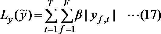
という形になる。ラプラス分布はlog-concaveであるので、コスト項Lyは凸関数になり、式(15)の枠組みのもとで扱える。
次に、非目的音に関しても何らかの確率分布を仮定し、同様に補助変数・コスト項の導入を行う。観測音に含まれる非目的音の推定量として、式(7)で定義される推定非目的音~etを補助変数として導入する。上記仮定した状況では、主に妨害音からなる非目的音は正規分布に従うと仮定する。つまり、補助変数~etは

という確率分布に従って出力されるとみなす。ここで、Rfは非目的音に関する空間相関行列であり、観測データから見積もることができる。式(18)の仮定を、補助変数~eに対するコスト項の形式に書き換えると、

という形になる。正規分布はlog-concaveであるので、このコスト項Leも凸関数である。
ここで更なる補助変数とコスト項を導入することで、ビームフォーマに低遅延性を持たせることを目指す。そのためフィルタ係数~w*にどのようなコスト項を課せば低遅延なフィルタが実現可能か検討する。従来の広帯域ビームフォーマは周波数ビン毎に独立してフィルタ係数を導出しており、隣接周波数ビン間の関連性は考慮していなかった。しかし、周波数ビン方向に不連続やなめらかでないという周波数特性は、時間領域において裾の長いインパルス応答の原因となる。また、位相遅れを引き起こす群遅延も抑制されることが望ましい。このような特性を持たないフィルタ係数を解として得るために、フィルタ係数の周波数ビン方向に関する差分を新たな補助変数として導入し、これらの補助変数(のノルム)を小さくするようなコスト項を課すのが有効であると考えられる。具体的には、新たに

というF-2個の補助変数ηfを定義する。式(20)は、ηfがフィルタの振幅・位相特性の周波数方向に関する2階微分の情報を含むように意図されている。式(20)を用いて、補助変数ηfに対するコスト項Lη_f(ηf)を

で定義する。
[フィルタ設計フェーズ:コスト関数最適化]
以上のように、式(18)、式(16)、式(20)のような補助変数に関する仮定をおいたことで、コスト関数Lは、各コスト項の和
以上のように、式(18)、式(16)、式(20)のような補助変数に関する仮定をおいたことで、コスト関数Lは、各コスト項の和

となる。このコスト関数Lに出現する2FT+F-2個の補助変数はみなフィルタ係数~w*のアフィン変換として表されるので、式(22)の最小化問題は式(15)の具体例である。
ここまではビームフォーミングを対象として最適化問題の議論をしてきたが、これまで説明した数理的な枠組みはより汎用的な適用範囲を持つものであり、音響処理に限られるものではない。本枠組みの汎用性を端的に示すため、上記枠組みを画像処理に適用した例について説明する。
《画像処理における最適化問題の一例》
例えば、同じ形状の物体が大量に写っている画像のように周期的な絵柄の画像(以下、元の画像という)にノイズが重畳された画像が入力として与えられ、当該画像からノイズを除去した画像を得たいという状況を考える。元の画像の各画素の値を表す行列をS=[Sx,y]1≦x≦X,1≦y≦Y、各画素に加わるノイズを表す行列をNと表す。ノイズの値は画素毎に独立に平均0・分散1の正規分布に従って生成されるものとする。我々が観測できるのはノイズを含んだ画像Y=S+Nである。このとき、画像Yから元の画像Sを精度よく推定する問題を考えるため、行列Sを式(15)における~w*とみなし、行列Sや行列Sのアフィン変換によって定まる補助変数に関するコスト項を構成していく。
例えば、同じ形状の物体が大量に写っている画像のように周期的な絵柄の画像(以下、元の画像という)にノイズが重畳された画像が入力として与えられ、当該画像からノイズを除去した画像を得たいという状況を考える。元の画像の各画素の値を表す行列をS=[Sx,y]1≦x≦X,1≦y≦Y、各画素に加わるノイズを表す行列をNと表す。ノイズの値は画素毎に独立に平均0・分散1の正規分布に従って生成されるものとする。我々が観測できるのはノイズを含んだ画像Y=S+Nである。このとき、画像Yから元の画像Sを精度よく推定する問題を考えるため、行列Sを式(15)における~w*とみなし、行列Sや行列Sのアフィン変換によって定まる補助変数に関するコスト項を構成していく。
[フィルタ設計フェーズ:行列Sのコスト項]
まず、推定結果として得られた画像は元の画像と概ね一致していてほしいので、行列Sに関するコスト項として、入力画像Yの各画素との二乗誤差を課すことにする。行列Sに関するコスト項を具体的に書くと、次式になる。
まず、推定結果として得られた画像は元の画像と概ね一致していてほしいので、行列Sに関するコスト項として、入力画像Yの各画素との二乗誤差を課すことにする。行列Sに関するコスト項を具体的に書くと、次式になる。

式(24)のコスト項Lsは凸関数である。
[フィルタ設計フェーズ:補助変数・補助変数のコスト項]
次に、適切にノイズを除去するための補助変数とそのコスト項を設計する。画像は通常滑らかで、隣接画素間の値の変動は小さいということを我々は経験的に知っている。画素毎に独立なノイズはこの性質に反した不自然な振る舞いを示すため、この不自然さを嫌うようなコスト項を設計することでノイズが除去できると考えられる。そこで、隣接画素間の差分として定義される量D1, D2を次式で与えられる補助変数として導入する。
次に、適切にノイズを除去するための補助変数とそのコスト項を設計する。画像は通常滑らかで、隣接画素間の値の変動は小さいということを我々は経験的に知っている。画素毎に独立なノイズはこの性質に反した不自然な振る舞いを示すため、この不自然さを嫌うようなコスト項を設計することでノイズが除去できると考えられる。そこで、隣接画素間の差分として定義される量D1, D2を次式で与えられる補助変数として導入する。

そして、滑らかでより自然性の高い画像ならば補助変数D1, D2の絶対値は傾向として小さくなるはずである。そこで、補助変数D1, D2に対して次のような凸なコスト項を課す。

これらのコスト項LD1, LD2は、ノイズ除去の意味合いを持つコスト項である。
ここでは更に、元の画像が周期的な構造を有するという事前知識を持っている状況を仮定し、このような事前知識を活かせる補助変数やコスト項を設計する。周期的な画像では、画像を2次元フーリエ変換して得られた空間周波数スペクトルがスパースな構造を持つと期待される。2次元フーリエ変換はアフィン変換として記述できるので、空間周波数スペクトルを補助変数として採用することにし、これらの補助変数をスパースに誘導するようなコスト項を設計すれば我々の目的が達成されると考えられる。具体的には、画像の2次元フーリエ変換R=[Rk,j]を補助変数として導入する。これらは離散フーリエ変換行列Wk,jによって

という式で定義でき、確かに行列Sのアフィン変換になっている。コスト項としては、
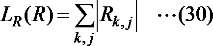
という形の凸関数を仮定する。
[フィルタ設計フェーズ:コスト関数最適化]
以上のコスト項の設計により、最適化すべきコスト関数Lは
以上のコスト項の設計により、最適化すべきコスト関数Lは

という形になる。式(31)の変数のうち行列Sが推定対象の変数であり、その他の変数は行列Sの補助変数である。
以上の議論から、画像処理の場合においても式(15)の枠組みでコスト関数が設計できることがわかる。
《ADMMに基づく最適化アルゴリズム》
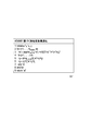
図1は、式(15)で表される線形制約付き凸最適化問題を実際に解くための反復アルゴリズムを示す図である。当該アルゴリズムは式(15)の問題を効率的に解くアルゴリズムの一つとして知られるADMMに基づくものである。ADMMは元の問題の双対問題に対して最適化を行うようなアルゴリズムであり、補助変数vjと同じ次元を持つ双対変数ujを用いる。
図1は、式(15)で表される線形制約付き凸最適化問題を実際に解くための反復アルゴリズムを示す図である。当該アルゴリズムは式(15)の問題を効率的に解くアルゴリズムの一つとして知られるADMMに基づくものである。ADMMは元の問題の双対問題に対して最適化を行うようなアルゴリズムであり、補助変数vjと同じ次元を持つ双対変数ujを用いる。
以下では、ビームフォーマの事例の一つの例として構成したコスト関数(22)に対して図1のアルゴリズムを適用した例について説明する。ここでは、図1の式より具体的な反復更新式を導出する。
まず、変数~w*の更新則に関してはコスト項L0が式(22)では消えていることから、図1のステップ3の式は

という形式に帰着される。この式に現れる行列^DH^D=ΣjDj
HDjは

という形式のブロック帯行列となるため、行列^DH^Dのコレスキー分解を行うことにより更新の際必要になる(^DH^D)-1による乗算の計算を効率化できる。
続いて、補助変数の更新則を求める。この更新則は各コスト項の近接作用素として記述される。ここで、関数fの近接作用素proxfはproxf(x)=argminyf(y)+||x-y||2
2/2という形で定義される。この形とコスト項を見比べると、補助変数yf,tと補助変数ηfの更新則はl2ノルムの近接作用素

で表されることがわかる。一方、補助変数ef,tに関するコスト項は単純な二次形式であるので、ef,tの更新式は定義から解析的に容易に導ける。結局、補助変数の更新則は
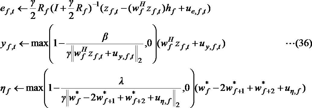
という形になる。ここで、Iは単位行列を表す。
《効果》
本発明の実施形態の原理は、ビームフォーマのフィルタ係数導出をコスト関数最適化問題として解釈した上で、フィルタ係数やその補助変数に対して個別のコスト項に基づく制約を課すことで、所望する複数の特性を兼ね備えたビームフォーマを設計するものである。
本発明の実施形態の原理は、ビームフォーマのフィルタ係数導出をコスト関数最適化問題として解釈した上で、フィルタ係数やその補助変数に対して個別のコスト項に基づく制約を課すことで、所望する複数の特性を兼ね備えたビームフォーマを設計するものである。
従来法では、事前知識や所望する特性などの様々な要因を考慮した複雑なコスト関数を使用した設計を行うことができなかった。一方、本発明の実施形態の原理に従えば、補助変数という形で新たな変数を複数導入し、これらに関して個別にコスト項を設計するという枠組みでコスト関数を構成する。各コスト項は確率的仮定であるという意味を持っており、特にlog-concaveな確率的仮定を課す場合、線形制約付き凸最適化問題に帰着され、様々な数理的手法で比較的容易に最適化問題を解くことができる。これにより、複数の仮定を同時に考慮したフィルタ設計が可能となる。
<第1実施形態>
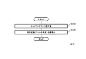
以下、図2~図3を参照して潜在変数最適化装置100を説明する。図2は、潜在変数最適化装置100の構成を示すブロック図である。図3は、潜在変数最適化装置100の動作を示すフローチャートである。図2に示すように潜在変数最適化装置100は、セットアップデータ計算部110と、最適化部120と、記録部190を含む。記録部190は、潜在変数最適化装置100の処理に必要な情報を適宜記録する構成部である。記録部190は、例えば、最適化対象となる潜在変数を記録する。
以下、図2~図3を参照して潜在変数最適化装置100を説明する。図2は、潜在変数最適化装置100の構成を示すブロック図である。図3は、潜在変数最適化装置100の動作を示すフローチャートである。図2に示すように潜在変数最適化装置100は、セットアップデータ計算部110と、最適化部120と、記録部190を含む。記録部190は、潜在変数最適化装置100の処理に必要な情報を適宜記録する構成部である。記録部190は、例えば、最適化対象となる潜在変数を記録する。
潜在変数最適化装置100は、最適化用データを用いて、最適化の対象となるモデルの潜在変数~w*を最適化する。ここで、モデルとは、入力データを入力とし、出力データを出力とする関数(例えば、観測音を入力データとし、目的音を出力データとするビームフォーマのフィルタ)のことであり、最適化用データとは、潜在変数の最適化に用いる入力データ、または、潜在変数の最適化に用いる入力データと出力データの組のことをいう。
図3に従い潜在変数最適化装置100の動作について説明する。
S110において、セットアップデータ計算部110は、最適化用データを用いて、潜在変数~w*を最適化する際に用いるセットアップデータを計算する。例えば、潜在変数~w*を最適化するために用いるコスト関数L

(ただし、vj(1≦j≦J)は行列Djとベクトルbjを用いてvj=Dj~w*+bjと表される潜在変数~w*の補助変数、L0は潜在変数~w*のコスト項、Lj(1≦j≦J)は補助変数vjのコスト項)で用いるDj(1≦j≦J)、bj(1≦j≦J)、コスト項Li(0≦i≦J)に含まれるパラメータがセットアップデータの一例である。なお、コスト項Li(0≦i≦J)は凸関数とするのが好ましい。
例えば、補助変数vj(1≦j≦J)のコスト項は、log-concaveである補助変数vjの確率分布を用いて表されるものとすると、コスト項Li(1≦i≦J)は凸関数となる。また、例えば、潜在変数~w*のコスト項L0=0としてもよく、コスト関数Lは補助変数vj(1≦j≦J)のコスト項の和を含むものであればよい。
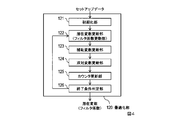
S120において、最適化部120は、コスト関数Lの最小化問題を解くことにより潜在変数~w*を最適化する。以下、図4~図5を参照して最適化部120について説明する。図4は、最適化部120の構成を示すブロック図である。図5は、最適化部120の動作を示すフローチャートである。図4に示すように最適化部120は、初期化部121、潜在変数更新部122と、補助変数更新部123と、双対変数更新部124と、カウンタ更新部125と、終了条件判定部126を含む。
図5に従い最適化部120の動作について説明する。
S121において、初期化部121は、カウンタnを初期化する。具体的には、n=1とする。また、初期化部121は、補助変数^v=(v1
T, …, vJ
T)T、双対変数^u=(u1
T, …, uJ
T)Tを初期化する。さらに、初期化部121は、γにも初期値となる定数を設定する。
S122において、潜在変数更新部122は、現時点で得られている補助変数^v、双対変数^uの値を用いて、次式により、潜在変数~w*を更新する。

ここで、^D=(D1
T, …, DJ
T)T、^b=(b1
T, …, bJ
T)Tである。
S123において、補助変数更新部123は、現時点で得られている潜在変数~w*、双対変数ujの値を用いて、次式により、補助変数vj(1≦j≦J)を更新する。

S124において、双対変数更新部124は、現時点で得られている潜在変数~w*、補助変数vj、双対変数ujの値を用いて、次式により、双対変数uj(1≦j≦J)を更新する。

S125において、カウンタ更新部125は、カウンタnを1だけインクリメントする。具体的には、n←n+1とする。
S126において、終了条件判定部126は、カウンタnが所定の更新回数Niteration(Niterationは1以上の整数であり、例えば10万)に達した場合(つまり、n>Niterationとなり、終了条件が満たされた場合)は、そのときの潜在変数の値~w*を出力して、処理を終了する。それ以外の場合、S122の処理に戻る。つまり、最適化部120は、S122~S126の処理を繰り返す。
なお、式(*)で定義されるコスト関数Lを用いる場合、Jが2以上であっても最適化することができる。
また、式(*)のように、コスト関数Lは、補助変数vjのコスト項をlog-concaveである補助変数vjの確率分布を用いて表されるものとして、補助変数vjのコスト項の和を含むものであればよく、例えば、コスト関数Lは、補助変数vjのコスト項をlog-concaveである補助変数vjの確率分布を用いて表されるものとして、補助変数vjのコスト項とlog-concaveな確率分布に基づいて定まるコスト項との和として表されるものであってもよい。
本実施形態の発明によれば、潜在変数及び潜在変数から定まる補助変数に対する確率的仮定に基づくコスト関数を用いて潜在変数を最適化することが可能となる。
[適用例]
ここでは、潜在変数最適化装置100を音源強調に用いるビームフォーマのフィルタ係数の最適化に適用した例について説明する。そこで、以下では潜在変数最適化装置100のことをフィルタ係数最適化装置100と呼ぶことにする。フィルタ係数最適化装置100の最適化対象はビームフォーマのフィルタ係数となる。フィルタ係数最適化装置100の構成は図2に示す通りである。
ここでは、潜在変数最適化装置100を音源強調に用いるビームフォーマのフィルタ係数の最適化に適用した例について説明する。そこで、以下では潜在変数最適化装置100のことをフィルタ係数最適化装置100と呼ぶことにする。フィルタ係数最適化装置100の最適化対象はビームフォーマのフィルタ係数となる。フィルタ係数最適化装置100の構成は図2に示す通りである。
以下、図3に従いフィルタ係数最適化装置100の動作について説明する。
S110において、セットアップデータ計算部110は、最適化用データを用いて、フィルタ係数~w*=(w1
*T, …, wF
*T)(ただし、wf
*(1≦f≦F)は周波数ビンfのフィルタ係数)を最適化する際に用いるセットアップデータを計算する。例えば、フィルタ係数~w*を最適化するために用いるコスト関数L

(ただし、ef,t(1≦f≦F, 1≦t≦T)は時間フレームtにおける周波数ビンfの推定非目的音を表すフィルタ係数~w*の補助変数、yf,t(1≦f≦F, 1≦t≦T)は時間フレームtにおける周波数ビンfの推定目的音を表すフィルタ係数~w*の補助変数、ηf(1≦f≦F-2)はηf=wf
*-2wf+1
*+wf+2
*で定義されるフィルタ係数~w*の補助変数、Rf(1≦f≦F)は周波数ビンfの非目的音に関する空間相関行列、β(>0)は所定の定数、λは所定の定数)で用いるコスト項Le,f,t(ef,t)=ef,t
HRf
-1ef,t(1≦f≦F, 1≦t≦T)、コスト項Ly,f,t(yf,t)=β|yf,t| (1≦f≦F, 1≦t≦T)、コスト項Lη,f(ηf)=λ||ηf||2(1≦f≦F-2)に含まれるパラメータがセットアップデータの一例である。なお、コスト項Le,f,t(ef,t) (1≦f≦F, 1≦t≦T), Ly,f,t(yf,t) (1≦f≦F, 1≦t≦T)、Lη,f(ηf) (1≦f≦F-2)はいずれも凸関数である。
ただし、コスト項Le,f,t(ef,t), Ly,f,t(yf,t), Lη,f(ηf)は上記コスト項に限るものではなく、例えば、補助変数ef,t, yf,t, ηfのコスト項は、それぞれlog-concaveである補助変数ef,t, yf,t, ηfの確率分布を用いて表されるものであればよい。
なお、上記コスト関数Lの定義式では、フィルタ係数~w*のコスト項L0=0となっている。
S120において、最適化部120は、コスト関数Lの最小化問題を解くことによりフィルタ係数~w*を最適化する。以下、図4~図5を参照して最適化部120について説明する。図4は、最適化部120の構成を示すブロック図である。図5は、最適化部120の動作を示すフローチャートである。ここでは、最適化部120に含まれる潜在変数更新部122のことをフィルタ係数更新部122と呼ぶことにする。
以下、図5に従い最適化部120の動作について説明する。
S121において、初期化部121は、カウンタnを初期化する。具体的には、n=1とする。また、初期化部121は、補助変数^v=[e1,1, …, eF,T, y1,1, …, yF,T, η1, …, ηF-2]、双対変数^u=[ue,1,1, …, ue,F,T, uy,1,1, …, uy,F,T, uη,1, …, uη,F-2](ただし、ue,f,t(1≦f≦F, 1≦t≦T)は補助変数ef,tの双対変数、uy,f,t(1≦f≦F, 1≦t≦T)は補助変数yf,tの双対変数、uη,f(1≦f≦F-2)は補助変数ηfの双対変数とする)を初期化する。さらに、初期化部121は、γにも初期値となる定数を設定する。
S122において、フィルタ係数更新部122は、現時点で得られている補助変数^v、双対変数^uの値を用いて、次式により、フィルタ係数~w*を更新する。

ここで、^D, ^bは次式により与えられる。

S123において、補助変数更新部123は、現時点で得られている潜在変数~w*、双対変数ue,f,t, uy,f,t, uη,fの値を用いて、次式により、補助変数ef,t(1≦f≦F, 1≦t≦T)、補助変数yf,t(1≦f≦F, 1≦t≦T)、補助変数ηf(1≦f≦F-2)を更新する。

(ただし、zf,t(1≦f≦F, 1≦t≦T)は時間フレームtにおける周波数ビンfの観測音、hf(1≦f≦F)は周波数ビンfにおけるビーム方向のアレイマニフォールドベクトル)
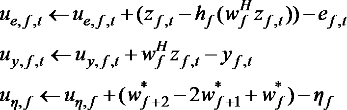
S124において、双対変数更新部124は、現時点で得られている潜在変数~w*、補助変数ef,t, yf,t, ηfの値を用いて、次式により、双対変数ue,f,t, uy,f,t, uη,fを更新する。

S125において、カウンタ更新部125は、カウンタnを1だけインクリメントする。具体的には、n←n+1とする。
S126において、終了条件判定部126は、カウンタnが所定の更新回数Niteration(Niterationは1以上の整数であり、例えば10万)に達した場合(つまり、n>Niterationとなり、終了条件が満たされた場合)は、そのときのフィルタ係数の値~w*を出力して、処理を終了する。それ以外の場合、S122の処理に戻る。つまり、最適化部120は、S122~S126の処理を繰り返す。
なお、式(**)のように、コスト関数Lは、補助変数ef,t, yf,t, ηfのコスト項をそれぞれlog-concaveである補助変数ef,t, yf,t, ηfの確率分布を用いて表されるものとして、補助変数ef,t, yf,t, ηfのコスト項の和を含むものであればよく、例えば、コスト関数Lは、補助変数ef,t, yf,t, ηfのコスト項をそれぞれlog-concaveである補助変数ef,t, yf,t, ηfの確率分布を用いて表されるものとして、補助変数ef,t, yf,t, ηfのコスト項とlog-concaveな確率分布に基づいて定まるコスト項との和として表されるものであってもよい。
<補記>
本発明の装置は、例えば単一のハードウェアエンティティとして、キーボードなどが接続可能な入力部、液晶ディスプレイなどが接続可能な出力部、ハードウェアエンティティの外部に通信可能な通信装置(例えば通信ケーブル)が接続可能な通信部、CPU(Central Processing Unit、キャッシュメモリやレジスタなどを備えていてもよい)、メモリであるRAMやROM、ハードディスクである外部記憶装置並びにこれらの入力部、出力部、通信部、CPU、RAM、ROM、外部記憶装置の間のデータのやり取りが可能なように接続するバスを有している。また必要に応じて、ハードウェアエンティティに、CD-ROMなどの記録媒体を読み書きできる装置(ドライブ)などを設けることとしてもよい。このようなハードウェア資源を備えた物理的実体としては、汎用コンピュータなどがある。
本発明の装置は、例えば単一のハードウェアエンティティとして、キーボードなどが接続可能な入力部、液晶ディスプレイなどが接続可能な出力部、ハードウェアエンティティの外部に通信可能な通信装置(例えば通信ケーブル)が接続可能な通信部、CPU(Central Processing Unit、キャッシュメモリやレジスタなどを備えていてもよい)、メモリであるRAMやROM、ハードディスクである外部記憶装置並びにこれらの入力部、出力部、通信部、CPU、RAM、ROM、外部記憶装置の間のデータのやり取りが可能なように接続するバスを有している。また必要に応じて、ハードウェアエンティティに、CD-ROMなどの記録媒体を読み書きできる装置(ドライブ)などを設けることとしてもよい。このようなハードウェア資源を備えた物理的実体としては、汎用コンピュータなどがある。
ハードウェアエンティティの外部記憶装置には、上述の機能を実現するために必要となるプログラムおよびこのプログラムの処理において必要となるデータなどが記憶されている(外部記憶装置に限らず、例えばプログラムを読み出し専用記憶装置であるROMに記憶させておくこととしてもよい)。また、これらのプログラムの処理によって得られるデータなどは、RAMや外部記憶装置などに適宜に記憶される。
ハードウェアエンティティでは、外部記憶装置(あるいはROMなど)に記憶された各プログラムとこの各プログラムの処理に必要なデータが必要に応じてメモリに読み込まれて、適宜にCPUで解釈実行・処理される。その結果、CPUが所定の機能(上記、…部、…手段などと表した各構成要件)を実現する。
本発明は上述の実施形態に限定されるものではなく、本発明の趣旨を逸脱しない範囲で適宜変更が可能である。また、上記実施形態において説明した処理は、記載の順に従って時系列に実行されるのみならず、処理を実行する装置の処理能力あるいは必要に応じて並列的にあるいは個別に実行されるとしてもよい。
既述のように、上記実施形態において説明したハードウェアエンティティ(本発明の装置)における処理機能をコンピュータによって実現する場合、ハードウェアエンティティが有すべき機能の処理内容はプログラムによって記述される。そして、このプログラムをコンピュータで実行することにより、上記ハードウェアエンティティにおける処理機能がコンピュータ上で実現される。
この処理内容を記述したプログラムは、コンピュータで読み取り可能な記録媒体に記録しておくことができる。コンピュータで読み取り可能な記録媒体としては、例えば、磁気記録装置、光ディスク、光磁気記録媒体、半導体メモリ等どのようなものでもよい。具体的には、例えば、磁気記録装置として、ハードディスク装置、フレキシブルディスク、磁気テープ等を、光ディスクとして、DVD(Digital Versatile Disc)、DVD-RAM(Random Access Memory)、CD-ROM(Compact Disc Read Only Memory)、CD-R(Recordable)/RW(ReWritable)等を、光磁気記録媒体として、MO(Magneto-Optical disc)等を、半導体メモリとしてEEP-ROM(Electronically Erasable and Programmable-Read Only Memory)等を用いることができる。
また、このプログラムの流通は、例えば、そのプログラムを記録したDVD、CD-ROM等の可搬型記録媒体を販売、譲渡、貸与等することによって行う。さらに、このプログラムをサーバコンピュータの記憶装置に格納しておき、ネットワークを介して、サーバコンピュータから他のコンピュータにそのプログラムを転送することにより、このプログラムを流通させる構成としてもよい。
このようなプログラムを実行するコンピュータは、例えば、まず、可搬型記録媒体に記録されたプログラムもしくはサーバコンピュータから転送されたプログラムを、一旦、自己の記憶装置に格納する。そして、処理の実行時、このコンピュータは、自己の記憶装置に格納されたプログラムを読み取り、読み取ったプログラムに従った処理を実行する。また、このプログラムの別の実行形態として、コンピュータが可搬型記録媒体から直接プログラムを読み取り、そのプログラムに従った処理を実行することとしてもよく、さらに、このコンピュータにサーバコンピュータからプログラムが転送されるたびに、逐次、受け取ったプログラムに従った処理を実行することとしてもよい。また、サーバコンピュータから、このコンピュータへのプログラムの転送は行わず、その実行指示と結果取得のみによって処理機能を実現する、いわゆるASP(Application Service Provider)型のサービスによって、上述の処理を実行する構成としてもよい。なお、本形態におけるプログラムには、電子計算機による処理の用に供する情報であってプログラムに準ずるもの(コンピュータに対する直接の指令ではないがコンピュータの処理を規定する性質を有するデータ等)を含むものとする。
また、この形態では、コンピュータ上で所定のプログラムを実行させることにより、ハードウェアエンティティを構成することとしたが、これらの処理内容の少なくとも一部をハードウェア的に実現することとしてもよい。
上述の本発明の実施形態の記載は、例証と記載の目的で提示されたものである。網羅的であるという意思はなく、開示された厳密な形式に発明を限定する意思もない。変形やバリエーションは上述の教示から可能である。実施形態は、本発明の原理の最も良い例証を提供するために、そして、この分野の当業者が、熟考された実際の使用に適するように本発明を色々な実施形態で、また、色々な変形を付加して利用できるようにするために、選ばれて表現されたものである。すべてのそのような変形やバリエーションは、公正に合法的に公平に与えられる幅にしたがって解釈された添付の請求項によって定められた本発明のスコープ内である。
Claims (13)
- 潜在変数~w*を最適化する最適化部を含む潜在変数最適化装置であって、
vj(1≦j≦J)を行列Djとベクトルbjを用いてvj=Dj~w*+bjと表される潜在変数~w*の補助変数とし、
補助変数vjのコスト項は、log-concaveである補助変数vjの確率分布を用いて表されるものであり、
前記最適化部は、
補助変数vjのコスト項の和を含むコスト関数の最小化問題を解くことにより潜在変数~w*を最適化する
潜在変数最適化装置。 - 請求項1に記載の潜在変数最適化装置であって、
前記コスト関数は

潜在変数最適化装置。 - 請求項2に記載の潜在変数最適化装置であって、
uj(1≦j≦J)を補助変数vjの双対変数、^v=(v1 T, …, vJ T)T, ^D=(D1 T, …, DJ T)T, ^b=(b1 T, …, bJ T)T, ^u=(u1 T, …, uJ T)T、γを所定の定数とし、
前記最適化部は、
次式により、潜在変数~w*を更新する潜在変数更新部と、



- ビームフォーマのフィルタ係数~w*=(w1 *T, …, wF *T)(ただし、wf *(1≦f≦F)は周波数ビンfのフィルタ係数)を最適化する最適化部を含むフィルタ係数最適化装置であって、
ef,t(1≦f≦F, 1≦t≦T)を時間フレームtにおける周波数ビンfの推定非目的音を表すフィルタ係数~w*の補助変数、yf,t(1≦f≦F, 1≦t≦T)を時間フレームtにおける周波数ビンfの推定目的音を表すフィルタ係数~w*の補助変数、ηf(1≦f≦F-2)をηf=wf *-2wf+1 *+wf+2 *で定義されるフィルタ係数~w*の補助変数とし、
補助変数ef,t, yf,t, ηfのコスト項は、それぞれlog-concaveである補助変数ef,t, yf,t,ηfの確率分布を用いて表されるものであり、
前記最適化部は、
補助変数ef,t, yf,t, ηfのコスト項の和を含むコスト関数の最小化問題を解くことによりフィルタ係数~w*を最適化する
フィルタ係数最適化装置。 - 請求項4に記載のフィルタ係数最適化装置であって、
前記コスト関数は
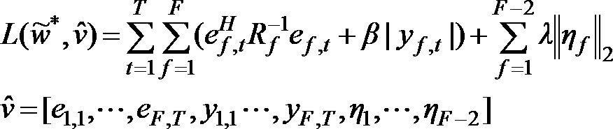
フィルタ係数最適化装置。 - 請求項5に記載のフィルタ係数最適化装置であって、
ue,f,t(1≦f≦F, 1≦t≦T)を補助変数ef,tの双対変数、uy,f,t(1≦f≦F, 1≦t≦T)を補助変数yf,tの双対変数、uη,f(1≦f≦F-2)を補助変数ηfの双対変数、^u=[ue,1,1, …, ue,F,T, uy,1,1, …, uy,F,T, uη,1, …, uη,F-2]、γを所定の定数とし、
前記最適化部は、
次式により、フィルタ係数~w*を更新するフィルタ係数更新部と、

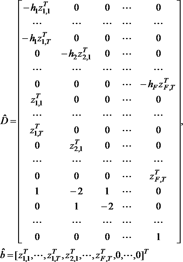
次式により、補助変数ef,t(1≦f≦F, 1≦t≦T)、補助変数yf,t(1≦f≦F, 1≦t≦T)、補助変数ηf(1≦f≦F-2)を更新する補助変数更新部と、

次式により、双対変数ue,f,t(1≦f≦F, 1≦t≦T)、双対変数uy,f,t(1≦f≦F, 1≦t≦T)、双対変数uη,f(1≦f≦F-2)を更新する双対変数更新部と
- ビームフォーマのフィルタ係数~w*=(w1 *T, …, wF *T)(ただし、wf *(1≦f≦F)は周波数ビンfのフィルタ係数)を最適化する最適化部を含むフィルタ係数最適化装置であって、
ηf(1≦f≦F-2)をηf=wf *-2wf+1 *+wf+2 *で定義されるフィルタ係数~w*の補助変数とし、
補助変数ηfのコスト項は、log-concaveである補助変数ηfの確率分布を用いて表されるものであり、
前記最適化部は、
補助変数ηfのコスト項の和を含むコスト関数の最小化問題を解くことによりフィルタ係数~w*を最適化する
フィルタ係数最適化装置。 - 潜在変数最適化装置が、潜在変数~w*を最適化する最適化ステップを実行する潜在変数最適化方法であって、
vj(1≦j≦J)を行列Djとベクトルbjを用いてvj=Dj~w*+bjと表される潜在変数~w*の補助変数とし、
補助変数vjのコスト項は、log-concaveである補助変数vjの確率分布を用いて表されるものであり、
前記最適化ステップは、
補助変数vjのコスト項の和を含むコスト関数の最小化問題を解くことにより潜在変数~w*を最適化する
潜在変数最適化方法。 - 請求項8に記載の潜在変数最適化方法であって、
前記コスト関数は

潜在変数最適化方法。 - フィルタ係数最適化装置が、ビームフォーマのフィルタ係数~w*=(w1 *T, …, wF *T)(ただし、wf *(1≦f≦F)は周波数ビンfのフィルタ係数)を最適化する最適化ステップを実行するフィルタ係数最適化方法であって、
ef,t(1≦f≦F, 1≦t≦T)を時間フレームtにおける周波数ビンfの推定非目的音を表すフィルタ係数~w*の補助変数、yf,t(1≦f≦F, 1≦t≦T)を時間フレームtにおける周波数ビンfの推定目的音を表すフィルタ係数~w*の補助変数、ηf(1≦f≦F-2)をηf=wf *-2wf+1 *+wf+2 *で定義されるフィルタ係数~w*の補助変数とし、
補助変数ef,t, yf,t, ηfのコスト項は、それぞれlog-concaveである補助変数ef,t, yf,t, ηfの確率分布を用いて表されるものであり、
前記最適化ステップは、
補助変数ef,t, yf,t, ηfのコスト項の和を含むコスト関数の最小化問題を解くことによりフィルタ係数~w*を最適化する
フィルタ係数最適化方法。 - 請求項10に記載のフィルタ係数最適化方法であって、
前記コスト関数は

フィルタ係数最適化方法。 - フィルタ係数最適化装置が、ビームフォーマのフィルタ係数~w*=(w1 *T, …, wF *T)(ただし、wf *(1≦f≦F)は周波数ビンfのフィルタ係数)を最適化する最適化ステップを実行するフィルタ係数最適化方法であって、
ηf(1≦f≦F-2)をηf=wf *-2wf+1 *+wf+2 *で定義されるフィルタ係数~w*の補助変数とし、
補助変数ηfのコスト項は、log-concaveである補助変数ηfの確率分布を用いて表されるものであり、
前記最適化ステップは、
補助変数ηfのコスト項の和を含むコスト関数の最小化問題を解くことによりフィルタ係数~w*を最適化する
フィルタ係数最適化方法。 - 請求項1ないし3のいずれか1項に記載の潜在変数最適化装置、請求項4ないし7のいずれか1項に記載のフィルタ係数最適化装置のいずれかとしてコンピュータを機能させるためのプログラム。
Priority Applications (1)
| Application Number | Priority Date | Filing Date | Title |
|---|---|---|---|
| US17/428,251 US20220141584A1 (en) | 2019-02-05 | 2020-01-23 | Latent variable optimization apparatus, filter coefficient optimization apparatus, latent variable optimization method, filter coefficient optimization method, and program |
Applications Claiming Priority (2)
| Application Number | Priority Date | Filing Date | Title |
|---|---|---|---|
| JP2019018424A JP7156064B2 (ja) | 2019-02-05 | 2019-02-05 | 潜在変数最適化装置、フィルタ係数最適化装置、潜在変数最適化方法、フィルタ係数最適化方法、プログラム |
| JP2019-018424 | 2019-02-05 |
Publications (1)
| Publication Number | Publication Date |
|---|---|
| WO2020162188A1 true WO2020162188A1 (ja) | 2020-08-13 |
Family
ID=71948292
Family Applications (1)
| Application Number | Title | Priority Date | Filing Date |
|---|---|---|---|
| PCT/JP2020/002205 Ceased WO2020162188A1 (ja) | 2019-02-05 | 2020-01-23 | 潜在変数最適化装置、フィルタ係数最適化装置、潜在変数最適化方法、フィルタ係数最適化方法、プログラム |
Country Status (3)
| Country | Link |
|---|---|
| US (1) | US20220141584A1 (ja) |
| JP (1) | JP7156064B2 (ja) |
| WO (1) | WO2020162188A1 (ja) |
Families Citing this family (1)
| Publication number | Priority date | Publication date | Assignee | Title |
|---|---|---|---|---|
| JP7375904B2 (ja) * | 2020-02-28 | 2023-11-08 | 日本電信電話株式会社 | フィルタ係数最適化装置、潜在変数最適化装置、フィルタ係数最適化方法、潜在変数最適化方法、プログラム |
Citations (1)
| Publication number | Priority date | Publication date | Assignee | Title |
|---|---|---|---|---|
| US9668066B1 (en) * | 2015-04-03 | 2017-05-30 | Cedar Audio Ltd. | Blind source separation systems |
-
2019
- 2019-02-05 JP JP2019018424A patent/JP7156064B2/ja active Active
-
2020
- 2020-01-23 WO PCT/JP2020/002205 patent/WO2020162188A1/ja not_active Ceased
- 2020-01-23 US US17/428,251 patent/US20220141584A1/en not_active Abandoned
Patent Citations (1)
| Publication number | Priority date | Publication date | Assignee | Title |
|---|---|---|---|---|
| US9668066B1 (en) * | 2015-04-03 | 2017-05-30 | Cedar Audio Ltd. | Blind source separation systems |
Also Published As
| Publication number | Publication date |
|---|---|
| JP2020126138A (ja) | 2020-08-20 |
| US20220141584A1 (en) | 2022-05-05 |
| JP7156064B2 (ja) | 2022-10-19 |
Similar Documents
| Publication | Publication Date | Title |
|---|---|---|
| JP2009037597A (ja) | 入力画像をフィルタリングして出力画像を作成する方法 | |
| US20250308543A1 (en) | Meta-learning for adaptive filters | |
| Cheng et al. | Semi-blind source separation using convolutive transfer function for nonlinear acoustic echo cancellation | |
| Lee et al. | Independent vector analysis based on overlapped cliques of variable width for frequency-domain blind signal separation | |
| Bayram et al. | Primal-dual algorithms for audio decomposition using mixed norms | |
| WO2022172441A1 (ja) | 音源分離装置、音源分離方法、およびプログラム | |
| JP7167746B2 (ja) | 非負値行列分解最適化装置、非負値行列分解最適化方法、プログラム | |
| JP7114497B2 (ja) | 変数最適化装置、変数最適化方法、プログラム | |
| WO2020162188A1 (ja) | 潜在変数最適化装置、フィルタ係数最適化装置、潜在変数最適化方法、フィルタ係数最適化方法、プログラム | |
| WO2021255925A1 (ja) | 目的音信号生成装置、目的音信号生成方法、プログラム | |
| JP7351401B2 (ja) | 信号処理装置、信号処理方法、およびプログラム | |
| Li et al. | Adaptive physics-informed neural networks for underwater acoustic field prediction | |
| Xiaohui et al. | An algorithm of generating random number by wavelet denoising method and its application | |
| JP6290803B2 (ja) | モデル推定装置、目的音強調装置、モデル推定方法及びモデル推定プログラム | |
| JP7159928B2 (ja) | 雑音空間共分散行列推定装置、雑音空間共分散行列推定方法、およびプログラム | |
| JP7709139B2 (ja) | 信号処理装置、信号処理方法、およびプログラム | |
| JP7375904B2 (ja) | フィルタ係数最適化装置、潜在変数最適化装置、フィルタ係数最適化方法、潜在変数最適化方法、プログラム | |
| JP7444243B2 (ja) | 信号処理装置、信号処理方法、およびプログラム | |
| CN109074811B (zh) | 音频源分离 | |
| JP7235129B2 (ja) | 変数最適化装置、変数最適化方法、プログラム | |
| JP7173355B2 (ja) | Psd最適化装置、psd最適化方法、プログラム | |
| JP2020030373A (ja) | 音源強調装置、音源強調学習装置、音源強調方法、プログラム | |
| JP7375905B2 (ja) | フィルタ係数最適化装置、フィルタ係数最適化方法、プログラム | |
| JP7173356B2 (ja) | Psd最適化装置、psd最適化方法、プログラム | |
| WO2021100136A1 (ja) | 音源信号推定装置、音源信号推定方法、プログラム |
Legal Events
| Date | Code | Title | Description |
|---|---|---|---|
| 121 | Ep: the epo has been informed by wipo that ep was designated in this application |
Ref document number: 20752881 Country of ref document: EP Kind code of ref document: A1 |
|
| NENP | Non-entry into the national phase |
Ref country code: DE |
|
| 122 | Ep: pct application non-entry in european phase |
Ref document number: 20752881 Country of ref document: EP Kind code of ref document: A1 |