WO2020158032A1 - 推定装置、学習装置、それらの方法、およびプログラム - Google Patents
推定装置、学習装置、それらの方法、およびプログラム Download PDFInfo
- Publication number
- WO2020158032A1 WO2020158032A1 PCT/JP2019/034216 JP2019034216W WO2020158032A1 WO 2020158032 A1 WO2020158032 A1 WO 2020158032A1 JP 2019034216 W JP2019034216 W JP 2019034216W WO 2020158032 A1 WO2020158032 A1 WO 2020158032A1
- Authority
- WO
- WIPO (PCT)
- Prior art keywords
- state
- parameter
- observation
- amount
- value
- Prior art date
- Legal status (The legal status is an assumption and is not a legal conclusion. Google has not performed a legal analysis and makes no representation as to the accuracy of the status listed.)
- Ceased
Links
Images






Classifications
-
- G—PHYSICS
- G06—COMPUTING OR CALCULATING; COUNTING
- G06N—COMPUTING ARRANGEMENTS BASED ON SPECIFIC COMPUTATIONAL MODELS
- G06N3/00—Computing arrangements based on biological models
- G06N3/02—Neural networks
- G06N3/04—Architecture, e.g. interconnection topology
- G06N3/047—Probabilistic or stochastic networks
-
- G—PHYSICS
- G06—COMPUTING OR CALCULATING; COUNTING
- G06N—COMPUTING ARRANGEMENTS BASED ON SPECIFIC COMPUTATIONAL MODELS
- G06N3/00—Computing arrangements based on biological models
- G06N3/02—Neural networks
- G06N3/04—Architecture, e.g. interconnection topology
- G06N3/045—Combinations of networks
- G06N3/0455—Auto-encoder networks; Encoder-decoder networks
-
- G—PHYSICS
- G06—COMPUTING OR CALCULATING; COUNTING
- G06N—COMPUTING ARRANGEMENTS BASED ON SPECIFIC COMPUTATIONAL MODELS
- G06N3/00—Computing arrangements based on biological models
- G06N3/02—Neural networks
- G06N3/04—Architecture, e.g. interconnection topology
- G06N3/0475—Generative networks
-
- G—PHYSICS
- G06—COMPUTING OR CALCULATING; COUNTING
- G06N—COMPUTING ARRANGEMENTS BASED ON SPECIFIC COMPUTATIONAL MODELS
- G06N3/00—Computing arrangements based on biological models
- G06N3/02—Neural networks
- G06N3/08—Learning methods
- G06N3/084—Backpropagation, e.g. using gradient descent
-
- G—PHYSICS
- G06—COMPUTING OR CALCULATING; COUNTING
- G06N—COMPUTING ARRANGEMENTS BASED ON SPECIFIC COMPUTATIONAL MODELS
- G06N3/00—Computing arrangements based on biological models
- G06N3/02—Neural networks
- G06N3/08—Learning methods
- G06N3/09—Supervised learning
Definitions
- the present invention relates to an estimation device, a learning device, a method thereof, and a program for estimating a state from an observed amount using a state space model.
- a framework called a state space model is widely used to analyze the properties of objects from series data.
- the state space model consists of hidden “state models” that cannot be observed and “observation models” that are the results of observation.
- a quantity called a state evolves over time, and the observed quantities (for example, current and sound pressure) are evolved from these states through the observation process.
- -A model that thinks that "quantity" series data such as images will be generated.
- the state is non-linear and changes over time (time evolution), and the observed amount can be obtained (through the observation process) by performing observation processing that changes non-linearly over time with the time transition of the state. Due to the non-linearity of the observation process and time evolution, it is difficult to learn all state-space models from observables only without prior assumptions. On the other hand, a technique called Koopman mode decomposition, which has been studied in recent years, can avoid the above-mentioned nonlinearity by considering a state space model in another region (function space) (Non-Patent Document 1, 2).
- the present invention provides a learning device that learns an observation process, time evolution, and a state from only an observation amount, an estimation device that estimates a state from an observation amount using an observation process, a time evolution, and a state that is learned only from an observation amount, and
- the purpose is to provide a method and a program.
- an estimation apparatus uses an encoder to estimate an observation amount from a state using a state estimation unit that estimates a state from an observation amount, and a decoder.
- An observing quantity estimating unit for estimating and a future observing quantity estimating unit for estimating a future observing quantity which is a value in which the observing quantity fluctuates with time using the parameter K representing the time expansion, and has an encoder parameter.
- the parameter of the decoder and the parameter K are optimized at the same time.
- the present invention it is possible to learn the observation process/time evolution/state only from the observation amount. Further, it is possible to estimate the state from the observed amount by using the observation process, time evolution, and state learned from only the observed amount.
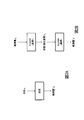
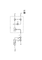
- FIG. 2A is a diagram for explaining a spatial state model of a conventional technique
- FIG. 2B is a diagram for explaining a framework of the auto encoder of the first embodiment.
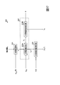
- the functional block diagram of the learning device which concerns on 1st embodiment.
- the functional block diagram of the estimation apparatus which concerns on 1st embodiment.
- the figure for demonstrating the algorithm of an estimation stage The figure which shows the outline
- FIG. 2A is a diagram for explaining a spatial state model of a conventional technique
- FIG. 2B is a diagram for explaining a framework of the auto encoder of the first embodiment.
- the functional block diagram of the abnormality detection apparatus which concerns on 2nd embodiment. The figure which shows the example of the process flow of the pre-process of the abnormality detection apparatus which concerns on 2nd embodiment.
- the functional block diagram of the learning device which concerns on 3rd embodiment.
- the functional block diagram of the estimation part of the estimation apparatus which concerns on 3rd embodiment.
- the present embodiment makes it possible to learn not only the time evolution and the observation process but also the “inverse function” of the observation process at the same time, so that all of the observation process, the time evolution, and the state can be learned from only the observed amount.
- the auto encoder network see Reference 1 is used.
- Reference 1 G. E. Hinton. "Reducing the Dimensionality of Data with Neural Networks", Science, 313(5786):504-507, July 2006.
- Auto-encoder converts a certain input into a low dimension by a network called an encoder and restores it by a network called a decoder.
- the basic technology of the present embodiment is that both of them can be learned at the same time by regarding the encoder as an “inverse function” and the decoder as an observation process.
- the state space model includes an observation model that estimates an observed amount from a state that changes over time and is unobservable, and a state model that estimates a state that changes over time.
- the state space model is premised on estimating the observed amount from the state.
- such a model cannot be constructed when the state is unknown.
- the encoder is used as a model for estimating the state from the observed quantity
- the decoder is By learning as a model for estimating the observed amount, we made it possible to construct a model for estimating the observed amount from the state. In other words, it may be said that the model is constructed so as to learn a model in which input and output are reversed.
- the state may be abstract or concrete.
- the state evolves over time as follows.
- x t+1 f(x t ) (1)
- the observed amount is a value that is digitized by some method (for example, current voltage, temperature, sound pressure, image, etc.), and may be multidimensional data obtained by a microphone array.
- the goal in the framework of the state-space model is to obtain the sequence data ⁇ y 1 ,...,y T ⁇ of observables, ⁇ State series data ⁇ x 1 ,...,x T ⁇ ⁇ Time evolution function f(x t ) ⁇ Function of observation process g(x t ) Is to decide.
- Koopman mode decomposition is a method that can avoid the aforementioned non-linearity. (Koopman mode decomposition) Basis functions
- Koopman mode decomposition can avoid the above non-linearity by discussing it in the function space.
- Koopman mode decomposition is applicable when the state x t is known. Therefore, even if Koopman mode decomposition is used, it is difficult to learn the time evolution, the observation process, and the state only from the series data of the observed amount.
- a new state estimation method is devised based on the framework of Koopman mode decomposition.
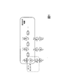
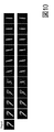
- FIG. 1 shows an outline of this embodiment.
- the state data x t , observation process ( ⁇ ,B), and time evolution K are learned by inputting the observation data series data ⁇ y t ⁇ . After learning, it outputs the sequence data ⁇ y 1 (t) , ⁇ y 2 (t) , ... and the state x t of the observed amount predicted from a certain observed amount y t .
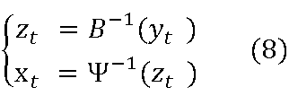
- Is. B -1 (•) can be analytically obtained by pseudo-inverse matrix of B or Ridge regression.
- An auto-encoder network is a neural network used to reduce the dimension of data. An input is transferred to an intermediate layer through an encoder and reconstructed through a decoder. That is,
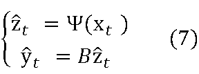
- the encoder ⁇ ⁇ 1 is the inverse function ⁇ ⁇ 1 ( ⁇ ) of the basis function and the decoder ⁇ is the basis function ⁇ ( ⁇ ).
- the state x t is transformed into ⁇ z t on the basis, and the time elapses so as to obtain a spatial state model that derives the observed amount ⁇ y t predicted from ⁇ z t and the coefficient B.
- a base was obtained which was linearly transformed according to (see FIGS. 1 and 2A).
- it is learned using an encoder that outputs enter the observed quantity y t state x t, decoder for outputting enter the state x t observed quantity ⁇ y t, and so as the framework of Autoencoder (See FIGS. 1 and 2B).
- This embodiment is divided into two stages.
- One is a stage (hereinafter also referred to as a learning stage) for learning the time evolution, the observation process, and its inverse function from the time series data of the observed amount.
- One is the stage of acquiring the state from the observed amount (hereinafter also referred to as the state acquisition stage).
- the state acquisition system includes a learning device 100 and a state acquisition device 200 (see FIG. 3). Since the state acquisition device 200 estimates the state from the observed amount or the observed amount from the state, it is also referred to as the estimation device 200. Similarly, the state acquisition stage is also called an estimation stage, and the state acquisition system is also called an estimation system.
- the learning device 100 executes the above-mentioned learning stage, and the estimation device 200 executes the above-mentioned estimation stage. First, the learning stage will be described.
- FIG. 4 shows a functional block diagram of the learning device 100
- FIG. 5 shows an example of its processing flow.
- the learning device 100 includes an initialization unit 110, an estimation unit 120, an objective function calculation unit 130, and a parameter updating unit 140.
- the learning device 100 receives the series data ⁇ y t (L) ⁇ of the observation amount for learning, and outputs the parameters (w enc , w dec , K, B) as the learning result.
- w enc is the parameter used in the encoder (the parameter of the inverse function ⁇ ⁇ 1 )
- w dec is the parameter used in the decoder (the parameter of the basis function ⁇ )
- K is the parameter representing the time evolution
- B is the expansion coefficient. ..
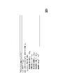
- the learning stage is performed as in Algorithm 1 of FIG.
- An example is shown in which the observation amount for learning is data based on image data.
- the data y t based on the image data may be, for example, data having a pixel value of each pixel and having dimensions corresponding to the number of pixels, or a feature amount obtained from the image data or a feature amount obtained from the moving image data.
- the state represents an abstract state corresponding to the observed amount y t , and this abstract state has a physical meaning (e.g., lower than the observed amount). Dimension value).
- the state represents an amount similar to the size and position of a periodic pattern or object appearing in the image data, or an amount similar to the phase of the moving object in the moving image data including the image data (when periodically operating).
- the estimation unit 120 inputs the observation observation series data ⁇ y t (L) ⁇ and the initialized or updated parameters w enc (k) ,w dec (k) ,K (k) ,B (k) . , (1) Estimating the value of the basis function (estimated value z t ), (2) Estimating the state (estimated value x t ), (3) Estimating the value of the reconstructed basis function (estimated value ⁇ z t ).
- B (k)+ (•) represents solving the regression problem.
- B (k) + ( ⁇ ) (B (k) T B (k) + ⁇ I) -1
- B (k) T ⁇ is a problem in the Ridge regression, using the pseudo-inverse matrix
- a sparse estimation algorithm such as linear regression or LASSO may be used.
- ⁇ is a predetermined weighting parameter in Ridge regression.
- the objective function calculation unit 130 uses the observation observation series data ⁇ y t+ ⁇ (L) ⁇ and the estimated value series data ⁇ z t+ ⁇ ⁇ , ⁇ x t+ ⁇ ⁇ , ⁇ z t+ ⁇ ⁇ , predicted value series data ⁇ z ⁇ (t) ⁇ , ⁇ y ⁇ (t) ⁇ , parameters w enc (k) and w dec (k) are input, and the value of the objective function J( ⁇ ) Is calculated (S130) and output.
- ⁇ is a set of parameters w enc (k) , w dec (k) , K (k) , and B (k) .
- ⁇ ⁇ is 0 ⁇ ⁇ ⁇ 1, and is a weighting parameter for setting so that the error at the time t+ ⁇ closer to the current time t is evaluated larger, and E[ ⁇ ] represents the expected value calculation.
- the updated parameters w enc (k+1) , w dec (k+1) ,K (k+1) ,B (k+1) is provided to the estimation unit 120, and updated parameters w enc (k+1) ,w dec (k+1 ) for calculating the regularization term ⁇ 1 are calculated.
- the parameter update is aborted and the model learning is terminated.
- the latest parameters w enc (k) ,w dec (k) ,K (k) ,B (k) are output to the estimation device 200 as parameters (w enc ,w dec ,K,B) which are learning results. ..
- FIG. 7 shows a functional block diagram of the estimation device 200, and FIG. 8 shows an example of the processing flow thereof.
- the estimation device 200 includes an estimation unit 220.
- estimation device 200 sets the parameters (w enc , w dec , K, B) received from the learning device 100 in the estimation unit 220 prior to the estimation and prediction.
- Algorithm 2 When running the algorithm 2 in FIG. 9, the estimating apparatus 200 inputs the observed quantity y t, estimates the state corresponding to the observed quantity y t, predicting time series data of the observed quantity after y t, the estimated value Output x t , the predicted series data ⁇ y ⁇ (t) ⁇ .
- the estimation unit 220 can predict the image data at the T-step ahead by using the data based on appropriate image data as the observed amount y t .
- observation series data y t ,y t+1 ,...,y t+N and estimating series data x t ,x t+1 ,...,x t+N and predicted N
- the series data ⁇ y ⁇ (t) ⁇ , ⁇ y ⁇ (t+1) ⁇ ,..., ⁇ y ⁇ (t+N) ⁇ may be output.
- the estimation unit 220 receives the observed amount y t as input, and estimates the state by performing a predetermined process on the observed amount y t (S220).
- the predetermined processing is (1) estimation of the value of the basis function (estimated value z t ) and (2) estimation of the state (estimated value x t ).
- the estimation unit 220 includes (3) estimation of the value of the reconstructed basis function (estimated value ⁇ z t ), (4) prediction of the basis function (predicted value ⁇ z ⁇ (t) ), (5) observed amount Is performed (predicted value ⁇ y ⁇ (t) ) (S220), and the estimated value xt and predicted value series data ⁇ y ⁇ (t) ⁇ are output.
- processes (3) to (5) above are processes that obtain the observed amount from the state, and can be said to be the reverse process of the above processes (1) and (2).
- FIG. 10 shows an example of actually generating series data by learning parameters by inputting series data of data based on image data.
- the upper part of FIG. 10 is the series data of the data based on the actual image data (the series data of the observed amount for learning).
- Algorithm 3 When executing the algorithm 3 of FIG. 11, the estimation apparatus 200 receives the state x t as input, predicts the observed amount corresponding to the state x t , and outputs the predicted series data ⁇ y ⁇ (t) ⁇ . In Algorithm 3 of FIG. 11, it is possible to give an appropriate state x t to the estimation unit 220 and predict an image up to T steps ahead.
- the estimation unit 220 receives a certain state x t as input, (1) estimation of the value of the reconstructed basis function (estimated value ⁇ z t ), (2) prediction of the basis function (predicted value ⁇ z ⁇ (t) ). , (3) prediction of the observed amount (predicted value ⁇ y ⁇ (t) ) is performed (S220), and the series data ⁇ y ⁇ (t) ⁇ of the predicted value is output.
- the state can be estimated from the observed amount by using the observation process, time evolution, and state (learned model) learned from only the observed amount.
- the observed quantity can be predicted from the estimated state and the given state. That is, the sequence data can be predicted by estimating the state from the current observed amount, simulating the time evolution, and observing the state. Further, by giving an observation amount and a state, it is possible to artificially generate data (state, observation amount).
- State can be estimated from series data observed by sensors, etc., and can be used for analysis of observed quantities. In addition, it is easy to visually grasp the observed amount by estimating the state (for example, the number of dimensions is small) from the series data that is difficult to visually grasp (for example, the number of dimensions is large) and presenting the estimated state. Can be converted to (visualized).
- ⁇ Modification> the case where the observation amount is data based on image data has been described, but other data may be used.
- data based on acoustic data, data based on vibration data, a combination of data based on acoustic data and data based on vibration data, and the like can be considered. The details will be described below.
- the sound pressure waveform data obtained from the microphone or its characteristic amount STFT, log-Mel power, etc.
- STFT log-Mel power, etc.
- a vector obtained by combining sound pressure waveform data or its characteristic amount by the number of elements is used as the input y t .
- the state represents an abstract state corresponding to the observed amount y t
- this abstract state can be a value having a physical meaning (for example, a value of a lower dimension than the observed amount).
- the state represents an amount similar to the waveform of the sound source, an amount similar to the position of the sound source (when the sound source moves), and an amount similar to the phase (when the sound is periodic).
- the state represents an abstract state corresponding to the observed amount y t
- this abstract state can be a value having a physical meaning (for example, a value of a lower dimension than the observed amount).
- the state represents an amount similar to a mode of vibration, an amount similar to a phase (in the case of vibration of a quasi-periodically moving object), and the like.
- the state x t represents an abstract state corresponding to the observed amount y t
- this abstract state can be a value having a physical meaning (for example, a value of a lower dimension than the observed amount).
- the state represents an amount similar to a waveform of a sound source (vibration source), an amount similar to a vibration mode, and the like.
- the present invention is applied to abnormality detection.
- FIG. 12 shows a functional block diagram of the abnormality detection device according to the present embodiment.
- the learning device 100 learns the parameters (w enc ,w dec ,K,B) by using the observation observation series data ⁇ y t (L) ⁇ for learning as an input. And output.
- the estimation device 200 sets the parameters (w enc , w dec , K, B) received from the learning device 100 in the estimation unit 220 prior to estimation and prediction.
- the abnormality detection device 300 includes an error vector calculation unit 310, an average variance/covariance matrix calculation unit 320, and a detection unit 330 (see FIG. 12 ).
- the abnormality detection device 300 executes an abnormality detection process and a pre-process for obtaining a parameter in advance before the abnormality detection process. First, the preprocessing will be described.
- the subscript A_B means A B.
- Fig. 13 shows an example of the processing flow of preprocessing.
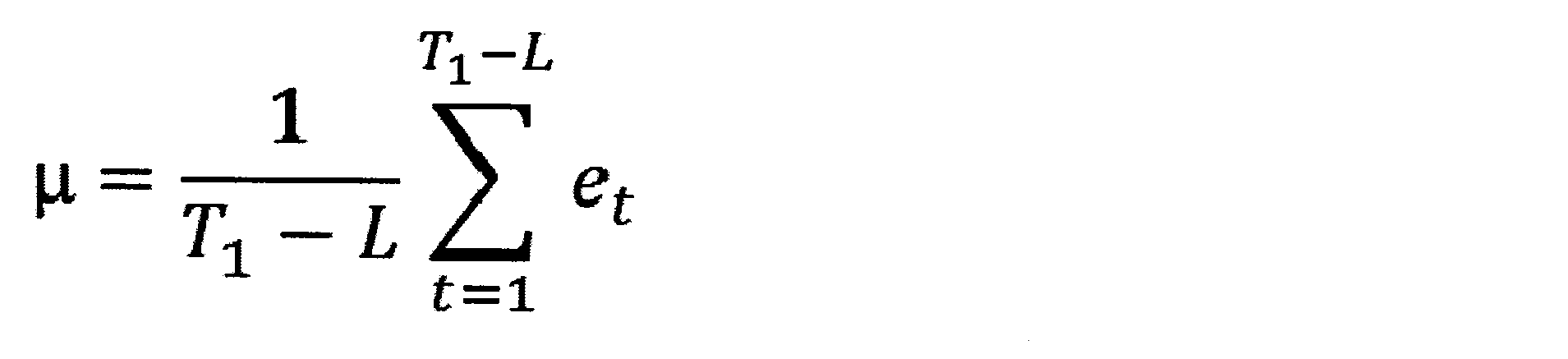
- the anomaly detection apparatus 300 collects T 1 -L partial series D t and T 1 -L predicted series data P t obtained from the data set D normal of the observed amount at the normal time. As an input, a mean ⁇ and a variance-covariance matrix S described later are calculated.
- the error vector e t is a vector of length (D ⁇ L) when the dimension of the observation amount y t is D.
- the above error vector calculation is performed for all T 1 -L subseries D t and series data P t .
- FIG. 14 shows an example of the processing flow of abnormality detection processing.
- the anomaly detection apparatus 300 uses the T 2 -L partial series D' t' and the T 2 -L predicted series data obtained from the data set D new of the observed amount to be anomaly detected.
- P 't' ⁇ y '(t') 1, ..., ⁇ y '(t') L ⁇ as input and outputs a detection result of the partial sequence D 't' and series data P 't' ..
- the detection unit 330 receives the average ⁇ and the variance-covariance matrix S prior to the abnormality detection.
- L t ' logdet (S) + (e' t '- ⁇ ) T S -1 (e' t '- ⁇ ) T
- the abnormality degree L t ′ is an amount proportional to the negative logarithmic likelihood when the error vector is fitted with a normal distribution.
- the detection unit 330 determines whether or not there is an abnormality based on the magnitude relationship between the value corresponding to the abnormality degree L t ′ and the threshold value p, detects the abnormality (S330-2), and outputs the detection result. .. For example, when the degree of abnormality L t′ >p, it is determined to be abnormal, and when L t′ ⁇ p, it is determined not to be abnormal.
- the threshold p is appropriately determined in advance by experiments, simulations, etc.
- the present invention can be applied to abnormality detection.
- the prediction value ⁇ y ⁇ (t) are considering if predicted from the state x t observables of the inverse function to a function for outputting (the prediction value ⁇ y ⁇ (t)) is present.
- the state x t has a lower dimension than the prediction of the observed quantity (predicted value ⁇ y ⁇ (t) )
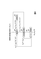
- FIG. 15 shows an extended dynamic mode decomposition (EDMD) part which is a numerical calculation method of Koopman mode decomposition.
- EDMD extended dynamic mode decomposition
- the mean and variance parameters are estimated from the observed quantities y t and y t+1 using a neural network (( ⁇ t , ⁇ t ) ⁇ (y t ,y t+1 )).
- This process corresponds to the encoding of the variational auto encoder, and the part that realizes this process is called an encoder.
- the latent variable (state x t ) is sampled from the multivariate normal distribution according to the obtained mean estimate ⁇ t and variance parameter estimate ⁇ t .
- e t in the figure is a random number obtained from a normal distribution with mean 0 and variance 1.
- a normal variational auto encoder learns the weighting parameter ⁇ of the neural network so as to minimize the following objective function.
- B] represents the Kullback-Leibler divergence of distributions A and B
- N( ⁇ , ⁇ ) represents the distribution of mean ⁇ and variance ⁇
- ⁇ ⁇ (y t ) represents the distribution of mean ⁇ and variance ⁇
- ⁇ ⁇ (y t ) represents the mean and variance parameters estimated by giving the observed amount y t+ ⁇ to the neural network with the weight parameter ⁇ .
- the expansion coefficient B and the parameter K are learned and optimized at the same time as the weighting parameter ⁇ . That is,
- ⁇ y ⁇ (t) BK ⁇ ⁇ z t
- ⁇ ⁇ (y t+ ⁇ ,y t+ ⁇ +1 ) and ⁇ ⁇ (y t+ ⁇ ,y t+ ⁇ +1 ) are respectively Mean and variance parameters estimated by giving the observed quantities y t+ ⁇ and y t+ ⁇ +1 to the neural network of the weight parameter ⁇ are shown. The following two points can be mentioned as the difference between the first embodiment and this embodiment.
- the first embodiment assumed an inverse function, but this embodiment assumes a stochastic generative model.
- the reconstruction error was minimized as an objective function, but in this embodiment, a Kullback-Leibler divergence term that measures the closeness of the distribution is added to the reconstruction error.
- the estimation system includes a learning device 100 and an estimation device 200 (see FIG. 3).
- the learning device 100 executes the learning stage, and the estimation device 200 executes the estimation stage. First, the learning stage will be described.
- FIG. 16 is a functional block diagram of the learning device 100, and FIG. 5 shows an example of the processing flow.
- the learning device 100 includes an initialization unit 110, an estimation unit 120, an objective function calculation unit 130, and a parameter updating unit 140.
- the learning device 100 inputs the series data ⁇ y t ⁇ of the observation amount for learning and outputs the parameters (w enc , w dec , K, B) which are the learning results.
- w enc is a parameter used in the encoder
- w dec is a parameter used in the decoder (parameter of the basis function ⁇ )
- K is a parameter representing time evolution
- B is an expansion coefficient.
- the learning phase is as follows.
- the parameter updating unit 140 receives and processes the objective function L(B (k) , K (k) , ⁇ (k) ) instead of the objective function J( ⁇ (k) ).
- the estimation unit 120 receives as input the observation observation series data ⁇ y t ⁇ and the initialized or updated parameters w enc (k) ,w dec (k) ,K (k) ,B (k). 1) State mean and variance parameter estimation (estimated values ⁇ t , ⁇ t ), (2) State estimation (estimated value x t ), (3) Reconstructed basis function value estimation (estimated value ⁇ z t ), (4) Basis function prediction (predicted value ⁇ z ⁇ (t) ), (5) Observed amount prediction (predicted value ⁇ y ⁇ (t) ) (S120), predicted value ⁇ y ⁇ ( output t) . Since (3) to (5) are the same as those in the first embodiment, (1) and (2) will be described.
- the objective function calculation unit 130 receives the learning observation series data ⁇ y t+ ⁇ ⁇ , the predicted value series data ⁇ y ⁇ (t) ⁇ , and the parameter w enc (k) as input, The value L(B (k) , K (k) , ⁇ (k) ) is calculated (S130) and output. Note that ⁇ (k) is a set of parameters w enc (k) and w dec (k) .
- ⁇ y ⁇ (t) B (k) K (k) ⁇ ⁇ z t .
- y ⁇ and y ⁇ +1 are required to update K (k) at the same time, and ⁇ is any integer of 1 or more.
- c and d are parameters for deciding how much importance is attached to each term, and are set appropriately by using experimental results, simulation results, and the like.
- FIG. 7 shows a functional block diagram of the estimation device 200, and FIG. 8 shows an example of the processing flow thereof.
- the estimation device 200 includes an estimation unit 220.
- estimation device 200 sets the parameters (w enc , w dec , K, B) received from the learning device 100 in the estimation unit 220 prior to the estimation and prediction.
- observation series data y t ,y t+1 ,...,y t+N and estimating series data x t ,x t+1 ,...,x t+N and predicted N
- the series data ⁇ y ⁇ (t) ⁇ , ⁇ y ⁇ (t+1) ⁇ ,..., ⁇ y ⁇ (t+N) ⁇ may be output.
- the estimation unit 220 receives the observed amount y t as input, and estimates the state by performing a predetermined process on the observed amount y t (S220).
- the predetermined processing is the estimation of the average and variance parameters of states (estimated values ⁇ t , ⁇ t ) and (2) the estimation of states (estimated values x t ).
- the estimation unit 220 includes (3) estimation of the value of the reconstructed basis function (estimated value ⁇ z t ), (4) prediction of the basis function (predicted value ⁇ z ⁇ (t) ), (5) observed amount Is performed (predicted value ⁇ y ⁇ (t) ) (S220), and the estimated value xt and predicted value series data ⁇ y ⁇ (t) ⁇ are output. Since (3) to (5) are the same as those in the first embodiment, (1) and (2) will be described.
- the input may be two or more observation amounts y t , and the number of observation amounts y t corresponding to the neural network learned by the learning device 100 is input.
- the estimation unit 220 of the first and third embodiments can also be expressed by the functional block diagram of FIG. FIG. 18 shows an example of the processing flow of the estimation unit 220.
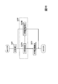
- the estimation unit 220 includes a state estimation unit 221, an observed amount estimation unit 222, and a future observed amount estimation unit 223. Further, the observed amount estimation unit 222 includes an intermediate value estimation unit 222A and an intermediate observation value estimation unit 222B.
- the state estimation unit 221 differs in the processing content between the first embodiment and the third embodiment.
- the observation amount estimation unit 222 and the future observation amount estimation unit 223 have the same processing contents in the first embodiment and the third embodiment.
- the state estimation unit 221 estimates the state from the observed amount using the encoder of the auto encoder (S221) and outputs it.
- the state estimation unit 221 receives the neural network parameter wenc and the expansion coefficient B prior to the estimation process.
- the state estimation unit 221 receives the neural network parameter w enc prior to the estimation process.
- the state estimation unit 221 estimates the state x t by sampling from the multivariate normal distribution according to ( ⁇ t , ⁇ t ).
- observation amount estimation unit 222 The observation amount estimation unit 222 estimates the observation amount from the state using the decoder of the auto encoder (S222) and outputs it.
- the process performed by the state estimation unit 221 is defined by the first function
- the process performed by the observation amount estimation unit 222 is defined by the second function
- the first function is the second function. It is an inverse function.
- the intermediate value estimation unit 222A receives the neural network parameter w dec prior to the estimation process.
- the estimated value of the reconstructed basis function value is also referred to as an intermediate value.
- the intermediate observation value estimation unit 222B receives the expansion coefficient B prior to the estimation process.
- the intermediate observed value estimation unit 222B receives the estimated value ⁇ z t as an input, estimates the observed value from the estimated value ⁇ z t (S222B), and outputs the estimated value ⁇ y t .
- ⁇ 0.
- the future observation amount estimation unit 223 receives K and B prior to the estimation process.
- the future observation amount estimation unit 223 estimates the future observation amount, which is a value in which the observation amount fluctuates over time, using the parameter K representing the time evolution (S223), and outputs it.
- estimation units 120 of the learning devices of the first and third embodiments can be similarly expressed. However, processing is performed using the learning observation amount and the learning target parameter.
- the learning device and the estimation device are configured by loading a special program into a known or dedicated computer having, for example, a central processing unit (CPU) and a main storage device (RAM: Random Access Memory). It is a special device.
- the learning device and the estimation device execute each process under the control of the central processing unit, for example.
- the data input to the learning device and the estimation device and the data obtained by each process are stored in, for example, the main storage device, and the data stored in the main storage device are read to the central processing unit as necessary. Used for other processing.
- At least a part of each processing unit of the learning device and the estimation device may be configured by hardware such as an integrated circuit.
- Each storage unit included in the learning device and the estimation device can be configured by a main storage device such as a RAM (Random Access Memory) or middleware such as a relational database or a key-value store.
- a main storage device such as a RAM (Random Access Memory) or middleware such as a relational database or a key-value store.
- middleware such as a relational database or a key-value store.
- each storage unit does not necessarily have to be provided inside the learning device and the estimation device, and is configured by an auxiliary storage device configured by a semiconductor memory device such as a hard disk, an optical disk, or a flash memory (Flash Memory), The configuration may be provided outside the device and the estimation device.
- flash Memory Flash Memory
- the program describing this processing content can be recorded in a computer-readable recording medium.
- the computer-readable recording medium may be, for example, a magnetic recording device, an optical disc, a magneto-optical recording medium, a semiconductor memory, or the like.
- Distribution of this program is carried out by selling, transferring, or lending a portable recording medium such as a DVD or a CD-ROM in which the program is recorded. Further, this program may be stored in a storage device of a server computer, and the program may be distributed by transferring the program from the server computer to another computer via a network.
- a computer that executes such a program first stores, for example, the program recorded in a portable recording medium or the program transferred from the server computer in its own storage unit. Then, when executing the process, this computer reads the program stored in its own storage unit and executes the process according to the read program. Further, as another embodiment of this program, a computer may directly read the program from a portable recording medium and execute processing according to the program. Further, each time a program is transferred from the server computer to this computer, the processing according to the received program may be executed successively.
- ASP Application Service Provider
- the program includes information used for processing by an electronic computer and equivalent to the program (data that is not a direct command to a computer but has the property of defining the processing of the computer).
- each device is configured by executing a predetermined program on a computer, at least a part of the processing contents may be realized by hardware.
Landscapes
- Engineering & Computer Science (AREA)
- Physics & Mathematics (AREA)
- Theoretical Computer Science (AREA)
- General Health & Medical Sciences (AREA)
- Computing Systems (AREA)
- Biomedical Technology (AREA)
- Biophysics (AREA)
- Computational Linguistics (AREA)
- Data Mining & Analysis (AREA)
- Evolutionary Computation (AREA)
- Life Sciences & Earth Sciences (AREA)
- Molecular Biology (AREA)
- Artificial Intelligence (AREA)
- General Engineering & Computer Science (AREA)
- General Physics & Mathematics (AREA)
- Mathematical Physics (AREA)
- Software Systems (AREA)
- Health & Medical Sciences (AREA)
- Probability & Statistics with Applications (AREA)
- Testing And Monitoring For Control Systems (AREA)
Abstract
Description
本実施形態は、時間発展と観測過程だけでなく、同時に観測過程の「逆関数」を学習することで、観測量だけから観測過程・時間発展・状態の全てを学習することを可能とする。具体的にはオートエンコーダネットワーク(参考文献1参照)を用いる。
(参考文献1)G. E. Hinton. "Reducing the Dimensionality of Data with Neural Networks", Science, 313(5786):504-507, July 2006.
xt+1 =f(xt) (1)
この状態xtから、観測量ytが観測過程、
yt=g(xt) (2)
を通じて得られる。このとき、観測量は何らかの方法で数値化されるもの(たとえば電流電圧、温度、音圧、画像など)であり、マイクロホンアレイで得られるような多次元データでもよい。
・状態の系列データ{x1,…,xT}
・時間発展の関数f(xt)
・観測過程の関数g(xt)
を決定することである。
(Koopmanモード分解)
基底関数


Ψ(xt+1)=Ψ(f(xt))= KΨ(xt) (4)
のように書き直すことができる。
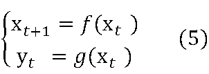

図1に本実施形態の概要を記載している。観測量の系列データ{yt}を入力とし、状態xt、観測過程(^Ψ,B)、時間発展Kを学習する。学習後はある観測量ytから予測した観測量の系列データ^y1 (t),^y2 (t),…や状態xtを出力する。

本実施形態は二段階に分かれている。一つは観測量の時系列データから時間発展と観測過程ならびにその逆関数を学習する段階(以下、学習段階ともいう)である。一つは観測量から状態を取得する段階(以下、状態取得段階ともいう)である。
図4は学習装置100の機能ブロック図を、図5はその処理フローの例を示す。学習装置100は、初期化部110、推定部120、目的関数計算部130、パラメータ更新部140とを含む。
初期化部110は、学習に先立ち、推論に用いるパラメータwenc (k),wdec (k),K(k),B(k)を初期化し(S110)、初期化したパラメータwenc (0),wdec (0),K(0),B(0)を推定部120に出力する。また、更新回数を示すインデックスkをk=0とする。
推定部120は、学習用の観測量の系列データ{yt (L)}と初期化または更新したパラメータwenc (k),wdec (k),K(k),B(k)を入力とし、(1)基底関数の値の推定(推定値zt)、(2)状態の推定(推定値xt)、(3)再構成した基底関数の値の推定(推定値^zt)、(4)基底関数の予測(予測値^zτ (t))、(5)観測量の予測(予測値^yτ (t))を行い(S120)、推定値zt、xt、^zt、予測値^zτ (t)、^yτ (t)を出力する。以下、推定および予測を合わせて推定ともいう。以下、推定の詳細を説明する。
目的関数計算部130は、学習用の観測量の系列データ{yt+τ (L)}と、推定値の系列データ{zt+τ}、{xt+τ}、{^zt+τ}、予測値の系列データ{^zτ (t)}、{^yτ (t)}、パラメータwenc (k)、wdec (k)を入力とし、目的関数の値J(Θ)を計算し(S130)、出力する。なお、Θはパラメータwenc (k),wdec (k),K(k),B(k)の集合である。


パラメータ更新部140は、目的関数J(Θ)を受け取り、各パラメータwenc (k),wdec (k),K(k),B(k)を更新する(S140)。例えば、Back propagationを用いて各パラメータに対する勾配ΔΘJを計算し、各パラメータwenc (k),wdec (k),K(k),B(k)を更新する(Θ(k+1)=Θ(k)+ΔΘJ)。
図7は推定装置200の機能ブロック図を、図8はその処理フローの例を示す。推定装置200は、推定部220を含む。
図9のアルゴリズム2を実行する場合、推定装置200は、観測量ytを入力とし、観測量ytに対応する状態を推定し、yt以降の観測量の系列データを予測し、推定値xt、予測した系列データ{^yτ (t)}を出力する。図9のアルゴリズム2では、推定部220に適当な画像データに基づくデータを観測量ytとして、Τステップ先の画像データまで予測することができる。例えば、観測量の系列データyt,yt+1,…,yt+Nを入力とし、推定値の系列データxt,xt+1,…,xt+Nと、予測したN個の系列データ{^yτ (t)},{^yτ (t+1)},…,{^yτ (t+N)}を出力してもよい。
推定部220は、観測量ytを入力とし、観測量ytに対して所定の処理を行うことで状態を推定する(S220)。本実施形態では、所定の処理は、(1)基底関数の値の推定(推定値zt)、(2)状態の推定(推定値xt)である。さらに、推定部220は、(3)再構成した基底関数の値の推定(推定値^zt)、(4)基底関数の予測(予測値^zτ (t))、(5)観測量の予測(予測値^yτ (t))を行い(S220)、推定値xt、予測値の系列データ{^yτ (t)}を出力する。
図11のアルゴリズム3を実行する場合、推定装置200は、状態xtを入力とし、状態xtに対応する観測量を予測し、予測した系列データ{^yτ (t)}を出力する。図11のアルゴリズム3では、推定部220に適当な状態xtを与え、Τステップ先の画像まで予測することができる。
学習段階では、観測量だけから観測過程・時間発展・状態を学習することができる。
本実施形態では、観測量が画像データに基づくデータの場合について説明したが、他のデータであってもよい。例えば、音響データに基づくデータ、振動データに基づくデータ、音響データに基づくデータと振動データに基づくデータとの組合せなどが考えられる。以下に、より詳しく説明する。
観測量を音響データに基づくデータとした場合、マイクから取れた音圧の波形データまたはその特徴量(STFT やlog-Mel power など)を入力ytとする。なお、マイクロホンアレイで収音する場合、音圧の波形データまたはその特徴量を素子数分だけ結合したベクトルを入力ytとする。
観測量を振動データに基づくデータとした場合、振動ピックアップから取れた加速度の波形データまたはその特徴量(STFT やlog-Melpower など)を入力ytとする。複数の振動ピックアップでの収録する場合、波形データや特徴量を素子数分だけ結合したベクトルを入力とする。
観測量を上述の音響データに基づくデータと振動データに基づくデータとの組合せとした場合、振動ピックアップから取れた加速度の波形データまたはその特徴量とマイクから取れた音圧の波形データまたはその特徴量を素子数分だけ結合したベクトルを入力ytとする。
第一実施形態と異なる部分を中心に説明する。
異常検知装置300は、誤差ベクトル計算部310と平均分散共分散行列計算部320と検知部330とを含む(図12参照)。
まず、正常時の観測量のデータセットDnormal={y1,y2,…,yT_1}を用意する。ただし、下付き添え字A_BはABを意味する。ここから,系列の長さLの部分系列Dt={yt+1,…,yt+L}、t=1,2,…,T1-Lを取り出す。

異常検知の対象となる観測量のデータセットDnew={y'1,y'2,…,yT_2}が得られたとき、前処理のときと同様に、系列の長さLの部分系列D't'={yt'+1,…,yt'+L}、t'=1,2,…,T2-Lを取り出す。
Lt'=logdet(S)+(e't'-μ)TS-1(e't'-μ)T
この異常度合いLt'は誤差ベクトルを正規分布でフィッティングしたときの負の対数尤度に比例する量である。
第一実施形態と異なる部分を中心に説明する。
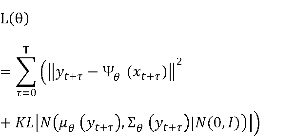
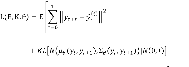
図16は学習装置100の機能ブロック図を、図5はその処理フローの例を示す。学習装置100は、初期化部110、推定部120、目的関数計算部130、パラメータ更新部140とを含む。
推定部120は、学習用の観測量の系列データ{yt}と初期化または更新したパラメータwenc (k),wdec (k),K(k),B(k)を入力とし、(1)状態の平均と分散パラメータの推定(推定値σt,μt)、(2)状態の推定(推定値xt)、(3)再構成した基底関数の値の推定(推定値^zt)、(4)基底関数の予測(予測値^zτ (t))、(5)観測量の予測(予測値^yτ (t))を行い(S120)、予測値^yτ (t)を出力する。(3)~(5)は第一実施形態と同様なので、(1),(2)について説明する。
目的関数計算部130は、学習用の観測量の系列データ{yt+τ}と、予測値の系列データ{^yτ (t)}、パラメータwenc (k)を入力とし、目的関数の値L(B(k),K(k),θ(k))を計算し(S130)、出力する。なお、θ(k)はパラメータwenc (k),wdec (k)の集合である。

図7は推定装置200の機能ブロック図を、図8はその処理フローの例を示す。推定装置200は、推定部220を含む。
観測量から状態を推定し、観測量を予測する場合(第一実施形態のアルゴリズム2の場合)、推定装置200は、観測量ytを入力とし、観測量ytに対応する状態を推定し、yt以降の観測量の系列データを予測し、推定値xt、予測した系列データ{^yτ (t)}を出力する。例えば、観測量の系列データyt,yt+1,…,yt+Nを入力とし、推定値の系列データxt,xt+1,…,xt+Nと、予測したN個の系列データ{^yτ (t)},{^yτ (t+1)},…,{^yτ (t+N)}を出力してもよい。
推定部220は、観測量ytを入力とし、観測量ytに対して所定の処理を行うことで状態を推定する(S220)。本実施形態では、所定の処理は、状態の平均と分散パラメータの推定(推定値σt,μt)、(2)状態の推定(推定値xt)である。さらに、推定部220は、(3)再構成した基底関数の値の推定(推定値^zt)、(4)基底関数の予測(予測値^zτ (t))、(5)観測量の予測(予測値^yτ (t))を行い(S220)、推定値xt、予測値の系列データ{^yτ (t)}を出力する。(3)~(5)は第一実施形態と同様なので、(1),(2)について説明する。
観測量から観測量を予測する場合(第一実施形態のアルゴリズム3の場合)、第一実施形態と同様である。
第一実施形態と同様の効果を得ることができる。生成モデルを考えることで、逆関数を考えることなく状態を推定する。なお、本実施形態と第一実施形態の変形例や第二実施形態を組合せてもよい。
第一実施形態および第三実施形態の推定部220を図17の機能ブロック図で表現することもできる。図18は推定部220の処理フローの例を示す。
状態推定部221は、オートエンコーダのエンコーダを用いて、観測量から状態を推定し(S221)、出力する。
観測量推定部222は、オートエンコーダのデコーダとを用いて、状態から観測量を推定し(S222)、出力する。
中間値推定部222Aは、推定処理に先立ちニューラルネットワークのパラメータwdecを受け取る。
中間観測値推定部222Bは、推定処理に先立ち展開係数Bを受け取る。
^zτ (t)=Kτ^zt
^yτ (t) = B^zτ (t)
つまり、^yt = B^ztである。
未来観測量推定部223は、推定処理に先立ちK、Bを受け取る。
学習装置および推定装置は、例えば、中央演算処理装置(CPU: Central Processing Unit)、主記憶装置(RAM: Random Access Memory)などを有する公知又は専用のコンピュータに特別なプログラムが読み込まれて構成された特別な装置である。学習装置および推定装置は、例えば、中央演算処理装置の制御のもとで各処理を実行する。学習装置および推定装置に入力されたデータや各処理で得られたデータは、例えば、主記憶装置に格納され、主記憶装置に格納されたデータは必要に応じて中央演算処理装置へ読み出されて他の処理に利用される。学習装置および推定装置の各処理部は、少なくとも一部が集積回路等のハードウェアによって構成されていてもよい。学習装置および推定装置が備える各記憶部は、例えば、RAM(Random Access Memory)などの主記憶装置、またはリレーショナルデータベースやキーバリューストアなどのミドルウェアにより構成することができる。ただし、各記憶部は、必ずしも学習装置および推定装置がその内部に備える必要はなく、ハードディスクや光ディスクもしくはフラッシュメモリ(Flash Memory)のような半導体メモリ素子により構成される補助記憶装置により構成し、学習装置および推定装置の外部に備える構成としてもよい。
本発明は上記の実施形態及び変形例に限定されるものではない。例えば、上述の各種の処理は、記載に従って時系列に実行されるのみならず、処理を実行する装置の処理能力あるいは必要に応じて並列的にあるいは個別に実行されてもよい。その他、本発明の趣旨を逸脱しない範囲で適宜変更が可能である。
また、上記の実施形態及び変形例で説明した各装置における各種の処理機能をコンピュータによって実現してもよい。その場合、各装置が有すべき機能の処理内容はプログラムによって記述される。そして、このプログラムをコンピュータで実行することにより、上記各装置における各種の処理機能がコンピュータ上で実現される。
Claims (7)
- エンコーダを用いて、観測量から状態を推定する状態推定部と、
前記デコーダとを用いて、状態から観測量を推定する観測量推定部と、
時間展開を表すパラメータKを用いて、前記観測量が時間推移により変動した値である未来観測量を推定する未来観測量推定部と、を有し、
前記エンコーダのパラメータと、前記デコーダのパラメータと、前記パラメータKとは、同時に最適化されたものである、
推定装置。 - 請求項1の推定装置であって、
前記状態推定部が行う処理は第一の関数で、前記観測量推定部が行う処理は第二の関数で定義され、
前記第一の関数は前記第二の関数の逆関数である、
推定装置。 - 請求項1の推定装置であって、
前記エンコーダのパラメータと、前記デコーダのパラメータと、前記パラメータKとは、前記状態推定部をエンコーダとし、前記観測量推定部をデコータとする変分オートエンコーダにより最適化されたものであり、
前記観測量は時系列観測量である、
推定装置。 - 請求項1から請求項3の何れかの推定装置であって、
前記観測量推定部は、
前記状態から中間値を推定する中間値推定部と、
推定した前記中間値から、前記観測値を推定する中間観測値推定部と、を含み、
前記未来観測量推定部は、前記パラメータKを用いて得られる、前記中間値が時間推移により変動した値である未来中間値から前記未来観測量を推定する、
推定装置。 - 請求項2の推定装置で用いるパラメータを学習する学習装置であって、
前記第二の関数は前記オートエンコーダのデコーダのパラメータである、基底関数のパラメータを用い、前記第一の関数は前記オートエンコーダのエンコーダのパラメータである、前記基底関数の逆関数のパラメータを用い、
学習用の観測量の系列データと、前記基底関数のパラメータ、前記逆関数のパラメータ、前記パラメータK、展開係数とを用いて、(1)基底関数の値の推定、(2)状態の推定、(3)再構成した基底関数の値の推定、(4)基底関数の予測、(5)観測量の予測を行う推定部と、
前記学習用の観測量の系列データと、基底関数の推定値の系列データ、状態の推定値の系列データ、再構成した基底関数の推定値の系列データ、基底関数の予測値の系列データ、観測量の予測値の系列データを用いて、(i)観測量の予測誤差、(ii)基底関数の予測誤差、(iii)前記基底関数のパラメータ、前記逆関数のパラメータに基づくニューラルネットワークの重みに対する正則化項、(iv)前記状態の構造を求め、求めた値から目的関数の値を求める目的関数計算部と、
前記目的関数に基づき、前記基底関数のパラメータ、前記逆関数のパラメータ、前記パラメータK、前記展開係数とを更新する更新部とを含み、
前記状態は非線形で時間推移するものであり、
前記観測量は状態の時間推移に伴い非線形で時間推移する観測処理を行うことで得ることができるものである、
学習装置。 - エンコーダを用いて、観測量から状態を推定する状態推定ステップと、
前記デコーダとを用いて、状態から観測量を推定する観測量推定ステップと、
時間展開を表すパラメータKを用いて、前記観測量が時間推移により変動した値である未来観測量を推定する未来観測量推定ステップと、を有し、
前記エンコーダのパラメータと、前記デコーダのパラメータと、前記パラメータKとは、同時に最適化されたものである、
推定方法。 - 請求項1から請求項4の何れかの推定装置、または、請求項5の学習装置としてコンピュータを機能させるためのプログラム。
Priority Applications (2)
| Application Number | Priority Date | Filing Date | Title |
|---|---|---|---|
| US17/425,684 US20240028872A1 (en) | 2019-01-28 | 2019-08-30 | Estimation apparatus, learning apparatus, methods and programs for the same |
| JP2020569354A JP7163977B2 (ja) | 2019-01-28 | 2019-08-30 | 推定装置、学習装置、それらの方法、およびプログラム |
Applications Claiming Priority (2)
| Application Number | Priority Date | Filing Date | Title |
|---|---|---|---|
| JP2019011981 | 2019-01-28 | ||
| JP2019-011981 | 2019-01-28 |
Publications (1)
| Publication Number | Publication Date |
|---|---|
| WO2020158032A1 true WO2020158032A1 (ja) | 2020-08-06 |
Family
ID=71840041
Family Applications (1)
| Application Number | Title | Priority Date | Filing Date |
|---|---|---|---|
| PCT/JP2019/034216 Ceased WO2020158032A1 (ja) | 2019-01-28 | 2019-08-30 | 推定装置、学習装置、それらの方法、およびプログラム |
Country Status (3)
| Country | Link |
|---|---|
| US (1) | US20240028872A1 (ja) |
| JP (1) | JP7163977B2 (ja) |
| WO (1) | WO2020158032A1 (ja) |
Cited By (1)
| Publication number | Priority date | Publication date | Assignee | Title |
|---|---|---|---|---|
| JP2022070386A (ja) * | 2020-10-27 | 2022-05-13 | 日本電信電話株式会社 | 学習方法、系列解析方法、学習装置、系列解析装置、及びプログラム |
Citations (2)
| Publication number | Priority date | Publication date | Assignee | Title |
|---|---|---|---|---|
| WO2018052875A1 (en) * | 2016-09-15 | 2018-03-22 | Google Llc | Image depth prediction neural networks |
| JP2019502212A (ja) * | 2016-01-14 | 2019-01-24 | 株式会社Preferred Networks | 時系列データ適合およびセンサ融合のシステム、方法、および装置 |
Family Cites Families (9)
| Publication number | Priority date | Publication date | Assignee | Title |
|---|---|---|---|---|
| US8095210B2 (en) * | 2007-01-19 | 2012-01-10 | California Institute Of Technology | Prosthetic devices and methods and systems related thereto |
| US10572830B2 (en) * | 2017-04-24 | 2020-02-25 | Virginia Tech Intellectual Properties, Inc. | Learning and deploying compression of radio signals |
| US11334807B1 (en) * | 2017-06-23 | 2022-05-17 | Virginia Tech Intellectual Properties, Inc. | Learning approximate estimation networks for communication channel state information |
| US20190228110A1 (en) * | 2018-01-19 | 2019-07-25 | General Electric Company | System and method for abstracting characteristics of cyber-physical systems |
| US12033080B2 (en) * | 2018-06-15 | 2024-07-09 | Google Llc | Sparse recovery autoencoder |
| US20200082272A1 (en) * | 2018-09-11 | 2020-03-12 | International Business Machines Corporation | Enhancing Data Privacy in Remote Deep Learning Services |
| WO2020064990A1 (en) * | 2018-09-27 | 2020-04-02 | Deepmind Technologies Limited | Committed information rate variational autoencoders |
| EP3667439A1 (en) * | 2018-12-13 | 2020-06-17 | ABB Schweiz AG | Predictions for a process in an industrial plant |
| US11172195B2 (en) * | 2019-01-26 | 2021-11-09 | Qualcomm Incorporated | Excluding intra coded reference samples from local illumination compensation parameter derivation |
-
2019
- 2019-08-30 JP JP2020569354A patent/JP7163977B2/ja active Active
- 2019-08-30 US US17/425,684 patent/US20240028872A1/en not_active Abandoned
- 2019-08-30 WO PCT/JP2019/034216 patent/WO2020158032A1/ja not_active Ceased
Patent Citations (2)
| Publication number | Priority date | Publication date | Assignee | Title |
|---|---|---|---|---|
| JP2019502212A (ja) * | 2016-01-14 | 2019-01-24 | 株式会社Preferred Networks | 時系列データ適合およびセンサ融合のシステム、方法、および装置 |
| WO2018052875A1 (en) * | 2016-09-15 | 2018-03-22 | Google Llc | Image depth prediction neural networks |
Non-Patent Citations (1)
| Title |
|---|
| SHIN ISHIGURO; HARUKA KIKUCHI; YUSUKE FUKAZAWA: "Taxi Demand Forecast with Stacked denoising Auto encoders Using Real-time Population Data.", TRANSACTIONS OF THE INFORMATION PROCESSING SOCIETY OF JAPAN, vol. 60, no. 1, 15 January 2019 (2019-01-15), JP, pages 118 - 128, XP009522772, ISSN: 1882-7764 * |
Cited By (2)
| Publication number | Priority date | Publication date | Assignee | Title |
|---|---|---|---|---|
| JP2022070386A (ja) * | 2020-10-27 | 2022-05-13 | 日本電信電話株式会社 | 学習方法、系列解析方法、学習装置、系列解析装置、及びプログラム |
| JP7542821B2 (ja) | 2020-10-27 | 2024-09-02 | 日本電信電話株式会社 | 学習方法、系列解析方法、学習装置、系列解析装置、及びプログラム |
Also Published As
| Publication number | Publication date |
|---|---|
| JPWO2020158032A1 (ja) | 2021-09-30 |
| JP7163977B2 (ja) | 2022-11-01 |
| US20240028872A1 (en) | 2024-01-25 |
Similar Documents
| Publication | Publication Date | Title |
|---|---|---|
| CN113239022B (zh) | 医疗诊断缺失数据补全方法及补全装置、电子设备、介质 | |
| Tang et al. | Online weighted LS-SVM for hysteretic structural system identification | |
| US20210089953A1 (en) | Quantum bit prediction | |
| Chen et al. | Genetic algorithm with an improved fitness function for (N) ARX modelling | |
| JP7542821B2 (ja) | 学習方法、系列解析方法、学習装置、系列解析装置、及びプログラム | |
| JP2022523484A (ja) | 観測値の尤度を使用して環境を探索するためのエージェントを制御すること | |
| CN111160459A (zh) | 超参数的优化装置和方法 | |
| JPWO2019215904A1 (ja) | 予測モデル作成装置、予測モデル作成方法、および予測モデル作成プログラム | |
| Li et al. | Structural damage quantification using long short-term memory (LSTM) auto-encoder and impulse response functions | |
| JP7490185B2 (ja) | 解析対象の3次元再構成装置、3次元再構成方法及び3次元再構成プログラム | |
| CN113537614A (zh) | 电网工程造价预测模型的构建方法、系统、设备及介质 | |
| JP2010092247A (ja) | 制御器、制御方法及び制御プログラム | |
| JP7163977B2 (ja) | 推定装置、学習装置、それらの方法、およびプログラム | |
| JP2019095894A (ja) | 推定装置、学習装置、学習済みモデル、推定方法、学習方法、及びプログラム | |
| JP7047665B2 (ja) | 学習装置、学習方法及び学習プログラム | |
| CN110309869A (zh) | 面向未知场景的稳定识别方法及装置 | |
| CN120562316A (zh) | 基于平衡优化的多模态轴承剩余寿命预测方法与系统 | |
| CN118839564B (zh) | 基于少量测点加速度数据和生成对抗网络的结构全自由度振型识别方法 | |
| WO2018198298A1 (ja) | パラメータ推定装置、パラメータ推定方法、及びコンピュータ読み取り可能な記録媒体 | |
| Li et al. | Pygpphs: A python package for Bayesian modeling of port-Hamiltonian systems | |
| Pastori et al. | Quantum neural networks for cloud cover parameterizations in climate models | |
| JP7672844B2 (ja) | 性能予測装置、性能予測方法及び性能予測プログラム | |
| JP2021082014A (ja) | 推定装置、訓練装置、推定方法、訓練方法、プログラム及び非一時的コンピュータ可読媒体 | |
| Wilson et al. | Hierarchical model verification and validation for structural health monitoring using dynamic substructuring | |
| JP7331938B2 (ja) | 学習装置、推定装置、学習方法及び学習プログラム |
Legal Events
| Date | Code | Title | Description |
|---|---|---|---|
| 121 | Ep: the epo has been informed by wipo that ep was designated in this application |
Ref document number: 19913132 Country of ref document: EP Kind code of ref document: A1 |
|
| ENP | Entry into the national phase |
Ref document number: 2020569354 Country of ref document: JP Kind code of ref document: A |
|
| WWE | Wipo information: entry into national phase |
Ref document number: 17425684 Country of ref document: US |
|
| NENP | Non-entry into the national phase |
Ref country code: DE |
|
| 122 | Ep: pct application non-entry in european phase |
Ref document number: 19913132 Country of ref document: EP Kind code of ref document: A1 |