WO2020086497A1 - Systems and methods for rig scheduling with optimal fleet sizing - Google Patents
Systems and methods for rig scheduling with optimal fleet sizing Download PDFInfo
- Publication number
- WO2020086497A1 WO2020086497A1 PCT/US2019/057303 US2019057303W WO2020086497A1 WO 2020086497 A1 WO2020086497 A1 WO 2020086497A1 US 2019057303 W US2019057303 W US 2019057303W WO 2020086497 A1 WO2020086497 A1 WO 2020086497A1
- Authority
- WO
- WIPO (PCT)
- Prior art keywords
- wells
- rig
- time
- drilling
- schedule
- Prior art date
- Legal status (The legal status is an assumption and is not a legal conclusion. Google has not performed a legal analysis and makes no representation as to the accuracy of the status listed.)
- Ceased
Links
Classifications
-
- G—PHYSICS
- G06—COMPUTING OR CALCULATING; COUNTING
- G06Q—INFORMATION AND COMMUNICATION TECHNOLOGY [ICT] SPECIALLY ADAPTED FOR ADMINISTRATIVE, COMMERCIAL, FINANCIAL, MANAGERIAL OR SUPERVISORY PURPOSES; SYSTEMS OR METHODS SPECIALLY ADAPTED FOR ADMINISTRATIVE, COMMERCIAL, FINANCIAL, MANAGERIAL OR SUPERVISORY PURPOSES, NOT OTHERWISE PROVIDED FOR
- G06Q50/00—Information and communication technology [ICT] specially adapted for implementation of business processes of specific business sectors, e.g. utilities or tourism
- G06Q50/02—Agriculture; Fishing; Forestry; Mining
-
- G—PHYSICS
- G06—COMPUTING OR CALCULATING; COUNTING
- G06Q—INFORMATION AND COMMUNICATION TECHNOLOGY [ICT] SPECIALLY ADAPTED FOR ADMINISTRATIVE, COMMERCIAL, FINANCIAL, MANAGERIAL OR SUPERVISORY PURPOSES; SYSTEMS OR METHODS SPECIALLY ADAPTED FOR ADMINISTRATIVE, COMMERCIAL, FINANCIAL, MANAGERIAL OR SUPERVISORY PURPOSES, NOT OTHERWISE PROVIDED FOR
- G06Q10/00—Administration; Management
- G06Q10/06—Resources, workflows, human or project management; Enterprise or organisation planning; Enterprise or organisation modelling
- G06Q10/063—Operations research, analysis or management
- G06Q10/0631—Resource planning, allocation, distributing or scheduling for enterprises or organisations
- G06Q10/06313—Resource planning in a project environment
-
- G—PHYSICS
- G06—COMPUTING OR CALCULATING; COUNTING
- G06Q—INFORMATION AND COMMUNICATION TECHNOLOGY [ICT] SPECIALLY ADAPTED FOR ADMINISTRATIVE, COMMERCIAL, FINANCIAL, MANAGERIAL OR SUPERVISORY PURPOSES; SYSTEMS OR METHODS SPECIALLY ADAPTED FOR ADMINISTRATIVE, COMMERCIAL, FINANCIAL, MANAGERIAL OR SUPERVISORY PURPOSES, NOT OTHERWISE PROVIDED FOR
- G06Q10/00—Administration; Management
- G06Q10/06—Resources, workflows, human or project management; Enterprise or organisation planning; Enterprise or organisation modelling
- G06Q10/063—Operations research, analysis or management
- G06Q10/0631—Resource planning, allocation, distributing or scheduling for enterprises or organisations
- G06Q10/06314—Calendaring for a resource
Definitions
- the rig scheduling problem concerns finding a schedule for a fleet of rigs given a list of potential wells to be drilled.
- Each rig has a capacity and time period of availability, while each well comprises a production value, a pad assignment and a time window in which it can be drilled.
- Operational constraints limit the number of rigs on a pad to one, and the moving and dismantling time is applicable each time a rig moves from one pad to another. There is a need for an improved method for optimizing resources.
- Figure 1 illustrates pseudo code for weight scoring method according to embodiments of the present disclosure.
- Figure 2 illustrates pseudo code for the Greedy method according to embodiments of the present dislcosure.
- Figure 3 illustrates pseudo code for a scheduling algorithm according to embodiments of the present disclosure.
- Figure 4 is a schematic diagram illustrating systems and methods for optimizing rig scheduling according to embodiments of the present disclosure.
- Figure 5 is a schematic diagram depicting an optimizing algorithm according to embodiments of the present disclosure.
- Figure 6 is a schematic block diagram showing a method according to embodiments of the present disclosure.
- Figure 7 is a schematic block diagram of a method according to further embodiments of the present disclosure.
- Figure 8 illustrates pseudo code for a fast greedy method according to embodiments of the present disclosure.
- Embodiments of the present disclosure are directed to a method including receiving a list of wells to be drilled and dividing the wells into ON wells which have a specific start date of availability, BY wells which have a fixed end date of availability but no start date of availability; and ADD wells which have no start or end data of availability.
- Availability in this context generally means that the well is available to be accessed and/or drilled.
- the method also includes receiving fleet data, wells data, and parameters, wherein the parameters include a time horizon for the drilling operation.
- the method also includes attempting to solve an integer problem according to the ON wells, and if the integer problem is solved, implementing a greedy method for BY wells and a weight scoring method for ADD wells. If the integer problem is not solved, the method continues by implementing the weight scoring method for all wells, and outputting a schedule for rigs and the wells.
- the greedy method may include sorting wells according to the earliest day on which the wells are available and then by a value of the wells, and for each rig available to drill, identifying an earliest start date and assigning a rig to the start date for the well.
- the weight scoring method may include identifying urgent wells.
- An urgent well is a well in which the earliest time to start drilling the well is earlier than the earliest time a rig is available, when factoring in the cost of using the rig and a moving cost for the rig.
- the method also includes identifying non urgent wells.
- a non-urgent well has a potential start date such that there is an available start date for at least one rig that is earlier than the earliest available date for the well.
- the method also includes randomly choosing weights, repeatedly calculating a solution using weights generated by the weights, and retaining a solution that maximizes an objective value of the solution. If there is no improvement of the objective value of the solution after a
- the method continues by ceasing calculating the solution and delivering the retained solution.
- Urgent wells are given higher priority than non-urgent wells.
- Other embodiments are directed to a method for optimizing fleet scheduling, including identifying ON wells which have a beginning time of availability, BY wells which have an end time but no beginning time of availability, and ADD wells which have no beginning or end time of availability, according to ON, BY, and ADD constraints.
- the method also includes scheduling rigs to drill the wells with ON wells having higher priority than BY wells, and with BY wells having higher priority than ADD wells, and returning a schedule for rigs and wells, the schedule having a value corresponding to a number of ON, BY, and ADD constraints which are satisfied by the schedule.
- Still further embodiments of the present disclosure are directed to a system for optimizing a rig schedule for drilling a plurality of wells.
- the system includes a scheduler configured to receive fleet data, wells data, and solving parameters.
- the scheduler is configured to identify according to time constraints in the wells data: wells that have a beginning date of availability as ON wells, wells that have an end date but no beginning date of availability as BY wells, and wells that have no beginning or end date of availability as ADD wells.
- the scheduler is further configured to solve an integer problem for ON wells, a greedy method for BY wells, and a weight scoring method for ADD wells, and to output a schedule having a score, wherein the score pertains to how many of the time constraints are satisfied by the schedule. If the integer problem is not solved in a predetermined time period the scheduler is configured to implement the weight scoring method for all wells.
- the system also includes an optimizer configured to iteratively pass the fleet data, wells data, and solving parameters to the scheduler and to optimize based on the score.
- the rig scheduling problem concerns finding a schedule for a fleet of rigs given a list of potential wells to be drilled.
- Each rig has a capacity and time period of availability, while each well comprises a production value, a pad assignment and a time window in which it can be drilled.
- Operational constraints limit the number of rigs on a pad to one, and the moving and dismantling time is applicable each time a rig moves from one pad to another.
- a narrow or restricted time window identifies wells with strong conditions imposed by client needs. That is, wells that must be drilled on or by certain days, often in order to retain lease rights.
- the critical assumption in the procedure is firstly, to meet the satisfiable stipulated conditions, and secondly, to maximize the production value of the selected wells.
- the fleet-sizing procedure can be used to identify how many additional rigs are required by type and period of use to meet the outstanding conditions, or to provide the optimal fleet size to meet the satisfiable conditions from the outset when no fleet is given.
- the proposed decomposition-based scheme is presented in this report with several practical test cases.
- This value can be anything ranging from barrels of oil to net value generated by the well in $. This pre-computed fixed value should be defined with the purpose of being maximized.
- a "pad” is a location from which one or multiple wells are drilled. When installed on a pad, a rig can drill multiple wells without being dismantled. Most importantly, on any given day, there can only be a single rig on a given pad (a rig is considered to be on a pad from the first day of its installation to the last day of its dismantling). Finally there are P pads numbered from 1 to P , ard denotes the set of wells on pad .
- a well can have timing requirements where T refers to a time period of interest.
- w (resp. ) is the first (resp. last) day when is available to be drilled. If and w then w is referred to as a "BY" well. If then w is referred to as a "ON well. If w is neither ON or BY, then it is assumed that 1 and is referred to as an "ADD" well.
- ⁇ ON ⁇ BY ⁇ ADD the sets 0 f ON, BY and ADD wells.
- each well w belongs to a pad P .
- the maximum time between two pads is relatively small compared to 24 hours (1 day) and hence can be neglected.
- the reason for this is that a "day” is the unit of measure of the rig capacity, installation and dismantling times.
- the resulting schedule will be very sensitive to external factors (delays due to traffic, weather for instance) and will not be robust.
- (resp. ) is the first (resp. last) day when r is available to be used.
- r (resp. ® r ) corresponds to the number of days required to install r on (resp. dismantle r from) a pad (see below for the definition of a pad) and ⁇ r ⁇ r + ⁇ >r defines the moving time of r .
- the first goal of the operator should be to maximize the number of time requirements that can be met given the aforementioned constraints. Given a schedule the number of constraints met is equal to the number
- a "good" schedule should aim to maximize the production value.
- the production value of a schedule is the sum of the production values of all the selected wells in and is denoted by
- the objective function may be defined as:
- the problem can be solved by formulating an integer program taking into account all types of wells (ON, BY and ADD) in conjunction with an appropriate solver (Cbc for open-source, Gurobi or CPIex if available).
- an appropriate solver Cbc for open-source, Gurobi or CPIex if available.
- This method is a myopic method based on a scoring function computed with a set of weights. Note that in the following, tr - w defines a function that depends on r and w , so we can use tsy to refer to the case s 1 r and V 1 M .
- Scoring function is a function of w the potential well to drill, tr the earliest available day of rig r , t r,w ...t r the earliest day to drill well w with rig r . It is denoted by .
- - ⁇ 1 is the normalized value of the well w . It gives a positive value to wells with high value:
- J 2 is the normalized difference between the earliest available day of r and the end date of w . It emphasizes wells that have time constraints:
- - ⁇ 3 is the negative normalized idle time of rig r . It gives preference to wells that do not require the rig r to stand idle:
- - ⁇ 4 is the normalized function of rig requirements. It gives emphasis to wells that are highly constrained by rig requirements:
- Urgent Wells A well w is urgent at time r for rig r if w r r r and urgentWells is the set of such wells. If urgentWells is not empty, consider the most urgent well w in this set. If w can be assigned to a different rig than r with less idle time than r or with same idle time but greater rig capacity, then do so and remove w from urgentWells. If not, assign w to the schedule of r and skip the next step. If all wells from urgentWells are assigned to other rigs than r , consider the next step.
- Non-Urgent Wells For all wells with a potential start date tr - w such that t r,w e K ⁇ ⁇ ⁇ + C r +M r 1 ⁇ C0
- Figure 1 illustrates pseudo code for weight scoring method according to embodiments of the present disclosure.
- Pseudo code in this disclosure is to be understood to represent embodiments of how a method can be implemented. It is to be understood that there are alternative methods for coding and virtually limitless ways to code a given method and the present disclosure is not limited to the particulars of the pseudo code.
- the methods can include to rank the wells lexicographically first by end date, then by value, and then to check if the highest ranked well can be added to the schedule by finding the earliest start drilling day when the well j,E
- Figure 2 illustrates pseudo code for the Greedy method according to embodiments of the present dislcosure.
- Phase ON integer program for ON wells (IPON), WS, G.
- Phase BY G, WS.
- Phase ADD WS, G.
- IPON Integer Program for ON wells
- Pad incompatibilities this is the set of pairs of wells ⁇ ’ v ) that cannot be drilled by the two distinct rigs r 1 . If two wells are on the same pad and their dates are "too" close, they cannot be drilled by two different rigs. That is, if two ON wells are on the same pad and their dates differ by less than the minimum rig capacity, it will be impossible to drill both wells. This is defined as follows:
- T solve be the time in seconds specified by the user to solve the scheduling problem.
- Figure S illustrates pseudo code for a scheduling algorithm according to embodiments of the present disclosure.
- FIG. 4 is a schematic diagram 10 illustrating systems and methods for optimizing rig scheduling according to embodiments of the present disclosure.
- To schedule a rig fleet certain characterists are identified and an order of priority is assigned to the characteristics.
- certain wells have constraints which may come from the lease of the land, access to the wellsite, geopolitical factors, or virtually any other constraint upon the timing of access to the well site.
- the wells are first grouped into three groups: "ON”, “BY”, and "ADD".
- ON wells are wells which must be drilled on a given day or days. These are the highest priority because they are the least flexible.
- BY wells are wells with an end date of availability and as such must be drilled "by" a certain date.
- ADD wells includes all other wells that are not ON or BY wells. These wells are the third and lowest priority because they may be drilled anytime. In many cases there is a global end date to the drilling period in question, and this global end date is factored into calculations in addition to the other parameters.
- the processes and methods illustrated in Figure 4 can be executed by a scheduler 11.
- the scheduler takes as input: 1) a fleet data 12, which can include such parameters as R rigs, each with a capacity C r , start day T r1 , end day T r2 , installation I r and dismantling D r time.
- the scheduler also receives well data 14 which may include W wells to be drilled with a production value V w , a pad P w , a start day T ws , an end day T wE and a set of permissible rigs w .
- the scheduler 11 also receives a set of parameters 16 which may include the time horizon of T days and solver parameters such as the time specified by the user to solve the scheduling problem T solve r the convergence criteria for ⁇ method and the integer program solver. With these inputs, the scheduler 11 first solves IRON is for ON wells 17. IRON 18 is an integer problem which is an attempt to solve the problem. It is possible for the constraints to be managable and the IRON is is solvable in which case the overall endeavor of scheduling the rig is simplified. If it is solved within a certain optimality gap (
- the scheduler 11 is configured to schedule wells in order of priority ON > BY > ADD, with other parameters such as production value having a lesser priority.
- Test Case B with 0/0. Firstly, 6 inconsistencies are identified (6 of type rig). The resulting schedule drills 585 wells with 42 out of 48 ON wells and 9 out of 9 BY wells met, giving
- Test Case B with 3/2. Firstly, 7 inconsistencies are identified (7 of type rig). The resulting schedule drills 585 wells with 41 out of 48 ON wells and 9 out of 9 BY wells met, giving
- N(S) 50 .
- V(S) 3.69 x 10 ®
- test case A inconsistencies and num ber of conditions. This state leads to the development of optimal fleet sizing in the next section.
- the first input is an upper bound on the number of additional rigs L u .
- the list of hireable rigs is given by type of rigs. There are D types of rigs and each type of rig / e ⁇ l,..., A ⁇ js g jven with:
- a minimum hiring period m minimum number of days for which the rig has to
- a hiring cost m cost incurred just to hire a new rig of type specified in the same unit as the value of a well.
- ⁇ An operating cost : cost incurred per day of utilization of a rig of type ⁇ , also specified in the same unit as the value of a well.
- This solution can be represented by an array of size RAdd X ⁇ .
- RAdd X ⁇ the type of the additional rigs can be expressed in a vector of integers of length represents a new fleet of one
- the objective is slightly different from different from the previous section.
- the objective according to embodiments of the present disclosure is to find a new fleet F - (X, a , a ) a nc
- nint(.) is the nearest integer function.
- Figure 5 is a schematic diagram depicting an optimizing algorithm according to embodiments of the present disclosure.
- An optimization routine such as a genetic algorithm (GA), a meta heuristic such as Tabu Search or Simulated Annealing, or any other suitable optimization routine can be used.
- the optimization routine is performed by an optimizer 32.
- the optimization routine developed for the sizing problem takes as input fleet data 12, wells data 14, and other parameters 16.
- the optimizer 32 also receives new rig data 34 which holds
- the parameter file includes the parameters of the scheduler 11 as well as parameters for the optimization routine including the population size, the mutation probability, a convergence criteria and the total solving time.
- C(F) F scheduler is used together with the cost 38 to establish the fitness value for each ' .
- the optimization routine's operations are then applied to the population and this process repeats until the solving time or the convergence criteria is met.
- the optimizer 32 outputs the best fleet F 28' and its associated schedule ⁇ F ) ( a nc
- Test B1 and Test B2 do not require any fleet sizing as the resulting schedule meets the maximum number of constraints (including the inconsistencies). Therefore, we focus here on Test A1 and Test A2.
- Test Case A1 with R Md 1.
- the resulting fleet consists of one rig of type 1 from 29- Apr-2016 to 24-Oct-2016.
- Test Case A1 with R Md 2.
- the resulting fleet consists of one rig of type 1 from 9- Apr-2016 to 20-Nov-2016.
- Test Case A2 with R Md 1.
- the resulting fleet consists of one rig of type 1 from 1- May-2016 to 19-Oct-2016.
- the resulting fleet consists of one rig of type 1 from 2- Apr-2016 to 26- May-2017 and one rig of type 2 from 2-Apr-2016 to 26- May-2017.
- the resulting schedule drills 250 wells with 39 out of 41 ON wells and 55 out of 55 BY wells met, giving terms 0 f va
- FIG. 6 is a schematic block diagram showing a method 40 according to embodiments of the present disclosure.
- the parameters can be any salient parameter and includes fleet data and well data.
- the fleet data pertains to the fleet of rigs, the capacity, availability, cost of operating, moving, hiring the rigs, etc.
- Wells data includes time constraints for the wells.
- the parameters can also include the solution parameters such as convergence criteria and any other suitable parameter which may be needed.
- ON wells are identified. ON wells are wells which have a restrictive time window in which they must be drilled. In some cases, there are a few hours or a few days only in which the well can be drilled. The ON wells generally have a starting and ending availability window and as such are the most restrictive.
- BY wells are identified. BY wells are wells which must be drilled "by" a certain date/time. BY wells therefore have an ending availability time, but no beginning availability time. These wells are less restrictive than ON wells.
- ADD wells are identified. ADD wells can be simply the remainder of all wells, less ON and BY wells. Generally ADD wells have no time constraints upon when they can be drilled and as such are less restrictive than ON and BY wells.
- the method includes scheduling rigs with ON wells having higher priority than BY wells, and BY wells having higher priority than ADD wells. The method can also output a schedule for the rigs having a score, wherein the score pertains to how well or poorly the time constraints from which the ON, BY, and ADD designations are created.
- FIG. 7 is a schematic block diagram of a method 60 according to further embodiments of the present disclosure.
- parameters are collected. This portion can be similar to 42 of the method 40 depicted in Figure 6.
- the method 60 can also identify ON, BY, and ADD wells also in a similar manner.
- an integer problem for the ON wells is attempted. For some sets of data there is a simple solution and this attempt will produce a meaningful solution that does not require intensive computing.
- the method includes applying the weight scoring method for all wells at 68. If, on the other hand, the integer problem is solved, at 70 the greedy method (or fast greedy method) is used for BY wells, and at 72 the weight scoring method is used for ADD wells.
- a schedule is output by the method which includes a schedule and a score that pertains to how well or poorly the schedule meets the ON, BY, and ADD criteria.
- This method has three steps. First we select wells for each rig using an integer program. Then these wells are inserted (ON then BY then ADD in a greedy manner) rig-by-rig. Finally it tries to insert additional wells in the idle times that were not selected in the first step.
- D solves the following integer program. For clarity, we define ⁇ ⁇ w + ⁇ ON ⁇ Xmax» ⁇ _ we also define D to be the set of incompatible wells to be drilled by the same rig (see rig inconsistencies).
- IPADD Integer Program for ADD wells
- PADD the set of pads with at least one ADD well. Given the resulting schedule from the BY phase, we can identify "slots" in which wells can be drilled.
- a slot s corresponding to rig r has 4 attributes:
- Tt a start date, i.e. the day after the rig stopped drilling the previous well.
- slot 5 of rig r is selected for slot 5 of rig r ; then it should be placed continuously with the pad (i.e. at the beginning or the end of the slot). Subsequently, the order of the other pads within a given slot does not affect the quality of the solution in this setting, as well as the order of wells within a pad.
- the systems and methods of the present disclosure are directed to new approaches to the rig scheduling problem based on a number of decomposition and approximation schemes. Many algorithms were described and combined into a composite procedure with the aim of addressing the satisfiable conditions while maximizing the production value of the selected wells. In some applications there are conditions that cannot be met which is due to
- the method also provides the means to establish the optimal fleet size required to satistfy the outstanding requirements and increase the overall production value. Future considerations include improving the mutation operator of the genetic algorithm for sizing and considering the possibility of using generic time windows for all wells.
Landscapes
- Business, Economics & Management (AREA)
- Human Resources & Organizations (AREA)
- Engineering & Computer Science (AREA)
- Economics (AREA)
- Strategic Management (AREA)
- Entrepreneurship & Innovation (AREA)
- Tourism & Hospitality (AREA)
- Theoretical Computer Science (AREA)
- General Physics & Mathematics (AREA)
- Marketing (AREA)
- General Business, Economics & Management (AREA)
- Physics & Mathematics (AREA)
- Game Theory and Decision Science (AREA)
- Quality & Reliability (AREA)
- Operations Research (AREA)
- Educational Administration (AREA)
- Development Economics (AREA)
- Life Sciences & Earth Sciences (AREA)
- Agronomy & Crop Science (AREA)
- Biodiversity & Conservation Biology (AREA)
- Animal Husbandry (AREA)
- Marine Sciences & Fisheries (AREA)
- Mining & Mineral Resources (AREA)
- Health & Medical Sciences (AREA)
- General Health & Medical Sciences (AREA)
- Primary Health Care (AREA)
- Management, Administration, Business Operations System, And Electronic Commerce (AREA)
- Stored Programmes (AREA)
Abstract
Systems and methods for optimizing oilfield rig fleet scheduling and deployment are disclosed. Wells are identified to have time constraints by which they are grouped into "ON", "BY", and "ADD" categories. ON wells have a beginning drilling availability window; BY wells have an ending drilling availability time only; and ADD wells have no beginning or ending time of drilling availability. The systems and methods optimize scheduling with ON wells having higher priority than BY wells, and BY wells having higher priority than ADD wells.
Description
SYSTEMS AND METHODS FOR RIG SCHEDULING WITH OPTIMAL FLEET SIZING
CROSS REFERENCE PARAGRAPH
[0001] This application claims the benefit of U.S. Non-Provisional Application No. 16/166,267, entitled "SYSTEMS AND METHODS FOR RIG SCHEDULING WITH OPTIMAL FLEET SIZING," filed October 22, 2018, the disclosure of which is hereby incorporated herein by reference.
BACKGROUND
[0002] For oilfield drilling operations, the rig scheduling problem concerns finding a schedule for a fleet of rigs given a list of potential wells to be drilled. Each rig has a capacity and time period of availability, while each well comprises a production value, a pad assignment and a time window in which it can be drilled. Operational constraints limit the number of rigs on a pad to one, and the moving and dismantling time is applicable each time a rig moves from one pad to another. There is a need for an improved method for optimizing resources.
BRIEF DESCRIPTION OF THE FIGURES
[0003] Figure 1 illustrates pseudo code for weight scoring method according to embodiments of the present disclosure.
[0004] Figure 2 illustrates pseudo code for the Greedy method according to embodiments of the present dislcosure.
[0005] Figure 3 illustrates pseudo code for a scheduling algorithm according to embodiments of the present disclosure.
[0006] Figure 4 is a schematic diagram illustrating systems and methods for optimizing rig scheduling according to embodiments of the present disclosure.
[0007] Figure 5 is a schematic diagram depicting an optimizing algorithm according to embodiments of the present disclosure.
[0008] Figure 6 is a schematic block diagram showing a method according to embodiments of the present disclosure.
[0009] Figure 7 is a schematic block diagram of a method according to further embodiments of the present disclosure.
[0010] Figure 8 illustrates pseudo code for a fast greedy method according to embodiments of the present disclosure.
SUMMARY
[0011] Embodiments of the present disclosure are directed to a method including receiving a list of wells to be drilled and dividing the wells into ON wells which have a specific start date of availability, BY wells which have a fixed end date of availability but no start date of availability; and ADD wells which have no start or end data of availability. Availability in this context generally means that the well is available to be accessed and/or drilled. The method also includes receiving fleet data, wells data, and parameters, wherein the parameters include a time horizon for the drilling operation. The method also includes attempting to solve an integer problem according to the ON wells, and if the integer problem is solved, implementing a greedy method for BY wells and a weight scoring method for ADD wells. If the integer problem is not solved, the method continues by implementing the weight scoring method for all wells, and outputting a schedule for rigs and the wells.
[0012] The greedy method may include sorting wells according to the earliest day on which the wells are available and then by a value of the wells, and for each rig available to drill, identifying an earliest start date and assigning a rig to the start date for the well. The weight scoring method may include identifying urgent wells. An urgent well is a well in which the earliest time to start drilling the well is earlier than the earliest time a rig is available, when factoring in the cost of using the rig and a moving cost for the rig. The method also includes identifying non urgent wells. A non-urgent well has a potential start date such that there is an available start date for at least one rig that is earlier than the earliest available date for the well. The method also includes randomly choosing weights, repeatedly calculating a solution using weights
generated by the weights, and retaining a solution that maximizes an objective value of the solution. If there is no improvement of the objective value of the solution after a
predetermined number of attempts, the method continues by ceasing calculating the solution and delivering the retained solution. Urgent wells are given higher priority than non-urgent wells.
[0013] Other embodiments are directed to a method for optimizing fleet scheduling, including identifying ON wells which have a beginning time of availability, BY wells which have an end time but no beginning time of availability, and ADD wells which have no beginning or end time of availability, according to ON, BY, and ADD constraints. The method also includes scheduling rigs to drill the wells with ON wells having higher priority than BY wells, and with BY wells having higher priority than ADD wells, and returning a schedule for rigs and wells, the schedule having a value corresponding to a number of ON, BY, and ADD constraints which are satisfied by the schedule.
[0014] Still further embodiments of the present disclosure are directed to a system for optimizing a rig schedule for drilling a plurality of wells. The system includes a scheduler configured to receive fleet data, wells data, and solving parameters. The scheduler is configured to identify according to time constraints in the wells data: wells that have a beginning date of availability as ON wells, wells that have an end date but no beginning date of availability as BY wells, and wells that have no beginning or end date of availability as ADD wells. The scheduler is further configured to solve an integer problem for ON wells, a greedy method for BY wells, and a weight scoring method for ADD wells, and to output a schedule having a score, wherein the score pertains to how many of the time constraints are satisfied by the schedule. If the integer problem is not solved in a predetermined time period the scheduler is configured to implement the weight scoring method for all wells. The system also includes an optimizer configured to iteratively pass the fleet data, wells data, and solving parameters to the scheduler and to optimize based on the score.
DETAILED DESCRIPTION
[0015] The rig scheduling problem concerns finding a schedule for a fleet of rigs given a list of potential wells to be drilled. Each rig has a capacity and time period of availability, while each well comprises a production value, a pad assignment and a time window in which it can be drilled. Operational constraints limit the number of rigs on a pad to one, and the moving and dismantling time is applicable each time a rig moves from one pad to another. Notably, a narrow or restricted time window identifies wells with strong conditions imposed by client needs. That is, wells that must be drilled on or by certain days, often in order to retain lease rights. For this reason, the critical assumption in the procedure is firstly, to meet the satisfiable stipulated conditions, and secondly, to maximize the production value of the selected wells. Significantly, the fleet-sizing procedure can be used to identify how many additional rigs are required by type and period of use to meet the outstanding conditions, or to provide the optimal fleet size to meet the satisfiable conditions from the outset when no fleet is given. The proposed decomposition-based scheme is presented in this report with several practical test cases.
[0016] Wells
[0017] Consider a well
 . First
 is assigned a "production value" denoted by
. This value can be anything ranging from barrels of oil to net value generated by the well in $. This pre-computed fixed value should be defined with the purpose of being maximized.
p
[0018] In addition,
 is part of a "pad" denoted by w . A "pad" is a location from which one or multiple wells are drilled. When installed on a pad, a rig can drill multiple wells without being dismantled. Most importantly, on any given day, there can only be a single rig on a given pad (a rig is considered to be on a pad from the first day of its installation to the last day of its dismantling). Finally there are P pads numbered from 1 to P , ard
 denotes the set of wells on pad
 .
.
[0019] A well can have timing requirements where T refers to a time period of interest. w (resp. ) is the first (resp. last) day when is available to be drilled. If
 and
w then w is referred to as a "BY" well. If then w is referred to as a "ON well. If w is neither ON or BY, then it is assumed that
and
w then w is referred to as a "BY" well. If then w is referred to as a "ON well. If w is neither ON or BY, then it is assumed that
 1 and is referred to as an "ADD" well. We denote ^ON ^BY ^ADD the sets 0f ON, BY and ADD wells.
[0020] Finally, some wells can only be drilled by specific rigs so we denote the set of rigs that can drill w by
 Equivalently,
 is the set of wells that rig r can potentially drill.
[0021] No transportation assumption
[0022] As previously mentioned, each well w belongs to a pad P . In this paper, it is assumed that the maximum time between two pads is relatively small compared to 24 hours (1 day) and hence can be neglected. The reason for this is that a "day" is the unit of measure of the rig capacity, installation and dismantling times. By incorporating transportation times of the order of hours, the resulting schedule will be very sensitive to external factors (delays due to traffic, weather for instance) and will not be robust.
[0023] More formally, it is possible, though not mandatory, to provide a position for each pad
 d( n, q) = (x - x )2 + (y - y )2
can be » p q P I ). Furthermore, one can suppose a speed for the trucks transporting the rigs denoted by s . The validity of the no transportation time assumption can be checked by the condition:
 denotes the maximum travel time.
[0024] The current model assumes no transportation time. Note that, if the transportation times are constant between any two pads and even multiple of days, then it can be
incorporated as follows: add half of time in the installation and half in the dismantling time of each rig. If the transportation times are of the order of the day but differ between pads, then this model would have to be modified.
[0025] Data
[0026] In summary, the input data from the user is:
[0027] 1. The time horizon considered which leads to the number of days for the required schedule.
[0028] 2. The rig information with each capacity, start and end days, installing and dismantling times in days.
[0029] 3. The well information with each value, pad, start and end days.
[0030] 4. The truck speed and maximum travel time to check the no-transportation time assumption.
[0031] The notations are summarized in the following table:


[0033] (resp. ) is the first (resp. last) day when r is available to be used. Finally, r (resp. ®r ) corresponds to the number of days required to install r on (resp. dismantle r from) a pad (see below for the definition of a pad) and ^ r ^r + ^>r defines the moving time of r .
[0034] Objective function
[0035] As the reason for time constraints imposed by the client are unclear to the operator, the first goal of the operator should be to maximize the number of time requirements that can be met given the aforementioned constraints. Given a schedule
 the number of constraints met is equal to the number

denoted by NON (S) + NBr (S) Secondly, a "good" schedule should aim to maximize the production value. The production value of a schedule is the sum of the production values of all the selected wells in and is denoted by

[0036] According to embodiments of the present disclosure, the objective function may be defined as:
max(N(S\V(S ))
[0037]
[0038] and can be optimized lexicographically, i.e., firstly ^(S)
 maximized and then
V(S)
[0039] Note: this is equivalent to optimize the single objective function ^ x ^(8) + V(S) where V is an upper bound on
 for all schedule . However, for the ease of notation we will keep the vector notation.
[0040] Inconsistencies
[0041] If the rig fleet was large enough and conditions are satisfiable, the best schedule
N(S) =1 W I + I W I
should have ’ 1 0N 1 1 BY 1 . However this may not be possible due to inconsistencies in the input data. Preferably, these inconsistencies should be corrected by the user before solving the problem. There are two types of inconsistencies.
[0042] Pad inconsistencies
[0043] Consider a pad P G i ^ - - - P} such that
 l> 1 _ Consider each pair
(w ¹ v) e Wp GL YON rj-<S rj- S
of distinct wells in pad P such that w” v . If:

[0045] then either w or v cannot be drilled due to a pad inconsistency. In other words, if w has to be drilled before v , but their drilling time is not separated by at least the best rig capacity (the smallest one) that can drill w .
[0046] Rig inconsistencies and each pair
 distinct wells such that

[0049] where % is the indicator function, then either w or v cannot be drilled due to a rig inconsistency.
[0050] Algorithms
[0051] In some embodiments the problem can be solved by formulating an integer program taking into account all types of wells (ON, BY and ADD) in conjunction with an appropriate solver (Cbc for open-source, Gurobi or CPIex if available). However, this solution appears to be intractable due to the curse of dimensionality, that is, the problem size becomes too large to solve for a high number of wells and rigs.
[0052] In order to bypass this issue, one can adopt one of two schemes detailed below:
[0053] 1. An approximation scheme.
[0054] 2. A decomposition scheme.
[0055] Approximation Algorithms
[0056] In this case, all wells are considered by a sub-optimal algorithm which gives the smallest optimality gap. Two such algorithms are considered:
[0057] · A "weight scoring" algorithm with sub-functionals denoted by WS.
[0058] · A "greedy" mechanism denoted by G.
[0059] Note that two other algorithms (called fastGreedy and Dual) that were studied are explained in the Appendix.
[0060] Weight scoring (WS) method
[0061] This method is a myopic method based on a scoring function computed with a set of weights. Note that in the following, tr-w defines a function that depends on r and w , so we can use tsy to refer to the case s ¹ r and V ¹ M .
[0062] Scoring function
 , the scoring function is a function of w the potential well to drill, tr the earliest available day of rig r , t r,w ...t r the earliest day to drill well w with rig r . It is denoted by
 .
.

[0066] and the sub-functionals
 a re descrjbed as follows:
[0067] -^1 is the normalized value of the well w . It gives a positive value to wells with high value:
V.
/l O) =
max{Vw, }
[0068] (2)
[0069] J 2 is the normalized difference between the earliest available day of r and the end date of w . It emphasizes wells that have time constraints:

[0071] -^3 is the negative normalized idle time of rig r . It gives preference to wells that do not require the rig r to stand idle:
 [0073] -^4 is the normalized function of rig requirements. It gives emphasis to wells that are highly constrained by rig requirements:

[0075] Given a set of weights ? , one approach according to embodiments of the present disclosure for ^ works as follows:
[0076] Let
 be the earliest time for which at least one rig is available. Let r be such a rig with highest capacity.
t TE < t + C + M
[0077] 1. Urgent Wells: A well w is urgent at time r for rig r if w r r r and urgentWells is the set of such wells. If urgentWells is not empty, consider the most urgent well w in this set. If w can be assigned to a different rig than r with less idle time than r or with same idle time but greater rig capacity, then do so and remove w from urgentWells. If not, assign w to the schedule of r and skip the next step. If all wells from urgentWells are assigned to other rigs than r , consider the next step.
[0078] 2. Non-Urgent Wells : For all wells with a potential start date tr-w such that t r,w e K· · ·· + Cr +Mr 1 } C0|T|pUte t e scorjng function
 | nsert in the rigSchedule, the well w such that
 js maximized.
[0079] Figure 1 illustrates pseudo code for weight scoring method according to embodiments of the present disclosure. Pseudo code in this disclosure is to be understood to represent embodiments of how a method can be implemented. It is to be understood that there are alternative methods for coding and virtually limitless ways to code a given method and the present disclosure is not limited to the particulars of the pseudo code.
[0080] Weight Optimization
[0081] An astute reader will notice that the resulting schedule depends on the set of weights y used to compute the scoring function. However the optimal set of weights may not be known. Therefore the WS method considers a random search in the space of weights and retains the solution that maximizes the objective value. There is a convergence criteria on this
search process: if there is no improvement of the best solution after a certain number of evaluations ( k <º N then the search stops.
[0082] Note: a genetic algorithm approach was also implemented but the random weight procedure proved to be as effective with fewer evaluations.
[0083] Greedy (G) method
[0084] According to embodiments of the present disclosure, the methods can include to rank the wells lexicographically first by end date, then by value, and then to check if the highest ranked well can be added to the schedule by finding the earliest start drilling day when the well j,E
is available ( L w’ w J ). The process can be repeated until the list of wells is empty. The pseudo code of the method is given below. [H]
[0085] Figure 2 illustrates pseudo code for the Greedy method according to embodiments of the present dislcosure.
[0086] Note that this method was designed to work fine for "BY" wells. However, it can also be used on a different set of wells with varying performance.
[0087] Decomposition
[0088] In other embodiments another solution to the approximation scheme is to consider wells separately by type. That is, consider constrained wells (ON and BY) and then ADD wells. Among constrained wells, since ON wells are more constrained, it seems appropriate that they should be treated first. Hence, consider three phases, comprising the set of ON then BY and finally, ADD wells. In this scheme, one can use ^ and approximation schemes described above, or alternatively an integer program, such as the one detailed below. In summary, we list the possible algorithms in preference order for each phase as follows:
[0089] 1. Phase ON: integer program for ON wells (IPON), WS, G.
[0090] 2. Phase BY: G, WS.
[0091] 3. Phase ADD: WS, G.
[0092] Note that an integer program tested for ADD wells is presented in the Appendix.
However it did not prove as effective as the WS or G schemes.
[0093] Integer Program for ON wells (IPON)
[0094] The goal is to find a combination of ON wells in order to maximize the number of ON wells drilled. Note there can exist several such combinations, hence we differentiate the solutions by selecting the one with highest production value.
K. = V... HI QXw'eW,
[0095] Let us define an "artificial" value K as: ON K' } and describe two incompatibility sets as follows:
[0096] 1. Rig incompatibilities ( !n 1 )-: this is the set of pairs of wells (w,v) that cannot be drilled by the same rig r , i.e. among the pairs in
 only one element can be drilled by
 Mathematically, this requirement is defined by:

[0098] 2. Pad incompatibilities
 : this is the set of pairs of wells ^’v) that cannot be drilled by the two distinct rigs r ¹ . If two wells are on the same pad and their dates are "too" close, they cannot be drilled by two different rigs. That is, if two ON wells are on the same pad and their dates differ by less than the minimum rig capacity, it will be impossible to drill both wells. This is defined as follows:

[0100] The only variable is
[0101] xwr e {0,1 }: 1 if well w is drilled by rig r e Rw
[0102] We can formulate the IP as follows:

[0108] Solving this problem, we get the solution for the ON phase which gives an allocation of all possible ON wells to rigs that meet the given constraints (e.g. rig, pad, time windows, etc)
[0109] Scheduling algorithm
[0110] Given all these algorithms, the proposed solution was chosen after testing the different methods on different test cases and is described below algorithmically.
[0111] Let Tsolve be the time in seconds specified by the user to solve the scheduling problem.
[0112] Figure S illustrates pseudo code for a scheduling algorithm according to embodiments of the present disclosure.
[0113] Rig Schedule
[0114] Figure 4 is a schematic diagram 10 illustrating systems and methods for optimizing rig scheduling according to embodiments of the present disclosure. To schedule a rig fleet certain characterists are identified and an order of priority is assigned to the characteristics. In some embodiments certain wells have constraints which may come from the lease of the land, access to the wellsite, geopolitical factors, or virtually any other constraint upon the timing of access to the well site. The wells are first grouped into three groups: "ON", "BY", and "ADD". ON wells are wells which must be drilled on a given day or days. These are the highest priority because they are the least flexible. BY wells are wells with an end date of availability and as such must be drilled "by" a certain date. These are the second highest priority because there is more flexibility to the wells. If scheduling permits these wells can be drilled earlier than their "by" date, but not later. ADD wells (short for "additional") includes all other wells that are not ON or BY wells. These wells are the third and lowest priority because they may be drilled anytime. In many cases there is a global end date to the drilling period in question, and this global end date is factored into calculations in addition to the other parameters.
[0115] The processes and methods illustrated in Figure 4 can be executed by a scheduler 11. The scheduler takes as input: 1) a fleet data 12, which can include such parameters as R rigs, each with a capacity C r , start day T r1 , end day T r2 , installation I r and dismantling D r time. The scheduler also receives well data 14 which may include W wells to be drilled with a production value V w, a pad P w, a start day T ws , an end day T wE and a set of permissible rigs w . The scheduler 11 also receives a set of parameters 16 which may include the time horizon of T days and solver parameters such as the time specified by the user to solve the
scheduling problem Tsolve r the convergence criteria for ^ method and the integer program solver. With these inputs, the scheduler 11 first solves IRON is for ON wells 17. IRON 18 is an integer problem which is an attempt to solve the problem. It is possible for the constraints to be managable and the IRON is is solvable in which case the overall endeavor of scheduling the rig is simplified. If it is solved within a certain optimality gap (
I W0N | xmax„{^} ) ; then BY wells 19 are treated by the O 20 method and ADD wells 22 with the WS 24 method. If IRON 18 was not solved, the scheduler 11 treats all wells using the S 26 method. (The ^ 26 method and ^ 24 method can be the same method.) The scheduler 11 outputs a schedule 28, the number of constraints met by 28 denoted by (S) and the total production value of the wells selected by 28 denoted by
 .
.
[0116] Accordingly, the scheduler 11 is configured to schedule wells in order of priority ON > BY > ADD, with other parameters such as production value having a lesser priority.
[0117] The following information was obtained using actual simulations and test data and is included to show certain features of the present disclosure and is not given in a limiting manner. Parameters and values are given here to show some test data but the scope of the present disclosure is not limited to the numerical values or relationships.
[0118] Data
[0119] The two data sets (representative of real test cases) are presented in Table 2.

[0120] Table 2: Data summary of two test cases
[0121] Note that the wells have different rigs requirements. Moreover, the rigs do not have the same start and end dates. We consider both test cases with identical rig installing/dismantling times of 0/0 and 3/2, giving a total of 4 test cases.
[0122] 2.4.2 Results
[0123] Note that Tsolve = 60s a ncj the so|ver used was Cbc (expect for test case B with 3/2 where Tsolve = 300s ) Results are summarized in Table 3.
[0124] Test Case A1
[0125] : Test Case A with 0/0. Firstly, 2 inconsistencies are identified (1 of type pad and 1 of type rig). The resulting schedule drills 259 wells with 37 out of 41 ON wells and 55 out of 55 BY wells met, giving (S) 92 In terms of value, V(S) = l .8l x l06
[0126] Test Case A2
[0127] : Test Case A with 3/2. Firstly, 2 inconsistencies are identified (1 of type pad and 1 of type rig). The resulting schedule drills 225 wells with 35 out of 41 ON wells and 55 out of 55 BY wells met, giving (S) 90 In terms of value, V(S) = 1.59 x 10®
[0128] Test Case B1
[0129] : Test Case B with 0/0. Firstly, 6 inconsistencies are identified (6 of type rig). The resulting schedule drills 585 wells with 42 out of 48 ON wells and 9 out of 9 BY wells met, giving
^(^) - 5l . |n terms of value,

[0130] Test Case B2
[0131] Test Case B with 3/2. Firstly, 7 inconsistencies are identified (7 of type rig). The resulting schedule drills 585 wells with 41 out of 48 ON wells and 9 out of 9 BY wells met, giving
N(S) = 50 . In terms of value, V(S) = 3.69 x 10®

[0133] Note that, in test case B, inconsistencies and (S) sum up to
 I which indicates that the solution provided is the best given the data available (in terms of constraints).
[0134] In test case A, inconsistencies and
 number of conditions. This state leads to the development of optimal fleet sizing in the next section.
[0135] Fleet sizing
[0136] As shown in the previous section, some constraints may not be met due to the lack of rigs. Moreover, in the case where no rigs are owned, one may be interested in sizing a potential fleet to drill the given list of wells. This section aims to address these concerns.
[0137] Problem Description
[0138] New data
[0139] As per to the original problem, there is a list of wells to drill and a fixed fleet of rigs which has a cost equal to 0 . In addition, there are potential rigs to hire.
Add
[0140] The first input is an upper bound on the number of additional rigs L u . In addition, the list of hireable rigs is given by type of rigs. There are D types of rigs and each type of rig / e { l,..., A} js gjven with:
CA e N
[0141] · A capacity m
NA e N NA
[0142] · A number of rigs available m : at most m rigs of type ^ can be added.
IA eN
[0143] · An installation time m [0144] · A dismantling time

A
pe ^ cannot be hired earlier than m (
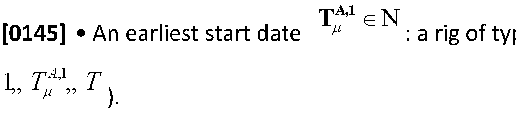
nA,2 :N •A,2 A,
T:
[0146] · An end date : a rig of type ^ can be hired until p i’ T m T .
M G N
[0147] · A minimum hiring period m : minimum number of days for which the rig has to
MA Ta’2 -Ta’1 TA’2 -Ma + 1
be hired ( m" m m ). So the latest start date is m m
A,h
[0148] · A hiring cost m : cost incurred just to hire a new rig of type
 specified in the same unit as the value of a well.
[0149] · An operating cost
 : cost incurred per day of utilization of a rig of type ^ , also specified in the same unit as the value of a well.
[0150] New fleet
R = o
[0151] If Add , the problem is equivalent to the scheduling problem of the previous section and the scheduling algorithm solves the problem.
? E N R
[0152] Given Add , an additional fleet of Add rigs is defined as follows: for each
r e { ! , ... , RAdd }
additional rig , the solution must specify:
[0153] · The type of r ,
 , where ^ r ^ means that r is not selected to be added as an additional rig.
d r.. i. „ '
[0154] · The hiring start date
d2 TA’2 d2 -d .. Mu A
[0155] · The hiring end date G” m such that Ar . The cost incurred is equal to

[0156] This solution can be represented by an array of size RAdd X ^ . Now, we simplify the representation of the new fleet for the solver. First, the type of the
 additional rigs can be expressed in a vector of integers of length
 represents a new fleet of one
n — n
rig of type 1 and one rig of type 2 for Add ). Given Add and D and
 , we can map each vector of types to a unique integer X (see a mapping example in Table 4).


[0157] Table 4: Mapping example for ^Add
 (NA, NA , NA) = (2,1,1) .
[0158] In addition,
 can be mapped uniquely to another vector ^a^ ar ) e ['-’Ί] such that:
[0159]

[0160]

[0161] Therefore a new fleet is defined by a vector ^ - (X,er ,er ) 0f size l + 2RAdd _ The main advantage of this representation is that the genetic algorithm (GA) described below can be implemented without constraints, while taking into account all the new fleet constraints such as number of new rigs, start/end dates and minimum hiring time. It also reduces the number of variables
[0162] Finally, note that given a fleet F t we can pre-compute its cost
 .
.
[0163] New objective
[0164] The objective is slightly different from different from the previous section. The objective according to embodiments of the present disclosure is to find a new fleet F - (X, a , a ) a nc| an associated schedule $(F) such that we maxj m jze firstly the number of time constraints met denoted by
 and then the net value defined
 - C(F)
mathematically that is:
[0165]
 [0166] Genetic Algorithm
[0167] Given a fixed fleet and a new fleet F , the inner maximization can be solved using the scheduling algorithm described in the previous section. In order to deal with the outer maximization on ^ , we use a genetic algorithm scheme. In order to use this scheme, the user specifies:
[0168] 1. RAdd : number of additional rigs considered.
[0169] 2. The population size.
[0170] 3. The mutation probability.
[0171] 4. A convergence criteria: if after a certain number of iterations, the best solution is not improved, the search stops.
[0172] 5. The solving time permitted for the genetic algorithm.
[0173] 6. The parameters of the scheduling algorithm, that is Tsolve r the MIP solver and the convergence criteria for WS .
[0174] We describe here the crossover and mutation operators.
[0175] Crossover
[0176] Given a population, we select the top half with the highest objective function values. The crossover operator selects randomly two distinct elements from this pool. In order to
Fx = {X,a\a2)
crossover and
 , the resulting fleet F3 = (z,r r 2)
 that:
that:
[0177] 1. Draw ^ uniformly at random in [1 / 4, 3 / 4] a nc| Z nint(/ IX + (1 Z)7)

[0179] (a) Draw l uniformly at random in [1 / 4>3 / 4] and r' = mnt( a + l)b ) . [0180] (b) Draw ^ uniformly at random in [1 / 4>3 / 4] and
 _
_
[0181] where nint(.) is the nearest integer function.
[0182] Mutation
[0183] Given the mutation probability, for each element of the population, draw a Bernoulli random variable with this probability. If it is true, then draw randomly a new element.
[0184] Note that X 1 in the new fleet F is equivalent of not adding any additional fleet. Hence, the result of the scheduling algorithm is the same as before and independent of
(a , a ) Therefore, the GA permits a new fleet with X = \ at most once in the initial population or after crossover and mutation.
[0185] Figure 5 is a schematic diagram depicting an optimizing algorithm according to embodiments of the present disclosure. An optimization routine such as a genetic algorithm (GA), a meta heuristic such as Tabu Search or Simulated Annealing, or any other suitable optimization routine can be used. The optimization routine is performed by an optimizer 32.
The optimization routine developed for the sizing problem takes as input fleet data 12, wells data 14, and other parameters 16. The optimizer 32 also receives new rig data 34 which holds
CA NA
the types of rigs available for hire with a capacity m , the number of rigs available m , the
A J)A g ' Ά,I installation time m , the dismantling time m , the earliest start date
 , the end date m ,
MA CA’h CA’°
a minimum hiring period m , a hiring cost m and an operating cost m . The parameter file includes the parameters of the scheduler 11 as well as parameters for the optimization routine including the population size, the mutation probability, a convergence criteria and the total solving time. With these inputs, we generate a population of fleets
 36 . For each
 , the algorithm generates the fleet data 12' as input to the scheduler 11. The output from the
C(F) F scheduler is used together with the cost 38 to establish the fitness value for each ' .
The optimization routine's operations (crossover and mutation) are then applied to the population and this process repeats until the solving time or the convergence criteria is met.
The optimizer 32 outputs the best fleet F 28' and its associated schedule {F ) (a nc| other metric such that N(S(F )) V(S(F )) a nc| C(F ) y
[0186] Results
[0187] Recall that both cases Test B1 and Test B2 do not require any fleet sizing as the resulting schedule meets the maximum number of constraints (including the inconsistencies). Therefore, we focus here on Test A1 and Test A2.
[0188] We summarize the new rigs data as follows:

[0189] Table 5: Additional rigs
— i
[0190] We run the two cases A1 and A2 with
 ’ which results in four cases:
[0191] Test Case Al/1
[0192] : Test Case A1 with RMd = 1. The resulting fleet consists of one rig of type 1 from 29- Apr-2016 to 24-Oct-2016. The resulting schedule drills 269 wells with 39 out of 41 ON wells and
55 out of 55 BY wells met, giving
 the production value is
1.86x1o6 the cost incurred is 0.09x10® which results in a net value of 1-77x10®.
[0193] Test Case Al/2
[0194] : Test Case A1 with RMd = 2. The resulting fleet consists of one rig of type 1 from 9- Apr-2016 to 20-Nov-2016. The resulting schedule drills 273 wells with 39 out of 41 ON wells and
55 out of 55 BY wells met, giving
 t e production value is 1.88x10®, the cost incurred is 0.11x10® which results in a net value of 1-77x10®
[0195] Test Case A2/1
[0196] : Test Case A2 with RMd = 1. The resulting fleet consists of one rig of type 1 from 1- May-2016 to 19-Oct-2016. The resulting schedule drills 233 wells with 38 out of 41 ON wells and 55 out of 55 BY wells met, giving ^(S) ~ 93 n terms 0f value, the production value is 1.60x10®, the cost incurred is 0.09x10® which results in a net value of 1-51x10®
[0197] Test Case A2/2
[0198] Test Case A2 with RMd = 2. The resulting fleet consists of one rig of type 1 from 2- Apr-2016 to 26-May-2017 and one rig of type 2 from 2-Apr-2016 to 26-May-2017. The resulting schedule drills 250 wells with 39 out of 41 ON wells and 55 out of 55 BY wells met, giving
 terms 0f va |Ue, the production value is 1.73 x lO6 t ,e cost jncurred is 0.38x l06 which results in a net value of 1-35 x lO6 _
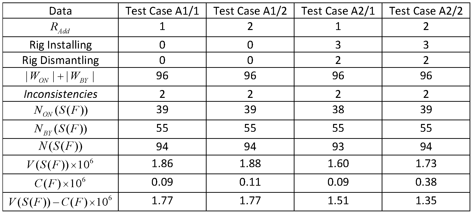
[0199] Table 6: Results summary
[0200] We find that in the case of 0/0 installing/dismantling times, one additional rig is sufficient to meet the total number of satisfiable constraints. That is,
 and the inconsistencies sum to the total number of conditions. In the case of 3/2 installing/dismantling times, two rigs are required to meet all conditions, which reduces the net value significantly.
[0201] Three methods developed and tested, but not retained in the overall scheme, are presented in this section.
[0202] Figure 6 is a schematic block diagram showing a method 40 according to embodiments of the present disclosure. At 42 parameters are collected. The parameters can be any salient parameter and includes fleet data and well data. The fleet data pertains to the fleet of rigs, the capacity, availability, cost of operating, moving, hiring the rigs, etc. Wells data includes time constraints for the wells. The parameters can also include the solution parameters such as convergence criteria and any other suitable parameter which may be needed. At 44 ON wells
are identified. ON wells are wells which have a restrictive time window in which they must be drilled. In some cases, there are a few hours or a few days only in which the well can be drilled. The ON wells generally have a starting and ending availability window and as such are the most restrictive. At 46 BY wells are identified. BY wells are wells which must be drilled "by" a certain date/time. BY wells therefore have an ending availability time, but no beginning availability time. These wells are less restrictive than ON wells. At 48 ADD wells are identified. ADD wells can be simply the remainder of all wells, less ON and BY wells. Generally ADD wells have no time constraints upon when they can be drilled and as such are less restrictive than ON and BY wells. At 50 the method includes scheduling rigs with ON wells having higher priority than BY wells, and BY wells having higher priority than ADD wells. The method can also output a schedule for the rigs having a score, wherein the score pertains to how well or poorly the time constraints from which the ON, BY, and ADD designations are created.
[0203] Figure 7 is a schematic block diagram of a method 60 according to further embodiments of the present disclosure. At 62 parameters are collected. This portion can be similar to 42 of the method 40 depicted in Figure 6. The method 60 can also identify ON, BY, and ADD wells also in a similar manner. At 64 an integer problem for the ON wells is attempted. For some sets of data there is a simple solution and this attempt will produce a meaningful solution that does not require intensive computing. At 66 if the integer problem is not solved, the method includes applying the weight scoring method for all wells at 68. If, on the other hand, the integer problem is solved, at 70 the greedy method (or fast greedy method) is used for BY wells, and at 72 the weight scoring method is used for ADD wells. At 74 a schedule is output by the method which includes a schedule and a score that pertains to how well or poorly the schedule meets the ON, BY, and ADD criteria.
[0204] Method 1: Fast Greedy (FG) method
[0205] This method is very similar to Greedy as it ranks wells based on their end dates ( w ) and their values ( ^ ) lexicographically. The main difference occurs in the process of incorporating wells into the rig Schedule. Instead of considering wells one at a time, Fast Greedy steps through time and for every day a rig is available, it tries to slot a well in the schedule of this rig (where potential wells are considered in the aforementioned ranked order).
[0206] Figure 8 illustrates pseudo code for a fast greedy method according to embodiments of the present disclosure.
[0207] Method 2: Dual (D) method
[0208] This method has three steps. First we select wells for each rig using an integer program. Then these wells are inserted (ON then BY then ADD in a greedy manner) rig-by-rig. Finally it tries to insert additional wells in the idle times that were not selected in the first step.
[0209] 1: Well Selection
[0210] In order to select a subset of potential "good" wells for each rig, D solves the following integer program. For clarity, we define ^ ^w + ^ON ^ Xmax»·^} _ we also define D to be the set of incompatible wells to be drilled by the same rig (see rig inconsistencies).

[0220] 2: Preassigned Wells Insertion
[0221] For each rig r , we get from the previous step a list of wells pre-assigned to r , that is
{w e {l,... , W} \ Xwr = l } V
. Given all these wells and rig r , we use the greedy method using as indicative value of well w to slot wells in the schedule of r . We repeat this step for each
rig r . Note that some of pre-assigned wells are not assigned to r and these are put in the pool of unassigned wells.
[0222] For each rig r :
[0223] ·
 js a set 0f preassigned wells to rig r .
[0224] · Given this pre-assignment, allocate
 wells from this set using the greedy method.
[0225] · Given this allocation of
 wells, allocate
 wells using the greedy method.
[0226] · Finally allocate
 wells using the greedy method.
[0227] 3: Unassigned Wells Insertion
[0228] Given the schedule obtained in Step 2, we have a set of unassigned wells U we use a modified greedy algorithm to try to slot the wells from the set U _ First, we rank the wells in U by value. For each well
 we check if it can be inserted in the schedule of rig r by sliding the pre-assigned wells if possible. If w cannot be assigned it is removed from ^ . This operation is repeated until U \s empty.
[0229] Method 3: Integer Program for ADD wells (IPADD)
[0230] We define PADD as the set of pads with at least one ADD well. Given the resulting schedule from the BY phase, we can identify "slots" in which wells can be drilled. A slot s corresponding to rig r has 4 attributes:
[0231] 1. Tt : a start date, i.e. the day after the rig stopped drilling the previous well.
[0232] 2. TZ : an end date, i.e. the day before the rig starts drilling another well
p pC __
[0233] 3. rs : the pad on which the previous well was drilled (0 if rs )
PF TF == H
[0234] 4. rs : the pad on which the next well is drilled (0 if rs )
[0235] Given a rig r , a slot is eligible depending on the following rules:
 TF _ TC + M Pc = 0 PF = 0
[0237] · If " r r and one of the three conditions: rs or rs or
Pc F pF
[0238] Given a rig r , let S. be the set of eligible slots for this rig with its 4 features.
[0239] We define
 to be the incompatible set of slots. Given two distinct rigs r ¹ cl and two slots
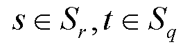 such that they "overlap", we only allow a pad to be drilled within one of these time slots but not both in order to avoid pad conflicts. Mathematically, we state:

[0241] The two types of variables are
[0242] x,„, e {0.1 }: 1 if well w e WADD is drilled by rig r e i?win slots' e Sr
[0243] yprs e {0, 1 }: 1 if p ad p e PADD is drilled by rig r e i?in slots e Sr
[0244] We formulate the IP as follows:

v = PF I D
y " . Recall that r and r are the rig installing and dismantling times of r .
[0252] This problem provides the allocation of wells to slots. Note that if a well from pad P' pF
or rs is selected for slot 5 of rig r ; then it should be placed continuously with the pad (i.e. at the beginning or the end of the slot). Subsequently, the order of the other pads within a
given slot does not affect the quality of the solution in this setting, as well as the order of wells within a pad.
[0253] The systems and methods of the present disclosure are directed to new approaches to the rig scheduling problem based on a number of decomposition and approximation schemes. Many algorithms were described and combined into a composite procedure with the aim of addressing the satisfiable conditions while maximizing the production value of the selected wells. In some applications there are conditions that cannot be met which is due to
inconsistencies in the data or due to the lack of rig capacity. For the latter, the method also provides the means to establish the optimal fleet size required to satistfy the outstanding requirements and increase the overall production value. Future considerations include improving the mutation operator of the genetic algorithm for sizing and considering the possibility of using generic time windows for all wells.
Claims
1. A method, comprising:
receiving a list of wells to be drilled;
dividing the wells into ON wells which have a specific start date of drilling availability, BY wells which have a fixed end date of drilling availability but no start date of drilling availability; and ADD wells which have no start or end data of drilling availability;
receiving fleet data, wells data, and parameters, wherein the parameters include a time horizon for the drilling operation;
attempting to solve an integer problem according to the ON wells;
if the integer problem is solved, implementing a greedy method for BY wells and a weight
scoring method for ADD wells; and
if the integer problem is not solved, implementing the weight scoring method for all wells; and outputting a schedule for rigs and the wells.
2. The system of claim 1 wherein the greedy method comprises:
sorting wells according to the earliest day on which the wells are available to be drilled and then by a value of the wells;
for each rig available to drill, identifying an earliest start date and assigning a rig to the start date for the well.
3. The system of claim 1 wherein the weight scoring method comprises:
identifying urgent wells, wherein an urgent well is a well in which the earliest time to start
drilling the well is earlier than the earliest time a rig is available for drilling, when factoring in the cost of using the rig and a moving cost for the rig;
identifying non-urgent wells, wherein a non-urgent well has a potential start date such that there is an available start date for at least one rig that is earlier than the earliest available date for the well;
randomly choosing weights;
repeatedly calculating a solution using weights generated by the weights;
retaining a solution that maximizes an objective value of the solution;
if there is no improvement of the objective value of the solution after a predetermined number of attempts, ceasing calculating the solution and delivering the retained solution, wherein urgent wells are given higher priority than non-urgent wells.
4. The method of claim 1 wherein the parameters further include a time for solving the integer problem.
5. The method of claim 1 wherein the parameters further include a convergence criteria for the integer problem.
6. The method of claim 1 wherein the parameters further include a convergence criteria for the weight scoring method.
7. The method of claim 1 wherein the parameters further include a convergence criteria for the greedy method.
8. The method of claim 1 wherein the parameters further include at least one of capacity, number of rigs available, installation time, dismantling time, earliest start date, end date, minimum hiring period, hiring cost, and operating cost.
9. The method of claim 1, further comprising deploying the rigs according to the schedule.
10. A method for optimizing fleet scheduling, comprising:
identifying ON wells which have a beginning time of drilling availability, BY wells which have an end time but no beginning time of drilling availability, and ADD wells which have no beginning or end time of drilling availability, according to ON, BY, and ADD constraints; scheduling rigs to drill the wells with ON wells having higher priority than BY wells, and with BY wells having higher priority than ADD wells;
returning a schedule for rigs and wells, the schedule having a value corresponding to a number of ON, BY, and ADD constraints which are satisfied by the schedule.
11. The method of claim 10, further comprising factoring in value of the wells at a lower priority than the ON, BY, or ADD constraints.
12. The method of claim 10, further comprising implementing a genetic algorithm to optimize the value of the schedule.
IB. The method of claim 10, further comprising factoring in installation time, dismantling time, hiring cost, operating cost, and transport time to the value, each at a lower priority than ON, BY, or ADD constraints.
14. The method of claim 10, further comprising calculating a cost according to the schedule, and factoring in the cost to the value of the schedule.
15. The method of claim 10, further comprising deploying the rigs according to the schedule.
16. A system for optimizing a rig schedule for drilling a plurality of wells, comprising:
a scheduler configured to receive fleet data, wells data, and solving parameters, the scheduler being configured to identify according to time constraints in the wells data:
wells that have a beginning date of drilling availability as ON wells; wells that have an end date but no beginning date of drilling availability as BY wells; and
wells that have no beginning or end date of drilling availability as ADD wells; the scheduler being further configured to solve an integer problem for ON wells, a greedy
method for BY wells, and a weight scoring method for ADD wells, and to output a schedule having a score, wherein the score pertains to how many of the time constraints are satisfied by the schedule, wherein if the integer problem is not solved in a predetermined time period the scheduler is configured to implement the weight scoring method for all wells;
an optimizer configured to iteratively pass the fleet data, wells data, and solving parameters to the scheduler and to optimize based on the score.
17. The system of claim 16 wherein the greedy method comprises sorting wells according to the earliest day on which the wells are available for drilling and then by a value of the wells;
and for each rig available to drill, identifying an earliest start date and assigning a rig to the start date for the well.
18. The system of claim 16 wherein the weight scoring method comprises:
randomly choosing weights;
repeatedly calculating a solution using weights generated by the weights;
retaining a solution that maximizes an objective value of the solution;
if there is no improvement of the objective value of the solution after a predetermined number of attempts, ceasing calculating the solution and delivering the retained solution.
19. The system of claim 18 wherein the weight scoring method further comprises:
identifying urgent wells, wherein an urgent well is a well in which the earliest time to start drilling the well is earlier than the earliest time a rig is available, when factoring in a cost of using the rig and a moving cost for the rig;
identifying non-urgent wells, wherein a non-urgent well has a potential start date such that there is an available start date for at least one rig that is earlier than the earliest available date for the well; and
giving higher priority to urgent wells than non-urgent wells.
20. The system of claim 18 wherein the weights pertain to a drilling availability of wells.
Applications Claiming Priority (2)
| Application Number | Priority Date | Filing Date | Title |
|---|---|---|---|
| US16/166,267 US11321788B2 (en) | 2018-10-22 | 2018-10-22 | Systems and methods for rig scheduling with optimal fleet sizing |
| US16/166,267 | 2018-10-22 |
Publications (1)
| Publication Number | Publication Date |
|---|---|
| WO2020086497A1 true WO2020086497A1 (en) | 2020-04-30 |
Family
ID=70280889
Family Applications (1)
| Application Number | Title | Priority Date | Filing Date |
|---|---|---|---|
| PCT/US2019/057303 Ceased WO2020086497A1 (en) | 2018-10-22 | 2019-10-22 | Systems and methods for rig scheduling with optimal fleet sizing |
Country Status (2)
| Country | Link |
|---|---|
| US (1) | US11321788B2 (en) |
| WO (1) | WO2020086497A1 (en) |
Families Citing this family (1)
| Publication number | Priority date | Publication date | Assignee | Title |
|---|---|---|---|---|
| US12586023B2 (en) | 2017-10-06 | 2026-03-24 | Schlumberger Technology Corporation | Dynamic balancing of well construction and well operations planning and rig equipment total cost of ownership |
Citations (5)
| Publication number | Priority date | Publication date | Assignee | Title |
|---|---|---|---|---|
| US20040220846A1 (en) * | 2003-04-30 | 2004-11-04 | Cullick Alvin Stanley | Stochastically generating facility and well schedules |
| US20080288226A1 (en) * | 2000-02-22 | 2008-11-20 | Gurpinar Omer M | Integrated Resevoir optimization |
| US20150267524A1 (en) * | 2013-06-06 | 2015-09-24 | International Business Machines Corporation | Selecting and optimizing oil field controls for production plateau |
| US20150294258A1 (en) * | 2014-04-12 | 2015-10-15 | Schlumberger Technology Corporation | Method and System for Prioritizing and Allocating Well Operating Tasks |
| WO2017058089A1 (en) * | 2015-10-01 | 2017-04-06 | Atlas Copco Rock Drills Ab | Method and system for assigning tasks to drill rigs |
Family Cites Families (1)
| Publication number | Priority date | Publication date | Assignee | Title |
|---|---|---|---|---|
| US8655705B2 (en) * | 2010-01-13 | 2014-02-18 | Lockheed Martin Corporation | Systems, methods and apparatus for implementing hybrid meta-heuristic inventory optimization based on production schedule and asset routing |
-
2018
- 2018-10-22 US US16/166,267 patent/US11321788B2/en active Active
-
2019
- 2019-10-22 WO PCT/US2019/057303 patent/WO2020086497A1/en not_active Ceased
Patent Citations (5)
| Publication number | Priority date | Publication date | Assignee | Title |
|---|---|---|---|---|
| US20080288226A1 (en) * | 2000-02-22 | 2008-11-20 | Gurpinar Omer M | Integrated Resevoir optimization |
| US20040220846A1 (en) * | 2003-04-30 | 2004-11-04 | Cullick Alvin Stanley | Stochastically generating facility and well schedules |
| US20150267524A1 (en) * | 2013-06-06 | 2015-09-24 | International Business Machines Corporation | Selecting and optimizing oil field controls for production plateau |
| US20150294258A1 (en) * | 2014-04-12 | 2015-10-15 | Schlumberger Technology Corporation | Method and System for Prioritizing and Allocating Well Operating Tasks |
| WO2017058089A1 (en) * | 2015-10-01 | 2017-04-06 | Atlas Copco Rock Drills Ab | Method and system for assigning tasks to drill rigs |
Also Published As
| Publication number | Publication date |
|---|---|
| US20200126165A1 (en) | 2020-04-23 |
| US11321788B2 (en) | 2022-05-03 |
Similar Documents
| Publication | Publication Date | Title |
|---|---|---|
| CN114239951B (en) | Satellite measurement and control task scheduling method, device and equipment based on hierarchical optimization | |
| US8799046B2 (en) | Dispatching prioritized jobs at multiple locations to workers | |
| Freeman et al. | An iterative approach for case mix planning under uncertainty | |
| US7786935B2 (en) | Method and system for inferring a location of a mobile computing device | |
| CN104881581A (en) | IoT (Internet of Things) data high-efficiency analysis method | |
| CN104834751A (en) | Data analysis method based on Internet of things | |
| CN110389817B (en) | Scheduling method, device and computer readable medium of multi-cloud system | |
| WO2022129631A1 (en) | Solving mixed integer programs using neural networks | |
| Liu et al. | Route-reduction-based dynamic programming for large-scale satellite range scheduling problem | |
| Furlan et al. | BFO: a hybrid bees algorithm for the multi-level capacitated lot-sizing problem | |
| Amirian et al. | A hybrid integer grey programming for an integrated problem of project selection and scheduling with interval data | |
| CN120547632A (en) | A wireless network resource allocation method based on edge intelligence | |
| WO2020086497A1 (en) | Systems and methods for rig scheduling with optimal fleet sizing | |
| Sun et al. | Selective maintenance on a multi‐state system considering maintenance task assignment and operating cost | |
| Eirgash | Resource allocation and leveling in construction management projects with resource histogram | |
| Yan et al. | Data-driven dynamic optimization for real-time parking reservation considering parking unpunctuality | |
| US20210103872A1 (en) | System and method for adaptive and dynamic pricing of self-storage storage units | |
| CN103713852A (en) | Method for processing information, service platform and electronic devices | |
| CN107784548A (en) | Order processing method and apparatus | |
| Nieuwoudt et al. | Algorithms for a shared resource scheduling problem in which some level of conflict is tolerable | |
| Okada et al. | A genetic algorithm with local search using activity list characteristics for solving resource‐constrained project scheduling problem with multiple modes | |
| Nguyen et al. | Integrated home health care optimization via genetic algorithms and mathematical programming | |
| Chen et al. | An approach to optimal web service composition based on QoS and user preferences | |
| Ahmed et al. | Selection, acquisition, and allocation of manufacturing technology in a multi-period environment | |
| US20240028990A1 (en) | Multi-depot vehicle scheduling |
Legal Events
| Date | Code | Title | Description |
|---|---|---|---|
| 121 | Ep: the epo has been informed by wipo that ep was designated in this application |
Ref document number: 19875699 Country of ref document: EP Kind code of ref document: A1 |
|
| NENP | Non-entry into the national phase |
Ref country code: DE |
|
| 122 | Ep: pct application non-entry in european phase |
Ref document number: 19875699 Country of ref document: EP Kind code of ref document: A1 |