WO2018213607A1 - Computerized rendering of objects having anisotropic elastoplasticity for codimensional frictional contact - Google Patents
Computerized rendering of objects having anisotropic elastoplasticity for codimensional frictional contact Download PDFInfo
- Publication number
- WO2018213607A1 WO2018213607A1 PCT/US2018/033226 US2018033226W WO2018213607A1 WO 2018213607 A1 WO2018213607 A1 WO 2018213607A1 US 2018033226 W US2018033226 W US 2018033226W WO 2018213607 A1 WO2018213607 A1 WO 2018213607A1
- Authority
- WO
- WIPO (PCT)
- Prior art keywords
- codimensional
- particles
- grid
- elastic
- deformation
- Prior art date
- Legal status (The legal status is an assumption and is not a legal conclusion. Google has not performed a legal analysis and makes no representation as to the accuracy of the status listed.)
- Ceased
Links
Classifications
-
- G—PHYSICS
- G06—COMPUTING OR CALCULATING; COUNTING
- G06T—IMAGE DATA PROCESSING OR GENERATION, IN GENERAL
- G06T13/00—Animation
- G06T13/20—Three-dimensional [3D] animation
-
- G—PHYSICS
- G06—COMPUTING OR CALCULATING; COUNTING
- G06F—ELECTRIC DIGITAL DATA PROCESSING
- G06F30/00—Computer-aided design [CAD]
- G06F30/20—Design optimisation, verification or simulation
- G06F30/23—Design optimisation, verification or simulation using finite element methods [FEM] or finite difference methods [FDM]
-
- G—PHYSICS
- G06—COMPUTING OR CALCULATING; COUNTING
- G06T—IMAGE DATA PROCESSING OR GENERATION, IN GENERAL
- G06T15/00—Three-dimensional [3D] image rendering
- G06T15/005—General purpose rendering architectures
-
- G—PHYSICS
- G06—COMPUTING OR CALCULATING; COUNTING
- G06F—ELECTRIC DIGITAL DATA PROCESSING
- G06F2113/00—Details relating to the application field
- G06F2113/12—Cloth
-
- G—PHYSICS
- G06—COMPUTING OR CALCULATING; COUNTING
- G06T—IMAGE DATA PROCESSING OR GENERATION, IN GENERAL
- G06T2210/00—Indexing scheme for image generation or computer graphics
- G06T2210/16—Cloth
-
- G—PHYSICS
- G06—COMPUTING OR CALCULATING; COUNTING
- G06T—IMAGE DATA PROCESSING OR GENERATION, IN GENERAL
- G06T2210/00—Indexing scheme for image generation or computer graphics
- G06T2210/56—Particle system, point based geometry or rendering
Definitions
- the present disclosure relates to a physically based animation, and more particularly to a computerized simulation of 3 -dimensional (3D) objects having elastic surfaces or curves.
- Physically based animation is used to simulate physically plausible behaviors of objects.
- the techniques of physically based animation are particularly concerned with physical plausibility, numerical stability, and visual appeal of the objects being simulated or animated.
- the techniques of physically based animation include simulations of, e.g., rigid bodies (e.g., metal objects, rocks), soft bodies (e.g., muscle, fat, hair, vegetation, clothing, fabric), fluid (e.g., water), particles (e.g., smoke, fire, moving water, cloud, snow, dust, stars), as well simulations of complex behaviors of various objects (e.g., humans, animals, plants, clothing, etc.) and interactions between objects.
- FIG. 1 illustrates a simulation of a sand column being coupled with a piece of cloth.
- the left figure illustrates three pieces of cloth with around 1.4 million (M) triangles pushed back and forth by a sphere, revealing intricate folds and contact.
- the right figure illustrates 7M (millions) colored sand grains coupled with elastic cloth, exhibiting beautiful flow patterns.
- FIG. 2 illustrates a simulation of a shag carpet with 1M particles that is pushed by a sphere and folds back, showing detailed folds.
- FIG. 3 illustrates a simulation of a piece of cloth interacting with a ball, where the piece of cloth with 2M triangles falls onto a rotating sphere, and low friction on the ground and high friction on the sphere causes detailed wrinkles and folds.
- FIG. 4 illustrates a simulation of a piece of cloth being twisted, where the piece of cloth with 1.14M triangles is twisted by a cylinder.
- the simulation may run at 1.3 minutes per frame on average.
- FIG. 5 illustrates a simulation of twisting a knitted cloth with a cylinder.
- the method handles detailed contacts between individual yarn threads under tension as well as macroscopic collision between yarns as demonstrated by this knitted cloth being twisted. Complex per-yarn motion is well resolved through elastoplasticity.
- FIG. 6 illustrates a simulation of tearing apart a fibrous material.
- the method may capture many intricate features of tearing apart the fibrous material comprising, e.g., 2.15M particles.
- FIG. 7 illustrates a simulation of dropping a knit sweater, where the sweater is dropped onto a rising sphere, stretched and then folded on the ground. The simulation may take 13 seconds per frame.
- FIG. 8 illustrates a simulation of a curve in a 2-dimensional (2D) space.
- the left figure shows F being decomposed into F p , a forgotten sliding and separation, and F E the remembered stretching, collision and shearing.
- the right figure shows that F E deforms Di and D 2 into di and d 2 .
- FIG. 9 illustrates a simulation of a two-way coupling between 7M sand grains and a piece of elastic cloth.
- FIG. 10 illustrates effects of different choices of deformation gradient discretization as well as the effect of plasticity in a fiber piling example, (a) shows MPM deformation gradient; (b) shows the codimensional Lagrangian deformation gradient; (c) shows the disclosed model without plasticity; (d) shows the disclosed full elastoplasticity model.
- FIG. 11 illustrates a simulation of particles of different classifications, including Material Point Method (MPM) particles, Lagrangian mesh vertex particles, and Lagrangian mesh element quadrature particles.
- MPM Material Point Method
- FIG. 12 illustrates effects of increasing friction in a 2-dimensional piling example. Friction increases from left to right.
- FIG. 13 illustrates a simulation of a hair tube with 2655 strands that is dropped onto another tube of hairs, showing detailed dynamics due to fiictional contact between hairs.
- the simulation may run at, e.g., 11 seconds per frame.
- FIG. 14 illustrates a simulation of a knitted curtain being pushed by a sphere and folding back.
- FIG. 15 illustrates a simulation of stretching, twisting and releasing a knitted cloth from different directions, which demonstrates handling yarn level anisotropic characteristics.
- FIG. 16 illustrates a simulation of a return mapping for a 2D curve.
- FIG. 17 illustrates a simulation of a character wearing a knitted poncho performing a jumping motion.
- the fiber elastoplasticity model captures detailed frictional contact behavior at the yarn level with multiple fiber threads per yarn.
- the simulation may run at, e.g., 1 minute per frame on average.
- FIG. 18 illustrates a simulation of a two-way coupling of solids and fluids, as demonstrated with slime and a cloth bear.
- FIG. 19 illustrates a simulation of a cloth curtain being hit by a ball and coupling with sand and a simulation of a cloth curtain being hit by a ball and coupling with goo.
- FIG. 20 is a high-level block diagram illustrating an example of a hardware architecture of a computing device that may perform various processes as disclosed.
- computerized simulation method of elastic surface or curve involves a hybrid approach combining a Lagrangian approach and an Eulerian approach.
- the computerized simulation method can be used for applications such as computer-generated imagery for rendering 3 -dimensional (3D) objects in graphics, animations, videos, movies, video games, etc.
- an elastic surface or curve simulation method involves, e.g., a Lagrangian approach and includes three components: time integration, collision detection and collision response.
- the Lagrangian approach allows for tracking of the codimensional manifold. However, collision may be detected and resolved separately.
- an elastic surface or curve simulation method involves, e.g., an Eulerian method, for which the collision processing is automatic.
- the Eulerian method may be effective for volumetric objects. However, advection of a codimensional manifold may be relatively inaccurate.
- codimensional refers to objects of submanifolds (e.g., less dimensions) in a space of manifolds (e.g., more dimensions). For example, a hair line (1 dimension) or a piece of paper (2 dimensions) can be a codimensional object simulated and visualized in a 3-dimentionsal space.
- a hybrid approach combining a Lagrangian approach and an Eulerian approach, defines the collision response with an elastoplastic constitutive model.
- an anisotropic hyperelastic constitutive model separately characterizes the collision response to manifold strain as well as shearing and compression in the directions orthogonal to the manifold.
- the model is discretized with a Material Point Method (MPM) and a codimensional Lagrangian/Eulerian update of deformation gradient.
- MPM Material Point Method
- the hybrid approach can simulate a large number of collisions in a short time frame. For example, in some embodiments, collision intensive scenarios with millions of degrees of freedom may take a few minutes per frame (or less). In some embodiments, examples of collision intensive scenarios with up to one million degrees of freedom may run in less than thirty seconds per frame (or less).
- Computer graphics may involve physically based animation of elastic surfaces and curves.
- elastic surfaces and curves can include, e.g., layers of clothing in a virtual garment, individual strands in a head of hair, or yarns in a knit garment.
- Realistic simulation of collision and contact phenomena of these materials allows for richness and realism provided by physics based simulation.
- the thin nature of these materials may make collision detection and resolution challenging. The time-consuming process of collision detection and resolution of these materials can be the bottleneck in modern visual effects.
- an approach for codimensional elasticity that uses a hybrid Lagrangian/Eulerian Material Point Method (MPM) discretization is disclosed for modeling frictional contact of these granular materials with a continuum view.
- MPM Lagrangian/Eulerian Material Point Method
- the elastoplastic description of the disclosed approach characterizes collision and/or contact response in the continuum and does not necessarily include separate post-processing (although post-processing is also feasible).
- codimensional elastic objects are naturally represented with a Lagrangian mesh.
- Lagrangian mesh model individual particles are tracked and mesh polygons or segments are used to approximate the spatial derivatives of the material deformation mapping (also referred to as the deformation gradient).
- the mechanics of elasticity are naturally discretized with this Lagrangian view.
- additional modeling may be used to model the effects of self and external contact since these phenomena may cause interactions between distant regions in the mesh. For example, mesh facets such as points and triangles or segment pairs may not pass through one another over a time step.
- These constraints may be satisfied by some means external to the elasticity modeling. This can be done in number of ways including, e.g., repulsion penalties, impulsive change in momenta, and/or linear complimentary formulations of the constrained dynamics.
- Eulerian methods in an Eulerian view, discrete samples of the solution are computed on a stationary background grid as material advects through the domain. While Lagrangian methods may involve two different components of the computation procedure: elasticity modeling and collision and/or contact resolution, Eulerian methods typically do not. The constitutive behavior of contact is expressed as that of the material itself. For example, for free-surface incompressible flow, no self-collision model is imposed beyond the velocity divergence condition specified to enforce incompressibility. In some embodiments, Eulerian methods may be used for collision and contact treatment for elastic materials. For elastic objects, accurate treatment of advection may be used to preserve an accurate rest state of the material, e.g. treatment for volumetric objects. However, Eulerian methods may face challenges for codimensional elasticity.
- the disclosed hybrid approach combines the benefits of the Lagrangian and Eulerian approaches.
- Particle-In-Cell (PIC) approaches like FLIP and MPM may combine a Lagrangian form of advection with a regular grid momentum update.
- contact modeling may be simplified with Lagrangian methods, or the advection accuracy may be improved with Eulenan methods.
- FLIP and Eulerian incompressibility may be used to efficiently model self-collision for hair.
- Lagrangian hair velocities may be smoothed on an Eulerian grid.
- a hybrid approach may define interaction penalties and constraints for Lagrangian objects after mapping mass, momentum and density to an Eulerian grid.
- MPM has some similarities to this approach and may allow for the simulation of a wide range of elastoplastic materials in contact without a separate model for collision.
- volumetric hyperelastic objects in contact with MPM may be simulated.
- Frictional contact for sand, for example, may be modeled with a hybrid discretization of an appropriate plastic flow.
- a hybrid approach may combine Lagrangian and Eulerian MPM methods, for modeling contact and collision via elastoplasticity of granular materials, and may be used to model volumetric objects.
- MPM may update the deformation gradient on each particle independently with an Eulerian view.
- this may lead to numerical plasticity and failure. While these phenomena may useful for simulating elastoplasticity with failure, it is desirable to avoid these phenomena for simulating hyperelastic objects.
- the disclosed hybrid approach tracks the deformation of codimensional elastic objects in a Lagrangian way.
- some approaches allowing for self-collision with volumetric objects may not be suitable for modeling codimensional objects.
- the Lagrangian update of deformation may track components in the manifold, but may not capture deformation in the orthogonal directions. It may be the elastic response to deformation in these directions that allows for frictional contact with volumetric objects in MPM simulations.
- the disclosed hybrid approach remedies the issue by updating the orthogonal components of the deformation gradient, e.g., in a standard MPM way.
- the disclosed hybrid approach remedies this using a plastic flow that enforces a Coulomb friction inequality between shear and normal stresses in the directions orthogonal to the frictional surface or curve.
- the disclosed approach prevents plasticity in the codimensional manifold, which may be purely elastic.
- the disclosed approach defines the elasticity in an anisotropic way so that the response in the surface or curve cleanly relates to the response in the orthogonal directions.
- the disclosed approach is computationally efficient, at least partially due to the simplicity of handling contact and collision through the constitutive modeling. Furthermore, the disclosed approach inherently and naturally allows for coupling with multiple materials. For example, the disclosed approach can simulate a range of coupled elastic surfaces and curves, fluids and granular materials with, e.g., millions of degrees of freedom in, e.g., a few minutes per frame. The disclosed approach may involve both implicit and explicit versions of the grid based momentum update in MPM. For explicit time stepping, the disclosed approach uses a damping model that may not penalize rigid motions and may not impact the time step restriction.
- the disclosed approach use elasticity models that cleanly relate the elastic response in the surface or curve to the response in the orthogonal directions.
- Anisotropic plasticity models are used to characterize frictional contact with elastic surfaces and curves.
- a return mapping procedure is used to temporally discretize the plastic flow.
- a hybrid version of Lagrangian and Eulerian MPM discretization is used for updating the deformation gradient.
- the disclose approach involves an explicit damping model that may not penalize rigid modes.
- clothing simulation may use dynamically defined stiff springs that prevent cloth-cloth penetration and apply an implicit integration scheme for efficiency.
- a semi-implicit treatment may be used to efficiently handle buckling instabilities. Collisions for point/triangle and edge/edge pairs in the mesh may be processed via impulsive response.
- Asynchronous variational integration may be combined with kinetic data structures. Collision resolution may be processed with barrier potentials which efficiently approximate with nested families of quadratic potentials.
- An implicit treatment of complimentary collision constraints and a solver for large mixed linear complementarity problems may be used. Implicit time stepping for cloth may be performed efficiently via optimization with auxiliary variables representing strain.
- Elastic curves representing individual yarns may be used to create knit garments. Infrequently updated locally co-rotated linear approximations of the barrier potential may be used to provide a speed up of, e.g., fivefold. Warp/weft intersections may be resolved with a point that connects the two curves.
- hair may be modeled with various elasticity models per strand.
- hair may also be modeled as inextensible.
- Kirchhoff elastic rod models may be used, which naturally enforce inextensibility. Frictional effects may be included in the hair modeling.
- impulse-based collision models for elastic rods may lead to instabilities via excitation of stretching modes, and an adaptively nonlinear model for collision may lead to robust and accurate simulations.
- a distributed memory, parallel architecture may be used to simulate cloth meshes with, e.g., millions of triangles.
- Components of a cloth solver may be implemented on, e.g., one or more graphics processing unit (GPU).
- GPU graphics processing unit
- An implicit GPU implementation may adopt inelastic impact zone response.
- CPU central processing unit
- GPU GPU level parallelism
- the asynchronous contact mechanics approaches may be accelerated by, e.g., 12 times with a 384-core Cray XC30 parallel supercomputer.
- reduced models may be used for simulating clothing at interactive rates in many scenarios.
- a reduced model driven by high- resolution simulation data can be used to simulate hair, e.g., up to 150 thousand strands in real-time.
- Adaptivity has also been shown to produce simulation detail at modest cost.
- an Eulerian approach may be used to simulate viscoelastic materials without need for explicit contact modeling.
- an Eulerian approach may be used to advect the reference configuration to volumetric elastic object simulation that may reduce the complexity of collision modeling.
- hyperelastic solids can by handled by being coupled with incompressible fluids.
- an Eulerian view of hyperelastic surfaces is used to model skin and tissue contact.
- continuum friction models may be used for collision models of, e.g., crowd interactions.
- a hybrid Lagrange and Eulerian PIC/MPM approach may be used for, e.g., sand animation.
- MPM may be used for various elastoplastic materials.
- the space surrounding elastic objects may be modeled by a mesh and an incompressibility constraint may be enforced on the mesh.
- hair volume meshes may be used to simulate hair in real time.
- meshes with dynamic connectivity may be used for collision processing.
- the simulation involves modeling of both constitutive response and collision via constraints.
- continuum fluid concepts may be used to accelerate collision processing for, e.g., hair.
- a disclosed hybrid approach models codimensional objects as volumetric elastoplastic continua.
- at least some objects being modeled have thin surfaces or even curves in 3D.
- the dynamics of the objects may be modeled as if they have appreciable thickness in a continuum.
- the state of an object may be described at each location by its density p(x,t) and velocity v(x,t).
- the governing equations are based on conservation of mass and momentum: where cis the stress, g is gravity and is the material derivative.
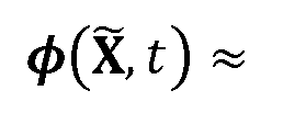
- the material deformation may be characterized in terms of the flow map ⁇ , which maps points in the original configuration of the material X to points in the time t configuration x as The Jacobian of this mapping may be referred
- deformation gradient which represents the local deformation of the material. That is, the deformation gradient yields the best local linear approximation to the mapping:
- Codimensional deformation may be expressed via components of F.
- Material directions D x , D 2 , D 3 are defined at point X.
- D x and D 2 are tangent to the initial configuration of the surface and D 3 is normal to the surface.
- D x is tangent to the curve and D 2 and D 3 are orthogonal to D x .
- deformation in the manifold may be expressed via di; for surfaces, deformation in the manifold may be expressed via d x and d 2 .
- the remaining d ⁇ represents the deformation of material normal to the manifold.
- the model can account for deformation in the manifold, deformation normal to the manifold and shearing of material relative to the manifold, in terms of the d ⁇ and their relation to one another.
- D 3 is normal to the initial surface, d 3 will not be normal when there is a shearing motion relative to the manifold.
- FIG. 8 illustrates modeling of a curve in a 2-dimensional (2D) space.
- the plastic part F p may represent deformation history that has been lost and may no longer be penalized elastically.
- the elastic part F £ may remain and may be penalized elastically.
- a hyperelastic potential energy density may be used, which increases with increasing deformation in F £ .
- frictional contact may be modeled with elastoplasticity.
- the modeling of the elastic surface or curve may consider contact to occur in the direction orthogonal to the elastic surface or curve. Therefore, the plasticity may modify the codimensional components of the deformation.
- the mechanical response to deformations in the manifold may be purely elastic, which places an anisotropic constraint on the multiplicative decomposition.
- the plasticity model may satisfy (equivalently To guarantee that the
- the model may additionally satisfy
- plasticity may be allowed just to affect the components of the deformation that provide compression, extension and shearing in directions normal to the manifold.
- the disclosed approach may use a model that is hyperelastic in F £ , where the elastic potential energy density increases with deformation of the elastic part of the deformation gradient.
- the Cauchy stress in the material may be
- the elastic energy density for penalizing non-rigid F £ is the elastic energy density for penalizing non-rigid F £ .
- the elastic energy density for penalizing non-rigid F £ is the elastic energy density for penalizing non-rigid F £ .
- the elastic energy density may serve at least two purposes.
- the elastic energy density may express the resistance to deformations that change the shape of the surface or curve manifold.
- the elastic energy density may define the resistance to contact and frictional sliding. In the case of codimensional elasticity, the resistance is due to deformations normal to the manifold.
- the anisotropic energy density may take this dual nature into account.
- the elastic potential may be invariant under world space rotations.
- one choice may be given by orthogonalizing the vectors the elastically deformed material directions, with the Gram-Schmidt process to
- model may define This is similar to the isotropic case where the additional material frame invariance allows a model to choose u t and v t such that and
- another common stress measure may be the first Piola- Kirchhoff stress, defined as and related to ⁇ with . If F £ D is
- T and D are operators on matrices that keep upper triangular part
- Elastic curves may be modeled with rotational material symmetry around the fiber direction D x .
- the material directions D 2 and D 3 may be regarded as essentially arbitrary, and any choices which are mutually orthogonal with D x may give the same potential.
- this material symmetry may be decomposed into a composition of three deformations, where the first (R x ) is a stretching of the fibers, the second (R 2 ) is a shearing of the fibers and the third (R 3 ) is a deformation of the cross section of the fibers:
- the elastic potential for curves may be expressed as a sum of 3 terms
- the first term penalizes
- the second term penalizes shearing along the
- the third term /i(R 3 ) may be a form of a two dimensional elastic potential, since it naturally enforces the frictional contact (when combined with appropriate plasticity law). That is,
- e 1 and e 2 are the logarithms of the nontrivial singular values of R 3 .
- the surface may be assumed as being isotropic, e.g., the potential is invariant under rotation of the material directions D-, ⁇ and D 2 .
- R R 3 R 2 R X is decomposed into a composition of three deformations.
- the first (R x ) is an in- plane deformation of the surface.
- the second (R 2 ) is a shearing of surface normal.
- the third (R 3 ) is a compression or stretching of the surface normal:
- the energy may be expressed as a sum of three terms,
- the first term (R 3 ) may penalize compression of the material in the normal direction, since the surface may be mostly surrounded by empty space which can expand freely:
- the second term may be a form of to penalize shearing of the
- the third term hiR ⁇ may use a two dimensional version of a fixed corotated potential to penalize deformation of the surface.
- any in-plane energy may be used, with no change except to the stress and stress derivatives.
- the frictional force ff may be smaller than a constant c F (the coefficient of friction) times the normal force In a continuum view, at a given
- the traction vector t represents the local force per area that the material on one side of the plane with normal n exerts on the other side.
- the traction may have normal and shearing components
- s(n, ⁇ ) is an arbitrary vector in the plane with normal n, and ⁇ indicates its direction in the plane.
- contact may be assumed to happen in all directions.
- the model considers the directions orthogonal to the manifold to be in frictional contact. Together with the choice of elastic potential, this results in a less restrictive constraint that does not affect elastic deformation in the manifold.
- the disclosed approach may include MPM discretization, which translates from the theoretical continuum equations into a computation procedure for codimensional elasticity with contact.
- PIC and MPM may be hybrid particle/grid methods.
- the particles represent discrete samples of the continuous material and the grid is a helper for computing their physical interactions.
- the particles may be rendered as individual grains and the grid update, whose essential features are inherited from the continuum, which can be seen as a means for processing their frictional contact interactions.
- the continuum samples may be modeled as coherent surface or curve meshes, rather than as unstructured particles, which is different from other MPM approaches.
- the disclosed MPM discretization may model self-collision and its ramifications in the grid momentum updates, as well as the associated elasticity and plasticity updates.
- the discretization procedure may include:
- the Lagrangian particle state may be the primary representation of material for MPM.
- Particles can be classified as: (i) traditional MPM particles, (ii) Lagrangian mesh vertex particles, or (Hi) Lagrangian mesh element quadrature particles (e.g., see FIG. 11).
- Type (ii) particles may be used to track the in-manifold deformation of the elements.
- Type (Hi) particles may be used to track to the codimensional deformation in an updated Lagrangian manner.
- the model stores the particle positions velocities initial mass m p .
- D p is not stored for particles of type (i) and (ii). is not stored for particles of type (ii).
- the mass is set as is set
- the notation / ( , I m , I m may be used to represent the sets of particle indices of types (i),(ii) and (Hi) respectively.
- the particle is in one of /( ; /(") or depending on its type.
- the particle mass and momentum may be transferred to the grid using, e.g., APIC.
- Each particle p and grid node i is associated with a weight
- ⁇ ⁇ is the location of the grid node and N(x) are linear, quadratic or cubic
- node i is a sum of the contributions from particles
- each particle also stores matrix to define an affine velocity local to the
- p is generated for grid momentum and then is divided by the grid mass to generate the grid velocity as
- the Rigid Particle-in-Cell may be treated as a reduced APIC scheme that damps out stretching and shearing motions while conserving rigid velocity modes. APIC degrades to RPIC if just the skew symmetric part of is kept.
- the model may stably introduce damping to the system by scaling
- v G [0,1] is the damping coefficient. This allows controlling the damping on stretching and shearing without damping local or global rigid motions.
- any value of v may be chosen depending on how energetic a simulation is.
- the damping scheme may damp non-rigid motion in a stable way without introducing any additional time step restriction. For example, the damping scheme may work with explicit symplectic Euler time stepping.
- the continuum samples may be treated as coherent surfaces or curves, rather than as unstructured particles.
- the treatment may be applied to, e.g., elastic volumes and surfaces (without self-collision).
- the Eulerian MPM update of the deformation gradient may be abandoned, and the mesh connectivity may be used to compute the manifold components of the deformation gradient.
- This approach may also be applied to triangulated surfaces and segmented curves. This allows for a Lagrangian update of the deformation gradient that does not suffer from the numerical plasticity or fracture of the Eulerian update.
- the approach allows for coupling of Lagrangian elastic meshes with MPM materials. However, self-contact with codimensional meshes may not be well resolved.
- the disclosed approach further introduces an Eulerian deformation of the grid, to obtain the full rank deformation gradient.
- the disclosed approach allows for penalizing self-contact, while still preventing numerical plasticity and fracture.
- a comparison of the approaches with or without Eulerian deformation of the grid is shown in FIG. 10.
- the deformation gradient may be updated in terms of the motion of the grid over a time step.
- the motion of the grid may be described in terms of Xi , the Eulerian grid nodes at the beginning of the time step and x t their location after a grid update.
- the grid momentum update may be treated in terms of the motion that it may cause on the grid. In particular, this allows defining the elastic grid forces through a differentiation of a potential.
- the use of incremental grid node motion is referred to as an updated Lagrangian view. In other words, the motion of the grid is treated as Lagrangian, albeit from the grid configuration at time t n , instead of the rest configuration.
- the locations are updated to denote the vector of all moved grid positions X; and velocities respectively, the deformation gradient update on particle p may be defined in terms of
- the elastic deformation gradient may be updated as: where assuming no initial deformation.
- the deformation gradient may not be stored, so elastic deformation gradient may not be updated.
- a Lagrangian mesh element quadrature particle e.g., type (/ ' /)
- the deformed edge vectors are interpolated from the deformed grid node positions
- the ⁇ directions tangent to the manifold may not include superscript E since they may not experience plasticity.
- the remaining 3 — ⁇ directions may be of unit length and normal to the manifold, and may be evolved as in MPM via
- the update of the grid node momentum (e.g., velocities since the grid node masses do not change in the update) may be described as:
- the hat in distinguishes the update from the velocities that may be transferred to the
- the grid momentum update may be expressed as: where f is the elastic force, g is the gravitational acceleration and for symplectic Euler
- the elastic force f may be defined in terms of the elastic potential energy. Given elastic energy density ⁇ , the total potential may be computed as over material
- [00109] may be a third order tensor, and may not depend on because is linear in
- the tensor allows splitting the computation into three parts.
- the first part corresponds to MPM particles and the force is - y expressing F using a material space coordinate frame which is aligned with the element
- the first ⁇ columns of F may be assumed to correspond to in-manifold deformation.
- the first ⁇ columns of correspond to the stress response inside the manifold and these terms can be computed by first computing forces on Lagrangian mesh vertex particles (type (/ ' / ' )) and then transferring them to the grid. Denoting these vertex forces with their corresponding contribution to grid node forces may be computed as The last 3— ⁇ columns
- the system when using backward Euler, the system may be modeled by utilizing the Hessian of ⁇ with respect to and ignoring the effects of plasticity during the process.
- the action of this Hessian on an arbitrary increment Su may be expressed as where implicit summation
- GMRES generalized minimal residual method
- MINRES minimal residual method
- the return mapping may be a discrete version of the yield condition and flow rule.
- the return mapping may be a form of a projection, which enforces the yield condition on the stress, with the direction of the flow rule, defining the direction of the projection.
- the return mapping may be applied after the deformation gradient update so that the updated stress may satisfy the yield condition.
- the QR-decomposition may be generated as is projected from to satisfy the yield condition, before constructing
- the stress satisfies for every normal n to the curve
- + c F n T t ⁇ Ois satisfied, where n q 3 .
- the traction may be expressed as
- uniform scaling may be applied:
- the magnitude of the tangential traction may change, but the direction may not change, corresponding to the uniform scaling.
- the return mapping may be independent of the choice of in-plane energy /i(Ri). E.g., the in-plane surface energy may be used from instead.
- FIG. 16 illustrates the return mapping of a 2D curve. is unchanged.
- each shaded region corresponds to the feasible state of the deformed material normal and is determined by the yield function.
- the right figure shows the same yield surface in r 12 r22 space.
- the tip of the yield surface corresponds to the world space manifold normal and is usually different from d 2 .
- the Return mapping may take a trial strain and results in the
- the particle corresponding to is inside the yield surface and exhibits an elastic response.
- the particle corresponding to is under compression but experiences more shear than friction allows.
- Such a configuration is projected to the yield surface along the direction that avoids normal component change.
- the particle corresponding to is experiencing tension and is projected to the tip of the yield surface.
- the corresponding stress is zero, allowing materials to separate freely.
- the particle corresponding to is inverted from the original side of material (due to discrete numerical step).
- the shearing may be disabled by nullifying the r 22 component, and relying on elasticity to penalize such configuration.
- Fibrous materials may have anisotropic friction.
- hair may be smoother along the fiber direction than perpendicular to the fiber direction.
- an anisotropic friction rule may be used, which is stricter and easier to apply.
- mapping may be described in terms of the logarithms of
- the model may choose to make
- the model constructs .
- the model determines if the condition for shearing tangent to the fibers is satisfied. If the
- Table 1 lists parameter choices for some simulation examples.
- Table 2 lists runtime performance results for some simulation examples. In some embodiments, some simulations may be run on Intel Xeon E5-2690 V2 with 19 threads.
- Element # denotes number of triangles (for surfaces), number of segments (for curves) or the total count (for coupling simulations).
- Memory usage is measured in the end of the first frame. At here means maximum allowed time step.
- the actual running At is adaptive and may be restricted by Courant-Friedrichs-Lewy (CFL) condition when the particle velocities are high.
- CFL number equals to 0.3, e.g., particles are not allowed to move further than 0.3 ⁇ in a time step.
- FIG. 12 illustrates a simulation of 2D curves with different friction coefficients dropping on a block. Internal friction may be naturally controlled via adjusting c F .
- the surface elastoplasticity model may simulate cloth triangulated surfaces in various scenarios involving numerous self-collisions (see, e.g., FIG. 1, FIG. 3, FIG. 4 and FIG. 14).
- the elastoplasticity model can resolve frictional contacts with a modest computational cost.
- the run time may not grow with the number of colliding primitives.
- the fiber elastoplasticity may be simulated with yarn level simulation of knitted fabric.
- multiple threads per yarn may be simulated.
- a mesh model may be used to simulate different examples including, e.g., dropping a sweater (FIG. 7), a jumping character wearing a poncho (FIG. 17), twisting a knitted cloth with a cylinder (FIG. 5), and hitting a knitted cloth curtain with a ball (FIG. 14).
- the fiber model may also be suitable for simulating hair (FIG. 13), shag carpet (FIG. 2) and other fibrous materials (FIG. 6).
- each strand may be simulated.
- the disclosed method scales well regardless of the complexity of segment contacts. RPIC damping may be used for stabilizing the simulations under large timesteps.
- FIG. 1 and FIG. 9 illustrates a sand column with 7 millions particles coupled with a piece of cloth.
- FIG. 19 illustrates a cloth curtain getting hit by a ball while interacting with sand and/or goo.
- FIG. 18 illustrates dripping viscous green slime into an elastic bear geometry.
- a relatively high collision stiffness (k) may be set on the cloth to prevent sand from sticking to it.
- the result of disclosed method is compared with other MPM approaches by simulating multiple curves dropping onto a block (see FIG. 10).
- Other meshless MPM causes numerical fracture of the material.
- the other method may just model the manifold stress response, resulting in unnatural clumping and numerical cohesion of curves.
- the disclosed method adopts a full elastoplasticity model, achieves natural and realistic dynamics, and exhibits a smooth frictional sliding appearance, without excessive frictional effects.
- the disclosed method may use a regular grid to resolve material interactions.
- the apparent thickness of the surface and/or curve may depend on the grid resolution and on the repulsion energy model.
- the disclosed method may be modified to reduce or eliminate artifacts when if the grid resolution is large. For a large grid resolution, the artifacts may manifest as numerical separation where particles tend to stay separated by an amount about half a grid cell width or numerical stickiness. Thus, the motion of the grid may be accurate to resolve the proper behavior. Therefore the method may simulate frictionless materials and control the apparent thickness independent of the grid.
- the disclosed method is suitable for situation where the size of the surface or curve elements is at most the size of the grid spacing.
- the disclosed method may be modified to reduce or eliminate persistent wrinkles, which may manifest when a mesh is fine compared to the grid.
- the disclosed method may be modified to reduce or eliminate self-penetration, which may manifest when a mesh is coarse compared to the grid because the material coverage is not resolved well enough on the grid. When penetration accidentally happens (due to At being too big), it may be resolved because elasticity may penalize that inverted collision direction.
- the disclosed method may prevent the self- penetration by enforcing the CFL condition when choosing At. The disclosed method may use small time steps and increase overall run time.
- the disclosed method when transferring from particles to grid, may determine local neighbor information.
- the penalty on compression in the normal direction may be treated as repulsion springs.
- no fail-safe is used to prevent self-penetration when the repulsions fail.
- the disclosed method may have smaller time steps for high grid resolution simulation, without fail-safes.
- the disclosed method performs well for high resolution examples. E.g., for the cloth curtain example (FIG. 14), the disclosed method may achieve computation times of, e.g., 2 minutes per frame on average for, e.g., 1.8 million triangles.
- the disclosed method tends to scale as well as the particle-grid transfers.
- the process may be performed in parallel over multiple CPU threads.
- performance gains may be achieved with a GPU implementation.
- the continuum based bending model may be used.
- any that satisfy may be upper triangular. Specifically, it may be shown that given arbitrary upper triangular, 3 ⁇ such that
- A may be ⁇ written in the Q basis.
- the upper triangular part of A may be contstructed with , then
- the process may choose to be the dilational part of the Kirchoff stress from the 2 x 2 Stvk Hencky Drucker-Prager.
- Mohr friction criteria may lead to the following maximization: maximization of over all possible n that is perpendicular to
- Lagrangian multiplier may solve the maximization and lead to the maximum
- the yield surface may be The return
- mapping is then simply a scaling on r so that the yield criteria is satisfied.
- Surface may be similar to curve in the framework. With the codimensional discretization, the triangle may be mapped back to x-y plane. If the input 3D triangle at rest is the method may define This forms an imaginary whose QR decomposition leads to the rotation from x-y plane of this triangle as well as the top part of being the 2 X 2 version D m . The third column of is the rotated D 3 where
- the full F may be constructed as:
- the method performs thin QR decomposition: where may be 2 x 2 upper.
- This tensor may be denoted with A
- triangular part of A may be constructed with then symmetry of A is used.
- r3 represents the deformation of D 3 . because is the length change
- Shearing may also penalize length change.
- Mohr friction criteria leads to the following maximization: Maximization of over all possible n that is perpendicular to the manifold plane, with all d perpendicular to n and has unit length. In other words, is maximized over all possible n that is perpendicular to the
- n perpendicular to manifold plane means for some k (unit
- the return mapping causes r to be zero.
- the max may choose The return mapping is setting r to be 0. Otherwise, r may be scaled to satisfy
- 2D derivation may follow 3D curve derivation: have the
- This tensor may be denoted with
- A may be ⁇ written in the Q basis.
- the energy choice may be any one of [00179]
- Mohr friction criteria may lead to the following maximization: maximization of over all possible n that is perpendicular to
- scale r 12 may be scaled to satisfy
- the undeformed segment or triangle may be treated as being aligned with the x-axis or xy-plane respectively.
- the initial F may no longer be I, but rather the rotation which maps the axis aligned element to its initial position in space. This is may not be an issue as the elastic energy density ⁇ may be world space rotation invariant. However, this allows assuming that Drete is block diagonal of the form for segments and
- FIG. 20 is a high-level block diagram illustrating an example of a hardware architecture of a computing device 1100 that may perform various processes as disclosed, according various embodiments of the present disclosure.
- the computing device 1100 may execute some or all of the processor executable process operations or procedures described herein.
- the computing device 1100 includes a processor subsystem that includes one or more processors 1102.
- Processor 1102 may be or may include, one or more programmable general-purpose or special-purpose microprocessors, digital signal processors (DSPs), programmable controllers, application specific integrated circuits (ASICs), programmable logic devices (PLDs), or the like, or a combination of such hardware based devices.
- DSPs digital signal processors
- ASICs application specific integrated circuits
- PLDs programmable logic devices
- the computing device 1100 can further include a memory 1104, a network adapter 1110, a cluster access adapter 1112 and a storage adapter 1114, all interconnected by an interconnect 1108.
- Interconnect 1108 may include, for example, a system bus, a Peripheral Component Interconnect (PCI) bus, a HyperTransport or industry standard architecture (ISA) bus, a small computer system interface (SCSI) bus, a universal serial bus (USB), or an Institute of Electrical and Electronics Engineers (IEEE) standard 1394 bus (sometimes referred to as "Firewire”) or any other data communication system.
- PCI Peripheral Component Interconnect
- ISA HyperTransport or industry standard architecture
- SCSI small computer system interface
- USB universal serial bus
- IEEE Institute of Electrical and Electronics Engineers
- the cluster access adapter 1112 includes one or more ports adapted to couple the computing device 1100 to other devices.
- Ethernet can be used as the clustering protocol and interconnect media, although other types of protocols and interconnects may be utilized within the cluster architecture described herein.
- the computing device 1100 can be embodied as a single- or multi-processor storage system executing a storage operating system 1106 that can implement a high-level module, e.g., a storage manager, to logically organize the information as a hierarchical structure of named directories and files at the storage devices.
- the computing device 1100 can further include graphical processing unit(s) for graphical processing tasks or processing non-graphical tasks in parallel.
- the memory 1104 can comprise storage locations that are addressable by the processor(s) 1102 and adapters 1110, 1112, and 1114 for storing processor executable code and data structures.
- the processor 1102 and adapters 1110, 1112, and 1114 may, in turn, comprise processing elements and/or logic circuitry configured to execute the software code and manipulate the data structures.
- the network adapter 1110 can include multiple ports to couple the computing device 1100 to one or more clients over point-to-point links, wide area networks, virtual private networks implemented over a public network (e.g., the Internet) or a shared local area network.
- the network adapter 1110 thus can include the mechanical, electrical and signaling circuitry included to connect the computing device 1100 to the network.
- the network can be embodied as an Ethernet network or a Fibre Channel (FC) network.
- a client can communicate with the computing device over the network by exchanging discrete frames or packets of data according to pre-defined protocols, e.g., TCP/IP.
- the storage adapter 1114 can cooperate with the storage operating system 1106 to access information requested by a client.
- the information may be stored on any type of attached array of writable storage media, e.g., magnetic disk or tape, optical disk (e.g., CD- ROM or DVD), flash memory, solid-state disk (SSD), electronic random access memory (RAM), micro-electro mechanical and/or any other similar media adapted to store information, including data and parity information.
- the storage adapter 1114 can include multiple ports having input/output (I/O) interface circuitry that couples to the disks over an I/O interconnect arrangement, e.g., a conventional high-performance, Fibre Channel (FC) link topology.
- the cluster adapter 1112 and the storage adapter 1114 can be implemented as one adaptor configured to connect to a switching fabric, e.g., a storage network switch, in order to communicate with other devices and the mass storage devices.
- Amounts, ratios, and other numerical values are sometimes presented herein in a range format. It is to be understood that such range format is used for convenience and brevity and should be understood flexibly to include numerical values explicitly specified as limits of a range, but also to include all individual numerical values or sub-ranges encompassed within that range as if each numerical value and sub-range is explicitly specified.
Landscapes
- Engineering & Computer Science (AREA)
- Physics & Mathematics (AREA)
- Theoretical Computer Science (AREA)
- General Physics & Mathematics (AREA)
- Computer Graphics (AREA)
- Computer Hardware Design (AREA)
- Evolutionary Computation (AREA)
- Geometry (AREA)
- General Engineering & Computer Science (AREA)
- Management, Administration, Business Operations System, And Electronic Commerce (AREA)
- Processing Or Creating Images (AREA)
Abstract
At least some embodiments of the present disclosure relate to a method of visualizing objects having frictional contact. The method includes transferring masses and momentums of a plurality of particles of an object to a grid including a plurality of grid nodes; updating momentums of the grid nodes based on the transferred masses and momentums of the particles; transferring the updated momentums of the grid nodes to the particles of the object; updating positions of the particles and deformation gradients of the particles based on the updated momentums of the grid nodes; projecting the deformation gradients for plasticity of the object; updating elastic components and plastic components of the object; and outputting a visualization of the object based on the positions of the particles of the object.
Description
COMPUTERIZED RENDERING OF OBJECTS HAVING ANISOTROPIC ELASTOPLASTICITY FOR CODIMENSIONAL FRICTIONAL CONTACT
CROSS-REFERENCE TO RELATED APPLICATION
[0001] This application claims the benefit of and priority to U.S. Provisional Patent Application No. 62/507,740, filed May 17, 2017, which is incorporated herein by reference in its entirety.
STATEMENT REGARDING FEDERALLY SPONSORED RESEARCH OR
DEVELOPMENT
[0002] This invention was made with government support under W81XWH-15-1-0147 awarded by the U.S. Army, Medical Research and Materiel Command. The government has certain rights in the invention.
TECHNICAL FIELD
[0003] The present disclosure relates to a physically based animation, and more particularly to a computerized simulation of 3 -dimensional (3D) objects having elastic surfaces or curves.
BACKGROUND
[0004] Physically based animation is used to simulate physically plausible behaviors of objects. The techniques of physically based animation are particularly concerned with physical plausibility, numerical stability, and visual appeal of the objects being simulated or animated. The techniques of physically based animation include simulations of, e.g., rigid bodies (e.g., metal objects, rocks), soft bodies (e.g., muscle, fat, hair, vegetation, clothing, fabric), fluid (e.g., water), particles (e.g., smoke, fire, moving water, cloud, snow, dust, stars), as well simulations of complex behaviors of various objects (e.g., humans, animals, plants, clothing, etc.) and interactions between objects.
BRIEF DESCRIPTION OF THE DRAWINGS
[0005] Aspects of the present disclosure are best understood from the following detailed description when read with the accompanying drawings. It is noted that various features may
not be drawn to scale, and the dimensions of the various features may be arbitrarily increased or reduced for clarity of discussion.
[0006] FIG. 1 illustrates a simulation of a sand column being coupled with a piece of cloth. The left figure illustrates three pieces of cloth with around 1.4 million (M) triangles pushed back and forth by a sphere, revealing intricate folds and contact. The right figure illustrates 7M (millions) colored sand grains coupled with elastic cloth, exhibiting beautiful flow patterns.
[0007] FIG. 2 illustrates a simulation of a shag carpet with 1M particles that is pushed by a sphere and folds back, showing detailed folds.
[0008] FIG. 3 illustrates a simulation of a piece of cloth interacting with a ball, where the piece of cloth with 2M triangles falls onto a rotating sphere, and low friction on the ground and high friction on the sphere causes detailed wrinkles and folds.
[0009] FIG. 4 illustrates a simulation of a piece of cloth being twisted, where the piece of cloth with 1.14M triangles is twisted by a cylinder. The simulation may run at 1.3 minutes per frame on average.
[0010] FIG. 5 illustrates a simulation of twisting a knitted cloth with a cylinder. The method handles detailed contacts between individual yarn threads under tension as well as macroscopic collision between yarns as demonstrated by this knitted cloth being twisted. Complex per-yarn motion is well resolved through elastoplasticity.
[0011] FIG. 6 illustrates a simulation of tearing apart a fibrous material. The method may capture many intricate features of tearing apart the fibrous material comprising, e.g., 2.15M particles.
[0012] FIG. 7 illustrates a simulation of dropping a knit sweater, where the sweater is dropped onto a rising sphere, stretched and then folded on the ground. The simulation may take 13 seconds per frame.
[0013] FIG. 8 illustrates a simulation of a curve in a 2-dimensional (2D) space. The left figure shows F being decomposed into Fp, a forgotten sliding and separation, and FE the remembered stretching, collision and shearing. The right figure shows that FE deforms Di and
D2 into di and d2 .
[0014] FIG. 9 illustrates a simulation of a two-way coupling between 7M sand grains and a piece of elastic cloth.
[0015] FIG. 10 illustrates effects of different choices of deformation gradient discretization as well as the effect of plasticity in a fiber piling example, (a) shows MPM deformation gradient; (b) shows the codimensional Lagrangian deformation gradient; (c) shows the disclosed model without plasticity; (d) shows the disclosed full elastoplasticity model.
[0016] FIG. 11 illustrates a simulation of particles of different classifications, including Material Point Method (MPM) particles, Lagrangian mesh vertex particles, and Lagrangian mesh element quadrature particles.
[0017] FIG. 12 illustrates effects of increasing friction in a 2-dimensional piling example. Friction increases from left to right.
[0018] FIG. 13 illustrates a simulation of a hair tube with 2655 strands that is dropped onto another tube of hairs, showing detailed dynamics due to fiictional contact between hairs. The simulation may run at, e.g., 11 seconds per frame.
[0019] FIG. 14 illustrates a simulation of a knitted curtain being pushed by a sphere and folding back.
[0020] FIG. 15 illustrates a simulation of stretching, twisting and releasing a knitted cloth from different directions, which demonstrates handling yarn level anisotropic characteristics.
[0021] FIG. 16 illustrates a simulation of a return mapping for a 2D curve.
[0022] FIG. 17 illustrates a simulation of a character wearing a knitted poncho performing a jumping motion. The fiber elastoplasticity model captures detailed frictional contact behavior at the yarn level with multiple fiber threads per yarn. The simulation may run at, e.g., 1 minute per frame on average.
[0023] FIG. 18 illustrates a simulation of a two-way coupling of solids and fluids, as demonstrated with slime and a cloth bear.
[0024] FIG. 19 illustrates a simulation of a cloth curtain being hit by a ball and coupling with
sand and a simulation of a cloth curtain being hit by a ball and coupling with goo.
[0025] FIG. 20 is a high-level block diagram illustrating an example of a hardware architecture of a computing device that may perform various processes as disclosed.
DETAILED DESCRIPTION
[0026] Common reference numerals are used throughout the drawings and the detailed description to indicate the same or similar components. Embodiments of the present disclosure will be readily understood from the following detailed description taken in conjunction with the accompanying drawings.
[0027] Various embodiments of the present disclosure are discussed in detail below. It should be appreciated, however, that the embodiments set forth many applicable concepts that can be embodied in a wide variety of specific contexts. It is to be understood that the following disclosure provides many different embodiments or examples of implementing different features of various embodiments. Specific examples of components and arrangements are described below for purposes of discussion. These are, of course, merely examples and are not intended to be limiting.
[0028] Embodiments, or examples, illustrated in the drawings, are disclosed below using specific language. It will nevertheless be understood that the embodiments and examples are not intended to be limiting. Any alterations and modifications of the disclosed embodiments, and any further applications of the principles disclosed in this document, as would normally occur to one of ordinary skill in the pertinent art, fall within the scope of this disclosure.
[0029] In addition, the present disclosure may repeat reference numerals and/or letters in the various examples. This repetition is for the purpose of simplicity and clarity and does not in itself dictate a relationship between the various embodiments and/or configurations discussed.
[0030] According to at least some embodiments of the present disclosure, computerized simulation method of elastic surface or curve involves a hybrid approach combining a Lagrangian approach and an Eulerian approach. The computerized simulation method can be used for applications such as computer-generated imagery for rendering 3 -dimensional (3D) objects in graphics, animations, videos, movies, video games, etc.
[0031] In some embodiments, an elastic surface or curve simulation method involves, e.g., a Lagrangian approach and includes three components: time integration, collision detection and collision response. The Lagrangian approach allows for tracking of the codimensional manifold. However, collision may be detected and resolved separately. In some embodiments, an elastic surface or curve simulation method involves, e.g., an Eulerian method, for which the collision processing is automatic. The Eulerian method may be effective for volumetric objects. However, advection of a codimensional manifold may be relatively inaccurate. The term "codimensional" refers to objects of submanifolds (e.g., less dimensions) in a space of manifolds (e.g., more dimensions). For example, a hair line (1 dimension) or a piece of paper (2 dimensions) can be a codimensional object simulated and visualized in a 3-dimentionsal space.
[0032] In some embodiments, a hybrid approach, combining a Lagrangian approach and an Eulerian approach, defines the collision response with an elastoplastic constitutive model. For example, an anisotropic hyperelastic constitutive model separately characterizes the collision response to manifold strain as well as shearing and compression in the directions orthogonal to the manifold. The model is discretized with a Material Point Method (MPM) and a codimensional Lagrangian/Eulerian update of deformation gradient. The hybrid approach can simulate a large number of collisions in a short time frame. For example, in some embodiments, collision intensive scenarios with millions of degrees of freedom may take a few minutes per frame (or less). In some embodiments, examples of collision intensive scenarios with up to one million degrees of freedom may run in less than thirty seconds per frame (or less).
[0033] 1. INTRODUCTION
[0034] Computer graphics may involve physically based animation of elastic surfaces and curves. For example, elastic surfaces and curves can include, e.g., layers of clothing in a virtual garment, individual strands in a head of hair, or yarns in a knit garment. Realistic simulation of collision and contact phenomena of these materials allows for richness and realism provided by physics based simulation. However, the thin nature of these materials may make collision detection and resolution challenging. The time-consuming process of collision detection and resolution of these materials can be the bottleneck in modern visual effects.
[0035] According to at least some embodiments of the present disclosure, an approach for codimensional elasticity that uses a hybrid Lagrangian/Eulerian Material Point Method (MPM) discretization is disclosed for modeling frictional contact of these granular materials with a continuum view. The elastoplastic description of the disclosed approach characterizes collision and/or contact response in the continuum and does not necessarily include separate post-processing (although post-processing is also feasible).
[0036] In some embodiments, codimensional elastic objects are naturally represented with a Lagrangian mesh. With the Lagrangian mesh model, individual particles are tracked and mesh polygons or segments are used to approximate the spatial derivatives of the material deformation mapping (also referred to as the deformation gradient). The mechanics of elasticity are naturally discretized with this Lagrangian view. However, additional modeling may be used to model the effects of self and external contact since these phenomena may cause interactions between distant regions in the mesh. For example, mesh facets such as points and triangles or segment pairs may not pass through one another over a time step. These constraints may be satisfied by some means external to the elasticity modeling. This can be done in number of ways including, e.g., repulsion penalties, impulsive change in momenta, and/or linear complimentary formulations of the constrained dynamics.
[0037] In some embodiments, in an Eulerian view, discrete samples of the solution are computed on a stationary background grid as material advects through the domain. While Lagrangian methods may involve two different components of the computation procedure: elasticity modeling and collision and/or contact resolution, Eulerian methods typically do not. The constitutive behavior of contact is expressed as that of the material itself. For example, for free-surface incompressible flow, no self-collision model is imposed beyond the velocity divergence condition specified to enforce incompressibility. In some embodiments, Eulerian methods may be used for collision and contact treatment for elastic materials. For elastic objects, accurate treatment of advection may be used to preserve an accurate rest state of the material, e.g. treatment for volumetric objects. However, Eulerian methods may face challenges for codimensional elasticity.
[0038] The disclosed hybrid approach combines the benefits of the Lagrangian and Eulerian approaches. For example, Particle-In-Cell (PIC) approaches like FLIP and MPM may combine a Lagrangian form of advection with a regular grid momentum update. In some
embodiments, contact modeling may be simplified with Lagrangian methods, or the advection accuracy may be improved with Eulenan methods. For example, FLIP and Eulerian incompressibility may be used to efficiently model self-collision for hair. In a hybrid approach, Lagrangian hair velocities may be smoothed on an Eulerian grid. A hybrid approach may define interaction penalties and constraints for Lagrangian objects after mapping mass, momentum and density to an Eulerian grid. MPM has some similarities to this approach and may allow for the simulation of a wide range of elastoplastic materials in contact without a separate model for collision. For example, volumetric hyperelastic objects in contact with MPM may be simulated. Frictional contact for sand, for example, may be modeled with a hybrid discretization of an appropriate plastic flow.
[0039] According to at least some embodiments of the present disclosure, a hybrid approach may combine Lagrangian and Eulerian MPM methods, for modeling contact and collision via elastoplasticity of granular materials, and may be used to model volumetric objects. In some embodiments, MPM may update the deformation gradient on each particle independently with an Eulerian view. However, this may lead to numerical plasticity and failure. While these phenomena may useful for simulating elastoplasticity with failure, it is desirable to avoid these phenomena for simulating hyperelastic objects. To prevent numerical plasticity and failure, the disclosed hybrid approach tracks the deformation of codimensional elastic objects in a Lagrangian way.
[0040] However, in some embodiments, some approaches allowing for self-collision with volumetric objects may not be suitable for modeling codimensional objects. For non- volumetric objects such as codimensional objects, the Lagrangian update of deformation may track components in the manifold, but may not capture deformation in the orthogonal directions. It may be the elastic response to deformation in these directions that allows for frictional contact with volumetric objects in MPM simulations. The disclosed hybrid approach remedies the issue by updating the orthogonal components of the deformation gradient, e.g., in a standard MPM way.
[0041] Furthermore, in some embodiments, while relying on the elastic response alone may be sufficient for self-collision simulation with volumetric objects, it may lead to artificial cohesion (stickiness) and excessive friction for codimensional elasticity. The disclosed hybrid approach remedies this using a plastic flow that enforces a Coulomb friction inequality
between shear and normal stresses in the directions orthogonal to the frictional surface or curve. The disclosed approach prevents plasticity in the codimensional manifold, which may be purely elastic. The disclosed approach defines the elasticity in an anisotropic way so that the response in the surface or curve cleanly relates to the response in the orthogonal directions.
[0042] In some embodiments, the disclosed approach is computationally efficient, at least partially due to the simplicity of handling contact and collision through the constitutive modeling. Furthermore, the disclosed approach inherently and naturally allows for coupling with multiple materials. For example, the disclosed approach can simulate a range of coupled elastic surfaces and curves, fluids and granular materials with, e.g., millions of degrees of freedom in, e.g., a few minutes per frame. The disclosed approach may involve both implicit and explicit versions of the grid based momentum update in MPM. For explicit time stepping, the disclosed approach uses a damping model that may not penalize rigid motions and may not impact the time step restriction.
[0043] In some embodiments, the disclosed approach use elasticity models that cleanly relate the elastic response in the surface or curve to the response in the orthogonal directions. Anisotropic plasticity models are used to characterize frictional contact with elastic surfaces and curves. A return mapping procedure is used to temporally discretize the plastic flow. A hybrid version of Lagrangian and Eulerian MPM discretization is used for updating the deformation gradient. The disclose approach involves an explicit damping model that may not penalize rigid modes.
[0044] 2. RELEVANT TECHNIQUES
[0045] 2.1 Simulation of Clothing
[0046] In some embodiments, clothing simulation may use dynamically defined stiff springs that prevent cloth-cloth penetration and apply an implicit integration scheme for efficiency. A semi-implicit treatment may be used to efficiently handle buckling instabilities. Collisions for point/triangle and edge/edge pairs in the mesh may be processed via impulsive response. Asynchronous variational integration may be combined with kinetic data structures. Collision resolution may be processed with barrier potentials which efficiently approximate with nested families of quadratic potentials. An implicit treatment of complimentary collision constraints
and a solver for large mixed linear complementarity problems may be used. Implicit time stepping for cloth may be performed efficiently via optimization with auxiliary variables representing strain.
[0047] 2.2 Simulation of Yarn and Knits
[0048] Elastic curves representing individual yarns may be used to create knit garments. Infrequently updated locally co-rotated linear approximations of the barrier potential may be used to provide a speed up of, e.g., fivefold. Warp/weft intersections may be resolved with a point that connects the two curves.
[0049] 2.3 Simulation of Hair
[0050] In some embodiments, hair may be modeled with various elasticity models per strand. In some other embodiments, hair may also be modeled as inextensible. For example, Kirchhoff elastic rod models may be used, which naturally enforce inextensibility. Frictional effects may be included in the hair modeling. In some embodiments, impulse-based collision models for elastic rods may lead to instabilities via excitation of stretching modes, and an adaptively nonlinear model for collision may lead to robust and accurate simulations.
[0051] 2.4 Parallel Computing
[0052] A distributed memory, parallel architecture may be used to simulate cloth meshes with, e.g., millions of triangles. Components of a cloth solver may be implemented on, e.g., one or more graphics processing unit (GPU). An implicit GPU implementation may adopt inelastic impact zone response. In some embodiments, central processing unit (CPU) and/or GPU level parallelism may be used for simulation. In some embodiments, the asynchronous contact mechanics approaches may be accelerated by, e.g., 12 times with a 384-core Cray XC30 parallel supercomputer.
[0053] 2.5 Reduced and Adaptive Models
[0054] In some embodiments, reduced models may be used for simulating clothing at interactive rates in many scenarios. In some embodiments, a reduced model driven by high- resolution simulation data can be used to simulate hair, e.g., up to 150 thousand strands in real-time. Adaptivity has also been shown to produce simulation detail at modest cost.
[0055] 2.6 Eulerian and Continuum Collision and Contact
[0056] In some embodiments, an Eulerian approach may be used to simulate viscoelastic materials without need for explicit contact modeling. In some embodiments, an Eulerian approach may be used to advect the reference configuration to volumetric elastic object simulation that may reduce the complexity of collision modeling. In some embodiments, hyperelastic solids can by handled by being coupled with incompressible fluids. In some embodiments, an Eulerian view of hyperelastic surfaces is used to model skin and tissue contact. In some embodiments, continuum friction models may be used for collision models of, e.g., crowd interactions. In some embodiments, a hybrid Lagrange and Eulerian PIC/MPM approach may be used for, e.g., sand animation. In some embodiments, MPM may be used for various elastoplastic materials. In some embodiments, the space surrounding elastic objects may be modeled by a mesh and an incompressibility constraint may be enforced on the mesh. In some embodiments, hair volume meshes may be used to simulate hair in real time. In some embodiments, meshes with dynamic connectivity may be used for collision processing. In some embodiments, the simulation involves modeling of both constitutive response and collision via constraints. In some embodiments, continuum fluid concepts may be used to accelerate collision processing for, e.g., hair.
[0057] 3. MODELING OF CODIMENSIONAL OBJECTS
[0058] According to at least some embodiments of the present disclosure, a disclosed hybrid approach models codimensional objects as volumetric elastoplastic continua. In some embodiments, at least some objects being modeled have thin surfaces or even curves in 3D. The dynamics of the objects may be modeled as if they have appreciable thickness in a continuum. The state of an object may be described at each location by its density p(x,t) and velocity v(x,t). The governing equations are based on conservation of mass and momentum:
 where cis the stress, g is gravity and is the material derivative.

[0059] 3.1 Deformation Gradient
[0060] The material deformation may be characterized in terms of the flow map φ, which
maps points in the original configuration of the material X to points in the time t configuration x as The Jacobian of this mapping may be referred


to as deformation gradient, which represents the local deformation of the material. That is, the deformation gradient yields the best local linear approximation to the mapping:

[0061] Codimensional deformation may be expressed via components of F. Material directions Dx, D2, D3 are defined at point X. In the case of elastic surfaces, Dx and D2 are tangent to the initial configuration of the surface and D3 is normal to the surface. In the case of curves, Dx is tangent to the curve and D2 and D3 are orthogonal to Dx.
[0062] Defining dt = FDi( i = 1,2,3 , dt represents the local direction and stretching of material in the Ot direction under the flow map φ . Thus for curves, deformation in the manifold may be expressed via di; for surfaces, deformation in the manifold may be expressed via dx and d2. The remaining d^ represents the deformation of material normal to the manifold. Thus, the model can account for deformation in the manifold, deformation normal to the manifold and shearing of material relative to the manifold, in terms of the d^ and their relation to one another. For example for surfaces, while D3 is normal to the initial surface, d3 will not be normal when there is a shearing motion relative to the manifold. For example, FIG. 8 illustrates modeling of a curve in a 2-dimensional (2D) space.
[0063] 3.2 Codimensional Anisotropic Plasticity
[0064] In some embodiments, large strain elastoplasticity may be modeled by factoring the deformation gradient into elastic and plastic parts as F = F£FP . The plastic part Fp may represent deformation history that has been lost and may no longer be penalized elastically. The elastic part F£ may remain and may be penalized elastically. A hyperelastic potential energy density may be used, which increases with increasing deformation in F£.
[0065] In some embodiments, frictional contact may be modeled with elastoplasticity. However, unlike for granular materials where collision may occur in any direction local to a grain, the modeling of the elastic surface or curve may consider contact to occur in the
direction orthogonal to the elastic surface or curve. Therefore, the plasticity may modify the codimensional components of the deformation. The mechanical response to deformations in the manifold may be purely elastic, which places an anisotropic constraint on the multiplicative decomposition. To guarantee that deformation in a curve is purely elastic, the plasticity model may satisfy (equivalently To guarantee that the


deformation in a surface is purely elastic, the model may additionally satisfy

(equivalently By satisfying these constraints, the model guarantees that the non-

rigid deformation of the surface or curve is penalized elastically. In some embodiments, plasticity may be allowed just to affect the components of the deformation that provide compression, extension and shearing in directions normal to the manifold.
[0066] 3.3 Codimensional Anisotropic Elasticity
[0067] In some embodiments, the disclosed approach may use a model that is hyperelastic in F£, where the elastic potential energy density increases with deformation of the elastic part of the deformation gradient. The Cauchy stress in the material may be Here

is the elastic energy density for penalizing non-rigid F£. In some embodiments, the

elastic energy density may serve at least two purposes. First, the elastic energy density may express the resistance to deformations that change the shape of the surface or curve manifold. Also, the elastic energy density may define the resistance to contact and frictional sliding. In the case of codimensional elasticity, the resistance is due to deformations normal to the manifold. The anisotropic energy density may take this dual nature into account.
[0068] In some embodiments, the potential with respect to the local material directions D = [D1( D2, D3] may be defined as
 In some embodiments, the elastic potential may be invariant under world space rotations. Thus, the model is free to choose a convenient basis. In some embodiments, one choice may be given by orthogonalizing the vectors the elastically deformed material directions, with the Gram-Schmidt process to

obtain Equivalently, is the QR-decomposition of F£D . The


model may define
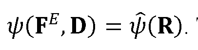 This is similar to the isotropic case where the additional material frame invariance allows a model to choose ut and vt such that and

define

[0069] In some embodiments, another common stress measure may be the first Piola-
Kirchhoff stress, defined as and related to σ with . If F£D is


denoted with where

Here T and D are operators on matrices that keep upper triangular part and

diagonal part respectively.
[0070] 3.3.1 Codimensional Anisotropic Elasticity for Curves
[0071] Elastic curves may be modeled with rotational material symmetry around the fiber direction Dx. In other words, for curves, the material directions D2 and D3 may be regarded as essentially arbitrary, and any choices which are mutually orthogonal with Dx may give the same potential. Guided by this material symmetry,
 may be decomposed into a composition of three deformations, where the first (Rx) is a stretching of the fibers, the second (R2) is a shearing of the fibers and the third (R3) is a deformation of the cross section of the fibers:

Based on the decomposition, the elastic potential for curves may be expressed as a sum of 3 terms
 The first term penalizes

change of fiber length. The second term penalizes shearing along the
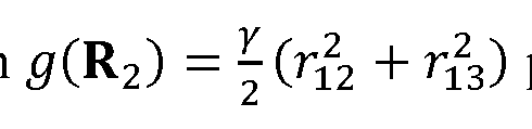
fibers. In absence of other deformations, a cross section of the fibers may behave like material in frictional contact, resisting compression and shearing. Thus, the third term /i(R3) may be a form of a two dimensional elastic potential, since it naturally enforces the frictional contact (when combined with appropriate plasticity law). That is,

where e1 and e2 are the logarithms of the nontrivial singular values of R3.

[0073] For the elastic surface energy, the surface may be assumed as being isotropic, e.g., the potential is invariant under rotation of the material directions D-,^ and D2 . Similarly, R = R3R2RX is decomposed into a composition of three deformations. The first (Rx) is an in- plane deformation of the surface. The second (R2) is a shearing of surface normal. The third
(R3) is a compression or stretching of the surface normal:

The energy may be expressed as a sum of three terms,
 The first term (R3) may penalize compression of the material in the normal direction, since the surface may be mostly surrounded by empty space which can expand freely:

[0074] The second term may be a form of to penalize shearing of the

normal to the surface. The third term hiR^ may use a two dimensional version of a fixed corotated potential to penalize deformation of the surface. Although in some embodiments, any in-plane energy may be used, with no change except to the stress and stress derivatives.
[0075] 3.4 Friction and Plastic Yield Condition
[0076] With Coulomb friction, the frictional force ff may be smaller than a constant cF (the coefficient of friction) times the normal force In a continuum view, at a given

point x in world space and a normal vector n, the traction vector t represents the local force per area that the material on one side of the plane with normal n exerts on the other side. The traction may have normal and shearing components

respectively where s(n, Θ) is an arbitrary vector in the plane with normal n, and Θ indicates its direction in the plane. Note that in the convention here, the compressive force fn may be positive as in the Coulomb model. If the material is in frictional contact in direction n, then ff = fs is the component of the frictional response in the direction s(n, Θ) and for angles Θ, and the inequality may be satisfied.

[0077] The traction may be expressed in terms of the Cauchy stress σ as t = ση, showing that the Coulomb model places constraints on the stress:
 for all Θ given frictional contact direction n. In the case of a grain, contact may be assumed to happen in all directions. For elastic surfaces or curves (e.g. clothing), the model considers the directions orthogonal to the manifold to be in frictional contact. Together with the choice of
elastic potential, this results in a less restrictive constraint that does not affect elastic deformation in the manifold. For frictional contact between surfaces, the model may consider contact in the direction normal to the surface: n = q3. For curves, there is a two dimensional normal space spanned by q2 and q3 and thus contact in all directions are considered
for all Θ given frictional contact direction n. In the case of a grain, contact may be assumed to happen in all directions. For elastic surfaces or curves (e.g. clothing), the model considers the directions orthogonal to the manifold to be in frictional contact. Together with the choice of
elastic potential, this results in a less restrictive constraint that does not affect elastic deformation in the manifold. For frictional contact between surfaces, the model may consider contact in the direction normal to the surface: n = q3. For curves, there is a two dimensional normal space spanned by q2 and q3 and thus contact in all directions are considered

[0078] In order to satisfy the stress constraints the material will yield. Physically this yielding may manifest as the cloth or fibers sliding, and "forgetting" some of the shearing deformation. This "forgetting" occurs by some of the incremental deformation being stored in Fp as opposed to F£, as the stress is a function of F£ and not Fp.
[0079] 4. DISCRETIZATION
[0080] In some embodiments, the disclosed approach may include MPM discretization, which translates from the theoretical continuum equations into a computation procedure for codimensional elasticity with contact. PIC and MPM may be hybrid particle/grid methods. From the continuum point of view, the particles represent discrete samples of the continuous material and the grid is a helper for computing their physical interactions. For example, for sands, the particles may be rendered as individual grains and the grid update, whose essential features are inherited from the continuum, which can be seen as a means for processing their frictional contact interactions. However, for codimensional elasticity, the continuum samples may be modeled as coherent surface or curve meshes, rather than as unstructured particles, which is different from other MPM approaches.
[0081] The disclosed MPM discretization may model self-collision and its ramifications in the grid momentum updates, as well as the associated elasticity and plasticity updates. In some embodiments, the discretization procedure may include:
[0082] (1) Transfer to grid: transferring mass and momentum from particles to the grid, and dividing grid momentum by grid mass to define grid velocity.
[0083] (2) Update grid momentum: using either explicit symplectic Euler or backward Euler to update grid momentum.
[0084] (3) Transfer to particles: using APIC to transfer velocities and affine matrices from grid to particles.
[0085] (4) Update particles: updating particles positions and deformation gradients.
[0086] (5) Update plasticity: projecting the deformation gradient for plasticity, and updating the elastic and plastic parts.
[0087] 4.1 Lagrangian State
[0088] In some embodiments, the Lagrangian particle state may be the primary representation of material for MPM. Particles can be classified as: (i) traditional MPM particles, (ii) Lagrangian mesh vertex particles, or (Hi) Lagrangian mesh element quadrature particles (e.g., see FIG. 11). Type (ii) particles may be used to track the in-manifold deformation of the elements. Type (Hi) particles may be used to track to the codimensional deformation in an updated Lagrangian manner.
[0089] At time tn, the model stores the particle positions velocities initial mass mp,


elastic deformation gradient initial volume affine velocity Cp and undeformed


material directions Dp. In some embodiments, Dp is not stored for particles of type (i) and (ii). is not stored for particles of type (ii). The mass is set as is set


according to the total volume divided by the number of particles for type (/') particles. For particles of type (ii) and (Hi), the volume of each triangle or segment is divided equally among the type (ii) and type (Hi) particles incident to it, and then is added to each particle's V°
[0090] Here the notation /( , Im, Im may be used to represent the sets of particle indices of types (i),(ii) and (Hi) respectively. E.g. for any particle index p, the particle is in one of /( ; /(") or depending on its type.
[0091] 4.2 Grid Transfers
[0092] 4.2.1 Particle to Grid
[0093] In some embodiments, the particle mass and momentum may be transferred to the grid using, e.g., APIC. Each particle p and grid node i is associated with a weight


b-spline kernels. These weights define the contribution of quantities on particle p to grid
node i. The mass contribution from particle p to grid node i is The total mass on grid

node i is a sum of the contributions from particles

[0094] With APIC, each particle also stores matrix to define an affine velocity local to the

particle. With this convention, the momentum contribution from particle p to node i is
For each grid node /', a sum of the contribution from particles

p is generated for grid momentum and then is divided by the grid mass to generate the grid velocity as

[0095] 4.2.2 Grid to Particle
[0096] After the update of grid node momentum, the grid velocities are transferred to particles. vf+1 denote grid node velocities after the momentum updates. The grid to particle transfer with APIC may be written as and
 where bd is the b-spline degree (bd = 3 for cubic

b-spline interpolation, bd = 2 for quadratic b-spline interpolation) and h is the Eulerian grid spacing. For the linear kernel reduces to the velocity gradient. In that case, it can be

computed as

[0097] For MPM particles and Lagrangian mesh vertex particles, the positions are updated with The positions of Lagrangian mesh element quadrature particles

are confined to (or around) the barycenters of their corresponding Lagrangian elements to prevent drifting that may occur with a MPM update of these positions.
[0098] 4.2.3 Dampening
[0099] In some embodiments, the Rigid Particle-in-Cell (RPIC) may be treated as a reduced APIC scheme that damps out stretching and shearing motions while conserving rigid velocity modes. APIC degrades to RPIC if just the skew symmetric part of is kept. Furthermore,

if is decomposed into the symmetric part and the skew symmetric part


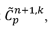 the model may stably introduce damping to the system by scaling


[00100] 4.3 Deformation Gradient Update
[00101] In some embodiments, the continuum samples may be treated as coherent surfaces or curves, rather than as unstructured particles. The treatment may be applied to, e.g., elastic volumes and surfaces (without self-collision). In some embodiments, for the meshes, the Eulerian MPM update of the deformation gradient may be abandoned, and the mesh connectivity may be used to compute the manifold components of the deformation gradient. This approach may also be applied to triangulated surfaces and segmented curves. This allows for a Lagrangian update of the deformation gradient that does not suffer from the numerical plasticity or fracture of the Eulerian update. The approach allows for coupling of Lagrangian elastic meshes with MPM materials. However, self-contact with codimensional meshes may not be well resolved.
[00102] In some embodiments, the disclosed approach further introduces an Eulerian deformation of the grid, to obtain the full rank deformation gradient. Thus, the disclosed approach allows for penalizing self-contact, while still preventing numerical plasticity and fracture. A comparison of the approaches with or without Eulerian deformation of the grid is shown in FIG. 10.
[00103] In some embodiments, the deformation gradient may be updated in terms of the motion of the grid over a time step. The motion of the grid may be described in terms of Xi , the Eulerian grid nodes at the beginning of the time step and xt their location after a grid update. Although the grid may not be necessarily deformed, the grid momentum update may be treated in terms of the motion that it may cause on the grid. In particular, this allows defining the elastic grid forces through a differentiation of a potential. The use of incremental grid node motion is referred to as an updated Lagrangian view. In other words, the motion of the grid is treated as Lagrangian, albeit from the grid configuration at time tn, instead of the rest configuration. Using to denote the grid node velocity after the momentum update,
 the locations are updated
 to denote the vector of all moved grid positions X; and velocities
 respectively, the deformation gradient update on particle p may be defined in terms of

[00104] For MPM particles (e.g., type (/')), the elastic deformation gradient may be updated as:
 where assuming no initial deformation. For mesh vertex

particles (e.g., type (/'/)), the deformation gradient may not be stored, so elastic deformation gradient may not be updated. For a Lagrangian mesh element quadrature particle (e.g., type

are matrices whose columns are respectively the deformed elastic and initial material directions. For the ζ (e.g., 1 for curves and 2 for surfaces) directions tangent to the manifold,
 which corresponds to the undeformed mesh element edge vectors (where β = 1, ... , ζ). Then which are

the deformed edge vectors. The deformed mesh particle positions are interpolated from the deformed grid node positions In some embodiments, the ζ directions

 tangent to the manifold may not include superscript E since they may not experience plasticity. Also, the notation mesh(p, β) for β = 0 . . . ζ is used to denote the mesh vertex particle (type (/'/)) indices of the mesh element corresponding to Lagrangian mesh element quadrature particle p. In some embodiments, the remaining 3 — ζ directions may be of unit length and normal to the manifold, and may be evolved as in MPM via

[00105] In some embodiments,
 is updated ignoring any further plasticity. may
 be further processed for plasticity to obtain

[00106] 4.4 Grid Momentum Update
[00107] In some embodiments, the update of the grid node momentum (e.g., velocities since the grid node masses do not change in the update) may be described as:

The hat in distinguishes the update from the velocities that may be transferred to the

grid in a next time step denote the vector of all grid moved positions and

 velocities respectively. The grid momentum update may be expressed as:
 where f is the elastic force, g is the gravitational acceleration and for symplectic Euler

or for backward Euler. The notation x(q) indicates the dependence of the moved grid

nodes through

[00108] The elastic force f may be defined in terms of the elastic potential energy. Given elastic energy density ψ, the total potential may be computed as over material

domain Ω. When discretely approximated on particles, the total potential may be expressed as:

where is the undeformed volume of particle p. To compute grid node forces, Φ is differentiated as a function of is expressed as a function of The force on node i is


expressed as

[00109] may be a third order tensor, and may not depend on
 because is linear

 in In some embodiments, the tensor allows splitting the computation into three parts. The first part corresponds to MPM particles and the force is
 - y expressing F using a material space coordinate frame which is aligned with the element, the first ζ columns of F may be assumed to correspond to in-manifold deformation. In other words, the first ζ columns of
correspond to the stress response inside the manifold and these terms can be computed by first computing forces on Lagrangian mesh vertex particles (type (/'/')) and then transferring them to the grid. Denoting these vertex forces with
- y expressing F using a material space coordinate frame which is aligned with the element, the first ζ columns of F may be assumed to correspond to in-manifold deformation. In other words, the first ζ columns of
correspond to the stress response inside the manifold and these terms can be computed by first computing forces on Lagrangian mesh vertex particles (type (/'/')) and then transferring them to the grid. Denoting these vertex forces with
 their corresponding contribution to grid node forces may be computed as The last 3— ζ columns

of correspond to the normal space contribution. This part may be computed by summing over Lagrangian mesh element quadrature particles (type (Hi)). Differentiating the last ζ columns of with respect to may be handled similarly to MPM through


This contribution to the force may be expressed as

where denotes the column of ΈΕ . With


this view, the force is expressed as

[00110] In some embodiments, when using backward Euler, the system may be modeled by utilizing the Hessian of Φ with respect to
 and ignoring the effects of plasticity during the process. The action of this Hessian on an arbitrary increment Su may be expressed as where implicit summation

may be used on repeated indices. In some embodiments, Newton's method may be used to solve the nonlinear system. In some embodiments, the effects of plasticity may be included in the implicit solve. However, this leads to non-symmetric force derivatives that require a generalized minimal residual method (GMRES) when using Newton's method. According to at least some embodiments of the present disclosure, the lagged plasticity approach may lead to symmetric force derivatives and thus a minimal residual method (MINRES) may be used to solve the linearized systems.
[00111] 4.5 Return Mapping
[00112] In some embodiments, the return mapping may be a discrete version of the yield condition and flow rule. The return mapping may be a form of a projection, which enforces the yield condition on the stress, with the direction of the flow rule, defining the direction of the projection. The return mapping may be applied after the deformation gradient update so that the updated stress may satisfy the yield condition. To perform the return mapping, the QR-decomposition may be generated as
 is projected from to satisfy the yield condition, before constructing In some
 embodiments, the stress satisfies for every normal n to the curve,

and every tangential direction s(n, Θ) perpendicular to
 denotes the stress evaluated at
 (the hypothetical stress if no plastic flow occurs), while σ denotes the stress evaluated at Rn+1 (the stress accounting for plasticity); similar naming conventions apply to the and
 fn, and other hatted and non-hatted variables.
[00113] 4.5.1 Surfaces
[00114] In some embodiments, for surfaces, the normal may be fixed n = q3, and s(n, Θ) may be eliminated by noting that maximum of s(n, θ)τ t is obtained at the angle corresponding to the projection of t into the plane with normal n: maxg s(n, 6)Tt = It + y^nl . The model determines if r33 > 1, if the normal is in extension and no friction should occur, r13 = r23 = 0 is set. Further, r33 = 1 may be set, as it is used to penalize collisions and previous stretching in that direction may not be taken into account. If f33 < 1, the model determines whether the condition |t— (tTn)n| + cFnTt < Ois satisfied, where n = q3. The traction may be expressed as

Thus the magnitude of the normal traction may be expressed as

and the magnitude of the tangential traction may be expressed as If

the condition is violated, uniform scaling may be applied: and


so that The r13and r23 components are changed, as these represent

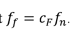
shearing along the surface of, e.g., clothing. In some embodiments, the magnitude of the tangential traction may change, but the direction may not change, corresponding to the uniform scaling. In some embodiments, the return mapping may be independent of the choice of in-plane energy /i(Ri). E.g., the in-plane surface energy may be used from instead.
[00115] FIG. 16 illustrates the return mapping of a 2D curve. is unchanged. In the

left figure, each shaded region corresponds to the feasible state of the deformed material normal and is determined by the yield function. The right figure shows the same yield surface in r12r22 space. The tip of the yield surface corresponds to the world space manifold normal and is usually different from d2. For example, the Return mapping may take a trial strain and results in the The particle corresponding to is inside the yield

 surface and exhibits an elastic response. The particle corresponding to
 is under compression but experiences more shear than friction allows. Such a configuration is projected to the yield surface along the direction that avoids normal component change. The particle corresponding to
 is experiencing tension and is projected to the tip of the yield surface. The corresponding stress is zero, allowing materials to separate freely. The particle corresponding to
 is inverted from the original side of material (due to discrete numerical step). The shearing may be disabled by nullifying the r22 component, and relying on elasticity to penalize such configuration.
[00116] 4.5.2 Curves
[00117] Fibrous materials may have anisotropic friction. For example, hair may be smoother along the fiber direction than perpendicular to the fiber direction. Thus, an anisotropic friction rule may be used, which is stricter and easier to apply. Let

be the entries of σ in the Q basis, and
 Then the conditions are which is Mohr-Coulomb in the q2, q3 plane, and


which controls the friction along the fiber, and β are material

parameters. Larger increases friction perpendicular to the fibers, and larger β increases friction along the fiber.
[00118] The stricter conditions imply that

β. The direction s(n, Θ) may be written as

q3 plane. Thus,

from the derivation of 2D Mohr-Coulomb. Therefore


which may be less or equal to 0 by assumption.

[00119] To enforce these constraints, the 2D volume preserving return mapping may be performed on
 The mapping may be described in terms of the logarithms of

the singular values of
 The model determines if

0, in which case the hair has expanded laterally and no friction should occur and

0. Otherwise the model determines
 f which corresponding to a situation where no plasticity occurs and Otherwise plastic flow occurs
 and are set, which will preserve In some


embodiments, the model may choose to make


condition is violated, scaling is performed
 to satisfy


[00120] 5. SIMULATION SAMPLES
[00121] Table 1 lists parameter choices for some simulation examples. Table 2 lists runtime performance results for some simulation examples. In some embodiments, some simulations may be run on Intel Xeon E5-2690 V2 with 19 threads.

Table 1. Parameter choices. Material Parameters: Here p refers to the density, E to the Young's modulus, η to the Poisson's ratio, y to the shearing stiffness, k to the stiffness, <t>F to the internal friction angle, and v to the damping coefficient. For surfaces, the friction coefficient CF = tan <t>F. For curves, the friction coefficient along the fiber is β = tan <t>F.
The one perpendicular to the fiber is

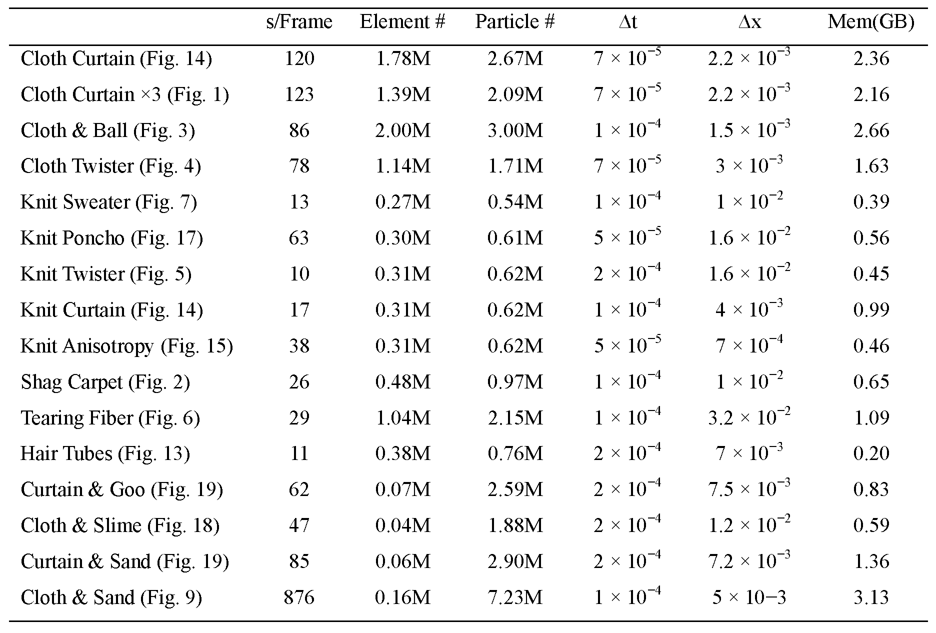
Table 2. Runtime performance results for some simulation examples. Element # denotes number of triangles (for surfaces), number of segments (for curves) or the total count (for coupling simulations). Memory usage is measured in the end of the first frame. At here means maximum allowed time step. The actual running At is adaptive and may be restricted by Courant-Friedrichs-Lewy (CFL) condition when the particle velocities are high. In the simulations, a CFL number equals to 0.3, e.g., particles are not allowed to move further than 0.3Δχ in a time step.
[00122] 5.1 Effect of Friction
[00123] FIG. 12 illustrates a simulation of 2D curves with different friction coefficients dropping on a block. Internal friction may be naturally controlled via adjusting cF.
[00124] 5.2 Simulation of Cloth
[00125] The surface elastoplasticity model may simulate cloth triangulated surfaces in
various scenarios involving numerous self-collisions (see, e.g., FIG. 1, FIG. 3, FIG. 4 and FIG. 14). The elastoplasticity model can resolve frictional contacts with a modest computational cost. The run time may not grow with the number of colliding primitives. In some embodiments, for the cloth examples, zero friction (cF = 0 and γ = 0) may be chosen to allow smooth sliding between cloth pieces.
[00126] 5.3 Simulation of Knitted Garments, Hair and Fibers
[00127] The fiber elastoplasticity may be simulated with yarn level simulation of knitted fabric. In some embodiments, multiple threads per yarn may be simulated. A mesh model may be used to simulate different examples including, e.g., dropping a sweater (FIG. 7), a jumping character wearing a poncho (FIG. 17), twisting a knitted cloth with a cylinder (FIG. 5), and hitting a knitted cloth curtain with a ball (FIG. 14). By accurately capturing frictional contact between yarns, the method inherently reproduces anisotropic stretching behaviors governed by knit patterns (FIG. 15). The fiber model may also be suitable for simulating hair (FIG. 13), shag carpet (FIG. 2) and other fibrous materials (FIG. 6). In some embodiments, each strand may be simulated. At least in some embodiments, the disclosed method scales well regardless of the complexity of segment contacts. RPIC damping may be used for stabilizing the simulations under large timesteps.
[00128] 5.4 Two-way Coupling
[00129] The disclosed method inherently handles multiple material coupling without requiring additional treatment. The constitutive model may be defined on each particle. For example, FIG. 1 and FIG. 9 illustrates a sand column with 7 millions particles coupled with a piece of cloth. FIG. 19 illustrates a cloth curtain getting hit by a ball while interacting with sand and/or goo. FIG. 18 illustrates dripping viscous green slime into an elastic bear geometry. A relatively high collision stiffness (k) may be set on the cloth to prevent sand from sticking to it.
[00130] 5.5 Comparison with other MPM Methods
[00131] The result of disclosed method is compared with other MPM approaches by simulating multiple curves dropping onto a block (see FIG. 10). Other meshless MPM causes numerical fracture of the material. The other method may just model the manifold stress response, resulting in unnatural clumping and numerical cohesion of curves. The disclosed
method adopts a full elastoplasticity model, achieves natural and realistic dynamics, and exhibits a smooth frictional sliding appearance, without excessive frictional effects.
[00132] 6. ADDITIONAL TREATMENT
[00133] In some embodiments, the disclosed method may use a regular grid to resolve material interactions. The apparent thickness of the surface and/or curve may depend on the grid resolution and on the repulsion energy model. In some embodiments, the disclosed method may be modified to reduce or eliminate artifacts when if the grid resolution is large. For a large grid resolution, the artifacts may manifest as numerical separation where particles tend to stay separated by an amount about half a grid cell width or numerical stickiness. Thus, the motion of the grid may be accurate to resolve the proper behavior. Therefore the method may simulate frictionless materials and control the apparent thickness independent of the grid.
[00134] In some embodiments, the disclosed method is suitable for situation where the size of the surface or curve elements is at most the size of the grid spacing. In some embodiments, the disclosed method may be modified to reduce or eliminate persistent wrinkles, which may manifest when a mesh is fine compared to the grid. In some embodiments, the disclosed method may be modified to reduce or eliminate self-penetration, which may manifest when a mesh is coarse compared to the grid because the material coverage is not resolved well enough on the grid. When penetration accidentally happens (due to At being too big), it may be resolved because elasticity may penalize that inverted collision direction. In some embodiments, the disclosed method may prevent the self- penetration by enforcing the CFL condition when choosing At. The disclosed method may use small time steps and increase overall run time.
[00135] In some embodiments, when transferring from particles to grid, the disclosed method may determine local neighbor information. In some embodiments, the penalty on compression in the normal direction may be treated as repulsion springs. In some embodiments, no fail-safe is used to prevent self-penetration when the repulsions fail. In some embodiments, the disclosed method may have smaller time steps for high grid resolution simulation, without fail-safes. In some embodiments, the disclosed method performs well for high resolution examples. E.g., for the cloth curtain example (FIG. 14), the disclosed method may achieve computation times of, e.g., 2 minutes per frame on average
for, e.g., 1.8 million triangles.
[00136] In some embodiments, the disclosed method tends to scale as well as the particle-grid transfers. The process may be performed in parallel over multiple CPU threads. In some embodiments, performance gains may be achieved with a GPU implementation.
[00137] In some embodiments, derived from a continuum, during the discretization of surface elasticity, material local to the surface moves in straight lines with the normal. In some embodiments, the continuum based bending model may be used.
[00138] 7. DETAILS OF MODELING PROCESSES
[00139] 7.1 OR Differentiation
[00140] In some embodiments,
 can be computed from F and
 This may be used for computing the linearized force in implicit time integration. If F = QR where Q is orthonormal with QTQ = I, and


where <5R is upper triangular:


[00141] These equations can be used to solve for Then constructing


[00142] The corresponding 2D result is

[00143] 7.2 Computing Stress

[00144] In some embodiments, the above holds for any
 that satisfy
 may be upper triangular. Specifically, it may be shown that given arbitrary upper triangular, 3δΈ such that


[00145] Using null for all upper triangular


If choosing in Equation (1), then
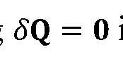

[00146] Since
 is any upper triangular matrix, have the same upper

triangular part. Furthermore, since RT is lower triangular, have the same

upper triangular part.
[00147] If the method chooses
 in Equation

then

[00148] Since is an arbitrary skew symmetric matrix (due to


[00149] In summary, have the same upper triangular part.

is symmetric. The tensor is denoted with


Therefore, A may be τ written in the Q basis.
[00150] 7.3 A Curve in 3D
[00151] The upper triangular part of A may be contstructed with , then

symmetry of A is used. Assuming
 then
then
 where
where

Then

[00152] Here, the process may choose
 to be the dilational part of the Kirchoff stress from the 2 x 2 Stvk Hencky Drucker-Prager. In other words, assuming getting some t after the return mapping of dry sand from an input
 the bottom right corner of A is replaced with pi, where p = tr(t) /2.
[00153] Under such a choice,

[00154] In some embodiments, Mohr friction criteria may lead to the following maximization: maximization of over all possible n that is perpendicular to

the fiber direction, with all d perpendicular to n and has unit length. In other words, is maximized over all possible n that is perpendicular to the fiber

direction, with all d perpendicular to n and has unit length.
[00155] Therefore,
 is maximized over all possible n that is perpendicular to the fiber direction, with all d perpendicular to n and has unit length, where
 Since in the discretization, the fiber direction is q1; therefore for some Θ.

[00156] Therefore,
 is maximized over possible n that is (0, c, s) over all 6>, with all
 perpendicular to n and has unit length.
[00157] Lagrangian multiplier may solve the maximization and lead to the maximum
If choosing g(x) = x, the yield surface may be The return


mapping is then simply a scaling on r so that the yield criteria is satisfied.
[00158] 7.4 A Surface in 3D
[00159] Surface may be similar to curve in the framework. With the codimensional discretization, the triangle may be mapped back to x-y plane. If the input 3D triangle at rest is
 the method may define This forms an imaginary
 whose QR decomposition leads to the rotation from x-y plane of this triangle
 as well as the top part of being the 2 X 2 version Dm. The third column of is the rotated D3 where
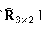

D3 = e3
[00160] In some embodiments, for any triangle di, d2 in world space, the full F may be constructed as:

[00161] In MPM, is upper triangular,

therefore is upper triangular.
[00162] The method performs thin QR decomposition:
 where may be 2 x 2 upper.
[00163] If = qx X q2 is constructed, then
 where Qh := d3. The QR decomposition of F is constructed as

Here

[00164] The previous lemma in curve may still hold: have the

same upper triangular part. is symmetric. This tensor may be denoted with A

· Therefore A may be τ written in the Q basis. The upper

triangular part of A may be constructed with then symmetry of A is used.


[00167] Physically, the top left is in plane (x-y) deformation of the triangle, since

r3 represents the deformation of D3 . because is the length change,

is the shearing (or the deviation from being perpendicular to the x-y triangle plane).

Shearing may also penalize length change.
[00168] Defining

then
 where
where

I (1(11691 Then,

[00170] In some embodiments, Mohr friction criteria leads to the following maximization: Maximization of
 over all possible n that is perpendicular to the manifold plane, with all d perpendicular to n and has unit length. In other words, is maximized over all possible n that is perpendicular to the

manifold plane, with all d perpendicular to n and has unit length. In other words,
is maximized over all possible n that is perpendicular to the manifold plane, with all

d perpendicular to n and has unit length, where

[00171] n perpendicular to manifold plane means for some k (unit

length constraint is extra).
 where is upper triangular 2 x 2 , this means for some z.

Therefore, Therefore


[00172] The process maximizes

for some Θ. The maximum is for

x < 1, 0 otherwise, g(x) = yx. When r33 > 1, / = 0, the maximum is yr33 |r| .
[00173] In this case, the return mapping causes r to be zero.
[00174] When r33 < 1, the maximum is

[00175] The yield surface is therefore

[00176] If r33 is negative (corresponding to inverted collision), the max may choose The return mapping is setting r to be 0. Otherwise, r may be scaled to satisfy


[00177] 7.5 A Curve in 2D
[00178] 2D derivation may follow 3D curve derivation: have the

same upper triangular part. is symmetric. This tensor may be denoted with

Therefore, A may be τ written in the Q basis.

[00179] The energy choice may be

then

[00180] In some embodiments, Mohr friction criteria may lead to the following maximization: maximization of over all possible n that is perpendicular to
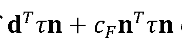
the fiber direction, with all d perpendicular to n and has unit length. In other words, is maximized over all possible n that is perpendicular to the fiber

direction, with all d perpendicular to n and has unit length. Therefore, is

maximized over all possible n that is perpendicular to the fiber direction, with all d perpendicular to n and has unit length, where
 Since in discretization, the fiber direction is qx, therefore

[00181] Thus,
 is maximized over
 In other words,
 is maximized over
 The maximum is otherwise.

[00182] When r22 > 1, h = 0, the maximum may be
 the return mapping may set r12 = 0. When r22 < 1, the maximum is
 The yield surface is therefore

[00183] If r22 < 0, the maximum may be The return mapping may set r12 = 0.

Otherwise, scale r12 may be scaled to satisfy


[00184] 7.6 Derivative of
 [00185] is a third order tensor, and does not depend on
 because is linear in


 Here the process performs the derivation, by definition

[00186] Plugging in:

[00187] Differentiating:

which may not depend on
 The undeformed segment or triangle may be treated as being aligned with the x-axis or xy-plane respectively. Thus, the initial F may no longer be I, but rather the rotation which maps the axis aligned element to its initial position in space. This is may not be an issue as the elastic energy density ψ may be world space rotation invariant. However, this allows assuming that D„ is block diagonal of the form
 for segments and

for triangles. This may save memory for Dp, and simplify computing
 [0018 Force on Grid

Define

Then


[00190] FIG. 20 is a high-level block diagram illustrating an example of a hardware architecture of a computing device 1100 that may perform various processes as disclosed, according various embodiments of the present disclosure. The computing device 1100 may execute some or all of the processor executable process operations or procedures described herein. In various embodiments, the computing device 1100 includes a processor subsystem that includes one or more processors 1102. Processor 1102 may be or may include, one or more programmable general-purpose or special-purpose microprocessors, digital signal processors (DSPs), programmable controllers, application specific integrated circuits (ASICs), programmable logic devices (PLDs), or the like, or a combination of such hardware based devices.
[00191] The computing device 1100 can further include a memory 1104, a network adapter 1110, a cluster access adapter 1112 and a storage adapter 1114, all interconnected by an interconnect 1108. Interconnect 1108 may include, for example, a system bus, a Peripheral Component Interconnect (PCI) bus, a HyperTransport or industry standard architecture (ISA)
bus, a small computer system interface (SCSI) bus, a universal serial bus (USB), or an Institute of Electrical and Electronics Engineers (IEEE) standard 1394 bus (sometimes referred to as "Firewire") or any other data communication system.
[00192] The cluster access adapter 1112 includes one or more ports adapted to couple the computing device 1100 to other devices. In the illustrated embodiment, Ethernet can be used as the clustering protocol and interconnect media, although other types of protocols and interconnects may be utilized within the cluster architecture described herein.
[00193] The computing device 1100 can be embodied as a single- or multi-processor storage system executing a storage operating system 1106 that can implement a high-level module, e.g., a storage manager, to logically organize the information as a hierarchical structure of named directories and files at the storage devices. The computing device 1100 can further include graphical processing unit(s) for graphical processing tasks or processing non-graphical tasks in parallel.
[00194] The memory 1104 can comprise storage locations that are addressable by the processor(s) 1102 and adapters 1110, 1112, and 1114 for storing processor executable code and data structures. The processor 1102 and adapters 1110, 1112, and 1114 may, in turn, comprise processing elements and/or logic circuitry configured to execute the software code and manipulate the data structures. The operating system 1106, portions of which is typically resident in memory and executed by the processors(s) 1102, functionally organizes the computing device 1100 by (among other things) configuring the processor(s) 1102 to invoke. It will be apparent to those skilled in the art that other processing and memory implementations, including various computer readable storage media, may be used for storing and executing program instructions pertaining to the disclosed technology.
[00195] The network adapter 1110 can include multiple ports to couple the computing device 1100 to one or more clients over point-to-point links, wide area networks, virtual private networks implemented over a public network (e.g., the Internet) or a shared local area network. The network adapter 1110 thus can include the mechanical, electrical and signaling circuitry included to connect the computing device 1100 to the network. Illustratively, the network can be embodied as an Ethernet network or a Fibre Channel (FC) network. A client can communicate with the computing device over the network by exchanging discrete frames or packets of data according to pre-defined protocols, e.g., TCP/IP.
[00196] The storage adapter 1114 can cooperate with the storage operating system 1106 to access information requested by a client. The information may be stored on any type of attached array of writable storage media, e.g., magnetic disk or tape, optical disk (e.g., CD- ROM or DVD), flash memory, solid-state disk (SSD), electronic random access memory (RAM), micro-electro mechanical and/or any other similar media adapted to store information, including data and parity information. The storage adapter 1114 can include multiple ports having input/output (I/O) interface circuitry that couples to the disks over an I/O interconnect arrangement, e.g., a conventional high-performance, Fibre Channel (FC) link topology. In various embodiments, the cluster adapter 1112 and the storage adapter 1114 can be implemented as one adaptor configured to connect to a switching fabric, e.g., a storage network switch, in order to communicate with other devices and the mass storage devices.
[00197] Amounts, ratios, and other numerical values are sometimes presented herein in a range format. It is to be understood that such range format is used for convenience and brevity and should be understood flexibly to include numerical values explicitly specified as limits of a range, but also to include all individual numerical values or sub-ranges encompassed within that range as if each numerical value and sub-range is explicitly specified.
[00198] While the present disclosure has been described and illustrated with reference to specific embodiments thereof, these descriptions and illustrations do not limit the present disclosure. It should be understood by those skilled in the art that various changes may be made and equivalents may be substituted without departing from the true spirit and scope of the present disclosure as defined by the appended claims. The illustrations may not be necessarily drawn to scale. There may be distinctions between the artistic renditions in the present disclosure and the actual apparatus due to manufacturing processes and tolerances. There may be other embodiments of the present disclosure which are not specifically illustrated. The specification and drawings are to be regarded as illustrative rather than restrictive. Modifications may be made to adapt a particular situation, material, composition of matter, method, or process to the objective, spirit and scope of the present disclosure. All such modifications are intended to be within the scope of the claims appended hereto. While the methods disclosed herein have been described with reference to particular operations performed in a particular order, it will be understood that these operations may be combined, sub-divided, or re-ordered to form an equivalent method without departing from the teachings
of the present disclosure. Accordingly, unless specifically indicated herein, the order and grouping of the operations are not limitations of the present disclosure.
Claims
1. A method of visualizing a codimensional object having a frictional contact, comprising: transferring masses and momentums of a plurality of particles of the codimensional object to a grid including a plurality of grid nodes;
updating momentums of the grid nodes based on the transferred masses and momentums of the particles;
transferring the updated momentums of the grid nodes to the particles of the codimensional object;
updating positions of the particles and deformation gradients of the particles based on the updated momentums of the grid nodes;
projecting the deformation gradients for plasticity of the codimensional object;
updating elastic components and plastic components of the codimensional object; detecting a collision response of the codimensional object and tracking deformation of the codimensional object;
updating orthogonal components of the deformation gradients that correspond to an elastic response of the frictional contact of the codimensional object; and
outputting a visualization of the object based on the positions of the particles of the codimensional object.
2. The method of claim 1, wherein the collision response of the codimensional object is based on an elastoplastic constitutive model.
3. The method of claim 2, wherein the codimensional object is a codimensional elastic object, and deformation of the codimensional elastic object is tracked in a Lagrangian view.
4. The method of claim 2, wherein the elastoplastic constitutive model includes an anisotropic hyperelastic constitutive model that separately characterizes the collision response to at least one manifold strain, at least one shearing, and at least one compression.
5. The method of claim 4, wherein the at least one shearing and the at least one compression are in directions orthogonal to a manifold of the codimensional object for the at least one manifold strain.
6. The method of claim 4, wherein the anisotropic hyperelastic constitutive model includes a plastic flow that enforces a Coulomb friction inequality between shear and normal stresses in directions orthogonal to a surface or a curve of the codimensional object.
7. The method of claim 2, wherein the collision response is caused by a self-collision between portions of the codimensional object or a collision between the codimensional object and another codimensional object.
8. The method of claim 1, wherein the deformation gradients represent spatial derivatives of material deformation mapping of the codimensional object.
9. The method of claim 1, further comprising:
damping stretching motions or shearing motions of the codimensional object.
10. The method of claim 1, wherein the grid is represented as a Lagrangian mesh.
11. The method of claim 1, wherein the plastic components of the codimensional object are updated using a return mapping process.
12. The method of claim 1, further comprising:
determining a next time step;
repeating at the next time step the transferring masses and momentums of the particles of the codimensional object, the updating momentums of the grid nodes, the transferring the updated momentums of the grid nodes, the updating positions of the particles and the deformation gradients of the particles, the projecting the deformation gradients, and the updating elastic components and the plastic components of the codimensional object.
13. A non-transitory computer readable storage medium storing a program to render an animated elastoplastic object, the program comprising instructions executable by a processor to:
represent the animated elastoplastic object using a mesh representation including a plurality of particles, each particle of the particles including a mass and a momentum;
transfer the masses and momentums of the particles to a grid representation of the animated elastoplastic object, the grid representation including a plurality of grid nodes; update momentums of the grid nodes of the grid representation based on an elastic force;
transfer the momentums of the grid nodes to the particles of the mesh representation; tracking deformation of the animated elastoplastic object caused by a collision;
updating orthogonal components of deformation gradients that correspond to an elastic response of a frictional contact of the animated elastoplastic object;
determine updated positions of the particles of the mesh representation based on the transferred momentums; and
update a visualization of the animated elastoplastic object based on the updated positions of the particles.
14. The computer readable storage medium of claim 13, wherein the elastic force depends on an elastic deformation gradient.
15. The computer readable storage medium of claim 14, the instructions further comprising instructions to:
update the elastic deformation gradient based on motions of the grid nodes of the grid representation over a time step.
16. The computer readable storage medium of claim 15, the instructions further comprising instructions to:
project the elastic deformation gradient for modeling an elastic or plastic motion of the animated elastoplastic object.
17. The computer readable storage medium of claim 14, wherein the elastic deformation gradient is specified by a differentiation of an elastic potential energy.
18. The computer readable storage medium of claim 13, the instructions further comprising instructions to:
further update the momentums of the grid nodes of the grid representation based on a gravitational force.
19. The computer readable storage medium of claim 13, wherein each mass of a grid node of the grid nodes of the grid representation is contributed by masses of multiple particles of the particles of the mesh representation.
20. The computer readable storage medium of claim 13, wherein the momentums of the grid nodes of the grid representation are updated using a symplectic Euler approach or a backward Euler approach.
Priority Applications (1)
| Application Number | Priority Date | Filing Date | Title |
|---|---|---|---|
| US16/610,315 US11145099B2 (en) | 2017-05-17 | 2018-05-17 | Computerized rendering of objects having anisotropic elastoplasticity for codimensional frictional contact |
Applications Claiming Priority (2)
| Application Number | Priority Date | Filing Date | Title |
|---|---|---|---|
| US201762507740P | 2017-05-17 | 2017-05-17 | |
| US62/507,740 | 2017-05-17 |
Publications (1)
| Publication Number | Publication Date |
|---|---|
| WO2018213607A1 true WO2018213607A1 (en) | 2018-11-22 |
Family
ID=64274637
Family Applications (1)
| Application Number | Title | Priority Date | Filing Date |
|---|---|---|---|
| PCT/US2018/033226 Ceased WO2018213607A1 (en) | 2017-05-17 | 2018-05-17 | Computerized rendering of objects having anisotropic elastoplasticity for codimensional frictional contact |
Country Status (2)
| Country | Link |
|---|---|
| US (1) | US11145099B2 (en) |
| WO (1) | WO2018213607A1 (en) |
Cited By (3)
| Publication number | Priority date | Publication date | Assignee | Title |
|---|---|---|---|---|
| CN111159954A (en) * | 2020-01-02 | 2020-05-15 | 株洲时代新材料科技股份有限公司 | Free-form surface mesh layout and finite element analysis method, system and medium for elastic element |
| CN113361184A (en) * | 2021-05-19 | 2021-09-07 | 武汉大学 | Particle system macroscopic stress fluctuation prediction method based on convolutional neural network |
| CN113516742A (en) * | 2021-05-14 | 2021-10-19 | 网易(杭州)网络有限公司 | Model special effect production method, device, storage medium and electronic device |
Families Citing this family (5)
| Publication number | Priority date | Publication date | Assignee | Title |
|---|---|---|---|---|
| US12216969B2 (en) * | 2020-09-04 | 2025-02-04 | Nvidia Corporation | Methods of contact for simulation |
| US20230169242A1 (en) * | 2021-11-29 | 2023-06-01 | Tencent America LLC | Systems and methods of simulating drag-induced multiscale phenomena |
| US11966999B2 (en) * | 2022-03-04 | 2024-04-23 | Tencent America LLC | Real-time simulation using material point method on graphics processing units |
| CN115203847B (en) * | 2022-07-15 | 2024-05-28 | 燕山大学 | A simulation method of anisotropic phase-field fracture algorithm based on MPM |
| CN116484245B (en) * | 2023-04-11 | 2025-12-23 | 四川九洲电器集团有限责任公司 | Data field joint decision graph clustering method based on grid division |
Citations (3)
| Publication number | Priority date | Publication date | Assignee | Title |
|---|---|---|---|---|
| US20100277475A1 (en) * | 2009-05-04 | 2010-11-04 | Disney Enterprises, Inc. | Computer graphic system and method for simulating hair |
| US20150187116A1 (en) * | 2013-12-31 | 2015-07-02 | Disney Enterprises, Inc. | Material point method for simulation of granular materials |
| US20150242546A1 (en) * | 2014-02-21 | 2015-08-27 | Inyong JEON | Method of Cloth Simulation using Constrainable Multigrid |
Family Cites Families (1)
| Publication number | Priority date | Publication date | Assignee | Title |
|---|---|---|---|---|
| US9245379B2 (en) * | 2011-10-19 | 2016-01-26 | Disney Enterprises, Inc. | Continuum based model for position based dynamics |
-
2018
- 2018-05-17 WO PCT/US2018/033226 patent/WO2018213607A1/en not_active Ceased
- 2018-05-17 US US16/610,315 patent/US11145099B2/en not_active Expired - Fee Related
Patent Citations (3)
| Publication number | Priority date | Publication date | Assignee | Title |
|---|---|---|---|---|
| US20100277475A1 (en) * | 2009-05-04 | 2010-11-04 | Disney Enterprises, Inc. | Computer graphic system and method for simulating hair |
| US20150187116A1 (en) * | 2013-12-31 | 2015-07-02 | Disney Enterprises, Inc. | Material point method for simulation of granular materials |
| US20150242546A1 (en) * | 2014-02-21 | 2015-08-27 | Inyong JEON | Method of Cloth Simulation using Constrainable Multigrid |
Non-Patent Citations (3)
| Title |
|---|
| GUILKEY ET AL.: "Implicit time integration for the material point method: Quantitative and algorithmic comparisons with the finite element method", INTERNATIONAL JOURNAL FOR NUMERICAL METHODS IN ENGINEERING, vol. 57, no. 9, July 2003 (2003-07-01), pages 1323 - 1338, XP055560930, [retrieved on 20180719] * |
| NGUYEN ET AL.: "Modeling the anisotropic finite-deformation viscoelastic behavior of soft fiber- reinforced composites", INTERNATIONAL JOURNAL OF SOLIDS AND STRUCTURES, vol. 44, no. 25-26, 2007, pages 8366 - 8389, XP022318109, Retrieved from the Internet <URL:https://www.sciencedirect.com/science/article/pii/S0020768307002582> [retrieved on 20180719] * |
| PFAFF ET AL.: "Lagrangian Vortex Sheets for Animating Fluids", ACM TRANSACTIONS ON GRAPHICS (TOG), vol. 31, no. 4, July 2012 (2012-07-01), XP055560902, Retrieved from the Internet <URL:https://dl.acm.org/citation.cfm?id=2185608> [retrieved on 20180719] * |
Cited By (4)
| Publication number | Priority date | Publication date | Assignee | Title |
|---|---|---|---|---|
| CN111159954A (en) * | 2020-01-02 | 2020-05-15 | 株洲时代新材料科技股份有限公司 | Free-form surface mesh layout and finite element analysis method, system and medium for elastic element |
| CN111159954B (en) * | 2020-01-02 | 2023-04-14 | 株洲时代新材料科技股份有限公司 | Free-form surface mesh layout and finite element analysis method, system and medium for elastic element |
| CN113516742A (en) * | 2021-05-14 | 2021-10-19 | 网易(杭州)网络有限公司 | Model special effect production method, device, storage medium and electronic device |
| CN113361184A (en) * | 2021-05-19 | 2021-09-07 | 武汉大学 | Particle system macroscopic stress fluctuation prediction method based on convolutional neural network |
Also Published As
| Publication number | Publication date |
|---|---|
| US11145099B2 (en) | 2021-10-12 |
| US20200082589A1 (en) | 2020-03-12 |
Similar Documents
| Publication | Publication Date | Title |
|---|---|---|
| Jiang et al. | Anisotropic elastoplasticity for cloth, knit and hair frictional contact | |
| US11145099B2 (en) | Computerized rendering of objects having anisotropic elastoplasticity for codimensional frictional contact | |
| Li et al. | An implicit frictional contact solver for adaptive cloth simulation | |
| Bender et al. | A survey on position‐based simulation methods in computer graphics | |
| Han et al. | A hybrid material point method for frictional contact with diverse materials | |
| Bender et al. | Position-based simulation of continuous materials | |
| Bender et al. | Position-based Methods for the Simulation of Solid Objects in Computer Graphics. | |
| Spillmann et al. | An adaptive contact model for the robust simulation of knots | |
| Zong et al. | Neural stress fields for reduced-order elastoplasticity and fracture | |
| Bargteil et al. | Animation of deformable bodies with quadratic Bézier finite elements | |
| WO2008013741A2 (en) | Physical simulations on a graphics processor | |
| Borycki et al. | GASP: Gaussian Splatting for physics-based simulations | |
| Jones et al. | Deformation embedding for point-based elastoplastic simulation | |
| He et al. | Projective peridynamics for modeling versatile elastoplastic materials | |
| Kikuuwe et al. | An edge-based computationally efficient formulation of Saint Venant-Kirchhoff tetrahedral finite elements | |
| JP2009529161A (en) | A method for simulating deformable objects using geometry-based models | |
| Cetinaslan | Position‐Based Simulation of Elastic Models on the GPU with Energy Aware Gauss‐Seidel Algorithm | |
| Gao et al. | Accelerating liquid simulation with an improved data‐driven method | |
| Garstenauer et al. | A unified framework for rigid body dynamics | |
| CN119784911B (en) | Particle collision method, device, equipment and storage medium based on physical simulation | |
| Cetinaslan | ESPEFs: Exponential spring potential energy functions for simulating deformable objects | |
| Oh et al. | Practical simulation of hierarchical brittle fracture | |
| Cao et al. | Research of fast cloth simulation based on mass-spring model | |
| Harmon | Robust, efficient, and accurate contact algorithms | |
| Fang et al. | Enhanced material point method with affine projection stabilizer for efficient hyperelastic simulations |
Legal Events
| Date | Code | Title | Description |
|---|---|---|---|
| 121 | Ep: the epo has been informed by wipo that ep was designated in this application |
Ref document number: 18801961 Country of ref document: EP Kind code of ref document: A1 |
|
| NENP | Non-entry into the national phase |
Ref country code: DE |
|
| 122 | Ep: pct application non-entry in european phase |
Ref document number: 18801961 Country of ref document: EP Kind code of ref document: A1 |