WO2017183076A1 - 在庫量算出装置、在庫量算出方法、及びプログラム - Google Patents
在庫量算出装置、在庫量算出方法、及びプログラム Download PDFInfo
- Publication number
- WO2017183076A1 WO2017183076A1 PCT/JP2016/062231 JP2016062231W WO2017183076A1 WO 2017183076 A1 WO2017183076 A1 WO 2017183076A1 JP 2016062231 W JP2016062231 W JP 2016062231W WO 2017183076 A1 WO2017183076 A1 WO 2017183076A1
- Authority
- WO
- WIPO (PCT)
- Prior art keywords
- inventory
- time
- processing
- processing time
- distribution
- Prior art date
- Legal status (The legal status is an assumption and is not a legal conclusion. Google has not performed a legal analysis and makes no representation as to the accuracy of the status listed.)
- Ceased
Links
Images




Classifications
-
- G—PHYSICS
- G05—CONTROLLING; REGULATING
- G05B—CONTROL OR REGULATING SYSTEMS IN GENERAL; FUNCTIONAL ELEMENTS OF SUCH SYSTEMS; MONITORING OR TESTING ARRANGEMENTS FOR SUCH SYSTEMS OR ELEMENTS
- G05B19/00—Program-control systems
- G05B19/02—Program-control systems electric
- G05B19/418—Total factory control, i.e. centrally controlling a plurality of machines, e.g. direct or distributed numerical control [DNC], flexible manufacturing systems [FMS], integrated manufacturing systems [IMS] or computer integrated manufacturing [CIM]
-
- Y—GENERAL TAGGING OF NEW TECHNOLOGICAL DEVELOPMENTS; GENERAL TAGGING OF CROSS-SECTIONAL TECHNOLOGIES SPANNING OVER SEVERAL SECTIONS OF THE IPC; TECHNICAL SUBJECTS COVERED BY FORMER USPC CROSS-REFERENCE ART COLLECTIONS [XRACs] AND DIGESTS
- Y02—TECHNOLOGIES OR APPLICATIONS FOR MITIGATION OR ADAPTATION AGAINST CLIMATE CHANGE
- Y02P—CLIMATE CHANGE MITIGATION TECHNOLOGIES IN THE PRODUCTION OR PROCESSING OF GOODS
- Y02P90/00—Enabling technologies with a potential contribution to greenhouse gas [GHG] emissions mitigation
- Y02P90/02—Total factory control, e.g. smart factories, flexible manufacturing systems [FMS] or integrated manufacturing systems [IMS]
Definitions
- the present invention relates to an inventory amount calculation device, an inventory amount calculation method, and a program.
- drum buffer rope (DBR (Drum Buffer Rope)) based on the TOC (Theory Of Constraints) as a method for managing productivity and in-process inventory.
- DBR Dynamic Buffer Rope
- TOC Theory Of Constraints
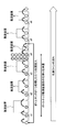
- FIG. 1 is a diagram for explaining DBR.
- FIG. 1 shows a production line that includes manufacturing apparatuses 1 to 6 and that processes materials in the order of manufacturing apparatuses 1 to 6.
- the manufacturing apparatuses 1 to 6 perform steps 1 to 6 in order.
- the inventory area a1 indicates the inventory area at the head of the production line, and the inventory areas a2 to a6 indicate inventory areas between the manufacturing apparatuses.
- the size of the rectangle indicating each manufacturing apparatus indicates the production capacity of each manufacturing apparatus. Therefore, the process 4 of the manufacturing apparatus 4 corresponding to the smallest rectangle is a bottleneck process.
- the bottleneck process is a process in which the processing time per material is the longest.
- DBR materials are input to the production line according to the production capacity of the bottleneck process. That is, one material is put into the production line at the timing when the bottleneck process ends one process. By doing so, the in-process inventory amount can be kept constant.
- the processing time of each manufacturing apparatus constituting the production line is not necessarily constant. This is because processing stoppage or delay due to so-called “choco stop” occurs.
- DBR explains the necessity of in-process inventory before the bottleneck process in order to prepare for the uncertainty of the processing time of each process.
- the shaded circles indicate the in-process inventory before the bottleneck process.
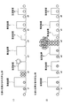
- FIG. 2 is a diagram for explaining the necessity of in-process inventory before the bottleneck process.
- (1) shows a problem when the in-process inventory is too small.
- the manufacturing apparatus 4 in the bottleneck process is idle due to a slight processing delay of the manufacturing apparatus (the manufacturing apparatus 2 in FIG. 2) related to any process before the bottleneck process.
- productivity decreases.
- the DBR only qualitatively refers to the appropriate amount of in-process inventory and does not quantitatively determine it. Therefore, conventionally, the amount of in-process inventory is determined based on experience and intuition.
- an object of one aspect is to quantitatively determine the in-process inventory.
- the inventory calculation apparatus may perform the process before the predetermined process from the first process of the production line based on a probability distribution of processing times of the plurality of processes performed before the predetermined process in the production line. Based on the first calculation unit that calculates the time required for the processing until each of the plurality of materials, the distribution of the required time calculated for the plurality of materials, and the processing time of the predetermined process, A second calculation unit that calculates an in-process inventory amount in the plurality of steps.
- the in-process inventory amount can be obtained quantitatively.
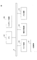
- FIG. 3 is a diagram illustrating a hardware configuration example of the inventory amount calculation apparatus according to the first embodiment.
- 3 includes a drive device 100, an auxiliary storage device 102, a memory device 103, a CPU 104, an interface device 105, and the like that are mutually connected by a bus B.
- a program for realizing processing in the inventory quantity calculation device 10 is provided by the recording medium 101.
- the recording medium 101 on which the program is recorded is set in the drive device 100, the program is installed from the recording medium 101 to the auxiliary storage device 102 via the drive device 100.
- the program need not be installed from the recording medium 101 and may be downloaded from another computer via a network.
- the auxiliary storage device 102 stores the installed program and also stores necessary files and data.
- the memory device 103 reads the program from the auxiliary storage device 102 and stores it when there is an instruction to start the program.
- the CPU 104 executes a function related to the inventory quantity calculation device 10 in accordance with a program stored in the memory device 103.
- the interface device 105 is used as an interface for connecting to a network.
- An example of the recording medium 101 is a portable recording medium such as a CD-ROM, a DVD disk, or a USB memory.
- a portable recording medium such as a CD-ROM, a DVD disk, or a USB memory.
- an HDD Hard Disk Disk Drive
- flash memory or the like can be given. Both the recording medium 101 and the auxiliary storage device 102 correspond to computer-readable recording media.
- FIG. 4 is a diagram illustrating a functional configuration example of the inventory amount calculation apparatus according to the first embodiment.
- the inventory quantity calculation device 10 performs a simulation of a production line based on a probability density function (probability distribution) of processing time of each manufacturing device (each process) constituting the production line. Subsequently, the inventory quantity calculation apparatus 10 estimates the distribution of the time required for the material to reach the bottleneck process from the production line input port. The inventory quantity calculation device 10 determines the in-process inventory quantity based on the estimated distribution and the processing time of the bottleneck process.
- In-process inventory refers to materials that are in the manufacturing process (between the first process and the last process) on the production line.
- the in-process inventory amount means the number of in-process inventory.
- the inventory quantity calculation device 10 includes a simulation unit 11, a distribution estimation unit 12, an inventory quantity calculation unit 13, an output unit 14, and the like. Each of these units is realized by processing executed by the CPU 104 by one or more programs installed in the inventory amount calculation apparatus 10.
- the inventory quantity calculation device 10 also uses a simulation model storage unit 15 and a processing time distribution storage unit 16. Each of these storage units can be realized using, for example, a storage device that can be connected to the auxiliary storage device 102 or the inventory amount calculation device 10 via a network.
- the simulation model storage unit 15 stores information necessary for simulating the production line, such as the number of processing devices constituting the production line and the number of processing devices corresponding to the bottleneck process. In the present embodiment, it is assumed that the production line to be simulated is as shown in FIG.
- a plurality of materials may be processed at the same time in one process (the number of materials that can be processed at the same time is not necessarily one). Moreover, there may be no inventory area between some processes.
- the processing time distribution storage unit 16 stores information indicating the probability density function of the processing time of each manufacturing apparatus (each process) constituting the production line.
- the simulation unit 11 executes a simulation of the production line indicated by the information stored in the simulation model storage unit 15 and requires a period from when the material is input to the production line until the processing of the process immediately before the bottleneck process is completed. Time (hereinafter referred to as “processing time LT B ”) is calculated. The simulation is executed multiple times. In the simulation, the processing time per material by the manufacturing apparatus in each process follows the probability density function stored in the processing time distribution storage unit 16.
- the distribution estimation unit 12 estimates a probability density function (probability distribution) of the processing time LT B based on a plurality of simulation results.
- the inventory amount calculation unit 13 determines an appropriate value of the in-process inventory amount before the bottleneck process (hereinafter, Calculated as “appropriate inventory”. Specifically, the appropriate inventory amount is calculated by dividing the upper ⁇ percentage point of the probability density function of the processing time LT B by the processing time t B.
- the appropriate inventory quantity is an inventory quantity that makes the in-process inventory quantity as small as possible. Strictly speaking, the appropriate inventory amount is the in-process inventory amount before the bottleneck process when the process of the bottleneck process is allowed to be delayed by the influence of the process before the bottleneck process with a probability of ⁇ out of 100 times. It is. Note that the processing time t B and the value of ⁇ are set in advance. For example, the processing time t B may be an average value of past processing times of the bottleneck process.
- the output unit 14 outputs the appropriate inventory amount calculated by the inventory amount calculation unit 13.
- ⁇ days per 100 days An example of obtaining an appropriate inventory amount when the stipulation is allowed will be described.
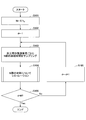
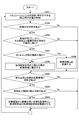
- FIG. 5 is a flowchart for explaining an example of a processing procedure executed by the simulation unit.
- step S ⁇ b > 101 the simulation unit 11 substitutes the calculation result of T / t B for the variable N.
- N is the number of processed materials for one day in the production line.
- T is the operating time of one day. That is, the processing number of one day materials, the operating time of the day, determined by dividing the processing time t B of the bottleneck process.
- the simulation unit 11 assigns 1 to the variable d (S102).
- the variable d is a variable for storing the number of simulation repetitions for one day. That is, the value of the variable d indicates how many days (how many times) the simulation is being executed when one day of simulation is performed once.
- the simulation unit 11 calculates N processing times for each manufacturing apparatus in the process before the bottleneck process based on the probability density function stored in the processing time distribution storage unit 16 for each manufacturing apparatus. Sampling is performed (S103). The N processing times are assigned an order from 1 to N.
- FIG. 6 is a diagram for explaining sampling of processing time.
- the upper graph shows the probability density function of the processing time of each manufacturing apparatus.
- probability density functions corresponding to the number of manufacturing apparatuses in the process before the bottleneck process are stored in the processing time distribution storage unit 16.
- the lower table shows the processing time sampled from the probability density function. N processing times are sampled from one probability density function.
- the simulation unit 11 executes a production line simulation to calculate the processing time LT B before the bottleneck process for N materials (S104).
- N is the number of processed materials for one day. Therefore, in step S104, one day of simulation is executed.
- N LT Bs are calculated.
- the calculated LT B is stored in the auxiliary storage device 102.
- FIG. 7 is a diagram illustrating a processing time before the bottleneck process.
- the processing time LT B of one material A is shown.
- the processing time LT B of the material A is an elapsed time from when the material A is input to the manufacturing apparatus 1 corresponding to the process 1 until the processing of the manufacturing apparatus 3 corresponding to the last process 3 before the bottleneck process is completed. It is.
- the simulation unit 11 determines whether or not the value of the variable d has reached M (S106).
- steps S103 and S104 are repeated M times (Yes in S106), the simulation ends. That is, the simulation for M days is executed. As a result, N ⁇ M processing times LT B are calculated.
- FIG. 8 is a flowchart for explaining an example of the processing procedure of the production line simulation.
- the following processing is executed for each manufacturing apparatus (each process) before the bottleneck process.
- step S201 the simulation unit 11 advances the simulation time (the time common to each process) by one unit.
- the simulation time is referred to as “simulation time”.
- the simulation unit 11 determines whether or not there is a material being processed in the target process (S202). When there is no material being processed (No in S202), the simulation unit 11 determines whether or not there is a material in an inventory area between the process immediately before the target process (S203).
- the simulation unit 11 determines whether or not the material can be carried into the target process (S204). That is, it is determined whether or not the number of materials currently being processed in the target process is less than the maximum value of materials that can be processed simultaneously in the target process. It should be noted that the number of materials currently being processed does not include the material that is the object of determination of whether or not it can be carried in.
- the maximum value is stored in advance in the simulation model storage unit 15 for each process.
- the simulation unit 11 If the material cannot be carried into the target process (No in S204), the simulation unit 11 returns to Step S201.
- the simulation unit 11 carries the material in order from the stock area with the process immediately before the target process, and is processing the material. (S205).
- the processing times in the order corresponding to the material among the processing times sampled in step S103 of FIG. 5 are associated with the material.
- the manufacturing apparatus 1 corresponds to the target process and the material is the nth (1 ⁇ n ⁇ N) th material
- the processing time sampled nth for the manufacturing apparatus 1 is associated with the material n.
- the current simulation time is associated with the material n as the processing start time of the material n in the target process.
- a plurality of materials may be loaded within the range of the maximum number that can be processed simultaneously by the target process.
- step S202 when there is a material being processed in the target process (Yes in S202), the simulation unit 11 has a material that has been processed in the target process among the materials being processed in the target process, and Then, it is determined whether or not the material whose order is earlier than the material is in the target process (S206). Whether a target process has been completed for a material is whether the elapsed time from the processing start time associated with the material in the target process has reached the processing time associated with the material in the target process It can be determined based on whether or not.
- step S203 If there is no corresponding material (No in S206), the process proceeds to step S203.
- the simulation unit 11 sets the corresponding material to the next process. It is carried out to the stock area (S208).
- the simulation unit 11 records the processing time LT B of the corresponding material in, for example, the auxiliary storage device 102 (S209).
- the processing time LT B of the material can be calculated by subtracting the processing start time associated with the material in the first step from the current simulation time.
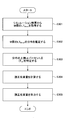
- FIG. 9 is a flowchart for explaining an example of a processing procedure executed by the inventory quantity calculation device based on the simulation result.
- step S301 the distribution estimation unit 12 sets the processing time LT Bmax that is the maximum value for every N pieces (that is, every day) out of the N ⁇ M processing times LT B recorded in the simulation. get. Therefore, M processing times LT Bmax are acquired.
- M processing times LT Bmax are acquired among the N ⁇ M processing times LT B .
- relatively large M values are extracted because, in the present embodiment, the distribution where the processing time LT B is large is of interest. This is because it is desired to obtain a detailed probability density function for a place where the processing time LT B is long.
- the reason why the processing time LT B is large is that the appropriate inventory amount is calculated based on the upper ⁇ percentage point in the probability density function of the processing time LT Bmax .
- the distribution estimating unit 12 based on the M processing time LT Bmax, to estimate the probability density function of the processing time LT Bmax (S302).
- the probability density function can be estimated using a known method. For example, a parameter of a normal distribution or other probability density function may be estimated based on M processing times LT Bmax .
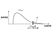
- FIG. 10 is a diagram illustrating an example of an estimation result of the probability density function of the processing time LT Bmax .
- the probability density function is a curve whose area is 1 with the horizontal axis as the processing time and the vertical axis as the probability density.
- the inventory quantity calculation unit 13 specifies the upper ⁇ percentage point of the probability density function (S303). That is, on the upper side of the probability density function of FIG. 10, the processing time T ⁇ at which the area is ⁇ percent is specified.
- the upper ⁇ percentage point of the probability density function may be calculated by the following procedures (1) to (3) instead of steps S302 and S303.
- the kth is y k and the k + 1 is y k + 1 .
- K is an integer part of M ⁇ ⁇ / 100.
- (3) The calculation result of (1 ⁇ e) ⁇ y k + e ⁇ y k + 1 is set as the upper ⁇ percentage point.
- e is a decimal part of M ⁇ ⁇ / 100.
- the inventory quantity calculation unit 13 calculates an appropriate inventory quantity based on the following equation (1) (S304).
- Proper inventory quantity T ⁇ / t B (1) That is, the appropriate inventory amount is calculated by dividing the upper ⁇ percentage point of the probability density function of LT Bmax by the processing time t B of the bottleneck process.
- Expression (1) is an expression for the purpose of calculating an inventory amount for preventing the bottleneck process from playing. For example, when the processing time before the bottleneck process is 1 hour and the processing time of the bottleneck process is 10 minutes, the material for one hour needs to exist before the bottleneck process. . If there is only 0.5 hours of material before the bottleneck process, the bottleneck process will be idle for 30 minutes while the process before the bottleneck process is processing for 1 hour. Therefore, according to the formula (1), it is possible to obtain an appropriate inventory amount that allows the probability of playing the bottleneck process to be ⁇ times in 100 times.
- ⁇ is considered to be 0.3% to 20%. This value is a value at which the probability of playing the bottleneck process is approximately once a year to once every five days.
- an appropriate in-process inventory that minimizes the in-process inventory while maintaining throughput (productivity).
- the quantity can be determined quantitatively.
- the functions of the inventory quantity calculation device 10 may be provided as a cloud service via a network such as the Internet.
- the distribution of the processing time LT B until the material put into the production line arrives just before the bottleneck process is obtained but there is an interest in obtaining the appropriate inventory amount, What needs to be determined with high accuracy is the distribution where the processing time LT B is large.
- the bottleneck process is the fourth process. That is, it is assumed that there are three processes (manufacturing apparatuses) before the bottleneck process.
- the probability density functions of the processing times stored in the processing time distribution storage unit 16 for the first to third manufacturing apparatuses (processes) are represented by p 1 (x), p 2 (x), and p 3 ( x).
- probability density functions adjusted to increase the probability that the processing time of the first to third manufacturing apparatuses (processes) is long are q 1 (x), q 2 (x), and q 3, respectively. (X). This is an artificially created probability density function for importance sampling. These probability density functions are also stored in the processing time distribution storage unit 16.
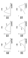
- FIG. 11 shows an example of p 1 (x), p 2 (x), and p 3 (x), and q 1 (x), q 2 (x), and q 3 (x).
- a processing time set X that is a vector of 3 ⁇ N elements is defined.
- X (x 1,1, x 1,2 , x 1,3, x 2,1, x 2,2, x 2,3, ⁇ , x N, 1, x N, 2, x N, 3 )
- x i, j indicates the processing time of the i-th material in the j-th manufacturing apparatus (process), and is sampled from the probability density function q j (x).
- the simulation unit 11 generates N ′ X, and samples N pieces of probability density functions q1 (x), q2 (x), and q3 (x) for each X. That is, in S103 of FIG. 5, the sampling sources are q 1 (x), q 2 (x), and q 3 (x). In step S106, it is determined whether d has reached N ′. Note that N ′ ⁇ M.
- step S301 in FIG. 9 L TBmax is acquired for every N pieces. Therefore, N ′ L TBmax is acquired.
- FIG. 12 is a diagram illustrating a method of calculating the upper ⁇ percentage point in the second embodiment.
- W k p (X k ) / (q (X k ) ⁇ N ′)
- An example of the calculation result of W k is shown in (1) of FIG.
- the simulation unit 11 sorts the sets of N ′ LT Bmax and W k in descending order of LT Bmax .
- An example of the sorting result is shown in (2) of FIG.
- FIG. 12 (2) shows an example of the calculation result of the cumulative weight Gl .
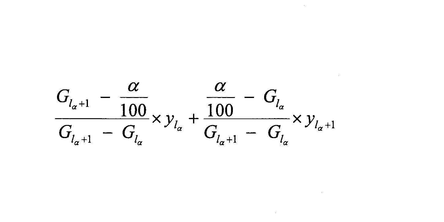
- the upper ⁇ percentage point of LT Bmax can be calculated by the following equation.
- G 1 ⁇ + 1 is the cumulative weight immediately after G 1 ⁇ .
- y 1 ⁇ + 1 is LT Bmax one after y 1 ⁇ .
- the simulation unit 11 is an example of a first calculation unit.
- the inventory quantity calculation unit 13 is an example of a second calculation unit.
- the bottleneck process is an example of a predetermined process.
- LT B is an example of the required time.
- LT Bmax is an example of the maximum value of the required time.
- the upper ⁇ percentage point is an example of “the upper probability is a predetermined value”.
Landscapes
- Engineering & Computer Science (AREA)
- General Engineering & Computer Science (AREA)
- Manufacturing & Machinery (AREA)
- Quality & Reliability (AREA)
- Physics & Mathematics (AREA)
- General Physics & Mathematics (AREA)
- Automation & Control Theory (AREA)
- General Factory Administration (AREA)
- Management, Administration, Business Operations System, And Electronic Commerce (AREA)
Abstract
在庫算出装置は、生産ラインにおける所定の工程の前に行われる複数の工程のそれぞれの処理時間の確率分布に基づいて、前記生産ラインの最初の工程から前記所定の工程の前までの処理の所要時間を、複数の材料のそれぞれについて算出する第1の算出部と、前記複数の材料に関して算出された前記所要時間の分布と、前記所定の工程の処理時間とに基づいて、前記複数の工程における仕掛かり在庫量を算出する第2の算出部と、を有する、ことで、仕掛り在庫量を定量的に求めることができる。
Description
本発明は、在庫量算出装置、在庫量算出方法、及びプログラムに関する。
生産性と仕掛り在庫量とを管理する手法として、TOC(Theory Of Constraints:制約条件の理論、制約理論)に基づいた、ドラム・バッファー・ロープ(DBR(Drum Buffer Rope))が有る。
図1は、DBRを説明するための図である。図1には、製造装置1~製造装置6を含み、製造装置1~6の順番で材料が処理される生産ラインが示されている。製造装置1~6は、順番に、工程1~6を実行する。また、在庫領域a1は、生産ラインの先頭の在庫領域を示し、在庫領域a2~a6は、各製造装置間の在庫領域を示す。また、各製造装置を示す矩形の大きさは、各製造装置の生産能力を示す。したがって、最小の矩形に該当する製造装置4の工程4が、ボトルネック工程となる。ボトルネック工程とは、材料1個あたりの処理時間が最長の工程をいう。
DBRでは、ボトルネック工程の生産能力に合わせて、生産ラインへ材料が投入される。すなわち、ボトルネック工程が1個の処理を終了したタイミングで1個の材料が生産ラインに投入される。そうすることで、仕掛り在庫量を一定に保つことができる。
ここで、生産ラインを構成する各製造装置のそれぞれの処理時間は、必ずしも一定ではない。いわゆる「チョコ停」による処理の停止や遅延等が発生するからである。
そこで、DBRでは、各工程の処理時間の不確実性に備えるため、ボトルネック工程前の仕掛り在庫の必要性を説いている。なお、図1において、網掛けが施された円は、ボトルネック工程前の仕掛かり在庫を示す。
図2は、ボトルネック工程前の仕掛かり在庫の必要性を説明するための図である。図2において、(1)は、仕掛かり在庫が少なすぎる場合の問題点を示す。この場合、ボトルネック工程の前のいずれかの工程に係る製造装置(図2では、製造装置2)のちょっとした処理の遅れにより、ボトルネック工程の製造装置4が遊んでしまう。その結果、生産性が低下するという問題が有る。
(2)は、仕掛かり在庫が多すぎる場合の問題点を示す。この場合、製造装置4が遊んでしまう可能性は低下するが、リードタイムが増大し、キャッシュフローの悪化や在庫管理が煩雑化するという問題が有る。
しかしながら、DBRでは、仕掛かり在庫の適正な量について、定性的に言及しているにとどまり、定量的には求めていない。そのため、従来は、経験や勘に基づき、仕掛かり在庫の量が決定されている。
そこで、一側面では、仕掛り在庫量を定量的に求めることを目的とする。
一つの案では、在庫算出装置は、生産ラインにおける所定の工程の前に行われる複数の工程のそれぞれの処理時間の確率分布に基づいて、前記生産ラインの最初の工程から前記所定の工程の前までの処理の所要時間を、複数の材料のそれぞれについて算出する第1の算出部と、前記複数の材料に関して算出された前記所要時間の分布と、前記所定の工程の処理時間とに基づいて、前記複数の工程における仕掛かり在庫量を算出する第2の算出部と、を有する。
一態様によれば、仕掛り在庫量を定量的に求めることができる。
以下、図面に基づいて本発明の実施の形態を説明する。図3は、第1の実施の形態における在庫量算出装置のハードウェア構成例を示す図である。図3の在庫量算出装置10は、それぞれバスBで相互に接続されているドライブ装置100、補助記憶装置102、メモリ装置103、CPU104、及びインタフェース装置105等を有する。
在庫量算出装置10での処理を実現するプログラムは、記録媒体101によって提供される。プログラムを記録した記録媒体101がドライブ装置100にセットされると、プログラムが記録媒体101からドライブ装置100を介して補助記憶装置102にインストールされる。但し、プログラムのインストールは必ずしも記録媒体101より行う必要はなく、ネットワークを介して他のコンピュータよりダウンロードするようにしてもよい。補助記憶装置102は、インストールされたプログラムを格納すると共に、必要なファイルやデータ等を格納する。
メモリ装置103は、プログラムの起動指示があった場合に、補助記憶装置102からプログラムを読み出して格納する。CPU104は、メモリ装置103に格納されたプログラムに従って在庫量算出装置10に係る機能を実行する。インタフェース装置105は、ネットワークに接続するためのインタフェースとして用いられる。
なお、記録媒体101の一例としては、CD-ROM、DVDディスク、又はUSBメモリ等の可搬型の記録媒体が挙げられる。また、補助記憶装置102の一例としては、HDD(Hard Disk Drive)又はフラッシュメモリ等が挙げられる。記録媒体101及び補助記憶装置102のいずれについても、コンピュータ読み取り可能な記録媒体に相当する。
図4は、第1の実施の形態における在庫量算出装置の機能構成例を示す図である。本実施の形態において、在庫量算出装置10は、生産ラインを構成する各製造装置(各工程)の処理時間の確率密度関数(確率分布)に基づいて生産ラインのシミュレーションを行う。続いて、在庫量算出装置10は、材料が生産ライン投入口からボトルネック工程に到達するまでの所要時間の分布を推定する。在庫量算出装置10は、推定した分布とボトルネック工程の処理時間とに基づいて仕掛り在庫量を決定する。仕掛かり在庫とは、生産ラインにおいて製造過程(最初の工程から最後の工程の間)に有る材料をいう。また、仕掛り在庫量とは、仕掛かり在庫の数をいう。
このような処理を実行するため、図4において、在庫量算出装置10は、シミュレーション部11、分布推定部12、在庫量算出部13、及び出力部14等を有する。これら各部は、在庫量算出装置10にインストールされた1以上のプログラムが、CPU104に実行させる処理により実現される。在庫量算出装置10は、また、シミュレーションモデル記憶部15及び処理時間分布記憶部16を利用する。これら各記憶部は、例えば、補助記憶装置102、又は在庫量算出装置10にネットワークを介して接続可能な記憶装置等を用いて実現可能である。
シミュレーションモデル記憶部15には、生産ラインを構成する処理装置の数や、何番目の処理装置がボトルネック工程に対応するか等、生産ラインをシミュレーションする際に必要となる情報を記憶する。なお、本実施の形態においてシミュレーションの対象となる生産ラインは、図1に示した通りであるとする。
なお、シミュレーションの対象となる生産ラインについては、以下の制約が有るとする。
(1)生産ライン中の材料の順番が変わらない(材料を投入した順番が保たれる)。
(2)全ての材料が同一の工程順で処理される。
(3)少なくともボトルネック工程とその直前の工程の間には在庫を置くことが可能である(当該工程間に在庫領域が有る)。
(1)生産ライン中の材料の順番が変わらない(材料を投入した順番が保たれる)。
(2)全ての材料が同一の工程順で処理される。
(3)少なくともボトルネック工程とその直前の工程の間には在庫を置くことが可能である(当該工程間に在庫領域が有る)。
なお、1つの工程で同時に複数の材料を処理してもよい(同時に処理できる材料の数が1つとは限らない)。また、一部の工程間には在庫領域が無くてもよい。
処理時間分布記憶部16には、生産ラインを構成する各製造装置(各工程)の処理時間の確率密度関数を示す情報が記憶されている。
シミュレーション部11は、シミュレーションモデル記憶部15に記憶されている情報が示す生産ラインのシミュレーションを実行し、材料が生産ラインに投入されてからボトルネック工程の直前の工程の処理が完了するまでの所要時間(以下、「処理時間LTB」という。)を算出する。シミュレーションは複数回実行される。シミュレーションにおいて、各工程の製造装置による材料1個あたりの処理時間は、処理時間分布記憶部16に記憶されている確率密度関数に従う。
分布推定部12は、複数回のシミュレーション結果に基づいて、処理時間LTBの確率密度関数(確率分布)を推定する。
在庫量算出部13は、処理時間LTBの確率密度関数と、ボトルネック工程の材料1個あたりの処理時間tBとに基づいて、ボトルネック工程前の仕掛かり在庫量の適正値(以下、「適正在庫量」という。)を算出する。具体的には、処理時間LTBの確率密度関数の上側αパーセント点を、処理時間tBで除することで、適正在庫量が算出される。適正在庫量とは、仕掛かり在庫量をなるべく小さくする在庫量である。厳密には、適正在庫量は、100回のうちα回の確率でボトルネック工程の処理がボトルネック工程より前の工程の影響で遅れることを許容する場合のボトルネック工程前の仕掛かり在庫量である。なお、処理時間tBと、αの値とは、予め設定される。例えば、処理時間tBは、ボトルネック工程の過去の処理時間の平均値でもよい。
出力部14は、在庫量算出部13によって算出された適正在庫量を出力する。
以下、在庫量算出装置10が実行する処理手順について説明する。なお、本実施の形態では、説明の便宜上、100日あたり平均α日の割合で、ボトルネック工程の処理がボトルネック工程より前の工程の影響で遅れる(=ボトルネック工程の遊びが生じる)ことを許容する場合の適正在庫量を求める例について説明する。
図5は、シミュレーション部が実行する処理手順の一例を説明するためのフローチャートである。
ステップS101において、シミュレーション部11は、変数Nに対し、T/tBの計算結果を代入する。但し、T/tBの計算結果の小数点以下は切り上げられる。ここで、Nは、生産ラインにおける1日分の材料の処理個数である。Tは、1日の稼動時間である。すなわち、1日分の材料の処理個数は、1日の稼動時間を、ボトルネック工程の処理時間tBで除することで求まる。
続いて、シミュレーション部11は、変数dに1を代入する(S102)。変数dは、1日分のシミュレーションの繰り返し回数を記憶するための変数である。すなわち、変数dの値は、1日分のシミュレーションを1回として場合の何日目(何回目)のシミュレーションを実行中であるのかを示す。
続いて、シミュレーション部11は、ボトルネック工程より前の工程の製造装置ごとに、それぞれの製造装置に関して処理時間分布記憶部16に記憶されている確率密度関数に基づいて、N個の処理時間をサンプリングする(S103)。N個の処理時間には、1からNまでの順番が付けられる。
図6は、処理時間のサンプリングを説明するための図である。図6において、上側のグラフは、それぞれの製造装置の処理時間の確率密度関数を示す。図6では、2つのグラフのみが示されているが、ボトルネック工程より前の工程の製造装置の数分の確率密度関数が処理時間分布記憶部16に記憶されている。
また、図6において、下側の表は、確率密度関数からサンプリングされた処理時間を示す。1つの確率密度関数からN個の処理時間がサンプリングされる。
続いて、シミュレーション部11は、生産ラインのシミュレーションを実行して、N個の材料についてボトルネック工程前の処理時間LTBを算出する(S104)。ここで、Nは、1日分の材料の処理個数である。したがって、ステップS104では、1日分のシミュレーションが実行される。その結果、N個のLTBが算出される。算出されたLTBは、補助記憶装置102に記憶される。
図7は、ボトルネック工程前の処理時間を示す図である。図7では、1つの材料Aの処理時間LTBが示されている。材料Aの処理時間LTBは、材料Aが工程1に対応する製造装置1に投入されてから、ボトルネック工程前の最後の工程3に対応する製造装置3の処理が完了するまでの経過時間である。
続いて、シミュレーション部11は、変数dの値がMに到達したか否かを判定する(S106)。Mは、予め設定される定数である。何日分のシミュレーションを実行するのかによってMの値が定まる。Mの適正値は、αの値に依存する。例えば、α=1の場合、Mの値の目安は、2000~3000である。
ステップS103及びS104がM回繰り返されると(S106でYes)、シミュレーションは終了する。すなわち、M日分のシミュレーションが実行される。その結果、N×M個の処理時間LTBが算出される。
続いて、ステップS104の詳細について説明する。図8は、生産ラインのシミュレーションの処理手順の一例を説明するためのフローチャートである。当該シミュレーションでは、ボトルネック工程より前の各製造装置(各工程)について以下の処理が実行される。また、生産ラインの先頭にある在庫領域には、ボトルネック工程の1個あたりの処理時間tBの時間間隔で、材料が1つずつN個まで投入(搬入)される。なお、図8の説明において対象とされている工程を「対象工程」という。
ステップS201において、シミュレーション部11は、シミュレーション上の時刻(各工程で共通の時刻)を1単位進める。以下、シミュレーション上の時刻を「シミュレーション時刻」という。
続いて、シミュレーション部11は、対象工程において処理中の材料の有無を判定する(S202)。処理中の材料が無い場合(S202でNo)、シミュレーション部11は、対象工程の直前の工程との間の在庫領域に材料が有るか否かを判定する(S203)。
当該在庫領域に材料が無い場合(S203でNo)、シミュレーション部11は、ステップS201に戻る。当該在庫領域に材料が有る場合(S203でYes)、シミュレーション部11は、当該材料を対象工程に搬入可能であるか否かを判定する(S204)。すなわち、対象工程において現在処理中の材料の個数が、対象工程において同時に処理可能な材料の最大値未満であるか否かが判定される。なお、現在処理中の材料の個数には、搬入の可否の判定対象とされている材料は含まれない。また、当該最大値は、各工程に対して予めシミュレーションモデル記憶部15に記憶されている。
当該材料を対象工程に搬入可能でない場合(S204でNo)、シミュレーション部11は、ステップS201に戻る。当該材料を対象工程に搬入可能である場合(S204でYes)、シミュレーション部11は、対象工程の直前の工程との間の在庫領域から順番の早い順に材料を搬入し、当該材料を処理中とする(S205)。この際、図5のステップS103においてサンプリングされた処理時間のうち、当該材料に対応する順番の処理時間が当該材料に関連付けられる。対象工程に対応するのが製造装置1であり、当該材料がn(1≦n≦N)番目の材料である場合、製造装置1についてn番目にサンプリングされた処理時間が、材料nに関連付けられる。また、現在のシミュレーション時刻が、対象工程の材料nの処理開始時刻として材料nに関連付けられる。なお、ステップS205では、対象工程が同時に処理可能な個数の最大値の範囲内で、複数の材料が搬入されてもよい。
続いて、シミュレーション部11は、ステップS201に戻る。
一方、ステップS202において、対象工程に処理中の材料が有る場合(S202でYes)、シミュレーション部11は、対象工程において処理中の材料の中で、対象工程の処理が完了した材料が有り、かつ、当該材料より順番が前の材料が対象工程内に無いか否かを判定する(S206)。或る材料について、対象工程の処理が完了したか否かは、対象工程において当該材料に関連付けられた処理開始時刻からの経過時間が、対象工程において当該材料に関連付けられた処理時間に到達したか否かに基づいて判定可能である。
該当する材料が無い場合(S206でNo)、ステップS203に進む。該当する材料が1以上有る場合(S206でYes)、対象工程が、ボトルネック工程前の最終工程でなければ(S207でNo)、シミュレーション部11は、該当する材料を次の工程との間の在庫領域に搬出する(S208)。一方、対象工程が、ボトルネック工程前の最終工程であれば(S207でYes)、シミュレーション部11は、該当する材料の処理時間LTBを、例えば、補助記憶装置102に記録する(S209)。当該材料の処理時間LTBは、当該材料に対して最初の工程で関連付けられた処理開始時刻を現在のシミュレーション時刻から差し引くことで算出することができる。
続いて、シミュレーションの完了後(図5の処理の完了後)に在庫量算出装置10が実行する処理手順について説明する。図9は、シミュレーション結果に基づいて在庫量算出装置が実行する処理手順の一例を説明するためのフローチャートである。
ステップS301において、分布推定部12は、シミュレーションにおいて記録されたN×M個の処理時間LTBの中から、N個ごと(すなわち、1日分ごと)にその最大値である処理時間LTBmaxを取得する。したがって、M個の処理時間LTBmaxが取得される。なお、ここで、N×M個の処理時間LTBの中で、相対的に大きなM個の値が抽出されるのは、本実施の形態では、処理時間LTBが大きいところの分布に興味が有るからであり、処理時間LTBが大きいところついて詳細な確率密度関数を得たいからである。処理時間LTBが大きいところに興味が有るのは、処理時間LTBmaxの確率密度関数において、上側αパーセント点に基づいて適正在庫量が算出されるからである。
続いて、分布推定部12は、M個の処理時間LTBmaxに基づいて、処理時間LTBmaxの確率密度関数を推定する(S302)。なお、確率密度関数の推定は、公知の方法を利用して行うことができる。例えば、M個の処理時間LTBmaxに基づいて、正規分布又は他の確率密度関数のパラメータを推定すればよい。
図10は、処理時間LTBmaxの確率密度関数の推定結果の一例を示す図である。確率密度関数は、横軸を処理時間とし、縦軸を確率密度として、面積が1である曲線である。 続いて、在庫量算出部13は、確率密度関数の上側αパーセント点を特定する(S303)。すなわち、図10の確率密度関数の上側において、面積がαパーセントとなる処理時間Tαが特定される。
なお、確率密度関数の上側αパーセント点は、ステップS302及びS303の代わりに、以下の(1)~(3)の手順で計算されてもよい。
(1)M個のLTBmaxを降順にソートする。
(2)ソート順において、k番目及びk+1番目のLTBmaxを取り出す。なお、k番目をykとし、k+1番目をyk+1とする。また、kは、M×α/100の整数部分である。
(3)(1-e)×yk+e×yk+1の算出結果を上側αパーセント点とする。但し、eは、M×α/100の小数部分である。
(1)M個のLTBmaxを降順にソートする。
(2)ソート順において、k番目及びk+1番目のLTBmaxを取り出す。なお、k番目をykとし、k+1番目をyk+1とする。また、kは、M×α/100の整数部分である。
(3)(1-e)×yk+e×yk+1の算出結果を上側αパーセント点とする。但し、eは、M×α/100の小数部分である。
続いて、在庫量算出部13は、以下の式(1)に基づいて、適正在庫量を算出する(S304)。
適正在庫量=Tα/tB ・・・(1)
すなわち、LTBmaxの確率密度関数の上側αパーセント点を、ボトルネック工程の処理時間tBで除することで、適正在庫量が算出される。式(1)は、ボトルネック工程が遊ばないようにするための在庫量を算出することを目的とする式である。例えば、ボトルネック工程より前の処理時間が1時間であり、ボトルネック工程の処理時間が10分である場合、ボトルネック工程の前には、1時間分の材料が存在している必要が有る。仮に、ボトルネック工程より前に0.5時間分の材料しか無い場合、ボトルネック工程より前の工程が1時間処理している間の30分は、ボトルネック工程は遊んでしまうことになる。したがって、式(1)によれば、ボトルネック工程が遊ぶ確率が100回にα回であることを許容する適正在庫量を求めることができる。
適正在庫量=Tα/tB ・・・(1)
すなわち、LTBmaxの確率密度関数の上側αパーセント点を、ボトルネック工程の処理時間tBで除することで、適正在庫量が算出される。式(1)は、ボトルネック工程が遊ばないようにするための在庫量を算出することを目的とする式である。例えば、ボトルネック工程より前の処理時間が1時間であり、ボトルネック工程の処理時間が10分である場合、ボトルネック工程の前には、1時間分の材料が存在している必要が有る。仮に、ボトルネック工程より前に0.5時間分の材料しか無い場合、ボトルネック工程より前の工程が1時間処理している間の30分は、ボトルネック工程は遊んでしまうことになる。したがって、式(1)によれば、ボトルネック工程が遊ぶ確率が100回にα回であることを許容する適正在庫量を求めることができる。
なお、αの現実的な範囲としては、0.3%~20%であると考えられる。この値は、ボトルネック工程が遊ぶ確率が、おおよそ1年に1回から5日に1回である値である。
上述したように、第1の実施の形態によれば、処理時間に不確実性のある生産ラインについて、スループット(生産性)を保ちつつ、仕掛り在庫量を最小限にする適正な仕掛り在庫量を定量的に求めることができる。仕掛り在庫量が最小限になることで、キャッシュフローの改善(キャッシュの増加)や、生産リードタイムの削減による受注生産の実現等を期待することができる。
なお、在庫量算出装置10の機能は、インターネット等のネットワークを介してクラウドサービスとして提供されてもよい。
次に、第2の実施の形態について説明する。第2の実施の形態では第1の実施の形態と異なる点について説明する。第2の実施の形態において、特に言及されない点については、第1の実施の形態と同様でもよい。
第1の実施の形態では、生産ラインに投入された材料がボトルネック工程の直前に到達するまでの処理時間LTBの分布が求められているが、適正在庫量を求める際に興味が有り、精度良く求める必要があるのは処理時間LTBが大きいところの分布である。
一般的に、このような場合にはインポータンスサンプリング(重点サンプリング)という方法を用いて、少ないサンプル数で精度を上げることが可能になる。
第2の実施の形態では、処理時間LTBの確率密度関数に代えて、処理時間が長いところの確率が高くなるように調整された確率密度関数を用いてインポータンスサンプリングを行うことで、少ないサンプル数で、処理時間LTBが大きいところの分布やαパーセント点を精度良く求める例について説明する。
まず、ボトルネック工程より前の各製造装置(各工程)に関する処理時間のサンプリングについて説明する。
1日分の材料の個数をN個とする。ボトルネック工程を4番目の工程とする。つまり、ボトルネック工程の前に3つの工程(製造装置)が有るとする。
1~3番目までの製造装置(工程)に対して処理時間分布記憶部16に記憶されている処理時間の確率密度関数を、それぞれ、p1(x)、p2(x)、p3(x)とする。
また、1~3番目までの製造装置(工程)の処理時間が長いところの確率が高くなるように調整された確率密度関数を、それぞれ、q1(x)、q2(x)、q3(x)とする。これはインポータンスサンプリングのために人為的に作った確率密度関数である。これらの確率密度関数も、処理時間分布記憶部16に記憶されている。
なお、図11に、p1(x)、p2(x)、及びp3(x)、並びにq1(x)、q2(x)、及びq3(x)の一例を示す。
ここで、要素数3×Nのベクトルである処理時間の組Xを定義する。
X=(x1,1,x1,2,x1,3,x2,1,x2,2,x2,3,・・・,xN,1,xN,2,xN,3)
xi,jは、i番目の材料のj番目の製造装置(工程)での処理時間を示し、確率密度関数qj(x)からサンプリングされたものである。
X=(x1,1,x1,2,x1,3,x2,1,x2,2,x2,3,・・・,xN,1,xN,2,xN,3)
xi,jは、i番目の材料のj番目の製造装置(工程)での処理時間を示し、確率密度関数qj(x)からサンプリングされたものである。
Xが、p1(x)、p2(x)、p3(x)から発生する確率p(X)は、
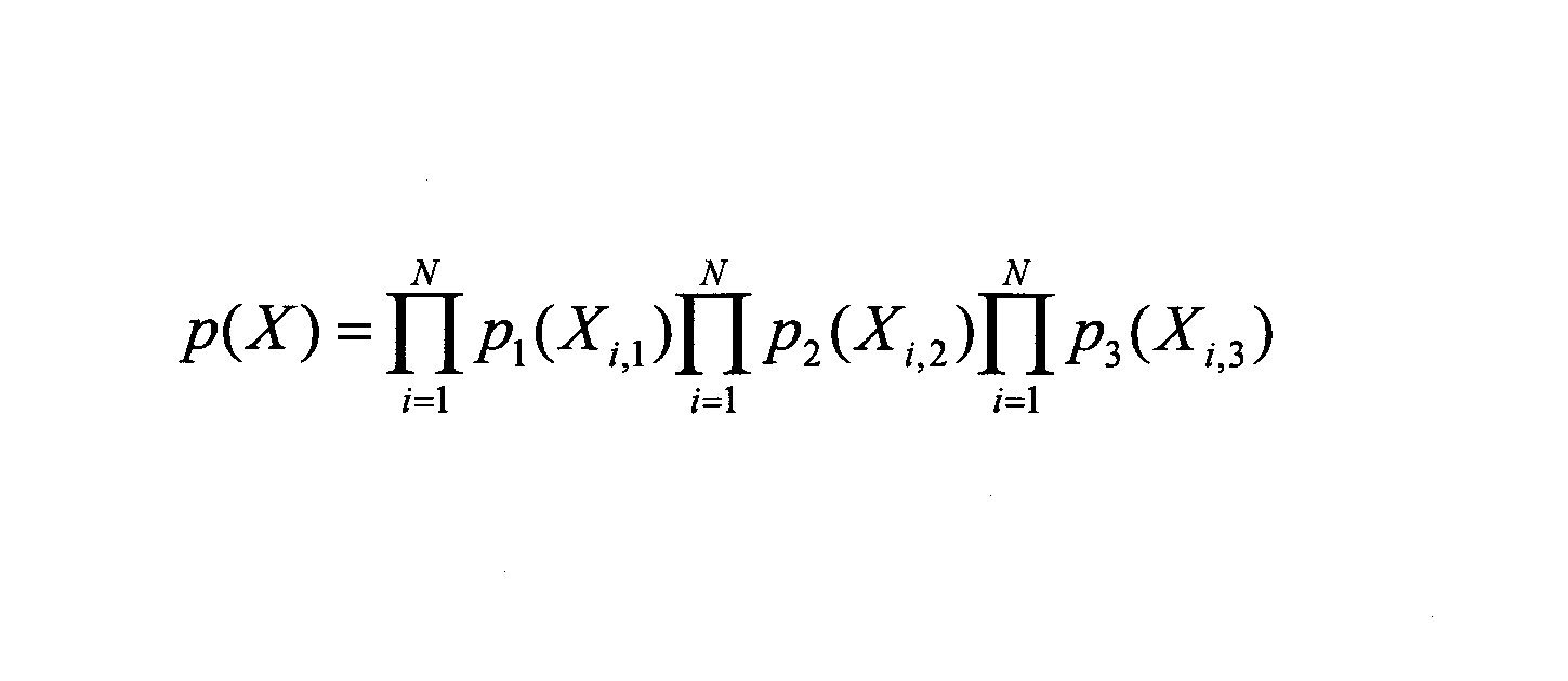
同様に、Xが、q1(x)、q2(x)、q3(x)から発生する確率p(X)は、
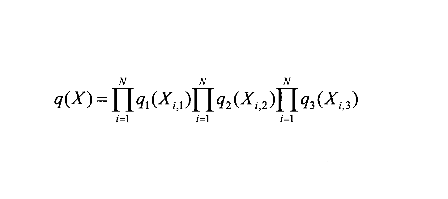
第2の実施の形態において、シミュレーション部11は、N'個のXを生成し、1つのXにつき確率密度関数q1(x)、q2(x)、q3(x)からN個ずつサンプリングする。すなわち、図5のS103において、サンプリング元は、q1(x)、q2(x)、q3(x)である。また、ステップS106においては、dがN'に到達したか否かが判定される。なお、N'<<Mである。
図9のステップS301では、N個ごとにLTBmaxが取得される。したがって、N'個のLTBmaxが取得される。
シミュレーション部11は、ステップS302及びS303の代わりに、以下を実行する。図12は、第2の実施の形態における上側αパーセント点の計算方法を示す図である。
まず、シミュレーション部11は、各Xk(k=1,・・・,N')について、重みWkを以下のように算出する。
Wk=p(Xk)/(q(Xk)×N')
図12の(1)に、Wkの算出結果の一例が示されている。
Wk=p(Xk)/(q(Xk)×N')
図12の(1)に、Wkの算出結果の一例が示されている。
続いて、シミュレーション部11は、N'個のLTBmaxとWkとの組を、LTBmaxの降順にソートする。図12の(2)に、ソート結果の一例が示されている。
続いて、シミュレーション部11は、ソート後のLTBmaxを、yl(l=1,・・・,N')とし、重みWkの累積値である累積重みGl(l=1,・・・,N')を算出する。図12の(2)には、累積重みGlの算出結果の一例が示されている。
ここで、累積重みGlが、α/100以下で、かつ、Glが最大となるlをlαとすると、LTBmaxの上側αパーセント点は、以下の式によって算出することができる。
なお、上記各実施の形態において、シミュレーション部11は、第1の算出部の一例である。在庫量算出部13は、第2の算出部の一例である。ボトルネック工程は、所定の工程の一例である。LTBは、所要時間の一例である。LTBmaxは、所要時間の最大値の一例である。上側αパーセント点は、「上側確率が所定値」の一例である。
以上、本発明の実施例について詳述したが、本発明は斯かる特定の実施形態に限定されるものではなく、請求の範囲に記載された本発明の要旨の範囲内において、種々の変形・変更が可能である。
10 在庫量算出装置
11 シミュレーション部
12 分布推定部
13 在庫量算出部
14 出力部
15 シミュレーションモデル記憶部
16 処理時間分布記憶部
100 ドライブ装置
101 記録媒体
102 補助記憶装置
103 メモリ装置
104 CPU
105 インタフェース装置
B バス
11 シミュレーション部
12 分布推定部
13 在庫量算出部
14 出力部
15 シミュレーションモデル記憶部
16 処理時間分布記憶部
100 ドライブ装置
101 記録媒体
102 補助記憶装置
103 メモリ装置
104 CPU
105 インタフェース装置
B バス
Claims (12)
- 生産ラインにおける所定の工程の前に行われる複数の工程のそれぞれの処理時間の確率分布に基づいて、前記生産ラインの最初の工程から前記所定の工程の前までの処理の所要時間を、複数の材料のそれぞれについて算出する第1の算出部と、
前記複数の材料に関して算出された前記所要時間の分布と、前記所定の工程の処理時間とに基づいて、前記複数の工程における仕掛かり在庫量を算出する第2の算出部と、
を有することを特徴とする在庫量算出装置。 - 前記第2の算出部は、前記所要時間の分布において上側確率が所定値となる所要時間を前記所定の工程の処理時間で除することで、前記在庫量を算出する、
ことを特徴とする請求項1記載の在庫量算出装置。 - 前記第1の算出部は、前記複数の材料のそれぞれについての前記所要時間の算出を複数回繰り返し、
前記第2の算出部は、前記複数回のそれぞれの回における前記所要時間の最大値の分布と、前記所定の工程の処理時間とに基づいて、前記在庫量を算出する、
ことを特徴とする請求項1又は2記載の在庫量算出装置。 - 前記第1の算出部は、少なくとも前記複数の工程のうちの最後の工程と前記所定の工程との間に前記材料の在庫を置くことが可能であるという制約において、前記所要時間を算出する、
ことを特徴とする請求項1乃至3いずれか一項記載の在庫量算出装置。 - 生産ラインにおける所定の工程の前に行われる複数の工程のそれぞれの処理時間の確率分布に基づいて、前記生産ラインの最初の工程から前記所定の工程の前までの処理の所要時間を、複数の材料のそれぞれについて算出し、
前記複数の材料に関して算出された前記所要時間の分布にと、前記所定の工程の処理時とに基づいて、前記複数の工程における仕掛かり在庫量を算出する、
処理をコンピュータが実行することを特徴とする在庫量算出方法。 - 前記所要時間の分布において上側確率が所定値となる所要時間を前記所定の工程の処理時間で除することで、前記在庫量を算出する、
ことを特徴とする請求項5記載の在庫量算出方法。 - 前記複数の材料のそれぞれについての前記所要時間の算出を複数回繰り返し、
前記複数回のそれぞれの回における前記所要時間の最大値の分布にと、前記所定の工程の処理時間とに基づいて、前記複数の工程における仕掛かり在庫量を算出する、
ことを特徴とする請求項5又は6記載の在庫量算出方法。 - 少なくとも前記複数の工程のうちの最後の工程と前記所定の工程との間に前記材料の在庫を置くことが可能であるという制約において、前記所要時間を算出する、
ことを特徴とする請求項5乃至7いずれか一項記載の在庫量算出方法。 - 生産ラインにおける所定の工程の前に行われる複数の工程のそれぞれの処理時間の確率分布に基づいて、前記生産ラインの最初の工程から前記所定の工程の前までの処理の所要時間を、複数の材料のそれぞれについて算出し、
前記複数の材料に関して算出された前記所要時間の分布にと、前記所定の工程の処理時とに基づいて、前記複数の工程における仕掛かり在庫量を算出する、
処理をコンピュータに実行させることを特徴とするプログラム。 - 前記所要時間の分布において上側確率が所定値となる所要時間を前記所定の工程の処理時間で除することで、前記在庫量を算出する、
ことを特徴とする請求項9記載のプログラム。 - 前記複数の材料のそれぞれについての前記所要時間の算出を複数回繰り返し、
前記複数回のそれぞれの回における前記所要時間の最大値の分布にと、前記所定の工程の処理時間とに基づいて、前記複数の工程における仕掛かり在庫量を算出する、
ことを特徴とする請求項9又は10記載のプログラム。 - 少なくとも前記複数の工程のうちの最後の工程と前記所定の工程との間に前記材料の在庫を置くことが可能であるという制約において、前記所要時間を算出する、
ことを特徴とする請求項9乃至11いずれか一項記載のプログラム。
Priority Applications (2)
| Application Number | Priority Date | Filing Date | Title |
|---|---|---|---|
| PCT/JP2016/062231 WO2017183076A1 (ja) | 2016-04-18 | 2016-04-18 | 在庫量算出装置、在庫量算出方法、及びプログラム |
| JP2018512654A JP6597890B2 (ja) | 2016-04-18 | 2016-04-18 | 在庫量算出装置、在庫量算出方法、及びプログラム |
Applications Claiming Priority (1)
| Application Number | Priority Date | Filing Date | Title |
|---|---|---|---|
| PCT/JP2016/062231 WO2017183076A1 (ja) | 2016-04-18 | 2016-04-18 | 在庫量算出装置、在庫量算出方法、及びプログラム |
Publications (1)
| Publication Number | Publication Date |
|---|---|
| WO2017183076A1 true WO2017183076A1 (ja) | 2017-10-26 |
Family
ID=60115795
Family Applications (1)
| Application Number | Title | Priority Date | Filing Date |
|---|---|---|---|
| PCT/JP2016/062231 Ceased WO2017183076A1 (ja) | 2016-04-18 | 2016-04-18 | 在庫量算出装置、在庫量算出方法、及びプログラム |
Country Status (2)
| Country | Link |
|---|---|
| JP (1) | JP6597890B2 (ja) |
| WO (1) | WO2017183076A1 (ja) |
Citations (3)
| Publication number | Priority date | Publication date | Assignee | Title |
|---|---|---|---|---|
| US5826040A (en) * | 1992-03-24 | 1998-10-20 | Texas Instruments Incorporated | Method and system for production planning |
| JP2012194832A (ja) * | 2011-03-17 | 2012-10-11 | Kobe Steel Ltd | 在庫管理方法及び在庫管理プログラム、並びに在庫管理装置 |
| JP2016031739A (ja) * | 2014-07-30 | 2016-03-07 | 株式会社東芝 | 生産制御支援装置および生産制御支援方法 |
-
2016
- 2016-04-18 JP JP2018512654A patent/JP6597890B2/ja not_active Expired - Fee Related
- 2016-04-18 WO PCT/JP2016/062231 patent/WO2017183076A1/ja not_active Ceased
Patent Citations (3)
| Publication number | Priority date | Publication date | Assignee | Title |
|---|---|---|---|---|
| US5826040A (en) * | 1992-03-24 | 1998-10-20 | Texas Instruments Incorporated | Method and system for production planning |
| JP2012194832A (ja) * | 2011-03-17 | 2012-10-11 | Kobe Steel Ltd | 在庫管理方法及び在庫管理プログラム、並びに在庫管理装置 |
| JP2016031739A (ja) * | 2014-07-30 | 2016-03-07 | 株式会社東芝 | 生産制御支援装置および生産制御支援方法 |
Also Published As
| Publication number | Publication date |
|---|---|
| JPWO2017183076A1 (ja) | 2018-11-15 |
| JP6597890B2 (ja) | 2019-10-30 |
Similar Documents
| Publication | Publication Date | Title |
|---|---|---|
| US9697471B2 (en) | Device and method for managing plant model | |
| CN110390503B (zh) | 模型训练、配送时间确定的方法和装置、存储介质和电子设备 | |
| EP3504666A1 (en) | Asychronous training of machine learning model | |
| JP6718500B2 (ja) | 生産システムにおける出力効率の最適化 | |
| US8285409B2 (en) | Effective cycle time management employing a multi-horizon model | |
| JP6290029B2 (ja) | 生産制御支援装置、生産制御支援方法およびプログラム | |
| CN111752903A (zh) | 一种数据存储空间可使用时间的预测方法 | |
| CN114816711A (zh) | 批量任务处理方法、装置、计算机设备和存储介质 | |
| CN112947339A (zh) | 一种基于性能指标的半导体生产线动态调度方法 | |
| CN115222149A (zh) | 资源转换参数管理方法、装置、设备及存储介质 | |
| CN107194489A (zh) | 数据预测方法及装置 | |
| US20150081263A1 (en) | Production simulation apparatus and production simulation method | |
| JP2009245043A (ja) | ライン生産管理支援方法および装置 | |
| JP6597890B2 (ja) | 在庫量算出装置、在庫量算出方法、及びプログラム | |
| JP5600693B2 (ja) | クラスタリング装置及び方法及びプログラム | |
| Betts | Calculating target inventory levels for constrained production: A fast simulation-based approximation | |
| KR20230080213A (ko) | 최적 입력 데이터 생성 장치 및 방법 | |
| US20060136328A1 (en) | Method and system for analyzing the risk of a project | |
| CN113850461A (zh) | 生产计划系统 | |
| JP5793228B1 (ja) | 欠陥数予測装置及び欠陥数予測プログラム | |
| CN108804640B (zh) | 基于最大化iv的数据分组方法、装置、储存介质及设备 | |
| CN116386026B (zh) | 点云3d检测模型的训练方法和点云检测方法 | |
| CN107562695B (zh) | 一种配电变压器的负载数据处理方法及装置 | |
| Barbot et al. | Importance sampling for model checking of continuous time markov chains | |
| US20230336425A1 (en) | Band estimation device, band estimation method, and program |
Legal Events
| Date | Code | Title | Description |
|---|---|---|---|
| WWE | Wipo information: entry into national phase |
Ref document number: 2018512654 Country of ref document: JP |
|
| NENP | Non-entry into the national phase |
Ref country code: DE |
|
| 121 | Ep: the epo has been informed by wipo that ep was designated in this application |
Ref document number: 16899350 Country of ref document: EP Kind code of ref document: A1 |
|
| 122 | Ep: pct application non-entry in european phase |
Ref document number: 16899350 Country of ref document: EP Kind code of ref document: A1 |