WO2017133672A1 - Order o (1) algorithm for first-principles calculation of transient current through open quantum systems - Google Patents
Order o (1) algorithm for first-principles calculation of transient current through open quantum systems Download PDFInfo
- Publication number
- WO2017133672A1 WO2017133672A1 PCT/CN2017/072848 CN2017072848W WO2017133672A1 WO 2017133672 A1 WO2017133672 A1 WO 2017133672A1 CN 2017072848 W CN2017072848 W CN 2017072848W WO 2017133672 A1 WO2017133672 A1 WO 2017133672A1
- Authority
- WO
- WIPO (PCT)
- Prior art keywords
- algorithm
- time
- transient current
- calculation
- transient
- Prior art date
- Legal status (The legal status is an assumption and is not a legal conclusion. Google has not performed a legal analysis and makes no representation as to the accuracy of the status listed.)
- Ceased
Links
Images
Classifications
-
- G—PHYSICS
- G01—MEASURING; TESTING
- G01R—MEASURING ELECTRIC VARIABLES; MEASURING MAGNETIC VARIABLES
- G01R19/00—Arrangements for measuring currents or voltages or for indicating presence or sign thereof
- G01R19/25—Arrangements for measuring currents or voltages or for indicating presence or sign thereof using digital measurement techniques
- G01R19/2506—Arrangements for conditioning or analysing measured signals, e.g. for indicating peak values ; Details concerning sampling, digitizing or waveform capturing
-
- G—PHYSICS
- G01—MEASURING; TESTING
- G01R—MEASURING ELECTRIC VARIABLES; MEASURING MAGNETIC VARIABLES
- G01R31/00—Arrangements for testing electric properties; Arrangements for locating electric faults; Arrangements for electrical testing characterised by what is being tested not provided for elsewhere
- G01R31/28—Testing of electronic circuits, e.g. by signal tracer
- G01R31/317—Testing of digital circuits
- G01R31/31702—Testing digital circuits including elements other than semiconductor transistors, e.g. biochips, nanofabrics, mems, chips with magnetic elements
-
- G—PHYSICS
- G01—MEASURING; TESTING
- G01R—MEASURING ELECTRIC VARIABLES; MEASURING MAGNETIC VARIABLES
- G01R19/00—Arrangements for measuring currents or voltages or for indicating presence or sign thereof
- G01R19/0046—Arrangements for measuring currents or voltages or for indicating presence or sign thereof characterised by a specific application or detail not covered by any other subgroup of G01R19/00
- G01R19/0053—Noise discrimination; Analog sampling; Measuring transients
-
- G—PHYSICS
- G01—MEASURING; TESTING
- G01R—MEASURING ELECTRIC VARIABLES; MEASURING MAGNETIC VARIABLES
- G01R19/00—Arrangements for measuring currents or voltages or for indicating presence or sign thereof
- G01R19/04—Measuring peak values or amplitude or envelope of AC or of pulses
-
- B—PERFORMING OPERATIONS; TRANSPORTING
- B82—NANOTECHNOLOGY
- B82Y—SPECIFIC USES OR APPLICATIONS OF NANOSTRUCTURES; MEASUREMENT OR ANALYSIS OF NANOSTRUCTURES; MANUFACTURE OR TREATMENT OF NANOSTRUCTURES
- B82Y10/00—Nanotechnology for information processing, storage or transmission, e.g. quantum computing or single electron logic
-
- B—PERFORMING OPERATIONS; TRANSPORTING
- B82—NANOTECHNOLOGY
- B82Y—SPECIFIC USES OR APPLICATIONS OF NANOSTRUCTURES; MEASUREMENT OR ANALYSIS OF NANOSTRUCTURES; MANUFACTURE OR TREATMENT OF NANOSTRUCTURES
- B82Y35/00—Methods or apparatus for measurement or analysis of nanostructures
-
- Y—GENERAL TAGGING OF NEW TECHNOLOGICAL DEVELOPMENTS; GENERAL TAGGING OF CROSS-SECTIONAL TECHNOLOGIES SPANNING OVER SEVERAL SECTIONS OF THE IPC; TECHNICAL SUBJECTS COVERED BY FORMER USPC CROSS-REFERENCE ART COLLECTIONS [XRACs] AND DIGESTS
- Y10—TECHNICAL SUBJECTS COVERED BY FORMER USPC
- Y10S—TECHNICAL SUBJECTS COVERED BY FORMER USPC CROSS-REFERENCE ART COLLECTIONS [XRACs] AND DIGESTS
- Y10S977/00—Nanotechnology
- Y10S977/70—Nanostructure
- Y10S977/734—Fullerenes, i.e. graphene-based structures, such as nanohorns, nanococoons, nanoscrolls or fullerene-like structures, e.g. WS2 or MoS2 chalcogenide nanotubes, planar C3N4, etc.
-
- Y—GENERAL TAGGING OF NEW TECHNOLOGICAL DEVELOPMENTS; GENERAL TAGGING OF CROSS-SECTIONAL TECHNOLOGIES SPANNING OVER SEVERAL SECTIONS OF THE IPC; TECHNICAL SUBJECTS COVERED BY FORMER USPC CROSS-REFERENCE ART COLLECTIONS [XRACs] AND DIGESTS
- Y10—TECHNICAL SUBJECTS COVERED BY FORMER USPC
- Y10S—TECHNICAL SUBJECTS COVERED BY FORMER USPC CROSS-REFERENCE ART COLLECTIONS [XRACs] AND DIGESTS
- Y10S977/00—Nanotechnology
- Y10S977/84—Manufacture, treatment, or detection of nanostructure
- Y10S977/842—Manufacture, treatment, or detection of nanostructure for carbon nanotubes or fullerenes
-
- Y—GENERAL TAGGING OF NEW TECHNOLOGICAL DEVELOPMENTS; GENERAL TAGGING OF CROSS-SECTIONAL TECHNOLOGIES SPANNING OVER SEVERAL SECTIONS OF THE IPC; TECHNICAL SUBJECTS COVERED BY FORMER USPC CROSS-REFERENCE ART COLLECTIONS [XRACs] AND DIGESTS
- Y10—TECHNICAL SUBJECTS COVERED BY FORMER USPC
- Y10S—TECHNICAL SUBJECTS COVERED BY FORMER USPC CROSS-REFERENCE ART COLLECTIONS [XRACs] AND DIGESTS
- Y10S977/00—Nanotechnology
- Y10S977/84—Manufacture, treatment, or detection of nanostructure
- Y10S977/88—Manufacture, treatment, or detection of nanostructure with arrangement, process, or apparatus for testing
-
- Y—GENERAL TAGGING OF NEW TECHNOLOGICAL DEVELOPMENTS; GENERAL TAGGING OF CROSS-SECTIONAL TECHNOLOGIES SPANNING OVER SEVERAL SECTIONS OF THE IPC; TECHNICAL SUBJECTS COVERED BY FORMER USPC CROSS-REFERENCE ART COLLECTIONS [XRACs] AND DIGESTS
- Y10—TECHNICAL SUBJECTS COVERED BY FORMER USPC
- Y10S—TECHNICAL SUBJECTS COVERED BY FORMER USPC CROSS-REFERENCE ART COLLECTIONS [XRACs] AND DIGESTS
- Y10S977/00—Nanotechnology
- Y10S977/902—Specified use of nanostructure
- Y10S977/932—Specified use of nanostructure for electronic or optoelectronic application
- Y10S977/936—Specified use of nanostructure for electronic or optoelectronic application in a transistor or 3-terminal device
Definitions
- This invention relates to a transient current calculation as part of the study of the response time and peak transient current in the design of nano-chips in nano electronics.
- Stefanucci et al Phys. Rev. B 77, 075339 (2008) (hereinafter “Stefanucci” ) ; Y. Zhu et al., Phys. Rev. B 71, 075317 (2005) ; J. Maciejko et al., Phys. Rev. B 74, 085324 (2006) (hereinafter “Maciejko” ) ; R. Tuovinen et al., Phys. Rev. B 89, 085131 (2014) (herein after “Tuovinen” ) ; R. Seoane Souto et al., Phys. Rev. B 92, 125435 (2015) and X.
- a novel algorithm based on NEGF-CAP formalism is used to calculate transient current as a function of time step T.
- the computational time of this algorithm is independent of T as long as T ⁇ N 2 where N is the system size.
- the algorithm is order O (1) as long as T ⁇ N 2 .
- transient current based on a non-equilibrium Green’s function (NEGF) that goes beyond the wideband limit (WBL) ; (2) the use of complex absorbing potential (CAP) so that the transient current can be expressed in terms of poles of Green’s function; (3) within the NEGF-CAP formalism the transient current can be calculated separately in the space and time domains making the O (1) algorithm possible so that at this point the computational complexity reduces to 50N 3 +TN 2 (algorithm I) ; and (4) the exploitation of a Vandermonde matrix enables the use of the fast multipole method (FMM) and fast Fourier transform (FFT) to further reduce the scaling to 50N 3 +2N 2 log 2 N for T ⁇ N 2 and large N, which is therefore completely independent of T (algorithm II) .
- FMM fast multipole method
- FFT fast Fourier transform
- Every physical phenomena in a real device can be accurately calculated and predicted once its composition is known, e.g., how many atoms, which types of atoms, etc.
- the algorithm of the present invention to calculate and predict the actual response of a nano-device.
- This fast algorithm makes the computational complexity of transient current calculation comparable to that of a static calculation.
- the huge speed gain enables the performance of first principles transient calculations and nano-device design on a modest computer workstation.
- the Hamiltonian (the operator corresponding to the total energy of the system in most of the cases) is given by
- (c) denotes the electron creation (annihilation) operator in the lead region.
- the second and third terms represent the Hamiltonian in the central scattering region and its coupling to leads, respectively.
- the time-dependent Coulomb interaction U n (t) in the scattering region This Hamiltonian can be obtained using the first-principle method or it can be assumed to be a tight-binding form. Taking the time-dependent terminal current I ⁇ (t) of lead ⁇ is defined as in the Zhang article.
- the upward step-like bias pulse the A ⁇ ( ⁇ , t) is found in the Maciejko article to be
- ⁇ ⁇ is the amplitude of the external bias-V ⁇
- G ⁇ in Eq. (1) is the lesser Green’s function of the central scattering region excluding the CAP regions. Substituting the second term of Eq. (4) into the first term in Eq. (1) , its contribution to current (denoted as I 1 ) is
- I 0L is the long time limit of the transient current which can be calculated using the Landauer Buttiker formula.
- the time dependent part of the transient current can be separated into a real space calculation (calculation of M 1 and M 2 ⁇ ) and then a matrix multiplication involving time.
- the Fermi function can be accurately approximated by 15 or 20 Pade approximants.
- the calculation of can be combined to give TN 2 computational complexity.
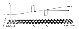
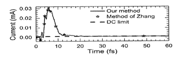
- FIG. 1A shows the configuration of a gated graphene nanoribbon and a voltage applied to it over time and FIG. 1B shows the transient current of the zigzag graphene nanoribbon for a system of 600 atoms for the present invention and the Zhang method ;
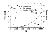
- FIG. 2 shows the scaling of computation time versus the number of computations N for the prior art Zhang method and the Algorithm I of the method according to the present invention
- FIG. 4 shows a graph of the typical behavior of transient current, wherein the inset is the long time behavior between 17ps to 18ps;
- FIG. 5 is a graph of the transmission coefficient of a zigzag graphene nanoribbon for a system of 10,000 atoms calculated by 30 layers of CAP and by exact numerical solution;
- FIG. 6 shows the distribution of (1/ ⁇ T ) j on the complex plane
- FIG. 7 shows the distribution of d j on the complex plane
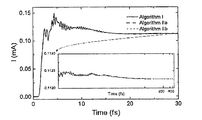
- FIG. 8 illustrates the transient current calculated by Algorithm I, Algorithm IIa and Algorithm IIb.
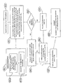
- FIG. 9 is a flow chart showing the process for the calculation of the algorithm according to the present invention.
- transient current calculation is essential to the study of the response time and to capture the peak transient current for preventing the melt down of nano-chips in nano-electronics.
- T For a period of time T, its calculation is known to be extremely time consuming with the best scaling being TN 3 where N is the dimension of the device.
- the dynamical response of the system is usually probed by sending a step-like pulse and monitoring its transient behavior.
- the present invention is directed to a new algorithm for calculating the transient current of a system, which requires much less computational time than the prior art.
- FIG. 9 shows a flow chart of the method for calculating the algorithm of the present invention. It can be carried out on a computer workstation as part of the design of a nano-device.
- the algorithm provides an O (1) computational method for obtaining the transient response of current I (t) over the entire user-defined time period under suitable conditions.
- the input parameters for this algorithm include Hamiltonians of the open quantum system before and after the transient process denoted as H eq and H neq ⁇ These Hamiltonians, whether based on atomistic first-principle density functional theory (DFT) or tight-binding methods, can be adopted at will for the system of interest. Nonetheless, complex absorbing potential (CAP) is required to represent the self-energy of the leads of the device. Subsequently, corresponding eigenstate and energy can be generated and fed into the algorithm. Additionally, Fermi function is expanded using Pade spectrum decomposition (PSD) .
- PSD Pade spectrum decomposition
- step 901 of FIG. 9 the process begins with input preparation.
- step 901A which involves forming Preliminary Input quantities H eq , H neq (From first-principle (DFT) , TB, etc) and Self energy of leads (from CAP) .
- step 901B eigenstates and eigen-energy are generated. This input information is then directed to step 902.
- step 902 The results of step 902 are then reviewed in step 904 to see if they contain time dependent components. Ifthe answer is NO, the process moves to step 905.
- step 905 the process computes and constructs space dependent matrices by an optimized matrix multiplication process. From step 905 the process goes to step 906 where the FMM and FFT methods are used for computing the multiplication of V m and M n .
- step 904 If the result of step 904 is YES, the process moves to step 907 where Vandermonde matrices are prepared before moving to step 906. The results in both step 905 and 906 are summed in Step 908. The summed results are directed to output step 909, where the complete transient response I (t) over the user-defined time period is generated.
- the algorithm of the present invention was tested on a gated graphene nanoribbon at room temperature using the tight-binding (TB) Hamiltonian given by
- the solid line (T S ) is the exact numerical result using self-energy of the lead and the dashed line (T CAP ) is from CAP. This also ensures the correct steady state current.
- excellent agreement is also obtained between the algorithm of the present invention and that of the Zhang reference (See FIG. 2) .
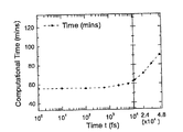
- the scaling is shown in FIG. 3, from which it can be seen that for T ⁇ N the computational time is almost independent of the number of time steps.
- t 1 the CPU time needed for the spacial calculation (50N 3 )
- t 2 is the time needed for the temporal part (matrix multiplication in Eq. (7) ) using, e.g., a Xeon X5650 workstation with 12 cores and a frequency of 2.67 GHz.
- multithreading could be very inefficient so a single core has been used to perform the calculation.
- the fitted curve which is in the form of 50N 3 +TN 2 , is in good agreement with the calculated results
- the Y-axis is on the right.
- 6000 energy points were used for integration using the Y-axis on the left.
- the left hand side uses an exponential scale in t and the right hand side uses a linear scale in t.
- FIG. 3 shows that at extremely large data points, e.g., ranges over 10 thousands points, the computational time is proportional to T.
- the algorithm of the present invention is based on the NEGF-CAP formalism, it can be extended to the NEGF-DFT-CAP formalism which performs the first principles calculation.
- the NEGF-DFT-CAP method has already been successfully implemented in the first principles transient current calculation as shown in the Zhang reference, which gives exactly the same result as that of NEGF-DFT.
- the transient spin current (related to spin transfer torque) using the NEGF-DFT-CAP formalism has been carried out for planar structures where k-sampling in the first Brillouin zone is needed. It is straightforward to include k-sampling in the method of the present invention.
- transient current I R (t) is similar to Eq. (7) .
- FIG. 5 shows the transmission coefficient of the zigzag graphene nanoribbon for a system of 10,000 atoms.
- the solid line (T S ) is the exact numerical result using self-energy of the lead and the dashed line (T CAP ) is from CAP.
- T S the exact numerical result using self-energy of the lead
- T CAP the dashed line
- FIG. 5 shows a comparison between the exact numerical result of the transmission coefficient using the self-energy of the lead and that of CAP. There is very close agreement.
- Eq. (14) is of the form V t MV * where t stands for transpose.
- FMM fast multipole method
- the configuration of the system is the same as that which appears in FIG. 1, except the width W of the system is now 17 times wider with a total of 10200 ⁇ 10 4 atoms. Each time step is 0.012 fs.
- the computed transient current using Algorithm I and II are shown in FIG. 8. The purpose of this calculation is to test the computational complexity only. All that needs to be done is to compute,
- T ⁇ N the results of the algorithm I, the algorithm IIa and the algorithm IIb are on top of each other.
- FIG. 6, only shows the results for T ⁇ 40,000. There is no significant feature in the transient current plot beyond that.
- FIG. 7 shows the distribution of d j on the complex plane.
Landscapes
- Physics & Mathematics (AREA)
- General Physics & Mathematics (AREA)
- Engineering & Computer Science (AREA)
- Chemical & Material Sciences (AREA)
- Nanotechnology (AREA)
- General Engineering & Computer Science (AREA)
- Power Engineering (AREA)
- Superconductor Devices And Manufacturing Methods Thereof (AREA)
- Complex Calculations (AREA)
- Investigating Or Analyzing Materials By The Use Of Electric Means (AREA)
Abstract
A fast algorithm is used to study the transient behavior due to the step-like pulse. This algorithm consists of two parts: The algorithm I reduces the computational complexity to T0N3 for large systems as long as T<N; The algorithm II employs the fast multipole technique and achieves scaling T0N3 whenever T<N2 beyond which it becomes T log2 N for even longer time. Hence it is of order O(1) if T<N2. Benchmark calculation has been done on graphene nanoribbons with N=104 and T=108. This new algorithm allows many large scale transient problems to be solved, including magnetic tunneling junctions and ferroelectric tunneling junctions that could not be achieved before.
Description
This invention relates to a transient current calculation as part of the study of the response time and peak transient current in the design of nano-chips in nano electronics.
At the heart of growing demands for nanotechnology is the need of ultrafast transistors whose response time is one of the key performance indicators. The response of a general quantum open system can be probed by sending a step-like pulse across the system and monitoring its transient current over time, thus making transient dynamics a very important consideration. Many experimental data show that most molecular device characteristics are closely related to the material and chemical details of the device structure. Therefore, first principles analysis, which involves quantitative and predictive analysis of device characteristics, especially their dynamic properties, without relying on any phenomenological parameter, becomes a central interest in the design of nanoelectronics.
The theoretical study of transient current dates back twenty years to when the exact solution in the wideband limit ( “WBL” ) was obtained by Wingreen et al. See, N. S. Wingreen et al., Phys. Rev. B 48, 8487 (R) (1993) , which is incorporated herein by reference in its entirety. Since then transient current has been studied extensively using various methods, including the scattering wave function, non-equilibrium Green’s function ( “NEGF” ) approach, and density matrix method. See, J. Wang, J. Comput. Electron. 12, 343-355 (2013) ; S. Kurth et al., Phys. Rev. B 72, 035308 (2005) (hereinafter “Kurth” ) ; G. Stefanucci et al, Phys. Rev. B 77, 075339 (2008) (hereinafter “Stefanucci” ) ; Y. Zhu et al., Phys. Rev. B 71, 075317 (2005) ; J. Maciejko et al., Phys. Rev. B 74, 085324 (2006) (hereinafter “Maciejko” ) ; R. Tuovinen et al., Phys. Rev. B 89, 085131 (2014) (herein after “Tuovinen” ) ; R. Seoane Souto et al., Phys. Rev. B 92, 125435 (2015) and X. Zheng et al., Phys. Rev. B 75, 195127 (2007) , all of which are incorporated herein by reference. The major obstacle to the theoretical investigation of transient current is its computational complexity. Many attempts
have been made trying to speed up the calculation See Kurth and Tuovinen, as well as L. Zhang et al., Phys. Rev. B 86, 155438 (2012) ; B. Gaury et al., Phys. Rep. 534, 1-37 (2014) ; M. Ridley et al., J. Phys.: Conf. Ser. 696, 012017 (2016) (hereinafter “Ridley” ) ; H A. Croy et al., Phys. Rev. B 80, 245311 (2009) and F J. Weston et al., Phys. Rev. B 93, 134506 (2016) , all of which are incorporated herein by reference in their entirety.
Despite these efforts, the best algorithm for calculating the transient current from first principles going beyond WBL limit scales like TN3 using a complex absorbing potential ( “CAP” ) , where T and N are the number of time steps and the size of the system, respectively. See, L. Zhang et al, Phys. Rev. B 87, 205401 (2013) (hereinafter “Zhang” ) , which is incorporated herein by reference in its entirety. It should be noted that if WBL is used, the scaling is reduced. See, the Ridley article. However, to capture the feature of the band structure of the lead and the interaction between the lead and the scattering region, WBL is not a good approximation in the first principles calculation. As a result, most of the first principles investigations of transient dynamics were limited to small and simple one-dimensional systems.
There are a number of problems, such as with magnetic tunneling junctions (MTJ) and ferroelectric tunneling junctions, where the system is two dimensional or even three dimensional in nature. See, Z. Y. Ning et al., Phys. Rev. Lett. 100, 056803 (2008) and J. D. Burton et al., Phys. Rev. Lett. 106, 157203 (2011) , which are incorporated herein by reference in their entirety. For these systems, a large number of k points Nk have to be sampled in the first Brillouin to capture accurately the band structure of the system. For MTJ structures like Fe-MgO-Fe, at least Nk=104 k points must be used to give a converged transmission coefficient. See, D. Waldron et al., Phys. Rev. Lett. 97, 226802 (2006) , which is incorporated herein by reference in its entirety. This makes the time consuming transient calculation Nk times longer, which is an almost impossible task even with high performance supercomputers. Clearly it is urgent to develop better algorithms to reduce the computational complexity.
Summary of the Invention
According to the present invention a novel algorithm based on NEGF-CAP formalism is used to calculate transient current as a function of time step T. The computational time of this algorithm is independent of T as long as T<N2 where N is the
system size. Hence the algorithm is order O (1) as long as T<N2. Four important factors are essential to achieve this result: (1) the availability of an exact solution of transient current based on a non-equilibrium Green’s function (NEGF) that goes beyond the wideband limit (WBL) ; (2) the use of complex absorbing potential (CAP) so that the transient current can be expressed in terms of poles of Green’s function; (3) within the NEGF-CAP formalism the transient current can be calculated separately in the space and time domains making the O (1) algorithm possible so that at this point the computational complexity reduces to 50N3+TN2 (algorithm I) ; and (4) the exploitation of a Vandermonde matrix enables the use of the fast multipole method (FMM) and fast Fourier transform (FFT) to further reduce the scaling to 50N3+2N2log2 N for T<N2 and large N, which is therefore completely independent of T (algorithm II) . See V. Rokhlin, J. Comput. Phys., 60, 187-207 (1985) (hereinafter “Rokhlin” ) and J. Song et al., IEEE trans. Antennas Propagat. 45, 1488-1493 (1997) (hereinafter “Song” ) , which are both incorporated herein by reference in their entirety. It is possible with this new algorithm to calculate, and thus predict, the actual response of a nano-device theoretically without experimental data. Thus, the algorithm is useful in the design of a nano-device before actual production.
Everything is made of atoms. In theory, every physical phenomena in a real device can be accurately calculated and predicted once its composition is known, e.g., how many atoms, which types of atoms, etc. From the Hamiltonian (a quantity that stores the physical information of the system based on the particular electrons of particular elements present in the devices) , it is possible to use the algorithm of the present invention to calculate and predict the actual response of a nano-device. To verify the computational complexity, benchmark calculations were carried out on graphene nanoribbons using the tight-binding model. A speed up factor of 1000T was gained for a system size of N=2400. A calculation was also done for the same system with N=10, 200 and T=108 confirming the O (1) scaling. This fast algorithm makes the computational complexity of transient current calculation comparable to that of a static calculation. Thus, the huge speed gain enables the performance of first principles transient calculations and nano-device design on a modest computer workstation.
For a general open quantum system with multiple leads under a step-like bias pulse, the Hamiltonian (the operator corresponding to the total energy of the system in most of the cases) is given by

where (c) denotes the electron creation (annihilation) operator in the lead region. The first term in this equation corresponds to the Hamiltonian of leads with
 the energy of lead α which contains external bias voltage vα (t) =Vαθ (±t) .. The second and third terms represent the Hamiltonian in the central scattering region and its coupling to leads, respectively. Also included is the time-dependent Coulomb interaction Un (t) in the scattering region. This Hamiltonian can be obtained using the first-principle method or it can be assumed to be a tight-binding form. Taking
 the time-dependent terminal current Iα (t) of lead α is defined as in the Zhang article.

where is an auxiliary projection matrix which is used for measuring the transient current passing through the lead α. Here G< and H (t) are the lesser Green’s function and the Hamiltonian of the central scattering region, respectively. For a step-like pulse an exact solution for G< has been obtained by Maciejko et al. as described in the Maciejko article, which goes beyond the WBL and has been applied to first principles calculation of transient current for atomic junctions. Next, the case of an upward pulse vα (t) =VαΘ (t) can be considered. In order to have an exact solution as described in the Maciejko article, it is assumed that Un (t) =Un, eq+ (Un, neq-Un, eq) Θ (t) where Un, eq is the equilibrium Coulomb potential, while Un, neq is the non-equilibrium potential at a long time limit. Note that the fast algorithm relies on this approximation where the self-consistent Coulomb potentials are needed only at two points: t=0- and t=∞. As a result of this approximation, at t=0, the system is in equilibrium with Hamiltonian Heq while at t>0 the system is in a non-equilibrium state with a time-independent Hamiltonian Hneq. In terms of a spectral function Aα (ε, t) , the lesser Green’s function G< is given by the Maciejko article as

The upward step-like bias pulse the Aα (ε, t) is found in the Maciejko article to be

where and
and are the non-equilibrium and equilibrium retarded Green functions, respectively, Δα is the amplitude of the external bias-Vα, and Δ=Uneq-Ueqis a matrix where the subscript “neq” and “eq” refer to non-equilibrium and equilibrium potentials, respectively.
Despite the simplification from the conventional double time G< (t, t') to single time G< (t, t) used in Eq. (1) , the computational cost to obtain G< remains very demanding for the following reasons:
(1) Consider Aα (ε, t) with a matrix size of N, matrix multiplications  and
and in the integrand of Eq. (3) require computational complexity of O (N3) for each time step. As a result, the total computational cost over a period of time is at least O (TN3) where T is the number of time steps.
(2) Double integrations in energy space are required for G<. The presence of numerous quasi-resonant states whose energies are close to the real energy axis makes the energy integration in Aαextremely difficult to converge.
This problem can be overcome using the CAP method as described in the article J. Driscoll and K. Varga, Phys. Rev. B 78, 245118 (2008) , which is incorporated herein by reference in its entirety. The essence of the CAP method is to replace each semi-infinite lead by a finite region of CAP while keeping the transmission coefficient of the system
unchanged. In addition, it is demonstrated in the Zhang article that the first principles result of transient current for molecular junctions obtained from the exact numerical method (non-WBL) and the CAP method are exactly the same. Using the CAP method, the poles of Green’s function can be obtained easily and the spectral function can be calculated analytically using the residue theorem. Expanding the Fermi function using the Pade spectrum decomposition (PSD) , as explained more fully in the detailed description of the invention below, further allows for the calculation of the transient current separately in space and time domain making the O (T0N3) algorithm possible. See, J. Hu et al., J. Chem. Phys. 133, 101106 (2010) , which is incorporated herein by reference in its entirety.
Achieving the algorithm of the present invention for the transient current calculation can now be demonstrated, i.e., Iα (tj) for j=1, 2, ..., T. First Eq. (3) is substituted into Eq. (2) , and G< (t, t) can be written as

where,


where εn and εm (n=1, 2, ...N) is the complex energy spectrum of in the lower half plane,
  are the poles of f (E) using PSD with l=1, ...Nf ; and Nfis the total number of those poles for the adopted Pade approximant.
Within the CAP framework, G< in Eq. (1) is the lesser Green’s function of the central scattering region excluding the CAP regions. Substituting the second term of Eq. (4) into the first term in Eq. (1) , its contribution to current (denoted as I1) is

where the matrix M does not depend on time. Thus, the space and time domains have been separated.
Denoting a Vandermonde matrix Vjk=exp (iεktj) with k=1, 2, ..., N, tj=jdt, j=1, 2, ..., T where dt is the time interval and Using this approach, IL is finally obtained. This calculation is more fully explained in the detailed description below.

where is a T×Nfmatrix, M1 is a N×N matrix while M2 is a N×Nfmatrix. Since εkis the complex energy in the lower half plane, Vjkgoes to zero at large j. Hence I0L is the long time limit of the transient current which can be calculated using the Landauer Buttiker formula. The time dependent part of the transient current can be separated into a real space calculation (calculation of M1 and M2α) and then a matrix multiplication involving time. At room temperatures the Fermi function can be accurately approximated by 15 or 20 Pade approximants. Hence the calculation of
  can be combined to give TN2 computational complexity.
The computational complexity of this algorithm (denoted as algorithm I) can now be examined. By counting the number of matrix multiplication, the computational complexity of the real space calculations can be estimated to be 50N3. Therefore the total computational complexity is 50N3+TN2. At this stage, the algorithm is not O (1) yet. In the detailed description below it is shown that matrix multiplication VtM, where M is M1 or M2α, can be done using the FMM and FFT (denoted as algorithm II) . This reduces the computational complexity of VtM from TN2to Tlog2N. Hence for T<N2, the computational complexity is 50N3+N2log2N. For T>N2, the scaling is 50N3+Tlog2N. However, for large T, the physics comes into play. Since εj is the complex energy of the resonant state, VjT=exp (-iεjdtT) decays quickly to zero before T=N2. For a graphene nanoribbon with N=104 (see details below) , the maximum value of VjT=exp (-iεjdtT) is 10-3when T=N and dt=1 fs. Consequently all of the matrix elements are zero for T=10N. Hence for large systems, the chance to go beyond T=N2is small. In this sense, algorithm II is an order O (1) algorithm.
The foregoing and other objects and advantages of the present invention will become more apparent when considered in connection with the following detailed description and appended drawings in which like designations denote like elements in the various views, and wherein:
FIG. 1A shows the configuration of a gated graphene nanoribbon and a voltage applied to it over time and FIG. 1B shows the transient current of the zigzag graphene nanoribbon for a system of 600 atoms for the present invention and the Zhang method;
FIG. 2 shows the scaling of computation time versus the number of computations N for the prior art Zhang method and the Algorithm I of the method according to the present invention;
FIG. 3 shows the scaling of computational time against time t for N equal to 10,200, time step dt=1 fs;
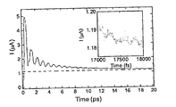
FIG. 4 shows a graph of the typical behavior of transient current, wherein the inset is the long time behavior between 17ps to 18ps;
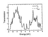
FIG. 5 is a graph of the transmission coefficient of a zigzag graphene nanoribbon for a system of 10,000 atoms calculated by 30 layers of CAP and by exact numerical solution;
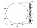
FIG. 6 shows the distribution of (1/ωT) jon the complex plane;
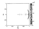
FIG. 7 shows the distribution of djon the complex plane;
FIG. 8 illustrates the transient current calculated by Algorithm I, Algorithm IIa and Algorithm IIb; and
FIG. 9 is a flow chart showing the process for the calculation of the algorithm according to the present invention.
Detailed Description of Exemplary Embodiments
First principles transient current calculation is essential to the study of the response time and to capture the peak transient current for preventing the melt down of nano-chips in nano-electronics. For a period of time T, its calculation is known to be extremely time consuming with the best scaling being TN3where N is the dimension of the device. The dynamical response of the system is usually probed by sending a step-like pulse and monitoring its transient behavior.
The present invention is directed to a new algorithm for calculating the transient current of a system, which requires much less computational time than the prior art. FIG. 9 shows a flow chart of the method for calculating the algorithm of the present invention. It can be carried out on a computer workstation as part of the design of a nano-device.
Generally speaking, the algorithm provides an O (1) computational method for obtaining the transient response of current I (t) over the entire user-defined time period under suitable conditions. The input parameters for this algorithm include Hamiltonians of the open quantum system before and after the transient process denoted as Heq and Hneq·These Hamiltonians, whether based on atomistic first-principle density functional theory (DFT) or
tight-binding methods, can be adopted at will for the system of interest. Nonetheless, complex absorbing potential (CAP) is required to represent the self-energy of the leads of the device. Subsequently, corresponding eigenstate and energy can be generated and fed into the algorithm. Additionally, Fermi function is expanded using Pade spectrum decomposition (PSD) .
It is only possible to construct the particular exact equation of transient current which can be calculated separated in space and time domains by using the mentioned form of input ingredients. Once such an equation is constructed, whether for the case for step-up, step-down bias or other similar classes of transient response, so that I (t) is a function of Io, Vm (t) and Mn for some m and n where Vm (t) are Vandemonde matrices and Io and Mn are time independent matrices. Once the required Vandemonde matrices and Mn are constructed, fast multi pole method (FMM) and fast Fourier transform (FFT) are used to calculate the matrix multiplication between them. Eventually, I (t) can be obtained by summing up the contribution due to Io, Vm (t) and Mn.
In step 901 of FIG. 9 the process begins with input preparation. This includes step 901A, which involves forming Preliminary Input quantities Heq, Hneq (From first-principle (DFT) , TB, etc) and Self energy of leads (from CAP) . In step 901B eigenstates and eigen-energy are generated. This input information is then directed to step 902. In step 902 construction is performed on the exact equation of transient current based on NEGF formalism that is organized into the general form of I (t) =lt (Io, Vm (t) , Mn) such that it is a function composed of time dependent Vandermonde matrices Vm and other space dependent matrices Mn. Also, there is an input from step 903, i.e., Fermi functions (from the PSD method) to step 902.
The results of step 902 are then reviewed in step 904 to see if they contain time dependent components. Ifthe answer is NO, the process moves to step 905. In step 905 the process computes and constructs space dependent matrices by an optimized matrix multiplication process. From step 905 the process goes to step 906 where the FMM and FFT methods are used for computing the multiplication of Vm and Mn.
If the result of step 904 is YES, the process moves to step 907 where Vandermonde matrices are prepared before moving to step 906. The results in both step 905
and 906 are summed in Step 908. The summed results are directed to output step 909, where the complete transient response I (t) over the user-defined time period is generated.
To demonstrate the power of the algorithm according to the present invention, the transient current in a graphene nanoribbon is calculated. Graphene is a well-known intrinsic 2D material with many exotic properties. See, A. H. Castro Neto et al., Rev. Mod. Phys. 81, 109 (2009) and Y. Zhang et al., Nature, 438, 201-204 (2005) , which are incorporated herein by reference in their entirety. Studies of its transient behavior in response to a step-like pulse have been reported in the literature. See the Stefanucci article and E. Perfetto et al., Phys. Rev. B 82, 035446 (2010) and Y. O. Klymenko et al., Eur. Phys. J. B 69, 383-388 (2009) , which are both incorporated herein by reference in their entirety.
The algorithm of the present invention was tested on a gated graphene nanoribbon at room temperature using the tight-binding (TB) Hamiltonian given by

where is the creation (annihilation) operator at site i and h0=2.7eV being the nearest hopping constant. Here V (x) =VL+ (VR-VL) x/L is the potential landscape due to the external bias with VR=-VL=0.54V, and Vg1 and Vg2being the gate voltages in regions S1 and S2, respectively.
First it is confirmed that the transient current calculated using the new method is the same as that of the Zhang reference. Using 30 layers of CAP, the transmission coefficient versus the energy was calculated and it showed good agreement with the exact solution. FIG. 5 provides a comparison for a graphene nanoribbon with N=10,000. In FIG. 5 the solid line (TS) is the exact numerical result using self-energy of the lead and the dashed line (TCAP) is from CAP. This also ensures the correct steady state current. For the transient current, excellent agreement is also obtained between the algorithm of the present invention and that of the Zhang reference (See FIG. 2) . It should be noted that in the presence of gates, the “on-off” time of graphene is shortened in comparison to un-gated graphene which has a long oscillating current as reported in the Stefannucci article. Also the transient current is
calculated for a graphene nanoribbon with size of N=104and T=20,000 with each time step 1fs. See FIG. 5.
Now testing of the scaling of the algorithm of the present invention can be achieved by calculating the transient current for nanoribbons with different system sizes ranging from 600 to 10,200 atoms. The first test is with algorithm I. The computational time for the transient current for 3 time steps compared against system sizes N is shown in FIG. 2. In FIG. 5 the data is fitted using 50N3+TN2with very good agreement showing TN2 scaling for the time-dependent part. For comparison, FIG. 5 also shows a plot of the computation time using the method in the Zhang reference. It was found that the number of energy points NEdepends on the spectrum of resonant states of the system. For graphene nanoribbons with 600 atoms, NE=6000 was used to converge the integral over a Fermi function. FIG. 2 shows that a speed up factor of 1000T is achieved at N=2400. The scaling is shown in FIG. 3, from which it can be seen that for T<N the computational time is almost independent of the number of time steps.
Now algorithm II, which reduces the scaling TN2further, can be examined. Notice that the scaling TN2comes from matrix multiplication involving Vandermonde matrix VtM1. The fast algorithm is available to speed up the calculation involving a structured matrix, such as the Vandermonde matrix. As discussed in detail below the FMM as in the Rokhlin and Song articles and FFT can be used to carry out the same matrix multiplication using only c3N2log2N operations provided that T<N2. Here the coefficient c3 is a large constant that depends only on the tolerance of the calculation τ and the setup of FMM. The theoretical estimate of this coefficient is about 40log2 (1/τ) where τ is the tolerance in the FMM calculation, which used τ=10-4. See N. Yarvin et al., Anal. 36, 629 (1999) , which is incorporated herein by reference in its entirety. When implementing FMM, this coefficient is in general larger than the theoretical one.
To test algorithm II, the transient current is calculated for N=104and T=108 as explained in detail below, using FMM and FFT. Denote t1 the CPU time needed for the
spacial calculation (50N3) , t2is the time needed for the temporal part (matrix multiplication in Eq. (7) ) using, e.g., a Xeon X5650 workstation with 12 cores and a frequency of 2.67 GHz. The result t1=3500s is obtained using 12 cores and t1=33800s using a single core so the efficiency of multithreading is about 80%. For an FMM calculation, multithreading could be very inefficient so a single core has been used to perform the calculation. It was found t2=3400s for T=108 using a single core, as shown below in the detailed computational analysis and numerical calculation. It was found that for T=108the time spent in the time dependent part is about one tenth of the time of the independent calculation. This confirms that the method of the present invention uses an algorithm of order O (1) as long as T<N2. It should be pointed out that algorithm II is directed to the calculation of the transient current I (t) with time steps T=N2at one shot with scaling N2log2N. This scaling remains if I (t) with the number of time step less than N2is desired.
FIG. 2 shows the scaling of N against computation time at T=3 (each time step is 1fs) . The fitted curve, which is in the form of 50N3+TN2, is in good agreement with the calculated results The Y-axis is on the right. In order compare the present invention to the performance reported in the Zhang reference, 6000 energy points were used for integration using the Y-axis on the left.
FIG. 3 illustrates the scaling of t against CPU time for N=10,200 (t=100 fs corresponds to T=100) using algorithm I. The left hand side uses an exponential scale in t and the right hand side uses a linear scale in t. FIG. 3 shows that at extremely large data points, e.g., ranges over 10 thousands points, the computational time is proportional to T.
Since the algorithm of the present invention is based on the NEGF-CAP formalism, it can be extended to the NEGF-DFT-CAP formalism which performs the first principles calculation. In fact, the NEGF-DFT-CAP method has already been successfully implemented in the first principles transient current calculation as shown in the Zhang reference, which gives exactly the same result as that of NEGF-DFT. With the fast algorithm at hand, many applications can be envisaged. For instance, the transient spin current (related to spin transfer torque) using the NEGF-DFT-CAP formalism has been carried out for planar structures where k-sampling in the first Brillouin zone is needed. It is straightforward to
include k-sampling in the method of the present invention. It is also possible to extend this method to the case where electron-phonon interaction in the Born approximation as well as other dephasing mechanisms are present. Finally, first principles transient photo-induced current on two dimensional layered materials can be calculated using the method of the present invention.
Some of the details of the calculations presented above are given here.
Pade approximant
Brute force integration over the Fermi function along the real energy axis to obtain G< (t, t) may need thousands of energy points to converge, which is very inefficient. To obtain an accurate result while reducing the cost, fast converging Pade spectrum decomposition (PSD) is used for the Fermi function f in Eq. (4) above, so that the residue theorem can be applied. Using [n-1/n] PSD scheme with the Pade approximant accurate up to O ( (ε/kT) 4n-1) , Fermi function f can be expressed as

where ξj and ηjare two set of constants that can be calculated easily. Using the PSD scheme analytic form of G<in Eq. (4) can be obtained using the residue theorem. See J. Hu et al., J. Chem. Phys. 133, 101106 (2010) , which is incorporated herein by reference in its entirety.
Calculation of the spectral function
The terms and
and the equilibrium and non-equilibrium retarded Green’s functions, respectively, can be expressed in terms of their eigen-functions by solving the following eigen-equations for Heq and Hneq, i.e.,


where and similar equations can be defined for Hneq. See the Zhang reference. Using the eigen-functions of Heq-iW and Hneq-iW, we have


Performing an integral over ω using the residue theorem, the analytic solution of Aαis obtained

where Δ=Hneq-Heq.
Calculation of the lesser Green’s function
In Eq. (5) using residue theorem the involved terms are defined as


Calculation of the transient current
Starting from Eq. (1) and in analogue to Eq. (6) , the expressions of the current in Eq. (7) can be obtained as follows:


The expression of transient current IR (t) is similar to Eq. (7) .
Transient current for a graphene nanoribbon of system size N=104
A calculation was performed on transient current through a zigzag graphene nanoribbon of 10,000 atoms with T=20,000 time steps (each time step is 1fs) . The width of the system is two unit cells (16 atoms) while the length of the system is 625 unit cells. Two gate voltages of 2.2V were applied so that the system is in the tunneling regime. The bias voltage is vL=-vR=0.5V. From FIG. 4, it can be seen that a typical behavior of transient current with the current shooting up initially and then decreasing oscillations to the long time limit (the numerical results using FMM show that 100 ps is needed to reach the dc limit,
which is shown as a dashed line) . The oscillatory behavior is due to resonant states in the system. This test was at a temperature of 300°K. The inset is the long time behavior between 17ps to 18ps.
FIG. 5 shows the transmission coefficient of the zigzag graphene nanoribbon for a system of 10,000 atoms. The solid line (TS) is the exact numerical result using self-energy of the lead and the dashed line (TCAP) is from CAP. Thus, FIG. 5 shows a comparison between the exact numerical result of the transmission coefficient using the self-energy of the lead and that of CAP. There is very close agreement.
Fast multipole method
The fast multipole method has been widely used and has been ranked top 10 best algorithms in 20th Century. See, V. Rokhlin, J. Comput. Phys. 60, 187-207 (1985) ; J. Song, C. C. Lu, and W. C. Chew, IEEE trans. Antennas Propagat. 45, 1488-1493 (1997) ; and B. A. Cipra, SIAM News, 33 (4) , 2 (2000) , which are incorporated herein by reference in their entirety. It is extremely efficient for large N. The following quantityis then calculated:

where the matrix M can be expressed in terms of vectors as M= (c0, c1, ..., cN-1) and Vnj=exp (-iεntj) is a Vandermonde matrix with tj=jdt and j=1, 2, ... T. Eq. (14) is of the form VtMV*where t stands for transpose. In the following, an outline of how to calculate Vtc where c is a vector of N components is given.
Setting aj=exp (-iεjdt) and denoting T the number of time steps. Then b=Vtc is equivalent to A direct computation shows that the entries of b=Vtc are the first T coefficients of the Taylor expansion of

where Denoting
 and setting
 with ωT=exp (i2π/T) it can be used to calculate
 which is the Fourier transform of bn,

where is used. Note that the fast multipole method (FMM) aims to calculate
 with O (N) operations instead of N2 operations. Hence
 can be obtained using FMM, from which bncan be calculated using FFT.
Now the computational complexity for T≤N can be estimated. For FMM the value κ1max (T, N) operations are needed where κ1 is about 40log2 (1/τ) with τ the tolerance. See N. Yarvin and V. Rokhlin, SIAM J. Numer. Anal. 36, 629 (1999) , which is incorporated herein by reference in its entirety. For FFT the computational complexity is at most κ2Nlog2N , where κ2is a coefficient for FFT calculation. To compute VtM where M has N vectors, Vtc is calculated N times. Hence the total computational complexity is κ1N2+κ2N2log2N. This algorithm is denoted as algorithm IIa while the algorithm for T<N2 discussed below is denoted as algorithm IIb.
For very large T up to T=N2 (if N=104and T=108) , it can be shown that the computational complexity is κ1N2+2κ2N2log2N. In fact, it is easy to see that I (tj) defined in Eq. (6) is the first T coefficients of the Taylor expansion of

where an=exp (-iεndt) . Now two new vectors u and d can be defined which have N2 components with (recall the definition M= (c0, c1, ..., cN-1) ) and
 where once again t stands for transpose. With the new vectors defined, S (x) in Eq. (16) is expressed as

which is exactly the same form as Eq. (15) . The only difference is that c and a in Eq. (15) have N components and S has to be calculated N times while u and d in Eq. (18) have N2components and S can be calculated according to Eq. (18) just once. Therefore the computational complexity is κ1N2+κ2N2log2N2. If T=nN with n=1, 2, ...N, it is not difficult to show that the computational complexity is κ1TN/n+κ2T (N/n) log2 (nN) =κ1N2+κ2N2log2 (nN) .
To summarize, the computational complexity of Eq. (14) is κ1N2+2κ2N2log2N for T<N2. It is easy to show that for T>N2 the scaling is κ1N2+2κ2Tlog2N. However, for large T, the physics comes into play. Since aj=exp (-iεjdt) with εjthe energy of resonant state,  quickly decays to zero before T=N2 and hence no need to go up for T>N2.
Algorithm II was tested numerically for a system with N=104 and T=108. The configuration of the system is the same as that which appears in FIG. 1, except the width W of the system is now 17 times wider with a total of 10200~104atoms. Each time step is 0.012 fs. The computed transient current using Algorithm I and II are shown in FIG. 8. The purpose of this calculation is to test the computational complexity only. All that needs to be done is to compute,

using FMM and then taking FFT to obtainI (tj) where ujand djhave been defined just before Eq. (18) . Note that ujhas been obtained in the time independent calculation. If (1/ωT) jand djin Eq. (19) are uniformly distributed on the complex plane, the FMM can be done much faster. However, as shown in FIG. 6 and FIG. 7, the unit distribution of (1/ωT) jand djare highly non-uniform in this case. Actually, (1/ωT) jare distributed non-uniformly along the circle (FIG. 6) while djare distributed in a sector of unit circle (FIG. 7) . This makes the calculation more difficult. For N=104and T=N8, it was determined that the optimum number of levels in FMM is 10. With 10 levels in FMM, over 60%of the CPU time was spent on the direct sum in the FMM calculation. Using a single core, it took 3,400s to finish the time dependent part of calculation and about 90%of the CPU time was spent on FMM. For comparison, it took 33,800s to perform the time independent calculation. This shows that the algorithm II is of order O (1) if T<N2.
FIG. 6 shows the testing of the algorithm IIa, which is suitable for T=N and the algorithm IIb designed for T=N2, against the algorithm I. For T<N, the results of the algorithm I, the algorithm IIa and the algorithm IIb are on top of each other. For T>N, the calculation was done for T=N2. FIG. 6, only shows the results for T<40,000. There is no significant feature in the transient current plot beyond that.
FIG. 7 shows the distribution of djon the complex plane.
FIG. 8 shows the transient current calculated by Algorithm I, Algorithm IIa and Algorithm IIb, IIa and IIb refer to the cases with FMM methods targeting T=N and T=N2, respectively
While the present invention has been particularly shown and described with reference to preferred embodiments thereof; it will be understood by those skilled in the art that various changes in form and details may be made therein without departing from the spirit and scope of the invention.
Claims (6)
- A method of transient current evaluation to determine the response time and peak transient current of nano-chip in nano electronics, comprising the steps of:Inputting the Hamiltonian, Heq, Hneq from first-principles, tight-binding method, etc and preparing self-energy of leads by using complex absorbing potential CAP;generating eigenstates and eigen-energies;expanding Fermi functions from a Pade Spectrum Decomposition PSD method;constructing an exact equation of transient current which is beyond WBL from the generated eigenstates and eigen-energies and the expanded Fermi function based on Non-Equilibrium Green’s Function NEGF formalism using residue theorem. Separating the express into space dependent and time depending components respectively so that it is of a general form of I (t) =lt (Io, Vm (t) , Mn) , such that it is a function composed of time dependent Vandermonde matrices Vm and other space dependent matrices Mn;Computing and constructing space dependent matrices Io and Mn by an optimized matrix multiplication process;Computing a multiplication of Vm and Mn directly; andSumming up all of the contributing parts of I (t) from the multiplication of Vm and Mn and Io and obtaining a complete transient response I (t) over the user-defined time period to form Algorithm I, which has a computational complexity of 50N3+TN2, where N is the system size and T is the time step.
- The method of claim 1 further including the steps of:using FMM and FFT methods to compute the multiplication of Vm and Mn;summing up all of the contributing parts of I (t) from the multiplication of Vm and Mn and Io to form Algorithm II, which has a computational complexity of 50N3+2N2 log2 N for T<N2 and large N; andoutputting the complete transient response I (t) over the user-defined time period.
- The method of claim 1 wherein the input Hamiltonians are from first-principles Density Functional Theory DFT or Tight Binding TB.
- The method of claim 1 wherein the self-energy of leads is from CAP.
- The method of claim 2, wherein T=N and Algorithm IIa is formed.
- The method of claim 2 wherein T<2N and Algorithm IIb is formed.
Priority Applications (1)
| Application Number | Priority Date | Filing Date | Title |
|---|---|---|---|
| CN201780009783.1A CN108885645B (en) | 2016-02-03 | 2017-02-03 | Method for determining open quantum system response time and transient current evaluation |
Applications Claiming Priority (2)
| Application Number | Priority Date | Filing Date | Title |
|---|---|---|---|
| US201662290717P | 2016-02-03 | 2016-02-03 | |
| US62/290,717 | 2016-02-03 |
Publications (1)
| Publication Number | Publication Date |
|---|---|
| WO2017133672A1 true WO2017133672A1 (en) | 2017-08-10 |
Family
ID=59386562
Family Applications (1)
| Application Number | Title | Priority Date | Filing Date |
|---|---|---|---|
| PCT/CN2017/072848 Ceased WO2017133672A1 (en) | 2016-02-03 | 2017-02-03 | Order o (1) algorithm for first-principles calculation of transient current through open quantum systems |
Country Status (3)
| Country | Link |
|---|---|
| US (1) | US10330712B2 (en) |
| CN (1) | CN108885645B (en) |
| WO (1) | WO2017133672A1 (en) |
Families Citing this family (2)
| Publication number | Priority date | Publication date | Assignee | Title |
|---|---|---|---|---|
| US20230040584A1 (en) * | 2019-12-03 | 2023-02-09 | Socpra Sciences Et Genie S.E.C. | Computer-implemented method of solving a hamiltonian |
| CN111681713B (en) * | 2020-06-10 | 2023-03-31 | 重庆邮电大学 | Model construction method for polymer molecule electrical property containing decoherence and application thereof |
Citations (3)
| Publication number | Priority date | Publication date | Assignee | Title |
|---|---|---|---|---|
| US5703798A (en) * | 1995-04-25 | 1997-12-30 | Mentor Graphics Corporation | Switch level simulation employing dynamic short-circuit ratio |
| US20060132092A1 (en) * | 2004-12-20 | 2006-06-22 | Hoffman Allan J | Method and apparatus for predicting temperature based state-of-charge |
| US20080222579A1 (en) * | 2007-03-06 | 2008-09-11 | Agarwal Kanak B | Moment-Based Method and System for Evaluation of Metal Layer Transient Currents in an Integrated Circuit |
Family Cites Families (3)
| Publication number | Priority date | Publication date | Assignee | Title |
|---|---|---|---|---|
| DE602004018470D1 (en) * | 2003-02-25 | 2009-01-29 | Yeda Res & Dev | NANOSCOPIC STRUCTURE AND THIS USE DEVICE |
| US8525287B2 (en) * | 2007-04-18 | 2013-09-03 | Invisage Technologies, Inc. | Materials, systems and methods for optoelectronic devices |
| US8024682B2 (en) * | 2008-03-03 | 2011-09-20 | Solido Design Automation Inc. | Global statistical optimization, characterization, and design |
-
2017
- 2017-02-03 CN CN201780009783.1A patent/CN108885645B/en active Active
- 2017-02-03 US US15/424,537 patent/US10330712B2/en active Active
- 2017-02-03 WO PCT/CN2017/072848 patent/WO2017133672A1/en not_active Ceased
Patent Citations (3)
| Publication number | Priority date | Publication date | Assignee | Title |
|---|---|---|---|---|
| US5703798A (en) * | 1995-04-25 | 1997-12-30 | Mentor Graphics Corporation | Switch level simulation employing dynamic short-circuit ratio |
| US20060132092A1 (en) * | 2004-12-20 | 2006-06-22 | Hoffman Allan J | Method and apparatus for predicting temperature based state-of-charge |
| US20080222579A1 (en) * | 2007-03-06 | 2008-09-11 | Agarwal Kanak B | Moment-Based Method and System for Evaluation of Metal Layer Transient Currents in an Integrated Circuit |
Also Published As
| Publication number | Publication date |
|---|---|
| CN108885645B (en) | 2022-08-30 |
| US20170219636A1 (en) | 2017-08-03 |
| US10330712B2 (en) | 2019-06-25 |
| CN108885645A (en) | 2018-11-23 |
Similar Documents
| Publication | Publication Date | Title |
|---|---|---|
| Gurevich et al. | On the theory of the electrical conductivity of semiconductors in a magnetic field | |
| Astafiev et al. | Temperature Square Dependence of the Low Frequency 1/f Charge Noise<? format?> in the Josephson Junction Qubits | |
| Ji et al. | Numerical method for solving the time-fractional dual-phase-lagging heat conduction equation with the temperature-jump boundary condition | |
| Chu et al. | Thermal boundary resistance predictions with non-equilibrium Green's function and molecular dynamics simulations | |
| Roy Chowdhury et al. | Development of interatomic potentials for the complex binary compound Sb 2 Te 3 and the prediction of thermal conductivity | |
| Zhang et al. | HEOM‐QUICK2: A general‐purpose simulator for fermionic many‐body open quantum systems—An update | |
| Nagai et al. | Numerical construction of a low-energy effective Hamiltonian in a self-consistent Bogoliubov–de Gennes approach of superconductivity | |
| WO2017133672A1 (en) | Order o (1) algorithm for first-principles calculation of transient current through open quantum systems | |
| Chen et al. | Coupled nonequilibrium Monte Carlo simulations of thermal transport mediated by nanoscale hotspot in GaN transistors | |
| Ghorbani et al. | Lattice thermal conductivity and Young's modulus of XN 4 (X= Be, Mg and Pt) 2D materials using machine learning interatomic potentials | |
| Bondyopadhaya et al. | Nonequilibrium electrical, thermal and spin transport in open quantum systems of topological superconductors, semiconductors and metals | |
| Wang et al. | Anisotropic thermal transport in chalcogenide perovskite CaZrS3 from machine learning interatomic potential | |
| Solet et al. | Ab initio study of phononic thermal conduction in ScAgC half-Heusler | |
| Cheung et al. | Fast algorithm for transient current through open quantum systems | |
| Vasilyev | First‐Principles Calculations of the Thermal Expansion Path of the Co7Mo6 μ‐Phase | |
| Wang et al. | An ultra-accurate dynamic isogeometric analysis with higher order mass formulation | |
| Qiu et al. | Fast access of the lattice thermal conductivity and phonon quasiparticle spectra of Mo 2 TiC 2 T 2 (T=–O and–F) and Janus Mo 2 TiC 2 OF MXenes from machine learning potentials | |
| Turkowski et al. | Nonequilibrium perturbation theory of the spinless Falicov-Kimball model: Second-order truncated expansion in U | |
| Akhtar et al. | Data-Driven Discovery of Mn-Based Full Heusler Alloys: Machine Learning and DFT Insights into Elastic, Thermal, and Mechanical Properties | |
| Pham et al. | A fast solver for hole inversion layers with an efficient 2D-space discretization | |
| Ebeling et al. | High Conductivity Mediated by Thermal Excitation of Solectrons | |
| Zhu et al. | Predicting Lattice Thermal Conductivity in 2D Materials: Integrating Experiments, Theory, and Machine Learning | |
| Shreya et al. | Statistical analysis of temperature variability on the write efficiency of spin-orbit torque MRAM using polynomial chaos metamodels | |
| Baranava et al. | GaN HEMT thermal characteristics evaluation using an integrated approach based on the combined use of first-principles and device simulations | |
| Thapliyal et al. | Modeling germanene monolayer: Interaction potentials and insights into the phonon thermal conductivity |
Legal Events
| Date | Code | Title | Description |
|---|---|---|---|
| 121 | Ep: the epo has been informed by wipo that ep was designated in this application |
Ref document number: 17746992 Country of ref document: EP Kind code of ref document: A1 |
|
| NENP | Non-entry into the national phase |
Ref country code: DE |
|
| 122 | Ep: pct application non-entry in european phase |
Ref document number: 17746992 Country of ref document: EP Kind code of ref document: A1 |