WO2012086023A1 - バッファ領域決定方法、プログラム及び情報処理装置 - Google Patents
バッファ領域決定方法、プログラム及び情報処理装置 Download PDFInfo
- Publication number
- WO2012086023A1 WO2012086023A1 PCT/JP2010/073100 JP2010073100W WO2012086023A1 WO 2012086023 A1 WO2012086023 A1 WO 2012086023A1 JP 2010073100 W JP2010073100 W JP 2010073100W WO 2012086023 A1 WO2012086023 A1 WO 2012086023A1
- Authority
- WO
- WIPO (PCT)
- Prior art keywords
- matrix
- value
- atomic layers
- difference
- region
- Prior art date
- Legal status (The legal status is an assumption and is not a legal conclusion. Google has not performed a legal analysis and makes no representation as to the accuracy of the status listed.)
- Ceased
Links
Images



Classifications
-
- G—PHYSICS
- G06—COMPUTING OR CALCULATING; COUNTING
- G06N—COMPUTING ARRANGEMENTS BASED ON SPECIFIC COMPUTATIONAL MODELS
- G06N3/00—Computing arrangements based on biological models
-
- G—PHYSICS
- G06—COMPUTING OR CALCULATING; COUNTING
- G06F—ELECTRIC DIGITAL DATA PROCESSING
- G06F30/00—Computer-aided design [CAD]
Definitions
- This technology relates to a calculation technique of atomic structure or electronic state based on quantum theory.
- H is the Hamiltonian of the system
- ⁇ (r) is the electron wave function
- ⁇ is the eigenvalue
- the one-electron approximation is an approximation that represents the state of a multi-electron system by regarding the multi-electron system as a collection of electrons without interaction in an effective potential and occupying the electrons in order from the one-electron state with the lowest energy. Is the method.
- the electronic state can be represented by an integral Schrodinger equation.
- ⁇ eff (r) is the effective potential
- m is the mass of the electron
- ⁇ n is the eigenvalue of the electron in the nth state when arranged in order of decreasing energy
- ⁇ n (r) is the order of decreasing energy. It is a wave function of electrons in the nth state when arranged.
- the electronic state can be calculated by using the one-electron approximation.
- the first item is an electron energy
- the second item E rep is a term for correcting the interaction energy between the nucleus and the nucleus and the electron energy of the first item.
- F ( ⁇ n ) represents a Fermi distribution function.
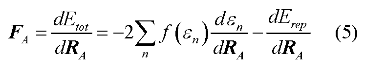
- the force acting on the atom can be calculated by differentiating E tot which is the energy of the whole system with respect to the position RA of the atom.
- a stable atomic arrangement can be calculated by moving the atom so that the force acting on the atom becomes 0 (in the actual simulation, the value input as a parameter or less) from the force acting on the atom thus calculated. it can. This is called structure optimization calculation.
- molecular dynamics calculation can be performed by moving atoms according to the equation of motion from the obtained force.
- the calculation method for obtaining the eigenvalue and wave function of electrons described above has a problem that it takes too much time to calculate a large system because the calculation amount is proportional to the cube of the number of atoms. This may not be suitable for simulation while comparing with experimental data, which requires a reduction in calculation time. Therefore, development of an order N method (O (N) method, where N is the number of atoms to be simulated) in which the amount of calculation is proportional to the number of atoms is in progress as a method for obtaining only the necessary physical quantities in a short time.
- O (N) method where N is the number of atoms to be simulated
- ⁇ i ⁇ represents a localized base
- i represents an atomic site
- ⁇ represents an atomic orbital of a certain atomic site
- C n i ⁇ is a coefficient of ⁇ i ⁇ .
- H j ⁇ , i ⁇ and S j ⁇ , i ⁇ in the equation (8) are defined as follows.
- the density operator can be written as:
- ⁇ i ⁇ , i ⁇ can be expressed as follows.
- the first term on the right side of the equation (4) representing the electron energy can be represented using the matrix elements of the density matrix by substituting the equation (7) and using the equation (12).
- the component related to the electron energy can be expressed as follows.
- ⁇ i ⁇ and i ⁇ represent matrix elements of the energy density matrix.
- ⁇ and ⁇ are quantities that do not depend on the number of atoms.
- localization of the density operator and the energy density operator i.e. the matrix element [rho i.alpha of the density matrix containing a localized basis phi i.alpha and phi Jbeta apart over a certain distance ", Jbeta and ⁇ i ⁇ , j ⁇ is 0 and Because of the physical property that it can be considered, the number of sums of j is constant regardless of the number of atoms. Therefore, the amount of calculation for obtaining energy and force is O (N).
- Structuring optimization and molecular dynamics calculation can be performed using the energy and force thus obtained.
- Divide-and-conquer method divides the entire system into a plurality of regions, obtains the density matrix of the divided region, obtains the physical quantity of the divided region using the density matrix of the divided region, and finally calculates the physical quantity obtained in each region. It is a method that integrates and determines the physical quantity of the entire system. When obtaining the density matrix of the divided area, not only atoms in the divided area but also atoms in an area adjacent to the divided area (referred to as a buffer area) are used.
- FIG. 1 is a diagram schematically showing area division. Circles represent atoms.
- the outer rectangular frame represents the entire system, and the normal dotted line represents the boundary of the divided area.
- the area B surrounded by a thick dotted line other than the area A is a buffer area.
- the physical quantity is calculated as follows.
- the matrix elements ⁇ i ⁇ , j ⁇ of the density matrix are written as follows.
- I is the index of the divided area.
- P (I) ij is defined as follows.
- the regions A and B in FIG. 1 are extracted, and the matrix components are obtained as shown in Equation (9) using the local basis included in the regions.
- the specific formula is as follows.
- the density matrix components of the divided regions are expressed as follows for any Fermi energy.
- the Fermi energy appearing in the Fermi distribution function is obtained.
- the Fermi energy can be obtained from the following condition that “the number N of electrons in the entire system is constant”.
- the Fermi distribution function f ( ⁇ n (I) ) is expressed as follows.
- ⁇ F Fermi energy
- Equation (13) Using the Fermi energy determined by Equation (21) and Equation (22), Equation (13) can be expressed as follows.
- equation (14) is modified as follows.
- ⁇ (I) i ⁇ , j ⁇ is as follows.
- (1) matrix elements in the eigenvalue problem are calculated using localized bases included in the divided areas, and (2) a density matrix for an arbitrary Fermi energy is obtained by solving the eigenvalue problem in each area, (3) The Fermi energy is determined from the condition that the total number of electrons is constant, (4) the physical quantity is calculated from the density matrix of each region, and (5) the physical quantity of the entire system is calculated by taking the sum.
- the size of the buffer area must be set so that the physical quantity to be obtained can be obtained with sufficient accuracy by the calculation system. Normally, the size of the buffer area is determined manually. In addition, a specific physical quantity in the entire system is calculated to determine whether the size of the buffer area is sufficient. A specific physical quantity is a force applied to energy or atoms. Therefore, a specific physical quantity is obtained each time while changing the size of the buffer area, and the size of the buffer area when the specific physical quantity is obtained with sufficient accuracy is adopted.
- the physical quantities of the entire system are calculated as described above, but the size of the buffer area is determined. There is a problem that it takes time to calculate a specific physical quantity only for the purpose. Also, if the size of the buffer area is determined by manually adjusting it, the size of the buffer area cannot be determined efficiently.
- an object of the present technology is to provide a technology for efficiently calculating a buffer area as one aspect.
- This buffer area determination method is a buffer area determination method for determining the number of atomic layers of a buffer area to be set in each of a plurality of areas obtained by dividing a range in which a physical quantity is to be calculated. For each of the regions, the first density matrix in the case where the number of atomic layers in the buffer region is the first number and the second density in the case where the number of atomic layers in the buffer region is a second number different from the first number.
- FIG. 1 is a diagram for explaining a buffer area.
- FIG. 2 is a functional block diagram of the information processing apparatus according to the present embodiment.
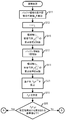
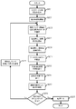
- FIG. 3 is a diagram showing a main processing flow in the present embodiment.
- FIG. 4 is a diagram illustrating a processing flow of search processing.
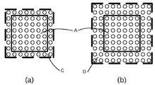
- FIG. 5 is a diagram for explaining the search process.
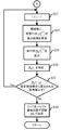
- FIG. 6 is a diagram illustrating a processing flow of search processing.
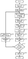
- FIG. 7 is a diagram illustrating a processing flow of search processing.
- FIG. 8 is a diagram illustrating a process flow of the structure optimization process.
- FIG. 9 is a diagram showing a processing flow of molecular dynamics calculation.
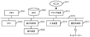
- FIG. 10 is a functional block diagram of a computer.
- FIG. 2 shows a functional block diagram of the information processing apparatus 100 according to an embodiment of the present technology.
- the information processing apparatus 100 includes an input unit 101, a first data storage unit 102, a buffer area determination unit 103, a second data storage unit 104, a physical quantity calculation unit 105, a calculation result storage unit 106, and an output unit. 107.
- the first data storage unit 102 stores an input file 1021 used for processing described below.
- the buffer area determination unit 103 includes a search processing unit 1031 and a density matrix calculation unit 1033, and performs processing using data included in the input file 1021.
- the second data storage unit 104 stores the processing result of the buffer area determination unit 103.
- the physical quantity calculation unit 105 includes a molecular dynamics calculation unit 1051 and a structure optimization unit 1053, and performs processing using data stored in the first data storage unit 102 and the second data storage unit 104.
- the processing result is stored in the calculation result storage unit 106.
- the output unit 107 connects the data stored in the calculation result storage unit 106 according to the data stored in the first data storage unit 102 to an output device (for example, a display device, a printing device, or in some cases connected to a network). To other computers).
- the input unit 101 receives an input from a user and stores the input file 1021 in the first data storage unit 102.
- the input file 1021 stored in another computer connected to the network is stored in the first data storage unit 102 in accordance with an instruction from the user.
- the following data is stored in the input file 1021.
- Calculation conditions (2) Initial atom arrangement (3) Cell information (lattice constant a and unit cell vector) (4) Material band gap E gap (5) Number of divisions in the x, y, and z directions of the region (6) Selection of calculation accuracy judgment condition (energy or force) (7) Energy calculation accuracy ⁇ E input or force calculation accuracy ⁇ F input
- the calculation conditions include the following data. -Initial temperature, final temperature, initial pressure, and final pressure of the system to be calculated (parameters used for temperature control and pressure control (when performing molecular dynamics calculation)) ⁇ Number of atoms ⁇ Number of atomic species ⁇ Maximum number of MD (Molecular Dynamics) steps (at the time of molecular dynamics calculation), or maximum number of structure optimization (at the time of structure optimization) ⁇ Details of output data
- the buffer area determination unit 103 reads the input file from the first data storage unit 102 (step S1). Then, the buffer region determining unit 103 performs region division processing on the entire region specified by the initial atom arrangement according to the number of divisions in the x and z directions of the region (step S3). In this area division processing, each of x, y, and z is divided at equal intervals using a unit lattice vector. Since this processing itself is well known, detailed description thereof is omitted.
- the search processing unit 1031 and the density matrix calculation unit 1033 perform a search process for the number of atomic layers in the buffer area (step S5). This search process will be described with reference to FIGS.
- the search processing unit 1031 calculates an initial value i 0 of the number of atomic layers in the buffer area, and stores it in a storage device such as a main memory (step S11).
- the initial value i 0 is calculated based on the following formula.
- (A) is an expression when the bonding between atoms is strong (for example, a semiconductor), and the coefficient C TB is a value of about 1, for example.
- (B) is an expression when the bond between atoms is weak (for example, metal), and the coefficient CWB is a value of about 1, for example.
- the lattice constant a a value included in the input file 1021 is used. The value included in the input file 1021 is also used for the band gap E gap . Then, ⁇ (
- the calculation process of the density matrix ⁇ i is performed according to the equations (19) to (24). That is, processing for solving the eigenvalue problem is performed. Data in the middle of solving the eigenvalue problem is also stored in the second data storage unit 104, for example. Hamiltonian H (I) and overlap integral matrix S (I) are also calculated when solving these equations, and at least some of the matrix elements are used again later, and are stored in second data storage section 104. Further, Fermi energy ⁇ F is also calculated. The arithmetic processing of this step is well known and will not be described further.
- the density matrix ⁇ i + 1 (I) is stored in, for example, the second data storage unit 104 (step S19).
- an insufficient matrix element may be calculated.
- the Fermi energy is calculated again.
- steps S23 and S25 will be described separately for (A) when energy ⁇ E input is designated as calculation accuracy and (B) when force ⁇ F input is designated as calculation accuracy.
- N (I) element is the larger value of the number of non-zero components of the difference matrix ⁇ (I) and the number of non-zero components of the Hamiltonian H (I) .
- N divide is the number of areas.
- i0 ⁇ 0 and j0 ⁇ 0 are the column element number and row element number of the matrix element that gives the maximum norm of the matrix product of ⁇ (I) and H (I) .
- I 0 is the index value (that is, identifier) of the area that gives the maximum value in the fourth line of equation (29).
- steps S23 and S25 For each region I, specify the column index value i0 ⁇ 0 and the row index value j0 ⁇ 0 of the matrix element that gives the maximum norm in the matrix product of the difference matrix ⁇ (I) and the Hamiltonian H (I) .
- the larger value N (I) element of the number of non-zero components of the difference matrix ⁇ (I) and the number of non-zero components of the Hamiltonian H (I) is specified.
- ⁇ (I) i0 ⁇ 0, j0 ⁇ 0 can be specified in step S23.
- equation (31) If (2) and (3) are performed, the right side (ie, the reference value) of equation (31) can be calculated, and therefore it can be determined in step S23 whether the condition of equation (31) is satisfied.
- N (I) element is the larger value of the number of non-zero components of the difference matrix ⁇ (I) and the number of non-zero components of the Hamiltonian H (I) .
- N divide is the number of areas.
- i0 ⁇ 0 and j0 ⁇ 0 are the column element number and row element number of the matrix element that gives the maximum norm of the matrix product of ⁇ (I) and H (I) .
- I 0 is the index value (that is, identifier) of the area that gives the maximum value in the fourth line of equation (29).
- ⁇ max (I) is the “number of electrons in each region / 2” -th eigenvalue among eigenvalues when the eigenvalue problem is solved in each region. Furthermore, ⁇ max (I0) is ⁇ max (I) of the region I 0 .
- steps S23 and S25 For each region I, specify the column index value i0 ⁇ 0 and the row index value j0 ⁇ 0 of the matrix element that gives the maximum norm in the matrix product of the difference matrix ⁇ (I) and the Hamiltonian H (I) .
- the larger value N (I) element of the number of non-zero components of the difference matrix ⁇ (I) and the number of non-zero components of the Hamiltonian H (I) is specified.
- ⁇ (I) i0 ⁇ 0, j0 ⁇ 0 can be specified in step S23.
- each element of the equation (37) can be extracted from the data obtained when solving the eigenvalue problem, so the right side (ie, the reference value) of the equation (37) is It can also be calculated. Therefore, in step S23, it can be determined whether the condition of the expression (37) is satisfied.
- the buffer area C is set for the divided area A first.
- the buffer area D is set by expanding the buffer area by one layer.
- the condition as in the formula (31) or (37) is satisfied by the characteristic matrix element value in the difference matrix between the density matrix in the case of (a) and the density matrix in the case of (b). Judging.
- step S25 If it is determined in step S25 that ⁇ is equal to or smaller than the reference value calculated from the designated physical quantity, the initial value of the number of atomic layers in the buffer area is too large, and the process proceeds from the terminal A to the processing flow in FIG. . On the other hand, if it is determined in step S25 that ⁇ exceeds the reference value calculated from the designated physical quantity, the initial value of the number of atomic layers in the buffer area is too small, and the processing flow from terminal B to FIG. Migrate to
- the search processing unit 1031 decrements the atomic layer number i by 1 (step S27). That is, the number of atomic layers in the buffer region is reduced by one. For example, consider a case where the buffer area is changed from (b) to (a) in FIG.
- This process is almost the same as step S19.
- the buffer area becomes narrow already calculated matrix elements can be used for the Hamiltonian H (I) and the overlap integral matrix S (I) . That is, data stored in the second data storage unit 104 is used. The Fermi energy is calculated again.
- ⁇ i (I) ⁇ i ⁇ , j ⁇ (I)
- the same calculation as in step S21 is performed.
- step S37: Yes route If ⁇ ⁇ is equal to or smaller than the reference value (step S37: Yes route), the buffer area is still too wide, and the process returns to step S27. On the other hand, if ⁇ ⁇ exceeds the reference value (step S37: Yes route), the search processing unit 1031 determines that (i + 1) The number of layers is determined and stored in the second data storage unit 104 (step S39). Then, returning to the original process, the process of the buffer area determination unit 103 is terminated.
- the characteristic matrix element value in the matrix of the difference between the density matrix before and after the density matrix before changing the number of atomic layers in the buffer region is calculated from the physical quantity specified as the calculation accuracy. It is possible to specify the minimum number of atomic layers satisfying the condition of not more than the value.
- ⁇ i (I) ⁇ i ⁇ , j ⁇ (I)
- step S45 the same calculation as in step S21 is performed.
- step S49: No route If ⁇ + exceeds the reference value (step S49: No route), the buffer area is still small, and the process returns to step S41. On the other hand, when ⁇ + becomes equal to or smaller than the reference value (step S49: Yes route), the search processing unit 1031 determines i as the number of atomic layers in the buffer region and stores it in the second data storage unit 104. (Step S51). Then, returning to the original process, the process of the buffer area determination unit 103 is terminated.
- the characteristic matrix element value in the matrix of the difference between the density matrix before and after the density matrix before changing the number of atomic layers in the buffer region is calculated from the physical quantity specified as the calculation accuracy. It is possible to specify the minimum number of atomic layers satisfying the condition of not more than the value.
- the appropriate number of atomic layers in the buffer area can be calculated. That is, the narrowest buffer area is obtained while maintaining the calculation accuracy of the physical quantity to be calculated. If the buffer area is the narrowest, the calculation amount can be reduced while maintaining the calculation accuracy. Since the physical quantity is not calculated from the density matrix, the calculation amount can be reduced by that amount even if the above-described repetitive processing is performed. Moreover, since the calculation can be performed automatically, the number of atomic layers in the buffer area can be obtained efficiently without depending on the user's skill.
- the number of atomic layers is changed one by one.
- the number of atomic layers is not necessarily limited to 1, and may be changed by other values. Instead of simply increasing or decreasing, convergence may be performed while increasing or decreasing.
- processing by the physical quantity calculation unit 105 is performed using the buffer area thus obtained. Since the processing of the physical quantity calculation unit 105 is the same as the conventional one, it will be briefly described.
- the structure optimization unit 1053 reads the input file 1021 from the first data storage unit 102 and also reads the number of atomic layers in the buffer area stored in the second data storage unit 104 (step S101).
- the structure optimization unit 1053 performs region division processing on the entire region specified by the initial atomic arrangement according to the number of divisions in the x and z directions of the region (step S103).
- this area division processing each of x, y, and z is divided at equal intervals using a unit lattice vector. Since this processing itself is well known, detailed description thereof is omitted.
- the structure optimization unit 1053 may be a processing unit that manages a plurality of processors and the like.
- the atomic data in each fixed buffer area is exchanged by a plurality of processors or the like (step S105).
- the plurality of processors and the like perform processing for searching for neighboring atoms for each region (step S107), and perform processing for solving the eigenvalue problem for each region (step S109). Calculations for the equations (19) to (21) are performed for the assigned area in each processor.
- the structure optimization unit 1053 and the like calculate Fermi energy using the solution of the eigenvalue problem (step S111). Based on the equations (22) and (23), the Fermi energy ⁇ F is calculated by the iterative method using the solution of the eigenvalue problem.
- the structure optimization unit 1053 and the like calculate the density matrix of each region (step S113).
- a density matrix is calculated according to equation (24).
- the structure optimization unit 1053 calculates the physical quantity of the entire system using the density matrix of each region (step S115).
- the electron energy is calculated by the equation (25), and the force applied to the atoms is calculated by the equation (5).
- the structure optimization unit 1053 and the like determine whether or not the force applied to the atoms is larger than the set value (step S117). That is, it is determined whether atoms are stably arranged. It should be noted that there are cases where the atoms are not stably arranged no matter how many times steps S105 to S115 are repeated. In this case, the number of repetitions exceeds the number set in the input file 1021. Also judge.
- the structure optimization unit 1053 or the like When the force applied to the atoms is larger than the set value, the structure optimization unit 1053 or the like performs structure optimization that moves the current atomic position according to the force calculated in step S115, and performs structure optimization.
- the unit 1053 stores data on the current atomic arrangement in the calculation result storage unit 106 (step S119). As a result of this structure optimization process, there are atoms that move across the region, so the atoms moved across the region are exchanged between the plurality of processors (step S121). Then, the process returns to step S105.
- the output unit 107 is stored in the calculation result storage unit 106 according to the settings included in the input file 1021. Data about the latest atomic arrangement is output to an output device or the like (step S123).
- the structure optimization process can be performed using the data on the number of atomic layers in the buffer area.
- the molecular dynamics calculation unit 1051 reads the input file 1021 from the first data storage unit 102 and also reads the number of atomic layers in the buffer area stored in the second data storage unit 104 (step S201).
- the molecular dynamics calculation unit 1051 performs region division processing on the entire region specified by the initial atomic arrangement according to the number of divisions in the x, y, and z directions of the region (step S203).
- this area division processing each of x, y, and z is divided at equal intervals using a unit lattice vector. Since this processing itself is well known, detailed description thereof is omitted.
- the molecular dynamics calculation unit 1051 may be a processing unit that manages a plurality of processors and the like.
- the atomic data in each fixed buffer area is exchanged by a plurality of processors or the like (step S205).
- the plurality of processors and the like perform processing for searching for neighboring atoms for each region (step S207), and perform processing for solving the eigenvalue problem for each region (step S209). Calculations for the equations (19) to (21) are performed for the assigned area in each processor.
- the molecular dynamics calculation unit 1051 and the like calculate Fermi energy using the solution of the eigenvalue problem (step S211). Based on the equations (22) and (23), the Fermi energy ⁇ F is calculated by the iterative method using the solution of the eigenvalue problem.
- the molecular dynamics calculation unit 1051 and the like calculate the density matrix of each region (step S213).
- a density matrix is calculated according to equation (24).
- the molecular dynamics calculation unit 1051 calculates the physical quantity of the entire system using the density matrix of each region (step S215).
- the electron energy is calculated by the equation (25), and the force applied to the atoms is calculated by the equation (5).
- the molecular dynamics calculation unit 1051 and the like move the atom by the equation of motion from the force applied to the atom calculated in step S215 and the unit time step, and the coordinate value of the atom after the movement is stored in the second data storage unit 104. (Step S217).
- the molecular dynamics calculation unit 1051 or the like determines whether or not the time has exceeded the maximum time step set in the input file 1021 (step S219).
- the maximum time step or more has not elapsed, as a result of step S217, there are atoms that move across the region, so the atoms moved across the region are exchanged between the plurality of processors (step S221). .
- the process returns to step S205.
- the output unit 107 outputs the coordinate data of the atom at each time step stored in the calculation result storage unit 106 according to the setting included in the input file 1021.
- the data is output to a device or the like (step S223).
- molecular dynamics calculation can be performed using data on the number of atomic layers in the buffer region.
- the development efficiency will be improved by comparing the experimental results with the simulation results in the development of new materials and devices. Specifically, when obtaining a guideline for determining the temperature and pressure for obtaining the target material and the composition ratio of the material from the simulation result, the development speed can be improved. This leads to a reduction in development time and costs, and a reduction in the environmental burden due to development.
- the present technology is not limited to this.
- the functional block diagram shown in FIG. 2 is an example, and may not necessarily match the actual program module configuration.
- the portions to be executed for each area may be shared by a plurality of processors and computers as described above.
- the buffer area determination method described above can be applied to any method as long as it is a divide-and-conquer method using quantum theory. For example, it can be applied to first-principles calculations and tight-binding calculations.
- the information processing apparatus 100 described above is a computer apparatus, and as shown in FIG. 10, a memory 2501, a CPU 2503, a hard disk drive (HDD) 2505, and a display control unit 2507 connected to the display apparatus 2509.
- a drive device 2513 for the removable disk 2511, an input device 2515, and a communication control unit 2517 for connecting to a network are connected by a bus 2519.
- An operating system (OS: Operating System) and an application program for performing the processing in this embodiment are stored in the HDD 2505, and are read from the HDD 2505 to the memory 2501 when executed by the CPU 2503.
- the CPU 2503 controls the display control unit 2507, the communication control unit 2517, and the drive device 2513 according to the processing content of the application program, and performs a predetermined operation.
- data in the middle of processing is mainly stored in the memory 2501, but may be stored in the HDD 2505.
- an application program for performing the above-described processing is stored in a computer-readable removable disk 2511 and distributed, and installed from the drive device 2513 to the HDD 2505.
- the HDD 2505 may be installed via a network such as the Internet and the communication control unit 2517.
- Such a computer apparatus realizes various functions as described above by organically cooperating hardware such as the CPU 2503 and the memory 2501 described above with programs such as the OS and application programs. .
- This buffer area determination method is a buffer area determination method for determining the number of atomic layers of a buffer area to be set in each of a plurality of areas obtained by dividing a range in which a physical quantity is to be calculated. For each of the regions, the first density matrix in the case where the number of atomic layers in the buffer region is the first number and the second density in the case where the number of atomic layers in the buffer region is a second number different from the first number.
- the search step described above includes (B1) an index of a column of matrix elements that gives a maximum norm in the matrix product of the difference matrix ⁇ (I) and the Hamiltonian H (I) for each of the plurality of regions I. Identifying the value i 0 ⁇ 0 and the row index value j 0 ⁇ 0 , and (B2) for each of the plurality of regions I, the number of non-zero components of the difference matrix ⁇ (I) and the Hamiltonian H (I) identifying the value N (I) element of the larger of the number of non-zero components, (B3) above difference matrix [Delta] [rho] (I) in i 0 alpha 0 column j 0 beta 0 row component value [Delta] [rho] ( I) i0 ⁇ 0, and j0 ⁇ 0, i 0 ⁇ 0 row in Hamiltonian H (I) j 0 ⁇ 0 column component value H (I) j0 ⁇ 0, and I
- the search step described above includes (B5) an index of a column of matrix elements that gives a maximum norm in the matrix product of the difference matrix ⁇ (I) and the Hamiltonian H (I) for each of the plurality of regions I. Identifying the value i 0 ⁇ 0 and the row index value j 0 ⁇ 0 , and (B6) for each of the plurality of regions I, the number of non-zero components of the difference matrix ⁇ (I) and the Hamiltonian H (I ) Specifying the larger value N (I) element of the number of non-zero components in () , and (B7) i 0 ⁇ 0 column j 0 ⁇ 0 row component value ⁇ in the difference matrix ⁇ (I) (I) i0 ⁇ 0, and j0 ⁇ 0, i 0 ⁇ 0 row in Hamiltonian H (I) j 0 ⁇ 0, and I0arufa0, the value N (I)
- a value of a predetermined feature matrix element in a matrix of a difference between the first density matrix for the initial value of the first number and the second density matrix for a value obtained by adding 1 to the initial value of the first number may be increased in the search step, and if it exceeds the reference value, the first number may be decreased in the search step. In this way, the number of atomic layers in the buffer region can be identified efficiently.
- a program for causing a computer to carry out the processing described above such as a flexible disk, an optical disk such as a CD-ROM, a magneto-optical disk, a semiconductor memory (for example, ROM). Or a computer-readable storage medium such as a hard disk or a storage device. Note that data being processed is temporarily stored in a storage device such as a RAM.
Landscapes
- Engineering & Computer Science (AREA)
- Physics & Mathematics (AREA)
- Theoretical Computer Science (AREA)
- General Physics & Mathematics (AREA)
- Evolutionary Computation (AREA)
- General Engineering & Computer Science (AREA)
- Artificial Intelligence (AREA)
- Computational Linguistics (AREA)
- Health & Medical Sciences (AREA)
- Life Sciences & Earth Sciences (AREA)
- Computer Hardware Design (AREA)
- Biomedical Technology (AREA)
- Biophysics (AREA)
- Geometry (AREA)
- Data Mining & Analysis (AREA)
- General Health & Medical Sciences (AREA)
- Molecular Biology (AREA)
- Computing Systems (AREA)
- Mathematical Physics (AREA)
- Software Systems (AREA)
- Management, Administration, Business Operations System, And Electronic Commerce (AREA)
Abstract
効率的にバッファ領域を算出する。本方法は、物理量を計算すべき範囲を分割することによって得られる複数の領域に各々設定すべきバッファ領域の原子層数を決定するバッファ領域決定方法であって、複数の領域の各々について、バッファ領域の原子層数が第1の数である場合における第1の密度行列と、バッファ領域の原子層数が第1の数とは異なる第2の数である場合における第2の密度行列との差の行列を算出し、データ格納部に格納する差行列算出ステップと、第1の数を変化させつつ差行列算出ステップを繰り返し実行させることにより、データ格納部に格納されている上記差の行列における所定の特徴行列要素の値が、指定された物理量から算出される基準値以下である最小の原子層数を探索する探索ステップとを含む。
Description
本技術は、量子論に基づく原子構造又は電子状態の計算技術に関する。
現在、材料学や化学から薬学や生体分野などの新規物質開発において、多くのシミュレーションが行われている。その中で、量子論に基づくシミュレーションを用いる傾向が年々高まっている。これは、すべての物は原子からできているため、開発する物質の性質を予測するためには、原子スケールでの物理現象を理解することが好ましいためである。このような開発では、実験データと比較しながらシミュレーションを行うことになる。そのためには、効率的にシミュレーションを行うためのアプリケーションが好ましい。
まず、量子論に基づいた系のエネルギー又は力の計算方法について説明する。量子論に基づいて物質の原子構造又は電子状態などのシミュレーションを行うためには、ミクロなスケールでの支配方程式であるシュレディンガー方程式を解くことになる。

ここで、Hは系のハミルトニアン、Ψ(r)が電子の波動関数、εが固有値である。
現実の物質には多くの電子が存在している。多くの電子が含まれている系(多電子系と呼ぶ)を計算する1つの手法として、一電子近似がある。一電子近似とは、多電子系をある有効ポテンシャル中における相互作用のない電子の集まりとみなして、電子をエネルギーの低い一電子状態から順番に占有させることによって、多電子系の状態を表す近似方法である。一電子近似を用いると、電子状態は一体のシュレディンガー方程式によって表すことができる。


ここで、Ψeff(r)は有効ポテンシャル、mは電子の質量、 εnはエネルギーが低い順番に並べたときのn番目の状態の電子の固有値、Φn(r)はエネルギーが低い順番に並べたときのn番目の状態の電子の波動関数である。このように、一電子近似を用いることによって、電子状態を計算できる。
一電子近似を用いると全系のエネルギーは、以下のように表される。

ここで、第一項目は電子エネルギー、第二項目Erepは原子核と原子核の相互作用エネルギーと第一項目の電子エネルギーを補正する項である。また、f(εn) はフェルミ分布関数を表す。
また、原子に働く力は、全系のエネルギーであるEtotを原子の位置RAで微分して計算することができる。
このように算出された原子に働く力から、原子に働く力が0(実際のシミュレーションでは、パラメータとして入力した値以下)になるように原子を動かすことによって、安定な原子配置を計算することができる。これを構造最適化計算と呼ぶ。
また、求めた力から運動方程式に従って原子を動かすことによって、分子動力学計算を行うことができる。
上で述べた電子の固有値と波動関数を求める計算方法は、計算量が原子数の三乗に比例するため、大きな系の計算には時間がかかりすぎるという問題がある。これは、計算時間の短縮が求められている、実験データと比較しながらのシミュレーションには向かない場合がある。そのため、必要な物理量だけを短時間で求める方法として、計算量が原子数に比例するオーダーN法(O(N)法、Nはシミュレーションの対象の原子の数)の開発が進められている。
量子論を用いて原子構造又は電子状態を求めるO(N)法では、一電子の固有値と波動関数を求めずに、必要な物理量だけを求める。全系のエネルギーや原子にかかる力をO(N)法を用いて求めるときには、密度行列を導入して計算を行う。ここでは、密度行列を用いたO(N)法の理論を説明する。
電子の波動関数Φnを局在基底で展開すると以下のように表される。

ここで、φiαは局在基底、iは原子のサイト、αはある原子サイトの原子軌道を表す。また、cn
iαはφiαの係数である。(6)式を、ディラックが発明したブラ-ケットの記法を用いると以下のように表すことができる。

このように波動関数をある局在基底で展開すると(2)式のシュレディンガー方程式(微分方程式)を解く問題は、局在基底の係数cn
iαを求める問題(固有値問題)に置き換えることができる。具体的には、(2)式の両辺に左からφ*
jβを掛け、(6)式を代入した後に全空間で積分する。そうすると、以下のような式が得られる。
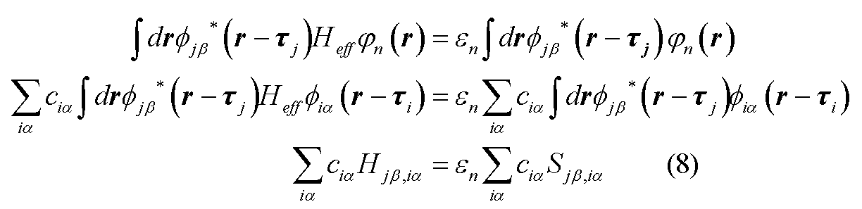
ここで、(8)式のHjβ,iα及びSjβ,iαを以下のように定義する。

(9)式の右辺はブラ-ケットの記法を用いて表したものである。
ここで、密度演算子ρ^(”^”はρの上に載せられているが、ここではこのように記するものとする。)を導入する。密度演算子は以下のように書き表すことができる。

(10)式に(7)式を代入すると、以下の式が得られる。

ここで、ρiα,iβは以下のように表すことができる。

そこで、電子エネルギーを表す(4)式の右辺第一項は、(7)式を代入して(12)式を用いることにより、密度行列の行列要素を用いて表すことができる。

また、(5)式で表した原子にかかる力の項の中で、電子エネルギーに関する成分は以下のように表すことができる。


(13)式と(14)式の4つの和のインデックスのうち、α及びβは原子数に依存しない量である。また、密度演算子とエネルギー密度演算子の局在性、すなわち「ある距離以上に離れた局在基底φiαとφjβを含む密度行列の行列要素ρiα,jβとωiα,jβは0とみなせる」という物理的性質より、jの和の数は原子数によらず一定となる。従って、エネルギーや力を求めるための計算量はO(N)となる。
このようして求めたエネルギーや力を用いて、構造最適化や分子動力学計算を行うことができる。
エネルギーや原子にかかる力を正しく求めるには、「波動関数を求めずに、近傍に存在する2つの局在基底φiαとφjβを含む密度行列の行列要素ρiα,jβをいかに正しく、且つ計算量がO(N)となるように求めるか」が問題となる。その方法として、多くの手法がこれまでに提案されているが、ここでは、分割統治法(Divide-and-Conquer法)に注目することにする。
分割統治法は、全系を複数の領域に分割し、分割した領域の密度行列を求め、分割した領域の密度行列を用いて分割した領域の物理量を求め、最後に各領域で求めた物理量を統合して、系全体の物理量を求める手法である。分割した領域の密度行列を求める際は、分割した領域内の原子だけではなく、分割した領域に隣接する領域(バッファ領域と呼ぶ)の原子も用いる。
図1は、領域分割を模式的に示す図である。丸は原子を表している。外側の矩形枠が全系を表しており、通常の点線が分割した領域の境界を表している。ここで、中央の領域Aに着目すると、領域A以外で太い点線で囲まれた領域Bがバッファ領域である。
具体的には、以下のように物理量を計算する。まず、密度行列の行列要素ρiα,jβを以下のように書き表す。
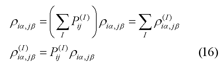
ここで、Iは分割した領域のインデックスである。
ここで、P(I)
ijを以下のように定義する。
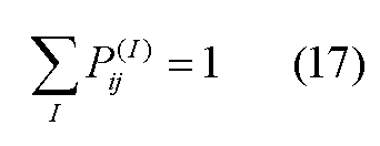

すなわち、局在基底φiαとφjβが両方とも分割した領域(図1の中央の領域)にある場合は、係数「1」を掛け、片方のみ分割した領域にある場合は、0.5を掛け、両方とも分割した領域にない場合は、密度行列を0とする。
そして、分割した領域の密度行列の成分を求めるために、図1の領域A及びBを抜き出し、その領域に含まれる局在基底を用いて(9)式のように行列成分を求める。具体的な式は以下のとおりである。

そして、(19)式を用いて各領域の固有値問題を解く。

各領域の固有値問題を解いて求めた波動関数を用いると、分割した領域の密度行列の成分は任意のフェルミエネルギーに対して、以下のように表される。

ここで注意すべき点は、分割した領域に対して固有値問題を解いたので、(21)式の密度行列の要素は近似した物理量という点である。もちろん、バッファ領域として全系を含むようにとれば、密度行列の要素は厳密な物理量となる。
エネルギーなどの物理量を計算するためには、フェルミ分布関数に現れるフェルミエネルギーを求めることになる。フェルミエネルギーは、「全系の電子数Nが一定」という下記の条件から求めることができる。
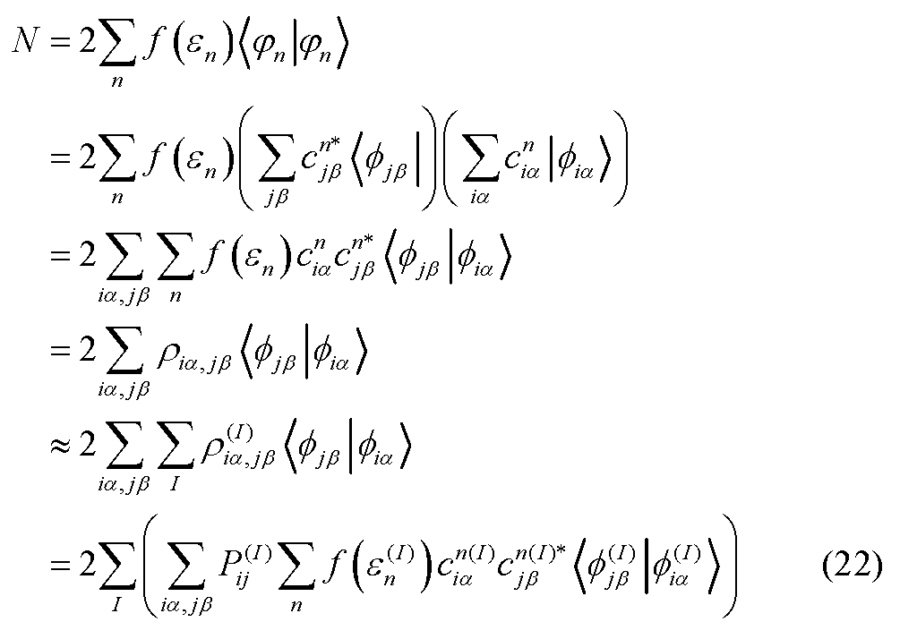
フェルミ分布関数f(εn
(I))は、以下のように表される。

(23)式におけるεFがフェルミエネルギーである。
フェルミエネルギーを決定する際、全系の電子数を求める必要があるので、各領域の電子数のデータを通信する必要がある。
(21)式と(22)式で決定したフェルミエネルギーを用いると、(13)式は以下のように表すことができる。

また、(14)式は、以下のように変形される。
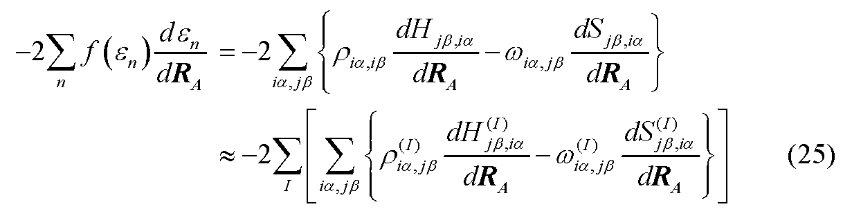
ここで、ω(I)
iα,jβは、以下のとおりである。

以上のように、(1)分割した領域内に含まれる局在基底を用いて固有値問題における行列要素を計算し、(2)各領域において固有値問題を解き任意のフェルミエネルギーに対する密度行列を求め、(3)全電子数は一定という条件からフェルミエネルギーを決定し、(4)各領域の密度行列から物理量を計算し、(5)その和を取ることによって全系の物理量を計算する。
この際留意すべき点は、局在基底φiαとφjβを含む密度行列の行列要素ρiα,jβは、局在基底が近傍にある場合には値を持つため、分割した領域の端(例えば図1における領域Aの外枠内側近傍)の密度行列の行列要素を求めるために、バッファ領域(図1の領域B)を用意することになる点である。
バッファ領域の広さは、計算する系によって、求めるべき物理量が十分な精度で求められるように設定しなければならない。通常は、手動でバッファ領域の広さを決定する。また、バッファ領域の大きさが十分であるかを判断するために、全系における特定の物理量を計算することになる。特定の物理量とは、エネルギーや原子にかかる力である。従って、バッファ領域の大きさを変えながらその都度特定の物理量を求め、特定の物理量が十分な精度で求まった場合におけるバッファ領域の大きさを採用する。
実際には、安定した原子構造を計算したり、原子の移動を計算したりするため、上で述べたように全系の物理量の計算を実施することになるが、バッファ領域の大きさを決定するためだけにも特定の物理量の計算をも行わなければならず、時間が掛ってしまうという問題がある。また、バッファ領域の広さを人手で調節しながら決定するのでは、効率的にバッファ領域の広さを決定できない。
W. Kohn, Int. J. Quart. Chem. 56 (1995) 299
W. Yang, Phys. Rev. Lett. 66 (1991) 1438
従って、本技術の目的は、一側面として、効率的にバッファ領域を算出するための技術を提供することである。
本バッファ領域決定方法は、物理量を計算すべき範囲を分割することによって得られる複数の領域に各々設定すべきバッファ領域の原子層数を決定するバッファ領域決定方法であって、(A)複数の領域の各々について、バッファ領域の原子層数が第1の数である場合における第1の密度行列と、バッファ領域の原子層数が第1の数とは異なる第2の数である場合における第2の密度行列との差の行列を算出し、データ格納部に格納する差行列算出ステップと、(B)第1の数を変化させつつ差行列算出ステップを繰り返し実行させることにより、データ格納部に格納されている上記差の行列における所定の特徴行列要素の値が、指定された物理量から算出される基準値以下である最小の原子層数を探索する探索ステップとを含む。
本技術の一実施の形態に係る情報処理装置100の機能ブロック図を図2に示す。本情報処理装置100は、入力部101と、第1データ格納部102と、バッファ領域決定部103と、第2データ格納部104と、物理量算出部105と、計算結果格納部106と、出力部107とを有する。
第1データ格納部102には、以下で説明する処理に用いる入力ファイル1021が格納される。バッファ領域決定部103は、探索処理部1031と密度行列算出部1033とを有し、入力ファイル1021に含まれるデータを用いて処理等を実施する。第2データ格納部104は、バッファ領域決定部103の処理結果を格納する。物理量算出部105は、分子動力学計算部1051と構造最適化部1053とを有し、第1データ格納部102及び第2データ格納部104に格納されているデータを用いて処理を実施し、処理結果を計算結果格納部106に格納する。出力部107は、第1データ格納部102に格納されているデータに従って、計算結果格納部106に格納されているデータを、出力装置(例えば表示装置、印刷装置、場合によってはネットワークに接続されている他のコンピュータなど)に出力する。
次に、図2に示した情報処理装置100の動作について図3乃至図9を用いて説明する。入力部101は、ユーザからの入力を受け付けて、入力ファイル1021を第1データ格納部102に格納する。場合によっては、ユーザからの指示に応じて、ネットワークに接続されている他のコンピュータに格納されている入力ファイル1021を第1データ格納部102に格納する。
入力ファイル1021には、例えば、以下のようなデータが格納される。
(1)計算条件
(2)初期原子配置
(3)セルの情報(格子定数aと単位格子ベクトル)
(4)物質のバンドギャップEgap
(5)領域のx、y及びz方向の分割数
(6)計算精度の判定条件(エネルギー又は力)の選択
(7)エネルギーの計算精度ΔEinput又は力の計算精度ΔFinput
(1)計算条件
(2)初期原子配置
(3)セルの情報(格子定数aと単位格子ベクトル)
(4)物質のバンドギャップEgap
(5)領域のx、y及びz方向の分割数
(6)計算精度の判定条件(エネルギー又は力)の選択
(7)エネルギーの計算精度ΔEinput又は力の計算精度ΔFinput
また、計算条件には、以下のようなデータを含む。
・計算する系の初期温度、最終温度、初期圧力、最終圧力(温度制御や圧力制御を行うときに用いられるパラメータ(分子動力学計算を行う場合))
・原子数
・原子種の数
・MD(Molecular Dynamics)最大ステップ数(分子動力学計算時)、又は構造最適化の最大回数(構造最適化時)
・出力データの詳細度など
・計算する系の初期温度、最終温度、初期圧力、最終圧力(温度制御や圧力制御を行うときに用いられるパラメータ(分子動力学計算を行う場合))
・原子数
・原子種の数
・MD(Molecular Dynamics)最大ステップ数(分子動力学計算時)、又は構造最適化の最大回数(構造最適化時)
・出力データの詳細度など
そして、バッファ領域決定部103は、第1データ格納部102から入力ファイルを読み出す(ステップS1)。そして、バッファ領域決定部103は、初期原子配置で特定される領域全体を、領域のx、及びz方向の分割数に従って領域分割処理を実施する(ステップS3)。この領域分割処理では、単位格子ベクトルを用いてx、y及びzのそれぞれについて等間隔に分割するが、この処理自体はよく知られたものであるから、詳細な説明については省略する。
そして、探索処理部1031及び密度行列算出部1033は、バッファ領域の原子層数についての探索処理を実施する(ステップS5)。この探索処理については、図4乃至図7を用いて説明する。
まず、探索処理部1031は、バッファ領域の原子層数の初期値i0を算出し、例えばメインメモリなどの記憶装置に格納する(ステップS11)。初期値i0については、以下の式に基づき算出する。

この式において|r-r'|が、求めるべきバッファ領域の原子層数の初期値となる。また、Kは、以下のように算出される。
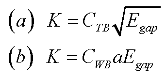
(a)は原子間の結合が強い場合(例えば半導体など)の式であり、係数CTBは、例えば1程度の値である。(b)は原子間の結合が弱い場合(例えば金属)の式であり、係数CWBは、例えば1程度の値である。格子定数aは、入力ファイル1021に含まれている値を用いる。バンドギャップEgapについても、入力ファイル1021に含まれる値を用いる。そして、ρ(|r-r'|)にはほぼ10-5程度として設定し、|r-r'|を算出する。このようにすれば、原子間の相互作用が無視できる程度の値(10-5)になるようなバッファ領域の原子層数|r-r'|が得られるようになる。
そして、探索処理部1031は、iに初期値i0を設定する(ステップS13)。その後、探索処理部1031は、密度行列算出部1033に、密度行列ρi
(I)=ρiα,jβ
(I),beforeの算出処理を領域毎に実施させ、密度行列ρi
(I)を例えば第2データ格納部104に格納させる(ステップS15)。
密度行列ρiの算出処理については、(19)式乃至(24)式に従って行われる。すなわち、固有値問題を解く処理を実施することになる。固有値問題を解く際の途中のデータについても例えば第2データ格納部104に格納しておく。ハミルトニアンH(I)及び重なり積分行列S(I)もこれらの式を解く際に算出され、後に少なくとも一部の行列要素については再度使用されるので、第2データ格納部104に格納される。さらに、フェルミエネルギーεFについても算出される。このステップの演算処理については、よく知られているので、これ以上述べない。
次に、探索処理部1031は、バッファ領域の原子層数iを1層増加させ(ステップS17)、密度行列算出部1033に、密度行列ρi+1
(I)(=ρiα,jβ
(I),after)の算出処理を領域毎に実施させ、密度行列ρi+1
(I)を例えば第2データ格納部104に格納させる(ステップS19)。ハミルトニアンH(I)及び重なり積分行列S(I)については、不足する行列要素を算出すればよい。また、フェルミエネルギーについては再度算出する。
その後、探索処理部1031は、各領域について差行列Δρ(I)=Δρiα,jβ
(I)を算出し、例えば第2データ格納部104に格納する(ステップS21)。具体的には、以下の式にて算出される。
Δρiα,jβ (I)=ρiα,jβ (I),after-ρiα,jβ (I),before
Δρiα,jβ (I)=ρiα,jβ (I),after-ρiα,jβ (I),before
そして、探索処理部1031は、第2データ格納部104に格納されている差行列Δρ(I)=Δρiα,jβ
(I)のうち特徴となる行列要素Δρ=Δρi0α0,j0β0
(I)を特定する(ステップS23)。そして、探索処理部1031は、Δρが、計算精度として指定された物理量から算出される基準値以下であるか判断する(ステップS25)。
ステップS23及びS25の処理について、(A)エネルギーΔEinputが計算精度として指定された場合、(B)力ΔFinputが計算精度として指定された場合に分けて説明する。
(a)エネルギーΔEinputの場合
バッファ領域の原子層を変化させる前と変化させた後の電子系のエネルギーは(24)式から以下のようになる。
バッファ領域の原子層を変化させる前と変化させた後の電子系のエネルギーは(24)式から以下のようになる。
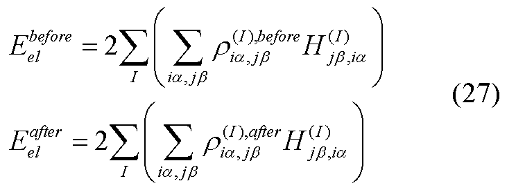
そうすると、バッファ領域の原子層を変化させる前と変化させた後のエネルギーの差は、以下のように表される。

さらに、(28)式の絶対値の上限は、以下のように表される。

ここで、N(I)
elementは、差行列Δρ(I)の非零成分の数とハミルトニアンH(I)の非零成分の数のうち、大きい方の値である。また、Ndivideは領域数である。さらに、i0α0,j0β0は、Δρ(I)とH(I)の行列積の最大ノルムを与える行列要素の列要素番号と行要素番号である。I0は(29)式の4行目において最大値を与える領域のインデックス値(すなわち識別子)である。
(29)式により、入力したエネルギーの精度ΔEinputを満たすためには以下の式を満たせばよい。

そのため、入力したエネルギーの精度ΔEinputを保つ条件は以下のとおりである。

従って、ステップS23及びS25のために以下の処理を実施する。
(1)各領域Iについて、差行列Δρ(I)とハミルトニアンH(I)との行列積において最大ノルムを与える行列要素の列のインデックス値i0α0及び行のインデックス値j0β0を特定する。
(2)各領域Iについて、差行列Δρ(I)の非零成分の数とハミルトニアンH(I)の非零成分の数とのうち大きい方の値N(I) elementを特定する。
(3)差行列Δρ(I)におけるi0α0列j0β0行成分値Δρ(I) i0α0,j0β0と、ハミルトニアンH(I)におけるi0α0行j0β0列成分値H(I) j0β0,i0α0と、N(I) elementとの積が最大となる領域のインデックス値I0を特定する。
(1)各領域Iについて、差行列Δρ(I)とハミルトニアンH(I)との行列積において最大ノルムを与える行列要素の列のインデックス値i0α0及び行のインデックス値j0β0を特定する。
(2)各領域Iについて、差行列Δρ(I)の非零成分の数とハミルトニアンH(I)の非零成分の数とのうち大きい方の値N(I) elementを特定する。
(3)差行列Δρ(I)におけるi0α0列j0β0行成分値Δρ(I) i0α0,j0β0と、ハミルトニアンH(I)におけるi0α0行j0β0列成分値H(I) j0β0,i0α0と、N(I) elementとの積が最大となる領域のインデックス値I0を特定する。
(1)を実施すれば、ステップS23で、Δρ(I)
i0α0,j0β0を特定することができる。
(2)及び(3)を実施すれば、(31)式の右辺(すなわち基準値)を算出することができるので、ステップS23において(31)式の条件を満たすか判断することができる。
(B)力ΔFinputの場合
バッファ領域の原子層を変化させる前と変化させた後の電子系の力は(25)式から以下のように表される。
バッファ領域の原子層を変化させる前と変化させた後の電子系の力は(25)式から以下のように表される。


そうすると、原子層を変化させる前と後との力の差の絶対値は以下のように表される。

この力の差の絶対値の上限は以下のように表される。
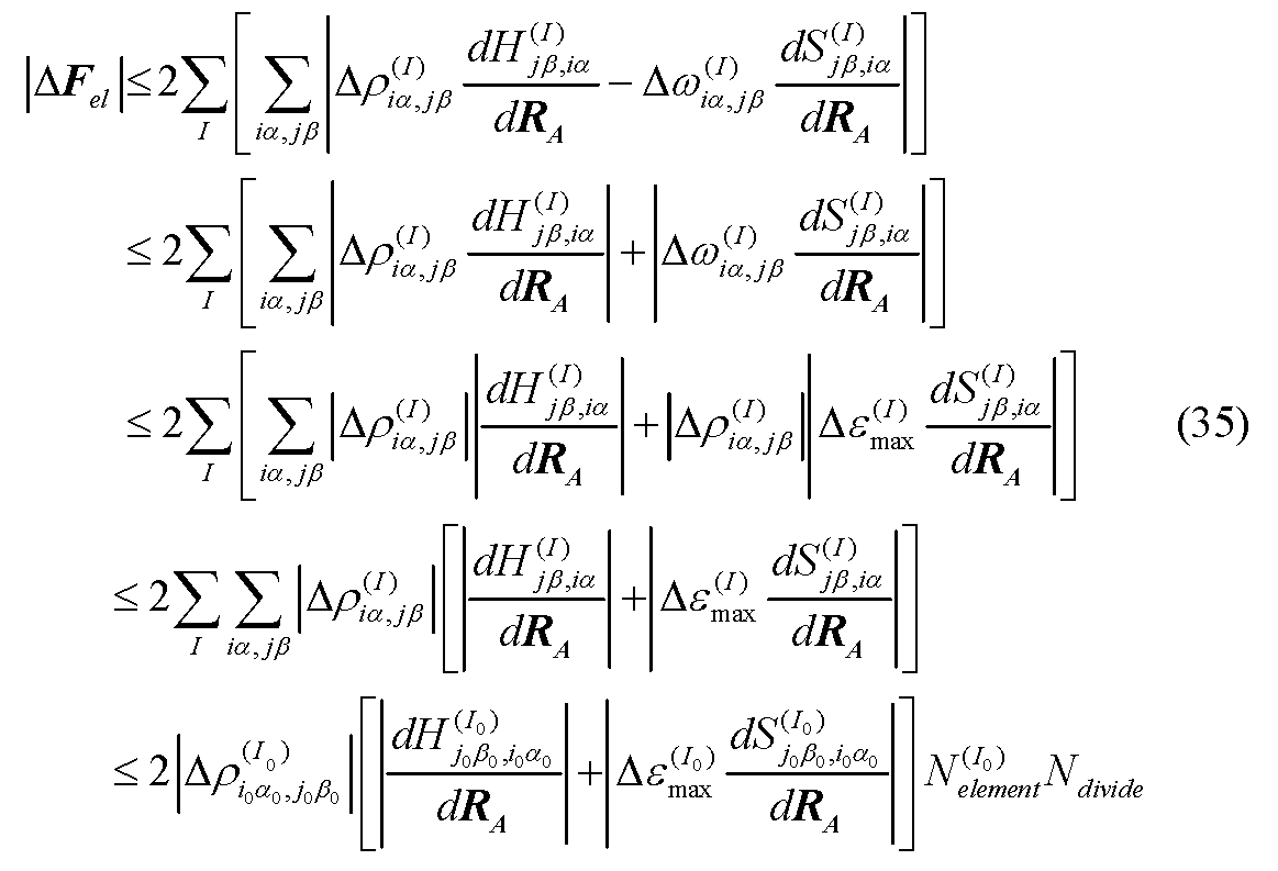
なお、RAは原子の座標値を表す。また、N(I)
elementは、差行列Δρ(I)の非零成分の数とハミルトニアンH(I)の非零成分の数のうち、大きい方の値である。また、Ndivideは領域数である。さらに、i0α0,j0β0は、Δρ(I)とH(I)の行列積の最大ノルムを与える行列要素の列要素番号と行要素番号である。I0は(29)式の4行目において最大値を与える領域のインデックス値(すなわち識別子)である。さらに、εmax
(I)は、各領域で固有値問題を解いたときの固有値のうち「各領域内の電子数/2」番目の固有値である。さらに、εmax
(I0)は、領域I0のεmax
(I)である。
(35)式から、入力された力の精度ΔFinputを満たすためには以下の式を満たせばよい。

そのため、入力した力の精度ΔFinputを保つ条件は以下のとおりである。
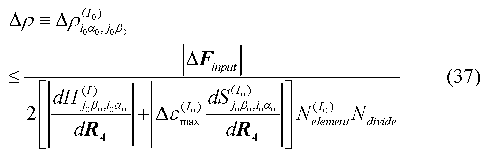
従って、ステップS23及びS25のために以下の処理を実施する。
(1)各領域Iについて、差行列Δρ(I)とハミルトニアンH(I)との行列積において最大ノルムを与える行列要素の列のインデックス値i0α0及び行のインデックス値j0β0を特定する。
(2)各領域Iについて、差行列Δρ(I)の非零成分の数とハミルトニアンH(I)の非零成分の数とのうち大きい方の値N(I) elementを特定する。
(3)差行列Δρ(I)におけるi0α0列j0β0行成分値Δρ(I) i0α0,j0β0と、ハミルトニアンH(I)におけるi0α0行j0β0列成分値H(I) j0β0,i0α0と、N(I) elementとの積が最大となる領域のインデックス値I0を特定する。
(1)各領域Iについて、差行列Δρ(I)とハミルトニアンH(I)との行列積において最大ノルムを与える行列要素の列のインデックス値i0α0及び行のインデックス値j0β0を特定する。
(2)各領域Iについて、差行列Δρ(I)の非零成分の数とハミルトニアンH(I)の非零成分の数とのうち大きい方の値N(I) elementを特定する。
(3)差行列Δρ(I)におけるi0α0列j0β0行成分値Δρ(I) i0α0,j0β0と、ハミルトニアンH(I)におけるi0α0行j0β0列成分値H(I) j0β0,i0α0と、N(I) elementとの積が最大となる領域のインデックス値I0を特定する。
(1)を実施すれば、ステップS23で、Δρ(I)
i0α0,j0β0を特定することができる。
(2)及び(3)を実施すれば、固有値問題を解く際に得られたデータから(37)式の各要素を抽出することができるので、(37)式の右辺(すなわち基準値)を算出することもできる。従って、ステップS23において(37)式の条件を満たすか判断することができる。
ここまでの処理を模式的に示すと図5のようになる。図5の(a)では、分割領域Aに対して、最初にバッファ領域Cを設定している。そして、図5の(b)で示すように、1層だけバッファ領域を拡張してバッファ領域Dを設定する。この際に、(31)式又は(37)式のような条件を、(a)の場合の密度行列と(b)の場合の密度行列の差の行列における特徴的な行列要素値が満たしているか判断している。
ステップS25においてΔρが、指定物理量から算出される基準値以下であると判断されると、バッファ領域の原子層数の初期値は大きすぎたということで端子Aから図6の処理フローに移行する。一方、ステップS25においてΔρが、指定物理量から算出される基準値を超えていると判断されると、バッファ領域の原子層数の初期値は小さすぎたということで端子Bから図7の処理フローに移行する。
図6の処理フローの説明に移行して、探索処理部1031は、原子層数iを1デクリメントする(ステップS27)。すなわち、バッファ領域の原子層数を1削減する。例えば、バッファ領域を図5の(b)から(a)に変化させる場合を考える。
そして、探索処理部1031は、バッファ領域の原子層数を1削減した状態において、密度行列算出部1033に密度行列ρi-1の算出処理を領域毎に実施させ、密度行列ρi-1
(I)(=ρiα,jβ
(I),after)を例えば第2データ格納部104に格納させる(ステップS31)。この処理は、ステップS19とほぼ同様である。但し、バッファ領域が狭くなる場合には、ハミルトニアンH(I)及び重なり積分行列S(I)については、既に計算済みの行列要素を用いることができる。すなわち、第2データ格納部104に格納されているデータを利用する。フェルミエネルギーについては再度算出する。
そして、探索処理部1031は、各領域について差行列Δρ(I)
-(=Δρiα,jβ
(I))を算出し、例えば第2データ格納部104に格納する(ステップS33)。ρi
(I)=ρiα,jβ
(I),beforeとして、ステップS21と同様の演算を実施する。
そして、探索処理部1031は、第2データ格納部104に格納されている差行列Δρ(I)
-(=Δρiα,jβ
(I))のうち特徴となる行列要素Δρ-(=Δρi0α0,j0β0
(I))を特定する(ステップS35)。このステップでもステップS23と同様の演算を実施する。その後、探索処理部1031は、Δρ-が、計算精度として指定された物理量から算出される基準値以下であるか判断する(ステップS37)。このステップにおいても、ステップS25と同様の演算により基準値を算出した上で、Δρ-と比較を行う。
Δρ-が、基準値以下である場合には(ステップS37:Yesルート)、まだバッファ領域が広すぎるので、ステップS27に戻る。一方、Δρ-が、基準値を超えた場合には(ステップS37:Yesルート)、バッファ領域を1原子層狭くしすぎたということで、探索処理部1031は、(i+1)をバッファ領域の原子層数として決定し、第2データ格納部104に格納する(ステップS39)。そして元の処理に戻って、バッファ領域決定部103の処理を終了する。
このようにすれば、バッファ領域の原子層数を変化させる前の密度行列と後の密度行列との差の行列における特徴的な行列要素値が、計算精度として指定された物理量から算出される基準値以下という条件を満たす最小の原子層数を特定することができる。
次に、端子B以降の処理を図7を用いて説明する。図7で説明する処理は、図5の(a)から(b)のようにバッファ領域の広さを広げてゆく処理である。まず、探索処理部1031は、原子層数iを1インクリメントする(ステップS41)。そして、探索処理部1031は、バッファ領域の原子層数を1増加した状態において、密度行列算出部1033に密度行列ρi+1の算出処理を領域毎に実施させ、密度行列ρi+1
(I)(=ρiα,jβ
(I),after)を例えば第2データ格納部104に格納させる(ステップS43)。この処理は、ステップS19とほぼ同様である。但し、バッファ領域が広くなるので、ハミルトニアンH(I)及び重なり積分行列S(I)については、新たに追加された領域に含まれる原子について不足する行列要素を追加で算出し、既に算出されているものについてはそのまま使用する。フェルミエネルギーについては再度算出する。
そして、探索処理部1031は、各領域について差行列Δρ(I)
+(=Δρiα,jβ
(I))を算出し、例えば第2データ格納部104に格納する(ステップS45)。ρi
(I)=ρiα,jβ
(I),beforeとして、ステップS21と同様の演算を実施する。
そして、探索処理部1031は、第2データ格納部104に格納されている差行列Δρ(I)
+(=Δρiα,jβ
(I))のうち特徴となる行列要素Δρ+(=Δρi0α0,j0β0
(I))を特定する(ステップS47)。このステップでもステップS23と同様の演算を実施する。その後、探索処理部1031は、Δρ+が、計算精度として指定された物理量から算出される基準値以下であるか判断する(ステップS49)。このステップにおいても、ステップS25と同様の演算により基準値を算出した上で、Δρ+と比較を行う。
Δρ+が、基準値を超えている場合には(ステップS49:Noルート)、まだバッファ領域が狭いので、ステップS41に戻る。一方、Δρ+が、基準値以下になった場合には(ステップS49:Yesルート)、探索処理部1031は、iをバッファ領域の原子層数として決定し、第2データ格納部104に格納する(ステップS51)。そして元の処理に戻って、バッファ領域決定部103の処理を終了する。
このようにすれば、バッファ領域の原子層数を変化させる前の密度行列と後の密度行列との差の行列における特徴的な行列要素値が、計算精度として指定された物理量から算出される基準値以下という条件を満たす最小の原子層数を特定することができる。
以上のような処理を実施することで、バッファ領域の適切な原子層数を算出することができる。すなわち、これから計算する物理量の計算精度を維持しつつ、最も狭いバッファ領域が得られたことになる。最も狭いバッファ領域であれば、計算精度を維持しつつ計算量を削減できることになる。なお、密度行列から物理量を算出することがないので、上で述べたような繰り返し処理を実施したとしても、その分だけ計算量を削減することができている。また、自動で計算できているため、ユーザのスキルなどに依存せず効率的にバッファ領域の原子層数が得られている。
なお、上ではコンピュータ1台で処理を実施する例を示したが、領域毎に行う演算については複数のプロセッサ(すなわちCPU:Central Processing Unit)又は複数のコンピュータで並列して演算することも可能である。
さらに、上で述べた処理フローでは、原子層数を1つずつ変化させているが、必ずしも1に限定されるものではなく、他の値ずつ変化させるようにしても良い。単純増加又は減少ではなく、増減させながら収束させるようにしても良い。
なお、この後、このようにして得られたバッファ領域を用いて物理量算出部105による処理が行われる。物理量算出部105の処理については、従来と同様であるから、簡単に説明しておく。
まず、構造最適化部1053等による、原子構造の最適化のための処理を、図8を用いて説明する。まず、構造最適化部1053は、第1データ格納部102から入力ファイル1021を読み出すと共に、第2データ格納部104に格納されているバッファ領域の原子層数を読み出す(ステップS101)。
そして、構造最適化部1053は、初期原子配置で特定される領域全体を、領域のx、及びz方向の分割数に従って領域分割処理を実施する(ステップS103)。この領域分割処理では、単位格子ベクトルを用いてx、y及びzのそれぞれについて等間隔に分割するが、この処理自体はよく知られたものであるから、詳細な説明については省略する。
以下の処理については、複数のプロセッサなどで並列実施する場合を想定して説明する。よって、領域分割後の各領域に属する原子のデータを、担当するプロセッサ等に配布する。なお、構造最適化部1053は、複数のプロセッサ等の管理を行う処理部であっても良い。
そして、第2データ格納部104に格納されているバッファ領域の原子層数に従って、各確定バッファ領域内にある原子のデータを、複数のプロセッサ等で交換する(ステップS105)。その後、複数のプロセッサ等は、領域毎に、近傍原子を探索する処理を実施して(ステップS107)、領域毎に固有値問題を解く処理を実施する(ステップS109)。(19)式乃至(21)式についての演算を、各プロセッサで、担当領域について実施する。
さらに、構造最適化部1053等は、固有値問題の解を用いてフェルミエネルギーを算出する(ステップS111)。(22)式及び(23)式に基づき、固有値問題の解を用いて反復法によってフェルミエネルギーεFを算出する。
そして、構造最適化部1053等は、各領域の密度行列を算出する(ステップS113)。(24)式に従って密度行列を算出する。その後、構造最適化部1053は、各領域の密度行列を用いて全系の物理量を算出する(ステップS115)。(25)式によって電子エネルギーが算出され、(5)式によって原子にかかる力が算出される。
そして、構造最適化部1053等は、原子にかかる力が設定した値より大きいか判断する(ステップS117)。すなわち、安定的に原子が配置されているかを判断する。なお、何回ステップS105乃至S115を繰り返し実施しても安定的に原子が配置されていることにならない場合もあるので、その場合には入力ファイル1021に設定されている回数を超えて繰り返しているかをも判断する。
原子にかかる力が設定した値より大きい場合には、構造最適化部1053等は、現在の原子位置を、ステップS115で算出された力に応じて移動させる構造最適化を実施し、構造最適化部1053は、現在の原子配置についてのデータを計算結果格納部106に格納する(ステップS119)。この構造最適化処理の結果、領域をまたいで移動する原子も存在するので、領域をまたいで移動した原子を、複数のプロセッサ間で交換する(ステップS121)。そして、ステップS105に戻る。
一方、原子にかかる力が設定した値以下である場合又は繰り返し回数が設定回数を超えている場合には、出力部107は、入力ファイル1021に含まれる設定に従って、計算結果格納部106に格納されている最新の原子配置についてのデータを出力装置等に出力する(ステップS123)。
このように、バッファ領域の原子層数のデータを用いて構造最適化処理を実施することができる。
また、分子動力学計算部1051等による、分子動力学のための処理を、図9を用いて説明する。まず、分子動力学計算部1051は、第1データ格納部102から入力ファイル1021を読み出すと共に、第2データ格納部104に格納されているバッファ領域の原子層数を読み出す(ステップS201)。
そして、分子動力学計算部1051は、初期原子配置で特定される領域全体を、領域のx、y及びz方向の分割数に従って領域分割処理を実施する(ステップS203)。この領域分割処理では、単位格子ベクトルを用いてx、y及びzのそれぞれについて等間隔に分割するが、この処理自体はよく知られたものであるから、詳細な説明については省略する。
以下の処理については、複数のプロセッサなどで並列実施する場合を想定して説明する。よって、領域分割後の各領域に属する原子のデータを、担当するプロセッサ等に配布する。なお、分子動力学計算部1051は、複数のプロセッサ等の管理を行う処理部であっても良い。
そして、第2データ格納部104に格納されているバッファ領域の原子層数に従って、各確定バッファ領域内にある原子のデータを、複数のプロセッサ等で交換する(ステップS205)。その後、複数のプロセッサ等は、領域毎に、近傍原子を探索する処理を実施して(ステップS207)、領域毎に固有値問題を解く処理を実施する(ステップS209)。(19)式乃至(21)式についての演算を、各プロセッサで、担当領域について実施する。
さらに、分子動力学計算部1051等は、固有値問題の解を用いてフェルミエネルギーを算出する(ステップS211)。(22)式及び(23)式に基づき、固有値問題の解を用いて反復法によってフェルミエネルギーεFを算出する。
そして、分子動力学計算部1051等は、各領域の密度行列を算出する(ステップS213)。(24)式に従って密度行列を算出する。その後、分子動力学計算部1051は、各領域の密度行列を用いて全系の物理量を算出する(ステップS215)。(25)式によって電子エネルギーが算出され、(5)式によって原子にかかる力が算出される。
その後、分子動力学計算部1051等は、ステップS215で算出された原子にかかる力と単位タイムステップとから運動方程式により原子を移動させ、移動後の原子の座標値などを第2データ格納部104に格納する(ステップS217)。
そして、分子動力学計算部1051等は、時間が、入力ファイル1021において設定されている最大タイムステップ以上経過したか判断する(ステップS219)。最大タイムステップ以上経過していない場合には、ステップS217の結果として、領域をまたいで移動する原子も存在するので、領域をまたいで移動した原子を、複数のプロセッサ間で交換する(ステップS221)。そして、ステップS205に戻る。
一方、時間が、設定された最大タイムステップ以上経過した場合、出力部107は、入力ファイル1021に含まれる設定に従って、計算結果格納部106に格納されている各タイムステップにおける原子の座標データを出力装置等に出力する(ステップS223)。
このように、バッファ領域の原子層数のデータを用いて分子動力学の計算を実施することができる。
このような処理を実施することで、新材料・デバイス開発において、実験結果とシミュレーション結果を照らし合わせた開発効率が向上する。具体的には、目的とする材料を得るための温度や圧力、材料の組成比を決定するための指針をシミュレーション結果から得る際、その開発速度を向上させることができる。これは、開発時間と経費の削減、開発による環境負荷の低減につながる。
以上本技術の実施の形態を説明したが、本技術はこれに限定されるものではない。例えば、図2に示した機能ブロック図は一例であって、必ずしも実際のプログラムモジュール構成と一致しない場合がある。処理フローについても、各領域について実施する部分については、上で述べたように複数のプロセッサやコンピュータで分担して実行するようにしても良い。
なお、本技術によれば、上で述べたバッファ領域の決定方法は、量子論を用いた分割統治法であれば、どんな手法にも対応することが出来る。例えば、第一原理計算、タイトバインディング計算に適用することができる。
なお、上で述べた情報処理装置100は、コンピュータ装置であって、図10に示すように、メモリ2501とCPU2503とハードディスク・ドライブ(HDD)2505と表示装置2509に接続される表示制御部2507とリムーバブル・ディスク2511用のドライブ装置2513と入力装置2515とネットワークに接続するための通信制御部2517とがバス2519で接続されている。オペレーティング・システム(OS:Operating System)及び本実施例における処理を実施するためのアプリケーション・プログラムは、HDD2505に格納されており、CPU2503により実行される際にはHDD2505からメモリ2501に読み出される。CPU2503は、アプリケーション・プログラムの処理内容に応じて表示制御部2507、通信制御部2517、ドライブ装置2513を制御して、所定の動作を行わせる。また、処理途中のデータについては、主としてメモリ2501に格納されるが、HDD2505に格納されるようにしてもよい。本技術の実施例では、上で述べた処理を実施するためのアプリケーション・プログラムはコンピュータ読み取り可能なリムーバブル・ディスク2511に格納されて頒布され、ドライブ装置2513からHDD2505にインストールされる。インターネットなどのネットワーク及び通信制御部2517を経由して、HDD2505にインストールされる場合もある。このようなコンピュータ装置は、上で述べたCPU2503、メモリ2501などのハードウエアとOS及びアプリケーション・プログラムなどのプログラムとが有機的に協働することにより、上で述べたような各種機能を実現する。
以上述べた本実施の形態をまとめると、以下のようになる。
本バッファ領域決定方法は、物理量を計算すべき範囲を分割することによって得られる複数の領域に各々設定すべきバッファ領域の原子層数を決定するバッファ領域決定方法であって、(A)複数の領域の各々について、バッファ領域の原子層数が第1の数である場合における第1の密度行列と、バッファ領域の原子層数が第1の数とは異なる第2の数である場合における第2の密度行列との差の行列を算出し、データ格納部に格納する差行列算出ステップと、(B)第1の数を変化させつつ差行列算出ステップを繰り返し実行させることにより、データ格納部に格納されている上記差の行列における所定の特徴行列要素の値が、指定された物理量から算出される基準値以下である最小の原子層数を探索する探索ステップとを含む。
このように密度行列に着目して実際に物理量を計算することなくバッファ領域の原子層数の適切な値を高速に算出することができるようになる。
なお、上で述べた探索ステップが、(B1)複数の領域Iの各々について、上記差の行列Δρ(I)とハミルトニアンH(I)との行列積において最大ノルムを与える行列要素の列のインデックス値i0α0及び行のインデックス値j0β0を特定するステップと、(B2)複数の領域Iの各々について、差の行列Δρ(I)の非零成分の数とハミルトニアンH(I)の非零成分の数とのうち大きい方の値N(I)
elementを特定するステップと、(B3)上記差の行列Δρ(I)におけるi0α0列j0β0行成分値Δρ(I)
i0α0,j0β0と、ハミルトニアンH(I)におけるi0α0行j0β0列成分値H(I)
j0β0,i0α0と、値N(I)
elementとの積が最大となる領域の識別子I0を特定するステップと、(B4)指定された物理量であるエネルギーΔEinputと複数の領域の数Ndivideとから、
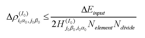
を満たしているか判断するステップとを含むようにしてもよい。エネルギーの計算精度が指定された場合にも対処可能である。
さらに、上で述べた探索ステップが、(B5)複数の領域Iの各々について、上記差の行列Δρ(I)とハミルトニアンH(I)との行列積において最大ノルムを与える行列要素の列のインデックス値i0α0及び行のインデックス値j0β0を特定するステップと、(B6)複数の領域Iの各々について、上記差の行列Δ(I)の非零成分の数とハミルトニアンH(I)の非零成分の数とのうち大きい方の値N(I)
elementを特定するステップと、(B7)上記差の行列Δρ(I)におけるi0α0列j0β0行成分値Δρ(I)
i0α0,j0β0と、ハミルトニアンH(I)におけるi0α0行j0β0列成分値H(I)
j0β0,i0α0と、値N(I)
elementとの積が最大となる領域の識別子I0を特定するステップと、(B8)指定された物理量である力ΔFinputの絶対値と複数の領域の数Ndivideと重なり積分行列S(I)におけるi0α0行j0β0列成分値S(I)
j0β0,i0α0と領域I0における(電子数/2)番目の固有値εmax
Iと原子の座標RAとから、

を満たしているか判断するステップとを含むようにしてもよい。力の計算精度が指定された場合にも対処可能である。
さらに、第1の数の初期値についての第1の密度行列と第1の数の初期値に1を加えた値についての第2の密度行列との差の行列における所定の特徴行列要素の値が、基準値以下であれば探索ステップにおいて第1の数を増加させ、基準値を超える場合には探索ステップにおいて第1の数を減少させるようにしてもよい。このようにすれば、効率的にバッファ領域の原子層数を特定できる。
なお、上で述べたような処理をコンピュータに実施させるためのプログラムを作成することができ、当該プログラムは、例えばフレキシブル・ディスク、CD-ROMなどの光ディスク、光磁気ディスク、半導体メモリ(例えばROM)、ハードディスク等のコンピュータ読み取り可能な記憶媒体又は記憶装置に格納される。なお、処理途中のデータについては、RAM等の記憶装置に一時保管される。
Claims (6)
- 物理量を計算すべき範囲を分割することによって得られる複数の領域に各々設定すべきバッファ領域の原子層数を決定させる処理を、コンピュータに実行させるプログラムであって、
前記複数の領域の各々について、前記バッファ領域の原子層数が第1の数である場合における第1の密度行列と、前記バッファ領域の原子層数が前記第1の数とは異なる第2の数である場合における第2の密度行列との差の行列を算出し、データ格納部に格納する差行列算出ステップと、
前記第1の数を変化させつつ前記差行列算出ステップを繰り返し実行させることにより、前記データ格納部に格納されている前記差の行列における所定の特徴行列要素の値が、指定された物理量から算出される基準値以下である最小の原子層数を探索する探索ステップと、
を実行させるためのプログラム。 - 前記探索ステップが、
前記複数の領域Iの各々について、前記差の行列Δρ(I)とハミルトニアンH(I)との行列積において最大ノルムを与える行列要素の列のインデックス値i0α0及び行のインデックス値j0β0を特定するステップと、
前記複数の領域Iの各々について、前記差の行列Δρ(I)の非零成分の数と前記ハミルトニアンH(I)の非零成分の数とのうち大きい方の値N(I) elementを特定するステップと、
前記差の行列Δρ(I)におけるi0α0列j0β0行成分値Δρ(I) i0α0,j0β0と、前記ハミルトニアンH(I)におけるi0α0行j0β0列成分値H(I) j0β0,i0α0と、前記値N(I) elementとの積が最大となる領域の識別子I0を特定するステップと、
前記指定された物理量であるエネルギーΔEinputと前記複数の領域の数Ndivideとから、

を含む請求項1記載のプログラム。 - 前記探索ステップが、
前記複数の領域Iの各々について、前記差の行列Δρ(I)とハミルトニアンH(I)との行列積において最大ノルムを与える行列要素の列のインデックス値i0α0及び行のインデックス値j0β0を特定するステップと、
前記複数の領域Iの各々について、前記差の行列Δ(I)の非零成分の数と前記ハミルトニアンH(I)の非零成分の数とのうち大きい方の値N(I) elementを特定するステップと、
前記差の行列Δρ(I)におけるi0α0列j0β0行成分値Δρ(I) i0α0,j0β0と、前記ハミルトニアンH(I)におけるi0α0行j0β0列成分値H(I) j0β0,i0α0と、前記値N(I) elementとの積が最大となる領域の識別子I0を特定するステップと、
前記指定された物理量である力ΔFinputの絶対値と前記複数の領域の数Ndivideと重なり積分行列S(I)におけるi0α0行j0β0列成分値S(I) j0β0,i0α0と前記領域I0における(電子数/2)番目の固有値εmax Iと原子の座標RAとから、
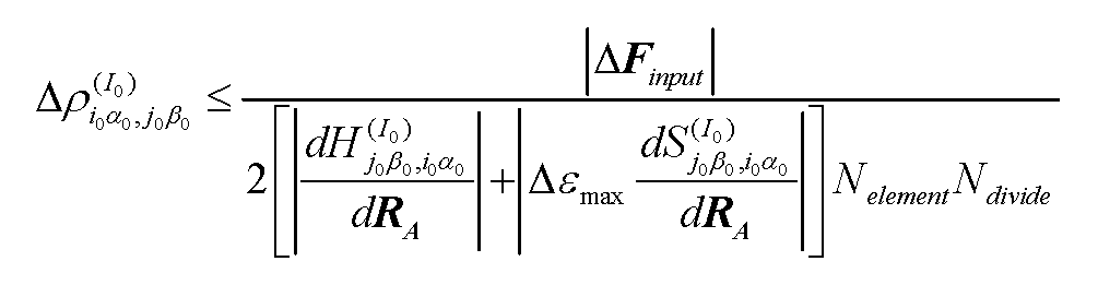
を含む請求項1記載のプログラム。 - 前記第1の数の初期値についての第1の密度行列と前記第1の数の初期値に1を加えた値についての第2の密度行列との差の行列における前記所定の特徴行列要素の値が、前記基準値以下であれば前記探索ステップにおいて前記第1の数を増加させ、前記基準値を超える場合には前記探索ステップにおいて前記第1の数を減少させる
請求項1乃至3のいずれか1つ記載のプログラム。 - 物理量を計算すべき範囲を分割することによって得られる複数の領域に各々設定すべきバッファ領域の原子層数を決定するバッファ領域決定方法であって、
前記複数の領域の各々について、前記バッファ領域の原子層数が第1の数である場合における第1の密度行列と、前記バッファ領域の原子層数が前記第1の数とは異なる第2の数である場合における第2の密度行列との差の行列を算出し、データ格納部に格納する差行列算出ステップと、
前記第1の数を変化させつつ前記差行列算出ステップを繰り返し実行させることにより、前記データ格納部に格納されている前記差の行列における所定の特徴行列要素の値が、指定された物理量から算出される基準値以下である最小の原子層数を探索する探索ステップと、
を含み、コンピュータにより実行されるバッファ領域決定方法。 - 物理量を計算すべき範囲を分割することによって得られる複数の領域に各々設定すべきバッファ領域の原子層数を決定する情報処理装置であって、
データ格納部と、
前記複数の領域の各々について、前記バッファ領域の原子層数が第1の数である場合における第1の密度行列と、前記バッファ領域の原子層数が前記第1の数とは異なる第2の数である場合における第2の密度行列との差の行列を算出し、前記データ格納部に格納する差行列算出処理を実施し、前記第1の数を変化させつつ前記差行列算出処理を繰り返し実行することにより、前記データ格納部に格納されている前記差の行列における所定の特徴行列要素の値が、指定された物理量から算出される基準値以下である最小の原子層数を探索する探索処理部と、
を有する情報処理装置。
Priority Applications (1)
| Application Number | Priority Date | Filing Date | Title |
|---|---|---|---|
| PCT/JP2010/073100 WO2012086023A1 (ja) | 2010-12-22 | 2010-12-22 | バッファ領域決定方法、プログラム及び情報処理装置 |
Applications Claiming Priority (1)
| Application Number | Priority Date | Filing Date | Title |
|---|---|---|---|
| PCT/JP2010/073100 WO2012086023A1 (ja) | 2010-12-22 | 2010-12-22 | バッファ領域決定方法、プログラム及び情報処理装置 |
Publications (1)
| Publication Number | Publication Date |
|---|---|
| WO2012086023A1 true WO2012086023A1 (ja) | 2012-06-28 |
Family
ID=46313327
Family Applications (1)
| Application Number | Title | Priority Date | Filing Date |
|---|---|---|---|
| PCT/JP2010/073100 Ceased WO2012086023A1 (ja) | 2010-12-22 | 2010-12-22 | バッファ領域決定方法、プログラム及び情報処理装置 |
Country Status (1)
| Country | Link |
|---|---|
| WO (1) | WO2012086023A1 (ja) |
-
2010
- 2010-12-22 WO PCT/JP2010/073100 patent/WO2012086023A1/ja not_active Ceased
Non-Patent Citations (3)
| Title |
|---|
| MASATO KOBAYASHI ET AL.: "Implementation of Divide-and-Conquer (DC) Electronic Structure Code to GAMESS Program Package", JOURNAL OF COMPUTER CHEMISTRY, vol. 8, no. 1, 2009, pages 1 - 12 * |
| TAISUKE OZAKI: "Generalized divide-conquer method for large-scale 0(N) DFT calculations", ABSTRACTS OF THE MEETING OF THE PHYSICAL SOCIETY OF JAPAN, vol. 60, no. 1, 4 March 2005 (2005-03-04) * |
| TETSUYA KAWASAKI ET AL.: "A Divide and Conquer Method for Solving Boundary Value Problems based on Shwartz's Alternating Method", IEICE TECHNICAL REPORT, vol. 95, no. 371, 17 November 1995 (1995-11-17), pages 1 - 6 * |
Similar Documents
| Publication | Publication Date | Title |
|---|---|---|
| Liu et al. | Data-driven self-consistent clustering analysis of heterogeneous materials with crystal plasticity | |
| Casula et al. | Size-consistent variational approaches to nonlocal pseudopotentials: Standard and lattice regularized diffusion Monte Carlo methods revisited | |
| Belytschko et al. | On XFEM applications to dislocations and interfaces | |
| Fritzen et al. | Nonlinear reduced order homogenization of materials including cohesive interfaces | |
| Barros et al. | Efficient and accurate simulation of dynamic dielectric objects | |
| Glick et al. | Cartesian message passing neural networks for directional properties: Fast and transferable atomic multipoles | |
| US20100049489A1 (en) | Flow simulation method, flow simulation system, and computer program product | |
| Krekeler et al. | Adaptive resolution molecular dynamics technique: Down to the essential | |
| Borg et al. | The FADE mass-stat: a technique for inserting or deleting particles in molecular dynamics simulations | |
| Xu et al. | A linearly-independent higher-order extended numerical manifold method and its application to multiple crack growth simulation | |
| Zöllner | Grain microstructural evolution in 2D and 3D polycrystals under triple junction energy and mobility control | |
| Wang et al. | Improved Moving Particle Semi-implicit method for multiphase flow with discontinuity | |
| Bzowski et al. | Application of statistical representation of the microstructure to modeling of phase transformations in DP steels by solution of the diffusion equation | |
| Samanta et al. | Exploring the free energy surface using ab initio molecular dynamics | |
| Burczyński et al. | Intelligent optimal design of spatial structures | |
| Gera et al. | Three-dimensional multicomponent vesicles: dynamics and influence of material properties | |
| Beckett et al. | An r-adaptive finite element method for the solution of the two-dimensional phase-field equations | |
| Lin et al. | On the use of a weak-coupling thermostat in replica-exchange molecular dynamics simulations | |
| Richeton et al. | Misorientation dependence of the grain boundary migration rate: role of elastic anisotropy | |
| Cheluvaraja et al. | Thermal nanostructure: An order parameter multiscale ensemble approach | |
| WO2012086023A1 (ja) | バッファ領域決定方法、プログラム及び情報処理装置 | |
| Křišťan et al. | Interactions of glide dislocations in a channel of a persistent slip band | |
| Schlüter et al. | A Lattice Boltzmann method for elastic solids under plane strain deformation | |
| Wallat et al. | Phase-field-based structural optimization of 3D cross-lattice structure to lightweight periodic lattice cells | |
| LeBlanc et al. | Modelling and animation of impact and damage with smoothed particle hydrodynamics |
Legal Events
| Date | Code | Title | Description |
|---|---|---|---|
| 121 | Ep: the epo has been informed by wipo that ep was designated in this application |
Ref document number: 10861037 Country of ref document: EP Kind code of ref document: A1 |
|
| NENP | Non-entry into the national phase |
Ref country code: DE |
|
| 122 | Ep: pct application non-entry in european phase |
Ref document number: 10861037 Country of ref document: EP Kind code of ref document: A1 |
|
| NENP | Non-entry into the national phase |
Ref country code: JP |