WO2004083451A1

WO2004083451A1 - Analysis method

Info

Publication number: WO2004083451A1
Application number: PCT/AU2004/000327
Authority: WO
Inventors: Mervyn Thomas; Harri Kiiveri; David Mitchell
Original assignee: Commonwealth Scientific and Industrial Research Organization CSIRO
Current assignee: Commonwealth Scientific and Industrial Research Organization CSIRO
Priority date: 2003-03-17
Filing date: 2004-03-17
Publication date: 2004-09-30
Anticipated expiration: 2005-09-17
Also published as: AU2003901196A0

Abstract

A method of determining a signature indicative of an entity having a condition, the method comprising the steps of: (a) obtaining at least two distinct data sets, at least one of the data sets containing information on at least one characteristic of at least one entity having the condition; and (b) processing the information from the data sets to obtain a signature that is indicative of an entity having the condition.

Description

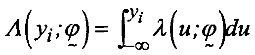
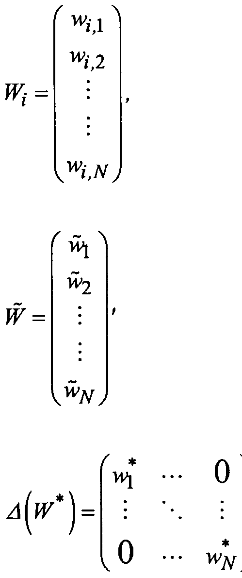
ANALYSIS METHOD

The invention relates to a method and apparatus for identifying a signature indicative of an entity having a condition and for using the signature to identify entities having that condition. The invention has been developed especially, but not exclusively, for identifying samples having a desired therapeutic or biological property and the invention is herein described in that context. However, it is to be appreciated that the invention has broader application and may be used in other complex areas, such as financial modelling and the like.

BACKGROUND OF THE INVENTION

In many systems, the screening of entities for those having a particular condition can be time consuming and expensive. This is especially the case if the entity is one of a large number of entities, or the number of tests that need to be applied to assess whether the entity has a condition are many and/or are expensive. This is especially problematic in applications where large amounts of data are produced for each entity.

An example of an application in which large amounts of data are produced for each entity is in drug discovery. Drug discovery involves the screening of thousands of compounds in a plurality of systems to determine which compounds have a therapeutic or biologically active property. Each system of the drug discovery process generally provides information about one particular characteristic of the compound such as, for example, a chemical or physical property, a gene or protein expression profile in a particular tissue or cell line in response to the compound, enzyme kinetic properties for a particular enzyme or group of enzymes in response to the compound etc. However, the information obtained about each characteristic does not provide sufficient information to make predictions about the ultimate therapeutic or biological properties of the compound.

Typically, the drug discovery process involves screening many thousands of compounds initially in order to identify a single compound having a desired property. With each successive test, compounds which do not exhibit the property sought in each system are eliminated. Thus, by the time the compounds are assessed in a plurality of systems, many thousands of compounds are reduced down to one or a few.

The drug discovery process generally begins with many compounds (either naturally occurring compounds, or synthetically derived compounds such as those generated using methods such as combinatorial chemistry) . The compounds are subjected to a plurality of systems such as biological and chemical analysis, enzymology, genomics and proteomics to mass screen compounds for desired properties in each system (e.g. high efficacy, low toxicity, high stability) . Those compounds identified as having desired properties, known as lead compounds, are then subjected to preclinical testing which may include, for example, pharmacological target testing, formulation and stability testing, and assessment of the compounds ability to be absorbed, distributed, metabolised and excreted (ADME) in test animals. Those lead compounds that exhibit the desired property in the preclinical testing then proceed to clinical testing. Clinical testing is conducted in three phases (I, II and III) .

Phase I clinical testing assesses the tolerance, pharmacological effects, absorption, distribution, metabolism and excretion (ADME) in approximately 20-80 healthy human volunteers. Phase II clinical testing is conducted on 100-300 patients which have the targeted medical condition to determine the effectiveness of treating the medical condition. Phase III is conducted on approximately 1,000-5,000 subjects to determine clinical benefit and incidence of adverse reaction. Following a successful phase III clinical trial, the compound and the results of the clinical trial must be approved by regulatory bodies before the drug is allowed to enter the market .

The total cost of conducting the process from synthesising a compound to reaching the market has been estimated to be approximately US$800 million per compound and can take 15 years or more for a screening of 5,000 to 10,000 compounds. Of these 5,000 to 10,000 compounds, 250 may enter preclinical testing, and of these only 5 survive to enter clinical testing. The screening process to identify lead compounds and precinical testing of these lead compounds account for approximately 36% of the entire cost of drug development .

Clearly, there is a need for a method that is capable of identifying compounds which are more likely to exhibit a desired property than other compounds using a reduced number of test systems and/or reduced amount of data. SUMMARY OF THE INVENTION

In a first aspect, the invention provides a method to determine a signature indicative of an entity having a condition, comprising the steps of;

(a) obtaining at least two distinct data sets, at least one of the data sets containing information on at least one characteristic of at least one entity having the condition; and

(b) processing the information from the data sets to obtain a signature that is indicative of an entity having the condition.

An advantage of the present invention is that it draws on more than one data set to generate a signature of the condition. Each data set may be derived from a system and may include a massive amount of data. In contrast to existing techniques of screening that uses successive tests in isolation to screen for a condition in a target, the present invention is better able to isolate condition signatures because it is able to evaluate relationships between data sets as well as relationships within data sets.

In the context of the present invention, a "signature" is a subset of one or more of the sets of data that is indicative of a condition. Also in the context of the specification, a "system" means a process or arrangement that obtains data is some organised way. The system may be any test, trial, experiment, analysis, measurement or assessment which provides in an organised way that is relevant to a characteristic of the entity. In areas of drug discovery, a system may be a chemical or biological system.

The distinct data sets may be related or unrelated data sets. The distinct data sets may be related in that they contain information about the same characteristic of the entity, but the information is obtained in different ways. Alternatively, the distinct data sets may be obtained using different systems but contain information on the same characteristic. For example, in the context of drug discovery, two distinct data sets may be values for a characteristic such as gene expression in response to a sample in which one data set is obtained by analysing a microarray containing DNA or RNA. It is also envisaged that microarray technologies could be used to measure genetic variations, for example, single nucleotide polymorphisms .

The distinct data sets may be obtained using the same systems but in a different way. For example, using a microarray containing DNA in which gene expression in response to a sample is obtained from different cell lines .

The distinct data sets may be unrelated in that each data set is obtained from different systems, and the information of each data set is on a different characteristic .

The characteristic may be any characteristic of the entity. For example, where the entity is a compound for therapeutic or biological use, the characteristic may be physical or chemical properties of the compound, or biological properties such as, for example, gene expression profile or protein expression profile or antibody binding profile.

Preferably, the information in the data sets relates to components of a system. For example, in the case of a system such as IR-spectrum analysis, the components may be the individual IR spectrum values, or where the system is a DNA microarray, the components may be genes.

The signature that is indicative of the condition may come from data in only one of the data sets, or from any combination of data sets. As such, the signature may be based on one or more characteristics of the entity. In one embodiment, the signature is data generated by a subset of the components of at least one characteristic. Preferably, the subset of components is a minimum number of components that is indicative of the condition.

In one embodiment, the processing step includes using a multivariate analysis to obtain the signature that is indicative of the condition.

Preferably, the multivariate analysis comprises the steps of:

(a) assigning a weight to each component of the data sets;

(b) defining a function of the data and the weights which models the relationship between the condition and the components; (c) applying an algorithm to update the weights using the function in (b) so as to generate a processed weight for each component;

(d) generating a processed data set containing components having a processed weight with absolute value above a predetermined threshold.

Preferably, an assumption is made in setting the assigned weights. The assumption may be any assumption made about the data. In one embodiment, the assumption is a penalty. Preferably, the penalty is a prior assumption. Preferably, the prior assumption is a prior distribution.

Preferably, the multivariate analysis is iterative, with steps (c)and(d) being repeated using the processed data sets in a subsequent cycle of the analysis. In the analysis, the processed weights are used as a basis to establish the assigned weight for the subsequent cycle. As such, the analysis comprises the further steps of;

(a) assigning weights to the components of a said processed data set;

(b) applying the algorithm to fit the weighted data to the function so as to generate a revised processed weight

for each component; (c) generating a revised processed data set containing components having a revised processed weight above a predetermined threshold; , (d) repeating steps (a) to (c) .

Preferably, steps (a) to (c) are repeated until the processed weights remain constant to within a set tolerance with each repeat of steps (a) to (c) . Preferably, the weighted data is in the form of a combination, most preferably a linear combination.

The function is typically a mathematical model of the condition. Preferably, the mathematical model is a model of the distribution of the condition. Preferably, the model of the distribution is a model of the probability distribution of the condition. The model of the probability distribution is preferably a likelihood function.

Preferably, the multivariate analysis estimates component weights utilising a Bayesian statistical method. Preferably, where the at least two distinct data sets comprise a large amount of data, the method preferably makes an a priori assumption that the majority of the data is unlikely to be data that will form part of the signature that is indicative of the condition. The assumption is therefore made that the majority of weights are likely to be zero. A model is constructed which, with this assumption in mind, allows the algorithm to set the weights so that the posterior probability of the processed weights is maximised. The process is iterated until the processed weights remain constant. This method is quick, mainly because of the a priori assumption which results in rapid elimination of the majority of the components.

In one embodiment, the likelihood function is based on a multinomial or binomial logistic regression. The binomial or multinomial logistic regression preferably models a condition of the entity that exhibits a multinomial or binomial distribution. A binomial distribution is a statistical distribution having two possible classes or groups such as an on/off state. Examples of such groups include dead/alive, improved/not improved, depressed/not depressed. A multinomial distribution is a generalisation of the binomial distribution in which a plurality of classes or groups are possible for each of a plurality of entities, or in other words, an entity may be classified into one of a plurality of classes or groups. Thus, by defining a likelihood function based on a multinomial or binomial logistic regression, it is possible to identify a signature that is capable of classifying an entity into one of a plurality of pre-defined groups or classes. For example, the results from microarray data may be classified into pre-defined groups. To do this, samples are grouped into a plurality of sample groups (or "classes") based on a predetermined property of the samples in which the members of each sample group have a common property and are assigned a common group identifier. A likelihood function is formulated based on a multinomial or binomial logistic regression conditional on the linear combination (which incorporates the data generated from the grouped samples) . The condition may be any desired classification by which the results are to be grouped. For example, the property for classification of a chemical compound in a mouse model based on data generated from microarray experiments may be no toxicity, low toxicity, medium toxicity or high toxicity.

Preferably, the likelihood function based on the logistic regression is of the form:

wherein xj β_g is a linear combination generated from input data from training sample i with component weights β_g; x is the components for the i^th Row of X and β_g is a set of component weights for sample class g; and

X is data from n training samples comprising p components.

In another embodiment, the likelihood function is based on an ordered categorical logistic regression. The ordered categorical logistic regression models a binomial or multinomial distribution in which the classes are in a particular order (ordered classes such as for example, classes of increasing or decreasing disease severity) . By defining a likelihood function based on an ordered categorical logistic regression, it is possible to identify a signature that is capable of predicting a result class wherein the class is one of a plurality of predefined ordered classes. By defining a series of group indentifiers in which each group identifier corresponds to a member of an ordered class, and grouping the training samples into one of the ordered classes based on a predetermined condition , a likelihood function can be formulated based on a categorical ordered logistic regression which is conditional on the linear combination (which incorporates the data generated from the grouped training samples) .

Preferably, the likelihood function based on the categorical ordered logistic regression is of the form:

Wherein

Yi_k is the probability that data from training sample i belongs to a class with identifier less than or equal to k (where the total of ordered classes is G ) and rik is defined in Section B below.

In another embodiment of the present invention, the likelihood function is based on a generalised linear model for the condition. The generalised linear model preferably models a condition that is distributed as a regular exponential family of distributions. Examples of regular exponential family of distributions include normal distribution, Gaussian distribution, poisson distribution, gamma distribution and inverse gamma distribution. Thus, in another embodiment of the method of the invention, a signature is identified that is indicative of a predefined condition of a sample that lies within a regular exponential family of distributions by defining a generalised linear model which models the condition to be predicted. Examples of a condition that may be predicted using a generalised linear model include any quantity of a sample that exhibits the specified distribution such as, for example, the weight, size or other dimensions or quantities of a sample.

Preferably, the generalised linear model is of the form:

}

where y = (yi,..., y_n)^τ and aι(φ) = φ /wi with the wi being a fixed set of known weights and φ a single scale parameter. Further details are discussed in Section C below.

In another embodiment, the method of the present invention may be used to predict the time to an event for an entity by utilising a likelihood function based on a hazard model which preferably estimates the probability of a time to an event given that the event has not taken place at the time of obtaining the information. In one embodiment, the likelihood function is based on a model selected from the group consisting of Cox's proportional hazards model, parametric survival model and accelerated failure times model. Cox's proportional hazards model permits the time to an event to be modelled on a set of components and component weights without making restrictive assumptions about time. The accelerated failure model is a general model for data consisting of survival times in which the component measurements are assumed to act multiplicatively on the time-scale, and so affect the rate at which an individual proceeds along the time axis. Thus, the accelerated survival model can be interpreted in terms of the speed of progression of, for example, disease. The parametric survival model is one in which the distribution function for the time to an event in a second system (eg survival time) is modelled by a known distribution or has a specified parametric formulation. Among the commonly used survival distributions are the Weibull, exponential and extreme value distributions.

Preferably, a signature capable of predicting a condition that involves a time to an event is identified by defining a likelihood based on Cox's proportional hazards model, a parametric survival model or an accelerated survival times model, which comprises measuring the time elapsed for a plurality of samples from the time the sample is obtained to the time of the event.

Preferably, the likelihood function for predicting the time to an event is of the form:

N Log (Partial) Likelihood = V g,- 1 β, φ; X, y, c

where β = [β\, 2>'"> p ) ^an<i Ψ ⁼ {^<Pl>P2_''"_' ^<Pq ) ^{are ne} model parameters .

Preferably, the likelihood function based on Cox's proportional hazards model is of the form:

where β^T = (β_\,β₂> - >β_n) , Zj = the j^th row of Z, and ^_j - {'•"' ⁼ ϊ> J^r+!.^•••. N} = ^tne risk set at the j^th ordered event time t(_j\ .

Preferably the likelihood function based on the Parametric Survival model is of the form:

where μ_t = .The notation used in the above

proportional hazards models is explained further in Section D below.

For any defined models, the weights are typically estimated using a Bayesian statistical model (Kotz and Johnson, 1983) in which a posterior distribution of the weights is formulated which combines the likelihood function and a prior distribution. The processed weights are estimated by maximising the posterior distribution of the weights given the data generated for each entity. Thus, the objective function to be maximised consists of the likelihood function based on a function for the condition as discussed above and a prior distribution for the weights.

Preferably, the prior distribution is of the form:

wherein v is a p x 1 vector of hyperparameters, and where plβ v²) is N[θ,diag|v²}) and p(v²) is some hyperprior distribution for v². This hyperprior distribution (which is preferably the same for all embodiments of the method) may be expressed using different notational conventions, and in the detailed description of the preferred embodiments (see below) , the following notational conventions are adopted merely for convenience for the particular preferred embodiment.

As used herein, when the likelihood function for the probability distribution is based on a multinomial or binomial logistic regression, the notation for the prior distribution is:

where β^T =(β ,...β^) and τ^τ =(τ ,...,τ_G ^τ__l).

and piβ_{g g}) is NIO,diag{τ²J) and R(^_g ) s some hyperprior

distribution for T„

As used herein, when the likelihood function for the probability distribution is based on a hazard model , the notation for the prior distribution is:

where β ,β₂,-- -,β_n are component weights, Piβ^τ is N( 0,τ₍ ²1 and

P τ_i I some hyperprior distribution for Ti.

As used herein, when the likelihood function for the distribution is based on a generalised linear model, the notation for the prior distribution is:

wherein v is a p x 1 vector of hyperparameters, and where p(β is some prior distribution

for v².

As used herein, when the likelihood function for the distribution is based on a ordered categories model, the notation for the prior distribution is:

where p(β^* \v² ) is N(θ,diag|v²}] and Py ) some hyperprior

distribution for v² .

As used herein, when the likelihood function for the distribution is based on a hazard model, the notation for the prior distribution is:

where

is Nl0,diag[τ²]) and p(τ) some hyperprior

distribution for V²

The prior distribution preferably comprises a hyperprior that ensures that zero weights are preferred whenever possible.

Preferably, the hyperprior is a Jeffrey's prior.

As discussed above, the prior distribution and the likelihood function are combined to generate a posterior distribution. The posterior distribution is preferably of the form:

or

wherein Lly \β,φ\ is the likelihood function.

The algorithm fits the model to the data by adjusting the weights to maximise the probability density of the posterior distribution of the function. The algorithm may be any algorithm capable of fitting the data to the model by adjusting the weights. The algorithm may be an iterative procedure or an optimisation procedure. Examples of optimisation procedures include genetic algorithms, annealing algorithms, Newton algorithms. Examples of iterative algorithms include gradient descent algorithm, EM algorithm, simplex algorithm, Fletcher- Powell algorithm, conjugative gradients.

The processed weights in the posterior distribution are preferably estimated in an iterative procedure. During the iterative procedure, processed weights having a value less than a pre-determined threshold are eliminated, preferably by setting those weights to zero. This results in elimination of the corresponding component.

Preferably, the iterative procedure is an EM algorithm. The EM algorithm produces a sequence of weight estimates that converge to give processed weights that maximise the probability density of the posterior distribution. The EM algorithm consists of two steps, known as the E or Expectation step and the M, or Maximisation step. In the E step, the expected value of the log-posterior function conditional on observed data and the linear combination is determined. In the M step, the expected log-posterior function is maximised to give updated weight estimates that increase the likelihood. The two steps are alternated until convergence of the E step and the M step is achieved, or in other words, until the expected value and the maximised value of the log-likelihood function converge .

The at least one entity having the condition is preferably one of a plurality of entities having a known condition which are used to "train" the processing step to obtain a signature. Thus, the at least one entity is preferably one of a plurality of entities from which at least two distinct data sets are obtained, at least one of which contains information about at least one characteristics of at least one entity having the condition. Preferably, the plurality of entities comprises one or more entities that have the condition and one or more entities that do not have the condition.

It is envisaged that the method of the present invention may be used in virtually any application to determine a signature indicative of an entity having a condition. The inventors envisage that the method may be used in applications such as drug development (e.g. drug discovery pipeline) , quantitative trait loci analysis for genetic identification or selection of desired phenotypes, financial analysis and/or financial prediction such as stock prediction based on various financial and non- financial parameters (components) , manufacturing in, for example, efficiency management or prediction of product failure, market analysis to predict desired outcomes in product sales or target markets, sport for the prediction of outcomes in competition, weather for the prediction of a particular outcome in a particular geographic region. The entity may be anything for which a condition is sought and which has at least two characteristics. For example, if the method of the invention is used to determine a signature that is indicative of the share price of a company (the condition) , the entity may be a company. The characteristics of the company may be, for example, account figures, stock prices of other companies, employee numbers, market estimates, or any other information that may be relevant to the price of shares of the company. In another example, the entity may be a particular city and the condition may be rainfall. The characteristics relevant to the city may be rainfall in other cites around the world, humidity in other cites around the world or any other information that may be relevant to the rainfall in that particular city. In one embodiment, the entity is a sample. Preferably, the sample is a compound. Preferably, the compound is synthesised or naturally occurring.

It will be apparent to persons skilled in the art that the condition of the entity will depend on the nature of the entity and the use for which the entity is intended. Preferably, the condition may be a property of the entity. Preferably, the property is a desired property of the entity. For example, if the entity is a compound and the use is for treatment of a disease, then the condition may be, for example, the ability to alleviate symptoms of the disease, or low toxicity, or ability to bind a drug target. If the entity is a company, then the condition may be, for example, a 10% rise in share price.

It is envisaged that the condition may be that the entity will produce a data set in at least one further system. The data set produced in the further system may comprise a signature that is indicative that the entity has a further condition. Thus, the method of the present invention may be used to determine a signature that is indicative of a signature in a further at least one system, wherein the signature is indicative of a further condition.

Once a signature is identified using the method of the invention, the signature may then be used to identify an entity having the condition.

Thus, in a second aspect, the invention provides a method for determining whether a test entity has a condition comprising the steps of:

(a) determining a signature indicative of the condition in accordance with the first aspect; and

(b) obtaining data about a test entity;

(c) determining whether the information about the test entity contains data equivalent to the signature, to determine whether the test entity has the condition.

It will be appreciated by those skilled in the art that in determining whether a test entity has a condition, only those components from which data for the signature is obtained need be considered. Thus, the amount of data that is generated may be greatly reduced.

Also contemplated are computer programs, apparatus and systems for determining a signature that is indicative of an entity having a condition from at least two distinct data sets containing information on at least one characteristic of at least one entity having the condition.

In a third aspect, the invention provides a computer program, arranged, when run on a computing device, to control the computing device to process information from at least two distinct data sets, at least one of the data sets containing information on at least one characteristic of at least one entity having a condition, to obtain a signature that is indicative of the condition of an entity having the condition.

The computer program may implement any of the preferred algorithms and method steps of the processing steps which are discussed above.

Preferably, the computer program is provided on a computer readable medium.

The computer program may be arranged to implement any of the preferred method and calculation steps discussed above in relation to the processing steps.

In a fourth aspect, the invention provides an apparatus for processing information from at least two distinct data sets, at least one of the data sets containing information on at least one characteristic of at least one entity having a condition, to obtain a signature that is indicative of the condition of an entity having the condition. In a fifth aspect, the invention provides a system which is arranged to identify data obtained from processing information from at least two distinct data sets, at least one of the data sets containing information on at least one characteristic of at least one entity having a condition, to obtain a signature that is indicative of the condition of an entity having the condition, the system comprising a user interface and a storage means arranged to store a processing template, the template including pre-stored model parameters for controlling the system in accordance with the parameters and wherein a user is able to select the processing template via the interface and the system is arranged to carry out processing of the information from at least two characteristics in accordance with the model parameters.

Where aspects of the present invention are implemented by way of a computing device, it will be appreciated that any appropriate computer hardware e.g. a PC or a mainframe or a networked computing infrastructure, may be used.

In a sixth aspect of the present invention, there is provided a method of determining whether a substance has a potential for use as a drug, the method comprising the steps of: obtaining a first mathematical model that is derived using a signature of a condition of an entity; using the first mathematical model in conjunction with information about at least one characteristic of another entity that has been exposed to the substance; and using a result from the first mathematical model to determine whether the substance has the potential for use as the drug. Preferably, the signature is obtained using the method as described in the first aspect of the present invention.

Preferably, the method further comprising the step of selecting the substance from a plurality of substances by using a second mathematical model in conjunction with other information about the plurality of substances.

Preferably, the first mathematical model is such that the result represents a probability that the substance is not toxic to the other entity.

Preferably, the second mathematical model is such that it represents a toxicity measurement for the substance in relation to the other entity.

The apparatus of the third aspect preferably includes an appropriately programmed processor for implementing the method steps.

BRIEF DESCRIPTION OF THE DRAWINGS

Figure 1 illustrates a schematic diagram of a preferred embodiment in which two data sets are used to identify a signature that is indicative of low toxicity in mice.

Figure 2 illustrates a schematic diagram of a preferred embodiment in which a many data sets are used to identify a signature that is indicative of a condition. Figure 3 illustrates a flow diagram of an embodiment of the method of the present invention showing the steps in processing the data sets.

Figures 4 to 6 illustrate flow diagrams of the various steps carried out in the preferred embodiment of the present invention.

DETAILED DESCRIPTION OF THE PREFERRED EMBODIMENT

The method of the invention may be used to determine a signature indicative of a sample having a desired property from data generated from a plurality of training samples.

In a preferred embodiment, the invention provides a method for determining a signature that is indicative of whether a test sample has a desired property, the method comprising the steps of:

(a) Obtaining distinct data sets containing information on at least one characteristic of a training sample, the data sets being obtained from a plurality of training samples, each applied to a plurality of systems, wherein one or more of the training samples have the desired property;

(b) using multivariate analysis of the information from the data sets to obtain a signature that is indicative of a training sample having the desired property.

This embodiment of the invention permits identification of a signature that is indicative of whether a sample has a desired property by utilising training samples applied to a plurality of systems to identify a signature that is indicative of the desired property. Preferably, the signature is data generated from a subset of components of the characteristic. The method utilises training samples having a known condition in order to identify a signature for a subset of components which is indicative of a desired feature for a training sample having the desired feature. Subsequently, knowledge of the subset of components can be used for test samples to determine whether the test samples have the desired property. In future screenings for samples having the desired property, it is necessary only to measure the subset of components to determine whether a test sample has the desired property.

In another embodiment, the invention therefore provides a method for determining whether a test sample has a desired property, comprising the steps of:

(a) obtaining test data from the test sample;

(b) determining the signature value for the test sample, to thereby determine whether the test sample has a desired property.

In a particularly preferred embodiment, the method of the present invention is used to identify compounds which are capable of producing a therapeutically desirable effect in, for example, humans or animals (test system) based on the data generated from a plurality of systems such as, for example, a combination of mass spectrometry, array analysis and proteomic analysis of the sample.

As discussed above, the signature may be data corresponding to components of the system. Components are preferably any measurable elements that may be: (a) part of a sample; or (b) part of a system and which are responsive to a sample being applied to the system. For example, components that may be considered part of, or result from, a sample that is, for example, a chemical compound may be NMR chemical shifts values, UV-VIS absorbance values, reaction constant values, equilibrium constants values, solubility constant values. Examples of components that may be part of a system which are responsive to a sample being applied to the system include for example, expression levels for genes or proteins from a cell type that are produced in response to a sample being applied to that cell type. The expression levels may be determined by, for example, microarray analysis.

The method of the present invention may be performed on information about a characteristic without any prior knowledge of the characteristic. There is no requirement that the charactistic or components of the characteristic be known or that the mechanisms underlying the characteristic be understood. The only requirement is that each component has a unique identifier which permits each data value for that information to be assigned to a component. Thus, characteristics may be used in the method of the invention which are not well characterised or understood, and/or are extremely complex and/or generate large amounts of data. In fact, the method of the present invention works efficiently with huge amounts of information about a characteristic and/or when the information is extremely complex and in which high variability of the information is common.

As used herein, the term "signature" refers to a subset of data obtained from processing of at least two distinct data sets. Preferably, the signature is data values for a subset of components of one or more systems. The range of data values of the signature may vary depending on the data that is analysed, the multivariate analysis that is applied, and the system to which the sample is applied. Preferably, the signature tolerates a high level of variation in which the test data may differ widely from the training data for the subset of components but may still be indicative of the desired property.

As used herein, the term "training samples" refers to samples which are known to either have or produce the desired property, or not have or not produce the desired property. Thus, the training samples are preferably one of the following two types:

(a) those that are have or acapable of producing the desired property; or

(b) those that are do not have or are not capable of producing the desired property.

Preferably, the data generated from the multivariate analysis is "predictive" of whether a sample has or can produce a desired property. Essentially, from all the data that is generated from the plurality of systems, the method of the present invention enables identification of a minimum number of components that can be used to predict whether a sample has a particular desired property. The training samples are thus used to identify the subset of components capable of predicting the desired property of a sample. Once those components have been identified using the training samples, only the subset of components need be used in future to assess test samples. Because a subset of components is identified that are predictive of a desired property, only the subset of components need be measured during the screening of test samples. Thus, the method of the present invention permits test samples that are likely to have a desired property to be identified without the need to measure all the components of the plurality of systems in response to the test sample.

In one embodiment, the distinct data sets from the plurality of systems are combined prior to processing. In other words, the signature is generated from the combined training data from the plurality of systems. The multivariate analysis is thus applied to the combined training data from the plurality of systems in one step to generate a subset of components identified from all the information from all the systems.

In another embodiment, the data sets from the plurality of systems are processed successively. In this way, a signature may be determined from a data set from a first system that is predictive of a desired result in a second system. The desired result in the second system may be that the data generated from the second system has a particular signature that is predictive of a desired result in a third system of the plurality of systems. Thus, by obtaining a signature from a data set that relates to another data set, it is possible to identify a signature that is predictive of a desired property from successive systems.

The order of the successive systems may be any order that is appropriate for assessing the test sample (s). Typically, the order is determined by the complexity and/or expense of each system relative to the other screening systems. For example, screening systems of less complexity or expense may be used early in the plurality when there are many samples to be tested, while more complex and/or expensive systems are preferred later in the plurality when many or most of the samples have been eliminated. For example, in drug discovery, systems such as mass spectrometry and infra-red spectrometry generate large amounts of data for each test compound relatively quickly and cheaply, and consequently many compounds may be subjected to this analysis early in the drug screening process. Microarray analysis is a more complex and expensive analysis and is therefore generally used further down the succession of systems where compounds of no interest have been screened out using the previous systems .

The succession of systems may be separated by one or more other systems of the succession of systems, or in other words, the first and second systems need not be consecutive steps in the succession. For example, a typical succession of systems used to identify a compound that is, for example, non-toxic in mammals may be: mass spectrometric analysis, then testing in a series of tissue culture cells, then testing in a series of animal models to determine, for example, toxicity and finally ADME testing. Data generated from, for example, mass spectrometric analysis (the first system) may be used to identify a subset of components that is predictive of a desired property in, for example, ADME testing. Thus, the inventors envisage that the method of the invention will allow some or many systems that are typically required for drug dicovery to be ommitted when screening test samples. In other words, the method may permit "leapfrogging" of systems to increase speed and efficiency of the screening or testing procedures for the desired property.

It is also envisaged that a plurality of data sets may be combined before processing, and that the signature obtained from the combined data may be indicative of a signature in another data set. In this way, a signature may be obtained from data from a one or more systems of a plurality of systems which a predictive of a condition in a system that is also one of the plurality of systems.

The desired property may be any property of the sample that is sought. The desired property may be a direct property of the sample such as for example, when the sample is a compound, a physical or chemical property such as solubility, stability, a particular feature of structure, or a biological property such as toxicity, receptor binding capability, the ability to induce or inhibit gene or protein expression, pharmocological property of the compound such as target interaction. In some cases, the desired property will be readily apparent from a single result such as toxicity, solubility, whereas in other cases the desired property may be contained within a large amount of data, such as a signature that is predictive of a result in a further system.

In one embodiment, the desired property is a signature generated from a subset of components in a further one or more systems. Preferably, the signature generated from a subset of components in a further one or more systems is predictive of a further property. The desired property may be any property or outcome that is sought in relation to the test sample when applied to a system. For example, if the sample is a compound for therapeutic use, the desired property may be, for example, low toxicity in cells, animals, or humans, effectiveness or low toxicity on a particular cell type in cell culture, ability to target a particular gene(s) or protein (s) or other cellular component, ability to induce a particular physiological response, ability to inhibit or kill a particular cell type or infectious agent.

It is also envisaged that the desired property may be data from a subset of components of a further system. Preferably, the data from the subset of components of the further system is predictive of a desired property in another system.

The choice of the plurality of systems will of course depend on the sample that is being tested and the desired property that is sought. For example, if the sample is a compound for drug discovery, the plurality of systems may include one or more chemical and/or biological systems. A biological system may be any system for assessing the chemical interaction that involves molecules of the type found in living organisms. Such interactions include anabolic and catabolic reactions that occur in living organisms including enzymatic reactions, binding reactions, signalling reactions and other reactions. Examples of biological systems include analysis of receptor-ligand interaction, analysis of enzyme-substrate interaction, analysis of cellular signalling pathways, toxicology assays, analysis of gene expression in response to a sample, analysis of protein expression in response to a sample, analysis of the physico-chemical properties of the test sample, analysis of toxicity when the test sample is applied to the system, analysis of the mutagenic potential of a test sample, analysis of ADME. The components may be labelled or organised in a manner which allows data from one component to be distinguished from data from another component. For example, the components may be spatially organised in, for example, an array which allows data from each component to be distinguished from another by spatial position, or each component may have some unique identification associated with it such as an identification signal or tag. For example, the components may be bound to individual carriers, each carrier having a detectable identification signature such as quantum dots

(see for example, Rosenthal, 2001, Nature Biotech 19: 621- 622; Han et al . (2001) Nature Biotechnology 19: 631-635), flourescent markers (see for example, Fu et al , (1999) Nature Biotechnology 17: 1109-1111), bar-coded tags (see for example, Lockhart and trulson (2001) Nature

Biotechnology 19: 1122-1123), or chemical labelling such as that described in US Patent No. 6,475,807. The biological system may be a biotechnology array. Examples of biotechnology arrays include oligonucleotide arrays, DNA arrays, DNA microarrays, RNA arrays, RNA microarrays, DNA microchips, RNA microchips, protein arrays, protein microchips, antibody arrays, chemical arrays, carbohydrate arrays, proteomics arrays, lipid arrays. In another embodiment, the biological system may be selected from the group including, for example, DNA or RNA electrophoresis gels, protein or proteomics electrophoresis gels, biomolecular interaction analysis such as Biacore analysis, amino acid analysis, ADME screening (see for example High-throughput ADME estimation: In Vitro and In Silico approaches (2002) , Ferenc Darvas and Gyorgy Dorman (Eds) , Biotechniques Press) , protein electrophoresis gels and proteomics electrophoresis gels.

Chemical systems may be any system that provides data in relation to the chemical or physical properties of a sample or a system in response to a sample . Examples of chemical systems include atomic absorption spectroscopy (AAS) , auger electron spectroscopy (AES) , coherent anti- Stokes spectroscopy (CARS) , circular dichroism (CD) , Conversion electron Mossbauer spectroscopy (CEMS) , chemical ionisation mass spectroscopy, chemically-induced dynamic electron/nuclear polarisation (CIDEP/CIDNP) , Cross polarisation magic angle spinning (CP-MASS) , combined rotation and multipulse spectroscopy (CRAMPS) , distortionless enhancement by polraisation transfer, 2- Dimensional nuclear magnetic resonance spectroscopy, electron diffraction (ED) , energy dispersive X-ray spectroscopy, electron energy-loss spectroscopy, electron- electron double resonance, electronic spectroscopy, electron impact mass spectroscopy, electron-nuclear double resonance (ENDOR) , electron paramagnetic resonance spectroscopy, electron spin resonance spectroscopy (ESR) , exchange spectroscopy, far infrared laser magnetic resonance, flourescence spectroscopy, Fourier transform infrared spectroscopy (FTIR) , gas-phase electron diffraction (GED) , heteronuclear correlation spectroscopy (HETCOR) , heteronuclear overhauser effect spectroscopy, Hyper Raman spectroscopy, infrared spectroscopy (IR) , laser desorption mass spectroscopy, laser-induced fluorescence, laser magnetic resonance spectroscopy, magnetic circular dichroism, microwave spectroscopy, mass- analysed ion kinetic energy spectroscopy, microwave optical double resonance spectroscopy, Mossbauer spectroscopy, multiphoton ionisation spectroscopy, multistage mass spectroscopy (MS/MS) , multiphoton induced flourescence spectroscopy, nuclear gamma resonance spectroscopy, nuclear overhauser spectroscopy, nuclear quadrupole resonance spectroscopy, optical double resonance spectroscopy, photoelectron spectroscopy, photoionisation mass spectroscopy, Raman spectroscopy, Raman-induced Kerr-effect spectroscopy, rotating frame

Nuclear Overhauser Effect spectroscopy, rotational Raman spectroscopy, Rotational spectroscopy, resonance Raman spectroscopy, secondary ion mass spectroscopy, total correlation spectroscopy, vibrational spectroscopy, visible spectroscopy, X-ray diffraction, X-ray fluorescence spectroscopy, X-ray photoelectron spectroscopy, correlation spectroscopy (COSY) , Coulomb explosion, HPLC, mass spectrometry (for example, MALDI, MALDI-TOF, LC-MS, MS-MS, GC-MS, LC/MS-MS, ES-MS, LC-ES- MS) .

Biological systems may also be used in applications such as quantitative trait loci analysis in animals and humans. For example, tissue samples from plants, animals or humans having known desired and undesired phenotypes may be applied to a plurality of biological systems such as, for example, microarray analysis and PCR-analysis in order to determine a signature, and this signature may be used to identify a subset of genes or loci that are predictive of the plant, animal or human having a desired property such as, for example, physical attributes such as, for example, size, strength, speed, muscle development, fat content, growth rate, breeding capacity, colour, drought resistance, flavour etc. or attributes such as personality, intellectual capacity, or some particular talent such as sporting prowess, musical ability etc.

Any training samples may be used in the method of the invention provided a portion of the training samples have or produce the desired property. Preferably, the training samples produce data with sufficient variability to distinguish between training samples having different properties. In one embodiment, when the plurality of systems is for drug discovery, the training samples may be any chemical or biological compound, either naturally occurring or synthesised. Examples of naturally occurring compounds include nucleic acid, protein, carbohydrate, antibody, glycoprotein, modified protein, lipoprotein, lipid, phospholipid, polysaccharide, organic or inorganic molecule, biological macromolecule, or any other naturally occurring compound which is to be tested for a desired property. Also contemplated are synthesised chemical compounds such as those generated by combinatorial chemistry. Examples of methods for the generation of compounds using combinatorial chemistry include those described in Dower et al . (1991) Ann. Rep. Med. Che. 26:271-280; Fodor et al . (1991) Science 251: 767-773; Jung et al. (1992) Angew. Chem. Ind. Ed. Engl . 31:367-383;

Zuckerman et al . (1992) PNAS 89:4505-4509; Scott et al . (1990) Science 249:386-390; Devlin et al . (1990) Science 249: 404-406; Cwirla et al . (1990) PNAS 87: 6378-6382; Gallop et al . (1994) J. Medicinal Chemistry 37: 1233-1251. It is also envisaged that the test sample may be a mixture of chemical compounds such as those mentioned above. In this regard, it is envisaged that the method of the invention may be used to identify compounds which act synergistically to exhibit a desired property, or identify complex mixtures of compounds such as those found in naturally occurring substances e.g. plant extracts, saps, body fluid extracts which exhibit a desired property, or compounds produced through industrial processes which exhibit a desired property.

The test sample may be any sample for which a desired property is sought. It will be appreciated by those skilled in the art that the test samples may be the same type of compounds as the training samples, or made using the same methods .

In embodiments where the test sample is a compound for which a therapeutic or biological property is sought, it will be appreciated by persons skilled in the art that the classes of chemical that may be used in the method of the invention need not be limited to any particular chemical, and that the method of the invention encompasses the use of any compound as a test sample. For example, the chemical compound may be a nucleic acid, protein, carbohydrate, pharmaceutical, antibody, glycoprotein, modified protein, lipoprotein, lipid, phospholipid, polysaccharide, organic or inorganic molecule, biological macromolecule, or any other naturally occurring or synthesized chemical compound which is to be tested for a desired property. Synthesised chemical compounds such as those generated by combinatorial chemistry are particularly preferred. It is also envisaged that the test sample may be a mixture of chemical compounds such as any of those mentioned above. In this regard, it is envisaged that the method of the invention may be used to identify compounds which act synergistically to exhibit a desired property, or identify complex mixtures of compounds such as those found in naturally occurring substances e.g. plant extracts, saps, body fluid extracts which exhibit a desired property, or compounds produced through industrial processes which exhibit a desired property.

The component may be one or more measurable components of the characteristic. For example, in a biological system the components may be genes, proteins, antibodies, carbohydrates, lipids, phospholipids or any other components of a biological system, and the data generated from the systems is typically a measure of the levels of these components in response to a sample applied to the systems. The components may be known components, or in other words, previously identified components. However, there is no requirement that the components be previously known and consequently the components may be unknown components, or in other words, components that have not been previously identified. It is envisaged that the method of the invention may also be used with a combination of known and unknown components.

The signature may be identified using any multivariate analysis. In one embodiment, the multivariate analysis comprises generating a combination of weighted components to identify a subset of components that provide the signature. A flow diagram of the steps involved in a preferred method of the multivariate analysis is shown in Fig. 3.

Data generated by applying the training samples to the plurality of systems is processed using a multivariate analysis to identify a signature that is capable of correctly predicting whether a training sample has a desired property. The multivariate method used to determine the signature may be any multivariate method capable of handling large amounts of data. Preferably, the multivariate method is a Bayesian method. Preferably, the bayesian method combines a prior, and a likelihood function which models the distribution of the data generated by the training samples. Thus, the type of bayesian method selected in the method of the invention will typically depend on the distribution of the desired property. Most samples having a desired property typically exhibit a probability distribution, and the probability distribution of a desired property can be modelled using statistical models which are based on the data generated from the training samples in the plurality of systems. The method utilises statistical models which model the probability distribution for a desired property. Thus, for a sample having a desired property with a particular probability distribution, an appropriate model is defined that models that distribution. The method preferably uses any model that is conditional on the linear combination, and is preferably a mathematical equation in the form of a likelihood function that provides a probability distribution based on the data obtained from the training samples. Preferably, the likelihood function is based on a previously described model for describing some probability distribution. In one embodiment, the model is a likelihood function based on a model selected from the group consisting of a multinomial or binomial logistic regression, generalised linear model, Cox's proportional hazards model, accelerated failure model and parametric survival model. For example, if the desired property exhibits a binomial or multinomial distribution, then the likelihood function of the Bayesian method correspond to that of a logistic regression. If the desired property exhibits an ordered multiclass distribution, then the likelihood function of the Bayesian method will correspond to that of an ordered categories model. If the desired property exhibits a distribution from the class of generalised linear models , then the likelihood function of the Bayesian method will correspond to that of a generalised linear model. If the desired property is survival data for an animal or human, or measures some type of failure of a system or sample, then the likelihood function of the Bayesian method will correspond to that of a proportional hazards model.

The multivariate method of the preferred embodiment is particularly suited to the analysis of very large amounts of data. Typically, large data sets are often highly variable and test sample data often differ significantly that obtained from the training samples. By using the multivariate methods of the preferred embodiment, it is possible to identify signatures using training samples which can be used to determine whether a test sample has or will have a desired property, even when the data generated from the test sample is highly variable compared to the data generated from training samples having the desired property. Thus, the multivariate method of the preferred embodiment is able to identify a signature that is indicative that a test sample has a desired property even when the data from the test sample is of poor quality and/or there is a high variability between the training samples having the desired property. In fact, the method may preferably select components that exhibit high variability between training samples having the desired property (and yet are predictive of the property) as these components are more likely to be correctly predictive for highly variable test samples. In other words, the method of the present invention is capable of identifying components that have a high tolerance to variation. In this way, the subsets of components are able to predict response characteristics in test data that varies from the training data.

The multivariate method of the preferred embodiment also has the advantage that it requires usage of less computer memory than prior art methods. Accordingly, the method of the present invention can be performed rapidly on computers such as, for example, laptop machines. By using less memory, the method of the present invention also allows the method to be performed more quickly than prior art methods for analysis of, for example, biological data.

Preferred embodiments of the multivariate methods are now described in greater detail .

A. Multi Class Logistic regression model

The multivariate method of this embodiment utilises the training samples in order to identify a signature from at least two distinct data sets which can classify the samples into a pre-defined groups , wherein at least one of the pre-defined groups exhibits the desired property. For example, a set of data from mass spectrometry analysis and microarray analysis generated from a particular training sample may be used to predict that that training sample belongs to a pre-defined group. In this way, the multivariate method identifies preferably a minimum number of components from the data set that can be used to determine that a training sample belongs to a pre-defined group. Thus, when one of the pre-defined groups is a group which exhibits the desired property, the subset of components is therefore indicative that the sample is capable of producing the desired property by classifying the training sample into that group.

Once the subset of components have been identified using the training samples, data for the subset of the components may be obtained using test samples to determine whether that test sample is capable of producing a result in the appropriate system that is in the group having the desired property.

The pre-defined group may be any classification which groups the samples. For example, the samples may be grouped on the basis of particular array results, wherein those samples that produce a pattern of gene expression in the second system belong to a particular group, whether those samples are low toxicity, high efficacy etc. For example, a pattern of gene expression may be for example, a subset of genes that is predictive of the sample producing a desired result in another system.

In one embodiment, the input data is organised into an n x p data matrix X = (x_jj) with n training samples and p components. Typically, p will be much greater than n .

In another embodiment, data matrix X may be replaced by an n x n kernel matrix K to obtain smooth functions of X as predictors instead of linear predictors. An example of the kernel matrix K is ki_j=exp (-0.5* (xi-X_j) ^t (xi-X_j) /σ²) where the subscript on x refers to a row number in the matrix X. Ideally, subsets of the columns of K are selected which give sparse representations of these smooth functions. Further examples of kernel matrices are given in table 2 below.

Associated with each sample class (group) may be a class label y_{ , where y_t = k,k e

which indicates which of G sample classes a training sample belongs to. We write the nxl vector with elements y, as y. Given the vector y we can define indicator variables

^s 0, otherw ⁸ise <^IA>

In one embodiment, the processed component weights are estimated using a Bayesian statistical model (see Kotz and Johnson, 1983) . Preferably, the processed weights are estimated by maximising the posterior distribution of the weights given the data generated from each training sample. This results in an objective function to be maximised consisting of two parts. The first part a likelihood function and the second a prior distribution for the weights which ensures that zero weights are preferred whenever possible. In a preferred embodiment, the likelihood function is derived from a multiclass logistic model. Preferably, the likelihood function is computed from the probabilities: (2A)

and

Wherein

ig is the probability that the training sample with input data X± will be in sample class gr; j β_g is a linear combination generated from input data from training sample i with component weights β₉; x is the components for the i^th Row of X and β_g is a set of component weights for sample class g;

Typically, as discussed above, the processed component weights are estimated in a manner which takes into account the a priori assumption that most of the component weights are zero.

In one embodiment, components weights βg in equation (2A) are estimated in a manner whereby most of the values are zero, yet the samples can still be accurately classified.

In one embodiment, the prior specified for the parameters /?,,...,?_G_, is of the form:

where β^τ = {β! ,...β_G ^τ__λ) and τ^τ = ( ,..., x_G ^τ_ ).

and p(β_g ll τ² _g is a Jeffreys

hyperprior, Kotz and Johnson (1983) .

In one embodiment, the likelihood function is

of the form in equation (8A) and the posterior distribution of β and T given y is

In one embodiment, the first derivative is determined from the following equation:

aiogz

= ^χT k ^~ _g)> g = ;G-l ( 6A) W^g

wherein e_g ^τ = \e_ig,i = l,n , p_g ^τ = (p_ig,i = l,n are vectors indicating membership of sample class g and probability of class g respectively.

In one embodiment, the second derivative is determined from the following algorithm:

3² logZ,

= -X^τdiag {δ_hgPg -p_hp_g}x ( 7A)

Equation 6A and equation 7A may be derived as follows (a) Using equations (1A) , (2A) and (3A) , the likelihood function of the data can be written as:

(b) Taking logs of equation (8A) and using the fact that

G *=^l for all i glves :

Λ=l

(c) Differentiating equation (9A) with respect to βg gives

aiogE

= X^T (e_g - p_g), g = l,...,G -l (10A) dβg

whereby e^ = \e_lg,i = l,nj , p_g = (p_lg,i = l,n) are vectors indicating membership of sample class g and probability of class g respectively.

(d) The second derivative of equation (9A) has elements

_ _{vT j}.

= -X^τdiag [δ_hgPg - p_hPg }X ( 11A)

where

se

Processed component weights which maximise the posterior distribution of the likelihood function may be specified using an EM algorithm comprising an E step and an M step.

Typically, the EM algorithm comprises the steps :

(a) performing an E step by calculating the conditional expected value of the posterior distribution of component weights using the function :

Q= log L -- γ_g ^τ diag[γ_g} γ_g ( 12A)

¹ 8=

where x β

in equation ( 8A)

(b) performing an M step by applying an iterative procedure to maximise Q as a function of γ whereby :

where ' is a step length such that O≤α'≤l; βg = PgYgi wherein P_g are matrices of zeroes and ones such that P^τ _gβ_g selects non-zero elements of β_g; and

Equation (12A) may be derived as follows:

Calculate the conditional expected value of 5A) given the observed data y and a set of parameter estimates β .

Consider the case when components of β (and β ) are set to zero i.e for g = 1,..., G-l, β_g = P_gγ_g and β_g = P_g7_g, where the P_g are matrices of zeroes and ones such that P_g β_g selects the non zero elements of β_g . In the following we write γ = ( γ_g , g=l,...,G-l) . Note that the γ_g are actually subsets of the components of β_g . We use them to keep the notation as simple as possible.

Ignoring terms not involving γ and using (4A) , (5A) , (9A) we get :

l ^G~^l -2

= log L -- γ_g ^τ diag{γ_g} γ_g ( 14A) ^z g=ι

where x β_g = x,^TP_Rf_R in ( 8A) Note that the conditional expectation can be evaluated from first principles given (4A) .

The iterative procedure may be derived as follows:

To obtain the derivatives required in (13A) , first note that from (8A) , (9A) and (10A) we get

and

A_gh=diag{δ_ghPg-p_gp_h}, where

se

and X_g ^T=PX^T,g = l,...G-l. (17A)

In a preferred embodiment, the iterative procedure may be simplified by using only the block diagonals of equation (16A) in equation (13A) . For g = l,...G-l, this gives:

ϊ? =r_g'+cc' {x_g ^TA_ggX_g + diag {γ_g ]*}^"' x_g ^τ (e_g - _Pg)- diag {γ_g}^"2 γ_g' } (18A)

Rearranging equation (18A) leads to

where

Y_g ^τ=diag{γ_g}X_l

Writing p(g) for the number of columns of Y_g , (19A) requires the inversion of a p(g)xp(g) matrix which may be quite large. This can be reduced to an nxn matrix for p{s)^>n by noting that:

where Z_g=Δ_g ² _gY_g. Preferably, (19A) is used when p(g)<n and (19A) with (20A) substituted into equation (19A) is used when p(g)≥n. In a preferred embodiment, the EM algorithm is performed as follows:

1. Set n=0

and choose an initial value for γ°. This is done by ridge regression of log(pi_g/pi_G ) on Xi where Pig is chosen to be near one for observations in group g and a small quantity >0 otherwise - subject to the constraint of all probabilities summing to one.

2. Do the E step i.e evaluate Q =

3. Set t=0. For g — 1,...,G-1 calculate: a) δ_g' =γ_g' ^x -γ_g' using (19A) with (20A) substituted into (19A) when p(g)≥n.

(b) Writing δ' =(δ_g',g = l,...,G-l) Do a line search to find

the value of ' in γ'⁺ⁱ =γ' +a'δ' which maximises (or

simply increases) (12A) as a function of a' . c) set γ'⁺ⁱ=γ' and t=t+l Repeat steps (a) and (b) until convergence.

This produces γ^*"^+x say which maximises the current Q function as a function of γ.

For g = l,...G-l determine

Where ε <κl , say 10^"5. Define P_g so that β_ig= for teS_gand

fT={rT ^_g} This step eliminates variables with small coefficients from the model .

4. Set n=n+l and go to 2 until convergence.

A second embodiment in which a multivariate analysis relating to a categorical ordered logistic regression is used will now be described.

B. Ordered categories model

The multivariate method of this embodiment utilises the training samples in order to identify a signature from a subset of components which can classify the samples into a pre-defined ordered group, wherein at least one of the pre-defined ordered groups exhibits the desired property. The pre-defined ordered group may be, for example, increasing toxicity in cells, or an LD50 experiment.

In the following there are N samples, and vectors such as y, z and μ have components yi, Zi and μi for i = 1,..., N. Vector multiplication and division is defined componentwise and diag{ " } denotes a diagonal matrix whose diagonals are equal to the argument. We also use | | | | to denote Euclidean norm.

Preferably, there are N observations y. where y. takes integer values 1,...,G. The values denote classes which are ordered in some way such as for example severity of disease. Associated with each observation there is a set of covariates (variables, e.g gene expression values) arranged into a matrix X with N rows and p columns wherein

N is the samples and p the components. The notation x₍ denotes the i^th row of X. Individual (sample) i has probabilities of belonging to class k given by n_lk = π_k(x^) .

Define cumulative probabilities

Note that γ_Λ is just the probability that observation i belongs to a class with index less than or equal to k. Let C be a n by p matrix with elements c_y given by

_ f 1, if observation I in classj ij ~ 0, otherwise and let R be an n by P matrix with elements r given by

^rυ =∑^l g=ι These are the cumulative sums of the columns of C within rows .

For independent observations (samples) the likelihood of the data can be written as

and the log likelihood (log(L)) 1 can be written as

The continuation ratio model may be adopted here as follows :

for k = 2,...,G , see McCullagh and Nelder(1989) and McCullagh(1980) and the discussion therein. Note that (4B)

The likelihood is equivalent to a logistic regression likelihood with response vector _yand covariate matrix X y =vec{R}

where/_c_, is the G-l by G-l identity matrix and l_c_. is a G-

1 by 1 vector of ones.

Here vec{ } takes the matrix and forms a vector row by row.

Typically, as discussed above, the component weights are estimated in a manner which takes into account the a priori assumption that most of the component weights are zero.

Following Figueiredo (2001) , in order to eliminate redundant variables (covariates) , a prior is specified for the parameters β by introducing a p x 1 vector of hyperparameters .

Preferably, the prior specified for the component weights is of the form

where /?( ?^* |v² is N(θ,diagjv²}) and is a Jeffreys

prior, Kotz and Johnson (1983) . The elements of θ = (Θ₂,...Θ_G)^T have a non informative prior. Writing --.(y /?^*.?) for the likelihood function, in a Bayesian

framework the posterior distribution of β^* , θ and v given y is

Preferably, by treating v as a vector of missing data, an iterative algorithm such as an EM algorithm (Dempster et al , 1977) can be used to maximise (6B) to produce locally maximum a posteriori estimates of β^* and θ. The prior above is such that the maximum a posteriori estimates will tend to be sparse i.e. if a large number of parameters are redundant, many components of β^* will be zero. Preferably β^τ= (θ^τ ,β^*τ) in the following and diagO denotes a diagonal matrix:

For the ordered categories model above it can be shown that

^=X'(y -μ) (7B) dβ

where ,= exp(χ;ff)/(l+exp(χ;ff))and β^τ = (θ₂,...,θ_G,β'^τ) and _A denotes the i th row of X. As mentioned above, the processed component weights which maximise the posterior distribution may be determined using an iterative procedure. Preferable, the iterative procedure for maximising the posterior distribution of the components and component weights is an EM algorithm, such as, for example, that described in Dempster et al, 1977. Preferably, the EM algorithm is performed as follows:

1. Set n=0, So = {l,2,..., p } , φ⁽⁰⁾ , and ε =10^"5 (say). Set the regularisation parameter A: at a value much greater than 1, say 100. This corresponds to adding llκ² to the first G-l diagonal elements of the second derivative matrix in the M step below.

If p < N compute initial values β* by

β*=(X^tX+ ) ¹X^τg(y+ (9B) and if p > N compute initial values β* by

/3*= (I-X^τ(XX^τ+λI)-¹X)X^τg(y+f) (10B)

A. where the ridge parameter λ satisfies 0 < λ < 1 and ζ is small and chosen so that the logit link function g is well defined at y+ζ . 2. Define

o(n)₌ j i > i ^€ S_n

0, otherwise

and let P_n be a matrix of zeroes and ones such that the nonzero elements γ⁽ⁿ⁾ of β⁽ⁿ⁾ satisfy

γ= P_n ^τ/3 , /3 = P_n7

Def ine w_β = (w_βl,i = l,p) , such that

, 1, i > G ^{β l} 0, otherwise and let w_γ = P_nw_β 3. Perform the E step by calculating

Q(β I βⁿ⁾) = E{ log(p(β, v I y)) I y, β^(π)}

where 1 is the log likelihood function of y.

Using /3=P_n and j3⁽ⁿ⁾ =P_nτ⁽ⁿ⁾ (11B) can be written as Q(7l Vⁿ⁾) = y I P„7)-0.5 (||(7W)/V^a)||² ) (12B)

4. Do the M step. This can be done with Newton Raphson iterations as follows. Set γ₀ = γ^!n) and for r=0,l,2,... Yr₊i = Yr + oc_r δ_r where α_r is chosen by a line search algorithm to ensure Q(Y_r+ι I Vⁿ⁾) >Q(7_rlΥ⁽ⁿ⁾)- For p < N use

where

« ω₌ j r,^M , i ≥ G

K, otherwise

Y_τ ^l=dϊ_ag{μ_r(l-μ_r)} z_r = (y-μ_r) and μ_r = exp( XP_nγ_r)/(l+exp( XP_nγ_r)) .

For p > N use

with V_r and z_r defined as before.

Let γ* be the value of γ_r when some convergence criterion is satisfied e.g I I γ_r - γ_r+ι| I < ε (for example 10^"5 ) .

5. Define β* = P_nγ* , S_n+1={i>G: | 0. | >max(|0. |*€, ) } {l,2,...,G-l} j≥G where εi is a small constant, say le-5. Set n=n+l .

6. Check convergence If | | γ* - γ^(n> | | < ε₂ where ε₂ is suitably small then stop, else go to step 2 above.

Recovering the probabilities

Once estimates of the parameters β are obtained, calculate

for i =1,...,N and k = 2,...,G.

Preferably, to obtain the probabilities we use the recursion

*.σ ^{= a}.G

and the fact that the probabilities sum to one, for i = 1,...,N. In one embodiment , the covariate matrix X with rows Xi^T can be replaced by a matrix K with ij^th element kij and ki_j = κ( Xi - X_j ) for some kernel function K . This matrix can also be augmented with a vector of ones. Some example kernels are given in Table 2 below, see Evgeniou et al(1999).

Table 2: Examples of kernel functions In Table 1 the last two kernels are preferably one dimensional i.e. for the case when X has only one column. Multivariate versions can be derived from products of these kernel functions. The definition of B_2n+ι can be found in De Boor (1978 ) . Use of a kernel function results in estimated probabilities which are smooth (as opposed to transforms of linear) functions of the covariates X. Such models may give a substantially better fit to the data.

A third embodiment in which a multivariate analysis relating to a generalised linear model is used will now be described. C. Generalised Linear Models

The multivariate method of this embodiment utilises the training samples in order to identify a signature for a subset of components which can predict whether a sample has a pre-fined characteristic, wherein at least one of the pre-defined characteristics is the desired property.

The characteristic may be any result that exhibits a distribution from a regular exponential family of distributions. Examples of characteristics that may be identified using this embodiment include quantitities or measures, censored survival time of test animals treated with a sample, or any continuously variable characteristic .

In one embodiment, the data may be a quantity y_t , where t e {l,...,N} . We write the Nxl vector with elements y_t as y. We define a p x 1 parameter vector β of component weights (many of which are expected to be zero) , and a q x 1 vector of parameters φ (not expected to be zero) . Note that q could be zero (i.e. the set of parameters not expected to be zero may be empty) .

In one embodiment, the input data is organised into an

Nxp data matrix X = (x ) with N test training samples and p components. Typically, p will be much greater than N.

In another embodiment, data matrix X may be replaced by an N x N kernel matrix K to obtain smooth functions of X as predictors instead of linear predictors. An example of the kernel matrix K is ki_j=exp (-0.5* (Xi-x-,) (xi-Xj) /σ²) where the subscript on x refers to a row number in the matrix X. Ideally, subsets of the columns of K are selected which give sparse representations of these smooth functions.

In one embodiment, the prior specified for the component weights is of the form:

where p(β is a Jeffreys

prior, Kotz and Johnson (1983) . Preferably, an uninformative prior for φ is specified.

The likelihood function defines a model which fits the data based on the distribution of the data. Preferably, the likelihood function is derived from a generalised linear model. For example, the likelihood function --.(^l?^) may be the form appropriate for a generalised linear model (GLM) , such as for example, that described by Νelder and Wedderburn (1972) . Preferably, the likelihood function is of the form:

where y = (yi,..., y_n)^τ and ai (φ) = φ /wi with the Wi being a fixed set of known weights and φ a single scale parameter.

Preferably, the likelihood function is specified as follows: We have

Ey.^b'Cθ,) Nar{y} = b"(-?₁)a₁( ) = τa,( ) (3C)

Each observation has a set of covariates Xi and a linear predictor 7₁ = Xi^T β . The relationship between the mean of the i^th observation and its linear predictor is given by the link function 77₁ = g(μι) = g( b' (0ι) ) . The inverse of the link is denoted by h, i.e μ = b' (0i) = h(τ?i) .

In addition to the scale parameter, a generalised linear model may be specified by four components:

• the likelihood or (scaled) deviance function,

• the link function • the derivative of the link function

• the variance function.

Some common examples of generalised linear models are given in the table below.

In another embodiment, the likelihood function is derived from a multiclass logistical model.

In another embodiment, a quasi likelihood model is specified wherein only the link function and variance function are defined. In some instances, such specification results in the models in the table above. In other instances, no distribution is specified.

In one embodiment, the posterior distribution of β φ and V² given y is estimated using:

wherein

is the likelihood function.

In one embodiment, v² may be treated as a vector of missing data and an iterative procedure used to maximise equation (2C) to produce locally maximum a posteriori estimates of β. The prior of equation (5C) is such that the maximum a posteriori estimates will tend to be sparse i.e. if a large number of parameters are redundant, many components of β will be zero. As stated above, the processed component weights which maximise the posterior distribution may be determined using an iterative procedure. Preferable, the iterative procedure for maximising the posterior distribution of the components and component weights is an EM algorithm, such as, for example, that described in Dempster et al, 1977.

In one embodiment, in the case of a general likelihood function (not restricted to generalised linear models) the EM algorithm comprises the steps:

(c) Initialising the algorithm by setting n=0, SO = {1,2,..., p } , initialise φ⁽⁰⁾ , β* and applying a value for ε, such as for example ε = 10^"5;

(d) Defining

and let Pn be a matrix of zeroes and ones such that the nonzero elements γ(n) of β(n) satisfy

Yⁿ⁾ = p^τ/3⁽ⁿ⁾ , j8⁽ⁿ⁾ = p ⁿ⁾ γ= P_n ^τ/3 , /5 = P_nγ

(e) performing an estimation (E) step by calculating the conditional expected value of the posterior distribution of component weights using the function:

Q(β I β⁽ⁿ⁾, φ⁽ⁿ⁾) = E{ logp(β, φ , v² I y) I y, ^, ⁽ⁿ⁾}

.6C)

^ \(y \ β, φ^) - 0.5 (\\β/^\\² ) where 1 is the log likelihood function of y . Using j8 = P_n and /_.⁽ⁿ⁾ = P_nYⁿ⁾ can be written as

Q(7 l r"*, ⁽ⁿ⁾) = 1(Y I P„7> ⁽ⁿ⁾)-0.5 (||γ/Vⁿ ||² ) ( 7C) (f) performing a maximisation (M) step by applying an iterative procedure to maximise Q as a function of ^whereby γ₀ = γ⁽ⁿ⁾ and for r=0,l,2,„.

(g) Yr+i = γ_r + ot_r δr and where α_r is chosen by a line

search algorithm to ensure O(vΎ^jr+i Ii "iⁿ⁾> ώ Ύ⁽ⁿ⁾ /. >

where : 51 _nT 81 d²l --,_τ d²l „ , . τr , ^■ *ϊ ^"p- ?ft^p- f_θr "^{r —} n r _

Let γ* be the value of γr when some convergence criterion is satisfied, for example, | | γr - γr+1 | | < ε (for example 10^"5 ) ;

(h) Defining β* = P_nγ* , S_n+1={i: Ift | >max(|/S_j |*€, )} where

εi is a small constant, for example le-5.

(i) Set n=n+l and choose φ⁽ⁿ⁺¹⁾ = φ ⁽ⁿ⁾ + κ_n( φ^* -

φ^(n>) where φ^* satisfies —l(y | P_nτ\φ) = 0 and κ_n dφ is a damping factor such that 0< κ_n < 1; and

(j) Check convergence. If | | γ* - γ^(n> | | < ε₂ where ε₂ is suitably small then stop, else go to step (b) above . In another embodiment, step (d) in the maximisation step d²] may be estimated by replacing —:— with its expectation

_r d²l , E{ —— }. This is preferred when the model of the data is a

97_r generalised linear model.

δl For generalised linear models the expected value E{— -— } d²y_r may be calculated as follows:

dβ - dη, a,(φ) (IOC) where X is the N by p matrix with i^th row x_x ^τ and

(11C)

This can be written as

^E{^^"}="X'^{YlX (13C)}

where V=diag(a,(φ)τ²( ^)²) . θμ,

Preferably, the EM algorithm comprises the steps; (a) Initialising the algorithm by setting n=0, SO =

{1,2,..., p } , φ(0) , applying a value for ε, such as for example ε = 10^"s, and If p < N compute initial values β* by

and if p > N compute initial values β* by

where the ridge parameter λ satisfies 0 < λ < 1 and ζ is small and chosen so that the link function g is well defined at y+ζ .

(b) Defining

o(n) ₌ j β{ > ^{i € S}n

0, otherwise and let Pn be a matrix of zeroes and ones such that the nonzero elements γ(n) of β (n) satisfy Y"⁾ = p^τβ⁽ⁿ> _{5 j}gw = p γⁿ> 7=P_π ^τ/3 , 0=P_n

(c) performing an estimation (E) step by calculating the conditional expected value of the posterior distribution of component weights using the function:

Q(β|β⁽ⁿ⁾,φ⁽ⁿ⁾) = E{logp(β,φ,v² | y) | y, /3<ⁿ⁾, φ⁽ⁿ⁾} , _/λ , (16C)

= l(y|/3,φ⁽ⁿ)-0.5(||/3/^ⁿ||²) where 1 is the log likelihood function of y.

Using

(16C) can be written as

Q(7l7⁽ⁿ⁾,Φ⁽ⁿ⁾)=l(y|P_n7_>Φ⁽ⁿ⁾)-0.5(||yyⁿ||² ) (17C)

(d) performing a maximisation (M) step by applying an iterative procedure, for example a Newton Raphson iteration, to maximise Q as a function of γ whereby γ₀ = γ⁽ⁿ⁾ and for r=0,l,2,„. γ_r+1 = γ_r + α_r δ_r where α_r is chosen by a line search algorithm to ensure <*%« I ^^ _> Q(7_r 1 Φ^W) , _and

For p < N use

where

_V=diag(a.(φ)τ²(^)²) dμ_l

dμ and the subscript r denotes that these quantities are evaluated at μ= h(XP_nγ_r). For p > N use

«_r-diag(V^w)[I-Y_n ^τ(Y +V_f)-^,Y_B](Y_ιv^,z_r-^-) (19C)

with V_r and z_r defined as before.

Let γ* be the value of γ_r when some convergence criterion is satisfied e.g

I I Yr - γ-r+ι| I < ε (for example 10^"5 ) .

Define β* = P_nγ* , S_n+1={i: | ft | >max(|0. |*e, ) } where ε is a j small constant, say le-5. Set n=n+l and choose φⁿ⁺¹ = φ¹¹ +

κ_n( φ^* - φ¹¹) where φ^* satisfies —l(y | P_nγ^*,φ) = 0 and κ_n is dφ a damping factor such that 0< κ_n < 1. Note that in some cases the scale parameter is known or this equation can be solved explicitly to get an updating equation for φ. The above embodiments may be extended to incorporate quasi likelihood methods Wedderburn (1974) and McCullagh and Nelder (1983)). In such an embodiment, the same iterative procedure as detailed above will be appropriate, but with the likelihood replaced by a quasi likelihood as shown above and, for example, Table 8.1 in McCullagh and Nelder (1983) . In one embodiment there is a modified updating method for the scale parameter φ. To define these models requires specification of the variance function τ² , the link function g and the derivative of the link dη function — . Once these are defined the above algorithm dμ can be applied. In one embodiment for quasi likelihood models, step 5 of the above algorithm is modified so that the scale parameter is updated by calculating

where μ and τ are evaluated at β* = P_nγ* . Preferably, this updating is performed when the number of parameters s in the model is less than N. A divisor of N-s can be used when s is much less than N.

In another embodiment, for both generalised linear models and Quasi likelihood models the covariate matrix X with rows Xi^T can be replaced by a matrix K with ijth element ki_j and ki_D = κ(xι-Xj) for some kernel function K . This matrix can also be augmented with a vector of ones. Some example kernels are given in Table 3 below, see Evgeniou et al(1999) .

Table 3: Examples of kernel functions In Table 3 the last two kernels are one dimensional i.e. for the case when X has only one column. Multivariate versions can be derived from products of these kernel functions. The definition of B_2n+1 can be found in De Boor (1978 ). Use of a kernel function in either a generalised linear model or a quasi likelihood model results in mean values which are smooth (as opposed to transforms of linear) functions of the covariates X. Such models may give a substantially better fit to the data.

A fourth embodiment relating to use of a proportional hazards model in the multivariate analysis will now be described.

D. Proportional Hazard Models

The multivariate method of this embodiment utilises the training samples in order to identify a subset of components which are capable of predicting the probability that a pre-defined event (e.g. death, recovery) will occur within a certain time period. Thus, by considering the time to an event of an animal following administration of a sample (e.g. compound), it can be determined what the likely survival time of the animal will be. The desired property in the case of a therapeutic compound may be a long survival time in an animal and thus the multivariate method may be used to identify components that are predictive of whether administering the sample to an animal will result in a long survival time of the animal, preferably indicating low toxicity or efficacy of the sample .

Data for training samples are obtained and the time measured from when the training sample is applied to when the event occurs. Using a statistical method to associate the time to the event with the data obtained, a subset of components may be identified that are capable of predicting the distribution of the time to the event.

As used herein, "time to an event" refers to a measure of the time from applying the sample and measuring the time to the event. An event may be any observable event. The event may be, for example, death of an animal, onset of symptoms or side effects from a sample, onset of excretion of a metabolite resulting from applying a sample, change in behaviour as a result of administering a sample, change in biochemistry of a cell, tissue or animal following application of the sample, change in morphology of a cell, organism or animal following administration of a sample. The samples are associated with a particular time to an event. The times to an event may be times determined from data obtained from, for example, animals in which the time to death is known, or in other words, "genuine" survival times, and animals in which only the information that the animal is alive when last assessed, or in other words, "censored" survival times indicating that the particular animal has survived for at least a given number of days .

In one embodiment, the input data is organised into an

Nx ? data matrix X = \x_ij) with N test training samples and p components. Typically, p will be much greater than N .

For example, consider an Nxp data matrix X = \xΛ from, for example, a microarray experiment, with N individuals (or samples) and the same p genes for each individual. Preferably, there is associated with each individual i (ι = l,2,-- -,N) a variable y_t ( y ≥ 0 ) denoting the time to an event, for example, survival time. For each individual there may also be defined a variable that indicates whether that individual's survival time is a genuine survival time or a censored survival time. Denote the censor indicators as c,-where ii, if yι is uncensored 0, if y is censored The Nxl vector with survival times y_t may be written as y and the Nxl vector with censor indicators c₍-as c .

Preferably, the prior specified for the component weights is of the form

where β_x,β₂,---,β_n are component weights, Piβ^τ

is N( 0,r² jandPlr- λal/τ² is a Jeffreys prior (Kotz and Johnson,

1983)

The likelihood function defines a model which fits the data based on the distribution of the data. Preferably, the likelihood function is of the form:

Log ( Partial ) Likelihood = (2D)

where β = (β_\,β₂>'">β_p ) ^and φ = [q ,( ₂,-- -,(P_q ) e. ^tne model parameters. The model defined by the likelihood function may be any model for predicting the time to an event of a system.

In one embodiment, the model defined by the likelihood is Cox's proportional hazards model. Cox's proportional hazards model was introduced by Cox (1972) and may preferably be used as a regression model for survival data. In Cox's proportional hazards model, β T is a vector of (explanatory) parameters associated with the components. Preferably, the method of the present invention provides for the parsimonious selection (and estimation) from the parameters β

f°^r Cox's proportional hazards model given the data X , y and c . Application of Cox's proportional hazards model can be problematic in the circumstance where different data is obtained from a system for the same survival times, or in other words, for cases where tied survival times occur. Tied survival times may be subjected to a pre-processing step that leads to unique survival times. The preprocessing proposed simplifies the ensuing algorithm as it avoids concerns about tied survival times in the subsequent application of Cox's proportional hazards model .

The pre-processing of the survival times applies by adding an extremely small amount of insignificant random noise. Preferably, the procedure is to take sets of tied times and add to each tied time within a set of tied times a random amount that is drawn from a normal distribution that has zero mean and variance proportional to the smallest non-zero distance between sorted survival times. Such pre-processing achieves an elimination of tied times without imposing a draconian perturbation of the survival times .

The pre-processing generates distinct survival times. Preferably, these times may be ordered in increasing

magnitude denoted as t ⁼

Hi₊l) ^{> t}(i) ' Denote by Z the Nxp matrix that is the re-arrangement of the rows of X where the ordering of the rows of Z corresponds to the ordering induced by the ordering of t ; also denote by Z.- the '^th row of the matrix Z . Let d be the result of ordering c with the same permutation required to order t . After pre-processing for tied survival times is taken into account and reference is made to standard texts on survival data analysis (eg Cox and Oakes, 1984) , the likelihood function for the proportional hazards model may preferably be written as

where β^T = (β_\,β2>"-,β_n) , Zj = the j^th row of Z, and 91 ,- = {i : i = j,j + l,-",N} = the risk set at the j^th ordered event time t( Λ .

The logarithm of the likelihood ( ie / = /og(--.) ) may preferably be written as

where

Notice that the model is non-parametric in that the parametric form of the survival distribution is not specified - preferably only the ordinal property of the survival times are used ( in the determination of the risk sets) . As this is a non-parametric case φ is not required

( ie g=0 ) . In another embodiment of the method of the invention, the model defined by the likelihood function is a parametric survival model. Preferably, in a parametric survival model, β T is a vector of (explanatory) parameters

associated with the components, and φ T is a vector of parameters associated with the functional form of the survival density function.

Preferably, the method of the invention provides for the parsimonious selection (and estimation) from the parameters β and the estimation of φ =

f°^r parametric survival models given the data X , y and c .

In applying a parametric survival model , the survival times do not require pre-processing and are denoted as y . The parametric survival model is applied as follows:

Denote by f(y;θ,β,X) the parametric density function of the survival time, denote its survival function by

CO

§1 y;φ,β,X \ = \f\ u;φ,β,Xψ.uwhere φ are the parameters relevant y to the parametric form of the density function and β,X a.re. as defined above. The hazard function is defined as h(y_i;φ,β,x) = f(y_i;φ,β,x)/s(y_i;φ,β,x) .

Preferably, the generic formulation of the log-likelihood function, taking censored data into account, is

Reference to standard texts on analysis of survival time data via parametric regression survival models reveals a collection of survival time distributions that may be used. Survival distributions that may be used include, for example, the Weibull, Exponential or Extreme Value distributions . If the hazard function may be written as ^h(yi_> <P_>β.^χ) = λ(y_i;φ)exp(x_iβ t en and

f{y_i;φ,β,x) = λ(y_i;φjexp{x_iβ -Λ(y_i)e '-) where

is the integrated hazard function and

The Weibull, Exponential and Extreme Value distributions have density and hazard functions that may be written in the form of those presented in the paragraph immediately above .

The application detailed relies in part on an algorithm of Aitken and Clayton (1980) however it permits the user to specify any parametric underlying hazard function.

Following from Aitkin and Clayton (1980) a preferred likelihood function which models a parametric survival model is :

'-

where . Aitkin and Clayton (1980) note

that a consequence of equation (5D) is that the c,- ' s may be treated as Poisson variates with means //,and that the last term in equation (11D) does not depend on β (although it depends on φ ) . Preferably, the posterior distribution of β , φ and τ given y is

wherein -..( > ?,^j is the likelihood function.

In one embodiment, τ may be treated as a vector of missing data and an iterative procedure used to maximise equation (6D) to produce a posteriori estimates of β . The prior of equation (ID) is such that the maximum a posteriori estimates will tend to be sparse i.e. if a large number of parameters are redundant, many components of β will be zero.

Because a prior expectation exists that many components of β are zero, the estimation may be performed in such a way that most of the estimated ?,• ' s are zero and the remaining non- zero estimates provide an adequate explanation of the survival times.

In the context of microarray data this exercise translates to identifying a parsimonious set of genes that provide an adequate explanation for the event times.

As stated above, the component weights which maximise the posterior distribution may be determined using an iterative procedure. Preferable, the iterative procedure for maximising the posterior distribution of the components and component weights is an EM algorithm, such as, for example, that described in Dempster et al, 1977. In one embodiment, the EM algorithm comprises the steps:

1. Initialising the algorithm by setting n=0, S₀ = {1 , 2, ..., p } , initialise β^ = β* , φW , 2. Defining

β = I ^β' ' ^{i ε Sn}

0, otherwise and let P_n be a matrix of zeroes and ones such that

the nonzero elements γ^ⁿ' of β^ⁿ' satisfy

3. Performing an estimation step by calculating the expected value of the posterior distribution of component weights. This may be performed using the function:

where / is the log likelihood function of y . Using β = P_n γ and β⁽ⁿ⁾ = P_n γ⁽ⁿ⁾ we have

4. Performing the maximisation step. This may be performed using Newton Raphson iterations as follows :

(V. Set Yo = Y and for r=0,l,2,„. γ_r+l = γ_r + a_r δ_r where a_r is chosen by a line search algorithm to ensure

I Y >Ψ ) >

I Y >? ₎ > and

dl _nT dl d²l _nT d²l _{n c 0 n} where = P , — — =P^r — — P for β =P_nγ_r dγ_r " dβ_r d²γ_r " d²β_r " ~^{r n}~

(10D)

Let γ be the value of γ_r when some convergence criterion is satisfied e.g || _r_^_r+ιl| < ε (for example

-? = 10^"5 ) .

Define β =PnY s_n is a

small constant, say 10^" . Set n=r.+ l, choose

(»₊l) («h ( _* (n)\ ^ _* ._.. ... ^dl[y ^PnY!^><) φ^\ >=φr- '+κ_n\φ -qr '\ where φ satisfies — - = 0

\~ ~ / - dφ and κ_n is a damping factor such that 0<κ.„<l.

6. Check convergence. If \\γ -y^'||<->₂ where ε₂ is suitably small then stop, else go to step 2 above.

In another embodiment, step (4) in the maximisation step δ²l may be estimated by replacing —— with its expectation d γ_r

r d²l . ^E(^2— }^■

37,

In one embodiment, the EM algorithm is applied to maximise the posterior distribution when the model is Cox's proportional hazard's model. To aid in the exposition of the application of the EM algorithm when the model is Cox's proportional hazards model, it is preferred to define "dynamic weights" and matrices based on these weights. The weights are -

w_j = d_j - W_j . Matrices based on these weights are

N w ∑ iWiW ι=l

In terms of the matrices of weights the first and second derivatives of / may be written as -

where K=W )- Note therefore from the

transformation matrix P_n described as part of Step (2) of the EM algorithm (Equation 7D) (see also Equations (10D) ) it follows that dl dl

= P PlZ^TW dγ, " dβ,

(12D)

Preferably, when the model is Cox's proportional hazards model the E step and M step of the EM algorithm are as follows :

1.1. Set n=0, S₀ = {l , 2, • ^■ • , p) . Let v be the vector with components

_ Λ-ε , if c,.=l v, = { Is , if c,=0 for some small ε , say .001. Define f to be log(v/t)

If p ≤ N compute initial values β' by

β' = (Z^τZ + λI)^ΛZ^τi

If p > N compute initial values ?^* by

β' =-(I -Z^T(ZZ^T +λI)^ΛZ)Z^τi

where the ridge parameter λ satisfies 0 < λ < 1 Define

#^»> = { β eS

0, otherwise Let R_wbe a matrix of zeroes and ones such that the

nonzero elements "'of β^ⁿ' satisfy

γ_ = P_n ^τβ_ , β = P_nY

3. Perform the E step by calculating

where 1 is the log likelihood function of given by Equation (8D) . Using β = P_nγ and β⁽ⁿ⁾ = P_nγ⁽ⁿ⁾ we have

4. Do the M step. This can be done with Newton Raphson iterations as follows. Set 7o⁼Y ^and for r=0,l,2,„. γ_r+\ - γ_r + a_r δ_r where a_r is chosen by a line search

algorithm to ensure Q\γ_r+X \ Y^{π),φ⁽ⁿ⁾)>Q(y_r \ 7^{n) ,φ^(π)) • For p < N use

where Y = ZP_ndiagiγ^ⁿ' J.

For p > N use

δ_r Y^T (^γγτ ₊κ-^l)^{~l γ γτ}w-diαg _z ^{H))r

Let γ* be the value of γ_r when some convergence criterion is satisfied e.g | | γ_r - Yr₊i | | < ε (for example 10^~5) .

5 . Define β is a

small constant, say 10⁵. This step eliminates variables with very small coefficients.

6. Check convergence. If \\ γ -γ^ⁿ' \ \< ε₂ where ε₂ i^s suitably small then stop, else set n=n+l, go to step 2 above and repeat procedure until convergence occurs.

In another embodiment the EM algorithm is applied to maximise the posterior distribution when the model is a parametric survival model .

In applying the EM algorithm to the parametic survival model, a consequence of equation (5D) is that the Ci's may be treated as Poisson variates with means μ± and that the last term in equation (5D) does not depend on β (although it depends on φ). Note that Iog(μ_i) = and so it is possible

to couch the problem in terms a log-linear model for the Poisson-like mean. Preferably, an iterative maximization of the log-likelihood function is performed where given initial estimates of φ the estimates of β are obtained. Then given these estimates of β , updated estimates of φ are obtained. The procedure is continued until convergence occurs .

Applying the posterior distribution described above, we note that (for fixed φ )

Consequently from Equations (11D) and (12D) it follows that

X .

The versions of Equation (12D) relevant to the parametric survival models are di _oT d OiI

Pi = PlX dγ, dβ, ^•(*-*)

( 14D)

dY_²r " dβ To solve for φ after each M step of the EM algorithm (see

step 5 below) preferably put q ' -qr-ⁿ' where φ

satisfies = 0 for Q < κ_n ≤ l and β is fixed at the value dφ obtained from the previous M step.

It is possible to provide an EM algorithm for parameter selection in the context of parametric survival models and microarray data. Preferably, the EM algorithm is as follows :

1. Set n=0, So = {l , 2, - - - , p) φ^^ιmtια^ = φ^ . Let v be the vector with components v = i^X~ε ' ^c'⁼¹ ^vi \ε , if c,=0 for some small ε , say for example .001. Define f to be log(v/Λ(y,φ) ) .

If p ≤ N compute initial values β^* by β' = (X^τ X + λl)^'x X^τf If p > N compute initial values β^* by

β' = - (I - X^τ (XX^T + λI)^Λ X)X^Tf

~ A where the ridge parameter λ satisfies 0 < λ < 1.

2. Define

Let -P„be a matrix of zeroes and ones such that the nonzero

elements γ^ ''of β^ ' satisfy γ(«) _ p^τ _β(") _s «(") - p γ(") γ_ = P_n ^τβ , β = P„γ 3. Perform the E step by calculating

where -tr 1 is the log likelihood function of y and φ^ⁿ'

Using β = P_nγ and β⁽ⁿ⁾ = P_nγ⁽ⁿ⁾ we have

4. Do the M step. This can be done with Newton Raphson

(r) iterations as follows. Set Y_Q=Y and for r=0,l,2,„. γ_r+l = γ_r + a_r δ_r where a_r is chosen by a line search

algorithm to ensure

\ Y ,ψ ) • For p ≤ N use δ, = -diag( ⁽"⁾)[y„^7'diag(^)y_n+/]-¹(y;(c-_yt/)-diag(ι/ ⁽ⁿ⁾) ) where Y = XP_ndϊag(γ⁽ⁿ⁾). For p > N use

δ__r fy_n ^r (e- )-diag(l/_? ⁽"⁾)r

Let γ* be the value of γ_r when some convergence criterion is satisfied e.g | | γ_r - γ_r+ι | | < ε (for example 10^"5 ) .

5. Define β = P_nγ , S_n = U :\ β_t \ > ε_l m where fj is a

small constant, say 10^"5. Set n=n+l , choose

= 0

and κ_n is a damping factor such that 0<Λ:_n<l.

6. Check convergence. If \\ γ -^"'||<^₂ where -?₂ is suitably small then stop, else go to step 2.

In another embodiment, survival times are described by a Weibull survival density function. For the Weibull case φ is preferably one dimensional and

Λ(y;φ) = y^a,

φ = a

N

Preferably, = + ∑{^ci ~ Mi )l°g(yi) ⁼ 0 is solved da a 7=1 after each M step so as to provide an updated value of a . Following the steps applied for Cox's proportional hazards model, one may estimate and select a parsimonious subset of parameters from β that can provide an adequate explanation for the survival times if the survival times follow a Weibull distribution. Embodiments of the method of the invention are now illustrated with reference to Figures 1 to 3. Figure 1 illustrates an embodiment of the method of the invention in which data sets containing information about characteristics of a compound are generated from an enzyme kinetic analysis, an Infra-red spectrum analysis and a DNA microarray system. In this embodiment, data sets from the IR-spectrum analysis and enzyme kinetic analysis are combined and processed to provide a signature that is indicative that the sample will produce data in a microarray (of DNA) that comprises a signature that is indicative of low toxicity in cells. The method involves obtaining IR-spectrum data, enzyme kinetic data and micoarray data (for DNA) for a plurality of training samples, wherein at least one of the training samples is known to be low in toxicity and produce a signature in a microarray system that is indicative that the sample is low in toxicity. A multivariate algorithm is selected based on the distribution of the data for which the signature is to be indicative. In the case of microarray data, this may be a multiclass distribution as the results from the array could be classified into groups on the basis of the pattern of gene expression that is exhibited by cells in response to the training samples. Consequently the multivariate algorithm described in A above could be applied. Using A above, a signature may be obtained from processing the combined data from the IR- spectrum and the enzyme kinetics analysis which is indicative that a training sample (which is known to be capable of producing the signature in a microarray (of DNA) analysis and is known to be low toxicity) produces data in the DNA microarray which includes the signature. This identified signature corresponds to a subset of components of the IR spectrum and the enzyme knietic data, and consequently in screenings of test samples, it is only necessary to measure the subset of components of the IR spectrum and enzyme kinetic data to determine whether a test sample has low toxicity.

In another embodiment, the method of the invention may be used to determine a signature by combining the data from distinct data sets before processing the data.

This embodiment of the invention is illustrated in Figure 2. Figure 2 illustrates a schematic representation of drug discovery using combined systems. The broad categories for the systems are illustrated at the top of the diagram as either theoretical chemical descriptors, physical chemical descriptors, bioscreen, gene expression, proteomic and ADMET. Vertical columns represent data generated from components for each system, with the actual systems being labelled along each column. Unlabelled columns represent data sets where the components of the characteristic are unknown. Ovals (1A-1H, 2A-2F and 3A- 3C) represent one or more components which are part of the signature. Lines joining the subsets are indicative that that subset is part of that signature. The horizontal arrow labelled iPIPE indicates the direction of the pipeline.

Referring to figure 2, a signature that is indicative of a desired property in a sample may be identified by combining all the data sets generated from systems to which the sample has been applied. From all the data sets, some will have data that comprises part of the signature. In figure 2, components from data generated using COMFA, Infra-red spectral analysis, enzyme kinetics, MPSS, cDNA array analysis, LC-MS fingerprint, LD50 analysis and mode of action analysis form a signature (the combination of 1A, IB, 1C, ID, IE, IF, 1G and IH) that is indicative at 92% confidence limits that a sample will be successful in a drug discovery pipeline. A different signature (2A, 2B, 2C, 2D, IE, IF, 1G, IH) may also have the same confidence limits. An alternative signature (1A- 1E, 3A, 3B, 3C) may have reduced confidence limits.

Figure 3 illustrates a schematic diagram of the algorithm applied to N distinct data sets. Referring to Figure 3, a prior assumption is made about the data and each component of the data set is assigned a weight to produce weighted data. A function is defined that models the distribution of the condition, and the weighted data is fitted to the model by adjusting the weight values to maximise the model function. A threshold value for the weights is set and those weights which fall below the threshold in fitting the model are set to zero. The components have a weight again assigned (applying the assumption) and the weighted data is again fitted to the model by adjusting the weight values to maximise the model function. This process is repeated until the weights do not change for each cycle. Those components with zero weights are then eliminated to establish the signature.

In order to determine the performance of the embodiment of the present invention, the following experiment was simulated: The simulated experiment corresponded to the screening of 2000 substances for potential use as drugs for colorectal cancer. As part of a simulated training phase, 1000 of the 2000 substances were selected and subjected to two screens. The first simulated screen was for efficacy against the cancer and the second simulated screen was for toxicity to normal cells. For the simulated efficacy screen, the substances were applied to cancer cell lines cultivated in the laboratory and the cell mortality measured as a continuous response y. In addition, gene expression measurements on 1000 genes were obtained for the cell lines treated with each of the substances. The gene expression measurements form a 1000 by 1000 matrix and the algorithm for a Gaussian generalised linear model was applied to see if the toxicity measurement could be predicted from the gene expression data alone. The algorithm was run and it selected a model of the form:

predicited toxicity measurement = 20.02 + 2.02*gene3 2.02*gene93 + 1.99*gene797

The residual mean squared error for this example was 0.24, so the fit is quite good.

For the simulated toxicity screen, the same 1000 substances were applied to healthy cells and cell mortality measured as a binary response (2 = non toxic, 1 = toxic) . Gene expression measurements were also obtained for each of the substances applied to the normal cells. In addition spectroscopic measurements were obtained for each of the 1000 substances in the form of a spectrum at 476 wavelengths over the range 0.4 to 2.4 mircometers. The algorithm for the model corresponding to the equation was applied to determine whether the binary toxicity variable was predictable on the basis of the microarray data and the spectroscopic data. The algorithm selected the model:

probability not toxic = exp (lp) / (1+exp (lp)

where

lp=2.52*gene55 -3.26*gene473 + 1.20* (spectrum value at channel 400)

This model was able to perfectly, discriminate between the toxic and non-toxic substances.

To screen the remaining 1000 substances, the above two models were applied. In particular, for the first screen it was only necessary to obtain gene expression measurements for 3 genes, namely gene3 , gene93 and gene797 for each of the substances. Applying the model to this data and choosing only those substances with a high predicted efficacy, namely greater then 25, gave 200 substances which survived the first screen.

The second screen was applied to these 200 hundred substances by using the second model from the training data to predict toxicity. This only required expression values for gene55, gene473 and the spectrum value at channel 400 for each of the 200 hundred samples. Applying the model and choosing only those substances which are predicted to be non-toxic with a probability greater than 0.75, gave 18 substances, namely substances 12 71 95 169 171 302 323 463 491 587 623 664 716 792 815 838 892 969

Note that the screening on the second 1000 substances was much faster and required fewer resources due to the use of the models obtained in the training stage.

Claims

CLAIMS :

1. A method of determining a signature indicative of an entity having a condition, the method comprising the steps of:

2. The method as claimed in claim 1, wherein the step of processing the information comprises using a multivariate analysis to obtain the signature.

3. The method as claimed in claim 2, wherein the step of using the multivariate analysis comprises the steps of:

(c) assigning a weight to each component of the data sets;

(d) defining a function of the data and the weights which models the relationship between the condition and the components; (e) applying an algorithm to update the weights using the function in (d) so as to generate a processed weight for each component;

(f) generating a processed data set containing components having a processed weight with absolute value above a predetermined threshold.

4. The method as claimed in claim 3, wherein the step of assigning the weight comprises the step of making an assumption about a prior distribution of the data.

5. The method as claimed in claim 3 or 4 , wherein the step of using the multivariate analysis is iterative such that steps (e) and (f) are repeated using the processed data sets in a subsequent cycle of the multivariate analysis.

6. The method as claimed in claim 5, comprising the step of using the processed weights as a basis to establish the assigned weight for the subsequent cycle.

7. The method as claimed in claim 6, further comprising the steps of :

(g) assigning weights to the components of a said processed data set; (h) applying the algorithm to fit the weighted data to the function so as to generate a revised processed weight for each component; (i) generating a revised processed data set containing components having a revised processed weight above a predetermined threshold; (j) repeating steps (g) to (i) .

8. The method as claimed in claim 7, wherein steps (g) to

(i) are repeated until the processed weights remain constant to within a set tolerance with each repeat of steps (g) to (i) .

9. The method as claimed in claim 8, wherein the weighted data is in the form of a linear combination.

10. The method as claimed in any one of claims 3 to 9, wherein the function is a mathematical model of a probability distribution of the condition.

11. The method as claimed in claim 10, wherein the probability distribution is a likelihood function.

12. The method as claimed in any one of claims 3 to 11, wherein the multivariate analysis estimates component weights utilising a Bayesian statistical method.

13. The method as claimed in any one of the preceding claims, wherein when the at least two distinct data sets comprises a large amount of data, the method as claimed in any one of the preceding claims comprises the step of making an a priori assumption that the majority of the data is unlikely to be data that will form part of the signature that is indicative of the condition.

14. The method as claimed in claim 11, wherein the likelihood function is based on a multinomial or binomial logistic regression which models a condition of the entity that exhibits a multinomial or binomial distribution.

15. The method as claimed in claim 14, wherein the likelihood function based on the logistic regression is of the form:

wherein x_t β_g is a linear combination generated from input data from training sample i with component weights β_g; x is the components for the i^th Row of X and β_g is a set of component weights for sample class g; and

X is data from n training samples comprising p components.

16. The method as claimed in claim 14, wherein the likelihood function based on the categorical ordered logistic regression is of the form:

Wherein γ_lk is the probability that data from training sample in the second system i belongs to a class with identifier less than or equal to k (where the total of ordered classes is G ) and r_lk is defined as follows: let C be a n by p matrix with elements c given by

_ f 1. if observation 1 in classj i] ~ 10, otherwise and let R be an n by P matrix with elements r given by

'. =Σ ^c.g g=> these are the cumulative sums of the columns of C within rows .

17. The method as claimed in claim 11, wherein the likelihood function is based on a generalised linear model of the form:

where y = (yi,..., y_n)^τ and ai( ) = φ /wi with the Wi being a fixed set of known weights and φ a single scale parameter.

18. A method of predicting a time to an event for an entity, the method comprising the step of using the method defined in claim 11, wherein the likelihood function is based on a proportional hazards model.

19. The method as claimed in claim 18, wherein the likelihood function is based on a model selected from the group consisting of a Cox's proportional hazards model, a parametric survival model and an accelerated failure times model .

20. The method as claimed in claim 19, comprising the step of identifying a signature capable of predicting a condition that involves the time to the event by defining the likelihood as being based on the Cox's proportional hazards model, the parametric survival model or the accelerated survival times model.

21. The method as claimed in any one of claims 18 to 20, wherein the likelihood function for predicting the time to the event is of the form:

Log (Partial) Likelihood = ∑ Σgi [ β. ψ X, y, ) i=l

where β -

^anci Ψ ⁼ {^<Pι>^<P2>'">Ψq ) ^{are tne m}°del parameters .

22. The method as claimed in claim 19, wherein the likelihood function based on Cox's proportional hazards model is of the form:

where β^T = (β_\,β_2>-- -,β„) . Zj = the j^th row of Z, and

5R.= {i : i = j,j + l,-",N} = the risk set at the j^th ordered event time t( Λ .

23. The method as claimed in claim 19, wherein the likelihood function based on the Parametric Survival model is of the form:

where μ_t = Λly^ φjexplXjβ) , (y_t) is the hazard function and

, Λly^-φ) is the integrated hazard function.

24. The method as claimed in claim 19, further comprising the step of estimating weights for the model by using a Bayesian statistical model in which a posterior distribution of the weights is formulated which combines the likelihood function and a prior distribution.

25. The method as claimed in claim 24, wherein the step of estimating the weights comprises the step of maximising the posterior distribution of the weights given the data generated for each entity.

26. The method as claimed in claim 25, wherein the prior distribution is of the form:

wherein v is a p x 1 vector of hyperparameters, and where piβ V²) is Nl0,diag|v²jj and P ²) is some hyperprior distribution for v².

27. The method as claimed in claim 25, wherein the prior distribution comprises a hyperprior that ensures that zero weights are preferred whenever possible.

28. The method as claimed in claim 27, wherein the hyperprior is a Jeffrey's prior.

29. The method as claimed in claim 24, wherein the posterior distribution is of the form:

or

wherein is the likelihood function.

30. The method as claimed in claim 24, further comprising the step of using an algorithm to fit the model to the data by adjusting the weights to maximise the probability density of the posterior distribution of the function.

31. The method as claimed in claim 30, wherein the algorithm is capable of fitting the data to the model by adjusting the weights, and which is based on an iterative procedure or an optimisation procedure.

32. The method as claimed in claim 31, further comprising the step of using the iterative procedure to estimate the weights in the posterior distribution.

33. The method as claimed in claim 31, further comprising the step of using an EM algorithm in the iterative procedure .

34. The method as claimed in any one of the preceding claims, wherein the data sets are either related or unrelated data sets, wherein the data sets may be related in that they contain information about the same characteristic of the entity but the information is obtained in different ways, and wherein the data sets may be unrelated in that each data set is obtained from different systems and the information of each data set is on a different characteristic.

35. The method as claimed in any one of the preceding claims, wherein the information in the data sets relates to components of a system.

36. A method for determining whether a test entity has a condition, the method comprising the steps of: (a) determining a signature indicative of the condition using the method as defined in any one of claims 1 to 35; (b) obtaining data about a test entity; and

(c) evaluating the signature for the test entity to determine whether the test entity has the condition.

37. A computer program, arranged, when run on a computing device, to control the computing device to process information from at least two distinct data sets, at least one of the data sets containing information on at least one characteristic of at least one entity having a condition, to obtain a signature that is indicative of the condition of an entity.

38. A computer readable medium comprising the computer program defined in claim 37.

39. An apparatus for processing information from at least two distinct data sets, at least one of the data sets containing information on at least one characteristic of at least one entity having a condition, to obtain a signature that is indicative of the condition of an entity.

40. A system which is arranged to identify data obtained from processing information from at least two distinct data sets, at least one of the data sets containing information on at least one characteristic of at least one entity having a condition, to obtain a signature that is indicative of the condition of an entity , the system comprising a user interface and a storage means arranged to store a processing template, the template including pre-stored model parameters for controlling the system in accordance with the parameters and wherein a user is able to select the processing template via the interface and the system is arranged to carry out processing of the information from at least two characteristics in accordance with the model parameters.

41. A method of determining whether a substance has a potential for use as a drug, the method comprising the steps of: obtaining a first mathematical model that is derived using a signature of a condition of an entity; using the first mathematical model in conjunction with information about at least one characteristic of another entity that has been exposed to the substance; and using a result from the first mathematical model to determine whether the substance has the potential for use as the drug.

42. The method as claimed in claim 41, wherein the signature is obtained using the method as defined in any one of claims 1 to 35.

43. The method as claimed in claim 41 or claim 42, further comprising the step of selecting the substance from a plurality of substances by using a second mathematical model in conjunction with other information about the plurality of substances.

44. The method as claimed in any one of claims 41 to 43, wherein the first mathematical model is such that the result represents a probability that the substance is not toxic to the other entity.

45. The method as claimed in any one of claims 41 to 44, wherein the second mathematical model is such that it represents a toxicity measurement for the substance in relation to the other entity.

DATED this 17^th day of March 2004 COMMONWEALTH SCIENTIFIC AND INDUSTRIAL RESEARCH ORGANISATION

By their Patent Attorneys GRIFFITH HACK