US8903685B2 - Variable step-size least mean square method for estimation in adaptive networks - Google Patents
Variable step-size least mean square method for estimation in adaptive networks Download PDFInfo
- Publication number
- US8903685B2 US8903685B2 US13/286,172 US201113286172A US8903685B2 US 8903685 B2 US8903685 B2 US 8903685B2 US 201113286172 A US201113286172 A US 201113286172A US 8903685 B2 US8903685 B2 US 8903685B2
- Authority
- US
- United States
- Prior art keywords
- node
- size
- calculating
- mean square
- nodes
- Prior art date
- Legal status (The legal status is an assumption and is not a legal conclusion. Google has not performed a legal analysis and makes no representation as to the accuracy of the status listed.)
- Expired - Fee Related, expires
Links
Images
Classifications
-
- G—PHYSICS
- G06—COMPUTING OR CALCULATING; COUNTING
- G06F—ELECTRIC DIGITAL DATA PROCESSING
- G06F17/00—Digital computing or data processing equipment or methods, specially adapted for specific functions
- G06F17/10—Complex mathematical operations
-
- H—ELECTRICITY
- H03—ELECTRONIC CIRCUITRY
- H03H—IMPEDANCE NETWORKS, e.g. RESONANT CIRCUITS; RESONATORS
- H03H21/00—Adaptive networks
- H03H21/0012—Digital adaptive filters
- H03H21/0043—Adaptive algorithms
-
- H—ELECTRICITY
- H04—ELECTRIC COMMUNICATION TECHNIQUE
- H04W—WIRELESS COMMUNICATION NETWORKS
- H04W84/00—Network topologies
- H04W84/18—Self-organising networks, e.g. ad-hoc networks or sensor networks
-
- H—ELECTRICITY
- H03—ELECTRONIC CIRCUITRY
- H03H—IMPEDANCE NETWORKS, e.g. RESONANT CIRCUITS; RESONATORS
- H03H21/00—Adaptive networks
- H03H21/0012—Digital adaptive filters
- H03H21/0043—Adaptive algorithms
- H03H2021/0056—Non-recursive least squares algorithm [LMS]
Definitions
- the present invention relates generally to sensor networks and, particularly, to wireless sensor networks in which a plurality of wireless sensors are spread over a geographical location. More particularly, the invention relates to estimation in such a network utilizing a variable step-size least mean square method for estimation.
- the term “diffusion” is used to identify the type of cooperation between sensor nodes in the wireless sensor network. That data that is to be shared by any sensor is diffused into the network in order to be captured by its respective neighbors that are involved in cooperation.
- Wireless sensor networks include a plurality of wireless sensors spread over a geographic area.
- the sensors take readings of some specific data and, if they have the capability, perform some signal processing tasks before the data is collected from the sensors for more detailed thorough processing.
- a “fusion-center based” wireless network has sensors transmitting all the data to a fixed center, where all the processing takes place.
- An “ad hoc” network is devoid of such a center and the processing is performed at the sensors themselves, with some cooperation between nearby neighbors of the respective sensor nodes.
- LMS Least mean squares
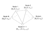
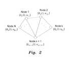
- FIG. 2 diagrammatically illustrates an adaptive network having N nodes.
- boldface letters are used to represent vectors and matrices and non-bolded letters represent scalar quantities.
- Matrices are represented by capital letters and lower-case letters are used to represent vectors.
- the notation (.) T stands for transposition for vectors and matrices, and expectation operations are denoted as E[.].
- FIG. 2 illustrates an exemplary adaptive network having N nodes, where the network has a predefined topology. For each node k, the number of neighbors is given by N k , including the node k itself, as shown in FIG. 2 .
- the output and regressor data are used to produce an estimate of the unknown vector, given by ⁇ k,i .
- the adaptation can be performed using two different techniques.
- the first technique is the Incremental Least Mean Squares (ILMS) method, in which each node updates its own estimate at every iteration and then passes on its estimate to the next node. The estimate of the last node is taken as the final estimate of that iteration.
- the second technique is the Diffusion LMS (DLMS), where each node combines its own estimate with the estimates of its neighbors using some combination technique, and then the combined estimate is used for updating the node estimate.
- This method is referred to as Combine-then-Adapt (CTA) diffusion.
- CTA Combine-then-Adapt
- ATC Adapt-then-Combine
- the conventional Diffusion Lease Mean Square (LMS) technique uses a fixed step-size, which is chosen as a trade-off between steady-state misadjustment and speed of convergence. A fast convergence, as well as low steady-state misadjustment, cannot be achieved with this technique.
- LMS Diffusion Lease Mean Square
- variable step-size least mean square method for estimation in adaptive networks uses a variable step-size to provide estimation for each node in the adaptive network, where the step-size at each node is determined by the error calculated for each node. This is in contrast to conventional least mean square algorithms used in adaptive filters and the like, in which the choice of step-size reflects a tradeoff between misadjustment and the speed of adaptation.
- ⁇ k ⁇ ( i ) ⁇ ⁇ ⁇ ⁇ k ⁇ ( i - 1 ) + ⁇ ⁇ ⁇ l ⁇ N k ⁇ b lk ⁇ e l 2 ⁇ ( i ) , where ⁇ and ⁇ are unitless, selectable parameters, l is an integer, and b lk is a combiner weight for sensed data shared by neighbor nodes of node k; (f) calculating a local estimate for each node neighboring node k, f k,i , for each node k as
- f k , i y k , i - 1 + ⁇ k ⁇ ( i ) ⁇ ⁇ l ⁇ N k ⁇ b lk ⁇ u l T ⁇ ( i ) ⁇ e l ⁇ ( i ) ; (g) calculating the estimate of the output vector y k,i for each node k as
- ⁇ k ⁇ ( i ) ⁇ l ⁇ N k ⁇ c lk ⁇ e l ⁇ ( i ) , where l is an integer, c lk is a combiner coefficient equal to
- ⁇ k ⁇ ( i ) ⁇ ⁇ ⁇ ⁇ k ⁇ ( i - 1 ) + ⁇ ⁇ ⁇ l ⁇ N k ⁇ b lk ⁇ ⁇ l 2 ⁇ ( i ) , where ⁇ and ⁇ are unitless, selectable parameters and b lk is a combiner weight for sensed data shared by neighbor nodes of node k; (g) calculating a local estimate for each node neighboring node k, f k,i , for each node k as
- f k , i y k , i - 1 + ⁇ k ⁇ ( i ) ⁇ ⁇ l ⁇ N k ⁇ b lk ⁇ u l T ⁇ ( i ) ⁇ e l ⁇ ( i ) ; (h) calculating the estimate of the output vector y k,i for each node k as
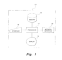
- FIG. 1 is a block diagram of a system for implementing a variable step-size least mean square method for estimation in adaptive networks according to the present invention.
- FIG. 2 is a diagram schematically illustrating an adaptive network with N nodes.
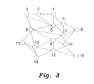
- FIG. 3 is a diagram schematically illustrating network topology for an exemplary simulation of the variable step-size least mean square method for estimation in adaptive networks according to the present invention.
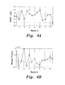
- FIG. 4A is a graph of signal-to-noise ratio as chosen for simulation at each node in the exemplary simulation of FIG. 3 .
- FIG. 4B is a graph of simulated values of noise power at each node in the exemplary simulation of FIG. 3 .
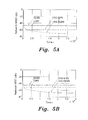
- FIGS. 5A and 5B are comparison plots illustrating mean square deviation as a function of time for two exemplary scenarios using the variable step-size least mean square method for estimation in adaptive networks according to the present invention.
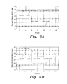
- FIGS. 6A and 6B are comparison plots illustrating steady-state mean square deviations at each node for the exemplary scenarios of FIGS. 5A and 5B , respectively.
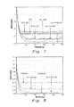
- FIG. 7 is a comparison plot of mean square deviation between alternative embodiments of the present variable step-size least mean square method for estimation in adaptive networks according to the present invention, shown with a signal-to-noise ratio of 0 dB.
- FIG. 8 is a comparison plot of step-size variation vs. iteration number between alternative embodiments of the present variable step-size least mean square method for estimation in adaptive networks according to the present invention, shown with a signal-to-noise ratio of 0 dB.
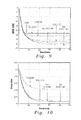
- FIG. 9 is a comparison plot of mean square deviation between alternative embodiments of the present variable step-size least mean square method for estimation in adaptive networks according to the present invention, shown with a signal-to-noise ratio of 10 dB.
- FIG. 10 is a comparison plot of step-size variation vs. iteration number between alternative embodiments of the present variable step-size least mean square method for estimation in adaptive networks according to the present invention, shown with a signal-to-noise ratio of 10 dB.
- variable step-size least mean square method for estimation in adaptive networks uses a variable step-size to provide estimation for each node in the adaptive network, where the step-size at each node is determined by the error calculated for each node.
- This is in contrast to conventional least mean square algorithms used in adaptive filters and the like, in which the choice of step-size reflects a tradeoff between misadjustment and the speed of adaptation.
- An example of a conventional LMS algorithm is shown in chapter ten of A. H. Sayed, Adaptive Filters , New York: Wiley, 2008, pgs. 163-166.
- An example of a variable step-size LMS algorithm is shown in R. H. Kwong and E. W. Johnston, “A Variable Step Size LMS Algorithm”, IEEE Transactions on Signal Processing , Vol. 40, No 7, July 1992, each of which is herein incorporated by reference in its entirety.
- a second, diffusion variable step-size least mean square method of estimation is used.
- Equations (9) and (10) show how the variance of the Gaussian normalized error vector y k iterates from node to node.
- ⁇ _ k ⁇ ⁇ ( M k + ⁇ v , k 2 ) 1 - ⁇ ( 14 )
- ⁇ _ k 2 2 ⁇ ⁇ ⁇ ⁇ _ ⁇ ( ⁇ v , k 2 + M k ) + 3 ⁇ ⁇ 2 ⁇ ( ⁇ v , k 2 + M k ) 2 1 - ⁇ 2 ( 15 )
- M is the steady-state misadjustment for the step-size, given by:
- M k 1 - [ 1 - 2 ⁇ ( 3 - ⁇ ) ⁇ ⁇ v , k 2 1 - ⁇ 2 ⁇ Tr ⁇ ( L ) ] 1 + [ 1 - 2 ⁇ ( 3 - ⁇ ) ⁇ ⁇ v , k 2 1 - ⁇ 2 ⁇ Tr ⁇ ( L ) ] . ( 16 )
- step-size matrix is block-diagonal, the above operations are relatively straightforward.
- Steady-state matrices may be formed for the step-sizes using equations (14) and (15). Using these matrices directly in the steady-state equations provides the MSD and EMSE values for the variable step-size diffusion least mean square method.
- FIG. 5A illustrates the results obtained for the first scenario.
- FIG. 5A there is a great improvement in performance obtained through the usage of both incremental and diffusion variable step-size LMS methods.
- the performance of the variable step-size diffusion LMS method deteriorates only by approximately 3 dB, whereas that of the variable step-size incremental LMS method deteriorates by nearly 9 dB, as shown in FIG. 5B .
- FIGS. 6A and 6B illustrate the steady-state MSD values at each node for both the incremental and diffusion methods, with the variable step-size diffusion LMS method being shown to be superior to both the incremental method and the fixed step-size conventional LMS method.
- FIG. 1 illustrates a generalized system 10 for implementing the variable step-size least mean square method for estimation in adaptive networks, although it should be understood that the generalized system 10 may represent a stand-alone computer, computer terminal, portable computing device, networked computer or computer terminal, or networked portable device.
- Data may be entered into the system 10 by the user via any suitable type of user interface 18 , and may be stored in computer readable memory 14 , which may be any suitable type of computer readable and programmable memory.
- Calculations are performed by the processor 12 , which may be any suitable type of computer processor, and may be displayed to the user on the display 16 , which may be any suitable type of computer display.
- the system 10 preferably includes a network interface 20 , such as a modem or the like, allowing the computer to be networked with either a local area network or a wide area network.
- the processor 12 may be associated with, or incorporated into, any suitable type of computing device, for example, a personal computer or a programmable logic controller.
- the display 16 , the processor 12 , the memory 14 , the user interface 18 , network interface 20 and any associated computer readable media are in communication with one another by any suitable type of data bus, as is well known in the art. Additionally, other standard components, such as a printer or the like, may interface with system 10 via any suitable type of interface.
- Examples of computer readable media include a magnetic recording apparatus, an optical disk, a magneto-optical disk, and/or a semiconductor memory (for example, RAM, ROM, etc.).
- Examples of magnetic recording apparatus that may be used in addition to memory 14 , or in place of memory 14 include a hard disk device (HDD), a flexible disk (ED), and a magnetic tape (MT).
- Examples of the optical disk include a DVD (Digital Versatile Disc), a DVD-RAM, a CD-ROM (Compact Disc-Read Only Memory), and a CD-R (Recordable)/RW.
- equation set (8) An alternative expression for equation set (8) may be given as:
- the Metropolis combiner rule is used, such that:
- c lk ⁇ 1 max ⁇ ( ?? k , ?? l ) , nodes ⁇ ⁇ k ⁇ ⁇ and ⁇ ⁇ l ⁇ ⁇ are ⁇ ⁇ linked ⁇ ⁇ and ⁇ ⁇ k ⁇ l 0 , nodes ⁇ ⁇ k ⁇ ⁇ and ⁇ ⁇ l ⁇ ⁇ are ⁇ ⁇ not ⁇ ⁇ linked 1 - ⁇ l ⁇ ??
- equation (23) may be modified as:
- y k ⁇ ( i + 1 ) w k ⁇ ( i ) + ⁇ k ⁇ ( i ) ⁇ ⁇ l ⁇ N k ⁇ b lk ⁇ u l T ⁇ ( i ) ⁇ e l ⁇ ( i ) , ( 27 )
- b lk is the combiner weight for the sensed data shared by neighbor nodes of node k.
- ⁇ k ⁇ ( i + 1 ) ⁇ k ⁇ ( i ) + ⁇ ⁇ ⁇ l ⁇ N k ⁇ b lk ⁇ e l 2 ⁇ ( i ) , ( 28 ) where ⁇ and ⁇ are the controlling parameters.
- Equation (28) uses the instantaneous error energy to vary the step-size. If the instantaneous errors from neighbor nodes are also shared along with the intermediate update vectors, then equation (28) is modified with:
- ⁇ k ⁇ ( i + 1 ) ⁇ k ⁇ ( i ) + ⁇ ⁇ ⁇ l ⁇ N k ⁇ b lk ⁇ ⁇ l 2 ⁇ ( i ) . ( 30 )
- Equation (27), (28), (29) and (30) represents the Generalized NVSSDLMS method.
- the VSSDLMS method has one extra update equation for the step-size, which includes three multiplications and one addition per node more than the DLMS method.
- the generalized VSSDLMS method there are 2MN k extra multiplications and M(N k ⁇ 1) extra additions in equation (27), and 2N k +3 extra multiplications and N k extra additions in equation (28).
- the generalized VSSDLMS algorithm has a total of 2(M+1)N k +3 extra multiplications and (M+1)N k ⁇ M extra additions per node.
- the NVSSDLMS algorithm has a further N k extra multiplications and N k ⁇ 1 extra additions per node and the same number of extra computations per node for the generalized NVSSDLMS method.
- VSSDLMS 3 1 Gen VSSDLMS 2(M + 1)N k + 3 (M + 1)N k ⁇ M NVSSDLMS N k + 3 N k Gen NVSSDLMS (2M + 3)N k + 3 (M + 2)N k ⁇ M ⁇ 1
- FIGS. 7-10 the performance of the NVSSDLMS method is compared with the DLMS method and the VSSDLMS method.
- a network of twenty nodes is used.
- Results are shown for signal-to-noise ratio (SNR) values of 0 dB ( FIGS. 7 and 8 ) and 10 dB ( FIGS. 9 and 10 ).
- SNR signal-to-noise ratio
- FIGS. 7 and 8 show the results for a SNR of 0 dB
- FIGS. 9 and 10 show the results for a SNR of 10 dB.
- the VSSDLMS method does not perform well at an SNR of 0 dB.
- the NVSSDLMS method performs quite well.
- the generalized VSSDLMS algorithm also performs better than the generalized DLMS case, but the generalized NVSSDLMS method outperforms the generalized VSSDLMS method.
- FIG. 8 illustrates how the step-size varies.
- the step-size variation is best for the NVSSDLMS method, as it becomes slightly less than that of the generalized NVSSDLMS method. However, the overall performance of the generalized NVSSDLMS method is better.
- FIG. 9 shows that the VSSDLMS methods perform better than the DLMS methods, but the NVSSDLMS methods outperform both the VSSDLMS methods.
- FIG. 10 shows the step-size variation for this case. As can be seen from FIG. 10 , the step-size performance for all methods is similar to mean square deviation (MSD) performance.
- MSD mean square deviation
Landscapes
- Engineering & Computer Science (AREA)
- Physics & Mathematics (AREA)
- Mathematical Physics (AREA)
- Theoretical Computer Science (AREA)
- Data Mining & Analysis (AREA)
- General Physics & Mathematics (AREA)
- Pure & Applied Mathematics (AREA)
- Mathematical Optimization (AREA)
- Algebra (AREA)
- Computational Mathematics (AREA)
- Databases & Information Systems (AREA)
- Software Systems (AREA)
- General Engineering & Computer Science (AREA)
- Mathematical Analysis (AREA)
- Computer Networks & Wireless Communication (AREA)
- Signal Processing (AREA)
- Data Exchanges In Wide-Area Networks (AREA)
Abstract
Description
d k(i)=u k,i +w 0 +v k(i), (1)
where uk,i, is a known regressor row vector of length M, w0 is an unknown column vector of length M, and vk(i) represents noise. The output and regressor data are used to produce an estimate of the unknown vector, given by ψk,i.
where {clk}1εN
where l is an integer, clk represents a combination weight for node k, which is fixed; (h) if ek(i) is greater than a selected error threshold, then setting i=i+1 and returning to step (c); otherwise, (i) defining a set of output vectors yk for each node k, where yk=yk,i; and (j) storing the set of output vectors in computer readable memory.
where α and γ are unitless, selectable parameters, l is an integer, and blk is a combiner weight for sensed data shared by neighbor nodes of node k; (f) calculating a local estimate for each node neighboring node k, fk,i, for each node k as
(g) calculating the estimate of the output vector yk,i for each node k as
where clk is a combiner coefficient equal to
when nodes k and l are linked and k does not equal l, clk is equal to 0 when nodes k and l are not linked, and clk is equal to
when k equals l; (h) if ek(i) is greater than a selected error threshold, then setting i=i+1 and returning to step (c); otherwise, (i) defining a set of output vectors yk for each node k, where yk=yk,i; and (j) storing the set of output vectors in computer readable memory.
where l is an integer, clk is a combiner coefficient equal to
when nodes k and l are linked and k does not equal l, clk, is equal to 0 when nodes k and l are not linked, and clk is equal to
when k equals l, (f) calculating a node step size μk for each node k as
where α and γ are unitless, selectable parameters and blk is a combiner weight for sensed data shared by neighbor nodes of node k; (g) calculating a local estimate for each node neighboring node k, fk,i, for each node k as
(h) calculating the estimate of the output vector yk,i for each node k as
(i) if ek(i) is greater than a selected error threshold, then setting i=i+1 and returning to step (c); otherwise, (j) defining a set of output vectors yk for each node k, where yk=yk,i; and (k) storing the set of output vectors in computer readable memory.
y k,i =y k-1,i+μk(i)u k,i T(d k(i)−u k,i y k-1,i). (3)
Every node updates its estimate based on the updated estimate coming from the previous node. The error is given by:
e k(i)=d k(i)−u k,i y k-1,i. (4)
The node step size μk is given by:
μk(i)=αμk(i−1)+γe 2(i) (5)
where α and γ are controlling parameters. Updating equation (3) with the step-size given by equation (5) results in the variable step-size incremental least mean square method defined by the following recursion:
y k,i =y k-1,i+μk(i)u k,i T(d k(i)−u k,i y k-1,i). (6)
e k(i)=d k(i)−u k,i y k,i-1. (7)
Applying this error to equation (5) yields the following update equations:
where l is an integer, clk represents a combination weight for node k, which is fixed; (h) if ek(i) is greater than a selected error threshold, then setting i=i+1 and returning to step (c); otherwise, (i) defining a set of output vectors yk for each node k, where yk=yk,i; and (j) storing the set of output vectors in computer readable memory.
E└∥
where
E└μ k(i)u k,i T e k(i)┘=E[μ k(i)]E└u k,i T e k(i)┘, (11)
thus yielding the following new recursions, respectively, from equations (9) and (10):
where M is the steady-state misadjustment for the step-size, given by:
where
b=bvec{R v D 2 L} (20)
where Rv is the noise auto-correlation matrix, bvec{.} is the block vectorization operator, D is the block diagonal step-size matrix for the whole network,
b=bvec{R v E└D 2 ┘L}. (22)
where yk(i) is the intermediate local estimate at node k at time instant i, μk is the step size associated with the kth node, and clk, represents the combiner coefficient. Various choices for combiner coefficients are possible. In the present method, the Metropolis combiner rule is used, such that:
where the error at the node is given by the equivalent of equation (7):
e k(i)=d k(i)−u k,i y k,i-1. (26)
where blk is the combiner weight for the sensed data shared by neighbor nodes of node k.
where α and γ are the controlling parameters.
where εk(i) is the diffused error for node k. Thus, equation (28) becomes:
| TABLE 1 |
| Complexity Comparisons Per Node |
| Algorithm | Extra Multiplications | | ||
| VSSDLMS | ||||
| 3 | 1 | |||
| Gen VSSDLMS | 2(M + 1)Nk + 3 | (M + 1)Nk − M | ||
| NVSSDLMS | Nk + 3 | Nk | ||
| Gen NVSSDLMS | (2M + 3)Nk + 3 | (M + 2)Nk − M − 1 | ||
Claims (1)
Priority Applications (1)
| Application Number | Priority Date | Filing Date | Title |
|---|---|---|---|
| US13/286,172 US8903685B2 (en) | 2010-10-27 | 2011-10-31 | Variable step-size least mean square method for estimation in adaptive networks |
Applications Claiming Priority (2)
| Application Number | Priority Date | Filing Date | Title |
|---|---|---|---|
| US12/913,482 US8547854B2 (en) | 2010-10-27 | 2010-10-27 | Variable step-size least mean square method for estimation in adaptive networks |
| US13/286,172 US8903685B2 (en) | 2010-10-27 | 2011-10-31 | Variable step-size least mean square method for estimation in adaptive networks |
Related Parent Applications (1)
| Application Number | Title | Priority Date | Filing Date |
|---|---|---|---|
| US12/913,482 Continuation-In-Part US8547854B2 (en) | 2010-10-27 | 2010-10-27 | Variable step-size least mean square method for estimation in adaptive networks |
Publications (2)
| Publication Number | Publication Date |
|---|---|
| US20120109600A1 US20120109600A1 (en) | 2012-05-03 |
| US8903685B2 true US8903685B2 (en) | 2014-12-02 |
Family
ID=45997624
Family Applications (1)
| Application Number | Title | Priority Date | Filing Date |
|---|---|---|---|
| US13/286,172 Expired - Fee Related US8903685B2 (en) | 2010-10-27 | 2011-10-31 | Variable step-size least mean square method for estimation in adaptive networks |
Country Status (1)
| Country | Link |
|---|---|
| US (1) | US8903685B2 (en) |
Cited By (1)
| Publication number | Priority date | Publication date | Assignee | Title |
|---|---|---|---|---|
| US11308349B1 (en) | 2021-10-15 | 2022-04-19 | King Abdulaziz University | Method to modify adaptive filter weights in a decentralized wireless sensor network |
Families Citing this family (13)
| Publication number | Priority date | Publication date | Assignee | Title |
|---|---|---|---|---|
| EP2465050A4 (en) * | 2009-09-03 | 2014-01-29 | Wallace E Larimore | METHOD AND SYSTEM FOR EMPIRICAL MODELING OF TIME-VARYING SYSTEMS WITH VARIABLE AND NON-LINEAR PARAMETERS USING LINEAR VARIETY ITERATIVE CALCULATIONS |
| US8547854B2 (en) * | 2010-10-27 | 2013-10-01 | King Fahd University Of Petroleum And Minerals | Variable step-size least mean square method for estimation in adaptive networks |
| US9385917B1 (en) | 2011-03-31 | 2016-07-05 | Amazon Technologies, Inc. | Monitoring and detecting causes of failures of network paths |
| US9104543B1 (en) * | 2012-04-06 | 2015-08-11 | Amazon Technologies, Inc. | Determining locations of network failures |
| US8937870B1 (en) | 2012-09-11 | 2015-01-20 | Amazon Technologies, Inc. | Network link monitoring and testing |
| US9197495B1 (en) | 2013-02-11 | 2015-11-24 | Amazon Technologies, Inc. | Determining locations of network failures |
| US9210038B1 (en) | 2013-02-11 | 2015-12-08 | Amazon Technologies, Inc. | Determining locations of network failures |
| US9742638B1 (en) | 2013-08-05 | 2017-08-22 | Amazon Technologies, Inc. | Determining impact of network failures |
| US9654904B2 (en) * | 2015-02-19 | 2017-05-16 | Xerox Corporation | System and method for flexibly pairing devices using adaptive variable thresholding |
| CN106209930A (en) * | 2015-04-30 | 2016-12-07 | 神盾股份有限公司 | Sensor network system, its method and nodes |
| US10310518B2 (en) * | 2015-09-09 | 2019-06-04 | Apium Inc. | Swarm autopilot |
| CN110190832B (en) * | 2019-06-09 | 2023-02-24 | 苏州大学 | Multi-task Adaptive Filter Networks with Variable Regularization Parameters |
| CN119865509B (en) * | 2023-10-20 | 2026-04-17 | 小米科技(武汉)有限公司 | Electrical signal parameter estimation method, electrical signal parameter estimation device, electronic equipment and storage medium |
Citations (18)
| Publication number | Priority date | Publication date | Assignee | Title |
|---|---|---|---|---|
| US5546459A (en) | 1993-11-01 | 1996-08-13 | Qualcomm Incorporated | Variable block size adaptation algorithm for noise-robust acoustic echo cancellation |
| US5887059A (en) | 1996-01-30 | 1999-03-23 | Advanced Micro Devices, Inc. | System and method for performing echo cancellation in a communications network employing a mixed mode LMS adaptive balance filter |
| US6026121A (en) | 1997-07-25 | 2000-02-15 | At&T Corp | Adaptive per-survivor processor |
| EP1054536A2 (en) | 1999-05-20 | 2000-11-22 | Nec Corporation | Non-recursive adaptive filter, with variable orders of non-linear processing |
| US20020041678A1 (en) | 2000-08-18 | 2002-04-11 | Filiz Basburg-Ertem | Method and apparatus for integrated echo cancellation and noise reduction for fixed subscriber terminals |
| US6377611B1 (en) | 1999-02-01 | 2002-04-23 | Industrial Technology Research Institute | Apparatus and method for a DSSS/CDMA receiver |
| US6493689B2 (en) * | 2000-12-29 | 2002-12-10 | General Dynamics Advanced Technology Systems, Inc. | Neural net controller for noise and vibration reduction |
| US20040044712A1 (en) | 1998-12-31 | 2004-03-04 | Staszewski Robert B. | Method and architecture for controlling asymmetry of an LMS adaptation algorithm that controls FIR filter coefficients |
| US6741707B2 (en) | 2001-06-22 | 2004-05-25 | Trustees Of Dartmouth College | Method for tuning an adaptive leaky LMS filter |
| KR20050001888A (en) | 2003-06-26 | 2005-01-07 | 백종섭 | Method and Device for Channel Equalization |
| US20050027494A1 (en) * | 2003-03-31 | 2005-02-03 | University Of Florida | Accurate linear parameter estimation with noisy inputs |
| US20050201457A1 (en) | 2004-03-10 | 2005-09-15 | Allred Daniel J. | Distributed arithmetic adaptive filter and method |
| US6977912B1 (en) | 1999-06-11 | 2005-12-20 | Axxcelera Broadband Wireless | Control signalling and dynamic channel allocation in a wireless network |
| US7298774B2 (en) | 2000-08-25 | 2007-11-20 | Sanyo Electric Co., Ltd. | Adaptive array device, adaptive array method and program |
| US20080136645A1 (en) | 2006-12-12 | 2008-06-12 | Industrial Technology Research Institute | Rfid reader and circuit and method for echo cancellation thereof |
| CN101222458A (en) | 2008-01-22 | 2008-07-16 | 上海师范大学 | Low-Order Recursive Minimum Mean Square Error Estimation for MIMO-OFDM Channels |
| CN101252559A (en) | 2007-10-12 | 2008-08-27 | 电子科技大学中山学院 | Training sequence time-varying step length least mean square method |
| US20080260141A1 (en) | 2007-04-18 | 2008-10-23 | Gas Technology Institute | Method and apparatus for enhanced convergence of the normalized LMS algorithm |
-
2011
- 2011-10-31 US US13/286,172 patent/US8903685B2/en not_active Expired - Fee Related
Patent Citations (18)
| Publication number | Priority date | Publication date | Assignee | Title |
|---|---|---|---|---|
| US5546459A (en) | 1993-11-01 | 1996-08-13 | Qualcomm Incorporated | Variable block size adaptation algorithm for noise-robust acoustic echo cancellation |
| US5887059A (en) | 1996-01-30 | 1999-03-23 | Advanced Micro Devices, Inc. | System and method for performing echo cancellation in a communications network employing a mixed mode LMS adaptive balance filter |
| US6026121A (en) | 1997-07-25 | 2000-02-15 | At&T Corp | Adaptive per-survivor processor |
| US20040044712A1 (en) | 1998-12-31 | 2004-03-04 | Staszewski Robert B. | Method and architecture for controlling asymmetry of an LMS adaptation algorithm that controls FIR filter coefficients |
| US6377611B1 (en) | 1999-02-01 | 2002-04-23 | Industrial Technology Research Institute | Apparatus and method for a DSSS/CDMA receiver |
| EP1054536A2 (en) | 1999-05-20 | 2000-11-22 | Nec Corporation | Non-recursive adaptive filter, with variable orders of non-linear processing |
| US6977912B1 (en) | 1999-06-11 | 2005-12-20 | Axxcelera Broadband Wireless | Control signalling and dynamic channel allocation in a wireless network |
| US20020041678A1 (en) | 2000-08-18 | 2002-04-11 | Filiz Basburg-Ertem | Method and apparatus for integrated echo cancellation and noise reduction for fixed subscriber terminals |
| US7298774B2 (en) | 2000-08-25 | 2007-11-20 | Sanyo Electric Co., Ltd. | Adaptive array device, adaptive array method and program |
| US6493689B2 (en) * | 2000-12-29 | 2002-12-10 | General Dynamics Advanced Technology Systems, Inc. | Neural net controller for noise and vibration reduction |
| US6741707B2 (en) | 2001-06-22 | 2004-05-25 | Trustees Of Dartmouth College | Method for tuning an adaptive leaky LMS filter |
| US20050027494A1 (en) * | 2003-03-31 | 2005-02-03 | University Of Florida | Accurate linear parameter estimation with noisy inputs |
| KR20050001888A (en) | 2003-06-26 | 2005-01-07 | 백종섭 | Method and Device for Channel Equalization |
| US20050201457A1 (en) | 2004-03-10 | 2005-09-15 | Allred Daniel J. | Distributed arithmetic adaptive filter and method |
| US20080136645A1 (en) | 2006-12-12 | 2008-06-12 | Industrial Technology Research Institute | Rfid reader and circuit and method for echo cancellation thereof |
| US20080260141A1 (en) | 2007-04-18 | 2008-10-23 | Gas Technology Institute | Method and apparatus for enhanced convergence of the normalized LMS algorithm |
| CN101252559A (en) | 2007-10-12 | 2008-08-27 | 电子科技大学中山学院 | Training sequence time-varying step length least mean square method |
| CN101222458A (en) | 2008-01-22 | 2008-07-16 | 上海师范大学 | Low-Order Recursive Minimum Mean Square Error Estimation for MIMO-OFDM Channels |
Non-Patent Citations (9)
| Title |
|---|
| Amir Rastegarnia, Mohammad Ali Tinati and Azam Khalili, A Diffusion Least-Mean Square Algorithm for Distributed Estimation over Sensor Networks, World Academy of Science, Engineering and Technology vol. 2 Sep. 26, 2008, 5 pages. * |
| Bin Saeed, M.O.; Zerguine, A.; Zummo S.A., "Noise Constrained Diffusion Least Mean Squares Over Adaptive Networks", 2010 IEEE 21st International Symposium on Personal Indoor and Mobile Radio Communications, Sep. 26-30, 2010, pp. 282-292. |
| Cattivelli, F.; Sayed, A.H., "Diffusion LMS Strategies for Distributed Estimation", IEEE Transactions on Signal Processing, vol. 58, No, 3, Mar. 2010, 14 pages. |
| Cattivelli, F.; Sayed, A.H., "Diffusion LMS-Based Distributed Detection over Adaptive Networks", Signals, Systems and Computers, 2009 Conference Record of the Forty-Third Asilomar Conference on, Nov. 1-4, 2009, pp. 171-175. |
| Lopes, C.G.; Sayed, A.H., "Incremental Adaptive Strategies Over Distributed Networks", IEEE Transactions on Signal Processing, vol. 55, No. 8, Aug. 2007. |
| M.O. Bin Saeed, A. Zerguine and S.A. Zummo, "Variable Step-Size Least Mean Square Algorithms Over Adaptive Networks", 10th International Conference on Information Science, Signal Processing and their Applications (ISSPA 2010), May 2010, pp. 381-384. |
| M.S.E. Abadi, S.Z. Moussavi and A.M. Far, "Variable, Step-Size, Block Normalized, Least Mean, Square Adaptive Filter: A Unified Framework", Scientia Iranica, vol. 15, No. 2, pp. 195-202, Apr. 2008. |
| R.H. Kwong and E.W. Johnston, "A Variable Step Size LMS Algorithm", IEEE Transactions on Signal Processing, vol. 40, No. 7, Jul. 1992, 10 pages. |
| W.Y. Chen and R.A. Haddad, "A Variable Step Size LMS Algorithm", Circuits and Systems,1990, Proceedings of the 33rd Midwest Symposium on, Aug. 12-14, 1990, vol. 1, pp. 423-426. |
Cited By (1)
| Publication number | Priority date | Publication date | Assignee | Title |
|---|---|---|---|---|
| US11308349B1 (en) | 2021-10-15 | 2022-04-19 | King Abdulaziz University | Method to modify adaptive filter weights in a decentralized wireless sensor network |
Also Published As
| Publication number | Publication date |
|---|---|
| US20120109600A1 (en) | 2012-05-03 |
Similar Documents
| Publication | Publication Date | Title |
|---|---|---|
| US8903685B2 (en) | Variable step-size least mean square method for estimation in adaptive networks | |
| US8547854B2 (en) | Variable step-size least mean square method for estimation in adaptive networks | |
| US8462892B2 (en) | Noise-constrained diffusion least mean square method for estimation in adaptive networks | |
| KR20060018882A (en) | A method for providing link reliability measures to routing protocols in ad hoc wireless networks | |
| Chouvardas et al. | Trading off complexity with communication costs in distributed adaptive learning via Krylov subspaces for dimensionality reduction | |
| CN101305526B (en) | Reducing power estimated complex degree | |
| Li et al. | Distributed adaptive estimation based on the APA algorithm over diffusion networks with changing topology | |
| CN117099055A (en) | Methods, apparatus and systems for configuring communication links used to exchange data related to cooperative control algorithms | |
| US20130110478A1 (en) | Apparatus and method for blind block recursive estimation in adaptive networks | |
| Abdolee et al. | Tracking performance and optimal adaptation step-sizes of diffusion-LMS networks | |
| Aduroja et al. | Distributed principal components analysis in sensor networks | |
| Saeed et al. | Variable step-size least mean square algorithms over adaptive networks | |
| Jamali-Rad et al. | Dynamic multidimensional scaling for low-complexity mobile network tracking | |
| US20030231599A1 (en) | Optimum route calculation method and storage medium which stores optimum route calculation program | |
| Imanian et al. | Information-Based Node Selection for Joint PCA and Compressive Sensing-Based Data Aggregation | |
| JP7397956B1 (en) | Power control method and its communication device | |
| CN116170256B (en) | Active user detection and channel estimation method and device | |
| Zhao et al. | Combination weights for diffusion strategies with imperfect information exchange | |
| CN106341356A (en) | Downlink carrier flatness compensation method and device | |
| Levendovszky et al. | Adaptive statistical algorithms in network reliability analysis | |
| Mateos et al. | Consensus-based distributed least-mean square algorithm using wireless ad hoc networks | |
| Kim et al. | Joint power adaptation, scheduling and routing framework for wireless ad-hoc networks | |
| CN107147995B (en) | Wireless location method based on Tikhonov regularization | |
| US9699707B2 (en) | Calculation methods and calculation devices | |
| Basnarkov et al. | Biased random search in complex networks |
Legal Events
| Date | Code | Title | Description |
|---|---|---|---|
| AS | Assignment |
Owner name: KING FAHD UNIVERSITY OF PETROLEUM AND MINERALS, SA Free format text: ASSIGNMENT OF ASSIGNORS INTEREST;ASSIGNORS:SAEED, MUHAMMAD OMER BIN, MR.;ZERGUINE, AZZEDINE, DR.;REEL/FRAME:027151/0280 Effective date: 20111025 |
|
| STCF | Information on status: patent grant |
Free format text: PATENTED CASE |
|
| MAFP | Maintenance fee payment |
Free format text: PAYMENT OF MAINTENANCE FEE, 4TH YR, SMALL ENTITY (ORIGINAL EVENT CODE: M2551) Year of fee payment: 4 |
|
| FEPP | Fee payment procedure |
Free format text: MAINTENANCE FEE REMINDER MAILED (ORIGINAL EVENT CODE: REM.); ENTITY STATUS OF PATENT OWNER: SMALL ENTITY |
|
| LAPS | Lapse for failure to pay maintenance fees |
Free format text: PATENT EXPIRED FOR FAILURE TO PAY MAINTENANCE FEES (ORIGINAL EVENT CODE: EXP.); ENTITY STATUS OF PATENT OWNER: SMALL ENTITY |
|
| STCH | Information on status: patent discontinuation |
Free format text: PATENT EXPIRED DUE TO NONPAYMENT OF MAINTENANCE FEES UNDER 37 CFR 1.362 |
|
| FP | Lapsed due to failure to pay maintenance fee |
Effective date: 20221202 |