US8886497B1 - Computer simulation of electromagnetic fields - Google Patents
Computer simulation of electromagnetic fields Download PDFInfo
- Publication number
- US8886497B1 US8886497B1 US13/136,010 US201113136010A US8886497B1 US 8886497 B1 US8886497 B1 US 8886497B1 US 201113136010 A US201113136010 A US 201113136010A US 8886497 B1 US8886497 B1 US 8886497B1
- Authority
- US
- United States
- Prior art keywords
- boundary
- potential
- basis function
- basis
- right arrow
- Prior art date
- Legal status (The legal status is an assumption and is not a legal conclusion. Google has not performed a legal analysis and makes no representation as to the accuracy of the status listed.)
- Expired - Fee Related, expires
Links
Images


Classifications
-
- G—PHYSICS
- G06—COMPUTING OR CALCULATING; COUNTING
- G06F—ELECTRIC DIGITAL DATA PROCESSING
- G06F17/00—Digital computing or data processing equipment or methods, specially adapted for specific functions
- G06F17/10—Complex mathematical operations
- G06F17/11—Complex mathematical operations for solving equations, e.g. nonlinear equations, general mathematical optimization problems
- G06F17/13—Differential equations
-
- G—PHYSICS
- G06—COMPUTING OR CALCULATING; COUNTING
- G06F—ELECTRIC DIGITAL DATA PROCESSING
- G06F30/00—Computer-aided design [CAD]
- G06F30/20—Design optimisation, verification or simulation
- G06F30/23—Design optimisation, verification or simulation using finite element methods [FEM] or finite difference methods [FDM]
-
- G—PHYSICS
- G06—COMPUTING OR CALCULATING; COUNTING
- G06F—ELECTRIC DIGITAL DATA PROCESSING
- G06F30/00—Computer-aided design [CAD]
- G06F30/30—Circuit design
- G06F30/36—Circuit design at the analogue level
- G06F30/367—Design verification, e.g. using simulation, simulation program with integrated circuit emphasis [SPICE], direct methods or relaxation methods
-
- G—PHYSICS
- G06—COMPUTING OR CALCULATING; COUNTING
- G06F—ELECTRIC DIGITAL DATA PROCESSING
- G06F2111/00—Details relating to CAD techniques
- G06F2111/10—Numerical modelling
Definitions
- FIG. 1 shows a sphere with a nearby physical point dipole, represented as a dot.
- FIG. 2 shows these dipole points, colored black; the dashed lines indicate the associations between dipole points and boundary vertices.
- FIG. 3 shows the sphere, a dipole in the external region, and a plane containing the dipole and the center of the sphere.
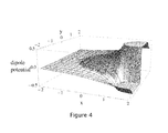
- FIG. 4 is a plot of a scalar potential in the plane identified in the previous figure.
- FIG. 5 is a plot of a discontinuous scalar potential ⁇ i defined in the simulation space made up of the actual mediums inside and outside the sphere.
- FIG. 6 shows the sphere, a dipole in the internal region, and a plane containing the dipole and the center of the sphere.
- FIG. 7 is a plot of the scalar potential in the plane identified in the previous figure.
- FIG. 8 is a plot of a discontinuous scalar potential ⁇ i defined in the simulation space.
- FIG. 9 shows a sphere, the simulation's physical dipole in the external region, a plane containing the dipole, and the center of the sphere.
- FIG. 10 is a plot of the discontinuous scalar potential defined in the simulation space.
- FIG. 11 shows the scalar part of the interior discontinuous potential function that matches this physical dipole at the boundary.
- FIG. 12 shows potentials that is the sum of one interior discontinuous potential and one exterior discontinuous potential.
- FIG. 13 shows a potential that is the sum of the potentials of the FIG. 10 and of FIG. 11
- FIG. 14 shows a triangular mesh
- FIG. 15 shows a representation of a wire network.
- FIG. 16 shows an example of half-basis charge functions.
- FIG. 17 shows an example of a basis charge function.
- FIG. 18 shows an example of the domains of two half-basis functions for a thin dome-shaped sheet.
- FIG. 19 shows the total basis line charge density from three charges.
- FIG. 20 shows the current required to satisfy the continuity equation for the charge density of FIG. 19 .
- FIG. 21 shows a plot of domain (the parts of the wire network where the function is nonzero) of each unmodified basis function.
- FIG. 22 shows a plot of another set of basis functions.
- FIG. 23 shows icosahedron vertexes with one point inside the sphere and one point outside the sphere.
- FIG. 24 shows the graph of FIG. 23 with additional points on the boundary for numerically approximating boundary integrals.
- FIG. 25 shows a plot with frame vectors drawn next to the virtual dipoles.
- FIGS. 26 and 27 show the scalar potential (that is, the zeroth component of the space-time potential) of the first element of AIO.
- FIGS. 28 and 29 show some vector potential values, for check for the continuity of the tangential component at the surface of the sphere.
- FIG. 30 shows plots over a larger range, indicating the increasing imaginary part at larger radii, which is just part of a wave.
- FIG. 33 the vector potential for a virtual electric dipole source.
- FIG. 34 shows frame vectors.
- FIG. 34 is at 45 degrees to the x and y axes.
- FIG. 35 shows the magnetic field, B, in the x-z plane.
- FIG. 36 shows a discontinuity in B at the boundary.
- FIGS. 37 and 38 shows the E field of the ⁇ 1,2 ⁇ basis function.
- FIG. 39 shows a couple of plots of the E field of basis function ⁇ 1,1 ⁇ , representing dipoles associated with vertex 1 and frame vector 1.
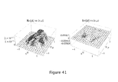
- FIGS. 40 and 41 show a substantially continuous scalar potential associated with the specified external source, a dipole at ⁇ 3, 0, 0 ⁇ of type 2 (magnetic) with moment ⁇ 0,1,0 ⁇ .
- FIGS. 42 and 43 show a vector potential.
- FIG. 44 is a plot of the real and imaginary parts of the electric field.
- FIG. 45 is another plot of a vector potential.
- FIG. 46 shows that the example of FIG. 45 example is for wavelengths that are large, but not very much larger, than the size of the object.
- FIGS. 47 and 48 show the real and imaginary parts of the B field in the ⁇ x,y ⁇ and ⁇ z,y ⁇ planes.
- FIG. 49 shows the Real and Imaginary parts of the electric field E in the xz plane.
- FIG. 50 shows plots in which the magnetic dipole axis is pointed out of the paper (since it is along the y axis).
- a person skilled in the arts relevant to this provisional patent application may be a person a) with good command of electrodynamics at the level of the classic textbooks “Classical Electrodynamics” by Jackson (2nd ed, Wiley, 1975) and “The Classical Theory of Fields” by Landau and Lifshitz (Pergamon Press, 1975), b) skilled at programming in the Mathematica computer language, version 7, in order to easily and clearly understand the numerical implementation example, and c) familiar with the use of geometric algebra and calculus at the level of “Geometric Algebra for Physicists” by Doran and Lasenby (Cambridge University Press, 2003) and preferably also familiar with “Space-Time Algebra” by Hestenes (Gordon and Breach, 1966) in order to clearly understand how the calculations done in the numerical implementation example can be correctly applied to other electromagnetic simulations.
- the first method or claim is to choose the parameters in a parameterized expression of the potential and associated field so as to extremize the electromagnetic action with variation of those parameters. I call this the Method of Least Action.
- This method may be viewed as a boundary element method, or a method of moments, that uses unknowns, operators, weighting functions, and an inner product that are different from those used in prior art.
- This method has improved numerical results for the same computational time compared with prior art, and a simpler, more precisely defined structure which allows easier application and extension to cases that are more complex than the simple case used here for illustration.
- time dependence is harmonic, with arbitrarily varying time-dependent electromagnetic quantities represented as Fourier components in the frequency domain, but this description may be recast in the time domain.
- This method may be especially usefully applied to simulate electromagnetic fields when space may be modeled as consisting substantially of piecewise homogeneous bulk regions of space filled with media that is electrically polarizable, electrically conductive, magnetically polarizable, or some combination.
- Bulk regions means bounded volumes that are not thin; more quantitatively, we might say that bulk regions are bounded volumes such that the ratio of volume to surface area is sufficiently large, typically not much smaller than the distance between points or vertices on the region's boundary used to describe the boundary. Bounded volumes that are not bulk regions may be called thin regions or objects, or regions or objects with negligible thickness, or points or particles, or wires, or sheets.
- a thin surface layer of a bulk region is treated as a separate thin region; for example, in many cases almost all charge and current of a good electrical conductor is very close to the surface of the conducting object, and a bulk volume conductor may be replaced, either or both in physical reality and in the computer simulation, by a thin conducting surface or sheet object that is coincident with the boundary of the original conducting object.
- the space may contain additional material, such as polarizable or conductive point, wire, or sheet or other thin objects; these can be analyzed by combining the method of least action with prior art methods, or, preferably, with the method of least squared response error described below and in later sections.
- additional material such as polarizable or conductive point, wire, or sheet or other thin objects
- a “substantially continuous electromagnetic space-time potential” refers to a scalar potential and 3D vector potential that are continuous at all non-boundary points, and such that the scalar potential and the components of the vector potential that are tangential to the boundary are continuous at all boundary points within an acceptable numerical error.
- the continuous potential requirement of Item a) ensures that the two homogeneous Maxwell equations are satisfied at all non-boundary points, and that the usual homogeneous electromagnetic boundary conditions are satisfied at all boundary points.
- Item i) ensures that the two Inhomogeneous Maxwell equations are satisfied at every non-boundary point.
- Item ii) ensures that the usual Inhomogeneous electromagnetic boundary conditions are satisfied.
- This item results in an equation of the type used by a method of moments or by boundary element methods as applied to electromagnetism in prior art, but with an inner product, weighting functions, equation, and unknowns that have not been used in prior art, and it results in significant improvement in performance and results over prior art. This may be the most important and novel part of my method of least action.
- the same equivalent source is generally used for fields on both sides of a boundary, and it is generally necessary to choose equivalent sources that include nonphysical magnetic charge and current; in the present method, different boundary virtual sources are used for fields on the different sides of a boundary, and using only electric charge and current, not magnetic, is allowed and may be preferred.
- 3) Specify a “virtual” parameterized conserved charge and current source density that is outside the region for which the fields are being calculated, calculate the potential and fields from this virtual charge and current, and then constrain the virtual sources so that the desired boundary conditions are met.
- Such virtual source density is similar to virtual images in optics, in that the virtual object does not really exist but is a convenient fiction for calculating desired field values in a region that is free of the virtual object.
- the charge-current source density is simple, such as consisting of a finite number of point electric and magnetic dipoles, and the sources are well chosen, such as point dipoles at distances from the boundary that are comparable to the distance between dipoles, and the fields are well chosen, such as both retarded and advanced fields, this method can generate a good approximation to a wide range of potential values on boundaries between bulk regions with relatively little computation.
- Using virtual sources allows much greater freedom in choosing good basis functions.
- These virtual sources can be a combination of boundary and non-boundary virtual sources, as may be useful for a region boundary with one part that comes close to but does not directly connect with another part of the boundary (since in this case the non-boundary virtual sources that should be on one side of the boundary may end up on the other side, so boundary virtual sources might be a better choice).
- This new method of including non-boundary virtual sources may be used here and has not been used in prior art, and indeed cannot be used in much if not all prior art since the source is used as the “weighting” or “testing” function for essential integrals over boundaries in prior art.
- Use of virtual sources is illustrated in detail in the computer program in the “Numerical implementation example” section.
- This method of least action can be expressed in detail and with precision in various ways, including using conventional 3D vector algebra, relativistic tensor algebra, the geometric algebra of space, and the geometric algebra of space-time. Despite the simplicity of its statement and its advantages, it has not previously been applied in the art of numerical electromagnetic calculation or computer simulation. Details of this method are given in later sections.
- a second method or claim of this patent is the determination of the coefficients of source basis functions for thin objects or regions, such as thin wires or thin sheets, that are electromagnetically responsive (e.g., electrically conductive or electrically or magnetically polarizable, or some combination) by choosing coefficients that minimize the integrated squared error between the source given by the sum of coefficients times basis functions, and the source predicted by the electromagnetic response rule (e.g., Ohm's “Law”) as a linear function of the field, with the field calculated due to all charge-current sources, typically using integrals and Green's functions.
- the electromagnetic response rule e.g., Ohm's “Law”
- a third method or claim of this patent is the application of a new type of wire-like or sheet-like charge-current source basis function set.
- This type of set of source basis functions can be obtained from a more conventional set of more localized conserved charge-current source basis functions, such as RWO basis functions, as follows. We begin by choosing to parameterize each basis function by the amplitude of the charge density. We then replace one charge-current source basis function in each topological loop of the wire or sheet network with a linear combination of the original basis functions of the loop so that they represent a current loop, with coefficients chosen so that the charge density is zero everywhere, and then divide the resulting function by the frequency.
- the resulting set of source basis functions works without problem at all frequencies (with the usual restriction that the domain of the basis function is small compared with the wavelength of radiation in the surrounding medium), including low frequencies and zero.
- the original set of source basis functions is problematic at low frequencies because the linear combination of basis functions described above has a common factor of frequency, so this combination vanishes at zero frequency, resulting in complete loss of this degree of freedom for zero frequency (with a corresponding completely incorrect solution to the simulation problem) and serious numerical problems for small frequencies.
- This may be used in combination with the method of least action, the method of least squared response error, or prior art methods. Further details are give in a “Description of Wires and Sheets” section.
- a fourth method or claim of this patent is the use of both retarded and advanced potential and field functions as basis functions in computer simulations of electromagnetic fields. Again, although advanced and retarded functions are well studied and understood in mathematical physics, use of advanced functions in the practical task of numerically simulating electromagnetic fields has not been considered in prior art, despite great advantages in their use. Especially useful is to use
- Possibilities a) and b) may be equivalent.
- Advanced functions are usually not appropriate unless they are enclosed by a finite boundary.
- This may be used in combination with the method of least action, the method of error minimization, or prior art methods.
- the weight functions are The weight functions are only typically localized, and are weakly localized, and are nonzero nonzero on only a small part of at every point of the object. the object.
- the motivation appears to be to The motivation is to minimize follow prior use of ‘the reaction the numerical error of a well concept,’ as a simple definite established physical relationship recipie (e.g., Ohm's law) Calculation of matrix elements Calculation of matrix elements requires N electric field values for requires the outer product of N N basis functions, so goes like N. electric field values, so goes like N if multiplication is fast compared with calculation of field values (the usual case).
- the result is not optimal because The result is optimal by weights are chosen for simplicity construction instead of best performance
- My method can be applied to complex geometries and to models with conductive or polarizable wires and sheets, and there is great freedom in the choice of a myriad of details while still following this method. But to explain my method I will apply it to a simple case of one bounded bulk region of polarizable material surrounded by the rest of space filled with another polarizable material, with a real or physical nearby point dipole source that is the source of an “incident” or “applied” field. For simplicity and ease of drawing figures, I will take the bounded bulk region to be a sphere.
- the sphere is filled with some solid material such as glass, silicon, or (magnetically soft) iron, and the surrounding region is filled with air, though the mechanical properties of these regions does not enter into this simulation.
- some solid material such as glass, silicon, or (magnetically soft) iron
- the surrounding region is filled with air, though the mechanical properties of these regions does not enter into this simulation.
- Such a sphere with a nearby physical point dipole, represented as a red dot, are illustrated in FIG. 1 .
- the first task is to define a set of continuous potential basis functions. We do this by
- each discontinuous potential basis function is defined to be zero either at all points inside the sphere, or at all points outside the sphere. In the region, interior or exterior, where the discontinuous potential is nonzero, we define each discontinuous potential basis function as the potential due to an associated source, either
- a virtual source such as a point electric or magnetic dipole, that may be located anywhere except at interior points of the region (i.e, is located at interior points of other regions or at boundary points), or
- a physical source such as a point electric or magnetic dipole or a wire source or a sheet source.
- virtual source refers to source functions that do not represent any real source in the simulation, but rather are just convenient tools for calculating potentials with desired properties.
- virtual sources we define useful source-free potentials with associated electric and magnetic fields that satisfy Maxwell's equations.
- boundary virtual sources are that they can work even if two substantially anti-parallel parts of one boundary are very close to each other, while with sources that are outside the boundary of the region, such parts of the boundary must be separated by a distance on the order of twice the distance between the virtual sources and the boundary.
- Advantages of dipole virtual sources that are located outside the boundary include simplicity and very fast computation.
- the electric and magnetic dipoles that are used to define the potential basis functions can be specified as follows. These dipoles do not exist, and do not contribute any charge or current density to any real or physical source of the simulation, but are only used as mathematical aids to specify fields. In this way they are similar to virtual sources in optics.
- I define a triangular mesh to approximate and represent the boundary between the two bulk regions. I will do this for the spherical boundary of this example by using an icosahedron. Other geometrical quantities must also be defined, such as the location of the specified point dipole. In this example I choose an arbitrary location for the specified point dipole and include it, colored red, in the following figure of the triangular mesh and dipole location.
- FIG. 2 shows these dipole points, colored black; the dashed lines indicate the associations between dipole points and boundary vertices. The exact locations of the dipoles is not critical, although good placement, resulting in basis functions that do a good job of representing arbitrary fields, can be quantified. See FIG. 2 .
- I index the dipoles described in the previous section with i, and for each dipole i, I define discontinuous potentials ⁇ umlaut over ( ⁇ ) ⁇ i and ⁇ right arrow over (ä) ⁇ i as follows. I will use a pair of over-dots to indicate that the quantity may be discontinuous at boundary points, as in ⁇ umlaut over ( ⁇ ) ⁇ i , in contrast to quantities that are continuous at all points, as in ⁇ i , which will be defined in the next section in terms of the discontinuous ones of this section.
- FIG. 3 shows the sphere, a dipole in the external region, and a plane containing the dipole and the center of the sphere.
- FIG. 4 is a plot of a scalar potential in the plane identified in the previous figure, defined in a “virtual space” that is uniformly filled with a medium having the same properties as that inside the sphere, due to the dipole in that figure.
- the plot is colored blue for points inside the sphere, where these potential values will be used.
- FIG. 6 shows the sphere, a dipole in the internal region, and a plane containing the dipole and the center of the sphere.
- FIG. 7 is a plot of the scalar potential in the plane identified in the previous figure, for an virtual space uniformly filled with a medium having the same properties as that outside the sphere, due to the dipole in the previous figure.
- the plot is colored blue for points outside the sphere, where these potential values will be used.
- FIG. 8 is a plot of a discontinuous scalar potential ⁇ umlaut over ( ⁇ ) ⁇ i defined in the simulation space made up of the actual mediums inside and outside the sphere, defined to equal zero inside the sphere and to equal the value of the previous figure for points outside the sphere.
- This is the scalar part of our discontinuous potential basis functions; as before, there is also a corresponding vector part, defined in the same way, but as before, the plots of this vector potential or of its components may be confusing so are not drawn here.
- FIG. 9 shows the sphere, the simulation's physical dipole in the external region, and a plane containing the dipole and the center of the sphere.
- the real dipole is not a virtual dipole, but is a physical dipole that, in this example, is specified or given by the person doing the simulation.
- FIG. 10 is a plot of the discontinuous scalar potential defined in the simulation space made up of the actual mediums inside and outside the sphere, defined to equal zero inside the sphere, and for points outside the sphere, to equal the value that would occur due to the physical dipole if all of space were filled with the external medium.
- FIG. 1 is the scalar part of the interior discontinuous potential function that matches this physical dipole at the boundary; as before, there is also a corresponding vector part, defined in the same way, and as before, the plots of this vector potential or of its components may be confusing so are not drawn here.
- FIG. 12 is the sum of the two discontinuous potentials illustrated in FIGS. 5 and 8 :
- i an integer that identifies the vertex and charge type (electric or magnetic dipole)
- a potential basis function as ä i r .
- there is only one physical source; for this we choose i 0 for notational simplicity, and its field (along with the dipole) exists in the outside region, so the associated potential is denoted ä 0 out .
- a 0 a 0 ... ⁇ ⁇ out + a i ... ⁇ ⁇ in ⁇ c i , 0 ( 4 ) with coefficients c j,o to be chosen such that the value just inside any boundary point equals or at least approximately equals the value just outside the boundary point.
- the expression a 0 represents a continuous potential that is associated with the physical source, as in FIG. 13
- ä 0 out represents the discontinuous potential associated with the physical source, as in FIG. 10 .
- a j a j ... ⁇ ⁇ out + a i ... ⁇ ⁇ in ⁇ c i , j ( 5 ) with coefficients c i,j to be chosen also such that the value just inside any boundary point again equals or at least approximately equals the value just outside the boundary point.
- the expressions a j represent continuous potentials that are not associated with any physical source, but typically with potentials that are peaked or localized near a part of a boundary, as in FIG. 12 .
- the surface integrals may be approximated numerically in various ways, such as by replacing the integrand on each triangle with its value at the centroid of the triangle. This gives a numerical matrix equation that can be and generally is immediately solved to give the coefficients c k,j .
- this continuous potential is much better (i.e., better continuity at the boundary) if both retarded and advanced potentials are used. This is illustrated by their use in the numerical example.
- the charge and current physical source ⁇ and ⁇ right arrow over (J) ⁇ in the simulation that is not accounted for by the polarization of the medium is also represented as a linear combination of basis functions.
- This source is often called “free” source; here we are usually if not always talking about free source when we use the phrase “physical source,” so for brevity we often do not use the word “free”. Note that this source is physical and not virtual, but note that the continuous potential associated with a physical source generally uses virtual sources in its definition according to the method of matching boundary potential values described above.
- the last step is to choose the potential on the boundary, by appropriately choosing the parameters c b of these basis functions associated with peaked potentials on a boundary, so that the action is minimized with variation of the potential.
- the standard electromagnetic action for fields and sources in polarizable media may be written using geometric algebra as the integral over the space-time volume ⁇ as
- the electrodynamic fields the potentials ⁇ and ⁇ right arrow over (A) ⁇ and the linear functions ⁇ right arrow over (E) ⁇ , ⁇ right arrow over (B) ⁇ , ⁇ right arrow over (D) ⁇ , and ⁇ right arrow over (H) ⁇ of the potentials and their derivatives—are represented as linear combinations of basis functions with coefficients c i , as given above.
- b ⁇ ( ⁇ b ⁇ ( n ⁇ ⁇ ⁇ ⁇ d ⁇ j - ⁇ j ) + a ⁇ b ⁇ ( - n ⁇ ⁇ ⁇ ⁇ h ⁇ j + ⁇ ⁇ j ) ) ⁇ d ⁇ c j
- b ranges over values that index a complete set of potential values on the boundary
- ⁇ b are scalar potential basis functions
- ⁇ right arrow over (a) ⁇ b are vector potential basis functions
- j is summed over both boundary and physical source basis functions
- ⁇ right arrow over (d) ⁇ j are electric displacement basis functions
- ⁇ right arrow over (h) ⁇ j are magnetic field basis functions
- ⁇ right arrow over (d) ⁇ j and ⁇ right arrow over (h) ⁇ j are changes in the indicated fields across the boundary
- ⁇ j and ⁇ right arrow over ( ⁇ ) ⁇ j are physical surface charge and current density
- Each matrix element may be calculated numerically.
- the values of the continuous basis potentials and associated fields may be calculated using standard dipole expressions for the discontinuous fields and the linear transformation matrix from discontinuous to continuous fields.
- the integral over the spherical boundary may be approximated in various ways.
- the integration surface might be approximated by the triangular mesh that was used to help define the basis function dipoles, and then the integral over each triangle might be approximated as the value of the integrand at the triangle centroid, with ⁇ circumflex over (n) ⁇ equal to the unit normal to the triangle, times the area d ⁇ of the flat triangle, or as the average integrand value evaluated at the three vertices, with ⁇ circumflex over (n) ⁇ equal to the unit normal to the sphere at the vertex, times the estimated area of the associated curved boundary.
- the integral might be approximated as a sum of the value of the integrand at each vertex, with ⁇ circumflex over (n) ⁇ equal to given normal data or to an appropriately weighted sum of normals to connected triangles, times some appropriate associated area such as one third of the area of all triangles sharing the vertex.
- Another possibility for numerical evaluation of the boundary integral is to use a different, generally finer, triangular mesh than that used to define the dipole locations. In this example, this could be done by replacing each of the triangles of the icosahedron triangles with four triangles, with new vertices on the surface of the sphere near the midpoints of the original edges. These smaller triangles can be used in any of various ways to help numerically evaluate the boundary integral.
- This finer triangular mesh is illustrated in FIG. 14 . This finer mesh is used in the numerical implementation example that follows.
- such integrals may be relatively insensitive to the method and crudeness of the approximation to the integral used, compared with prior art.
- the method of least squared response error is illustrated in this section. This method may be used with or without use of the method of least action, depending on details of the physical situation being simulated.
- wire-like or sheet-like electrically conductive or electrically or magnetically polarizable objects that is, with one or two dimensions that are negligible (both relative to the vertex spacing, and relative to the wavelength of radiation in the surrounding medium).
- wire-like or sheet-like electrically conductive or electrically or magnetically polarizable objects that is, with one or two dimensions that are negligible (both relative to the vertex spacing, and relative to the wavelength of radiation in the surrounding medium).
- FIG. 15 shows a representative wire network.
- the wires are represented as thick lines for clarity; the model may be good, with useful numerical results, if both the length and the thickness of the wires is much less than the wavelength of radiation in the surrounding medium.
- c) is zero at the boundary points of the domain of the basis function
- each basis function so that the magnetization density is continuous, is a linear function of position on each straight wire segment or flat triangular sheet segment, is zero at the boundary points of the domain of the basis function, and is constructed of conserved electric current.
- Magnetic charge might be used to create simpler current distributions with the same resulting fields, but then the potential is more complex (6 degrees of freedom instead of 3).
- a basis charge function is made up of one half-basis charge function, normalized by division by the total length of associated segments, and the negative of an adjacent half-basis charge function, also normalized.
- One representative basis charge function is represented in FIG. 17 , next, with positive charge represented as red and negative charge represented as green. This representative function is the result of combining the first two half-basis charge functions above.
- the sheet-like material is represented by a set of triangles connected at their edges.
- Each basis function is associated with one pair of adjacent vertices or equivalently with one edge.
- One of these two vertices is associated with a positive half-basis charge function and one with a negative half-basis function.
- Each half-basis function has maximum magnitude at the associated vertex and ramps linearly within each connected triangle to zero at each nearest-neighbor vertex. The magnitudes of the total charge for each half-basis function is the same.
- Complete charge basis functions are constructed of one normalized half-basis charge function associated with one vertex, and the negative of one normalized half-basis charge function associated with a nearest neighbor vertex.
- FIG. 18 illustrates of an example of the domains of two half-basis functions for a thin dome-shaped sheet.
- the two vertices associated with the positive and negative half-basis functions making up one basis function are colored magenta and cyan.
- magenta vertex is shown with red associated triangles
- cyan vertex is shown with green associated triangles.
- the domain of the full basis function constructed from these two half-basis functions is shown in the third figure as red, yellow, and green, with triangles that are common to the positive and negative half-basis domains colored yellow.
- the charge densities for each half-basis charge function vary linearly from the vertex to the perimeter of the associated domain, as in the wires above, but unlike figures for wires above, the colors are not correspondingly graded due to difficulty constructing graphics with graded colors.
- the left half-basis, right half-basis, and total basis line charge densities are represented in the following plot, FIG. 19 , by dashed red, dashed green, and solid gray lines, respectively (this example is chosen for numerical simplicity, and does not correspond exactly to any of the basis functions in the wire network of this example):
- I 1 ( ⁇ )Integrate[ q 1 , ⁇ x, 0 ,x 1 ⁇ ] 1 ⁇ 3 x 1 2 ⁇
- I 2 (( I 1 / ⁇ x 1 ⁇ 1 ⁇ )+( ⁇ )Integrate[ q 2 , ⁇ x, 1 ,x 1 ⁇ ])//Simplify ⁇ 1/15 (9 ⁇ 18 x 1+4 x 1 2 ) ⁇
- I 3 (( I 2 / ⁇ x 1 ⁇ 3 ⁇ )+( ⁇ )Integrate[ q 3 , ⁇ x, 3 ,x 1 ⁇ ])//Simplify 1/15 ( ⁇ 6 +x 1) 2 ⁇
- the electric field at any point in space can be easily expressed and calculated using an appropriate integral and Green function.
- the total field (electric and magnetic) at any point p on the axis of a wire segment with radius r0, due to that same wire segment is obtained by integrating the green function times the source density along the wire segment, excluding segment points that are within distance r0 of the point p. This results in a closed expression that is convenient for calculation and can model real physical wires well, possibly with a slightly adjusted effective radius instead of the exact physical radius of the wire.
- This last expression gives the electric field at a point on the axis of the wire at a distance x1 from the starting end, due to a charge density varying linearly along the same wire, for frequency equal to zero.
- More than one function might meet these criteria, but at least one simple such function is easy to write down and gives good numerical results (details are not copied here in the interest of simplicity and brevity).
- each unmodified basis function we plot these domains in yellow in FIG. 21 below; each yellow region corresponds to the combined red and green (positive and negative) regions of one charge basis function.
- the first domain plotted in FIG. 21 represents the charge basis function of FIG. 17 .
- FIG. 22 represents this set of modified basis functions.
- each charge-current basis function j i we have an associated electromagnetic field at every point in space.
- these field expressions can be calculated exactly symbolically with any one of several acceptable models.
- Constraints may relate electric current to electric field, electric polarization to electric field, or magnetic polarization to magnetic field. Also, we may have specified current I spec on any part or piece of a wire network. In this example, we are illustrating this method with constraints between electric current and electric field.
- Ohm's “law” is a phenomenological statement that the induced current ⁇ right arrow over (I) ⁇ indu in a conductor is linearly proportional to the electric field.
- the specified current is generally not expanded in terms of the current basis functions, and we do not expand the specified current in this example.
- ⁇ right arrow over (I) ⁇ spec as a constant tangent vector on one straight wire segment, and zero everywhere else.
- ⁇ right arrow over (I) ⁇ spec [ ⁇ right arrow over (r) ⁇ ] may be used to model specified or given or exogenous current sources (i.e., with values given as fixed input data to the simulation, representing for example batteries), or specified or given or exogenous voltage sources V spec defined, for example, between two vertices of one wire segment, to be equal to the value of ⁇ right arrow over (I) ⁇ spec on the wire segment between the vertices of the segment divided by the integral of R[ ⁇ right arrow over (r) ⁇ ] along the segment.
- specified or given or exogenous current sources i.e., with values given as fixed input data to the simulation, representing for example batteries
- V spec defined, for example, between two vertices of one wire segment, to be equal to the value of ⁇ right arrow over (I) ⁇ spec on the wire segment between the vertices of the segment divided by the integral of R[ ⁇ right arrow over (r) ⁇ ] along the segment.
- K ⁇ ⁇ R ⁇ [ r ⁇ ] ⁇ ( I ⁇ p ⁇ [ r ⁇ ] ⁇ c p - I ⁇ spec ⁇ [ r ⁇ ] ) - u ⁇ ⁇ u ⁇ ⁇ e ⁇ i ⁇ [ r ⁇ ] ⁇ c i ⁇ 2 ⁇ d 1 ( 45 )
- the integral is along all wires of the problem
- the squared magnitude means the inner product between the argument, a vector, and the complex conjugate of the argument.
- Numerical values of the integrals can be approximated by evaluating the integrand at one or more discrete points on (i.e., inside) the thin wire or sheet, weighting by associated areas, and summing.
- the differing first factor is significantly different and results in significantly different results: in particular, the factor ûû ⁇ right arrow over (e) ⁇ p is nonzero at all points in space and is numerically significant at most points near the source, where the source equals zero, while ⁇ right arrow over (I) ⁇ p is nonzero only over the typically small domain of the particular current basis function.
- This section contains a complete numerical implementation of the example described in “Description by way of illustration with a simple example”.
- This example illustrates the method of least squares; the method of error minimization is not illustrated in this example in the interest of brevity, but this example could be easily modified by one skilled in the relevant arts to also implement the method of error minimization, once taught as in other sections of this provisional application.
- This example has two bulk regions: the space or volume that is the interior of a sphere, and the space or volume that is exterior to the sphere.
- the icosahedron has no significance other than being a convenient way to specify these locations.
- ⁇ we choose the virtual dipole locations to be at ⁇ and 1/ ⁇ times the radius of curvature for some number ⁇ , so that in the limit of zero frequency, the associated potentials match exactly at the boundary of the sphere of this example; this is not necessary but gives good results.
- ⁇ 3 in this example.
- each icosahedron vertex is green, and for each vertex there is one red point inside the sphere that gives the location of a virtual point dipole that will be used to calculate basis fields outside the sphere, and one blue point outside the sphere that gives the location of a virtual point dipole that will be used to calculate basis fields inside the sphere.
- red, green, and blue dots are the same as in the previous graphic, and the yellow dots are the additional points on the boundary; both green and yellow points will be used to numerically approximate boundary integrals.
- PointElectricDipolePotential[r,d,k] is the electromagnetic
- PointMagneticDipoleField[r,m,l] is the field at displacement
- PointMagneticDipoleField ⁇ [ r ⁇ , d ⁇ , k ] - 1 4 ⁇ ⁇ ⁇ ( r ⁇ ⁇ r ⁇ ) 5 / 2 ⁇ e i ⁇ ⁇ k ⁇ r ⁇ ⁇ r ⁇ ( r ⁇ ⁇ r ⁇ ⁇ ( i ⁇ ⁇ k ⁇ r ⁇ ⁇ ⁇ ⁇ d ⁇ + III ⁇ ⁇ d ⁇ - III ⁇ ⁇ k ⁇ Abs ⁇ [ k ] ⁇ r ⁇ ⁇ r ⁇ d ⁇ + k ⁇ r ⁇ ⁇ r ⁇ ⁇ ( k ⁇ ⁇ r ⁇ d ⁇ - i ⁇ ⁇ III ⁇ d ⁇ ) ) + III ⁇ ⁇ d ⁇ ⁇ r ⁇ ⁇ ( - 3 + 3 ⁇ i ⁇ ⁇ k ⁇ ⁇ ⁇
- the area differential in this simple example can be chosen to be the same for each integrand point:
- ADis discontinuous potentials A
- product is the scalar product of geometric algebra, excluding the product of the perpendicular components of the vector parts.
- ADisADisArray Table[ADisADis[ ⁇ iV, iIOR, iOID, iA ⁇ , ⁇ kV, kIOR, kOID, kA ⁇ ], ⁇ iV, 1, 12 ⁇ ,
- ADisADisMatrix Flatten[#, 3]&/@ Flatten[#, 3]&@
- the radius of the sphere in this example is
- AIO The final complete basis potential expression, indexed by ⁇ jV, jA ⁇ where jV identifies one of the vertices (1 through 12) and jA identifies one of the three axes (1, 2, or 3), valid for any point either inside or outside the spherical boundary, is called AIO, and is defined by
- AIO[ ⁇ jV_, jA_ ⁇ , r_]: If[Norm[r] ⁇ sphereRadius, AIn[ ⁇ jV, jA ⁇ , r], AOut[ ⁇ jV, jA ⁇ , r]]
- the output of the Fin, FOut, and FIO below is the Cartesian components of fields that make up F, written as a 2 ⁇ 3 List given by ⁇ 0 ⁇ Ex, Ey, Ez ⁇ , (1/c) ⁇ Bx, By, Bz ⁇ / ⁇ 0 ⁇ .
- the frame vectors are chosen so that the axis of the magnetic dipole basis source used in the next figure, FIG. 34 , is at 45 degrees to the x and y axes.
- FIG. 36 may (and do) show discontinuity at the boundary. This is correct: these plots represent the y component of B, which is tangential to the boundary in the x-z plane being plotted, and continuity of this is not part of the definition of these basis functions.
- FIG. 39 shows a couple of plots of the E field of basis function ⁇ 1,1 ⁇ , representing dipoles associated with vertex 1 and frame vector 1:
- jPosition is the Cartesian coordinates of the position of the specified dipole
- jType is its type (1 for electric, 2 for magnetic)
- jMoment is the Cartesian coordinates of the dipole moment.
- FIGS. 40 and 41 below show the substantially continuous scalar potential associated with the specified external source, a dipole at ⁇ 3, 0, 0 ⁇ of type 2 (magnetic) with moment ⁇ 0,1,0 ⁇ .
- the scalar potential should be zero every where, so these figures show the very small error in this:
- FIGS. 42 and 43 show the vector potential.
- the two plots of FIG. 43 do not show anything about the continuity of this basis function at the boundary, but rather just show that the basis function is clearly a wave at larger distances, as of course it must be for a frequency of 0.1.
- the physical dipole is plotted as a red dot.
- the real part is not plotted because it gets very large near the dipole source (instead of going to zero like the imaginary part), resulting in a figure that is not very enlightening.
- the dummy indices i and j range over all boundary potential basis functions (indicated by using dummy indices b and b′ in a previous section) and not over physical source basis functions. In this example, this corresponds to i and j ranging over all values except 0, which represents the one and only physical source in this example.
- FIGS. 47 and 48 show the real and imaginary parts of B in the ⁇ x,y ⁇ and ⁇ z,y ⁇ planes.
- FIG. 49 shows the Real and Imaginary parts of the electric field E in the xz plane:
- ⁇ m ⁇ ( 1 v m ⁇ ⁇ t ⁇ - ⁇ ⁇ ) ⁇ ⁇ 0 ( 61 )
- F m ⁇ m ⁇ E ⁇ + III ⁇ 1 v m ⁇ 1 ⁇ m ⁇ B ⁇ ( 62 )
- J m ⁇ 0 ⁇ ( ⁇ m - 1 v m ⁇ J ⁇ m ) ⁇ ⁇ ⁇
- ⁇ ⁇ ⁇ m , J ⁇ m ⁇ ⁇ ⁇ is ⁇ ⁇ all ⁇ ⁇ charge ⁇ ⁇ and ⁇ ⁇ current ⁇ ⁇ density ⁇ ⁇ that ⁇ ⁇ is ⁇ ⁇ ⁇ not ⁇ ⁇ associated ⁇ ⁇ with ⁇ ⁇ polarization ⁇ ⁇ of ⁇ ⁇ the ⁇ ⁇ medium ⁇ ⁇ m ⁇ ( 63 )
- a ⁇ [ r ′ ] ⁇ ⁇ ⁇ ⁇ g ⁇ ⁇ w ⁇ [ r - r ′ ] ⁇ ⁇ d ⁇ ⁇ ⁇ ⁇ A ⁇ [ r ] - ⁇ ⁇ ⁇ g ⁇ ⁇ w ⁇ [ r - r ′ ] ⁇ ⁇ d ⁇ ⁇ ⁇ J ⁇ [ r ] ( 80 )
- F ⁇ [ r ′ ] ⁇ ⁇ ⁇ g ⁇ m ⁇ [ r - r ′ ] ⁇ ⁇ d ⁇ ⁇ ⁇ ⁇ F ⁇ [ r ] - ⁇ ⁇ ⁇ g ⁇ ⁇ m ⁇ [ r - r ′ ] ⁇ d ⁇ ⁇ ⁇ J ⁇ [ r ] ( 81 )
- Time reversal An “active” interpretation of time reversal is used, in which we leave the space and frame and observer unchanged, but change the physical system being observed. Time reversal may also be developed using a passive interpretation, in which the physical system is unchanged but the space, frame, or observer are changed. Either might be used; very important it not to mix them.
- Time reversal is defined with implicit reference to a particular frame and origin as follows.
- ⁇ ′ ( ⁇ ⁇ * [ ⁇ right arrow over (x) ⁇ ] ⁇ right arrow over ( ⁇ ) ⁇ right arrow over (A) ⁇ *[ ⁇ right arrow over (x) ⁇ ] )
- Equ[ ⁇ ⁇ t ] ( ⁇ [ ⁇ right arrow over (x) ⁇ ] ⁇ right arrow over ( ⁇ ) ⁇ right arrow over (A) ⁇ [ ⁇ right arrow over (x) ⁇ ] )*Exp[ ⁇ ⁇ t] (102)
- g* also equals ⁇ 0 g* ⁇ 0 and we have that the potential A′[ ⁇ right arrow over (x) ⁇ ] due to the time-reversed source J′ and the advanced green function is ⁇ 0 A* [ ⁇ right arrow over (x) ⁇ ] ⁇ 0 .
- the time reversed green function for the wave equation may be obtained by conjugation:
- positive k describes retarded (outward propagating) waves and negative k describes advanced (converging) waves.
- Time reversal for this may be obtained by replacing k with ⁇ k, but leaving ⁇ unchanged. However, instead we write this as follows. We use the following mapping from retarded to advanced green functions, for positive k:
- the integral of G J is a vector plus bivector electromagnetic field; the integral of ⁇ 0 (G[ ⁇ right arrow over (r) ⁇ ]J)* ⁇ 0 may be obtained by taking the conjugate of the first field, and then negating the bivector part.
- This section contains derivations of the field and potential expressions for electric and magnetic dipoles.
- the potential A has four components but is constrained to have zero divergence, so it has three degrees of freedom.
- these are chosen to be the three spatial components (i.e., the part perpendicular to ⁇ 0 ). Then if these three components are given on the boundary of a region, they determine these three components everywhere in the region, and the Lorenz condition (zero space-time divergence) determines the fourth component at every point.
- the second major step in the method of least action is to satisfy the equation for extremizing the action, which is the integral over the boundary of
Landscapes
- Engineering & Computer Science (AREA)
- Physics & Mathematics (AREA)
- General Physics & Mathematics (AREA)
- Theoretical Computer Science (AREA)
- Computer Hardware Design (AREA)
- Mathematical Physics (AREA)
- Mathematical Optimization (AREA)
- Pure & Applied Mathematics (AREA)
- General Engineering & Computer Science (AREA)
- Computational Mathematics (AREA)
- Mathematical Analysis (AREA)
- Geometry (AREA)
- Evolutionary Computation (AREA)
- Data Mining & Analysis (AREA)
- Microelectronics & Electronic Packaging (AREA)
- Operations Research (AREA)
- Algebra (AREA)
- Databases & Information Systems (AREA)
- Software Systems (AREA)
- Management, Administration, Business Operations System, And Electronic Commerce (AREA)
Abstract
Description
2) Specify an “equivalent” parameterized conserved charge and current surface source density on the boundary of each region, use a Green's function to calculate any needed potential or field value from this charge and current in each region, and constrain the equivalent sources so that desired boundary conditions are met. This is a generally applicable, though moderately computationally intensive, method, often used in prior art. In prior art methods, the same equivalent source is generally used for fields on both sides of a boundary, and it is generally necessary to choose equivalent sources that include nonphysical magnetic charge and current; in the present method, different boundary virtual sources are used for fields on the different sides of a boundary, and using only electric charge and current, not magnetic, is allowed and may be preferred.
3) Specify a “virtual” parameterized conserved charge and current source density that is outside the region for which the fields are being calculated, calculate the potential and fields from this virtual charge and current, and then constrain the virtual sources so that the desired boundary conditions are met. Such virtual source density is similar to virtual images in optics, in that the virtual object does not really exist but is a convenient fiction for calculating desired field values in a region that is free of the virtual object. If the charge-current source density is simple, such as consisting of a finite number of point electric and magnetic dipoles, and the sources are well chosen, such as point dipoles at distances from the boundary that are comparable to the distance between dipoles, and the fields are well chosen, such as both retarded and advanced fields, this method can generate a good approximation to a wide range of potential values on boundaries between bulk regions with relatively little computation. Using virtual sources allows much greater freedom in choosing good basis functions. These virtual sources can be a combination of boundary and non-boundary virtual sources, as may be useful for a region boundary with one part that comes close to but does not directly connect with another part of the boundary (since in this case the non-boundary virtual sources that should be on one side of the boundary may end up on the other side, so boundary virtual sources might be a better choice). This new method of including non-boundary virtual sources may be used here and has not been used in prior art, and indeed cannot be used in much if not all prior art since the source is used as the “weighting” or “testing” function for essential integrals over boundaries in prior art. Use of virtual sources is illustrated in detail in the computer program in the “Numerical implementation example” section.
| The Method of Moments applied to | The Method of Least Action |
| Bulk Regions | |
| We start with Maxwells' equations | We start with the classical |
| of electrodynamics | electrodynamic action and the |
| principle of least action | |
| Equivalent electric and magnetic | Virtual electric charge and |
| charge and current sources are | current sources are used to define |
| used to define basis functions for | basis functions for expansions, |
| expansions, and these i) must be | and these i) may be on or off |
| on boundaries and ii) are not | boundaries and ii) are physically |
| physically possible because | possible, but virtual like a virtual |
| magnetic charge does not exist | image in optics |
| Fields on both sides of a | Fields on the two sides of a |
| boundary are calculated from the | boundary are calculated from |
| same fictitious sources on the | sources that ardifferent but are |
| boundary, which implies normal | chosen to result in the same |
| E and B components are correct if | potential on the boundary, which |
| tangential components are correct | implies tangential E and normal |
| B components are always | |
| correct | |
| Boundary condition equations | Boundary condition equations |
| constrain tangential E and B | constrain normal D and tangential |
| components and are derived | H and can be directly read from |
| from Maxwell's equations | the least action equation |
| Fields in the boundary condition | Fields in the least action |
| equations are expanded as linear | equationa re expanded as |
| combinations of basis functions | linear combinations of basis |
| Matrix equations are obtained | functions |
| by choosing arbitrary testing | |
| functions (usually the fictitious | Matrix equations are the same |
| boundary sources), choosing an | as the least action equation |
| arbitrary inner product (usually | with variation of the parameters |
| the sum of the inner products of | of the potential expansion, |
| the vector current part of the | uniquely determined with no |
| source, electric and magnetic, | choices available |
| with the corresponding vector | |
| field, electric or magnetic, | |
| integrated over the boundary), | |
| and taking the inner product of | |
| each testing function with each | |
| term in the boundary condition | |
| equations | |
| The matrix equation elements | The matrix equation elements |
| are usually chosen to be | are always required to be |
| boundary integrals of dot | boundary integrals of dot |
| products in 3D space between | products in 4D spacetime |
| fictitious vector currents and | between the potential, the |
| vector electric field values, | vector normal to the boundary, |
| but there is great freedom | and the field tensor |
| in choosing this | |
| The matrix: equations are | The matrix equations are |
| solved | solved |
| The Method of Moments | The Method of Least Action |
| applied to Bulk Regions | |
| There is great freedom in choosing | There is no freedom in choosing |
| the form of matrix elements | the form of matrix elements |
| (including allowing those of the | (although one may choose any |
| method of least action); choices | set of basis functions); it is |
| have been made in prior art by ad | uniquely determined by the |
| hoc guesses of what might give | principle of least action to |
| good numerical results | best possible results |
| The concepts are complex and | The concepts are simple with |
| potentially confusing with | only real physical quantities |
| fictional quantities, such as | playing central roles |
| magnetic charge, playing | |
| central roles | |
| The requirement that the | The allowance of virtual |
| fictitious sources are located on | sources that are located not on |
| the boundary results in complicated | the boundary can result in simple |
| and slow integrals | and fast integrals |
| There generally are serious problems | There are no problems for |
| for all regions (electrically | electrically or magnetically |
| polarizable, magnetically | polarizable regions, or for |
| polarizable, and electrically | conductors as long as the |
| conductive) for frequencies | region has no specified current |
| that are small or equal | sources, for any frequency |
| to zero | from zero through high |
| frequencies | |
| Generally good performance but not | Excellent performance and |
| optimal numerical results for any | provably optimal numerical |
| given set of basis functions | results for the same set of basis |
| functions | |
| The Method of Moments | The Method of |
| applied to Thin Regions | Least Squared Response Error |
| We start with Maxwells' | We start with Maxwells' |
| equations of electrodynamics | equations of electrodynamics |
| Real electric charge and | Real electric charge and |
| current sources are used to define | current sources are used to define |
| basis functions for expansions | basis functions for expansions |
| Fields are calculated from | Fields are calculated from |
| the physical sources on the sheet | the physical sources on the sheet |
| Phenomenological constraint | Phenomenological constraint |
| equations (e.g., Ohm's law) are used | equations (e.g., Ohm's law) are used |
| Sources and fields in the constraint | Sources and fields in the constraint |
| equations are expanded as linear | equations are expanded as linear |
| combinations of basis functions | combinations of basis functions |
| Matrix equations are obtained by | Matrix equations are obtained by |
| choosing arbitrary testing functions | minimizing the integrated squared |
| (typically the real sources), | error of the constraint equation |
| choosing an arbitrary inner product | with respect to coefficients ci |
| (typically the inner product of | |
| the current part of the source with | |
| the electric field, integrated over | |
| the boundary), and taking the inner | |
| product of each testing function with | |
| each term in the constraint equations | |
| Resulting equation for Ohm's law: | Resulting equation for Ohm's law: |
|
|
|
| For zero resistance R: | For zero resistance R: |
|
|
|
| Solve these matrix equations for cj | Solve these matrix equations for cj |
| The Method of Moments applied | The Method of Least Squared |
| to Thin Regions | Response Error |
| The weight functions are chosen by | The weight functions are chosen |
| following the ‘reaction concept,’ | by minimizing the integrated |
| in which weights are chosen to | squared error, resulting in |
| equal the current basis functions | weights equal to the electric field |
| {right arrow over (j)} i. | {right arrow over (E)}(ji) due to charge-current basis |
| functions ji = {ρi, {right arrow over (j)}i}, minus the | |
| current basis function 5i times a | |
| resistivity R (Rfor the common | |
| case of negligible resistivity). | |
| The weight functions are | The weight functions are only |
| typically localized, and are | weakly localized, and are nonzero |
| nonzero on only a small part of | at every point of the object. |
| the object. | |
| The motivation appears to be to | The motivation is to minimize |
| follow prior use of ‘the reaction | the numerical error of a well |
| concept,’ as a simple definite | established physical relationship |
| recipie | (e.g., Ohm's law) |
| Calculation of matrix elements | Calculation of matrix elements |
| requires N electric field values for | requires the outer product of N |
| N basis functions, so goes like N. | electric field values, so goes like |
| N if multiplication is fast compared | |
| with calculation of field values | |
| (the usual case). | |
| The result is not optimal because | The result is optimal by |
| weights are chosen for simplicity | construction |
| instead of best performance | |
A=c i a i (1)
where ai represents the scalar and vector potentials,
a i={φi ,{right arrow over (a)} i} (2)
Using geometric algebra, if αi=(φi+{right arrow over (a)}i)γ0=γ0(φi−{right arrow over (a)}i) are the space-time potentials, ai is defined as
a i=αiγ0=φi +{right arrow over (a)} i (3)
with coefficients cj,o to be chosen such that the value just inside any boundary point equals or at least approximately equals the value just outside the boundary point. The expression a0 represents a continuous potential that is associated with the physical source, as in
with coefficients ci,j to be chosen also such that the value just inside any boundary point again equals or at least approximately equals the value just outside the boundary point. The expressions aj represent continuous potentials that are not associated with any physical source, but typically with potentials that are peaked or localized near a part of a boundary, as in
where the superscript dagger means the complex conjugate (or the complex conjugate of the reverse using geometric algebra), and the asterisk product represents the scalar geometric product minus the product of the vector components perpendicular to the boundary (see the Numerical implementation example section and Boundary matching theory section). If we write ai as the multivector ai=φi+{right arrow over (a)}i and {circumflex over (n)} is a unit vector normal to the boundary, this is
where the last expression uses only operations and notation from vector algebra. Taking this derivative, we have
or
φ=c iφi (10)
{right arrow over (A)}=c i {right arrow over (a)} i (11)
{right arrow over (E)}=c i {right arrow over (e)} i (12)
{right arrow over (B)}=c i {right arrow over (b)} i (13)
are functions of derivatives of the potentials, given by the usual expressions
{right arrow over (e)} i=−{right arrow over (∇)}φi−∂t {right arrow over (a)} i (14)
{right arrow over (b)} i={right arrow over (∇)}i ×{right arrow over (a)} i (15)
{right arrow over (D)}=c i {right arrow over (d)} i (16)
{right arrow over (H)}=c i {right arrow over (h)} i (17)
are functions of the electric fields and magnetic induction fields, and of the medium; for a linearly polarizable medium, they are related by
{right arrow over (d)} i =ε{right arrow over (e)} i (18)
{right arrow over (h)} i=1/μ{right arrow over (b)} i (19)
ρ=c iρi (20)
{right arrow over (J)}=c i {right arrow over (j)} i (21)
□2 a i =c i (22)
where □ is the space-time vector derivative of geomeric algebra, and □2 is the d'Alembertian operator. This may be alternatively written, using the geometric or vector algebra of space and time (and using units such that ε0=1=μ0=c for simplicity), as
(∂t 2−{right arrow over (∇)}2)φi=ρi (23)
(∂t 2−{right arrow over (∇)}2){right arrow over (a)} i ={right arrow over (j)} i (24)
{right arrow over (∇)}·{right arrow over (d)} i=ρi (25)
−∂t {right arrow over (d)} i +{right arrow over (∇)}×{right arrow over (h)} i ={right arrow over (j)} i (26)
where * is the scalar product and F is constructed from {right arrow over (E)} and {right arrow over (B)} and G is constructed from {right arrow over (D)} and {right arrow over (H)} as defined in the notes at the end of this application (and as used in Jackson, 2nd ed., p. 566), or equivalently using vector algebra as the integral over the spatial volume V and time t,
0=∂c
where b ranges over values that index a complete set of potential values on the boundary, φb are scalar potential basis functions, {right arrow over (a)}b are vector potential basis functions, j is summed over both boundary and physical source basis functions, {right arrow over (d)}j are electric displacement basis functions, {right arrow over (h)}j are magnetic field basis functions, Δ{right arrow over (d)}j and Δ{right arrow over (h)}j are changes in the indicated fields across the boundary, σj and {right arrow over (κ)}j are physical surface charge and current density basis functions (equal to integrals of the volume charge and current densities ρj and {right arrow over (j)}j for a very short distance perpendicular to the boundary) for free physical charge and current that are not associated with the polarization of the media, and cj are complex-valued field basis function parameters. The “Einstein convention” of sums over repeated indices is used. The computer calculation of electromagnetic fields by choosing basis function parameters cj so that they satisfy this last equation is a central idea of the method of least action of this provisional patent application.
so that this last equation can be written as the explicit matrix equation
M bb′ c b′ =B b (36)
-
- i) the induced source and
- ii) the value of the induced source according to the assumed rule giving this source as a function of the net field.
0=∂tλi [x,t]+∂ x I i [x,t] (37)
or, using the usual complex representation of time dependence so that, for example, λi[x, t]=λi[x]Exp[−iωt], we have
0=−
I1=(
⅓
I2=((I1/·{x1→1})+(
− 1/15
I3=((I2/·{x1→3})+(
1/15
The charge-current source ji is the pair of quantities, line charge density λi and vector current {right arrow over (I)}i=ûIi:
j i={λi ,{right arrow over (I)} i} (39)
where û is a unit vector tangential to the wire.
γ0 j i=λi −{right arrow over (I)} i (40)
Integrate[(ŵ/(4π(x−x1)2)((λ[0]+λ[1]x)+
-
- Assumptions→{Element[{x,x1, r0, L}, Reals], x>0, x<x1, r0>0, r0<x1}]−
- Integrate[1/(4π(x−x1)2)(λ[0]+λ[1]x), {x, x1+r0, L},
- Assumptions→{Element[{x, x1, r0, L}, Reals], x>0, x>x1, r0>0, r0<L−x1}])ŵ
%//Simplify
{right arrow over (E)}=c i {right arrow over (e)} i (42)
where the sum is over all basis functions, both those for which there is and those for which there is not a physical source.
R[{right arrow over (r)}]{right arrow over (I)} indu [{right arrow over (r)}]=ûû·{right arrow over (E)}[{right arrow over (r)}] (43)
or equivalently
R[{right arrow over (r)}](c p {right arrow over (I)} p [{right arrow over (r)}]−{right arrow over (I)} spec [{right arrow over (r)}])=ûû·(c i {right arrow over (e)} i [{right arrow over (r)}]) (44)
where {right arrow over (r)} is any point on the wire network, R[{right arrow over (r)}] is the resistance per unit length of the wire, the sum over p is over only physical source and not boundary basis functions, the sum over i is over all basis functions, and {right arrow over (I)}spec[{right arrow over (r)}] is an optional specified current. {right arrow over (I)}spec[{right arrow over (r)}] may be used to model specified or given or exogenous current sources (i.e., with values given as fixed input data to the simulation, representing for example batteries), or specified or given or exogenous voltage sources Vspec defined, for example, between two vertices of one wire segment, to be equal to the value of {right arrow over (I)}spec on the wire segment between the vertices of the segment divided by the integral of R[{right arrow over (r)}] along the segment.
where the integral is along all wires of the problem, and the squared magnitude means the inner product between the argument, a vector, and the complex conjugate of the argument.
M p,p′ c p′ −N p,b c b −Q p=0 (49)


-
- at displacement r from a dipole with moment d, in a medium with wavenumber k.
-
- potential at displacement r from dipole d in a medium with wavenumber k.
-
- r from a dipole with magnetic moment m in a medium with wavenumber k.
and the potential of a point magnetic dipole:
?PointMagneticDipolePotential
PointMagneticDipolePotential[r,m,k] is the electromagnetic
-
- potential at displacement r from dipole m in a medium with wavenumber k.
a j =ä j +ä î c î,j
where the hat over the dummy sum index i means exclude the fixed index j, and sum over all indices, inside and out. The fixed index j takes on only outside or only inside indices; here I use only outside. Equivalently, I can use the even and odd linear combinations of inside/outside, and use each even combination to identify a final continuous potential.
-
- {0.16246, 0.5, 0.850651}, {−0.262866, 0.809017, 0.525731}, {0.276393, 0.850651, 0.447214},
- {−0.425325, −0.309017, 0.850651}, {−0.723607, −0.525731, 0.447214},
- {−0.850651, 0., 0.525731}, {0.16246, −0.5, 0.850651}, {0.276393, −0.850651, 0.447214},
- {−0.262866, −0.809017, 0.525731}, {0.525731, 0., 0.850651}, {0.894427, 0., 0.447214},
- {0.688191, −0.5, 0.525731}, {0.688191, 0.5, 0.525731}, {0.723607, −0.525731, −0.447214},
- {0.425325, −0.309017, −0.850651}, {0., 0., −1.}, {0.262866, −0.809017, −0.525731},
- {−0.16246, −0.5, −0.850651}, {−0.276393, −0.850651, −0.447214},
- {0.723607, 0.525731, −0.447214}, {0.425325, 0.309017, −0.850651},
- {0.850651, 0., −0.525731}, {−0.276393, 0.850651, −0.447214}, {−0.16246, 0.5, −0.850651},
- {0.262866, 0.809017, −0.525731}, {−0.894427, 0., −0.447214}, {−0.525731, 0., −0.850651},
- {−0.688191, 0.5, −0.525731}, {−0.688191, −0.5, −0.525731}, {0., 1., 0.},
- {−0.587785, 0.809017, 0.}, {−0.951057, 0.309017, 0.}, {−0.951057, −0.309017, 0.},
- {−0.587785, −0.809017, 0.}, {0., −1., 0.}, {0.587785, −0.809017, 0.},
- {0.951057, −0.309017, 0.}, {0.951057, 0.309017, 0.}, {0.587785, 0.809017, 0.}}
where the two factors are discontinuous potentials A (“ADis”) and the product is the scalar product of geometric algebra, excluding the product of the perpendicular components of the vector parts.
-
- {jVert_, jInOutRegion_, jOutInDirection_, jAxis_}]:=Module[
- {CentroidPosition, iDipolePosition, iDipoleUnitVector, jDipolePosition,
- jDipoleUnitVector, iPointDipolePotential, jPointDipolePotential, iA, jA, n,
- iWavenumber, iPermit, iPermea, jWavenumber, jPermit, jPermea, iiA, jjA},
- iDipolePosition=If[iInOutRegion=1, InsidePotentialDipolePositions,
- OutsidePotentialDipolePositions][[iVert]]//N;
- jDipolePosition=If[jInOutRegion=1, InsidePotentialDipolePositions,
- OutsidePotentialDipolePositions][[jVert]]//N;
- iPointDipolePotential=If[iAxis=1, PointElectricDipolePotential,
- PointMagneticDipolePotential];
- jPointDipolePotential=If[jAxis=1, PointElectricDipolePotential,
- PointMagneticDipolePotential];
- iDipoleUnitVector=vertexFrames [[iVert, iAxis]];
- jDipoleUnitVector=vertexFrames [[jVert, jAxis]];
- iWavenumber=If[iInOutRegion=1, insideWavenumber, outsideWavenumber];
- iPermit=If[iInOutRegion=1, insidePermit, outsidePermit];
- iPermea=If[iInOutRegion=1, insidePermea, outsidePermea];
- jWavenumber=If[jInOutRegion=1, insideWavenumber, outsideWavenumber];
- jPermit=If[jInOutRegion=1, insidePermit, outsidePermit];
- jPermea=If[jInOutRegion=1, insidePermea, outsidePermea];
- Sum[
- iA=AfromAm[iPointDipolePotential[boundaryPoint−iDipolePosition,
- iDipoleUnitVector, iWavenumber], iPermit, iPermea];
- jA=AfromAm[jPointDipolePotential[boundaryPoint−jDipolePosition,
- jDipoleUnitVector, jWavenumber], jPermit, jPermea];
- iiA=If[iOutInDirection=1, iA, Conjugate[{1, −1}*iA]];
- jjA=If[jOutInDirection=1, jA, Conjugate[{1, −1)*jA]];
- n=Normalize[boundaryPoint];
- Conjugate[Flatten[{iiA[[1]], n×iiA[[2]]}]].Flatten[{jjA[1}]], n×jjA[[2]]}]*dArea,
- {boundaryPoint, integrandPoints}]
- iA=AfromAm[iPointDipolePotential[boundaryPoint−iDipolePosition,
- ]
-
- {iIOR, 2}, {iOID, 2}, {iA, 3}, {kV, 1, 12}, {kIOR, 2}, {kOID, 2}, {kA, 3}];
-
- Table[ADisADisArray[[iV, iIOR, iOID, iA, kV, kIOR, kOID, kA]], {iV, 1, 12},
- {iIOR, {1}}, {iOID, 2}, {iA, 3}, {kV, 1, 12}, {kIOR, {1}}, {kOID, 2}, {kA, 3}];
- Table[ADisADisArray[[iV, iIOR, iOID, iA, kV, kIOR, kOID, kA]], {iV, 1, 12},
-
- Table[ADisADisArray[[iV, iIOR, iOID, iA, kV, kIOR, kOID, kA]],
- {iV, 1, 12}, {iIOR, {1}}, {iOID, 2}, {iA, 3}, {kIOR, {2}}, {kOID, {1}}]
- Table[ADisADisArray[[iV, iIOR, iOID, iA, kV, kIOR, kOID, kA]],
a j =ä j
where ci
AIn[{jV_, jA_}, r_]:=Module[
-
- {CentroidPosition, iDipolePosition, iDipoleUnitVector, jDipolePosition,
- jDipoleUnitVector, iPointDipolePotential, jPointDipolePotential, iA, iiA},
- iDipolePosition[iVert_, iIO_]:=
- If[iIO=1, InsidePotentialDipolePositions, OutsidePotentialDipolePositions][[iVert]];
- iDipoleUnitVector[iVert_, iAxis_]:=vertexFrames[[iVert, iAxis]];
- iPointDipolePotential[iAxis]:=
- If[iAxis=1, PointElectricDipolePotential, PointMagneticDipolePotential];
- Sum[
- iA=AfromAm[iPointDipolePotential[iAxis][r−iDipolePosition[iVert, 1],
- iDipoleUnitVector[iVert, iAxis], insideWavenumber], insidePermit, insidePermea];
- iiA=If[iOID=1, iA, {1, −1}*Conjugate[iA]];
- iiA*cij[jV, jA][[(((iVert−1)*2+(iOID−1))*3)+(iAxis−1)+1]],
- {iVert, 12}, {iOID, 2}, {iAxis, 3}]
- iA=AfromAm[iPointDipolePotential[iAxis][r−iDipolePosition[iVert, 1],
- ]
AIn[{1, 2}, {0, 0.1, 0.2}]
{−1.51573×10⁻¹⁰−3.09348×10⁻⁷,
- {0.00219995+0.0000102193 , 0.00198506+0.0000102209, −0.00468843−1.89521×10⁻⁶}}
AOut[{jV_, jA}, r_]:=Module[ - {CentroidPosition, iDipolePosition, iDipoleUnitVector, jDipolePosition,
- jDipoleUnitVector, iPointDipolePotential, jPointDipolePotential, iA},
- iDipolePosition[iVert_, iIO_]:=
- If[iIO=1, InsidePotentialDipolePositions, OutsidePotentialDipolePositions][[iVert]];
- iDipoleUnitVector[iVert_, iAxis_]:=vertexFrames[[iVert, iAxis]];
- iPointDipolePotential[iAxis_]:=
- If[iAxis=1, PointElectricDipolePotential, PointMagneticDipolePotential];
- AfromAm[iPointDipolePotential[jA][r−iDipolePosition[jV, 2],
- iDipoleUnitVector[jV, jA], outsideWavenumber], outsidePermit, outsidePermea]
- ]
AOut[{1, 2}, {1, 1.1, 1.2}]
{0.+0., - {0.00905709+0.0000286291 , 0.00905709+0.0000286291, −0.0124043−0.0000392095}}
- {CentroidPosition, iDipolePosition, iDipoleUnitVector, jDipolePosition,
-
- {0.00745051+0.0000120971 , 0.00687319+0.0000121004, −0.0134999−5.68134×10⁻⁶}}
- {0.00745051+0.0000120971
-
- {0.0237762+0.000019402 , 0.029445+0.0000193583, −0.0275369−0.0000130669}}
and its magnitude is
Sqrt[Conjugate[Flatten[AIO[{1, 2}, {0.7, 0, 0.7}]]].Flatten[AIO[{1, 2}, {0.7, 0, 0.7}]]]
0.046804+0.
so the fractional error in the scalar potential is only about 0.5% or less. This is very good for such a crude set of basis functions (only 12 points over an entire sphere).
- {0.0237762+0.000019402
- {{{0., 0., −1.}, {0.707107, −0.707107, 0.}, {−0.707107, −0.707107, 0.}},
- {{0., 0., 1.}, {−0.707107, 0.707107, 0.}, {−0.707107, −0.707107, 0.}},
- {{−0.894427, 0., −0.447214}, {0.408248, 0.408248, −0.816497},
- {0.182574, −0.912871, −0.365148}}, {{0.894427, 0., 0.447214},
- {−0.408248, −0.408248, 0.816497}, {0.182574, −0.912871, −0.365148}},
- {{0.723607, −0.525731, −0.447214}, {−0.0458092, −0.683088, 0.728898},
- {−0.688691, −0.506949, −0.518371}}, {{0.723607, 0.525731, −0.447214},
- {0.63379, −0.762689, 0.128899}, {−0.273319, −0.376712, −0.88509}},
- {{−0.723607, −0.525731, 0.447214}, {−0.63379, 0.762689, −0.128899},
- {−0.273319, −0.376712, −0.88509}}, {{−0.723607, 0.525731, 0.447214},
- {0.0458092, 0.683088, −0.728898}, {−0.688691, −0.506949, −0.518371}},
- {{−0.276393, −0.850651, −0.447214}, {−0.558548, −0.236496, 0.795044},
- {−0.782069, 0.469535, −0.409763}}, {{−0.276393, 0.850651, −0.447214},
- {0.751346, −0.0988896, −0.652457}, {−0.599238, −0.516347, −0.611801}},
- {{0.276393, −0.850651, 0.447214}, {−0.751346, 0.0988896, 0.652457},
- {−0.599238, −0.516347, −0.611801}}, {{0.276393, 0.850651, 0.447214},
- {0.558548, 0.236496, −0.795044}, {−0.782069, 0.469535, −0.409763}}}
vertexCoordinates//N
{{0., 0., −1.}, {0., 0., 1.}, {−0.894427, 0., −0.447214}, {0.894427, 0., 0.447214},
- {0.723607, −0.525731, −0.447214}, {0.723607, 0.525731, −0.447214},
- {−0.723607, −0.525731, 0.447214}, {−0.723607, 0.525731, 0.447214},
- {−0.276393, −0.850651, −0.447214}, {−0.276393, 0.850651, −0.447214},
- {0.276393, −0.850651, 0.447214}, {0.276393, 0.850651, 0.447214}}
-
- {z, −3/2, 3/2}, Axes→True, AxesLabel→+{“x”, “z”}, PlotLabel→“Re[{right arrow over (A)}]”],
- ParametricPlot[{Cos [φ], Sin([φ]}sphereRadius, {φ, 0, 2π}]}],
- Show[{VectorPlot[AIO[{1, 2}, {x, 0, z}][[2, {1, 3}]]//Im, {x, −3/2, 3/2},
- {z, −3/2, 3/2}, Axes→True, AxesLabel→, {“x”, “z”}, PlotLabel→“Im[{right arrow over (A)}]”],
- ParametricPlot[{Cos [φ], Sin [φ]}sphereRadius, {φ, 0, 2π}]}]},
- PlotLabel→“FIG. 28”]//Quiet
GraphicsRow[{Show[{VectorPlot[AIO[{1, 2}, {0, y, z}]([2, (2, 3}]]//Re, y, −3/2, 3/2}, - {z, −3/2, 3/2}, Axes→True, AxesLabel→{“y”, “z”}, PlotLabel→“Re[{right arrow over (A)}]”],
- ParametricPlot[{Cos [φ], Sin [φ]}sphereRadius, {φ, 0, 2π]}],
- Show[{VectorPlot[AIO[{1, 2}, {0, y, z}][[2, {2, 3}]]//Im, {y, −3/2, 3/2},
- {z, −3/2, 3/2}, Axes→True, AxesLabel→{“y”, “z”}, PlotLabel→“Im[{right arrow over (A)}]”],
- ParametricPlot[{Cos [φ], Sin [φ]}sphereRadius, {φ, 0, 2π}]}]},
- PlotLabel→“FIG. 29”]//Quiet
-
- {Show[{VectorPlot[AIO[{1, 2}, {0, y, z}][[2, {2, 3}]]//Re, {y, −60, 60}, {z, −60, 60},
- Axes→True, AxesLabel→{, “y”, “z”}, PlotLabel→“Re[{right arrow over (A)}]”],
- ParametricPlot[{Cos [φ], Sin [φ]}sphereRadius, {φ, 0, 2π}]}],
- Show[{VectorPlot[AIO[{1, 2}, {0, y, z}][[2, {2, 3}]]//Im, {y, −60, 60}, {z, −60, 60},
- Axes→True, AxesLabel→{“y”, “z”}, PlotLabel→“Im[{right arrow over (A)}]”], ParametricPlot[
- {Cos [φ], Sin [φ]}sphereRadius, {(φ, 0, 2π}]}]}, PlotLabel→“FIG. 30”]//Quiet
- {Show[{VectorPlot[AIO[{1, 2}, {0, y, z}][[2, {2, 3}]]//Re, {y, −60, 60}, {z, −60, 60},
-
- PlotRange→All, AxesLabel→{“x”, “z”}, PlotLabel→“Re[φ] vs {x,z}”], Plot3D[
- AIO[{1, 1}, {x, 0, z}][[1]]//Im, {x, −3/2, 3/2}, {z, −3/2, 3/2}, PlotRange→All,
- AxesLabel→{“x”, “z”}, PlotLabel→“Im[φ] vs {x,z}”]}, PlotLabel→“FIG. 31”]
GraphicsRow[{Plot3D[AIO[{1, 1}, {x, y, 0}][[1]]//Re, {x, −3/2, 3/2}, {y, −3/2, 3/2}, - PlotRange→All, AxesLabel→{“x”, “y”}, PlotLabel→“Re[φ] vs {x,y}”], Plot3D[
- AIO[{1, 1}, {x, y, 0}][[1]]//Im, {x, −3/2, 3/2}, {y, −3/2, 3/2}, PlotRange→All,
- AxesLabel→{“x”, “y”}, PlotLabel→“Im[φ] vs {x,y}”]}, PlotLabel→“FIG. 32”]
-
- {z, −3/2, 3/2}, Axes→True, AxesLabel→{“x”, “z”}, PlotLabel→“Re[{right arrow over (A)}]”],
- ParametricPlot[{Cos [φ], Sin [φ]}sphereRadius, {, 0, 2π}]}],
- Show[{VectorPlot[AIO[{1, 1}, {x, 0, z}][[2, {1, 3}]]//Im, {x, −3/2, 3/2},
- {z, −3/2, 3/2}, Axes→True, AxesLabel→{“x”, “z”}, PlotLabel→“Im[φ]”],
- ParametricPlot[{Cos [φ], Sin [φ]}sphereRadius, {φ, 0, 2π}]}]},
- PlotLabel→“FIG. 33”]//Quiet
-
- {CentroidPosition, iDipolePosition, iDipoleUnitVector, jDipolePosition,
- jDipoleUnitVector, iPointDipoleField, jPointDipolePotential, iF, iS, iiF},
- iDipolePosition[iVert_, iIOR_]:=If[iIOR=1, InsidePotentialDipolePositions,
- OutsidePotentialDipolePositions][[iVert]];
- iDipoleUnitVector[iVert_, iAxis_]:=vertexFrames[[iVert, iAxis]];
- iPointDipoleField[iAxis]:=
- If[iAxis=1, PointElectricDipoleField, MagneticDipoleField];
- Sum[
- iS=If[iOID=1, 1, −1];
- iF=FfromFm[iPointDipoleField[iAxis][r−iDipolePosition [iVert, 1], iDipoleUnitVector[
- iVert, iAxis], (* iS* *)insideWavenumber], insidePermit, insidePermea];
- iiF=If[iOID=1, iF, {1, −1}*Conjugate[iF]];
- iiF*cij[jV, jA][[(((iVert−1)*2+(iOID−1))*3)+(iAxis−1)+1]],
- {iVert, 12}, {iOID, 2}, {iAxis, 3}]
- ]
FIn[{1, 2}, {0.1, 0.2, 0.3}]
{{1.20971×10⁻⁶−0.000732433, 1.21011×10⁻⁶−0.000695108, −5.68005×10⁻⁷+0.00143564}, - {0.0928909+0.0000377187 , −0.0922168−0.0000377363, 0.00590386−6.349×10⁻⁸}}
FOut[{jV_, jA_}, r_]:=Module[ - {CentroidPosition, iDipolePosition, iDipoleUnitVector, jDipolePosition,
- jDipoleUnitVector, iPointDipoleField, jPointDipolePotential, iA},
- iDipolePosition[iVert_, iIOR_]:=If[iIOR=1, InsidePotentialDipolePositions,
- OutsidePotentialDipolePositions][[iVert]];
- iDipoleUnitVector[iVert_, iAxis_]:=vertexFrames[[iVert, iAxis]];
- iPointDipoleField[iAxis_]:=
- If[iAxis=1, PointElectricDipoleField, MagneticDipoleField];
- FfromFm[iPointDipoleField[jA][r−iDipolePosition[jV, 2],
- iDipoleUnitVector[jV, jA], outsideWavenumber], outsidePermit, outsidePermea]
- ]
FOut[{1, 2}, {0.1, 2.2, 0.3}]
{{1.18169×10⁻⁶−0.000303837, 1.18169×10⁻⁶−0.000303837, −4.2914×10⁻⁶+0.00110341}, - {−0.0051243+0.0000371125 , −0.00789384−0.000037293, −0.0035847−4.97057×10⁻⁸}}
FIO[{jV_, jA_}, r_]:=If[Norm[r]<sphereRadius, FIn[{jV, jA}, r], FOut[{jV, jA}, r]]
- {CentroidPosition, iDipolePosition, iDipoleUnitVector, jDipolePosition,
-
- {y, −3/2, 3/2}, Axes→True, AxesLabel→{“x”, “y”}, PlotLabel→“Re[{right arrow over (B)}]”],
- ParametricPlot[{Cos [φ], Sin [φ]}sphereRadius, {φ, 0, 2π}]}],
- Show[{VectorPlot[FIO[{1, 2}, {x, y, 0}][[2, {1, 2}]]//Im, {x, −3/2, 3/2},
- {y, −3/2, 3/2}, Axes→True, AxesLabel→{“x”, “y”}, PlotLabel→“Im[{right arrow over (B)}]”],
- ParametricPlot[{Cos [φ], Sin [φ]}sphereRadius, {φ, 0, 2π}]}]},
- PlotLabel→“FIG. 34”]//Quiet
-
- {z, −3/2, 3/2}, Axes→True, AxesLabel→, {“x”, “z”}, PlotLabel→“Re[{right arrow over (B)}]”],
- ParametricPlot[{Cos [φ], Sin [φ]}sphereRadius, {φ, 0, 2π}]}]},
- Show[{VectorPlot[FIO[{1, 2}, {x, 0, z}][[2, {1, 3}]]//Im, {x, −3/2, 3/2},
- {z, −3/2, 3/2}, Axes→True, AxesLabel→{“x”, “z”}, PlotLabel→“Im[φ]”],
- ParametricPlot[{Cos [φ], Sin [φ]}sphereRadius, {φ, 0, 2π}]}]},
- PlotLabel→“FIG. 35”]//Quiet
-
- {z, −3/2, 3/2}, Axes→True, AxesLabel→{“x”, “z”}, PlotLabel→“Re[By] vs {x,z}”],
- Plot3D[FIO[{1, 2}, {x, 0, z}][[2, 2]]//Im, {x, −3/2, 3/2}, {z, −3/2, 3/2}, Axes→True,
- AxesLabel→{“x”, “z”}, PlotLabel→“Im[By] vs {x,z}”]}, PlotLabel→“FIG. 36”]
-
- {z, −3/2, 3/2}, Axes→True, AxesLabel→{“x”, “z”}, PlotLabel→“Re[{right arrow over (E)}]”],
- ParametricPlot[{Cos [φ], Sin [φ]}sphereRadius, {φ, 0, 2π}]}],
- Show[{VectorPlot[FIO[{1, 2}, {x, 0, z}][[1, {1, 3}]]//Im, {x, −3/2, 3/2},
- {z, −3/2, 3/2}, Axes→True, AxesLabel→{“x”, “z”}, PlotLabel→“Im[{right arrow over (E)}]”],
- ParametricPlot[{Cos [φ], Sin [φ]}sphereRadius, {φ, 0, 2π}]}]},
- PlotLabel→“FIG. 37”]//Quiet
GraphicsRow[{Show]{VectorPlot[FIO[{1, 2}, {x, y, 0}][[1, {1, 2}]]//Re, {x, −3/2, 3/2}, - {y, −3/2, 3/2}, Axes→True, AxesLabel→{“x”, “y”}, PlotLabel→“Re[{right arrow over (E)}]”],
- ParametricPlot[{Cos [φ], Sin [φ]}sphereRadius, {φ, 0, 2π}]}],
- Show[{VectorPlot[FIO[{1, 2}, {x, y, 0}][[1, {1, 2}]]//Im, {x, −3/2, 3/2},
- {y, −3/2, 3/2}, Axes→True, AxesLabel→{“x”, “y”}, PlotLabel→“Im[{right arrow over (E)}]”],
- ParametricPlot[{Cos [φ], Sin [φ]}sphereRadius, {φ, 0, 2π}]}]}, PlotLabel→“FIG. 38”]
-
- {z, −3/2, 3/2}, Axes→True, AxesLabel→{“x”, “z”}, PlotLabel→“Re[{right arrow over (E)}]”],
- ParametricPlot[{Cos [φ], Sin [φ]}sphereRadius, {, 0, 2π}]}],
- Show[{VectorPlot[FIO[{1, 1}, {x, 0, z}][[1, {1, 3}]]//Im, {x, −3/2, 3/2},
- {z, −3/2, 3/2}, Axes→True, AxesLabel→{“x”, “z”}, PlotLabel→“Im[{right arrow over (E)}]”],
- ParametricPlot[{Cos [φ], Sin [φ]}sphereRadius, {φ, 0, 2π}]}]},
- PlotLabel→“FIG. 39”]//Quiet
-
- {CentroidPosition, iDipolePosition, iDipoleUnitVector, jDipolePosition,
- jDipoleUnitVector, iPointDlipolePotential, jPointDlipolePotential, iA, jA, n,
- iWavenumber, iPermit, iPermea, jWavenumber, jPermait, jPermnea, iiA, jjA},
- iDipolePosition=InsidePotentialDipolePositions[[iVert]]//N;
- jDipolePosition=jPosition//N;
- iPointDlipolePotential=
- If[iAxis=1, PointElectricDipolePotential, PointMagneticDipolePotential];
- jPointDipolePotential=If[jType=1, PointElectricDlipolePotential,
- PointMagneticDlipolePotential];
- iDipoleUnitVector=vertexFramies [[iVert, iAxis]];
- jDipoleUnitVector=jMoment;
- iWavenumber=insideWavenumber;
- iPermit=insidePermit;
- iPermea=insidePermea;
- jWavenumber=outsideWavenumber;
- jPermit=outsidePermit;
- jPermea=outsidePermea;
- Sum[
- iA=AfroxAm[iPointipolePotential[boundaryPoint−iDipolePosition,
- iDipoleUnitVector, iWavenumber], iPermit, iPermea];
- jA=AfromAm[jPointipolePotential[boundaryPoint−jDipolePosition,
- jDipoleUnitVector, jWavenumber], jPermit, jPermea];
- iiA=If[ioutInDirection=1, iA, Conjugate[{1, −1}*iA]];
- jjA=jA;
- n=Normalize[boundaryPoint];
- Conjugate[Flatten[{iiA[[1]],n×iiA[[2]].Flatten[{jjA[[1]],n×jjA[[2]]}]*dArea,
- {boundaryPoint, integrandPoints}]
- iA=AfroxAm[iPointipolePotential[boundaryPoint−iDipolePosition,
- ]
ADisASpec[{1, 1, 1}, {{1, 2, 3}, 2, {0, 0, 1}}]
−1.15345×10⁻⁸−1.97038×10⁻⁹
ADisASpecArray[{jPosition_, jType_, jMoment_}]:= - ADisASpecArray[{jPosition, jType, jMoment}]=Table[
- ADisASpec[{iV, iIOD, iA}, {jPosition, jType, jMoment}], {iV, 1, 12}, {iIOD, 2}, {iA, 3}];
bat[{jPosition_, jType_, jMoment_}]:=bat[{jPosition, jType, jMoment}]=
- ADisASpec[{iV, iIOD, iA}, {jPosition, jType, jMoment}], {iV, 1, 12}, {iIOD, 2}, {iA, 3}];
- Flatten[ADisASpecArray[{jPosition, jType, jMoment}], 2];
- {CentroidPosition, iDipolePosition, iDipoleUnitVector, jDipolePosition,
-
- 0.0000985455−0.0000156032 , −0.000917488+0.000356353}
cij[{jPosition_, jType_, jMoment_}]:=cij[{jPosition, jType, jMoment}]= - PseudoInverse[ADisADisMatrix].bat[{jPosition, jType, jMoment}];
cij[{{−3, 0, 0}, 2, {0, 1, 0}}]//Dimensions
{72}
cij[{{0, 0, −4}, 2, {0, 1, 0}}][[1;;4]]
{−2.57278×10⁻⁸+7.27596×10⁻⁸, −0.0504217+3.63148, - −0.0504223+3.63148 , 2.25846×10⁻⁸−7.0082×10⁻⁸}
AIn[{jPosition_, jType_, jMoment_}, r_]:=Module[ - {CentroidPosition, iDipolePosition, iDipoleUnitVector, jDipolePosition,
- jDipoleUnitVector, iPointDipolePotential, jPointDipolePotential, iA, iiA},
- iDipolePosition[iVert_, iIO_]:=
- If[iIO=1, InsidePotentialDipolePositions, OutsidePotentialDipolePositions][[iVert]];
- iDipoleUnitVector[iVert_, iAxis_]:=vertexFrames[[iVert, iAxis]];
- iPointDipolePotential[iAxis_]:=
- If[iAxis=1, PointElectricDipolePotential, PointMagneticDipolePotential];
- Sum[
- iA=AfromAm[iPointDipolePotential[iAxis][r−iDipolePosition[iVert, 1],
- iDipoleUnitVector[iVert, iAxis], insideWavenumber], insidePermit, insidePermea];
- iiA=If[iOID=1, iA, Conjugate[{1, −1}}*iA]];
- iiA*
- cij[{jPosition, jType, jMoment}][[(((iVert−1)*2+(iOID−1))*3)+(iAxis−1)+1]],
- {iVert, 12}, {iOID, 2}, (iAxis, 3}]
- iA=AfromAm[iPointDipolePotential[iAxis][r−iDipolePosition[iVert, 1],
- ]
AIn[{{−3, 0, 0}, 2, {0, 1, 0}}, {0, 0.1, 0.2}]
{6.84982×10⁻¹²−1.02783×10⁻⁷, - {−0.000620338−5.32903×10⁻⁶ , 1.43943×10⁻⁶+2.30699×10⁻⁸, 0.00941244+0.0000810489}}
AOut[{jPosition_, jType_, jMoment_}, r_]:=Module[ - {CentroidPosition, iDipolePosition, iDipoleUnitVector, jDipolePosition,
- jDipoleUnitVector, iPointDipolePotential, jPointDipolePotential, iA},
- iPointDipolePotential[iT_]:=If[iT=1, PointElectricDipolePotential,
- PointMagneticDipolePotential];
- AfromAm[iPointDipolePotential[jType][r−jPosition, jMoment, outsideWavenumber],
- outsidePermit, outsidePermea]
- ]
AOut[{{−3, 0, 0}, 2, {0, 1, 0}}, {1, 1.1, 1.2}]
{0.+0., {−0.0012911−0.0000312413, 0.+0., 0.00430367+0.000104138}}
AIO[{jPosition_, jType_, jMoment_}, r]:=If[Norm[r]<sphereRadius, - AIn[{jPosition, jType, jMoment}, r], AOut[{jPosition, jType, jMoment}, r]]
AIO[{{−3, 0, 0}, 2, {0, 1, 0}}, {0.1, 0.2, 0.3}]
{4.96744×10⁻¹²−9.57318×10⁻⁸, - {−0.000828227−7.94339×10⁻⁶ , 4.54548×10⁻⁶+6.84013×10⁻⁸, 0.00873007+0.0000835047}}
- 0.0000985455−0.0000156032
-
- {y, −3/2, 3/2}, PlotRange→All, AxesLabel→{“x”, “y”}, PlotLabel→“Re[φ] vs {x,y}”],
- Plot3D[AIO[{{−3, 0, 0}, 2, {0, 1, 0}}, {x, y, 0}][[1]]//Im, {x, −3/2, 3/2},
- {y, −3/2, 3/2}, PlotRange→All, AxesLabel→{“x”, “y”},
- PlotLabel→“Im[φ] vs {x,y}”]}, PlotLabel→“FIG. 40”]
GraphicsRow[{Plot3D[AIO[{{−3, 0, 0}, 2, {0, 1, 0}}, {x, 0, z}][[1]]//Re, {x, −3/2, 3/2},
- {z, −3/2, 3/2}, PlotRange→All, AxesLabel→{“x”, “z”}, PlotLabel→“Re[φ] vs {x,z}”],
- Plot3D[AIO[{{−3, 0, 0}, 2, {0, 1, 0}}, {x, 0, z}][[1]]//Im, {x, −3/2, 3/2},
- {z, −3/2, 3/2}, PlotRange→All, AxesLabel→{“x”, “z”},
- PlotLabel→“Im[φ] vs {x,z}”]}, PlotLabel→“FIG. 41”]
-
- {Show[{VectorPlot[AIO[{{−3, 0, 0}, 2, {0, 1, 0}}, {x, 0, z}][[2, {1, 3}]]//Re, {x, −3/2,
- 3/2}, {z, −3/2, 3/2}, Axes→True, AxesLabel→{“x”, “z”}, PlotLabel→“Re[{right arrow over (A)}]”],
- ParametricPlot[{Cos [φ], Sin [φ]}sphereRadius, {φ, 0, 2π}]}],
- Show[{VectorPlot[AIO[{{−3, 0, 0}, 2, {0, 1, 0}}, {x, 0, z}][[2, {1, 3}]]//Im,
- {x, −3/2, 3/2}, {z, −3/2, 3/2}, Axes→True, AxesLabel→{“x”, “z”},
- PlotLabel→“Im[{right arrow over (A)}]”], ParametricPlot[{Cos [φ], Sin [φ]}sphereRadius,
- {φ, 0, 2π}]}]}, PlotLabel→“FIG. 42”]//Quiet
AIO[{{−3, 0, 0}, 2, {0, 1, 0}}, {0, 0, 0}][[2, {1, 3}]]
{6.06221×10⁻⁷−1.02686×10⁻⁹, 0.00949592+0.0000811211}
GraphicsRow[
- {Show[VectorPlot[AIO[{{−3, 0, 0}, 2, {0, 1, 0}}, {x, 0, z}][[2, {1, 3}]]//Im, {x, −30, 30},
- {z, −30, 30}, Axes→True, AxesLabel→{“x”, “z”}, PlotLabel→“Im[{right arrow over (A)}]”],
- ParametricPlot[{Cos [φ], Sin [φ]}sphereRadius, {, 0, 2π}],
- Graphics[{Red, PointSize[Medium], Point [{−3, 0}]}]],
- Show[VectorPlot[AIO[{{−3, 0, 0}, 2, {0, 1, 0}}, {x, 0, z}][[2, {1, 3}]]//Im,
- {x, −100, 100}, {z, −100, 100}, Axes→True, AxesLabel→{“x”, “z”},
- PlotLabel→“Im[{right arrow over (A)}]”], ParametricPlot[{Cos [φ], Sin [φ]}sphereRadius, {φ, 0, 2π}],
- Graphics[{Red, PointSize[Medium], Point[{−3, 0}]}]]}, PlotLabel→“FIG. 43”]//Quiet
- {Show[{VectorPlot[AIO[{{−3, 0, 0}, 2, {0, 1, 0}}, {x, 0, z}][[2, {1, 3}]]//Re, {x, −3/2,
-
- {CentroidPosition, iDipolePosition, iDipoleUnitVector, jDipolePosition,
- jDipoleUnitVector, iPointDipoleField, jPointDipolePotential, iF, iS, iiF},
- iDipolePosition[iVert_, iIOR_]:=If[iIOR=1, InsidePotentialDipolePositions,
- OutsidePotentialDipolePositions][[iVert]];
- iDipoleUnitVector[iVert_, iAxis_]:=vertexFrames[[iVert, iAxis]];
- iPointDipoleField[iAxis_]:=
- If[iAxis=1, PointElectricDipoleField, MagneticDipoleField];
- Sum[
- iF=FfromFm[iPointDipoleField[iAxis][r−iDipolePosition[iVert, 1],
- iDipoleUnitVector[iVert, iAxis], insideWavenumber], insidePermit, insidePermea];
- iiF=If[iOID=1, iF, {1, −1}*Conjugate[iF]];
- iiF*cij[{jP, jT, jM}][[(((iVert−1)*2+(iOID−1))*3)+(iAxis−1)+1]],
- {iVert, 12}, {iOID, 2}, {iAxis, 3}]
- iF=FfromFm[iPointDipoleField[iAxis][r−iDipolePosition[iVert, 1],
- ]
FOut[{jP_, jT_, jM_}, r_]:=Module[ - {CentroidPosition, jDipolePosition,
- jDipoleMoment, jPointDipoleField, jPointDipolePotential, iA},
- jDipolePosition=jP;
- jDipoleMoment=jM;
- jPointDipoleField=If[jT=1, PointElectricDipoleField, MagneticDipoleField];
- FfromFm[jPointDipoleField[r−jDipolePosition, jDipoleMoment, outsideWavenumber],
- outsidePermit, outsidePermea]
- ]
FIO[{jP_, jT_, jM_}, r_]:= - If[Norm[r]<sphereRadius, FIn[{jP, jT, jM}, r], FOut[{jP, jT, jM}, r]]
vertexCoordinates//N
{{0., 0., −1.}, {0., 0., 1.}, {−0.894427, 0., −0.447214}, {0.894427, 0., 0.447214}, - {0.723607, −0.525731, −0.447214}, {0.723607, 0.525731, −0.447214},
- {−0.723607, −0.525731, 0.447214}, {−0.723607, 0.525731, 0.447214},
- {−0.276393, −0.850651, −0.447214}, {−0.276393, 0.850651, −0.447214},
- {0.276393, −0.850651, 0.447214}, {0.276393, 0.850651, 0.447214}}
GraphicsRow[ - {Show[{VectorPlot[Re[FIO[{{−3, 0, 0}, 2, {0, 1, 0}}, {x, 0, z}][[1, {1, 3}]]], {x, −3/2,
- 3/2}, {z, −3/2, 3/2}, Axes→True, AxesLabel→{“x”, “z”}, PlotLabel→“Re[{right arrow over (E)}]”],
- ParametricPlot[{Cos [φ], Sin [φ]}sphereRadius, {φ, 0, 2π}]}], Show[
- {VectorPlot[Im[FIO[{{−3, 0, 0}, 2, {0, 1, 0}}, {x, 0, z}][[1, {1, 3}]]], {x, −3/2, 3/2},
- {z, −3/2, 3/2}, Axes→True, AxesLabel→{“x”, “z”}, PlotLabel→“Im[{right arrow over (E)}]”],
- ParametricPlot[{Cos [φ], Sin [φ]}sphereRadius, {φ, 0, 2π}]}]},
- PlotLabel→“FIG. 44”]//Quiet
FIO[{{0, 0, −4}, 2, {0, 1, 0}}, {0.1, 0.2, 0.3}]
{{−0.0000114634+0.000478646, - −3.04396×10⁻⁹+1.91846×10⁻⁷ , 2.58983×10⁻⁷−0.0000109885},
- {4.79868×10⁻⁶+1.60332×10⁻⁸ , −0.0010292+0.0000494028, 0.000214894+1.59011×10⁻⁶}}
GraphicsRow[ - {Show[{VectorPlot[Re[FIO[{{−3, 0, 0}, 2, {0, 1, 0}}, {x, y, 0}][[2, {1, 2}]]], {x, −3/2,
- 3/2}, {y, −3/2, 3/2}, Axes→True, AxesLabel→{“x”, “y”}, PlotLabel→“Re[{right arrow over (B)}]”],
- ParametricPlot[{Cos [φ], Sin [φ]}sphereRadius, {φ, 0, 2 π}]}], Show[
- {VectorPlot[Im[FIO[{{−3, 0, 0}, 2, {0, 1, 0}}, {x, y, 0}][[2, {1, 2}]]], {x, −3/2, 3/2},
- {y, −3/2, 3/2}, Axes→True, AxesLabel→{“x”, “y”}, PlotLabel→“Im[{right arrow over (B)}]”],
- ParametricPlot[{Cos [φ], Sin [φ]}sphereRadius, {φ, 0, 2π}]}]},
- PlotLabel→“FIG. 45”]//Quiet
- {CentroidPosition, iDipolePosition, iDipoleUnitVector, jDipolePosition,
-
- {Show[{VectorPlot[Im[FIO[{{−3, 0, 0}, 2, {0, 1, 0}}, {x, y, 0}][[2, {1, 2}]]], {x, −25, 25},
- {y, −25, 25}, Axes→True, AxesLabel→{“x”, “y”}, AspectRatio→1, PlotLabel→“Im[{right arrow over (B)}]”],
- ParametricPlot[{Cos [φ], Sin [φ]}sphereRadius, {φ, 0, 2π}]}],
- Show[{VectorPlot[Im[FIO[{{−3, 0, 0}, 2, {0, 1, 0}}, {x, y, 0}][[2, {1, 2}]]],
- {x, −100, 100}, {y, −100, 100}, Axes→True,
- AxesLabel→{“x”, “y”}, AspectRatio→1, PlotLabel→“Im[{right arrow over (B)}]”],
- ParametricPlot[{Cos [φ], Sin [φ]}sphereRadius, {φ, 0, 2π}]}]}, PlotLabel→“FIG. 46”]
- {Show[{VectorPlot[Im[FIO[{{−3, 0, 0}, 2, {0, 1, 0}}, {x, y, 0}][[2, {1, 2}]]], {x, −25, 25},
which are used to solve the matrix equation, copied here:
M ij c j =B i
-
- {−0.0310004−7.60242×10⁻⁶ , −0.0308275−7.60607×10⁻⁶, −0.00810121+1.41984×10⁻⁸}}
GOut[{jV_, jA_}, r_]:=FOut[{jV, jA}, r]*{outsidePermit, 1/outsidePermea}
GOut[{2, 3}, {1, 2, 0.4}]
{{1.24419×0−7−0.0000343361, - −1.24419×10⁻⁷+0.0000343361 , 1.86629×10⁻⁶−0.000515042},
- {−0.00421034−0.0000372509 , −0.0133258−0.000037363, −0.000607699−7.47585×10⁻⁹}}
Dimensions[integrandPoints]
{42, 3}
GInArray[ ]=Table[GIn[{jVert, jAxis}, boundaryPoint], - {jVert, 12}, {jAxis, 3}, {boundaryPoint, integrandPoints}];
GOutArray[ ]=Table[GOut[{jVert, jAxis}, boundaryPoint], - {jVert, 12}, {jAxis, 3}, {boundaryPoint, integrandPoints}];
Dimensions [GInArray[ ]]
{12, 3, 42, 2, 3}
Dimensions [GOutArray[ ]]
{12, 3, 42, 2, 3}
GInArray[ ][[1, 1, 1]]
{{−2.86526×10⁻¹⁰−5.18671×10⁻¹⁰, 1.17483×10⁻⁹+4.13714×10⁻¹⁰, 0.0692073−0.000161143}, - {2.40849×10⁻¹⁰−3.13377×10⁻¹⁰ ,
- 3.75522×10⁻¹⁰+2.02144×10⁻¹⁰ , 2.79014×10⁻¹¹−6.6787×10⁻¹¹}}
GOutArray[ ][[1, 1, 1]]
{{0.+0., 0.+0., −0.0677377−0.0000529574}, {0.+0., 0.+0., 0.+0.}}
- 3.75522×10⁻¹⁰+2.02144×10⁻¹⁰
- {−0.0310004−7.60242×10⁻⁶
- ABoundaryArray=
- Table[(AIn[{jVert, jAxis}, boundaryPoint]+AOut[{jVert, jAxis}, boundaryPoint])/2,
- {jVert, 12}, {jAxis, 3}, {boundaryPoint, integrandPoints}];
ABoundaryArray//Dimensions
{12, 3, 42, 2}
Clear[Mij]
MijElements[{iVert_, iAxis_}, {jVert_, jAxis_}]:=Module[{r, n, delGj, ndelGj, ai},
- {jVert, 12}, {jAxis, 3}, {boundaryPoint, integrandPoints}];
- Sum[
- r=integrandPoints [[b]];
- n=Normalize[r]; (* only valid in special cases like this icosahedron example!*)
- delGj=GOutArray[ ][[jVert, jAxis, b]]−GInArray[ ][[jVert, jAxis, b]];
- ndelGj={n.delGj[[1]], −n×delGj[[2]]};
- ai=ABoundaryArray[[iVert, iAxis, b]];
- Conjugate[Flatten[ai]].Flatten[ndelGj],
- {b, Length[integrandPoints]}]
- ]
Timing[MijElements[{1, 1}, {2, 1}]]
{0.008078, −0.287307+0.000718335}
GIn[{jPosition_, jType_, jMoment_}, r_]:= - {insidePermit, 1/insidePermea}*FIn[{jPosition, jType, jMoment}, r]
GIn[{{−3, 0, 0}, 2, {0, 1, 0}}, {0.1, 0.2, 0.3}]
{{−2.38298×10⁻⁶+0.000240996, 2.05197×10⁻⁸+8.51335×10⁻⁶, 0.0000250515−0.00262802}, - {0.000115571+2.36452×10⁻⁷ , −0.000525306+0.0000104031, 3.57634×10⁻⁶+9.63655×10⁻⁹}}
GOut[{jPosition_, jType_, jMoment_}, r_] - {outsidePermit, 1/outsidePermea}*FOut[{jPosition, jType, jMoment}, r]
GOut[{{−3, 0, 0}, 2, {0, 1, 0}}, {0.1, 2, 3.3}]
{{−8.54093×10⁻⁶+0.000241473, 0.+0., 8.0233×10⁻⁶−0.000226838}, - {0.00051972+3.23203×10⁻⁷ , −0.000254957+0.0000506945, 0.00055325+3.44055×10⁻⁷}}
GInArray[{jPosition_, jType_, jMoment_}]:=GInArray[{jPosition, jType, jMoment}]=Table[ - GIn[{jPosition, jType, jMoment}, boundaryPoint], {boundaryPoint, integrandPoints}];
GOutArray[{jPosition_, jType_, jMoment_}]:=GOutArray[{jPosition, jType, jMoment}]=Table[ - GOut[{jPosition, jType, jMoment}, boundaryPoint], {boundaryPoint, integrandPoints}];
BiElements[{iVert_, iAxis_}, {jPosition_, jType_, jMoment_}:= - Module[{r, n, delGj, ndelGj, ai},
- −sum[
- r=integrandPoints[[b]];
- n=Normalize[r];
- (* only valid in special cases like this icosahedron example!*)
- delGj=GOutArray[{jPosition, jType, jMoment}][[b]]−
- GInArray[{jPosition, jType, jMoment}][[b]];
- ndelGj={n.delGj[[1]], −n×delGj[[2]]};
- ai=ABoundaryArray[[iVert, iAxis, b]];
- Conjugate[Flatten[ai]].Flatten[ndelGj],
- {b, Length[integrandPoints]}]
- −sum[
- ]
BiElements[{1, 2}, {{−3, 0, 0}, 2, {0, 1, 0}}]
0.00353349−0.0000673343
Timing[BiElements[{1, 2}, {{−3, 0, 0}, 2, {0, 1, 0}}]]
{0.008198, 0.00353349−0.0000673343}
MijElements[{1, 2}, {2, 1}]
9.31171×10⁻¹⁰+1.96883×10⁻⁹
Mij=Table[MijElements[i, j], {i, Flatten[Table[{iV, iA}, {iV, 12}, {iA, 3}], 1]}, - {j, Flatten[Table[{jV, jA}, {jV, 12}, {jA, 3}], 1]}];
Dimensions[Mij]
{36, 36}
Bi[{jPosition_, jType_, jMoment}]:= - Bi[{jPosition, jType, jMoment}]=Table[BiElements[i, {jPosition, jType, jMoment}],
- {i, Flatten[Table[{iV, iA}, {iV, 12}, {iA, 3}], 1]}];
Bi[{{−3, 0, 0}, 2, {0, 1, 0}}]//Timing
{0.279801,
- {i, Flatten[Table[{iV, iA}, {iV, 12}, {iA, 3}], 1]}];
- {−0.0000154472+0.00212148 , 0.00353349−0.0000673343, 0.00353349−0.0000673343,
- 0.0000154478−0.00210332 , −0.00351065+0.0000673344, 0.00351065−0.0000673345,
- −6.92762×10⁻⁶+0.00143421 , −0.00279257+0.0000388044, 0.00624437−0.0000867694,
- 6.89361×10⁻⁶−0.000692489 , 0.00156774−0.0000389464, 0.00350558−0.0000870866,
- −6.89259×10⁻⁶+0.000715695 , 0.00277515−0.0000651538, 0.00242714−0.0000485082,
- −6.89254×10⁻⁶+0.000715696 , 0.00342567−0.000072884, 0.00136281−0.0000358607,
- 6.92039×10⁻⁶−0.0012624 , −0.00409672+0.0000723698, 0.00274654−0.0000358842,
- 6.92059×10⁻⁶−0.0012624 , −0.00431265+0.0000649403, 0.00239327−0.0000480399,
- −6.91449×10⁻⁶+0.00100584 , 0.00211736−0.0000227214, −0.00138178+0.0000443868,
- −6.91422×10⁻⁶+0.00100585 , 0.00165808−9.69908×10⁻⁶, 0.00190874−0.0000489121,
- 6.90367×10⁻⁶−0.000839403 , 0.000372784+9.13468×10⁻⁶, 0.00302993−0.0000494262,
- 6.90383×10⁶−0.000839402 , −0.000471118+0.0000223195, −0.00301621+0.0000450359}}
Dimensions[Bi[{{−3, 0, 0}, 2, {0, 1, 0}}]]
{36}
Det[Mij]
1.06913×10−42−1.58155×10−45
- 0.0000154478−0.00210332
- Table[(AIn[{jVert, jAxis}, boundaryPoint]+AOut[{jVert, jAxis}, boundaryPoint])/2,
-
- cj[{jPosition, jType, jMoment}]=Pseudolnverse[Mij].Bi[{jPosition, jType, jMoment}]
-
- 0.0000104413−0.000897095 , −0.0033406+0.0000325356, 0.0033406−0.0000325363,
- −4.69918×10⁻⁶+0.00153851 , −0.00687515+0.000016221, 0.0153733−0.0000362668,
- 4.64178×10⁻⁶−0.000243216 , 0.0005085−0.0000213212, 0.00113704−0.0000476717,
- −4.6378×10⁻⁶+0.000173961 , −0.000207022−0.000035099, −0.00140622−0.0000286665,
- −4.63789×10⁻⁶+0.000173961 , −0.00134588−0.0000415203, 0.000457087−0.0000181624,
- 4.69492×10⁻⁶−0.0012167 , 0.00505055+0.0000286028, 0.00657832−0.0000165175,
- 4.69504×10⁻⁶−0.0012167 , −0.00355099+0.0000277442, −0.00749486−0.0000179202,
- −4.67589×10⁻⁶+0.000435258 , 0.00115974−0.0000141574, −0.00325891+0.0000155605,
- −4.6757×10⁻⁶+0.000435259 , 0.000223062−9.35667×10⁻⁶, 0.00345192−0.0000188447,
- 4.66204×10⁻⁶−0.000273382 , 0.0046557−2.13439×10⁻⁷, 0.00135437−0.0000286808,
- 4.66207×10⁻⁶−0.000273381 , 0.00410691+7.6459×10⁻⁶, −0.00257743+0.0000276424}
cj[{{−3, 0, 0}, 2, {0, 1, 0}}]//Dimensions
{36}
- 0.0000104413−0.000897095
-
- cj[{jP, jT, jM}].Table[FIO[j, r], {j, Flatten[Table[{jV, jA}, {jV, 12}, {jA, 3}], 1]}]
-
- {0.000429137+6.97908×10⁻⁷ , −0.000227677+0.000049124, 0.000297142+1.04071×10⁻⁶}}
GraphicsRow[{Show[{VectorPlot[Re[FSolu[{{−3, 0, 0}, 2, {0, 1, 0}, {x, y, 0}][[2, {1, 2}]]], - {x, −4/3, 4/3}, {y, −4/3, 4/3}, Axes→True, AxesLabel→{“x”, “y”},
- PlotLabel→“Re[{right arrow over (B)}]”], ParametricPlot[{Cos [φ], Sin [φ]}, {φ, 0, 2π}]}],
- Show[{VectorPlot[Re[FSolu[{{−3, 0, 0}, 2, {0, 1, 0}}, {0, y, z}][[2, {3, 2}]]], {z, 4/3,
- −4/3}, {y, −4/3, 4/3}, Axes→True, AxesLabel→{“z”, “y”}, PlotLabel→“Re[{right arrow over (B)}]”],
- ParametricPlot[{Cos [φ], Sin [φ]}, {φ, 0, 2π}]}]}, PlotLabel→“FIG. 47”]//Quiet
GraphicsRow[{Show[{VectorPlot[Im[FSolu[{{−3, 0, 0}, 2, {0, 1, 0}}, {x, y, 0}][[2, {1, 2}]]], - {x, −4/3, 4/3}, {y, −4/3, 4/3}, Axes→True, AxesLabel→{“x”, “y”},
- PlotLabel→“Im[{right arrow over (B)}]”], ParametricPlot[{Cos [φ], Sin [φ]}, {φ, 0, 2π}]}],
- Show[{VectorPlot[Im[FSolu[{{−3, 0, 0}, 2, {0, 1, 0}}, {0, y, z}][[2, {3, 2}]]], {z, 4/3,
- −4/3}, {y, −4/3, 4/3}, Axes→True, AxesLabel→{“z”, “y”}, PlotLabel→“Im[{right arrow over (B)}]”],
- ParametricPlot[{Cos [φ], Sin [φ]}, {φ, 0, 2π}]}]}, PlotLabel→“FIG. 48”]//Quiet
- {0.000429137+6.97908×10⁻⁷
-
- {x, −4/3, 4/3}, {z, −4/3, 4/3}, Axes→True, AxesLabel→{“x”, “z”},
- PlotLabel→“Re[{right arrow over (E)}]”], ParametricPlot[{Cos [φ], Sin [φ]}, {φ, 0, 2π}]}],
- Show[{VectorPlot[Im[FSolu[{{−3, 0, 0}, 2, {0, 1, 0}}, {x, 0, z}][[1, {1, 3}]]], {x, −4/3,
- 4/3}, {z, −4/3, 4/3}, Axes→True, AxesLabel→{“x”, “z”}, PlotLabel→“Im[{right arrow over (E)}]”],
- ParametricPlot[{Cos [φ], Sin [φ]}, {φ, 0, 2π}]}]}, PlotLabel→“FIG. 49”]//Quiet
-
- {Show[VectorPlot[Re[FSolu[{{−3, 0, 0}, 2, {0, 1, 0}}, {x, 0, z}][[1, {1, 3}]]], {x, −4, 4},
- {z, −4, 4}, Axes→True, AxesLabel→{“x”, “z”}], ParametricPlot[{Cos [φ], Sin [φ]},
- {φ, 0, 2π}], Graphics[{Red, PointSize[Medium], Point[{−3, 0}]}],
- PlotLabel→“Re[{right arrow over (E)}]”], Show[VectorPlot[If[Norm[#]>1/30, {0, 0}, #]& @
- Im[FSolu[{{−3, 0, 0}, 2, {0, 1, 0}}, {x, 0, z}][[1, {1, 3}]]], {x, −4, 4},
- {z, −4, 4}, Axes→True, AxesLabel→, {“x”, “z”}, PlotLabel→“Im[{right arrow over (E)}]”],
- ParametricPlot[{Cos [φ], Sin [φ]}, {φ, 0, 2π}],
- Graphics [{Red, PointSize[Medium], Point [{−3, 0}]}]]}, PlotLabel→“FIG. 50”]//Quiet
- {Show[VectorPlot[Re[FSolu[{{−3, 0, 0}, 2, {0, 1, 0}}, {x, 0, z}][[1, {1, 3}]]], {x, −4, 4},
spacetime frame vectors: γ0,γ1,γ2,γ3,
γ0 2=1, γi 2=−1 for i from 1 to 3, no implied sum (52)
spacetime reciprocal frame vectors: γ0,γ1,γ2,γ3,
γαγα=1 for α from 0 to 3,no implied sum (53)
space frame vectors for inertial frame associated with γ0:
{right arrow over (σ)}1=γ1γ0,{right arrow over (σ)}2=γ2γ0,{right arrow over (σ)}3=γ3γ0,{right arrow over (σ)}i 2=1 (54)
unit pseudoscalar: γ0γ1γ2γ3=γ1γ0γ2γ0γ3γ0={right arrow over (σ)}1{right arrow over (σ)}2{right arrow over (σ)}3 =III (55)
□F=J (56)
□=γα∂α=γ0(γ0·□+γ0^□)=
-
- where {β, {right arrow over (J)}} is all charge and current density
□m F m=Jm (60)
□·G=J f (64)
□^F=0 (65)
□2 A=J (68)
A=A αγα (69)
F=□A=□^A (71)
□m 2 A m =J m (72)
F=□A=□^A (74)
a[{right arrow over (r)},t]=a[{right arrow over (r)}]Exp[−
□gm[R]=−δ[R] (78)
A=A αγα =A 0γ0 +A iγi (82)
Aγ 0 =Aαγ αγ0 =A 0γ0γ0 +A iγiγ0 =A 0 +A i{right arrow over (σ)}i (83)
□=γα∂α=γ0∂0+γi∂i=γ0∂0−γi∂i (84)
□γ0=γαγ0∂α=γ0γ0∂0+γiγ0∂i=γ0γ0∂0−γiγ0∂i=∂0−{right arrow over (σ)}i∂i (85)
x=x αγα =x 0γ0 +x iγi (86)
xγ 0 =x·γ 0 +x^γ 0 =x 0 +x iγiγ0 =x 0 +x i{right arrow over (σ)}i =t+{right arrow over (x)} (87)
Aγ 0 =A·γ 0 +A^γ 0 =φ+{right arrow over (A)} (88)
x[τ]=γ 0 x 0[τ]+γi x i[τ] (89)
the associated time-reversed space-time function is
x′[τ]=−γ 0 x[−τ]γ 0=−γ0 x 0[−τ]+γi x i[−τ]=γ0 x 0[τ]+γi x i[−τ] (90)
{right arrow over (x)}′[t]={right arrow over (x)}[−t] (91)
s′[t]=s[−t] (92)
{right arrow over (v)}′[t]={right arrow over (v)}[−t] (93)
J[t]=γ 0(ρ[t]−{right arrow over (J)}[t]) (94)
the associated time-reversed function is
J′[t]=γ 0(ρ[−t]+{right arrow over (J)}[−t]) (95)
For the wave equation
if
is a solution with
then
is a solution with the
time-reversed source J′[t]=γ0(ρ[−t]+{right arrow over (J)}[−t]).
where we have used the definition
A′[{right arrow over (x)}]=γ 0 A † [{right arrow over (x)}]γ 0 (101)
□·
Then
Re[ρExp[−
Re[{right arrow over (J)}Exp[−
Re[J Exp[−
and the associated retarded green function for Maxwell as
and write |k|=ω so that
or
Re[G[{right arrow over (r)}]Exp[−
Re[G[{right arrow over (r)}]Exp[−
and the electromagnetic field F due to this advanced green function and a time reversed source goes like
J=ρ−{right arrow over (J)}=−({right arrow over (m)}×(−{right arrow over (∇)}δ3 [{right arrow over (r)}]))={right arrow over (m)}×{right arrow over (∇)}δ 3 [{right arrow over (r)}]=−III{right arrow over (m)}^{right arrow over (∇)}δ 3 [{right arrow over (r)}] (125)
Claims (19)
Priority Applications (5)
| Application Number | Priority Date | Filing Date | Title |
|---|---|---|---|
| US13/136,010 US8886497B1 (en) | 2010-07-19 | 2011-07-19 | Computer simulation of electromagnetic fields |
| US13/914,507 US8849627B2 (en) | 2010-07-19 | 2013-06-10 | Computer simulation of electromagnetic fields |
| US13/923,305 US9002685B2 (en) | 2010-07-19 | 2013-06-20 | Computer simulation of electromagnetic fields |
| US14/261,415 US9286419B2 (en) | 2010-07-19 | 2014-04-24 | Computer simulation of electromagnetic fields |
| US14/788,458 US9589083B2 (en) | 2010-07-19 | 2015-06-30 | Computer simulation of electromagnetic fields |
Applications Claiming Priority (2)
| Application Number | Priority Date | Filing Date | Title |
|---|---|---|---|
| US36536610P | 2010-07-19 | 2010-07-19 | |
| US13/136,010 US8886497B1 (en) | 2010-07-19 | 2011-07-19 | Computer simulation of electromagnetic fields |
Related Parent Applications (3)
| Application Number | Title | Priority Date | Filing Date |
|---|---|---|---|
| US13/136,010 Continuation-In-Part US8886497B1 (en) | 2010-07-19 | 2011-07-19 | Computer simulation of electromagnetic fields |
| US13/914,507 Continuation-In-Part US8849627B2 (en) | 2010-07-19 | 2013-06-10 | Computer simulation of electromagnetic fields |
| US14/261,415 Continuation-In-Part US9286419B2 (en) | 2010-07-19 | 2014-04-24 | Computer simulation of electromagnetic fields |
Related Child Applications (3)
| Application Number | Title | Priority Date | Filing Date |
|---|---|---|---|
| US13/136,010 Continuation-In-Part US8886497B1 (en) | 2010-07-19 | 2011-07-19 | Computer simulation of electromagnetic fields |
| US13/914,507 Continuation-In-Part US8849627B2 (en) | 2010-07-19 | 2013-06-10 | Computer simulation of electromagnetic fields |
| US14/261,415 Continuation-In-Part US9286419B2 (en) | 2010-07-19 | 2014-04-24 | Computer simulation of electromagnetic fields |
Publications (1)
| Publication Number | Publication Date |
|---|---|
| US8886497B1 true US8886497B1 (en) | 2014-11-11 |
Family
ID=51845876
Family Applications (1)
| Application Number | Title | Priority Date | Filing Date |
|---|---|---|---|
| US13/136,010 Expired - Fee Related US8886497B1 (en) | 2010-07-19 | 2011-07-19 | Computer simulation of electromagnetic fields |
Country Status (1)
| Country | Link |
|---|---|
| US (1) | US8886497B1 (en) |
Cited By (10)
| Publication number | Priority date | Publication date | Assignee | Title |
|---|---|---|---|---|
| US20150127283A1 (en) * | 2013-11-01 | 2015-05-07 | Sumitomo Heavy Industries, Ltd. | Analyzer |
| US9286419B2 (en) | 2010-07-19 | 2016-03-15 | Terje Graham Vold | Computer simulation of electromagnetic fields |
| US9589083B2 (en) | 2010-07-19 | 2017-03-07 | Terje Graham Vold | Computer simulation of electromagnetic fields |
| US20180024078A1 (en) * | 2015-09-09 | 2018-01-25 | Nuctech Company Limited | Methods and devices for detecting radioactive sources |
| US10163236B1 (en) * | 2016-03-04 | 2018-12-25 | Northrop Grumman Systems Corporation | Visualization of data via manipulation of an object representing the data |
| CN110376655A (en) * | 2019-07-25 | 2019-10-25 | 中南大学 | The calculation method that dipole source electromagnetic field in any position responds under the conditions of layered geology |
| CN112840390A (en) * | 2018-10-13 | 2021-05-25 | 埃洛韦奥有限公司 | Fast and efficient real-time electromagnetic system simulator that dynamically accepts user input |
| US20220229955A1 (en) * | 2021-01-21 | 2022-07-21 | Sumitomo Heavy Industries, Ltd. | Analysis method, analysis device, and program |
| US20230117325A1 (en) * | 2020-04-28 | 2023-04-20 | Hitachi, Ltd. | System for generating compound structure representation |
| CN120372138A (en) * | 2025-03-17 | 2025-07-25 | 西安理工大学 | Electromagnetic scattering field calculation method for underwater cylindrical metal small target |
Citations (1)
| Publication number | Priority date | Publication date | Assignee | Title |
|---|---|---|---|---|
| US20130289955A1 (en) | 2010-07-19 | 2013-10-31 | Terje Graham Vold | Computer simulation of electromagnetic fields |
-
2011
- 2011-07-19 US US13/136,010 patent/US8886497B1/en not_active Expired - Fee Related
Patent Citations (1)
| Publication number | Priority date | Publication date | Assignee | Title |
|---|---|---|---|---|
| US20130289955A1 (en) | 2010-07-19 | 2013-10-31 | Terje Graham Vold | Computer simulation of electromagnetic fields |
Non-Patent Citations (12)
| Title |
|---|
| Bailey, Ian et al. (1975). "Lagrangian Dynamics of Spinning Particles and Polarized Media in General Relativity." Commun. math Phys. 42, 65-82 Springer-Verlag. |
| Doran, Chris et al. (2003). "Geometric Algebra for Physicists." Cambridge University Press, 2003. 589 pages. |
| Evans et al. "The optical-mechanical analogy in general relativity: New methods for the paths of light and of the planets" 1996. * |
| Evans et al. "The optical—mechanical analogy in general relativity: New methods for the paths of light and of the planets" 1996. * |
| Gibson, Walton C. (2008). "The Method of Moments in Electromagnetics." Chapman & Hall / CRC. Taylor and Francis Group. 272 Pages. |
| Harrington, Roger F. (1968). "Field Computation by Moment Methods." Robert E. Krieger Publishing Company, Inc.. 229 pages. |
| Hestenes, D. (1966). "Space-Time Algebra." Gordon and Breach, Science Publishers, Inc. 93 Pages. |
| Jackson, John David. (1975). "Classical Electrodynamics." John Wiley & Sons Inc., 848 Pages. |
| Jin, Jian-Ming. (2002). "The Finite Element Method in Electromagnetics." 2nd Edition, John Wiley & Sons Inc. 753 pages. |
| Vold, Terje G. (1993). "An introduction to geometric calculus and its application to electrodynamics." American Association of Physics Teachers American Journal of Physics, 61( 6), Jun. 1993. pp. 505-513. |
| Vold, Terje G. (1993). "An introduction to geometric calculus and with an application in rigid body mechanics." American Association of Physics Teachers American Journal of Physics, 61( 6), Jun. 1993. pp. 491-504. |
| Vold, Terje G. (Sep. 17, 2013) "Computing Electromagnetic Fields by the Method of Least Action." Advances in Applied Clifford Algebras. 2013, Springer Basel. DOI 10.1007/s00006-013-0417-1. 19 Pages. |
Cited By (15)
| Publication number | Priority date | Publication date | Assignee | Title |
|---|---|---|---|---|
| US9286419B2 (en) | 2010-07-19 | 2016-03-15 | Terje Graham Vold | Computer simulation of electromagnetic fields |
| US9589083B2 (en) | 2010-07-19 | 2017-03-07 | Terje Graham Vold | Computer simulation of electromagnetic fields |
| US10379081B2 (en) * | 2013-11-01 | 2019-08-13 | Sumitomo Heavy Industries, Ltd. | Analyzer |
| US20150127283A1 (en) * | 2013-11-01 | 2015-05-07 | Sumitomo Heavy Industries, Ltd. | Analyzer |
| US20180024078A1 (en) * | 2015-09-09 | 2018-01-25 | Nuctech Company Limited | Methods and devices for detecting radioactive sources |
| US10585050B2 (en) * | 2015-09-09 | 2020-03-10 | Nuctech Company Limited | Methods and devices for detecting radioactive sources |
| US10163236B1 (en) * | 2016-03-04 | 2018-12-25 | Northrop Grumman Systems Corporation | Visualization of data via manipulation of an object representing the data |
| CN112840390B (en) * | 2018-10-13 | 2023-01-31 | 埃洛韦奥有限公司 | Fast, efficient real-time electromagnetic system emulator that dynamically accepts user input |
| CN112840390A (en) * | 2018-10-13 | 2021-05-25 | 埃洛韦奥有限公司 | Fast and efficient real-time electromagnetic system simulator that dynamically accepts user input |
| US11790144B2 (en) | 2018-10-13 | 2023-10-17 | Elloveo, Inc. | Fast, efficient real-time electro-magnetic systems simulator that dynamically accepts user input |
| CN110376655A (en) * | 2019-07-25 | 2019-10-25 | 中南大学 | The calculation method that dipole source electromagnetic field in any position responds under the conditions of layered geology |
| US20230117325A1 (en) * | 2020-04-28 | 2023-04-20 | Hitachi, Ltd. | System for generating compound structure representation |
| US12406752B2 (en) * | 2020-04-28 | 2025-09-02 | Hitachi, Ltd. | System for generating compound structure representation |
| US20220229955A1 (en) * | 2021-01-21 | 2022-07-21 | Sumitomo Heavy Industries, Ltd. | Analysis method, analysis device, and program |
| CN120372138A (en) * | 2025-03-17 | 2025-07-25 | 西安理工大学 | Electromagnetic scattering field calculation method for underwater cylindrical metal small target |
Similar Documents
| Publication | Publication Date | Title |
|---|---|---|
| US8886497B1 (en) | Computer simulation of electromagnetic fields | |
| US9286419B2 (en) | Computer simulation of electromagnetic fields | |
| US8510091B1 (en) | Domain decomposition formulations for simulating electromagnetic fields | |
| US9589083B2 (en) | Computer simulation of electromagnetic fields | |
| Brower et al. | Lattice Dirac fermions on a simplicial Riemannian manifold | |
| Teixeira | Differential forms in lattice field theories: An overview | |
| Rivero et al. | Evaluation of 4-D reaction integrals via double application of the divergence theorem | |
| US20200349306A1 (en) | General Scattered Field Simulator | |
| EP0899671B1 (en) | A 3-D electromagnetic infinite element | |
| Tsoulis et al. | A computational review of the line integral analytical formulation of the polyhedral gravity signal | |
| Jiao et al. | An effective algorithm for implementing perfectly matched layers in time-domain finite-element simulation of open-region EM problems | |
| Chen et al. | Probing Palatini-type gravity theories through gravitational wave detections via quasinormal modes | |
| Demlow et al. | An adaptive surface finite element method based on volume meshes | |
| Hübner | A method for calculating the structure of (singular) spacetimes in the large | |
| Li et al. | Applying divergence-free condition in solving the volume integral equation | |
| Kreiss et al. | Boundary conditions for coupled quasilinear wave equations with application to isolated systems | |
| Ramaciotti et al. | About some boundary integral operators on the unit disk related to the Laplace equation | |
| Gashi et al. | Numerical solution of the eikonal and transport equations for grin lens antennas by using the lax-friedrichs sweeping method | |
| An et al. | On the initial boundary value problem for the vacuum Einstein equations and geometric uniqueness | |
| Shepherd | A course in Theoretical Physics | |
| Brower et al. | Ising model on the affine plane | |
| Geddert | An electromagnetic hybridizable discontinuous Galerkin method forward solver with high-order geometry for inverse problems | |
| Moro et al. | Solving 3-D eddy currents in thin shells of any shape and topology | |
| Casati et al. | Trefftz co-chain calculus | |
| Shafieipour | Efficient Error-Controllable High-Order Electromagnetic Modelling of Scattering on Electrically Large Targets with the Locally Corrected Nystrom Method |
Legal Events
| Date | Code | Title | Description |
|---|---|---|---|
| STCF | Information on status: patent grant |
Free format text: PATENTED CASE |
|
| MAFP | Maintenance fee payment |
Free format text: PAYMENT OF MAINTENANCE FEE, 4TH YR, SMALL ENTITY (ORIGINAL EVENT CODE: M2551) Year of fee payment: 4 |
|
| FEPP | Fee payment procedure |
Free format text: MAINTENANCE FEE REMINDER MAILED (ORIGINAL EVENT CODE: REM.); ENTITY STATUS OF PATENT OWNER: SMALL ENTITY |
|
| LAPS | Lapse for failure to pay maintenance fees |
Free format text: PATENT EXPIRED FOR FAILURE TO PAY MAINTENANCE FEES (ORIGINAL EVENT CODE: EXP.); ENTITY STATUS OF PATENT OWNER: SMALL ENTITY |
|
| STCH | Information on status: patent discontinuation |
Free format text: PATENT EXPIRED DUE TO NONPAYMENT OF MAINTENANCE FEES UNDER 37 CFR 1.362 |
|
| FP | Lapsed due to failure to pay maintenance fee |
Effective date: 20221111 |