US2995296A - Target course predictor - Google Patents
Target course predictor Download PDFInfo
- Publication number
- US2995296A US2995296A US424814A US42481454A US2995296A US 2995296 A US2995296 A US 2995296A US 424814 A US424814 A US 424814A US 42481454 A US42481454 A US 42481454A US 2995296 A US2995296 A US 2995296A
- Authority
- US
- United States
- Prior art keywords
- target
- rate
- time
- acceleration
- constant
- Prior art date
- Legal status (The legal status is an assumption and is not a legal conclusion. Google has not performed a legal analysis and makes no representation as to the accuracy of the status listed.)
- Expired - Lifetime
Links
Images


Classifications
-
- F—MECHANICAL ENGINEERING; LIGHTING; HEATING; WEAPONS; BLASTING
- F41—WEAPONS
- F41G—WEAPON SIGHTS; AIMING
- F41G5/00—Elevating or traversing control systems for guns
- F41G5/08—Ground-based tracking-systems for aerial targets
Definitions
- the present invention relates to a target course predictor for a gun fire control system and to certain component parts, per se, of said predictor.
- a linear predictor in the absence of tracking errors will predict correctly the motion of a target moving with constant linear velocity and a curvilinear predictor in the absence of tracking errors will predict correctly the motion of a target, even when accelerating, as long as the target acceleration along any fixed cartesian coordinate axis is constant. If the target has a changing acceleration, due, for example, to the maneuvering of the target, then it is impossible to foretell exactly what the target will do at some future time. Some intelligent assump tions, therefore, must be made concerning the targets future path, to attain a high incidence of predicting accuracy.
- the targets acceleration is assumed to remain constant during the time of flight.
- the predictor will predict its future position with practically no error. If, however, the target has a changing acceleration, the predictions are based on a velocity and an acceleration that existed some time in the past depending on the amount of smoothing which is applied to the target rates.
- One object of the present invention is to provide a new and improved target course predictor, which will aiford the optimum amount of smoothing under the conditions present, and which will thereby predict automatically the course of a target moving with constant linear velocity, constant acceleration or varying acceleration, with sutiicient accuracy to provide a comparatively high probability of hitting the target.
- Another object of the present invention is to provide a new and improved target course predictor, sufiiciently flexible to solve with a high degree of accuracy the problems presented by various targets and tactical situations.
- a further object of the present invention is to provide a new and improved target course predictor operable to permit its use effectively and selectively in connection with a surface target or with an airborne target travelling at high speed and allowing therefore little time for engagement.
- Another object of the present invention is to provide a new and improved target course predictor, which can be set up for special operation during the acquisition or initial phase of each engagement, when quick solutions are required, and which is automatically switched-over after a predetermined initial period for steady operations.
- a further object of the present invention is to provide new and improved component networks for the curved course predictor of the present invention described.
- Another object of the present invention is to provide a new and improve rate control loop, which through the expediency of basically an integrator, a differential and a device for introducing a sensitivity coefficient, determines continuously and accurately smoothed rate values.
- various relationships may be obtained between noise errors and geometrical errors by varying a computer time constant Tc applied to the target rates for smoothing.
- This time constant Tc may be constant or may be controlled to afford a constant sigma equal to T c/ T f, where T is the time of flight of the target.
- an acceleration constant K is employed varying between 0 and 1.4. This K under certain optimum conditions is set to equal 1-1-22.
- FIG. 1 is a diagram illustrating the prediction problem involved in the present invention
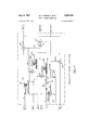
- FIG. 2 is a diagrammatic view of a basic rate computing loop embodying the present invention
- FIG. 3 is a curve showing the relationship of the time constant Tc to the computed rate in the basic rate computing loop of FIG. 2;
- FIG. 4 is a diagrammatic view of an electrical circuit which is the equivalent of the basic rate computing loop of FIG. 2;
- FIG. 5 is a curve illustrating the frequency response of the electrical circuit of FIG. 4;
- FIG. 6 is a curve illustrating the weighting function of the basic rate computing loop of FIG. '2;
- FIG. 7 is a curve illustrating the weighting function of the basic rate computing loop of FIG. 2 in combination with an acceleration smoothing network illustrated in FIG. 15;
- FIG. 8 is a block diagram of a linear rates network forming part of the prediction system of the present invention.
- FIG. 9 is a block diagram of a Q computer constituting part of the linear rates network shown in FIG 8;
- FIG. 10 is a block diagram of a deflection rate computer constituting part of the linear rates network shown in FIG. 8;
- FIG. 11 is a diagram of the deflection rate computer of FIG. 10, but showing the components in greater detail;
- FIG. 12 is a diagram illustrating the effect of changes in B, the true target bearing, upon Xt, the lateral component of target velocity, measured perpendicular to the line of sight and upon Yt, the horinzontal line of sight component of target velocity;
- FIG. 13 is a diagram illustrating the effect of changes in B upon dH, the rate of climb or vertical component of target velocity
- FIG. 14 is a block diagram of a height and horizontal range rate computer constituting part of the linear rates network shown in FIG. 8;
- FIG. is a block diagram of an acceleration smoothing network forming part of the prediction system of the present invention.
- FIG. 16 is a block diagram of a prediction unit forming part of the prediction system of the present invention.
- FIG. 17 is a diagram illustrating geometric errors encountered with linear prediction involving a constant time constant Tc
- FIG. 18 is a diagram illustrating geometric errors encountered with linear prediction involving a constant a
- FIG. 19 is a diagram illustrating geometric errors encountered with curvilinear predition involving a constant time constant To and constant acceleration constant K;
- FIG. 20 is a diagram illustrating geometric errors encountered with curvilinear prediction involving a constant time constant To and an acceleration constant equal to l 22;
- FIG. 21 is a diagram illustrating geometric errors encountered with curvilinear prediction involving constant 25 and acceleration constant equal to l 22.
- A--Target angle Angle between vertical plane through the relative target speed vector, and the vertical plane through the line of sight, measured in the horizontal plane clockwise from the target speed vector.
- B-True target bearing Angle between the north-south vertical plane through the line of sight, measured in the horizontal plane. Positive angles measured clockwise from north.
- BrDirector train Angle between the vertical plane through own ship centerline, and the vertical plane through the line of sight, measured in the deck plane. Positive angles measured clockwise from own ship centerline.
- BrRelative target bearing Angle between the vertical plane through own ship centerline, and the vertical plane through the line of sight, measured in the horizontal plane. Positive angles measured clockwise from own ship centerline.
- C0Own ship course Angle between the north-south vertical plane, and the vertical plane through own ship speed vector (referred to the plane used by the fire control system), measured in the horizontal plane. Positive angles measured clockwise from north.
- Ct-Target course Angle between the northsouth vertical plane, and the vertical plane through the target speed vector (referred to the frame used by the fire control system), measured in the horizontal plane. Positive angle measured clockwise from north.
- Dh-Horizontal deflection prediction Angle between the vertical plane through the line of sight and the vertical plane through the line of fire, measured in the horizontal plane from the vertical plane through the line of sight.
- Dt-Sight deflection The part of sight deflection accounting for relative motion between own ship and target. (The lateral component or the component at right angles to line of sight of target movement during the time of flight.)
- DtoDeflection preditions The horizontal deflection (linear) due to relative motion of ship and target during time of flight.
- d-When added before a quantity indicates the diflerential operator A-When added before a quantity, indicates a small change or increment of that quantity.
- E-Target elevation or position angle Angle between the horizontal plane and the line of sight, measured in the vertical plane through the line of sight. Positive angles measured upward from the horizontal plane.
- Eli-Director elevation Angle between the deck plane and the line of sight, measured in the vertical plane through the line of sight. Positive angles measured upward from the deck plane.
- EgVertical gun elevation Angle between the horizontal plane and the line of fire, measured in the vertical plane through the line of fire. Positive angles measured upward from the horizontal plane.
- EZ-Future target elevation or ballistic position angle Angle between the horizontal plane and the line to the future target position, measured in the vertical plane through the line to the future target position. Positive angles measured upward from the horizontal plane.
- dH-Vertical linear movement or rate of climb Vertical linear displacement during the time of flight in the vertical plane through the line of sight, due to relative motion between own ship and target in the frame used by the fire control system (vertical component of target velocity).
- Ht The vertical component of target movement during the time of flight.
- R-Present range The distance from own ship (gun director) to target measured along the line of sight.
- RlzHorizonta1 range Projection of present range in the horizontal plane by a vertical plane through the line of sight Rh: R cos E.
- RtRange spot The difference between present range and future range (the horizontal line of sight component of target movement during the time of flight).
- RtoRange prediction The horizontal range component of the relative motion of ship and target during time of flight.
- R2-Advance or ballistic range The distance from own ship to the advance position measured along the line to the advance position.
- ShHcrizontal angular movement or target speed Angle between the vertical plane through the line of sight, and the vertical plane through the line to the future target position, measured in the horizontal plane from the vertical plane through the line of sight.
- S0Linear movement in horizontal or ship speed The linear displacement during the time of flight in the horizontal plane and in the vertical plane through the relative target speed vector in the frame used by the fire control system (due to own ship motion).
- Sw-Horizontal true wind speed The rate of the true wind in the horizontal plane and in the vertical plane through the total true wind speed vector, measured with respect to the earth.
- T-Time Clock time.
- TcComputer time constant The time in seconds for an error in the computation of a rate to decay to l/e of its original value, where e is the base of natural logarithms.
- TdDelay time The time in seconds between present computed data and the past input data that corresponds with the present computed data.
- Time of flight The time of flight of the projectile to the future target position.
- X0Linear movement in bearing The linear displacement during the time of flight in the horizontal plane perpendicular to the vertical plane through the line of sight, resulting from relative motion between own ship and target in the frame used by the fire control system (the lateral component of ship motion or relative wind, measured perpendicular to the line of sight),
- Y0Linear movement in bearing The linear displacement during the time of flight in the horizontal plane and in the vertical plane through the line of sight, due to relative motion, between own ship and target in the frame used by the fire control system (the horizontal line of sight component of ship motion or relative wind),
- the target is predicted to travel either along a straight line, along a parabola line or along any one of a family of courses between said lines, depending upon the K setting (acceleration constant) of the system. Prediction is based upon the linear velocity and acceleration of the target, as determined from the components of acceleration measured along and perpendicular to the present line of sight. It is assumed that the target will retain its present acceleration for seconds, and that target velocity will vary from the present value according to the assumed constant acceleration. After 10 seconds, the target velocity is assumed to be constant.
- Perturbations are generally present in the target data supplied by the director, due to tracking irregularities. With no smoothing, the target velocity and acceleration computed from these data would contain greatly amplified perturbations creating so-called noise errors. If these noise were ignored, the resulting dispersion would place the target at widely scattered points. Consequently, smoothing is introduced into the system.
- the smoothing as will be more fully described, will be of the exponential second derivative type.
- a prediction network including the prediction unit of FIG. 16 predicts what the target path will be depending upon the value of K introduced in the acceleration smoothing network (FIG. 15) and predicts where the target will be Tf seconds in the future, Tf being the time required for a projectile, fired at the present moment, to reach this future target position. After this point is located, the prediction network transforms this information into useable dimensions.
- K introduces compensation for the inherent delay time of the linear rates network. This delay in a rate solution results whenever the target changes course or speed and corresponds to a time in the past when the true rates had the same values as the present computed rates, assuming constant acceleration.
- the instantaneous future horizontal range rate of target movement will therefore be the algebraic sum of its present range rate (yt) and of its present range acceleration dyt multiplied by T7, or Yt+ (dyt)Tf.
- the average rate will be Yt+ /2 (dyt) T
- the horizontal range distance (Rt) traveled by the target during T is the product of its average range rate and T1 or In like manner, expressions may be derived for the defiection Dt and height Ht components of target move ment.
- Equations 7 and 14 If Equations 7 and 14 are combined, a single equation for the target motion range prediction Rt and the range effect of gun motion R0 can be obtained as follows:
- the outputs of the prediction unit FIG. 16 are combined with other quantities to form the required ballistic range R2, ballistic position angle E2, vertical gun elevation Eg, and horizontal deflection Dlz.
- Position angle E i.e. the angle between the line of sight and the horizontal plane, measured in a vertical plane
- R the angle between the line of sight and the horizontal plane, measured in a vertical plane
- dRItYO YZ (12)
- R/zdB is the linear deflection rate
- X0 is the lateral component of ship motion or relative wind, measured perpendicular to the line of sight
- Y0 is the horizontal line of sight component of ship motion or relative wind.
- the present position network is not shown but this network converts the polar coordinates Er, Eli and R obtained from the gun director into a stable system of polar coordinates B, E and Rh whose values do not change with the rolling, pitching and changes in course of own ship and supplies these converted quantities as inputs into linear rates network shown in FIG. 8.
- Br is the director train, or the angle between the vertical plane through the ships centerline and the vertical plane through the line of sight, measured in the deck plane clockwise from the bow
- Eb is the director elevation or the angle between the line of sight and the deck plane, measured in the vertical plane through the line of sight
- R is the present target range or the distance from the gun director to the target.
- the apparent wind network which is also not shown, supplies to the linear rates network, the components of own ship velocity, X0 and Y0.
- One of the networks employed in the target predicting system of the present invention is the linear rates notwork (FIG. 8) which computes the values of some of the quantities in Equations 1, '2. and 3 and makes them available to the acceleration smoothing network (FIG. 15) and t0 the prediction unit (FIG. 16).
- This linear rates network takes input B, E. R, R]: from the present position network (not shown), X0 and Y0 from the apparent wind network (not shown) and Tf from the ballistic network (not shown), and from these inputs computes for the acceleration smoothing network (FIG. 15) and prediction unit (FIG. 16), the quantities d8, time rate change of the true bearing of the target; RhdB,
- the acceleration smoothing network (FIG. 15) to solve Equations 1, 2 and 3.
- This latter network computes from these quantities, smoothed acceleration components of target motion relative to the line of sight.
- the specific quantities computed by the acceleration smoothing network are Kdxt, the product of the acceleration constant K and the smoothed lateral acceleration of target relative to the line of sight; Ka'(dh), the product of the acceleration constant K and the smoothed vertical acceleration of the target; and Kd(yt), the product of the acceleration constant K and the smoothed horizontal acceleration of target in the plane of sight.
- the K constant in the above quantities has the effect of compensating for the time delay Ta of the linear rates network.
- This time delay Td is the time in seconds between the present computed data and the past input data that corresponds with the present computed data assuming constant acceleration for the future prediction period. This delay in a rate solution results whenever the target changes course or speed.
- the linear rates network smooths invariant rates, that is, rates which do not vary with time providing the target moves at a constant speed along a straight path. This type of smoothing has the advantage of minimizing the rate errors. Since invariant rates change slowly or not at all, the time delay inherent in smoothing has small eifect on the accuracy of rate computations.
- RATE COMPUTING LOOP One of the rate computing loops employed in the linear rates network is illustrated in basic form in FIG. 2 for the computation, for example, of angular bearing rate dBc.
- This loop utilizes a mechanical integrator of the well-known type arranged in a loop circuit, so that it operates as a diflerentiator.
- This mechanical intcgrator is shown of the well-known mechanical disc type. in this description, the letter 0 will be used to distinguish computed quantities from inputs.
- a time motor (not shown) drives the integrator disc 10 at a constant speed, so that the revolutions of the disc represent time (T).
- a differential 11 compares the output hell of the integrator roller 12 with the target bearing B whose rate is to be computed.
- the difference jB between B and A03 turns a gearing 13 of ratio Q.
- the output of this gearing 13 connects with the integrator carriage 14. and moves the carriage so as to reduce the difference. It will be shown that the position dBc of the carriage 14 closely represents the rate of change of B.
- Equation 13 Differentiating Equation 13 with respect to time, to express it in more convenient form,
- Equation 14 shows that if Q is very large, dBc very nearly equals dB. Q is commonly called the sensitivity since it is a measure of the sensitiveness of dBc to changes in dB.
- Equation 14 The error in dBc, the computed bearing rate, is shown by Equation 14 to be:
- Time cnstant The reciprocal of Q is the time constant Tc, which is the time required for the rate error to decrease to 37% of its initial value under the following condition: At an initial time when dBc is correct, dB changes instantaneously from one value to another, and remains at the second value thereafter.
- Equation 14 may be demonstrated as follows: Assume the conditions shown in FIG. 3. The true rate shown by the heavy lines varies as a step function of time. At T equal to zero, dB changes instantaneously from zero to a constant value, C. Also at T equal to zero, dBc is zero, which means that the integrator carriage 14 (FIG. 2) is at the center of the disc 10. Then, for all values of T greater than zero, Equation 14 can be rewritten:
- Ta is a measure of the time required to obtain a rate solution. It also is a measure of the amount of smoothing introduced in the rate networks.
- the integrator loops that compute bearing, elevation, and range rates are designed for data smoothing as well as rate computing. This feature is necessary to obtain smooth gun orders.
- Target position data may contain minor perturbations due to imperfect tracking as already described. These in turn may be so magnified in the prediction computations that they cause undue roughness in gun orders. For example, assume an input:
- CT true target bearing as a function of time
- a sin wT represents a perturbation of amplitude A and angular frequency w.
- D in B is simply dB(Tf).
- D CTf+(wA cos wT)Tf (15) Note that the resulting perturbation in D is Tf(w) times as large as A sin wT. For this reason, it is necessary to smooth either the present position data or the computed rates and accelerations, or both.
- the computer smooths the computed rates, and accelerations. Since smoothing usually introduces a time delay, smoothing is used only where essential; that is, where perturbations of input data are most likely to cause perturbations of the computed outputs.
- the basic loop (FIG. 2) is analagous to the electrical network shown in FIG. 4, which consists of a perfect rate computer followed by an RC filter,
- Equation 15 Since the amplitude of perturbations in prediction (Equation 15) is proportional to T the necessary amount of smoothing is also proportional to Tf. Accordingly, To is made proportional to T7 for constant sigma 22 operation, where sigma 2 is defined as Tc /Tf.
- Weighting function The filtering or smoothing action of the rate computing loop can be expressed in terms of its transient response (FIG. 3), its frequency response (FIG. 5), or its weighting function (FIG. 6), all of which are interdependent.
- the weighting function expresses the memory of the loop. It indicates the extent by which past input data afiect present computations.
- the weighting function (FIG. 6) has the form of a single exponential curve. A change in input at any past time has an efiect, or weight, on the present computed rate that is expressed by the ordinate of the curve for that past time. The curve shows that recent data are Weighed most heavily.
- the acceleration smoothing network (FIG. 15) of itself produces the same smooth ng action as the rate computing loop of FIG. 2.
- two smoothing actions are involved in the computation of accelerations.
- the first smoothing action takes place in the rate computing loop and the second smoothing action takes place in the acceleration smoothing network.
- the weighting function that characterizes the overall acceleration smoothing is therefore represented by a double exponential curve (FIG. 7).
- jXr is the correction due to changes in target speed or course in AXt, the generated lateral component of target bearing; jYt is the correction due to changes in target speed or course in AYt, the generated line of sight component of target velocity due to changes in target bearing and jdH is the correction due to changes in targe speed or course in AdH, the generated vertical component of target velocity due to changes in target hearing.
- Td is the abscissa of the centroid of the area under the weighting function curve (FIG. 6).
- Ta is defined as the time delay in the computation of accelerations [d(xt, d(yt), and d(dh)] if the target has a constant rate of change of acceleration.
- the value of Td for the acceleration smoothing network has the following relation to the value of Tc for the rate computing loops, as shown in FIG. 7
- FIG. 8 shows the linear rates network in block diagrammatic form.
- the major units of this linear rates network are the Q computer (FIG. 9), the deflection rate computer (FIGS. 10 and 11) and the height and horizontal range computer (FIG. 14).
- the Q" computer is one of the major units of the linear rates network.
- This Q computer shown in FIG. 9 receives an input of time of flight Ti and from this furnishes an output Q.
- the computer sensitivity Q is the reciprocal of the time constant Tc (smoothing delay time) of the linear rate network, where Tc is the time required for the error to decrease to 37% of its in; al value.
- Tc smoothing delay time
- the time constant Tc may be determined either manually or automatically. When Tc is adjusted manually, it may be limited, for example, to values between 1 second and 29 seconds for anti-aircraft control and between 5 seconds and 100 seconds for surface control.
- the time constant of the network is controlled automatically. It can be varied in proportion to time of flight T (constant 2 operation where Tc 2 Tf or it can be set at a fixed optimum value (constant Q operation). During the first few seconds of tracking, the time constant is automatically reduced to obtain a quick solution.
- the value of Ti obtained from the ballistic network (not shown) is converted into its reciprocal l/Tj by a non-linear potentiometer 19.
- Q is computed to maintain a constant sigma by two potentiometers 20 and 21 and to obtain a low-valued initial sigma and a high-valued steady state sigma under constant sigma conditions.
- the potentiometer 20 used during the initial tracking period is adjustable, for example, to a lower limit of 0.1 sigma.
- the other potentiometer 21, used thereafter, can be separately adjusted, for example, to a lower limit of 0.1 sigma, although it is intended that the steady state sigma shall be four times the initial sigma.
- a potentiometer 23 is provided to maintain a constant Tc, the value of which is determined by adjustment.
- Q is computed by a potentiometer 24 to maintain a constant sigma, adjustable, for example, to a lower limit of 0.2.
- a hand selector switch 255 permits selection between a Q with constant sigma and a Q with constant Tc and a control switch 26 permits selective setting for an antiaircraft Q or for a surface Q.
- DEFLECTION RATE COMPUTER The deflection rate computer of FIGS. 10 and 11, constituting part of the linear rates network of FIG. 8 cmbodies the principles of the basic rate computing loop shown in FIG. 2 and already described.
- this computer the true target bearing B obtained from the present position network (not shown) and the time T obtained from a time motor, are combined in a differential 30 and an integrator 31 to obtain jB, the change in bearing angle (i.e. angular correction).
- jB drives the disc of an integrator 32, while Q from the Q computer of FIG. 9 is made to change the gear ratio to the carriage of said integrator.
- This arrangement permits the introduction of various sensitivity constants Q to satisfy different smoothing and sensitivity constants.
- the roller output of the integrator 32 namely jBc, the change in computed bearing rate (rate correction) is impressed upon the disc of an inte rator 33, while Rh is impressed upon the carriage of said integrator 33 to obtain the quantity jXt, which is the target deflection rate due to a change in target motion.
- An integrator 34 serves to generate AXt, the change in Xt due to changes in target bearing, Xt being the defiection component of target motion.
- B is fed into the disc of the integrator 34, while Yl, the horizontal line of sight component of target velocity is fed into the carriage of this integrator.
- the theory of operr" n of this integrator 34 is as follows: Since the horizontal components (FIG. 12) of target velocity are measured relative to the line of sight, trey must vary with changes in B. That is not true of the vertical component did, as shown by FIG. 13. Assuming that the target moves in a straight line at a constant speed, S11 and Cl remain constant.
- AXt represents the change in X1 due to changes in target bearing
- any other changes in (RhdB-Xo) obtained from a differential 35 must be due to a change in target motion from its assumed constant speed and linear course.
- the target deflection rate due to this change in target motion, and called jXt generated by the integrator 33 is combined with AXt in a differential 36 to form X1 and also turns the rotor of a generator 37, whose voltage output represents QdjXt, the deflection component of target acceleration.
- This generator 37 is so designed, that its voltage output is proportional to the product of its field voltage Q, and the rate of change, d(Xt), or its mechanical input jXt.
- This accelerat on component Qdt(jXz) is supplied to the acceleration smoothing network (FIG. 15).
- This quantity RhdB as well as Rh obtained from the present position network (not shown) are introduced into a divider 38 to obtain dB which serves to move the carriage of the integrator 31 and thereby to correct the position of said carriage, until it represents a smoothed value of dB.
- the quantity RhdB from the differential 35 and the quantity Xt from the differential 36 are not only fed back into the system, as described, but are delivered in conjunction with the quantity Qd(jXt) to the acceleration smoothing network (FIG. 15).
- the quantity Q is applied to the quantity jXt which is the rate correction to AXz for changes in target speed or course, so that smoothing acts upon this correction.
- This quantity jXt is a rate which does not change with time, if target speed and course remain constant and therefore is an invariant rate.
- the quantity AXt is the generated lateral component of target velocity due to changes in target bearing and since the target bearing is continuously changing, even though the course of the target and its speed is constant, this quantity is a variant rate. Since the variant portion AXt of Xt is supplied by the integrator 34, the remainder of the loop is concerned only with the computation of jXt. Smoothing introduced by the rate computing loop, therefore, acts solely upon the invariant rate jXt and the rate error caused by smoothing is consequently reduced.
- HEIGHT AND HORIZONTAL RANGE RATE COMPUTER In general, the function of the height and horizontal range rate computer shown in FIG. 14 is the same as that already described for the deflection rate computer of FIGS. 10 and 11. The main differences are in the number of units which must be inserted in the response line from the comparison differential to the integrator carriage to obtain the desired quantities. Since this height and horizontal range rate computer is similar to the 14 deflection rate network of FIGS. 10 and 11, it will be only briefly described herein and only in connection with a block diagram.
- the present target range R obtained from the :gun director and the time T obtained from a time motor are combined in a differential 40 and an integrator 41 to obtain jdR.
- the quantity jdR modified in an integrator by gear ratio correction Q from the Q computer of FIG. 9, is delivered to a component integrator 43 in conjunction with the position angle E derived from the present position network (not shown), to obtain the functions jdR cos E and MR sin E.
- the position angle E and the time T are combined in a differential 44 and an integrator 45 to obtain 'E which is modified by the present target range R in an integrator 46 to produce the quantity 'RdE.
- This latter quantity after modification by the gear ratio Q in an integrator 47 is delivered to a component integrator 48 to obtain the functions jRdE cos E and jRdE sin E.
- This output dH is multiplied by the sensitivity coeflicient Q in a generator 50 to obtain the quantity Qd(dI-I) for delivery to the acceleration smoothing network (FIG. 15) and is also made available to the prediction unit (FIG. 16).
- the quantity jRa'E sin E from the component integrator 48 and the quantity jdR cos E from the component integrator 43 are fed into a differential 51 to obtain the quantity 'Y t.
- This quantity jYt and the quantity Q delivered to a generator 52 generates the quantity Qd( 'Yt) which is one of the quantities desired for delivery to the accelerating smoothing network (FIG. 15).
- This quantity AYt compared with the quantity jYt from the differential 51 produces in a differential 54 the quantity Yt which is returned to the integrator 34 of the deflection rate computer of FIGS. '10 and 11 for the purpose already described.
- This quantity Yt is also delivered to a differential 55 in conjunction with the quantity Yo derived from the apparent wind network (not shown) to obtain the quantity dRh which goes into a resolver 57 in conjunction with the position angle E, to obtain the functions dRh sin E and (IR cos E.
- a resolver 58 With inputs E and dH, generates functions dH cos E and dH sin E. One of these quantities dH sin E and the quantity dRh cos E from the resolver 57 are compared in a differential 60 to produce dR which is fed back into the integrator 41. The other quantity dH cos E from the resolver 58 is compared in a differential 61 with the quantity dRh sin E from the resolver 57 to generate the quantity RdE. This quantity RdE delivered to a divider 62 in conjunction with the present target range R produces the quantity dE which is fed back into the integrator 45.
- This quantity iYt is a rate which does not change with time, if target speed and course remain constant and therefore is an invariant rate.
- the quantity AYt is a generated line of sight component of target velocity due to changes in target bearing, and since the target bearing is continuously changing even though the course of the target and its speed is constant, this quantity is a variant rate. Since the variant rate portion AYz' of Yt is supplied by the integrator 53, the
Landscapes
- Engineering & Computer Science (AREA)
- General Engineering & Computer Science (AREA)
- Feedback Control In General (AREA)
Description
Aug. 8, 1961 w. H. NEWELL ET AL TARGET COURSE PREDICTOR Filed April 22, 1954 k4 l/EET/CAL PAR/IA 4 AX 401v Maw/v7;
BASE
D/FFfEE/VT/AL l|| llllllllllllllllllllll'llllll 13 Sheets-Sheet l M/TfGEATO/Q 5145/6 R14 75 COMPUT/NG LOOP INVENTORS Wag.
Aug. 8, 1961 w. H. NEWELL ETAL 2,995,296
TARGET COURSE PREDICTOR l3 Sheets-Sheet 4 Filed April 22, 1954 QwwEEQQ mg 3% Q? ND xQmQ 2st um FGQ Re E \ER um TMQ ATTORNEY w. H. NEWELL ETAL 2,995,296
TARGET COURSE PREDICTOR 13 Sheets-Sheet 5 Aug. 8, 1961 Filed April 22, 1954 I INVENTORS W/LL/AMH MEWELL J GEORGE A. (Eda/THEE By W (1 w A TTOR NE 1' 8, 1961 w. H. NEWELL ET AL 2,995,296
TARGET COURSE PREDICTOR l3 Sheets-Sheet 6 Filed April 22. 1954 INVENTORS j QQQSS M/IL LIAN/K IVE WELL G-fOEGE Aug. 8, 1961 w. H. NEWELL ET AL 2,995,296
TARGET COURSE PREDICTOR Filed April 22, 1954 13 Sheets-Sheet 7 m mm mm. \N.
m A r\ km NXN Q U W NX X n Av mum Aug. 8, 1961 w. H. NEWELL ET AL 2,995,296
TARGET COURSE PREDICTOR Filed April 22, 1954 13 Sheets-Sheet 9 1961 w. H. NEWELL ETAL 2,995,296
TARGET COURSE PREDICTOR INV'ENT-ORS 13 Sheets-Sheet l1 W. H. NEWELL ET AL TARGET COURSE PREDICTOR w QhEQm Aug. 8, 1961 Filed April 22, 1954 /1 TTORNE Y United States Patent 2,995,296 TARGET COURSE PREDICTOR William H. Newell, Mount Vernon, and George A. 'Crowther, Manhasset, N.Y., assignors to Sperry Rand Corporation, a corporation of Delaware Filed Apr. 22, 1954, Ser. No. 424,814
18 Claims. (Cl. 235-615) The present invention relates to a target course predictor for a gun fire control system and to certain component parts, per se, of said predictor.
A linear predictor in the absence of tracking errors will predict correctly the motion of a target moving with constant linear velocity and a curvilinear predictor in the absence of tracking errors will predict correctly the motion of a target, even when accelerating, as long as the target acceleration along any fixed cartesian coordinate axis is constant. If the target has a changing acceleration, due, for example, to the maneuvering of the target, then it is impossible to foretell exactly what the target will do at some future time. Some intelligent assump tions, therefore, must be made concerning the targets future path, to attain a high incidence of predicting accuracy.
The present data obtained from the director of the gun fire control system for course prediction computations contain a certain amount of noise due to tracking irregularities. If this noise were ignored, the resulting dispersion would place the projectiles at widely scattered points. For this reason, smoothing must be introduced into the system. If smoothing were applied directly to the present position data, which is usually changing rather fast, the resulting quantities would lag the correct data a considerable amount. For this reason, smoothing is applied in accordance with the present invention, to quantities which do not change very often, namely, to the quantities which change only when the target changes its course or speed.
As the amount of smoothing is increased, the dispersion due to noise decreases. However, the geometrical errors (i.e., errors due to target manuvering) introduced by using smoothed rates, increase. In accordance with the present invention, the targets acceleration is assumed to remain constant during the time of flight.
.This means that if the target has a constant velocity or a constant acceleration, the predictor will predict its future position with practically no error. If, however, the target has a changing acceleration, the predictions are based on a velocity and an acceleration that existed some time in the past depending on the amount of smoothing which is applied to the target rates.
For a given set of conditions (radar, director, computer, target maneuverability, time of flight, etc.) there is some optimum amount of smoothing which will result in the greatest chance of hitting the target.
One object of the present invention is to provide a new and improved target course predictor, which will aiford the optimum amount of smoothing under the conditions present, and which will thereby predict automatically the course of a target moving with constant linear velocity, constant acceleration or varying acceleration, with sutiicient accuracy to provide a comparatively high probability of hitting the target.
Another object of the present invention is to provide a new and improved target course predictor, sufiiciently flexible to solve with a high degree of accuracy the problems presented by various targets and tactical situations.
A further object of the present invention is to provide a new and improved target course predictor operable to permit its use effectively and selectively in connection with a surface target or with an airborne target travelling at high speed and allowing therefore little time for engagement.
Another object of the present invention is to provide a new and improved target course predictor, which can be set up for special operation during the acquisition or initial phase of each engagement, when quick solutions are required, and which is automatically switched-over after a predetermined initial period for steady operations.
A further object of the present invention is to provide new and improved component networks for the curved course predictor of the present invention described.
Another object of the present invention is to provide a new and improve rate control loop, which through the expediency of basically an integrator, a differential and a device for introducing a sensitivity coefficient, determines continuously and accurately smoothed rate values.
In solving the prediction problems of the present invention, various relationships may be obtained between noise errors and geometrical errors by varying a computer time constant Tc applied to the target rates for smoothing. This time constant Tc may be constant or may be controlled to afford a constant sigma equal to T c/ T f, where T is the time of flight of the target. To eliminate the lag in the smoothed velocity, an acceleration constant K is employed varying between 0 and 1.4. This K under certain optimum conditions is set to equal 1-1-22.
Various other objects of the invention are apparent from the following particular description and from inspection of the accompanying drawings, in which:
FIG. 1 is a diagram illustrating the prediction problem involved in the present invention;
FIG. 2 is a diagrammatic view of a basic rate computing loop embodying the present invention;
FIG. 3 is a curve showing the relationship of the time constant Tc to the computed rate in the basic rate computing loop of FIG. 2;
FIG. 4 is a diagrammatic view of an electrical circuit which is the equivalent of the basic rate computing loop of FIG. 2;
FIG. 5 is a curve illustrating the frequency response of the electrical circuit of FIG. 4;
FIG. 6 is a curve illustrating the weighting function of the basic rate computing loop of FIG. '2;
FIG. 7 is a curve illustrating the weighting function of the basic rate computing loop of FIG. 2 in combination with an acceleration smoothing network illustrated in FIG. 15;
FIG. 8 is a block diagram of a linear rates network forming part of the prediction system of the present invention;
FIG. 9 is a block diagram of a Q computer constituting part of the linear rates network shown in FIG 8;
FIG. 10 is a block diagram of a deflection rate computer constituting part of the linear rates network shown in FIG. 8;
FIG. 11 is a diagram of the deflection rate computer of FIG. 10, but showing the components in greater detail;
FIG. 12 is a diagram illustrating the effect of changes in B, the true target bearing, upon Xt, the lateral component of target velocity, measured perpendicular to the line of sight and upon Yt, the horinzontal line of sight component of target velocity;
FIG. 13 is a diagram illustrating the effect of changes in B upon dH, the rate of climb or vertical component of target velocity;
FIG. 14 is a block diagram of a height and horizontal range rate computer constituting part of the linear rates network shown in FIG. 8;
FIG. is a block diagram of an acceleration smoothing network forming part of the prediction system of the present invention;
FIG. 16 is a block diagram of a prediction unit forming part of the prediction system of the present invention;
FIG. 17 is a diagram illustrating geometric errors encountered with linear prediction involving a constant time constant Tc;
FIG. 18 is a diagram illustrating geometric errors encountered with linear prediction involving a constant a FIG. 19 is a diagram illustrating geometric errors encountered with curvilinear predition involving a constant time constant To and constant acceleration constant K;
FIG. 20 is a diagram illustrating geometric errors encountered with curvilinear prediction involving a constant time constant To and an acceleration constant equal to l 22;
FIG. 21 is a diagram illustrating geometric errors encountered with curvilinear prediction involving constant 25 and acceleration constant equal to l 22.
GLOSSARY OF TERMS Herein is the glossary of terms herein employed, unless otherwise indicated. The glossary is indicated herein in connection with a gun fire control system on a ship but it must be understood that the invention is not limited in certain of its aspects to a system so located.
A--Target angle: Angle between vertical plane through the relative target speed vector, and the vertical plane through the line of sight, measured in the horizontal plane clockwise from the target speed vector.
B-True target bearing: Angle between the north-south vertical plane through the line of sight, measured in the horizontal plane. Positive angles measured clockwise from north.
BrDirector train (stabilized sight): Angle between the vertical plane through own ship centerline, and the vertical plane through the line of sight, measured in the deck plane. Positive angles measured clockwise from own ship centerline.
BrRelative target bearing: Angle between the vertical plane through own ship centerline, and the vertical plane through the line of sight, measured in the horizontal plane. Positive angles measured clockwise from own ship centerline.
C0Own ship course: Angle between the north-south vertical plane, and the vertical plane through own ship speed vector (referred to the plane used by the fire control system), measured in the horizontal plane. Positive angles measured clockwise from north.
Ct-Target course: Angle between the northsouth vertical plane, and the vertical plane through the target speed vector (referred to the frame used by the fire control system), measured in the horizontal plane. Positive angle measured clockwise from north.
Dh-Horizontal deflection prediction: Angle between the vertical plane through the line of sight and the vertical plane through the line of fire, measured in the horizontal plane from the vertical plane through the line of sight.
Dt-Sight deflection: The part of sight deflection accounting for relative motion between own ship and target. (The lateral component or the component at right angles to line of sight of target movement during the time of flight.)
DtoDeflection preditions: The horizontal deflection (linear) due to relative motion of ship and target during time of flight.
d-When added before a quantity, indicates the diflerential operator A-When added before a quantity, indicates a small change or increment of that quantity.
E-Target elevation or position angle: Angle between the horizontal plane and the line of sight, measured in the vertical plane through the line of sight. Positive angles measured upward from the horizontal plane.
Eli-Director elevation: Angle between the deck plane and the line of sight, measured in the vertical plane through the line of sight. Positive angles measured upward from the deck plane.
EgVertical gun elevation: Angle between the horizontal plane and the line of fire, measured in the vertical plane through the line of fire. Positive angles measured upward from the horizontal plane.
EZ-Future target elevation or ballistic position angle: Angle between the horizontal plane and the line to the future target position, measured in the vertical plane through the line to the future target position. Positive angles measured upward from the horizontal plane.
HTarget height: The height of the target above the horizontal plane measured in the vertical plane through the line of sight H=R sin E.
dH-Vertical linear movement or rate of climb: Vertical linear displacement during the time of flight in the vertical plane through the line of sight, due to relative motion between own ship and target in the frame used by the fire control system (vertical component of target velocity).
d(dh)Smoothed vertical acceleration of target.
HtThe vertical component of target movement during the time of flight.
HZ-Predicted target height.
KAcceleration constant.
QSensitivity coefficient: The reciprocal of the rate time constant Q=1/ T c.
R-Present range: The distance from own ship (gun director) to target measured along the line of sight.
RlzHorizonta1 range: Projection of present range in the horizontal plane by a vertical plane through the line of sight Rh: R cos E.
RtRange spot: The difference between present range and future range (the horizontal line of sight component of target movement during the time of flight).
RtoRange prediction: The horizontal range component of the relative motion of ship and target during time of flight.
R2-Advance or ballistic range: The distance from own ship to the advance position measured along the line to the advance position.
ShHcrizontal angular movement or target speed: Angle between the vertical plane through the line of sight, and the vertical plane through the line to the future target position, measured in the horizontal plane from the vertical plane through the line of sight.
S0Linear movement in horizontal or ship speed: The linear displacement during the time of flight in the horizontal plane and in the vertical plane through the relative target speed vector in the frame used by the fire control system (due to own ship motion).
Sw-Horizontal true wind speed: The rate of the true wind in the horizontal plane and in the vertical plane through the total true wind speed vector, measured with respect to the earth.
T-Time: Clock time.
TcComputer time constant: The time in seconds for an error in the computation of a rate to decay to l/e of its original value, where e is the base of natural logarithms.
TdDelay time: The time in seconds between present computed data and the past input data that corresponds with the present computed data.
T Time of flight: The time of flight of the projectile to the future target position.
X0Linear movement in bearing: The linear displacement during the time of flight in the horizontal plane perpendicular to the vertical plane through the line of sight, resulting from relative motion between own ship and target in the frame used by the fire control system (the lateral component of ship motion or relative wind, measured perpendicular to the line of sight),
XtI.inear movement in hearing: The linear displacement during the time of flight in the horizontal plane perpendicular to the vertical plane through the line of sight, resulting from relative motion between own ship and target in the frame used by the fire control system (the lateral component of target velocity, measured perpendicw lar to the line of sight) Xt=AXt+jXt.
AXt-The operated lateral component of target velocity due to changes in target bearing.
jXt-Correctin to AXt for changes in target speed or course.
d(xt)-Smoothed lateral acceleration of target relative to the line of sight.
Y0Linear movement in bearing: The linear displacement during the time of flight in the horizontal plane and in the vertical plane through the line of sight, due to relative motion, between own ship and target in the frame used by the fire control system (the horizontal line of sight component of ship motion or relative wind),
YtLinear movement in horizontal range: The linear movement during the time of flight in the horizontal plane and in the vertical plane through the line of sight, due to relative motion, between own ship and target in the frame used by the fire control system (the horizontal line of sight component of target velocity), Yt=AYt+jYL AYtThe generated line of sight component of target velocity due to changes in target bearing.
{Yr-Correction to AYt for changes in target course or speed.
d(yt)-Smo0thed horizontal acceleration of target in plane of sight.
In the system of the present invention, the target is predicted to travel either along a straight line, along a parabola line or along any one of a family of courses between said lines, depending upon the K setting (acceleration constant) of the system. Prediction is based upon the linear velocity and acceleration of the target, as determined from the components of acceleration measured along and perpendicular to the present line of sight. It is assumed that the target will retain its present acceleration for seconds, and that target velocity will vary from the present value according to the assumed constant acceleration. After 10 seconds, the target velocity is assumed to be constant.
Perturbations are generally present in the target data supplied by the director, due to tracking irregularities. With no smoothing, the target velocity and acceleration computed from these data would contain greatly amplified perturbations creating so-called noise errors. If these noise were ignored, the resulting dispersion would place the target at widely scattered points. Consequently, smoothing is introduced into the system. The smoothing, as will be more fully described, will be of the exponential second derivative type.
EQUATIONS INVOLVED IN THE PREDICTION PROBLEM It can be shown that in order to obtain double exponential smoothing of second derivative values, the smoothed accelerations must satisfy the differential equations These equations are solved for the smoothed lateral acceleration (dxt), the smoothed horizontal acceleration (dyt) and the smoothed vertical acceleration d(dh) in an acceleration smoothing network shown in FIG. 15. In these formulas, the rate of change of the acceleration terms d(dxt), d(dyt) and d (dh) contribute the smoothing. The terms dB(dyt) and dB(dxt) compensate for changes in the acceleration components (dxt) and (dyt) respectively, due to the changing position of the line of sight.
Dividers in the acceleration smoothing network remove the sensitivity coefiicient Q appearing before each acceleration quantity in the above equations. Subsequently, the smoothed accelerations are multiplied by K, to obtain outputs to a prediction unit (FIG. 16).
A prediction network including the prediction unit of FIG. 16 predicts what the target path will be depending upon the value of K introduced in the acceleration smoothing network (FIG. 15) and predicts where the target will be Tf seconds in the future, Tf being the time required for a projectile, fired at the present moment, to reach this future target position. After this point is located, the prediction network transforms this information into useable dimensions.
As will be more fully described, the value of K introduces compensation for the inherent delay time of the linear rates network. This delay in a rate solution results whenever the target changes course or speed and corresponds to a time in the past when the true rates had the same values as the present computed rates, assuming constant acceleration.
As already described, predictions are based on the assumption that the target will retain its present acceleration for ten seconds and that during this time its instantaneous velocity will vary from its present velocity according to this assumed constant acceleration. For any value of Ti less than ten seconds, the instantaneous future horizontal range rate of target movement will therefore be the algebraic sum of its present range rate (yt) and of its present range acceleration dyt multiplied by T7, or Yt+ (dyt)Tf. During this time, the average rate will be Yt+ /2 (dyt) T The horizontal range distance (Rt) traveled by the target during T is the product of its average range rate and T1 or In like manner, expressions may be derived for the defiection Dt and height Ht components of target move ment.
The range (Rt), deflection (Dr) and height (Ht) predictions to compensate for target movement during the time of flight are shown in FIG. 1. When T is less than ten seconds, the target motion predictions are based on the following equations, which are equation of parabolas:
The expressions for the range R0 and deflection Do corrections to compensate for gun motion (exclusive of relative wind) are as follows:
D0: (X0) (Tf) If Equations 7 and 14 are combined, a single equation for the target motion range prediction Rt and the range effect of gun motion R0 can be obtained as follows:
f)+ (y J) If Rto is substituted for (RH-Ro and dRh for (Yo+ Y1), the following expression for Rto may be obtained:
f)+ (y f) Similarly, the deflection correction for gun motion (Do) (Equation 8) and the deflection prediction for tar- 7 get motion (Dt) (Equation may be combined to give the following expression for (Dto) The prediction unit (FIG. 16) computes R10, Dto, and Ht according to Equations 9, and 6 respectively.
The outputs of the prediction unit FIG. 16 are combined with other quantities to form the required ballistic range R2, ballistic position angle E2, vertical gun elevation Eg, and horizontal deflection Dlz.
QUANTITIES REQUlRED FOR SOLUTION PREDICTION PROBLEM From Equations 1, 2, 3, 6, 9 and 10, it is apparent that to solve the prediction problem, it is necessary to compute the following quantities: dB, RirdB, Rh, XI, Qzi(jXt), dH, Qd(dH), Yr, QdjYt, (ZR/z and Q.
Position angle E, i.e. the angle between the line of sight and the horizontal plane, measured in a vertical plane, is combined in a resolver with the present range R from the gun director to form the horizontal range R11 and height H according to the following equations RI1:R cos E H =R sin E The quantity R is therefore required and the quantity E needs to be computed to solve the prediction problem. Further equations to be mechanized for solution of the prediction problem are as follows:
dRItYO=YZ (12) where R/zdB is the linear deflection rate, X0 is the lateral component of ship motion or relative wind, measured perpendicular to the line of sight and Y0 is the horizontal line of sight component of ship motion or relative wind. The quantities X0 and Y0, therefore, must be rendered continuously available for solution of the preiction problem.
The present position network is not shown but this network converts the polar coordinates Er, Eli and R obtained from the gun director into a stable system of polar coordinates B, E and Rh whose values do not change with the rolling, pitching and changes in course of own ship and supplies these converted quantities as inputs into linear rates network shown in FIG. 8. Br is the director train, or the angle between the vertical plane through the ships centerline and the vertical plane through the line of sight, measured in the deck plane clockwise from the bow; Eb is the director elevation or the angle between the line of sight and the deck plane, measured in the vertical plane through the line of sight; R is the present target range or the distance from the gun director to the target. 13 is the true target hearing or the angle between true north and the vertical plane through the line of sight, measured in the horizontal plane clockwise from true north; E is the position angle or the angle between the line of sight and the horizontal plane, measured in a vertical plane; and R]! is the horizontal range equal to R cos E.
The apparent wind network which is also not shown, supplies to the linear rates network, the components of own ship velocity, X0 and Y0.
One of the networks employed in the target predicting system of the present invention is the linear rates notwork (FIG. 8) which computes the values of some of the quantities in Equations 1, '2. and 3 and makes them available to the acceleration smoothing network (FIG. 15) and t0 the prediction unit (FIG. 16). This linear rates network takes input B, E. R, R]: from the present position network (not shown), X0 and Y0 from the apparent wind network (not shown) and Tf from the ballistic network (not shown), and from these inputs computes for the acceleration smoothing network (FIG. 15) and prediction unit (FIG. 16), the quantities d8, time rate change of the true bearing of the target; RhdB,
the linear deflection rate of the target which is the prodnot of the present horizontal target range Rlz and the time rate of change of the present true bearing dB; Xt, the lateral component of the present target velocity measured perpendicular to the line of sight; Qzl(jXl), the deflection component of target acceleration, the quantity Q being the sensitivity constant and the reciprocal of the rate time constant Tc, to be more fully described; ([H, the rate of climb or vertical component of target velocity; Qd(dH), the component of vertical acceleration of the target; Y1, the horizontal line of sight component of target velocity; Qd(jYt), the horizontal target range acceleration; dR/z, the rate of change of horizontal target range; Q, the sensitivity constant; and
the reciprocal of the time of flight which is the time required for a projectile fired at the persent time to reach the future target position.
The output quantities Qd(jXt), Qd(jYt), Qd(dll), Q,
and dB from the linear rates network (FIG. 8) are received in the acceleration smoothing network (FIG. 15) to solve Equations 1, 2 and 3. This latter network computes from these quantities, smoothed acceleration components of target motion relative to the line of sight. As already pointed out, the specific quantities computed by the acceleration smoothing network are Kdxt, the product of the acceleration constant K and the smoothed lateral acceleration of target relative to the line of sight; Ka'(dh), the product of the acceleration constant K and the smoothed vertical acceleration of the target; and Kd(yt), the product of the acceleration constant K and the smoothed horizontal acceleration of target in the plane of sight. The K constant in the above quantities has the effect of compensating for the time delay Ta of the linear rates network. This time delay Td is the time in seconds between the present computed data and the past input data that corresponds with the present computed data assuming constant acceleration for the future prediction period. This delay in a rate solution results whenever the target changes course or speed.
The linear rates network smooths invariant rates, that is, rates which do not vary with time providing the target moves at a constant speed along a straight path. This type of smoothing has the advantage of minimizing the rate errors. Since invariant rates change slowly or not at all, the time delay inherent in smoothing has small eifect on the accuracy of rate computations.
RATE COMPUTING LOOP One of the rate computing loops employed in the linear rates network is illustrated in basic form in FIG. 2 for the computation, for example, of angular bearing rate dBc. This loop utilizes a mechanical integrator of the well-known type arranged in a loop circuit, so that it operates as a diflerentiator. This mechanical intcgrator is shown of the well-known mechanical disc type. in this description, the letter 0 will be used to distinguish computed quantities from inputs. A time motor (not shown) drives the integrator disc 10 at a constant speed, so that the revolutions of the disc represent time (T). A differential 11 compares the output hell of the integrator roller 12 with the target bearing B whose rate is to be computed. The difference jB between B and A03 turns a gearing 13 of ratio Q. The output of this gearing 13 connects with the integrator carriage 14. and moves the carriage so as to reduce the difference. It will be shown that the position dBc of the carriage 14 closely represents the rate of change of B.
Since the disc 10 of the integrator is driven at constant speed, the speed of its roller 12 is proportional to the displacement of its carriage 14 from the center of the disc. Expressed mathematically,
d (AcB =dBc where AcB is the roller output and d is the differential operator d/dT. The constant proportionality has been omitted for simplicity. Integrating this equation,
ACB C This is the mathematical expression for the roller output. Difiference jB, computed at the differential output, is defined by the relation:
'B :B AcB fdBc Gear ratio Q establishes the relation:
dBc=QjB=QB-QfdBc (13) Differentiating Equation 13 with respect to time, to express it in more convenient form,
d Bc=QdBQdBc Solving for dBc,
dBc=dBZ (d Bc) 14 Equation 14 shows that if Q is very large, dBc very nearly equals dB. Q is commonly called the sensitivity since it is a measure of the sensitiveness of dBc to changes in dB.
The error in dBc, the computed bearing rate, is shown by Equation 14 to be:
Error in dBc= d Bc The error is proportional to the rate of change of dBc, that is, the rate of movement of the integrator carriage 14 (FIG. 2). Compensation is made for this error by computing a correction +l/Q(d Bc) in the acceleration smoothing network (FIG. 15) and adding this correction to the acceleration term used in parabolic prediction. Equations 1, 2 and 3 solved in the acceleration smoothing network (FIG. 15) involve this compensation.
Time cnstant.The reciprocal of Q is the time constant Tc, which is the time required for the rate error to decrease to 37% of its initial value under the following condition: At an initial time when dBc is correct, dB changes instantaneously from one value to another, and remains at the second value thereafter.
The relation:
may be demonstrated as follows: Assume the conditions shown in FIG. 3. The true rate shown by the heavy lines varies as a step function of time. At T equal to zero, dB changes instantaneously from zero to a constant value, C. Also at T equal to zero, dBc is zero, which means that the integrator carriage 14 (FIG. 2) is at the center of the disc 10. Then, for all values of T greater than zero, Equation 14 can be rewritten:
dBc: C'%(d Bc) This linear diiierential equation has for its solution under the assumed initial conditions.
dBc=C(le- Where e is 2.7183 the base of natural logarithms. When T equals l/Q,
dBc=C(1---eor, since e equals 2.7183,
dBc=63% of C and Error in dBc=37% of C Hence, by definition, Tc equals 1/ Q.
Since the computer has provision for setting and indicating Tc rather than Q, Tc will be used in the remaining description in place of 1/ Q. From the foregoing it may be evident that Ta is a measure of the time required to obtain a rate solution. It also isa measure of the amount of smoothing introduced in the rate networks.
The integrator loops that compute bearing, elevation, and range rates are designed for data smoothing as well as rate computing. This feature is necessary to obtain smooth gun orders.
Target position data may contain minor perturbations due to imperfect tracking as already described. These in turn may be so magnified in the prediction computations that they cause undue roughness in gun orders. For example, assume an input:
where CT represents true target bearing as a function of time, and A sin wT represents a perturbation of amplitude A and angular frequency w. Also, assume that the predicted change D in B is simply dB(Tf).
Then,
D=CTf+(wA cos wT)Tf (15) Note that the resulting perturbation in D is Tf(w) times as large as A sin wT. For this reason, it is necessary to smooth either the present position data or the computed rates and accelerations, or both.
The computer smooths the computed rates, and accelerations. Since smoothing usually introduces a time delay, smoothing is used only where essential; that is, where perturbations of input data are most likely to cause perturbations of the computed outputs.
Smoothing action of basic rate computing l00p.The basic loop (FIG. 2) is analagous to the electrical network shown in FIG. 4, which consists of a perfect rate computer followed by an RC filter,
where Ei corresponds to B E corresponds to dB E0 corresponds to dBc RC corresponds to Tc Smoothing takes place in the RC filter which has the frequency characteristic shown in the curve of FIG. 5, the abscissa of which is on a logaritlnnetic scale. High frequency variations of B, which may be perturbations, are attenuated while low frequency variations of B due to normal changes in target data, are passed with little attenuation. Increasing Tc causes increased attenuation, predominately at the higher frequencies. Therefore, the amount of smoothing is proportional to Tc.
Since the amplitude of perturbations in prediction (Equation 15) is proportional to T the necessary amount of smoothing is also proportional to Tf. Accordingly, To is made proportional to T7 for constant sigma 22 operation, where sigma 2 is defined as Tc /Tf.
Weighting function.-The filtering or smoothing action of the rate computing loop can be expressed in terms of its transient response (FIG. 3), its frequency response (FIG. 5), or its weighting function (FIG. 6), all of which are interdependent. The weighting function expresses the memory of the loop. It indicates the extent by which past input data afiect present computations. For the rate computing loop, the weighting function (FIG. 6) has the form of a single exponential curve. A change in input at any past time has an efiect, or weight, on the present computed rate that is expressed by the ordinate of the curve for that past time. The curve shows that recent data are Weighed most heavily.
The acceleration smoothing network (FIG. 15) of itself produces the same smooth ng action as the rate computing loop of FIG. 2. However, with respect to the input data B, true target bearing, E, the position angle, and R, the range, two smoothing actions are involved in the computation of accelerations. The first smoothing action takes place in the rate computing loop and the second smoothing action takes place in the acceleration smoothing network. The weighting function that characterizes the overall acceleration smoothing is therefore represented by a double exponential curve (FIG. 7).
Delay zime.Because present computed rates are affected by past data, the present computed rates do not correspond with the present input data but may equal instead the true rate values that existed some time in the past. changing, there is a time lag in the computation of these rates. jXr is the correction due to changes in target speed or course in AXt, the generated lateral component of target bearing; jYt is the correction due to changes in target speed or course in AYt, the generated line of sight component of target velocity due to changes in target bearing and jdH is the correction due to changes in targe speed or course in AdH, the generated vertical component of target velocity due to changes in target hearing. if
these rates jXt, jYt and jdlt are changing uniformly (i.e.
the target has constant acceleration), the time between the present moment and that instant in the past when the true rates were equal to the present computed rates, is known as the delay time Td. Mathematically, Td is the abscissa of the centroid of the area under the weighting function curve (FIG. 6). For the rate computing loop therefore,
T d=Tc However, the computed rates are brought up to date by the addition of rate corrections in the acceleration smoothing network.
For the acceleration smoothing network (FIG. 15), Ta is defined as the time delay in the computation of accelerations [d(xt, d(yt), and d(dh)] if the target has a constant rate of change of acceleration. The value of Td for the acceleration smoothing network has the following relation to the value of Tc for the rate computing loops, as shown in FIG. 7
Unlike rates, no corrections are made to bring the computed accelerations up to date. The computed accelerations, therefore, approximate the true values that existed 2T0 seconds in the past.
FIG. 8 shows the linear rates network in block diagrammatic form. The major units of this linear rates network are the Q computer (FIG. 9), the deflection rate computer (FIGS. 10 and 11) and the height and horizontal range computer (FIG. 14).
Q COMPUTER As was previously pointed out, the Q" computer is one of the major units of the linear rates network. This Q computer shown in FIG. 9 receives an input of time of flight Ti and from this furnishes an output Q. As already indicated, the computer sensitivity Q is the reciprocal of the time constant Tc (smoothing delay time) of the linear rate network, where Tc is the time required for the error to decrease to 37% of its in; al value. The time constant Tc may be determined either manually or automatically. When Tc is adjusted manually, it may be limited, for example, to values between 1 second and 29 seconds for anti-aircraft control and between 5 seconds and 100 seconds for surface control.
To provide adequate smoothing with the least time delay, the time constant of the network is controlled automatically. it can be varied in proportion to time of flight T (constant 2 operation where Tc 2 Tf or it can be set at a fixed optimum value (constant Q operation). During the first few seconds of tracking, the time constant is automatically reduced to obtain a quick solution.
Whenever the target rate jXt, jYr and jdI-l are In the Q computer (FIG. 9), the value of Ti obtained from the ballistic network (not shown) is converted into its reciprocal l/Tj by a non-linear potentiometer 19. For anti-aircraft control, Q is computed to maintain a constant sigma by two potentiometers 20 and 21 and to obtain a low-valued initial sigma and a high-valued steady state sigma under constant sigma conditions. The potentiometer 20 used during the initial tracking period, is adjustable, for example, to a lower limit of 0.1 sigma. The other potentiometer 21, used thereafter, can be separately adjusted, for example, to a lower limit of 0.1 sigma, although it is intended that the steady state sigma shall be four times the initial sigma. An adjustable time delay relay 22, controlled by the director switch (not shown) which controls the computer time motors, determines the time of transfer from initial to steady state sigma. If this time switch is open, the relay 22 connects the Q line to obtain a low-valued sigma. Closing the switch changes the connection, after a few seconds delay, to obtain a high valued sigma to control the linear rates network.
Also, for anti-aircraft control, a potentiometer 23 is provided to maintain a constant Tc, the value of which is determined by adjustment.
For surface control, Q is computed by a potentiometer 24 to maintain a constant sigma, adjustable, for example, to a lower limit of 0.2.
A hand selector switch 255 permits selection between a Q with constant sigma and a Q with constant Tc and a control switch 26 permits selective setting for an antiaircraft Q or for a surface Q.
DEFLECTION RATE COMPUTER The deflection rate computer of FIGS. 10 and 11, constituting part of the linear rates network of FIG. 8 cmbodies the principles of the basic rate computing loop shown in FIG. 2 and already described. In this computer, the true target bearing B obtained from the present position network (not shown) and the time T obtained from a time motor, are combined in a differential 30 and an integrator 31 to obtain jB, the change in bearing angle (i.e. angular correction). jB drives the disc of an integrator 32, while Q from the Q computer of FIG. 9 is made to change the gear ratio to the carriage of said integrator. This arrangement permits the introduction of various sensitivity constants Q to satisfy different smoothing and sensitivity constants. The roller output of the integrator 32, namely jBc, the change in computed bearing rate (rate correction) is impressed upon the disc of an inte rator 33, while Rh is impressed upon the carriage of said integrator 33 to obtain the quantity jXt, which is the target deflection rate due to a change in target motion.
An integrator 34 serves to generate AXt, the change in Xt due to changes in target bearing, Xt being the defiection component of target motion. For that purpose, B is fed into the disc of the integrator 34, while Yl, the horizontal line of sight component of target velocity is fed into the carriage of this integrator. The theory of operr" n of this integrator 34 is as follows: Since the horizontal components (FIG. 12) of target velocity are measured relative to the line of sight, trey must vary with changes in B. That is not true of the vertical component did, as shown by FIG. 13. Assuming that the target moves in a straight line at a constant speed, S11 and Cl remain constant.
Since Then dA=dB From the right triangle in FIG. 11
Xt=Sh sin A (15) and Yt=Sh cos A (17) 13 Differentiating Equations 16 and 17 d(Xt) =Sh COS AdA d(Yt) =Sh sin AdA Substituting -Yt for Sh cos A, Xt for Sh sin A and dB for dA, we obtain The integrator 34 computes AXt in accordance with Equation 20.
Since AXt represents the change in X1 due to changes in target bearing, any other changes in (RhdB-Xo) obtained from a differential 35 must be due to a change in target motion from its assumed constant speed and linear course. The target deflection rate due to this change in target motion, and called jXt generated by the integrator 33 is combined with AXt in a differential 36 to form X1 and also turns the rotor of a generator 37, whose voltage output represents QdjXt, the deflection component of target acceleration. This generator 37 is so designed, that its voltage output is proportional to the product of its field voltage Q, and the rate of change, d(Xt), or its mechanical input jXt. This accelerat on component Qdt(jXz) is supplied to the acceleration smoothing network (FIG. 15).
The deflection component of target motion Xt from the output of the differential 36 and the lateral component of ship motion X obtained from the apparent wind network (not shown) are compared in the differential 35 to obtain the linear deflection rate RhdB in accordance with the relation RhdB=Xo+Xt (Equation 11), and to isolate Xt. This quantity RhdB as well as Rh obtained from the present position network (not shown) are introduced into a divider 38 to obtain dB which serves to move the carriage of the integrator 31 and thereby to correct the position of said carriage, until it represents a smoothed value of dB.
The quantity RhdB from the differential 35 and the quantity Xt from the differential 36 are not only fed back into the system, as described, but are delivered in conjunction with the quantity Qd(jXt) to the acceleration smoothing network (FIG. 15).
It should be noted that in the deflection rate computer of FIGS. and 11, the quantity Q is applied to the quantity jXt which is the rate correction to AXz for changes in target speed or course, so that smoothing acts upon this correction. This quantity jXt is a rate which does not change with time, if target speed and course remain constant and therefore is an invariant rate. The quantity AXt is the generated lateral component of target velocity due to changes in target bearing and since the target bearing is continuously changing, even though the course of the target and its speed is constant, this quantity is a variant rate. Since the variant portion AXt of Xt is supplied by the integrator 34, the remainder of the loop is concerned only with the computation of jXt. Smoothing introduced by the rate computing loop, therefore, acts solely upon the invariant rate jXt and the rate error caused by smoothing is consequently reduced.
HEIGHT AND HORIZONTAL RANGE RATE COMPUTER In general, the function of the height and horizontal range rate computer shown in FIG. 14 is the same as that already described for the deflection rate computer of FIGS. 10 and 11. The main differences are in the number of units which must be inserted in the response line from the comparison differential to the integrator carriage to obtain the desired quantities. Since this height and horizontal range rate computer is similar to the 14 deflection rate network of FIGS. 10 and 11, it will be only briefly described herein and only in connection with a block diagram.
In this height and horizontal range computer, the present target range R obtained from the :gun director and the time T obtained from a time motor are combined in a differential 40 and an integrator 41 to obtain jdR. The quantity jdR modified in an integrator by gear ratio correction Q from the Q computer of FIG. 9, is delivered to a component integrator 43 in conjunction with the position angle E derived from the present position network (not shown), to obtain the functions jdR cos E and MR sin E.
At the same time, the position angle E and the time T are combined in a differential 44 and an integrator 45 to obtain 'E which is modified by the present target range R in an integrator 46 to produce the quantity 'RdE. This latter quantity after modification by the gear ratio Q in an integrator 47 is delivered to a component integrator 48 to obtain the functions jRdE cos E and jRdE sin E. The quantity jRdE cos E from the component integrator 48 and the quantity jdR sin E from the component integrator 43 are delivered to a differential 49 to obtain the output dH following the relationship H =R sin E. This output dH is multiplied by the sensitivity coeflicient Q in a generator 50 to obtain the quantity Qd(dI-I) for delivery to the acceleration smoothing network (FIG. 15) and is also made available to the prediction unit (FIG. 16).
The quantity jRa'E sin E from the component integrator 48 and the quantity jdR cos E from the component integrator 43 are fed into a differential 51 to obtain the quantity 'Y t. This quantity jYt and the quantity Q delivered to a generator 52 generates the quantity Qd( 'Yt) which is one of the quantities desired for delivery to the accelerating smoothing network (FIG. 15).
The true target bearing B and the quantity Xt obtained from the deflection rate computer of FIGS. 10 and 11 are delivered to an integrator 53 to obtain AYt following Equation 21, namely AYt=fXtdB. This quantity AYt compared with the quantity jYt from the differential 51 produces in a differential 54 the quantity Yt which is returned to the integrator 34 of the deflection rate computer of FIGS. '10 and 11 for the purpose already described. This quantity Yt is also delivered to a differential 55 in conjunction with the quantity Yo derived from the apparent wind network (not shown) to obtain the quantity dRh which goes into a resolver 57 in conjunction with the position angle E, to obtain the functions dRh sin E and (IR cos E. A resolver 58 With inputs E and dH, generates functions dH cos E and dH sin E. One of these quantities dH sin E and the quantity dRh cos E from the resolver 57 are compared in a differential 60 to produce dR which is fed back into the integrator 41. The other quantity dH cos E from the resolver 58 is compared in a differential 61 with the quantity dRh sin E from the resolver 57 to generate the quantity RdE. This quantity RdE delivered to a divider 62 in conjunction with the present target range R produces the quantity dE which is fed back into the integrator 45.
The height and horizontal range computer of FIG. 14, as in the case of the deflection rate computer of FIGS. 10 and 11, embodies the principles of the basic rate computing looping of FIG. 2 described, and applies the quantity Q to quantity of 'Yt which is the rate correction to AYt for changes in target speed or course, so that smoothing acts upon this correction. This quantity iYt is a rate which does not change with time, if target speed and course remain constant and therefore is an invariant rate. The quantity AYt is a generated line of sight component of target velocity due to changes in target bearing, and since the target bearing is continuously changing even though the course of the target and its speed is constant, this quantity is a variant rate. Since the variant rate portion AYz' of Yt is supplied by the integrator 53, the
Priority Applications (1)
| Application Number | Priority Date | Filing Date | Title |
|---|---|---|---|
| US424814A US2995296A (en) | 1954-04-22 | 1954-04-22 | Target course predictor |
Applications Claiming Priority (1)
| Application Number | Priority Date | Filing Date | Title |
|---|---|---|---|
| US424814A US2995296A (en) | 1954-04-22 | 1954-04-22 | Target course predictor |
Publications (1)
| Publication Number | Publication Date |
|---|---|
| US2995296A true US2995296A (en) | 1961-08-08 |
Family
ID=23683982
Family Applications (1)
| Application Number | Title | Priority Date | Filing Date |
|---|---|---|---|
| US424814A Expired - Lifetime US2995296A (en) | 1954-04-22 | 1954-04-22 | Target course predictor |
Country Status (1)
| Country | Link |
|---|---|
| US (1) | US2995296A (en) |
Cited By (2)
| Publication number | Priority date | Publication date | Assignee | Title |
|---|---|---|---|---|
| US4794235A (en) * | 1986-05-19 | 1988-12-27 | The United States Of America As Represented By The Secretary Of The Army | Non-linear prediction for gun fire control systems |
| US7002510B1 (en) * | 1987-01-28 | 2006-02-21 | Raytheon Company | Method and apparatus for air-to-air aircraft ranging |
Citations (9)
| Publication number | Priority date | Publication date | Assignee | Title |
|---|---|---|---|---|
| US2404011A (en) * | 1943-06-21 | 1946-07-16 | Sperry Gyroscope Co Inc | Prediction apparatus |
| US2408081A (en) * | 1941-05-01 | 1946-09-24 | Bell Telephone Labor Inc | Artillery predictor |
| US2435195A (en) * | 1942-06-20 | 1948-02-03 | Bell Telephone Labor Inc | Data smoothing network |
| US2441175A (en) * | 1943-07-30 | 1948-05-11 | Sperry Corp | System for reproducing angular motion at a distance |
| US2602587A (en) * | 1948-11-26 | 1952-07-08 | Sperry Corp | Component resolver |
| US2660371A (en) * | 1943-08-28 | 1953-11-24 | Sperry Corp | Gun directing system |
| US2699895A (en) * | 1943-02-01 | 1955-01-18 | Sperry Corp | Angular rate measuring system |
| US2713457A (en) * | 1950-06-09 | 1955-07-19 | Phillips Petroleum Co | Computer |
| US2754058A (en) * | 1937-05-26 | 1956-07-10 | Sperry Rand Corp | Mechanism for controlling the aiming of ordnance |
-
1954
- 1954-04-22 US US424814A patent/US2995296A/en not_active Expired - Lifetime
Patent Citations (9)
| Publication number | Priority date | Publication date | Assignee | Title |
|---|---|---|---|---|
| US2754058A (en) * | 1937-05-26 | 1956-07-10 | Sperry Rand Corp | Mechanism for controlling the aiming of ordnance |
| US2408081A (en) * | 1941-05-01 | 1946-09-24 | Bell Telephone Labor Inc | Artillery predictor |
| US2435195A (en) * | 1942-06-20 | 1948-02-03 | Bell Telephone Labor Inc | Data smoothing network |
| US2699895A (en) * | 1943-02-01 | 1955-01-18 | Sperry Corp | Angular rate measuring system |
| US2404011A (en) * | 1943-06-21 | 1946-07-16 | Sperry Gyroscope Co Inc | Prediction apparatus |
| US2441175A (en) * | 1943-07-30 | 1948-05-11 | Sperry Corp | System for reproducing angular motion at a distance |
| US2660371A (en) * | 1943-08-28 | 1953-11-24 | Sperry Corp | Gun directing system |
| US2602587A (en) * | 1948-11-26 | 1952-07-08 | Sperry Corp | Component resolver |
| US2713457A (en) * | 1950-06-09 | 1955-07-19 | Phillips Petroleum Co | Computer |
Cited By (2)
| Publication number | Priority date | Publication date | Assignee | Title |
|---|---|---|---|---|
| US4794235A (en) * | 1986-05-19 | 1988-12-27 | The United States Of America As Represented By The Secretary Of The Army | Non-linear prediction for gun fire control systems |
| US7002510B1 (en) * | 1987-01-28 | 2006-02-21 | Raytheon Company | Method and apparatus for air-to-air aircraft ranging |
Similar Documents
| Publication | Publication Date | Title |
|---|---|---|
| US4172409A (en) | Fire control system for vehicle-mounted weapon | |
| US4959800A (en) | Method and apparatus for determining the position and velocity of a target in inertial space | |
| US3575085A (en) | Advanced fire control system | |
| US4494202A (en) | Fourth order predictive, augmented proportional navigation system terminal guidance design with missile/target decoupling | |
| GB1374101A (en) | Aircraft control systems | |
| US2433843A (en) | Fixed gun interaircraft fire control system | |
| US4456862A (en) | Augmented proportional navigation in second order predictive scheme | |
| US3309963A (en) | Fire control system for an antiaircraft weapon carrier | |
| US4146780A (en) | Antiaircraft weapons system fire control apparatus | |
| US3260478A (en) | Method and means for controlling travel motion of an object in dependence upon the position of another object | |
| US4020407A (en) | Control system for tracking a moving target | |
| US2995296A (en) | Target course predictor | |
| US4492352A (en) | Noise-adaptive, predictive proportional navigation (NAPPN) guidance scheme | |
| GB847232A (en) | Rocket launch control system | |
| GB1314741A (en) | Method of controlling motor-driven devices adapted to be directed onto moving targets and apparatus for applying the method | |
| US3699310A (en) | Angular rate bombing system | |
| US3900175A (en) | Guidance system for an anti-aircraft missile | |
| US3156435A (en) | Command system of missile guidance | |
| US4794235A (en) | Non-linear prediction for gun fire control systems | |
| JPS58501688A (en) | Method and apparatus for guiding an aerodynamic object with a homing device | |
| US3206143A (en) | Controller for guiding a missile carrier on the location curve of ballistic firing positions | |
| US3293643A (en) | Fire control system for use on board a ship | |
| US3995144A (en) | Banked bombing system | |
| US2696947A (en) | Gun directing system | |
| Blakelock | Design and analysis of a digitally controlled integrated flight/firecontrol system |