US10417699B2 - Systems and methods for optimal bidding in a business to business environment - Google Patents
Systems and methods for optimal bidding in a business to business environment Download PDFInfo
- Publication number
- US10417699B2 US10417699B2 US15/255,115 US201615255115A US10417699B2 US 10417699 B2 US10417699 B2 US 10417699B2 US 201615255115 A US201615255115 A US 201615255115A US 10417699 B2 US10417699 B2 US 10417699B2
- Authority
- US
- United States
- Prior art keywords
- deals
- price
- distribution
- equation
- parameters
- Prior art date
- Legal status (The legal status is an assumption and is not a legal conclusion. Google has not performed a legal analysis and makes no representation as to the accuracy of the status listed.)
- Active, expires
Links
Images
Classifications
-
- G—PHYSICS
- G06—COMPUTING OR CALCULATING; COUNTING
- G06Q—INFORMATION AND COMMUNICATION TECHNOLOGY [ICT] SPECIALLY ADAPTED FOR ADMINISTRATIVE, COMMERCIAL, FINANCIAL, MANAGERIAL OR SUPERVISORY PURPOSES; SYSTEMS OR METHODS SPECIALLY ADAPTED FOR ADMINISTRATIVE, COMMERCIAL, FINANCIAL, MANAGERIAL OR SUPERVISORY PURPOSES, NOT OTHERWISE PROVIDED FOR
- G06Q30/00—Commerce
- G06Q30/06—Buying, selling or leasing transactions
- G06Q30/08—Auctions
-
- G—PHYSICS
- G06—COMPUTING OR CALCULATING; COUNTING
- G06Q—INFORMATION AND COMMUNICATION TECHNOLOGY [ICT] SPECIALLY ADAPTED FOR ADMINISTRATIVE, COMMERCIAL, FINANCIAL, MANAGERIAL OR SUPERVISORY PURPOSES; SYSTEMS OR METHODS SPECIALLY ADAPTED FOR ADMINISTRATIVE, COMMERCIAL, FINANCIAL, MANAGERIAL OR SUPERVISORY PURPOSES, NOT OTHERWISE PROVIDED FOR
- G06Q30/00—Commerce
- G06Q30/02—Marketing; Price estimation or determination; Fundraising
- G06Q30/0283—Price estimation or determination
Definitions
- the present invention relates to systems and methods for optimally pricing high-volume commercial transactions between businesses, referred to as business-to-business (B2B) pricing.
- B2B business-to-business
- the data is highly heterogeneous, covering thousands of distinct products and buyers. Different product types have different price sensitivities. Consequently, the data contain a large number of “rows” (observed deals) as well as “columns” (explanatory variables). Predictive models may thus be vulnerable to noise accumulation, spurious correlations, and computational issues.
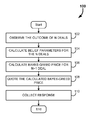
- systems and methods for optimizing bidding in a business-to-business environment are provided. Initially the observed outcomes for n deals are received, and the belief parameters for these n deals are calculated. The Bayes-greedy price is then calculated and presented to a buyer. The buyer's response is collected and an optimal variance parameter based on the buyer's response is generated. The belief parameters for these n+1 deals are also updated. This process may be repeated for additional deals.
- FIG. 1 is a flow diagram of an example process for generating and administering a quote using Bayes-Greedy projections, in accordance with some embodiment.
- FIGS. 2A and 2B are example computer systems capable of implementing the system for improving bidding optimizations, in accordance with some embodiments.
- the presently disclosed systems and methods are directed toward using predictive and prescriptive analytics in B2B pricing.
- Many models in revenue management allow stochastic product demand but in B2B environments case, the seller faces the additional challenge of environmental uncertainty: the seller does not know the exact distribution of the buyer's willingness to pay. Rather, this distribution is estimated from historical data, assuming some statistical model (e.g., logistic regression), and this model is updated over time as new transactions take place. In this way, any given deal provides new information about the demand distribution, aside from its purely economic value in generating revenue. Furthermore, since any given statistical model is likely to be inaccurate, the seller may not wish to implement the price that seems to be optimal under that model.
- the seller may experiment with prices (for instance, charging slightly more or less than the recommended price) in order to obtain new information and potentially discover better pricing strategies. Doing this may result in lost revenue at first, but the new information may help to improve pricing decisions in the (hopefully near) future.
- This problem may be approached from the perspective of optimal learning, which typically uses Bayesian models to measure the uncertainty, or the potential for error, in the predictive model.
- logistic regression with the coefficients modeled as a random vector (because their “true” values are unknown).
- the power of these models comes from the concept of “correlated beliefs”, which measures the similarities and differences between various types of deals, so that a sale involving one product will teach something about other, similar products.
- the Bayesian model can then be integrated with a pricing strategy that accounts for the uncertainty in the model, e.g., by correcting overly aggressive prices when the uncertainty is high, or by experimenting with higher prices when there is a chance that they may be better than we think.
- the outcomes of the decisions feed back into the model and modify beliefs for future decisions.
- This framework can provide meaningful guidance within very short time horizons, even in the presence of very noisy data.
- Optimal learning methods typically use simple Bayesian models that can be updated very quickly.
- linear regression such as least squares
- the standard approach is to assume that the regression coefficients are normally distributed, which enables concise modeling and updating correlated beliefs.
- there is no analogous model for logistic regression making it difficult to represent beliefs about logistic demand curves.
- This problem can be approached using approximate Bayesian inference, and create a new learning mechanism that allows the seller to maintain an update a multivariate normal belief on the regression coefficients using rigorous statistical approximations.
- the seller may then develop a “Bayes-greedy” pricing strategy that optimizes an estimate of expected revenue by averaging over all possible revenue curves.
- the Bayesian framework performs very well in both predictive and prescriptive roles. Surprisingly, despite the approximations used in the Bayesian model, it demonstrates superior predictive power over exact logistic regression. It has been determined that uncertainty is valuable: the benefits of quantifying uncertainty about the predictive model vastly outweigh any reduction in accuracy incurred by using approximations. Not only does the Bayesian model make more accurate predictions of future wins and losses, but the Bayes-greedy policy generates more revenue by integrating the uncertainty directly into the pricing decision.
- this disclosure makes the following contributions: 1) the introduction of a new approximate Bayesian learning model for learning B2B demand curves based on logistic regression.
- the presently disclosed approach optimizes a statistical measure of distance between the multivariate normal approximation and the exact, non-normal posterior distribution. This optimality criterion has great practical significance, as improved performance from the Bayesian model is not seen when it is not used.
- the seller's beliefs can be efficiently updated in this model, using stochastic gradient methods to calculate the optimal statistical approximation. 3)
- the Bayes-greedy pricing policy is presented, and shows how these prices can be efficiently computed.
- x ⁇ R M is a vector that depends on p, as well as on additional characteristics of the product or the buyer, which are known to the seller at the time p is chosen.
- the function ⁇ which is not known exactly to the seller, is also called the demand curve.
- the seller's expected revenue from the deal is given by:
- R ⁇ ( p ; x , ⁇ ) p ⁇ ⁇ ⁇ ( x , ⁇ ) , ⁇ p ⁇ 0 ,
- Equation 1 is an instance of logistic regression, a standard model for forecasting demand or sales.
- x also contains information such as the type and quantity of product stipulated in the deal.
- a large number of dummy variables may be used to describe the product. For example, a large retailer may wish to include features that classify products by department (e.g., electronic, furniture, housewares, etc.), then generally describe the item in question (e.g., TVs, cameras, tablets), and finally give more detailed information such as the brand and model of the item.
- x could describe the buyer with varying degrees of granularity (e.g., whether the buyer is located in Europe or Asia for example, followed by more detailed country information), since B2B pricing is highly individualized. It is also possible to include interaction terms between product and customer features (e.g., if a particular product type sells better in a particular region), as well as interactions between these features and the price (to model the case where different products have different price sensitivities). Since the outcome of B2B negotiations heavily depends on the individual salesperson, x may also include characteristics of the sales force. In a practical application, x may include hundreds or thousands of elements.
- any unknown quantity is modeled as a random variable whose distribution represents our beliefs about likely values for that quantity.
- a multivariate normal prior distribution is used, that is:
- the main benefit of the multivariate normal distribution is that it allows us to compactly represent correlated beliefs using the covariance matrix ⁇ .
- the off-diagonal entries in this matrix can be viewed as representing the degree of similarity or difference between the values of different regression coefficients. Correlations have great practical impact when the design matrix is sparse, that is, many of the components of x are equal to zero for any given observation. This is likely to be the case in our application: the seller may include thousands of distinct products into the model, and only a few observations may be available for a given product even if the overall dataset is large. However, if we believe that two products are similar, correlated beliefs will allow us to learn about one product from a deal that involves the other one. This greatly increases the information value of a single deal, and allows us to learn about a large number of products from a small number of observations. Furthermore, normality assumptions will substantially simplify the computation of optimal prices.
- h ⁇ ( ⁇ , ⁇ , ⁇ ′ ⁇ ⁇ ′ ) 1 2 ⁇ [ tr ⁇ ( ⁇ - 1 ⁇ ⁇ ⁇ ′ ) + ( ⁇ - ⁇ ′ ) T ⁇ ⁇ ⁇ ( ⁇ - ⁇ ′ ) - M - log ⁇ ⁇ ⁇ ′ ⁇ ⁇ ⁇ + C ] . Equation ⁇ ⁇ 6
- C is a constant that does not depend on ⁇ ′, ⁇ ′.
- this model treats ⁇ (Y ⁇ 1 ⁇ 2) as an observation of the log-odds of success for the next deal. Subtracting 1 ⁇ 2 from Y ensures that this observation can be both positive and negative, so that new wins cause us to increase the estimated win probability, while new losses shift the estimate downward. This is in line with the standard interpretation of logistic regression that positive coefficients lead to higher win probabilities.
- the parameter v can be thought of as a user-specified measure of the accuracy of this observation (higher v means lower accuracy).
- v p ⁇ circumflex over ( ) ⁇ (1 ⁇ p ⁇ circumflex over ( ) ⁇ ), where p ⁇ circumflex over ( ) ⁇ is the predicted success probability for the feature vector x using ⁇ as the regression coefficients.
- ⁇ * arg ⁇ ⁇ min , D KL ⁇ ( Q ⁇ P )
- Proposition 2 is provided as:
- the IPA estimator for fixed v can be constructed as follows. Given fixed ⁇ , ⁇ , x, and Y, we calculate ⁇ and ⁇ using equations 10 and 11. Then, we simulate Z ⁇ circumflex over ( ) ⁇ ⁇ N (0, 1) and calculate
- ⁇ ⁇ ⁇ x T ⁇ ⁇ ′ + x T ⁇ ⁇ ′ ⁇ x ⁇ Z ⁇ .
- G ⁇ - ( 2 ⁇ Y - 1 ) ⁇ e - H ⁇ ( ⁇ ⁇ ; Y ) 1 + e - H ⁇ ( ⁇ ⁇ ; Y ) ⁇ [ Y - 1 2 ⁇ x T ⁇ ⁇ ⁇ ⁇ x + x T ⁇ ⁇ ( v + x T ⁇ ⁇ ⁇ ⁇ x ) 2 ⁇ x T ⁇ ⁇ ⁇ x + ( x T ⁇ ⁇ ⁇ ⁇ x ) 2 ( v - x T ⁇ ⁇ ⁇ ⁇ x ) 2 ⁇ Z ⁇ ] .
- equation 6 To obtain the deterministic component, we return to equation 5 and differentiate h.
- the terms in equation 6 can be rewritten as:
- FIG. 1 a flow chart is provided, at 100 , that details the steps taken to optimize the bidding process.
- Y n+1 is the buyer's response.
- the seller's initial beliefs are represented by a multivariate normal distribution with the prior parameters ( ⁇ 0 , ⁇ 0 ), which may be calibrated based on historical data.
- the seller's beliefs are represented (at 104 ) by a multivariate normal distribution with posterior parameters (0 n , ⁇ n ).
- the features x n of the next deal become known to the seller, a price p n is quoted, and the response Y n+1 is observed.
- the parameters of this distribution are obtained from the recursive update equations 10-11, with the variance parameter v computed using the procedure presented previously. We then proceed to the next deal under the assumption that the seller's belief distribution continues to be normal.
- the Bayes-Greed price for the n+1 deal is calculated (at 106 ) as is detailed below in relation to the next two sections.
- the quote is then administered to a buyer (at 108 ) and the buyer's response is collected (at 110 ).
- approximate Bayesian inference is applied sequentially. Every new iteration introduces an additional degree of approximation, but the learning mechanism is computationally efficient, and we maintain the ability to model and update our uncertainty about ⁇ . We now show how price optimization can be integrated into this framework.
- the seller's pricing decisions are adaptive, so that p n may depend on the posterior parameters ( ⁇ n , ⁇ n ), as well as on the other features of x n .
- the seller's decision is to choose a pricing policy, which can be represented as a function ⁇ mapping ( ⁇ n , ⁇ n , x n ) to a price p n ⁇ 0.
- the optimal policy maximizes the objective function:
- equation 15 is intractable even for small N, since our distribution of belief is characterized by M 2 +M continuous parameters, and we have very little information about the process that generates the features x n of each deal. Modeling this process is substantially more difficult than modeling uncertainty about the regression coefficients, and is outside the scope of this paper.
- the regression features are known when we choose the price for the deal, it is possible to design a myopic policy that seeks to maximize the revenue obtained from this deal without looking ahead to future deals.
- Myopic policies have been shown to possess asymptotic optimality properties in some cases. Since we primarily deal with short time horizons in our application, we focus on developing a myopic policy that is computationally tractable and will perform well in practice.
- p * , n arg ⁇ max p ⁇ ⁇ p 1 + ⁇ e ⁇ x n ) T ⁇ ⁇ ,
- ⁇ p n arg ⁇ max p ⁇ ⁇ p 1 + e - ( x n ) T ⁇ ⁇ n , Equation ⁇ ⁇ 16
- ⁇ n is the current vector of regression coefficients. This approach is used in frequentist models, where ⁇ n is computed using maximum likelihood estimation (in other words, frequentist logistic regression). If x n depends linearly on the price, equation 16 has a closed-form expression in terms of the Lambert W function.
- ⁇ p n arg ⁇ max p ⁇ 0 ⁇ E ⁇ n ⁇ ( p 1 + e - ( x n ) T ⁇ ⁇ ) , Equation ⁇ ⁇ 17
- x f is a vector of features whose values are fixed (known to the seller and not dependent on p)
- x p is another fixed vector of features related to the price sensitivity.
- each component of x either depends linearly on p, or does not depend on p at all. In the simplest possible example, may be a dummy variable which equals 1 if the buyer is asking for a certain specific product.
- ⁇ p ⁇ ( x T ⁇ ⁇ + x T ⁇ ⁇ ⁇ ⁇ x ⁇ Z ⁇ ( ⁇ ) ) ( x p ) T ⁇ ⁇ p + ( x p ) T ⁇ ⁇ pf ⁇ x f + p ⁇ ( x p ) T ⁇ ⁇ pp ⁇ x p x T ⁇ ⁇ ⁇ ⁇ x ⁇ Z ⁇ ( ⁇ ) . Equation ⁇ ⁇ 19
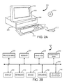
- FIGS. 2A and 2B illustrate a Computer System 200 , which is suitable for implementing embodiments of the present invention.
- FIG. 2A shows one possible physical form of the Computer System 200 .
- the Computer System 200 may have many physical forms ranging from a printed circuit board, an integrated circuit, and a small handheld device up to a huge super computer.
- Computer system 200 may include a Monitor 202 , a Display 204 , a Housing 206 , a Disk Drive 208 , a Keyboard 210 , and a Mouse 212 .
- Disk 214 is a computer-readable medium used to transfer data to and from Computer System 200 .
- FIG. 2B is an example of a block diagram for Computer System 200 . Attached to System Bus 220 are a wide variety of subsystems.
- Processor(s) 222 also referred to as central processing units, or CPUs
- Memory 224 includes random access memory (RAM) and read-only memory (ROM).
- RAM random access memory
- ROM read-only memory
- RAM random access memory
- ROM read-only memory
- Both of these types of memories may include any suitable of the computer-readable media described below.
- a Fixed Disk 226 may also be coupled bi-directionally to the Processor 222 ; it provides additional data storage capacity and may also include any of the computer-readable media described below.
- Fixed Disk 226 may be used to store programs, data, and the like and is typically a secondary storage medium (such as a hard disk) that is slower than primary storage. It will be appreciated that the information retained within Fixed Disk 226 may, in appropriate cases, be incorporated in standard fashion as virtual memory in Memory 224 .
- Removable Disk 214 may take the form of any of the computer-readable media described below.
- Processor 222 is also coupled to a variety of input/output devices, such as Display 204 , Keyboard 210 , Mouse 212 and Speakers 230 .
- an input/output device may be any of: video displays, track balls, mice, keyboards, microphones, touch-sensitive displays, transducer card readers, magnetic or paper tape readers, tablets, styluses, voice or handwriting recognizers, biometrics readers, motion sensors, brain wave readers, or other computers.
- Processor 222 optionally may be coupled to another computer or telecommunications network using Network Interface 240 .
- the Processor 222 might receive information from the network, or might output information to the network in the course of performing the above-described B2B bidding optimization. Furthermore, method embodiments of the present invention may execute solely upon Processor 222 or may execute over a network such as the Internet in conjunction with a remote CPU that shares a portion of the processing.
Landscapes
- Business, Economics & Management (AREA)
- Development Economics (AREA)
- Accounting & Taxation (AREA)
- Finance (AREA)
- Strategic Management (AREA)
- Engineering & Computer Science (AREA)
- Economics (AREA)
- Entrepreneurship & Innovation (AREA)
- Marketing (AREA)
- Physics & Mathematics (AREA)
- General Business, Economics & Management (AREA)
- General Physics & Mathematics (AREA)
- Theoretical Computer Science (AREA)
- Game Theory and Decision Science (AREA)
- Management, Administration, Business Operations System, And Electronic Commerce (AREA)
- Complex Calculations (AREA)
Abstract
Description
and H (β; Y)=(2Y−1)βTx. Then, the posterior density of β can be written as:
x T β˜N(x T θ,x T Σx)
x=[x f ,p·x p]T,
{circumflex over (∇)}p R(p;x,β)
p k+1 =p k+αk{circumflex over (∇)}p
-
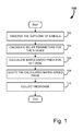
- 1) Apply procedure in equation 20 to find the Bayes-greedy price;
- 2) Implement the price pn that is returned by this procedure (i.e., quote the price to the buyer);
- 3) Observe the
response Y n+1; - 4) Apply procedure of equation 14 to find the optimal variance parameter vn;
- 5) Calculate (θn+1, Σn+1) from equations 10-11.
Claims (7)
Priority Applications (4)
| Application Number | Priority Date | Filing Date | Title |
|---|---|---|---|
| US15/255,115 US10417699B2 (en) | 2015-09-03 | 2016-09-01 | Systems and methods for optimal bidding in a business to business environment |
| PCT/US2016/050299 WO2017041059A2 (en) | 2015-09-03 | 2016-09-03 | Systems and methods for optimal bidding in a business to business environment |
| US16/571,938 US10937087B2 (en) | 2015-09-03 | 2019-09-16 | Systems and methods for optimal bidding in a business to business environment |
| US17/189,735 US20210182953A1 (en) | 2015-09-03 | 2021-03-02 | Systems and methods for optimal bidding in a business to business environment |
Applications Claiming Priority (2)
| Application Number | Priority Date | Filing Date | Title |
|---|---|---|---|
| US201562214193P | 2015-09-03 | 2015-09-03 | |
| US15/255,115 US10417699B2 (en) | 2015-09-03 | 2016-09-01 | Systems and methods for optimal bidding in a business to business environment |
Related Child Applications (1)
| Application Number | Title | Priority Date | Filing Date |
|---|---|---|---|
| US16/571,938 Continuation US10937087B2 (en) | 2015-09-03 | 2019-09-16 | Systems and methods for optimal bidding in a business to business environment |
Publications (2)
| Publication Number | Publication Date |
|---|---|
| US20170091858A1 US20170091858A1 (en) | 2017-03-30 |
| US10417699B2 true US10417699B2 (en) | 2019-09-17 |
Family
ID=58188543
Family Applications (3)
| Application Number | Title | Priority Date | Filing Date |
|---|---|---|---|
| US15/255,115 Active 2037-04-06 US10417699B2 (en) | 2015-09-03 | 2016-09-01 | Systems and methods for optimal bidding in a business to business environment |
| US16/571,938 Expired - Fee Related US10937087B2 (en) | 2015-09-03 | 2019-09-16 | Systems and methods for optimal bidding in a business to business environment |
| US17/189,735 Abandoned US20210182953A1 (en) | 2015-09-03 | 2021-03-02 | Systems and methods for optimal bidding in a business to business environment |
Family Applications After (2)
| Application Number | Title | Priority Date | Filing Date |
|---|---|---|---|
| US16/571,938 Expired - Fee Related US10937087B2 (en) | 2015-09-03 | 2019-09-16 | Systems and methods for optimal bidding in a business to business environment |
| US17/189,735 Abandoned US20210182953A1 (en) | 2015-09-03 | 2021-03-02 | Systems and methods for optimal bidding in a business to business environment |
Country Status (2)
| Country | Link |
|---|---|
| US (3) | US10417699B2 (en) |
| WO (1) | WO2017041059A2 (en) |
Families Citing this family (1)
| Publication number | Priority date | Publication date | Assignee | Title |
|---|---|---|---|---|
| US20220019920A1 (en) * | 2020-07-16 | 2022-01-20 | Raytheon Company | Evidence decay in probabilistic trees via pseudo virtual evidence |
Citations (3)
| Publication number | Priority date | Publication date | Assignee | Title |
|---|---|---|---|---|
| US20040215550A1 (en) * | 2002-12-17 | 2004-10-28 | Hewlett-Packard Development Company, L.P. | Simultaneous purchasing and selling of goods and services in auctions |
| US20090144101A1 (en) * | 2007-11-30 | 2009-06-04 | Sap Ag | System and Method Determining Reference Values of Sensitivities and Client Strategies Based on Price Optimization |
| US8396814B1 (en) * | 2004-08-09 | 2013-03-12 | Vendavo, Inc. | Systems and methods for index-based pricing in a price management system |
-
2016
- 2016-09-01 US US15/255,115 patent/US10417699B2/en active Active
- 2016-09-03 WO PCT/US2016/050299 patent/WO2017041059A2/en not_active Ceased
-
2019
- 2019-09-16 US US16/571,938 patent/US10937087B2/en not_active Expired - Fee Related
-
2021
- 2021-03-02 US US17/189,735 patent/US20210182953A1/en not_active Abandoned
Patent Citations (3)
| Publication number | Priority date | Publication date | Assignee | Title |
|---|---|---|---|---|
| US20040215550A1 (en) * | 2002-12-17 | 2004-10-28 | Hewlett-Packard Development Company, L.P. | Simultaneous purchasing and selling of goods and services in auctions |
| US8396814B1 (en) * | 2004-08-09 | 2013-03-12 | Vendavo, Inc. | Systems and methods for index-based pricing in a price management system |
| US20090144101A1 (en) * | 2007-11-30 | 2009-06-04 | Sap Ag | System and Method Determining Reference Values of Sensitivities and Client Strategies Based on Price Optimization |
Also Published As
| Publication number | Publication date |
|---|---|
| US20210182953A1 (en) | 2021-06-17 |
| US10937087B2 (en) | 2021-03-02 |
| US20200013114A1 (en) | 2020-01-09 |
| US20170091858A1 (en) | 2017-03-30 |
| WO2017041059A2 (en) | 2017-03-09 |
Similar Documents
| Publication | Publication Date | Title |
|---|---|---|
| Chen et al. | Network revenue management with online inverse batch gradient descent method | |
| US20230297847A1 (en) | Machine-learning techniques for factor-level monotonic neural networks | |
| Ursu et al. | The sequential search model: A framework for empirical research: R. Ursu et al. | |
| US9760802B2 (en) | Probabilistic recommendation of an item | |
| US9852193B2 (en) | Probabilistic clustering of an item | |
| CN102402569A (en) | Rating prediction device, rating prediction method, and program | |
| US20240355091A1 (en) | Techniques to perform global attribution mappings to provide insights in neural networks | |
| US20250013939A1 (en) | Method and system for optimizing an objective heaving discrete constraints | |
| US20210272195A1 (en) | Instant Lending Decisions | |
| Peña et al. | Empirical dynamic quantiles for visualization of high-dimensional time series | |
| Hull | Machine learning for economics and finance in TensorFlow 2 | |
| Qu et al. | Learning demand curves in B2B pricing: A new framework and case study | |
| Schürch et al. | Correlated product of experts for sparse Gaussian process regression | |
| Omay et al. | The comparison of power and optimization algorithms on unit root testing with smooth transition | |
| Shi et al. | What, why, and how: An empiricist’s guide to double/debiased machine learning | |
| US10937087B2 (en) | Systems and methods for optimal bidding in a business to business environment | |
| Duan et al. | Sequential Monte Carlo optimization and statistical inference | |
| Ishigaki et al. | Personalized market response analysis for a wide variety of products from sparse transaction data | |
| Chen et al. | Model‐based clustering of regression time series data via APECM—An AECM algorithm sung to an even faster beat | |
| CN116304607A (en) | Automated Feature Engineering for Predictive Modeling Using Deep Reinforcement Learning | |
| Damasceno et al. | Exploiting sparsity and statistical dependence in multivariate data fusion: an application to misinformation detection for high-impact events | |
| CN112381314A (en) | Model training method, model training device, risk prediction method, risk prediction device, electronic equipment and storage medium | |
| CN112529636A (en) | Commodity recommendation method and device, computer equipment and medium | |
| CN114676936A (en) | Method for predicting default time and related device | |
| CN114331500A (en) | Click-through rate prediction method, apparatus, device, storage medium and program product |
Legal Events
| Date | Code | Title | Description |
|---|---|---|---|
| STPP | Information on status: patent application and granting procedure in general |
Free format text: FINAL REJECTION MAILED |
|
| STPP | Information on status: patent application and granting procedure in general |
Free format text: DOCKETED NEW CASE - READY FOR EXAMINATION |
|
| STPP | Information on status: patent application and granting procedure in general |
Free format text: NOTICE OF ALLOWANCE MAILED -- APPLICATION RECEIVED IN OFFICE OF PUBLICATIONS |
|
| AS | Assignment |
Owner name: VENDAVO, INC., CALIFORNIA Free format text: ASSIGNMENT OF ASSIGNORS INTEREST;ASSIGNORS:BERGERSON, ERIC;KURKA, MEGAN;QU, HUASHUAI;AND OTHERS;SIGNING DATES FROM 20120907 TO 20190623;REEL/FRAME:050001/0833 |
|
| STPP | Information on status: patent application and granting procedure in general |
Free format text: PUBLICATIONS -- ISSUE FEE PAYMENT RECEIVED |
|
| STPP | Information on status: patent application and granting procedure in general |
Free format text: PUBLICATIONS -- ISSUE FEE PAYMENT VERIFIED |
|
| STCF | Information on status: patent grant |
Free format text: PATENTED CASE |
|
| AS | Assignment |
Owner name: GOLUB CAPITAL MARKETS LLC, AS COLLATERAL AGENT, ILLINOIS Free format text: PATENT SECURITY AGREEMENT;ASSIGNOR:VENDAVO, INC.;REEL/FRAME:057500/0598 Effective date: 20210910 |
|
| FEPP | Fee payment procedure |
Free format text: MAINTENANCE FEE REMINDER MAILED (ORIGINAL EVENT CODE: REM.); ENTITY STATUS OF PATENT OWNER: LARGE ENTITY |
|
| FEPP | Fee payment procedure |
Free format text: SURCHARGE FOR LATE PAYMENT, LARGE ENTITY (ORIGINAL EVENT CODE: M1554); ENTITY STATUS OF PATENT OWNER: LARGE ENTITY |
|
| MAFP | Maintenance fee payment |
Free format text: PAYMENT OF MAINTENANCE FEE, 4TH YEAR, LARGE ENTITY (ORIGINAL EVENT CODE: M1551); ENTITY STATUS OF PATENT OWNER: LARGE ENTITY Year of fee payment: 4 |