EP4583025A1 - Computation program, computation method, and information processing device - Google Patents
Computation program, computation method, and information processing device Download PDFInfo
- Publication number
- EP4583025A1 EP4583025A1 EP22957288.8A EP22957288A EP4583025A1 EP 4583025 A1 EP4583025 A1 EP 4583025A1 EP 22957288 A EP22957288 A EP 22957288A EP 4583025 A1 EP4583025 A1 EP 4583025A1
- Authority
- EP
- European Patent Office
- Prior art keywords
- objective
- optimal solutions
- optimization
- solutions
- intersects
- Prior art date
- Legal status (The legal status is an assumption and is not a legal conclusion. Google has not performed a legal analysis and makes no representation as to the accuracy of the status listed.)
- Pending
Links
Images





Classifications
-
- G—PHYSICS
- G06—COMPUTING OR CALCULATING; COUNTING
- G06F—ELECTRIC DIGITAL DATA PROCESSING
- G06F17/00—Digital computing or data processing equipment or methods, specially adapted for specific functions
- G06F17/10—Complex mathematical operations
- G06F17/11—Complex mathematical operations for solving equations, e.g. nonlinear equations, general mathematical optimization problems
-
- G—PHYSICS
- G06—COMPUTING OR CALCULATING; COUNTING
- G06F—ELECTRIC DIGITAL DATA PROCESSING
- G06F30/00—Computer-aided design [CAD]
- G06F30/20—Design optimisation, verification or simulation
-
- G—PHYSICS
- G06—COMPUTING OR CALCULATING; COUNTING
- G06Q—INFORMATION AND COMMUNICATION TECHNOLOGY [ICT] SPECIALLY ADAPTED FOR ADMINISTRATIVE, COMMERCIAL, FINANCIAL, MANAGERIAL OR SUPERVISORY PURPOSES; SYSTEMS OR METHODS SPECIALLY ADAPTED FOR ADMINISTRATIVE, COMMERCIAL, FINANCIAL, MANAGERIAL OR SUPERVISORY PURPOSES, NOT OTHERWISE PROVIDED FOR
- G06Q10/00—Administration; Management
- G06Q10/04—Forecasting or optimisation specially adapted for administrative or management purposes, e.g. linear programming or "cutting stock problem"
-
- G—PHYSICS
- G06—COMPUTING OR CALCULATING; COUNTING
- G06Q—INFORMATION AND COMMUNICATION TECHNOLOGY [ICT] SPECIALLY ADAPTED FOR ADMINISTRATIVE, COMMERCIAL, FINANCIAL, MANAGERIAL OR SUPERVISORY PURPOSES; SYSTEMS OR METHODS SPECIALLY ADAPTED FOR ADMINISTRATIVE, COMMERCIAL, FINANCIAL, MANAGERIAL OR SUPERVISORY PURPOSES, NOT OTHERWISE PROVIDED FOR
- G06Q10/00—Administration; Management
- G06Q10/06—Resources, workflows, human or project management; Enterprise or organisation planning; Enterprise or organisation modelling
- G06Q10/063—Operations research, analysis or management
- G06Q10/0639—Performance analysis of employees; Performance analysis of enterprise or organisation operations
-
- G—PHYSICS
- G16—INFORMATION AND COMMUNICATION TECHNOLOGY [ICT] SPECIALLY ADAPTED FOR SPECIFIC APPLICATION FIELDS
- G16Z—INFORMATION AND COMMUNICATION TECHNOLOGY [ICT] SPECIALLY ADAPTED FOR SPECIFIC APPLICATION FIELDS, NOT OTHERWISE PROVIDED FOR
- G16Z99/00—Subject matter not provided for in other main groups of this subclass
Definitions
- optimization problems in fields of various industries including a manufacturing industry and a distribution industry.
- a relationship between a manufacturing time needed for a certain production plan and a cost generated in proportion to an operation time of a device becomes a trade-off.
- a trade-off that, when the manufacturing time is shortened, an operation time of a legacy device having a high operating cost is increased and a cost is increased, and the like.
- a multi-objective optimization problem for simultaneously optimizing a plurality of objective functions having a trade-off relationship is generally a problem of obtaining a Pareto solution.
- each of the manufacturing time needed for the certain production plan and the cost generated in proportion to the operation time of the device is the objective function.
- An explanatory variable is the production plan, and is, for example, an input order in which each product is input to a production process, or the like.
- the Pareto solution is a solution in which at least one of the plurality of objective functions is superior to those of other optional solutions.
- FIG. 2 is a diagram exemplifying a case where a genetic algorithm is used as an example for the multi-objective optimization engine.
- the genetic algorithm is a method of obtaining a solution such that each objective function is minimized from an initial solution group by incorporating genetic elements.
- directions such as moving from initial solutions to a left side and a lower side correspond to search directions. In such a method, it is often not possible to calculate an exact solution in a real time in a real problem having a large problem scale, and thus, it is needed to calculate a more optimal solution in a finite calculation time.
- each optimal solution of the single-objective optimization as a starting point
- each objective function f n and the linear weighted sum obtained by weighting each objective function in the direction perpendicular to a Pareto front are set as the evaluation functions, and the multi-objective optimization calculation is executed to solve the Pareto solutions.
- the search direction of the optimal solutions is set with the linear weighted sum while minimizing each objective function to solve the true Pareto front.
- the genetic algorithm is used as an optimization algorithm, but the present invention is not limited to this.
- Other optimization algorithms such as evolutionary algorithms may be used.
- the optimization execution unit 20 is an example of an execution unit that calculates single-objective optimal solutions that have better values than initial solutions by executing single-objective optimization by using each of a plurality of objective functions as a first evaluation function for the initial solutions, and executes, by using the single-objective optimal solutions as starting points, multiobjective optimization for a second evaluation function by using, as the second evaluation function, a linear weighted sum obtained by performing weighting for each of the plurality of objective functions according to the single-objective optimal solutions.
Landscapes
- Engineering & Computer Science (AREA)
- Physics & Mathematics (AREA)
- General Physics & Mathematics (AREA)
- Theoretical Computer Science (AREA)
- Business, Economics & Management (AREA)
- Mathematical Physics (AREA)
- Human Resources & Organizations (AREA)
- Computational Mathematics (AREA)
- Data Mining & Analysis (AREA)
- Pure & Applied Mathematics (AREA)
- Mathematical Optimization (AREA)
- Mathematical Analysis (AREA)
- Operations Research (AREA)
- Strategic Management (AREA)
- Economics (AREA)
- General Engineering & Computer Science (AREA)
- Entrepreneurship & Innovation (AREA)
- Development Economics (AREA)
- Software Systems (AREA)
- Databases & Information Systems (AREA)
- Algebra (AREA)
- Tourism & Hospitality (AREA)
- Game Theory and Decision Science (AREA)
- Educational Administration (AREA)
- General Business, Economics & Management (AREA)
- Quality & Reliability (AREA)
- Marketing (AREA)
- Geometry (AREA)
- Computer Hardware Design (AREA)
- Evolutionary Computation (AREA)
- Management, Administration, Business Operations System, And Electronic Commerce (AREA)
Abstract
Description
- The present case relates to an arithmetic program, an arithmetic method, and an information processing device.
- A technique is disclosed for optimizing a plurality of objective functions such as a production cost or a production completion time when an input order of products to a production line is optimized (for example, refer to
Patent Documents 1 to 4). -
- Patent Document 1:
Japanese Laid-open Patent Publication No. 2022-83200 - Patent Document 2:
Japanese Laid-open Patent Publication No. 2002-366587 - Patent Document 3:
US Patent Publication No. 2015/0019173 - Patent Document 4:
US Patent Publication No. 2016/0306899 - However, in a case where multi-objective optimization with a plurality of objective functions set is performed, a solution space widens. Therefore, it involves a long time to start a search from an initial input order as an initial solution and calculate a Pareto optimal solution set that contains candidates for an optimal solution.
- In one aspect, an object of the present invention is to provide an information processing device, an arithmetic method, and an arithmetic program that may shorten a calculation time.
- In one aspect, an arithmetic program causes processing to be executed including: calculating single-objective optimal solutions that have better values than an initial solution by executing single-objective optimization by using each of a plurality of objective functions as a first evaluation function for the initial solution; and executing, by using the single-objective optimal solutions as starting points, multi-objective optimization for a second evaluation function by using, as the second evaluation function, a linear weighted sum obtained by performing weighting for each of the plurality of objective functions according to the single-objective optimal solutions.
- A calculation time may be shortened.
-
-
FIG. 1 is a diagram exemplifying Pareto solutions. -
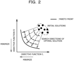
FIG. 2 is a diagram exemplifying a case where a genetic algorithm is used for a multi-objective optimization engine. -
FIG. 3 is a diagram exemplifying a linear weighted sum method. -
FIG. 4(a) is a functional block diagram representing an overall configuration of an information processing device according to a first embodiment, andFIG. 4(b) is a hardware configuration diagram of the information processing device. -
FIG. 5 is a diagram exemplifying a flowchart of the first embodiment. -
FIGs. 6(a) and 6(b) are explanatory diagrams of the first embodiment. -
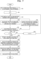
FIG. 7 is a diagram exemplifying a flowchart of a second embodiment. -
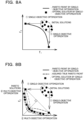
FIGs. 8(a) and 8(b) are explanatory diagrams of the second embodiment. -
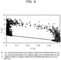
FIG. 9 is a diagram illustrating calculation results. -
FIG. 10 is a diagram illustrating calculation results. -
FIG. 11 is a diagram for describing a hypervolume. -
FIG. 12 is a diagram exemplifying a production line model. -
FIGs. 13(a) to 13(c) are diagrams exemplifying product information. -
FIG. 14 is a diagram illustrating calculation results. -
FIG. 15 is a diagram illustrating calculation results. - There are optimization problems in fields of various industries including a manufacturing industry and a distribution industry. For example, in an optimization problem of a production plan at a manufacturing field, there is a problem that a relationship between a manufacturing time needed for a certain production plan and a cost generated in proportion to an operation time of a device becomes a trade-off. For example, there is a problem of a trade-off that, when the manufacturing time is shortened, an operation time of a legacy device having a high operating cost is increased and a cost is increased, and the like.
- A multi-objective optimization problem for simultaneously optimizing a plurality of objective functions having a trade-off relationship is generally a problem of obtaining a Pareto solution. In the example described above, each of the manufacturing time needed for the certain production plan and the cost generated in proportion to the operation time of the device is the objective function. An explanatory variable is the production plan, and is, for example, an input order in which each product is input to a production process, or the like. The Pareto solution is a solution in which at least one of the plurality of objective functions is superior to those of other optional solutions.
FIG. 1 is a diagram exemplifying the Pareto solutions. InFIG. 1 , a solution of (f1, f2) = (9, 3) is not the Pareto solution since there is no superior objective function when compared with (f1, f2) = (8, 2). - In the example of
FIG. 1 , since optimization is performed so that each objective function is minimized, Pareto solutions positioned on a lower left side are obtained. A line coupling the respective Pareto solutions (arrangement of the respective Pareto solutions) is referred to as a Pareto front. A user selects an optimal solution suitable for a purpose from among the Pareto solutions obtained by multi-objective optimization calculation. Therefore, in order to give a large number of more optimal options to the user, in the multi-objective optimization calculation, it is needed to calculate a more optimal and wider Pareto front in as short a calculation time as possible. - For example, a case is conceivable where a plurality of objective functions desired to be optimized is set to an evaluation function of a multi-objective optimization engine and the multi-objective optimization calculation is performed.
FIG. 2 is a diagram exemplifying a case where a genetic algorithm is used as an example for the multi-objective optimization engine. The genetic algorithm is a method of obtaining a solution such that each objective function is minimized from an initial solution group by incorporating genetic elements. In the example ofFIG. 2 , directions such as moving from initial solutions to a left side and a lower side correspond to search directions. In such a method, it is often not possible to calculate an exact solution in a real time in a real problem having a large problem scale, and thus, it is needed to calculate a more optimal solution in a finite calculation time. - Therefore, a case is conceivable where the plurality of objective functions desired to be optimized is weighted, one evaluation function is set, and optimization calculation is performed with a single-objective optimization engine.
FIG. 3 is a diagram exemplifying a linear weighted sum method in this case. For example, an objective function f1 (x1)·w + an objective function f2(x1)·(1 - w) is obtained from the initial solution group, an objective function f1(x2)·w + an objective function f2(x2)·(1 - w) is obtained from the solutions, and an objective function f1(x3)·w + an objective function f2(x3)·(1 - w) is further obtained. The reference "w" corresponds to a weight, and is a value that satisfies 0 < w < 1. However, in such a method, it is difficult to obtain an appropriate weight for a plurality of indexes having different scales as the evaluation function. Furthermore, it is difficult to shorten a calculation time. - Therefore, in the following embodiments, an information processing device, an arithmetic method, and an arithmetic program that may shorten the calculation time will be described.
-
FIG. 4(a) is a functional block diagram representing an overall configuration of aninformation processing device 100 according to a first embodiment. Theinformation processing device 100 is a server for optimization processing, or the like. As exemplified inFIG. 4(a) , theinformation processing device 100 functions as an objectivefunction setting unit 10, anoptimization execution unit 20, an intermediateprocess recording unit 30, aresult output unit 40, and the like. -
FIG. 4(b) is a hardware configuration diagram of theinformation processing device 100. As exemplified inFIG. 4(b) , theinformation processing device 100 includes aCPU 101, aRAM 102, astorage device 103, aninput device 104, a display device 105, and the like. - The central processing unit (CPU) 101 is a central processing unit. The
CPU 101 includes one or more cores. The random access memory (RAM) 102 is a volatile memory that temporarily stores a program to be executed by theCPU 101, data to be processed by theCPU 101, and the like. Thestorage device 103 is a nonvolatile storage device. As thestorage device 103, for example, a read only memory (ROM), a solid state drive (SSD) such as a flash memory, a hard disk to be driven by a hard disk drive, or the like may be used. Thestorage device 103 stores an arithmetic program. Theinput device 104 is a device for a user to input needed information, and is a keyboard, a mouse, or the like. The display device 105 is a device that displays, on a screen, a result output from theresult output unit 40, or the like. Each unit of theinformation processing device 100 is implemented by theCPU 101 executing the arithmetic program. Note that hardware such as a dedicated circuit may be used as each unit of theinformation processing device 100. - The objective
function setting unit 10 sets a plurality of objective functions. The objectivefunction setting unit 10 may set two objective functions or may set three or more objective functions. In the present embodiment, the objectivefunction setting unit 10 sets N objective functions f1 to fN. Theoptimization execution unit 20 executes optimization such that the objective functions f1 to fN are optimized. The intermediateprocess recording unit 30 records a result in the middle of the execution of the optimization by theoptimization execution unit 20. Theresult output unit 40 outputs the result of the optimization executed by theoptimization execution unit 20. - Hereinafter, Pareto optimal solution calculation processing will be described with reference to a flowchart of
FIG. 5 and explanatory diagrams ofFIGs. 6(a) and 6(b) . Note thatFIGs. 6(a) and 6(b) are explanatory diagrams for the two objective functions f1 and f2. - First, the objective
function setting unit 10 sets the N objective functions (fn; n = 1 to N) desired to be optimized (step S1). Each objective function is, for example, a production completion time in a production process, a cost related to production, or the like. A shorter production completion time is better, and a lower cost is better. - Next, the
optimization execution unit 20 sets n to 1 (step S2). As a result, first, the objective function f1 is focused. - Next, the
optimization execution unit 20 sets an initial value of each explanatory variable with a random value (step S3). The number of initial values may be one or plural. The initial value may be input by a user using theinput device 104. - Next, the
optimization execution unit 20 calculates values of the objective functions f1 to fN according to the explanatory variable (step S4). In a case where step S4 is executed for the first time, the values of the objective functions f1 to fN are calculated from the initial value of the explanatory variable. In a case where there is a plurality of the initial values, an initial solution group as exemplified inFIG. 6(a) is generated. - Next, the intermediate
process recording unit 30 records the explanatory variable used in step S4 and the values of the objective functions f1 to fN calculated in step S4 (step S5). Therefore, the intermediateprocess recording unit 30 records the initial solution group. - Next, the
optimization execution unit 20 determines whether or not an optimal solution of the objective function fn has converged (step S6). Here, it is determined whether or not the objective function fn has reached the best value. Note that it may be determined whether or not a solution better than the initial value has been obtained. - In a case where it is determined as "No" in step S6, the
optimization execution unit 20 updates the explanatory variable so that an evaluation function is optimized by a single-objective optimization engine (step S7). Thereafter, step S4 and the subsequent steps are executed again. - In a case where it is determined as "Yes" in step S6, the
optimization execution unit 20 determines whether or not n is N or more (step S8). By execution of step S8, it may be determined whether or not single-objective optimization has been ended for all the objective functions. - In a case where it is determined as "No" in step S8, the
optimization execution unit 20 adds 1 to n to obtain n + 1 (step S9). Thereafter, step S3 and the subsequent steps are executed again. - In a case where it is determined as "Yes" in step S8, the
optimization execution unit 20 extracts Pareto solutions from all calculation results (step S10). As a result, as exemplified inFIG. 6(a) , it is possible to extract Pareto solutions obtained by performing the single-objective optimization on each objective function. Note that the extracted Pareto solutions are recorded by the intermediateprocess recording unit 30. - Next, the
optimization execution unit 20 calculates a linear weighted sum obtained by performing weighting according to arrangement of the Pareto solutions extracted in step S10 (step S11). For example, the weighting is performed in a direction perpendicular to an approximate plane approximating the arrangement of the Pareto solutions. When there are two objective functions, an approximate straight line of the Pareto solutions is used instead of the approximate plane described above. InFIG. 6(a) , the approximate straight line approximating the Pareto solutions is obtained. An approximation method is not particularly limited, but is, for example, a least squares method or the like. InFIG. 6(b) , the approximate straight line and a direction intersecting (for example, a direction perpendicular to) the approximate straight line are drawn. This direction corresponds to a search direction of a solution. - Next, the
optimization execution unit 20 executes multi-objective optimization using the objective functions f1 to fN and the linear weighted sum as the evaluation functions (step S12). The initial value of the explanatory variable in this case is the explanatory variable corresponding to the Pareto solutions extracted in step S10. - Next, the
optimization execution unit 20 calculates Pareto solutions by using an execution result of step S12 (step S13). The Pareto solutions are drawn inFIG. 6(b) . Calculation results of step S13 are output by theresult output unit 40. - As described above, each of the plurality of N objective functions fn(x) (n = 1, ..., N) desired to be optimized is set as the evaluation function of the single-objective optimization, and the optimization is performed by the single-objective optimization engine, and each optimal solution of the single-objective optimization and an explanatory variable thereof are solved. Using each optimal solution of the single-objective optimization as a starting point, the linear weighted sum obtained by weighting each objective function in the direction perpendicular to the Pareto front is set as the evaluation function, and the multi-objective optimization calculation is executed to solve the Pareto solutions. The search direction of the optimal solutions is set with the linear weighted sum while minimizing each objective function to solve the true Pareto front.
- In this method, the single-objective optimization is performed on each objective function before the multiobjective optimization. Since the multi-objective optimization is performed using the optimal solutions obtained by the single-objective optimization as the starting points, a calculation time until reaching the true Pareto front is shortened. Note that, since a calculation load of the single-objective optimization is significantly smaller than that of the multi-objective optimization, the calculation load is reduced as a result as compared with a case where the multi-objective optimization is performed without performing the single-objective optimization, and the calculation time may be shortened.
- In the first embodiment, a result of an optimal calculation process is used in the single-objective optimization, but the present invention is not limited to this. In a second embodiment, a case will be described where a result of an optimal calculation process is not used in single-objective optimization.
- Hereinafter, Pareto optimal solution calculation processing according to the second embodiment will be described with reference to a flowchart of
FIG. 7 and explanatory diagrams ofFIGs. 8(a) and 8(b) . Note thatFIGs. 8(a) and 8(b) are explanatory diagrams for two objective functions f1 and f2. - First, the objective
function setting unit 10 sets N objective functions (fn; n = 1 to N) desired to be optimized (step S21). Each objective function is, for example, a production completion time in a production process, a cost related to production, or the like. A shorter production completion time is better, and a lower cost is better. - Next, the
optimization execution unit 20 sets n to 1 (step S22). As a result, first, the objective function f1 is focused. - Next, the
optimization execution unit 20 sets an initial value of an explanatory variable with a random value (step S23). The number of initial values may be one or plural. The initial value may be input by a user using theinput device 104. - Next, the
optimization execution unit 20 calculates values of the objective functions f1 to fN according to the explanatory variable (step S24). In a case where step S24 is executed for the first time, the values of the objective functions f1 to fN are calculated from the initial value of the explanatory variable. In a case where there is a plurality of the initial values, an initial solution group as exemplified inFIG. 8(a) is generated. - Next, the
optimization execution unit 20 determines whether or not an optimal solution of the objective function fn has converged (step S25). Here, it is determined whether or not the objective function fn has reached the best value. Note that it may be determined whether or not a solution better than the initial value has been obtained. - In a case where it is determined as "No" in step S25, the
optimization execution unit 20 updates the explanatory variable so that an evaluation function is optimized by a single-objective optimization engine (step S26). Thereafter, step S24 and the subsequent steps are executed again. - In a case where it is determined as "Yes" in step S26, the
optimization execution unit 20 determines whether or not n is N or more (step S27). By execution of step S27, it may be determined whether or not the single-objective optimization has been ended for all the objective functions. - In a case where it is determined as "No" in step S27, the
optimization execution unit 20 adds 1 to n to obtain n + 1 (step S28). Thereafter, step S23 and the subsequent steps are executed again. - In a case where it is determined as "Yes" in step S27, the
optimization execution unit 20 extracts an optimal solution for each objective function (step S29). As exemplified inFIG. 8(a) , a solution having the lowest value of f1 and a solution having the lowest value of f2 are extracted as the optimal solutions. Note that each of the extracted optimal solutions is recorded by the intermediateprocess recording unit 30. - Next, the
optimization execution unit 20 calculates a linear addition sum obtained by performing weighting according to arrangement of the optimal solutions extracted in step S29 (step S30). For example, the weighting is performed in a direction perpendicular to a surface coupling the optimal solutions. When there are two objective functions, a straight line coupling the optimal solutions is used. InFIG. 8(a) , the straight line coupling the optimal solutions is obtained. InFIG. 8(b) , the line coupling the optimal solutions and a direction intersecting (for example, a direction perpendicular to) the line are drawn. This direction corresponds to a search direction of a solution. - Next, the
optimization execution unit 20 executes multi-objective optimization using the objective functions f1 to fN and the linear weighted sum as the evaluation functions (step S31). The initial value of the explanatory variable in this case is an explanatory variable corresponding to the optimal solutions extracted in step S29. - Next, the
optimization execution unit 20 calculates Pareto solutions by using an execution result of step S31 (step S32). The Pareto solutions are drawn inFIG. 8(b) . Calculation results of step S32 are output by theresult output unit 40. - As described above, each of the plurality of N objective functions fn(x) (n = 1, ..., N) desired to be optimized is set as the evaluation function of the single-objective optimization, and the optimization is performed by the single-objective optimization engine, and each optimal solution of the single-objective optimization and an explanatory variable thereof are solved. Using each optimal solution of the single-objective optimization as a starting point, each objective function fn and the linear weighted sum obtained by weighting each objective function in the direction perpendicular to a Pareto front are set as the evaluation functions, and the multi-objective optimization calculation is executed to solve the Pareto solutions. The search direction of the optimal solutions is set with the linear weighted sum while minimizing each objective function to solve the true Pareto front.
- In this method, the single-objective optimization is performed on each objective function before the multiobjective optimization. Since the multi-objective optimization is performed using the optimal solutions obtained by the single-objective optimization as the starting points, a calculation time until reaching the true Pareto front is shortened. Note that, since a calculation load of the single-objective optimization is significantly smaller than that of the multi-objective optimization, the calculation load is reduced as a result as compared with a case where the multi-objective optimization is performed without performing the single-objective optimization, and the calculation time may be shortened.
- Hereinafter, simulation results for the first embodiment will be described. As the objective functions, f1 and f2 are used. The multi-objective optimization was performed to minimize these objective functions. As an example, a standard problem of the following expression was used. This standard problem is disclosed in "Eckart Zitzler, Kalyanmoy Ded, and Lothar Thiele, Comparison of Multiobjective Evolutionary Algorithms: Empirical Results, Evolutionary Computation, vol. 8, ).".

- The following expressions are used as examples of the objective function f1 and the objective function f2.


- Here, g(x2, ..., xm) may be represented as the following expression.

- Note that it is assumed that m = 30 holds and the following expression holds.

- The single-objective optimization was performed for each of the objective functions described above. An explanatory variable x = (x1, x2, ..., x30) with an initial value set with a random value was updated by the single-objective optimization engine to minimize the objective functions. In each single-objective optimization, results of a calculation process (values of the explanatory variable x and f1(x) and f2(x)) were also output. Pareto solutions and explanatory variables thereof were obtained from all calculation results including the results of the calculation process of the single-objective optimization.
FIG. 9 is a diagram illustrating the calculation results. As illustrated in the results ofFIG. 9 , in the single-objective optimization, the results are concentrated in a region where the value of f1(x) is small and a region where the value of f2(x) is small. - Next, using the Pareto solutions of f1(x) and f2(x) as starting points, the multi-objective optimization was performed with three objective functions including a linear weighted sum weighted in a direction perpendicular to an approximate straight line of a Pareto front, f1(x), and f2(x). Results are indicated in
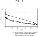
FIG. 10 . InFIG. 10 , the Pareto solutions obtained by the method ofFIG. 2 are also indicated. When the method ofFIG. 2 and the method according to the first embodiment are compared with each other at the same number of times of calculation (about 4900 times), it may be seen that a more optimal Pareto front was able to be calculated by the method according to the first embodiment. Therefore, it may be seen that the calculation time for obtaining the same Pareto front was shortened. When the comparison is performed by using a hypervolume, the hypervolume was 1.3% lower in the method according to the first embodiment than in the method according toFIG. 2 . -
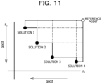
FIG. 11 is a diagram for describing the hypervolume. The hypervolume is a performance index for the Pareto solution. Specifically, the hypervolume represents an area or a volume of a region formed by a certain reference point and a solution set obtained by an algorithm in an objective function space. As an example, it is possible to use a standardized value of each objective function with the reference point of (0, 0). In a case where two objective functions are used, the area represented inFIG. 11 is the hypervolume. As the hypervolume is larger, the solution is wider, so that it may be determined that a favorable result is obtained. - Next, simulation results of the second embodiment will be described. In the second embodiment, the objective function was set using a specific layout of a manufacturing field.
-
FIG. 12 is a diagram exemplifying a production line model. As exemplified inFIG. 12 , the production line model contains branches and merges, and a plurality of products is input one by one. For each of the plurality of products, a plurality of works is performed in order. At least a part of the works are different for the plurality of products. - The production line model in
FIG. 12 is a production line model including aprocess 1 and aprocess 2. When theprocess 1 and theprocess 2 are passed through in accordance with a product input order, branching and merging are repeated, and finally shipping is carried out through inspection and packaging processes. In theprocess 1, threemanufacturing devices 1 with the same specifications are arranged. Before the work is performed in eachmanufacturing device 1, a changeover (work of changing setting of a jig or a device of a processing machine according to a type of a product to be produced) is performed. - In the
process 2, no changeover is needed. In theprocess 2, threemanufacturing devices 2 and two legacy devices with specifications different from those of themanufacturing devices 2 are arranged. The legacy device is a costly and time consuming device. - As an example, there are two changeover workers. Therefore, it is possible to simultaneously perform the changeover in at most two devices in parallel. A cost of each device increases in proportion to an operation time of the device.
- With such a layout, as an example, a plan for optimizing a manufacturing time and a cost is made. For example, when it is attempted to shorten the manufacturing time by reducing the changeover, use of the legacy device increases and the cost increases, so that the manufacturing time and the cost are in a trade-off relationship.
-
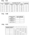
FIGs. 13(a) to 13(c) are diagrams exemplifying product information.FIG. 13(a) is a diagram exemplifying master information in a production master.FIG. 13(b) is a diagram exemplifying an operation cost in the production master.FIG. 13(c) is a diagram exemplifying a takt time of a changeover in the production master. - As exemplified in
FIG. 13(a) , the number of manufactured products, a processing takt time of themanufacturing device 1, a processing takt time of themanufacturing device 2, a processing takt time of the legacy device, and a changeover specification are associated with each of product types A to E. As exemplified inFIG. 13(b) , a device operation cost coefficient is associated with each manufacturing device. The operation cost is calculated by multiplying the processing takt time by the coefficient. As exemplified inFIG. 13(c) , a changeover takt time is associated with a combination of a subsequent product/a previous product. The previous product for a certain device is a type of a product for which a manufacturing process has been performed in the device so far. The subsequent product is a type of a product for which a manufacturing process is performed next in the device. A number of "subsequent product/previous product" is associated with a combination of the respective products. - Two objective functions were set: the manufacturing time and the cost. It was assumed that a calculation time was extremely short by using a single-objective solving specialized engine capable of high-speed solving. A random value was set as an initial value. Results are indicated in
FIG. 14 . A horizontal axis indicates the manufacturing time, and a vertical axis indicates the cost. A single-objective optimal solution is obtained for each of manufacturing time and the cost. - Next, the multi-objective optimization was performed with three objective functions of a linear weighted sum obtained by performing weighting in a direction perpendicular to a straight line coupling optimal solutions, the manufacturing time, and the cost using each single-objective optimal solution of the manufacturing time and the cost as a starting point. Results are indicated in
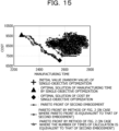
FIG. 15 . Since a result (HV = 0.576) equivalent to the Pareto front obtained by the method of the second embodiment (the number of times of calculation is about 600) may be obtained by the number of times of calculation of 1600 in the method ofFIG. 2 , it was possible to reduce a calculation amount by about 60%. Comparing the results of the method ofFIG. 2 and the method of the second embodiment with the same number of times of calculation (about 600 times), a wider optimal Pareto front (HV is about twice) was calculated. - Note that, in each of the examples described above, the genetic algorithm is used as an optimization algorithm, but the present invention is not limited to this. Other optimization algorithms such as evolutionary algorithms may be used.
- In each of the examples described above, the
optimization execution unit 20 is an example of an execution unit that calculates single-objective optimal solutions that have better values than initial solutions by executing single-objective optimization by using each of a plurality of objective functions as a first evaluation function for the initial solutions, and executes, by using the single-objective optimal solutions as starting points, multiobjective optimization for a second evaluation function by using, as the second evaluation function, a linear weighted sum obtained by performing weighting for each of the plurality of objective functions according to the single-objective optimal solutions. - While the embodiments of the present invention have been described above in detail, the present invention is not limited to such specific embodiments, and a variety of modifications and alterations may be made within the scope of the gist of the present invention described in the claims.
- All examples and conditional language provided herein are intended for the pedagogical purposes of aiding the reader in understanding the invention and the concepts contributed by the inventor to further the art, and are not to be construed as limitations to such specifically recited examples and conditions, nor does the organization of such examples in the specification relate to a showing of the superiority and inferiority of the invention. Although one or more embodiments of the present invention have been described in detail, it should be understood that the various changes, substitutions, and alterations could be made hereto without departing from the spirit and scope of the invention.
-
- 10
- Objective function setting unit
- 20
- Optimization execution unit
- 30
- Intermediate process recording unit
- 40
- Result output unit
- 100
- Information processing device
- 101
- CPU
- 102
- RAM
- 103
- Storage device
- 104
- Input device
- 105
- Display device
Claims (27)
- An arithmetic program for causing a computer to execute processing comprising:calculating single-objective optimal solutions that have better values than initial solutions by executing single-objective optimization by using each of a plurality of objective functions as a first evaluation function for the initial solutions; andexecuting, by using the single-objective optimal solutions as starting points, multi-objective optimization for a second evaluation function by using, as the second evaluation function, a linear weighted sum obtained by performing weighting for each of the plurality of objective functions according to the single-objective optimal solutions.
- The arithmetic program according to claim 1, whereinthe number of the plurality of objective functions is two, andthe computer is caused to execute processing of calculating an approximate straight line approximate to arrangement of the single-objective optimal solutions obtained by the execution of the single-objective optimization and solutions at an intermediate process, and setting the weighting in a direction that intersects the approximate straight line.
- The arithmetic program according to claim 2, wherein the direction that intersects the approximate straight line is a direction perpendicular to the approximate straight line.
- The arithmetic program according to claim 1, whereinthe number of the plurality of objective functions is two, andthe computer is caused to execute processing of setting the weighting in a direction that intersects a line that couples the single-objective optimal solutions obtained by the execution of the single-objective optimization.
- The arithmetic program according to claim 4, wherein the direction that intersects the line that couples the single-objective optimal solutions is a direction perpendicular to the line that couples the single-objective optimal solutions.
- The arithmetic program according to claim 1, whereinthe number of the plurality of objective functions is three or more, andthe computer is caused to execute processing of calculating an approximate plane approximate to arrangement of the single-objective optimal solutions obtained by the execution of the single-objective optimization and solutions at an intermediate process, and setting the weighting in a direction that intersects the approximate plane.
- The arithmetic program according to claim 6, wherein the direction that intersects the approximate plane is a direction perpendicular to the approximate plane.
- The arithmetic program according to claim 1, whereinthe number of the plurality of objective functions is three or more, andthe computer is caused to execute processing of setting the weighting in a direction that intersects a surface that couples the single-objective optimal solutions obtained by the execution of the single-objective optimization.
- The arithmetic program according to claim 8, wherein the direction that intersects the surface that couples the single-objective optimal solutions is a direction perpendicular to the surface that couples the single-objective optimal solutions.
- An arithmetic method implemented by a computer, the arithmetic method comprising:calculating single-objective optimal solutions that have better values than initial solutions by executing single-objective optimization by using each of a plurality of objective functions as a first evaluation function for the initial solutions; andexecuting, by using the single-objective optimal solutions as starting points, multi-objective optimization for a second evaluation function by using, as the second evaluation function, a linear weighted sum obtained by performing weighting for each of the plurality of objective functions according to the single-objective optimal solutions.
- The arithmetic method according to claim 10, whereinthe number of the plurality of objective functions is two, andthe computer is caused to execute processing of calculating an approximate straight line approximate to arrangement of the single-objective optimal solutions obtained by the execution of the single-objective optimization and solutions at an intermediate process, and setting the weighting in a direction that intersects the approximate straight line.
- The arithmetic method according to claim 11, wherein the direction that intersects the approximate straight line is a direction perpendicular to the approximate straight line.
- The arithmetic method according to claim 10, whereinthe number of the plurality of objective functions is two, andthe computer is caused to execute processing of setting the weighting in a direction that intersects a line that couples the single-objective optimal solutions obtained by the execution of the single-objective optimization.
- The arithmetic method according to claim 13, wherein the direction that intersects the line that couples the single-objective optimal solutions is a direction perpendicular to the line that couples the single-objective optimal solutions.
- The arithmetic method according to claim 10, whereinthe number of the plurality of objective functions is three or more, andthe computer is caused to execute processing of calculating an approximate plane approximate to arrangement of the single-objective optimal solutions obtained by the execution of the single-objective optimization and solutions at an intermediate process, and setting the weighting in a direction that intersects the approximate plane.
- The arithmetic method according to claim 15, wherein the direction that intersects the approximate plane is a direction perpendicular to the approximate plane.
- The arithmetic method according to claim 10, whereinthe number of the plurality of objective functions is three or more, andthe computer is caused to execute processing of setting the weighting in a direction that intersects a surface that couples the single-objective optimal solutions obtained by the execution of the single-objective optimization.
- The arithmetic method according to claim 17, wherein the direction that intersects the surface that couples the single-objective optimal solutions is a direction perpendicular to the surface that couples the single-objective optimal solutions.
- An information processing device comprising:an execution unit configured tocalculate single-objective optimal solutions that have better values than initial solutions by executing single-objective optimization by using each of a plurality of objective functions as a first evaluation function for the initial solutions, andexecute, by using the single-objective optimal solutions as starting points, multi-objective optimization for a second evaluation function by using, as the second evaluation function, a linear weighted sum obtained by performing weighting for each of the plurality of objective functions according to the single-objective optimal solutions.
- The information processing device according to claim 19, whereinthe number of the plurality of objective functions is two, andthe execution unit calculates an approximate straight line approximate to arrangement of the single-objective optimal solutions obtained by the execution of the single-objective optimization and solutions at an intermediate process, and sets the weighting in a direction that intersects the approximate straight line.
- The information processing device according to claim 20, wherein
the direction that intersects the approximate straight line is a direction perpendicular to the approximate straight line. - The information processing device according to claim 19, whereinthe number of the plurality of objective functions is two, andthe execution unit sets the weighting in a direction that intersects a line that couples the single-objective optimal solutions obtained by the execution of the single-objective optimization.
- The information processing device according to claim 22, wherein
the direction that intersects the line that couples the single-objective optimal solutions is a direction perpendicular to the line that couples the single-objective optimal solutions. - The information processing device according to claim 19, whereinthe number of the plurality of objective functions is three or more, andthe execution unit calculates an approximate plane approximate to arrangement of the single-objective optimal solutions obtained by the execution of the single-objective optimization and solutions at an intermediate process, and sets the weighting in a direction that intersects the approximate plane.
- The information processing device according to claim 24, wherein
the direction that intersects the approximate plane is a direction perpendicular to the approximate plane. - The information processing device according to claim 25, whereinthe number of the plurality of objective functions is three or more, andthe execution unit sets the weighting in a direction that intersects a surface that couples the single-objective optimal solutions obtained by the execution of the single-objective optimization.
- The information processing device according to claim 26, wherein
the direction that intersects the surface that couples the single-objective optimal solutions is a direction perpendicular to the surface that couples the single-objective optimal solutions.
Applications Claiming Priority (1)
| Application Number | Priority Date | Filing Date | Title |
|---|---|---|---|
| PCT/JP2022/032329 WO2024047682A1 (en) | 2022-08-29 | 2022-08-29 | Computation program, computation method, and information processing device |
Publications (2)
| Publication Number | Publication Date |
|---|---|
| EP4583025A1 true EP4583025A1 (en) | 2025-07-09 |
| EP4583025A4 EP4583025A4 (en) | 2025-10-22 |
Family
ID=90099107
Family Applications (1)
| Application Number | Title | Priority Date | Filing Date |
|---|---|---|---|
| EP22957288.8A Pending EP4583025A4 (en) | 2022-08-29 | 2022-08-29 | CALCULATION PROGRAM, CALCULATION METHOD AND INFORMATION PROCESSING DEVICE |
Country Status (4)
| Country | Link |
|---|---|
| US (1) | US20250173390A1 (en) |
| EP (1) | EP4583025A4 (en) |
| JP (1) | JP7839431B2 (en) |
| WO (1) | WO2024047682A1 (en) |
Families Citing this family (1)
| Publication number | Priority date | Publication date | Assignee | Title |
|---|---|---|---|---|
| WO2026058462A1 (en) * | 2024-09-12 | 2026-03-19 | 三菱電機株式会社 | Good solution identification device and good solution identification method |
Family Cites Families (7)
| Publication number | Priority date | Publication date | Assignee | Title |
|---|---|---|---|---|
| JP2002366587A (en) | 2001-06-07 | 2002-12-20 | Hitachi Ltd | Optimization method |
| JP5003499B2 (en) * | 2008-01-14 | 2012-08-15 | 富士通株式会社 | Multi-objective optimization design support apparatus, method, and program |
| JP5282493B2 (en) * | 2008-09-04 | 2013-09-04 | 富士通株式会社 | Optimal solution relation display device, method, and program |
| US9299032B2 (en) | 2012-11-12 | 2016-03-29 | International Business Machines Corporation | Multi objective design selection |
| US20150019173A1 (en) | 2013-07-09 | 2015-01-15 | International Business Machines Corporation | Multiobjective optimization through user interactive navigation in a design space |
| EP4123554A4 (en) * | 2020-03-17 | 2023-04-19 | Fujitsu Limited | INFORMATION PROCESSING DEVICE, WORK PLAN DETERMINATION METHOD, AND WORK PLAN DETERMINATION PROGRAM |
| JP7502975B2 (en) | 2020-11-24 | 2024-06-19 | 日鉄テックスエンジ株式会社 | Processing device, processing method, and program |
-
2022
- 2022-08-29 JP JP2024543601A patent/JP7839431B2/en active Active
- 2022-08-29 WO PCT/JP2022/032329 patent/WO2024047682A1/en not_active Ceased
- 2022-08-29 EP EP22957288.8A patent/EP4583025A4/en active Pending
-
2025
- 2025-01-29 US US19/039,792 patent/US20250173390A1/en active Pending
Also Published As
| Publication number | Publication date |
|---|---|
| JPWO2024047682A1 (en) | 2024-03-07 |
| US20250173390A1 (en) | 2025-05-29 |
| EP4583025A4 (en) | 2025-10-22 |
| WO2024047682A1 (en) | 2024-03-07 |
| JP7839431B2 (en) | 2026-04-02 |
Similar Documents
| Publication | Publication Date | Title |
|---|---|---|
| Bastani et al. | A radial basis collocation method for pricing American options under regime-switching jump-diffusion models | |
| US8249837B1 (en) | Method for optimization of sheet metal forming tool topology | |
| CN101093519A (en) | Ic layout optimization to improve yield | |
| CN113010954A (en) | Bridge structure damage identification method and device and terminal equipment | |
| JP2010061439A (en) | Optimal solution relation display apparatus, method, and program | |
| US20250173390A1 (en) | Computer-readable recording medium storing arithmetic program, arithmetic method, and information processing device | |
| CN117150603A (en) | Bridge BIM model construction system and method | |
| CN114386879B (en) | Grading and ranking method and system based on multi-product multi-dimensional performance indexes | |
| Escudero et al. | Lagrangian decomposition for large-scale two-stage stochastic mixed 0-1 problems | |
| CN116663493B (en) | Conditional constraint statement solving method, device and medium based on constraint solver | |
| JP7077667B2 (en) | Control method, control device and program | |
| Contardo | Decremental clustering for the solution of p-dispersion problems to proven optimality | |
| US20210034999A1 (en) | Optimization device, optimization method, and optimization program | |
| Kruczyk et al. | Random reducts: A monte carlo rough set-based method for feature selection in large datasets | |
| US20250342222A1 (en) | Parameter generation device, system, method, and program | |
| Gilli et al. | Solving finite difference schemes arising in trivariate option pricing | |
| US12008499B2 (en) | Information processing device, work planning method, and storage medium | |
| US20120072385A1 (en) | Technique for solving optimization problem | |
| US20240386286A1 (en) | Arithmetic method, computer-readable recording medium storing arithmetic program, and information processing device | |
| JP2022107518A (en) | Information processing system, information processing method and information processing equipment | |
| EP4575916A1 (en) | Arithmetic program, arithmetic method, and information processing device | |
| JP5817341B2 (en) | Information processing method, program, and apparatus | |
| EP4542452A1 (en) | Arithmetic program, arithmetic method, and information processing device | |
| Ross et al. | Airfoil Application of AMPL: An Automated Machine Learning Pipeline | |
| US12511447B1 (en) | Methods and systems for performing shape optimization using physics informed basis function |
Legal Events
| Date | Code | Title | Description |
|---|---|---|---|
| STAA | Information on the status of an ep patent application or granted ep patent |
Free format text: STATUS: THE INTERNATIONAL PUBLICATION HAS BEEN MADE |
|
| PUAI | Public reference made under article 153(3) epc to a published international application that has entered the european phase |
Free format text: ORIGINAL CODE: 0009012 |
|
| STAA | Information on the status of an ep patent application or granted ep patent |
Free format text: STATUS: REQUEST FOR EXAMINATION WAS MADE |
|
| 17P | Request for examination filed |
Effective date: 20250221 |
|
| AK | Designated contracting states |
Kind code of ref document: A1 Designated state(s): AL AT BE BG CH CY CZ DE DK EE ES FI FR GB GR HR HU IE IS IT LI LT LU LV MC MK MT NL NO PL PT RO RS SE SI SK SM TR |
|
| A4 | Supplementary search report drawn up and despatched |
Effective date: 20250923 |
|
| RIC1 | Information provided on ipc code assigned before grant |
Ipc: G06Q 10/0639 20230101AFI20250917BHEP Ipc: G06Q 10/04 20230101ALI20250917BHEP Ipc: G16Z 99/00 20190101ALI20250917BHEP Ipc: G06F 17/11 20060101ALI20250917BHEP Ipc: G06F 111/06 20200101ALI20250917BHEP |
|
| DAV | Request for validation of the european patent (deleted) | ||
| DAX | Request for extension of the european patent (deleted) |