EP4571099A1 - A control method for controlling a wind farm, related computer program product and electronic control device - Google Patents

A control method for controlling a wind farm, related computer program product and electronic control device Download PDF

Info

Publication number
EP4571099A1
EP4571099A1 EP23307225.5A EP23307225A EP4571099A1 EP 4571099 A1 EP4571099 A1 EP 4571099A1 EP 23307225 A EP23307225 A EP 23307225A EP 4571099 A1 EP4571099 A1 EP 4571099A1
Authority
EP
European Patent Office
Prior art keywords
wind
wind turbine
estimated
time instant
component
Prior art date
Legal status (The legal status is an assumption and is not a legal conclusion. Google has not performed a legal analysis and makes no representation as to the accuracy of the status listed.)
Pending
Application number
EP23307225.5A
Other languages
German (de)
French (fr)
Inventor
Elie KADOCHE
Florence CARTON
Cedric ENEAU
Pascal BIANCHI
Philippe Ciblat
Current Assignee (The listed assignees may be inaccurate. Google has not performed a legal analysis and makes no representation or warranty as to the accuracy of the list.)
Institut Mines Telecom IMT
TotalEnergies Onetech SAS
Original Assignee
Institut Mines Telecom IMT
TotalEnergies Onetech SAS
Priority date (The priority date is an assumption and is not a legal conclusion. Google has not performed a legal analysis and makes no representation as to the accuracy of the date listed.)
Filing date
Publication date
Application filed by Institut Mines Telecom IMT, TotalEnergies Onetech SAS filed Critical Institut Mines Telecom IMT
Priority to EP23307225.5A priority Critical patent/EP4571099A1/en
Priority to PCT/EP2024/085976 priority patent/WO2025125463A1/en
Priority to TW113148602A priority patent/TW202600965A/en
Publication of EP4571099A1 publication Critical patent/EP4571099A1/en
Pending legal-status Critical Current

Links

Images

Classifications

    • FMECHANICAL ENGINEERING; LIGHTING; HEATING; WEAPONS; BLASTING
    • F03MACHINES OR ENGINES FOR LIQUIDS; WIND, SPRING, OR WEIGHT MOTORS; PRODUCING MECHANICAL POWER OR A REACTIVE PROPULSIVE THRUST, NOT OTHERWISE PROVIDED FOR
    • F03DWIND MOTORS
    • F03D7/00Controlling wind motors 
    • F03D7/02Controlling wind motors  the wind motors having rotation axis substantially parallel to the air flow entering the rotor
    • F03D7/04Automatic control; Regulation
    • F03D7/042Automatic control; Regulation by means of an electrical or electronic controller
    • F03D7/048Automatic control; Regulation by means of an electrical or electronic controller controlling wind farms
    • F03D7/049Automatic control; Regulation by means of an electrical or electronic controller controlling wind farms in relation to the wake effect
    • FMECHANICAL ENGINEERING; LIGHTING; HEATING; WEAPONS; BLASTING
    • F03MACHINES OR ENGINES FOR LIQUIDS; WIND, SPRING, OR WEIGHT MOTORS; PRODUCING MECHANICAL POWER OR A REACTIVE PROPULSIVE THRUST, NOT OTHERWISE PROVIDED FOR
    • F03DWIND MOTORS
    • F03D7/00Controlling wind motors 
    • F03D7/02Controlling wind motors  the wind motors having rotation axis substantially parallel to the air flow entering the rotor
    • F03D7/0204Controlling wind motors  the wind motors having rotation axis substantially parallel to the air flow entering the rotor for orientation in relation to wind direction
    • FMECHANICAL ENGINEERING; LIGHTING; HEATING; WEAPONS; BLASTING
    • F03MACHINES OR ENGINES FOR LIQUIDS; WIND, SPRING, OR WEIGHT MOTORS; PRODUCING MECHANICAL POWER OR A REACTIVE PROPULSIVE THRUST, NOT OTHERWISE PROVIDED FOR
    • F03DWIND MOTORS
    • F03D7/00Controlling wind motors 
    • F03D7/02Controlling wind motors  the wind motors having rotation axis substantially parallel to the air flow entering the rotor
    • F03D7/04Automatic control; Regulation
    • F03D7/042Automatic control; Regulation by means of an electrical or electronic controller
    • F03D7/043Automatic control; Regulation by means of an electrical or electronic controller characterised by the type of control logic
    • F03D7/045Automatic control; Regulation by means of an electrical or electronic controller characterised by the type of control logic with model-based controls
    • FMECHANICAL ENGINEERING; LIGHTING; HEATING; WEAPONS; BLASTING
    • F03MACHINES OR ENGINES FOR LIQUIDS; WIND, SPRING, OR WEIGHT MOTORS; PRODUCING MECHANICAL POWER OR A REACTIVE PROPULSIVE THRUST, NOT OTHERWISE PROVIDED FOR
    • F03DWIND MOTORS
    • F03D7/00Controlling wind motors 
    • F03D7/02Controlling wind motors  the wind motors having rotation axis substantially parallel to the air flow entering the rotor
    • F03D7/04Automatic control; Regulation
    • F03D7/042Automatic control; Regulation by means of an electrical or electronic controller
    • F03D7/043Automatic control; Regulation by means of an electrical or electronic controller characterised by the type of control logic
    • F03D7/046Automatic control; Regulation by means of an electrical or electronic controller characterised by the type of control logic with learning or adaptive control, e.g. self-tuning, fuzzy logic or neural network
    • FMECHANICAL ENGINEERING; LIGHTING; HEATING; WEAPONS; BLASTING
    • F05INDEXING SCHEMES RELATING TO ENGINES OR PUMPS IN VARIOUS SUBCLASSES OF CLASSES F01-F04
    • F05BINDEXING SCHEME RELATING TO WIND, SPRING, WEIGHT, INERTIA OR LIKE MOTORS, TO MACHINES OR ENGINES FOR LIQUIDS COVERED BY SUBCLASSES F03B, F03D AND F03G
    • F05B2260/00Function
    • F05B2260/82Forecasts
    • F05B2260/821Parameter estimation or prediction
    • FMECHANICAL ENGINEERING; LIGHTING; HEATING; WEAPONS; BLASTING
    • F05INDEXING SCHEMES RELATING TO ENGINES OR PUMPS IN VARIOUS SUBCLASSES OF CLASSES F01-F04
    • F05BINDEXING SCHEME RELATING TO WIND, SPRING, WEIGHT, INERTIA OR LIKE MOTORS, TO MACHINES OR ENGINES FOR LIQUIDS COVERED BY SUBCLASSES F03B, F03D AND F03G
    • F05B2270/00Control
    • F05B2270/10Purpose of the control system
    • F05B2270/20Purpose of the control system to optimise the performance of a machine
    • FMECHANICAL ENGINEERING; LIGHTING; HEATING; WEAPONS; BLASTING
    • F05INDEXING SCHEMES RELATING TO ENGINES OR PUMPS IN VARIOUS SUBCLASSES OF CLASSES F01-F04
    • F05BINDEXING SCHEME RELATING TO WIND, SPRING, WEIGHT, INERTIA OR LIKE MOTORS, TO MACHINES OR ENGINES FOR LIQUIDS COVERED BY SUBCLASSES F03B, F03D AND F03G
    • F05B2270/00Control
    • F05B2270/30Control parameters, e.g. input parameters
    • F05B2270/32Wind speeds
    • FMECHANICAL ENGINEERING; LIGHTING; HEATING; WEAPONS; BLASTING
    • F05INDEXING SCHEMES RELATING TO ENGINES OR PUMPS IN VARIOUS SUBCLASSES OF CLASSES F01-F04
    • F05BINDEXING SCHEME RELATING TO WIND, SPRING, WEIGHT, INERTIA OR LIKE MOTORS, TO MACHINES OR ENGINES FOR LIQUIDS COVERED BY SUBCLASSES F03B, F03D AND F03G
    • F05B2270/00Control
    • F05B2270/30Control parameters, e.g. input parameters
    • F05B2270/321Wind directions
    • FMECHANICAL ENGINEERING; LIGHTING; HEATING; WEAPONS; BLASTING
    • F05INDEXING SCHEMES RELATING TO ENGINES OR PUMPS IN VARIOUS SUBCLASSES OF CLASSES F01-F04
    • F05BINDEXING SCHEME RELATING TO WIND, SPRING, WEIGHT, INERTIA OR LIKE MOTORS, TO MACHINES OR ENGINES FOR LIQUIDS COVERED BY SUBCLASSES F03B, F03D AND F03G
    • F05B2270/00Control
    • F05B2270/30Control parameters, e.g. input parameters
    • F05B2270/329Azimuth or yaw angle
    • FMECHANICAL ENGINEERING; LIGHTING; HEATING; WEAPONS; BLASTING
    • F05INDEXING SCHEMES RELATING TO ENGINES OR PUMPS IN VARIOUS SUBCLASSES OF CLASSES F01-F04
    • F05BINDEXING SCHEME RELATING TO WIND, SPRING, WEIGHT, INERTIA OR LIKE MOTORS, TO MACHINES OR ENGINES FOR LIQUIDS COVERED BY SUBCLASSES F03B, F03D AND F03G
    • F05B2270/00Control
    • F05B2270/40Type of control system
    • F05B2270/404Type of control system active, predictive, or anticipative
    • YGENERAL TAGGING OF NEW TECHNOLOGICAL DEVELOPMENTS; GENERAL TAGGING OF CROSS-SECTIONAL TECHNOLOGIES SPANNING OVER SEVERAL SECTIONS OF THE IPC; TECHNICAL SUBJECTS COVERED BY FORMER USPC CROSS-REFERENCE ART COLLECTIONS [XRACs] AND DIGESTS
    • Y02TECHNOLOGIES OR APPLICATIONS FOR MITIGATION OR ADAPTATION AGAINST CLIMATE CHANGE
    • Y02EREDUCTION OF GREENHOUSE GAS [GHG] EMISSIONS, RELATED TO ENERGY GENERATION, TRANSMISSION OR DISTRIBUTION
    • Y02E10/00Energy generation through renewable energy sources
    • Y02E10/70Wind energy
    • Y02E10/72Wind turbines with rotation axis in wind direction

Definitions

  • the present invention concerns a control method for controlling a wind farm.
  • the present invention in addition concerns a computer program product and an electronic control device configured to implement such a method.
  • the present invention concerns the domain of piloting the orientation of wind turbines within a wind farm to improve its productivity.
  • the productivity of a wind turbine i.e. the generated power, depends mainly on the velocity of the wind and its direction with respect to the wind turbine.
  • a wind turbine only produces energy if the wind reaching the wind turbine has a direction and velocity within a specific respective range.
  • the optimal wind production is reached when the wind turbine is facing the wind direction and when the wind velocity is neither too high, nor too small.
  • wind turbines are massive elements, so that the variation of their yaw angle cannot be greater than a certain threshold, e.g. few degrees by minute.
  • a certain threshold e.g. few degrees by minute.
  • the yaw actuators are always late compared the wind changes.
  • the wind turbines do not have the appropriate yaw angle, with respect to the wind direction.
  • the invention concerns a control method for controlling a wind farm a control method for controlling a wind farm comprising a plurality of wind turbines, based on a plurality of estimated general wind velocities and a plurality of estimated wind directions of the wind on the wind farm,
  • control method according to the invention comprises, for determining the rotation command at an initial time instant, optimizing a quantity depending on the power generated at further time instant, the first issue is overcome.
  • control method according to the invention makes it possible to increase the energy production of the wind farm since the control takes into consideration the local wind velocity at the contact of each wind turbine at said first time instant.
  • the second issue is thus at least partially overcome.
  • control method comprises one or more of the following features, taken solely, or according to any feasible combination:
  • the present invention also concerns a computer program product comprising instructions which, when being executed by a computer, implement such a control method.
  • the present invention also concerns an electronic control device for controlling a wind farm comprising a plurality of wind turbines, based on a plurality of estimated general wind velocities and a plurality of estimated wind directions direction of the wind on the wind farm,
  • the present invention also concerns a wind farm comprising a plurality of wind turbines and a control system, the control system comprising such an electronic control device.
  • FIG. 1 is represented a wind farm 10.
  • the wind farm 10 is for example on offshore wind farm.
  • the wind farm 10 is an onshore wind farm.
  • the wind farm 10 comprises several wind turbines 15i, for example a number N of wind turbines 15i, with "i" evolving from 0 to N-1, and a control system 20.
  • the number N is at least two, for example greater than ten, twenty, fifty or even a hundred.
  • the wind turbines 15i of the wind farm 10 are for example bottom-fixed wind turbines, i.e. wind turbines comprising a monopile solidly fixed to the ground, or to the seabed in case of offshore wind turbine.
  • the wind turbines are floating wind turbines, i.e. each wind turbine comprises a foundation floating on a water body and bearing the rest of the wind turbine.
  • the wind farm is mixed, comprising both bottom-fixed and floating wind turbines.
  • Figure 2 represents a front view of one wind turbine 15i of the wind farm 10.
  • the wind turbine 15i comprises a tower 25 extending along an elongation axis E.
  • the wind turbine 15i in addition comprises a rotor 30, for example located at an extremity of the tower 25.
  • the rotor 30 comprises blades 35 configured to rotate around a rotation axis R, which is sensibly perpendicular to the elongation axis E.
  • the blades 35 are configured to be driven in rotation around the rotation axis R, by the wind W flowing through the wind turbine 15i. Then, under the effect of wind, the blades drive the rotor in rotation around the rotation axis R, thus producing electricity.
  • the wind turbine 15i in addition comprises a yaw actuator 40 connected to the control system 20.
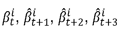
  • the yaw actuator 40 is configured, upon receiving a rotation command u t i from the control system 20 at an initial time instant t , to make the rotor 30 rotate around the elongation axis E by an angle defined in the received rotation command u t i , so that the rotor 30 reaches a desired absolute yaw angle ⁇ t + 1 i at the new time instant t + 1, in a predefined reference frame.
  • Each absolute yaw angle ⁇ t i is preferably defined as the angle formed by the rotation axis R of the wind turbine 15i, i.e. of its blade, in a predefined reference frame, for example pointing toward the cardinal points.
  • control system 20 comprises an electronic control device 45 and preferably a wind sensor 50.
  • the control device 45 is connected to each wind turbine 15 and preferably to the wind sensor 50.
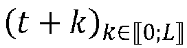
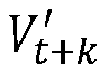
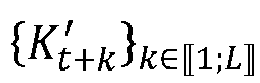
  • the optional wind sensor 50 is configured to estimate the general wind velocity V ′ t + k k ⁇ ⁇ 0 ; L ⁇ and direction K ′ t + k k ⁇ ⁇ 0 ; L ⁇ on the wind farm 10, at plurality of successive time instants t + k k ⁇ ⁇ 0 ; L ⁇ , where V t + k ' is the estimated wind velocity at time instant t + k and K t + k ' in the estimated wind direction at time instant t + k.
  • estimate is used to mean both measured and predicted.
  • L ⁇ represents a set of successive time instants comprising L + 1 time instants and starting by the initial time instant t.
  • a delay between two successive time instants is for example constant, and preferably comprised between ten seconds and twenty minutes.
  • the delay between two successive time instants is not constant.
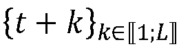
  • a k k ⁇ ⁇ 0 ; L ⁇ is the set of successive elements a k for k evolving from 0 to L. It leads that t + k k ⁇ ⁇ 0 ; L ⁇ is equivalent to the set t, t + 1, ..., t + L.
  • V ′ t + k k ⁇ ⁇ 0 ; L ⁇ is equivalent to the set V' t , V' t +1 , ..., V' t + L , and K ′ t + k k ⁇ ⁇ 0 ; L ⁇ is equivalent to the set K' t , K' t +1 , ..., K' t + L .
  • the wind sensor 50 is preferably configured to measure the general wind velocity V' t and wind direction K' t and an initial time instant t, and to predict the general wind velocity V ′ t + k k ⁇ ⁇ 0 ; L ⁇ and direction K ′ t + k k ⁇ ⁇ 0 ; L ⁇ for further time instants t + k k ⁇ ⁇ 0 ; L ⁇ , via known forecast techniques.
  • the control device 45 comprises a receiving module 55, a calculating module 60, a sending module 65 and preferably a pretreatment module 67.
  • control device 25 is a computer. It comprises a processor 70 and a memory 75 associated with the processor 70.
  • the receiving module 55, the calculating module 60, and optionally the sending module 65 and/or the pretreatment module 67 are each implemented in the form of software, or a software brick, and can be executed by the processor 70.
  • the memory 75 of the control device 45 is then able to store a receiving software, a calculating software, a sending software, and optionally a pretreatment software.
  • control device 45 When the control device 45 is implemented in the form of one or more software programs, i.e. in the form of a computer program, it can also be recorded on a computer-readable medium (not shown).
  • the computer-readable medium is, for example, a medium capable of storing electronic instructions and of being coupled to a bus of a computer system.
  • the readable medium is an optical disk, a magneto-optical disk, a ROM memory, a RAM memory, any type of non-volatile memory (e.g. EPROM, EEPROM, FLASH, NVRAM), a magnetic card or an optical card.
  • a computer program containing software instructions is stored on the readable medium.
  • the receiving module 55, the calculating module 60, the sending module 65 and optionally the pretreatment module 67 are each implemented in the form of a programmable logic component, such as an FPGA (Field Programmable Gate Array), or an integrated circuit, such as an ASIC (Application Specific Integrated Circuit).
  • a programmable logic component such as an FPGA (Field Programmable Gate Array)
  • an integrated circuit such as an ASIC (Application Specific Integrated Circuit).
  • the receiving module 55 is configured to receive, for the set of successive time instants t + k k ⁇ ⁇ 0 ; L ⁇ , the estimated wind velocities V t + k ′ k ⁇ ⁇ 0 ; L ⁇ and the estimated wind directions K ′ t + k k ⁇ ⁇ 0 ; L ⁇ of the wind W, on the wind farm 10.
  • the receiving module 55 is configured to received said estimated general wind velocities V t + k ′ k ⁇ ⁇ 0 ; L ⁇ and directions K t + k ′ k ⁇ ⁇ 0 ; L ⁇ , from the wind sensor 50.
  • the receiving module 55 is configured to receive said wind velocities V t + k ′ k ⁇ ⁇ 0 ; L ⁇ and directions V t + k ′ k ⁇ ⁇ 0 ; L ⁇ , from an external device, not represented, for example a general weather forecasting system excluded from the control system 20.
  • the receiving module 55 is configured to receive the absolute yaw angle ⁇ t i of each wind turbine 15i at said first time instant t.
  • the receiving module 55 is configured to receive each absolute yaw angle ⁇ t i from the respective yaw actuator 40, and/or to keep it in its memory 75.
  • the calculating module 60 is configured to determine, at said first time instant t and for each wind turbine 15i, a respective rotation command u t i , from the estimated wind directions K t + k ′ k ⁇ ⁇ 0 ; L ⁇ and estimated general wind velocities of the wind V t + k ′ k ⁇ ⁇ 0 ; L ⁇ on the wind farm 10, by solving an optimization problem.
  • the optimization problem aims at maximizing a power quantity f obj representative of a power generated by the wind farm 10 for said set of successive time instants t + k k ⁇ ⁇ 0 ; L ⁇ , the power quantity f obj comprising a first component C 1 and a second component C 2.
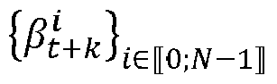
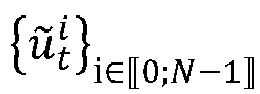
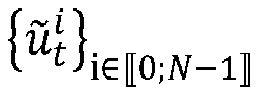
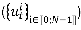
  • the first component C 1 depends on local wind velocities v t i ′ i ⁇ ⁇ 0 ; N ⁇ 1 ⁇ at the contact of each wind turbine 15i at said first time instant t , which is estimated from the rotation commands u t i i ⁇ ⁇ 0 ; N ⁇ 1 ⁇ of each wind turbine 15i at said first time instant t .
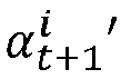
  • the first component C 1 in addition depends on the relative yaw angles ⁇ t + 1 i ′ i ⁇ ⁇ 0 ; N ⁇ 1 ⁇ between the rotation axis R of each wind turbine 15i and the wind direction K' t at the time instant t + 1 next to the initial time instant t, wherein each relative yaw angle ⁇ t + 1 i ′ is determined based on the rotation command u t i of the considered wind turbine 15i at said first time instant t .
  • the wind direction K t ′ is defined as the angle between a mean orientation the wind W between time instants t and t + 1, and a predefined frame, the frame for example pointing toward the cardinal points.
  • each relative yaw angle ⁇ t + 1 i ′ depends on the corresponding absolute yaw angle ⁇ t + 1 i and the general wind direction K t ′ .
  • each absolute yaw angle ⁇ t + 1 i at the next time instant t + 1 depends on the corresponding rotation command u t i at the initial time instant t.
  • each relative yaw angle ⁇ t + 1 i ′ depends on said rotation command u t i .
  • the first component C 1 comprises a first contribution C 1 i for each wind turbine 15i.
  • Each first contribution C 1 i is equal to zero if the respective relative yaw angle ⁇ t + 1 i ′ between each wind turbine 15i and the wind direction K' t is lower than a cut-in angle value ⁇ cut-in or higher than a cut-out angle value ⁇ 'cut-out .
  • each first contribution C 1 i is equal to the product of a first factor F 1 i , and the indicator function , the first factor F 1 i depending on the local wind velocity v t i ′ .
  • the air density ⁇ , the rotor blade area A and the power coefficient C p are preferably predefined.
  • the power coefficient C p preferably defines a cut-in velocity value v cut-in and a cut-out velocity value v cut-out .
  • the wind turbine 15i does not output power since said velocity is not high enough to drive the blades.
  • the local wind velocity v t i ′ is higher than the cut-out velocity value v cut-out , the power generated reaches a threshold and remains constant.
  • FIG. 4 An example of a theoretical power curve is shown in Figure 4 representing the evolution of the theoretical power ⁇ as a function of the local wind velocity v t i ′ for a wind turbine 15i perfectly facing the wind W .
  • the first contribution C 1 i is preferably equal to where f power is the function associating to a couple of local velocity v t i ′ and relative yaw angle ⁇ t + 1 i ′ , and estimation of the power output from the wind turbine 15i.
  • the first component C 1 is thus preferably equal to the sum of the first contribution C 1 i of each wind turbine 15i, normalized by the number of wind turbines 15i, i.e. according to the following equation:
  • v t i ′ One way to determine the local wind velocities v t i ′ is to proceed to a simulation of the wind flowing around the wind turbines 15i between time instants t and t + 1.
  • the simulation is performed via the open-source tool FLORIS (FLOw Redirection and Induction in Steady state), known per se.
  • FLORIS FLLOw Redirection and Induction in Steady state
  • the MPC problem is strongly complex since it takes into consideration, for each time instant t + k k ⁇ ⁇ 0 ; L ⁇ , and for each wind turbine 15i, the corresponding local wind velocity v t + k i ′ .
  • said local wind velocities v t + k i ′ k ⁇ ⁇ 0 ; L ⁇ , i ⁇ ⁇ 0 ; N ⁇ 1 ⁇ depends on the wake effect, i.e. on the influence of other wind turbines 15i at preceding time instants.
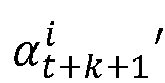
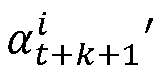
  • the wake effect at said time instant t + k depends on the relative yaw angles ⁇ t + k + 1 i ′ i ⁇ ⁇ 0 ; N ⁇ 2 ⁇ of each wind turbines 15i, at the next time instant t + k + 1, i.e. on both the absolute yaw angles ⁇ t + k i i ⁇ ⁇ 0 ; N ⁇ 1 ⁇ and the rotation commands u t + k i i ⁇ ⁇ 0 ; N ⁇ 1 ⁇ at said time instant t + k, cf equations [1] and [2].
  • each absolute yaw angle ⁇ t + k i depends on the rotation commands u t + k ⁇ 1 i at the preceding time instant, cf equation [1]. It leads that, determining the local wind velocities v t + k i i ⁇ ⁇ 0 ; N ⁇ 1 ⁇ for time instants t + k, further than time instant t + 1, is strongly complex and requires a lot of simulations.
  • the second component C 2 is simplified compared to the optimal second component C 2* so that the second component C 2 depends on a calculated rotation command u ⁇ t + k i k ⁇ ⁇ 1 ; L ⁇ for the wind turbines (15i) to rotate toward the estimated wind directions K t + k ′ k ⁇ ⁇ 1 ; L ⁇ for each further time instant t + k k ⁇ ⁇ 1 ; L ⁇ .
  • Such calculated rotation command u ⁇ t + k i is obtained by any controller able to determine analytically rotation commands from the other parameters. It is understood by "analytically”, that it exists a formula for determining such command without any optimization.
  • clip is the function determining each calculated rotation command u ⁇ t + k i , as:
  • the second component C 2 comprises, for each further time instant t + k k ⁇ ⁇ 1 ; L ⁇ , a temporal variable C 2 t + k .
  • Each temporal variable C 2 t + k comprises a second contribution C 2 t + k i for each wind turbine 15i.
  • Each second contribution C 2 t + k i i ⁇ ⁇ 0 ; N ⁇ 1 ⁇ depends on an expected relative yaw angle ⁇ ⁇ t + k + 1 i ′ between the wind turbine 15i and the wind direction K' t + k , considering that the wind turbine 15i implemented the calculated rotation command u ⁇ t + k i .
  • each relative yaw angle ⁇ t + k + 1 i ′ is replaced by the expected relative yaw angle ⁇ ⁇ t + k + 1 i ′ if the naive controller was used instead. It reduces the complexity coming from the optimization, as the naive controller provide an explicit solution, i.e. a calculated rotation command u ⁇ t + k i without requiring solving an optimization problem but directly from a formula, as show in equation [12].
  • the cosine function at power p of each relative yaw angle ⁇ t + k + 1 i ′ is replaced with a simpler penalization for relative yaw misalignment.
  • the indicator function is removed so that there is no discontinuity. Even if an expected relative yaw angle ⁇ ⁇ t + k + 1 i is too great, it can be of some interest for the optimization to know about the potential power output. The more a wind turbine 15i is misaligned, the less likely it will be to produce energy and the more it will be penalized.
  • each temporal variable C 2 t + k comprises a factor ⁇ k -1 , denoted discount factor ⁇ k -1 , making decrease the influence, on the second component C 2, of temporal variable C 2 t + k as a function of the further time instants t + k k ⁇ ⁇ 1 ; L ⁇ remoting from the initial time instant t. It gives more importance to temporal variables C 2 t + k closed to the initial time instant t than to the temporal variables C 2 t + k remote from the initial time instant t.
  • the discount factor ⁇ k -1 is formed by considering a predefined value ⁇ at the power of: k minus 1.
  • the predefined value ⁇ is comprised between 0 and 1.
  • each local wind velocity v t + k i ′ is replaced by any wind velocity which does not depend on any simulation process.
  • each local wind velocity v t + k i ′ is replaced by the estimated general wind velocity V' t + k .
  • This approximation corresponds to considering that for further time instants t + k, the wind W is received by each wind turbine 15i with the general wind velocity V t + k ′ thus neglecting the wake effect for further time instants t + k. It reduces the complexity coming from the simulation since it is not require to use a simulation for time instants further than the initial time instant t .
  • the second component C 2 forms an heuristic of the first component C 1.
  • this heuristic C 2 depends on neither the future optimized yaw settings (naive control), nor the future local velocities (no simulation), it does not increase complexity.
  • the heuristic C 2 is a scalar acting as a penalization for the optimization.
  • each calculated rotation command u ⁇ t + k i is open-loop determined, i.e. determined only based on the parameter of the heuristic C 2 without requiring any optimization process.
  • the heuristic C 2 is the discounted, weighted sum of the future theoretical power outputs.
  • the heuristic C 2 evaluates how well the wind turbines 15i will manage to stay aligned with the each estimated wind direction K' t + k .
  • the calculating module 60 is configured to solve is the simplified optimization problem of equation [18].
  • an advantage of the simplified optimization problem compared to the MPC problem is that it considerably reduces the amount of parameter to optimize by only optimizing the rotation commands u t i at the initial time instant t.
  • the calculated rotation commands u ⁇ t + k i k ⁇ ⁇ 1 ; L ⁇ , i ⁇ ⁇ 0 ; N ⁇ 1 ⁇ are open-loop determined, i.e. it exists a formula determining each calculated rotation command u ⁇ t + k i from the other parameters of the simplified optimization problem, without requiring performing any optimization.
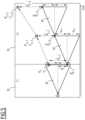
  • the x-axis represents the succession of time instants t + k k ⁇ ⁇ 0 ; 3 ⁇ .
  • the abscissa axis represents four time instants t, t + 1, t + 2, t + 3.
  • the y-axis corresponds to yaw angles ⁇ t i , ⁇ ⁇ t + 1 i , ⁇ ⁇ t + 2 i , ⁇ ⁇ t + 3 i and wind directions K' t , K' t +1 , K' t +2 , K' t +3 of a chosen wind turbine 15i.
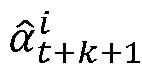
  • the crosses corresponds to the absolute yaw angles ⁇ t i , ⁇ ⁇ t + 1 i , ⁇ ⁇ t + 2 i , ⁇ ⁇ t + 3 i at the successive time instants t + k k ⁇ ⁇ 0 ; 3 ⁇ .
  • a distance between said projection and the corresponding cross i.e. the actual value of the absolute yaw angle ⁇ ⁇ t + k + 1 i , is the rotation command u t + k i , or calculated rotation command u ⁇ t + k i at the preceding time instant.
  • the triangles 80 formed from each cross and extending until the next time instant correspond to the range of rotation command u t + k i that are feasible for the next time instant, such that the absolute yaw angle ⁇ ⁇ t + k + 1 i at the next time instant t + k + 1 is comprised between ⁇ ⁇ t + k i + u min and ⁇ ⁇ t + k i + u max .
  • the limits of said triangle 80 are defined by the lower u min and upper u m ⁇ x bounds.
  • the circles corresponds to the estimated wind direction K ′ t + k k ⁇ ⁇ 0 ; 3 ⁇ at each time instant t + k k ⁇ ⁇ 0 ; 3 ⁇ .
  • the distance between the cross and the circle corresponds to the relative yaw angle ⁇ t + k i ′ at said time instant t + k.
  • Figure 5 is divided into a first part 85 and a second part 90.
  • the first part 85 corresponds to the first component C1 and the second part 90 corresponds to the second component C 2 of the power quantity f obj .
  • the first part 85 only corresponds to the initial time instant t and the incidence, on the next time instant t + 1, of the rotation command u t i determined at said time instant t.
  • the determination said rotation command u t i results from the optimization of the first component C1 as it is described below. Thus a real optimization is performed on the first part 85.
  • the second part 90 corresponds to the further time instants t + k k ⁇ ⁇ 1 ; 3 ⁇ and the expected absolute yaw angles ⁇ ⁇ t + k i k ⁇ ⁇ 1 ; 3 ⁇ induced by the calculated rotation commands u ⁇ t + k i k ⁇ ⁇ 1 ; 3 ⁇ determined by a naive controller.
  • the calculated rotation commands u ⁇ t + k i k ⁇ ⁇ 1 ; 3 ⁇ are determined to reduce as much as possible, for each next time instant t + k + 1, the expected relative yaw angles ⁇ ⁇ t + k + 1 i .
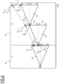
  • Figure 6 is the same figure as Figure 5 except that rotation command u t i at the initial time instant t is distinct as for Figure 5 .
  • the heuristic C 2 uses a naive controller over a future time horizon of L time instants t + k to evaluate how well the wind turbines 15i will manage to stay aligned with the predicted wind directions K t + k '.
  • the heuristic C 2 will encourage a rotation commands u t i that will put the wind turbines 15i in good orientations for the future.
  • the heuristic C 2 will penalize the first component C 1 for rotation commands u t i that would prevent wind turbines 15i from keeping track of the wind direction K t + k '.
  • the calculating module 60 is preferably configured to obtain, for each wind turbine 15i, one rotation command candidate u ⁇ t i , denoted candidate u ⁇ t i , forming a set of candidates u ⁇ t i i ⁇ ⁇ 0 ; N ⁇ 1 ⁇ comprising a respective candidate u ⁇ t i for each wind turbines 15i .
  • the calculating module 60 is then configured to determine, the corresponding local velocity v t i ′ , from:
  • the calculating module 60 is for example configured to implement equations [1], [2] and [8]. In that case, the calculating module 60 is, by the way, configured to determine corresponding relative yaw angles ⁇ t + 1 i ′ , preferably based on equation [2].
  • the calculating module 60 is configured to then calculate the first component C 1, from each corresponding local velocity v t i , and preferably from the corresponding relative yaw angles ⁇ t + 1 i ′ .
  • the calculating module 60 is in addition configured to determine, for each further time instant t + k, the corresponding calculated rotation command u ⁇ t + k i i ⁇ ⁇ 0 ; N ⁇ 1 ⁇ from the estimated wind direction K t + k ′ at said time instant t + k.
  • the calculating module 60 is configured to implement equation [12]. In that case, the calculating module 60 is configured to determine each corresponding calculated rotation command u ⁇ t + k i in addition from the expected absolute yaw angle ⁇ ⁇ t + k i determined for the previous time instant t + k - 1. For each wind turbine 15i, the expected absolute yaw angle ⁇ ⁇ t + 1 i at the time instant t + 1 is preferably equal to the absolute yaw angle ⁇ t + 1 i at said time instant t + 1, i.e. determined based on equation [1].
  • the calculating module 60 is further configured to calculate the corresponding second component C 2 from the corresponding calculated rotation commands u ⁇ t + k i , for example by implementing equation [16].
  • the calculating module 60 is configured to then calculate the corresponding power quantity f obj from the first C 1 and second C 2 components.
  • the calculating module 60 is thus configured to iterate the preceding determinations and calculations for a plurality of rotation command candidate sets u ⁇ t i i ⁇ ⁇ 0 ; N ⁇ 1 ⁇ .
  • the calculating module 60 is configured to then select the rotation commands u t i i ⁇ ⁇ 0 ; N ⁇ 1 ⁇ as the set of rotation command candidate u ⁇ t i i ⁇ ⁇ 0 ; N ⁇ 1 ⁇ , maximizing the power quantity f obj .
  • the sending module 65 is configured to send each rotation command u t i determined by the calculating module 60, to the corresponding wind turbine 15i, and in particular to its yaw actuator, so that said yaw actuator implement the received rotation command.
  • the optional pretreatment module 67 is configured apply a treatment on the estimated wind directions K t + k ′ k ⁇ ⁇ 0 ; L ⁇ on the wind farm to obtain treated wind directions K ⁇ t + k ′ k ⁇ ⁇ 0 ; L ⁇ .
  • the treatment is a low-pass filtering. This makes it possible to smooth the estimated wind directions K t + k ′ k ⁇ ⁇ 0 ; L ⁇ .
  • the calculating module 60 is configured to perform its solving by using the treated wind directions K ⁇ t + k ′ k ⁇ ⁇ 0 ; L ⁇ instead of the estimated wind directions K t + k ′ k ⁇ ⁇ 0 ; L ⁇ .
  • control method 100 The functioning of wind farm 10 and in particular of the control system 20 will now be detailed by a control method 100 and in reference to figure 7 representing a flowchart of said control method 100.
  • each wind turbines 15i has an absolute yaw angle ⁇ t i .
  • the general wind velocities V t + k ′ k ⁇ ⁇ 0 ; L ⁇ and wind directions K t + k ′ k ⁇ ⁇ 0 ; L ⁇ are estimated for each time instant t + k k ⁇ ⁇ 0 ; L ⁇ over an horizon L, as previously described, preferably by the sensor 50.
  • the method 100 comprises a receiving step 110, during which the electronic control device 45 receives, for the set of successive time instants t + k k ⁇ ⁇ 0 ; L ⁇ , the estimated general wind velocities V t + k ′ k ⁇ ⁇ 0 ; L ⁇ and the estimated wind directions K t + k ′ k ⁇ ⁇ 0 ; L ⁇ of the wind W , on the wind farm 10.
  • the electronic control device 45 in addition receives the absolute yaw angle ⁇ t i of each wind turbine 15i.
  • the method comprises a pretreatment step 115, wherein the electronic control device 45 apply a treatment on the estimated wind directions K t + k ′ k ⁇ ⁇ 0 ; L ⁇ on the wind farm to obtain treated wind directions K ⁇ t + k ′ k ⁇ ⁇ 0 ; L ⁇ .
  • the treatment is a low-pass filtering.
  • the method 100 then comprises a determining step 120, during which the electronic control device 45 determined, for each wind turbine 15i, the respective rotation command u t i from the set of estimated wind direction K t + k ′ k ⁇ ⁇ 0 ; L ⁇ and the set of velocity of the wind V t + k ′ k ⁇ ⁇ 0 ; L ⁇ on the wind farm 10, by solving an optimization problem as previously described.
  • the optimization problem aims at maximizing the power quantity f obj representative of a power generated by the wind farm 10 for said set of successive time instants t + k k ⁇ ⁇ 0 ; L ⁇ , the power quantity f obj comprising a first component C 1 and a second component C 2.
  • the first component C 1 depends on the local wind velocity ⁇ t i ′ at the contact of each wind turbine 15i at said initial time instant t , each local wind velocity ⁇ t i ′ depending on the rotation command u t i of each wind turbine 15i at said initial time instant t.
  • the second component C 2 depends on a set of calculated rotation command u ⁇ t + k i k ⁇ ⁇ 1 ; L ⁇ , i ⁇ ⁇ 1 ; N ⁇ 1 ⁇ for the wind turbines 15i to rotate toward the estimated wind directions K t + k ′ k ⁇ ⁇ 1 ; L ⁇ for each further time instant t + k k ⁇ ⁇ 1 ; L ⁇ .
  • control method 100 comprises the pretreatment step 115, during the determining step 120, the treated wind directions K ⁇ t + k ′ k ⁇ ⁇ 0 ; L ⁇ are used instead of the estimated wind directions K t + k ′ k ⁇ ⁇ 0 ; L ⁇
  • said optimization problem is the simplified optimization problem of the set of equations [18].
  • the determining step 120 preferably comprises an obtaining sub step 122, wherein, the electronic control device 45 obtains for each wind turbine 15i, a respective rotation command candidate u ⁇ t i , forming the set of rotation command candidates u ⁇ t i i ⁇ ⁇ 0 ; N ⁇ 1 ⁇ for the wind farm 10, .
  • the set of rotation command candidates u ⁇ t i i ⁇ ⁇ 0 ; N ⁇ 1 ⁇ is preferably provided by gridding, for each wind turbine 15i, the space between the lower bound u min and the upper bound u max , by a predefined number of points.
  • the determining step 120 then comprises a first determining sub step 124, wherein the electronic control device 45 determines the first component C 1 from each local wind velocity ⁇ t i ′ which depends on the set of obtained rotation command candidates u ⁇ t i i ⁇ ⁇ 0 ; N ⁇ 1 ⁇ .
  • each local wind velocity ⁇ t i ′ is determined by performing a simulation of the wind W flowing in the wind farm, for example based on equation [8].
  • the first component C 1 is determined based on equation [7].
  • the determining step 120 then comprises a second determining sub step 126 wherein the electronic control device 45 determines the first component C 2 from the calculated rotation commands u ⁇ t + k i i ⁇ ⁇ 0 ; N ⁇ 1 ⁇ , k ⁇ ⁇ 1 ; L ⁇ .
  • the calculated rotation command u ⁇ t + k i i ⁇ ⁇ 0 ; N ⁇ 1 ⁇ , k ⁇ ⁇ 1 ; L ⁇ are the command aiming at making the wind turbines 15i tracking the estimated wind directions K t + k ′ k ⁇ ⁇ 1 ; L ⁇ for each further time instant t + k k ⁇ ⁇ 1 ; L ⁇ .
  • the calculated rotation command u ⁇ t + k i i ⁇ ⁇ 0 ; N ⁇ 1 ⁇ , k ⁇ ⁇ 1 ; L ⁇ are determined from the estimated wind directions K t + k ′ k ⁇ ⁇ 1 ; L ⁇ and indirectly from the candidates u ⁇ t i i ⁇ ⁇ 0 ; N ⁇ 1 ⁇ , for example based on equations [12] and [1].
  • the second component C 2 is determined based on equation [16].
  • the determining step 120 further comprises a calculating sub step 128, wherein the electronic control device 45 calculates the power quantity f obj from the first C 1 and second C2 components, preferably by summing said components C 1 , C 2 .
  • said obtaining 122, determining 124, 126 and calculating 126 sub steps are iterated from a plurality of rotation command candidate sets u ⁇ t i i ⁇ ⁇ 0 ; N ⁇ 1 ⁇ , thus leading to a respective power quantity f obj for each set u ⁇ t i i ⁇ ⁇ 0 ; N ⁇ 1 ⁇ .
  • the new candidate set is preferably also obtained from the aforementioned gridding.
  • the determining step 120 then comprises a selecting sub step 129, wherein the rotation commands u t i i ⁇ ⁇ 0 ; N ⁇ 1 ⁇ are selected as the set of rotation command candidate u ⁇ t i i ⁇ ⁇ 0 ; N ⁇ 1 ⁇ , maximizing the power quantity f obj .
  • the control method 100 then comprises a sending step 130, wherein the electronic control device 45 send the determined rotation command u t i to each respective wind turbine 15i for the rotation of each wind turbine 15i.
  • the steps of the control method 100 are then iterated for the next time instant t + 1.
  • the initial time instant is the next time instant t + 1 of the preceding iteration.
  • the plurality of successive time instants extends from t + 1 until t + L + 1 so that the horizon, i.e. the number of time instants minus 1, remains equal to L.

Landscapes

  • Engineering & Computer Science (AREA)
  • Mechanical Engineering (AREA)
  • Sustainable Development (AREA)
  • Sustainable Energy (AREA)
  • Chemical & Material Sciences (AREA)
  • Combustion & Propulsion (AREA)
  • Life Sciences & Earth Sciences (AREA)
  • General Engineering & Computer Science (AREA)
  • Physics & Mathematics (AREA)
  • Artificial Intelligence (AREA)
  • Evolutionary Computation (AREA)
  • Fuzzy Systems (AREA)
  • Mathematical Physics (AREA)
  • Software Systems (AREA)
  • Wind Motors (AREA)

Abstract

The present invention concerns a control method for controlling a wind farm (10) comprising a plurality of wind turbines (15i).The control method comprises a receiving, for successive time instants, estimated general wind velocities and estimated wind directions of wind (W), on the wind farm.The control method comprises determining, for an initial time instant, rotation commands by solving an optimization problem. The optimization problem aims at maximizing a power quantity representative of power generated by the wind farm, which comprises a first component and a second component,The first component depends on a local wind velocity at the contact of each wind turbine at an initial time instant. The second component depends on a set of calculated rotation commands for the wind turbines to rotate toward the estimated wind directions for each further time instant.The control method comprises sending the determined rotation command to each respective wind turbine.

Description

  • The present invention concerns a control method for controlling a wind farm.
  • The present invention in addition concerns a computer program product and an electronic control device configured to implement such a method.
  • The present invention concerns the domain of piloting the orientation of wind turbines within a wind farm to improve its productivity.
  • The productivity of a wind turbine, i.e. the generated power, depends mainly on the velocity of the wind and its direction with respect to the wind turbine.
  • In particular, a wind turbine only produces energy if the wind reaching the wind turbine has a direction and velocity within a specific respective range. In particular, it is known the optimal wind production is reached when the wind turbine is facing the wind direction and when the wind velocity is neither too high, nor too small.
  • However, the wind reaching the wind turbine does not always have the same direction and velocity.
  • Thus, to improve the production of the wind turbine, it is known to control its yaw angle, i.e. its rotation along an elongation axis of the wind turbine, via a yaw actuator, to try to reach an optimal velocity and direction of the wind on blades of the wind turbine.
  • When considering a farm of wind turbines, it is known to measure the wind velocity and direction at a point close to the wind farm. From this measurement, it is known apply a control technique, at each time instant, consisting in commanding the yaw angle of each turbine to have each wind turbine tracking said measured wind direction.
  • However, this techniques faces two mains issues that make it strongly suboptimal.
  • Firstly, wind turbines are massive elements, so that the variation of their yaw angle cannot be greater than a certain threshold, e.g. few degrees by minute. Thus, if the wind direction is changing rapidly, it is not possible for the wind turbine to track such changes properly. In other words, in this case, the yaw actuators are always late compared the wind changes. Thus, at each time, the wind turbines do not have the appropriate yaw angle, with respect to the wind direction.
  • Secondly, such control technique does not consider the wake effect of the wind turbines. Actually, in a wind farm, when wind flows through a first wind turbine, the wind loses energy by driving the blades of the first turbines, inducing a wind velocity decrease. Such decrease depends on the yaw orientation of the first wind turbine and on the direction and velocity of the wind facing said first wind turbine. Thus, a second wind turbine receiving the wind influenced by the first wind turbine, i.e. its local wind, would not have the same optimal yaw inclination as the first wind turbine.
  • Due to the two previously presented issues, said control technique, consisting in trying to track the direction of the wind on the wind farm, leads to a suboptimal energy production of the wind farm.
  • It thus exists a need for a better control method improving the energy production of the wind farm.
  • To this end, the invention concerns a control method for controlling a wind farm a control method for controlling a wind farm comprising a plurality of wind turbines, based on a plurality of estimated general wind velocities and a plurality of estimated wind directions of the wind on the wind farm,
    • each wind turbine being configured, upon receiving a rotation command, to rotate, around an elongation axis respective of the wind turbine, according to said rotation command,
    • the method being implemented by an electronic control device and comprising the following steps at an initial time instant:
      • receiving, for a set of successive time instants, estimated general wind velocities and estimated wind directions of wind, on the wind farm, each estimated general wind velocity and each estimated wind direction being associated to a respective time instant;
      • for said initial time instant, determining, for each wind turbine, a respective rotation command from the set of estimated wind directions and the set of velocities of the wind on the wind farm, by solving an optimization problem,
    • the optimization problem aiming at maximizing a power quantity representative of a power generated by the wind farm for said set of successive time instants, the power quantity comprising a first component and a second component,
    • the first component depending on a local wind velocity at the contact of each wind turbine at said initial time instant, each local wind velocity depending on the rotation command of each wind turbine at said initial time instant,
    • the second component depending on a set of calculated rotation commands for the wind turbines to rotate toward the estimated wind directions for each further time instant,
      • sending the determined rotation command to each respective wind turbine for the rotation of each wind turbine.
  • Since the control method according to the invention comprises, for determining the rotation command at an initial time instant, optimizing a quantity depending on the power generated at further time instant, the first issue is overcome.
  • In addition, the control method according to the invention makes it possible to increase the energy production of the wind farm since the control takes into consideration the local wind velocity at the contact of each wind turbine at said first time instant. The second issue is thus at least partially overcome.
  • According to specific embodiment of the invention, the control method comprises one or more of the following features, taken solely, or according to any feasible combination:
    • each local wind velocity is obtained by simulating the influence of each wind turbine on the wind reaching the other wind turbines;
    • each rotation command is comprised between a lower bound and an upper bound;
    • the receiving, determining and sending steps are iterated several times;
    • the first component further depends on the relative yaw angle between a blade's rotation axis of each wind turbine and the wind direction,
      each relative yaw angle being determined based on the rotation command of the considered wind turbine at said initial time instant;
    • the first component comprises a first contribution for each wind turbine,
      • each first contribution being equal to zero if the respective relative yaw angle between a blade's rotation axis of each wind turbine and the wind direction is lower than a cut-in angle value or higher than a cut-out angle value,
      • each first contribution depending on the local wind velocity and the relative yaw angle, if said relative yaw angle is comprised between the cut-in angle value and the cut-out angle value;
    • the first component is equal to:
      Figure imgb0001
      wherein:
      • Φ ν t i
        Figure imgb0002
        is the theoretical power output from a wind turbine facing a wind with a local wind velocity vi',
      • cos p α t + 1 i
        Figure imgb0003
        is the cosine of the relative yaw angle at the power of p, representing the influence of a misalignement between the wind turbine (15i) and the wind direction,
      • Figure imgb0004
        is the indicator function equal to 1 if the relative yaw angle is comprised between the cut-in and cut-out angle values, and 0 else case, and N is the number of wind turbines in the wind farm;
    • the second component comprises, for each further time instant, a temporal variable,
      each temporal variable comprising a second contribution for each wind turbine, each second contribution depending on an expected relative yaw angle between the wind turbine and the wind direction, considering that the wind turbine implemented the calculated rotation command;
    • each temporal variable comprises a factor making decrease the influence, on the second component, of temporal variable as a function of the further time instants remoting from the initial time instant;
    • the second component is equal to C 2 = k = 1 L γ k 1 Φ V t + k 1 1 N 1 180 i = 0 N 1 α ^ t + k + 1 i
      Figure imgb0005
      wherein:
      • y is a predefined value defining the factor (γ k-1),
      • Φ(V' t+k ) is the theoretical power output from a wind turbine facing a wind with a general wind velocity equal to V t + k
        Figure imgb0006
        ,
      • α ^ t + k + 1 i
        Figure imgb0007
        is the expected relative yaw angle at a further time instant t + k + 1,
      • L is the number of considered time instants, and
      • N is the number of wind turbines in the wind farm;
    • at each further time instant, each calculated rotation command is determined:
      • ∘ by aligning the wind turbine toward the wind direction if said calculated rotation command is comprised between a lower bound and an upper bound, or
      • ∘ by selecting, among the lower bound and the upper bound, the one minimizing the expected relative yaw angle else case;
    • the step of determining the rotation commands, comprises the following sub steps:
      • ∘ obtaining, for each wind turbine, a respective rotation command candidate, forming a set of rotation command candidates for the wind farm,
      • ∘ determining the first component by:
        • + determining, for each wind turbine, the local wind velocity of said wind turbine, from the estimated wind direction at the initial time instant, from the estimated general velocity of the wind at the initial time instant, and from the set of rotation command candidates,
        • + calculating the first component from each local wind velocity,
      • ∘ determining the second component by:
        • + for each other further time instants, determining the calculated rotation command from the estimated wind direction at said time instant further,
        • + calculating the second component from each calculated rotation commands, and
      • ∘ calculating the power quantity from the first and second components,
        the sub steps of obtaining, determining and calculating being iterated for a plurality of rotation command candidates sets,
        the step of determining the rotation command in addition comprising the sub step of selecting the rotation commands as the set of rotation command candidate, maximizing the power quantity; and
    • the control method comprises between the receiving step and the determining step, a pretreatment step, wherein a treatment is applied on the estimated wind directions on the wind farm to obtain treated wind directions,
      • the determining step using the treated wind directions instead of the estimated wind directions,
      • preferably, the treatment being a low-pass filtering;
  • The present invention also concerns a computer program product comprising instructions which, when being executed by a computer, implement such a control method.
  • The present invention also concerns an electronic control device for controlling a wind farm comprising a plurality of wind turbines, based on a plurality of estimated general wind velocities and a plurality of estimated wind directions direction of the wind on the wind farm,
    • each wind turbine being configured, upon receiving a rotation command, to rotate, around an elongation axis respective of the wind turbine, accordingly with the rotation command,
    • the electronic control device comprising:
      • a receiving module configured to receive, at an initial time instant, estimated general wind velocities and estimated wind directions of the wind, on the wind farm for a set of successive time instants, each estimated general wind velocity and each estimated wind direction being associated to a respective time instant;
      • a calculating module configured to determine, for said initial time instant, a respective rotation command for each wind turbine, from the set of estimated wind directions and the set of estimated general wind velocities on the wind farm, by solving an optimization problem,
    • the optimization problem aiming at maximizing a power quantity representative of a power generated by the wind farm for said set of successive time instants, the power quantity comprising a first component and a second component,
    • the first component depending on a local wind velocity at the contact of each wind turbine at said initial time instant, each local wind velocity depending on the rotation command of each wind turbine at said initial time instant,
    • the second component depending on a set of calculated rotation commands for the wind turbines to rotate toward the estimated wind directions for each further time instants,
      • a sending module configured to send the determined rotation command to each respective wind turbine for the rotation of each wind turbine..
  • The present invention also concerns a wind farm comprising a plurality of wind turbines and a control system, the control system comprising such an electronic control device.
  • The invention will be better understood upon reading the following description, only given as an example of embodiments of the invention, and in reference to the attached Figures, among which:
    • Figure 1 is schematic view of wind farm comprising an electronic control device, according to the invention, for a controlling the wind farm;
    • Figure 2 is a front view of a wind turbine belonging to the wind farm of Figure 1;
    • Figure 3 is schematic top view of a wind turbine belonging to the wind farm of Figure 1;
    • Figure 4 is a curve of a theoretical power output from a wind turbine as a function of a local wind velocity received by a wind turbine perfectly facing the wind;
    • Figure 5 is schematic view of function implemented by the control system represented in figure 1;
    • Figure 6 is another schematic view of the same function as in figure 5; and
    • Figure 7 is flowchart of a control method implemented by the electronic control device represented in Figure 1.
  • In Figure 1 is represented a wind farm 10. The wind farm 10 is for example on offshore wind farm. Alternatively, the wind farm 10 is an onshore wind farm.
  • The wind farm 10 comprises several wind turbines 15i, for example a number N of wind turbines 15i, with "i" evolving from 0 to N-1, and a control system 20. The number N is at least two, for example greater than ten, twenty, fifty or even a hundred.
  • As represented in figure 1, the wind turbines 15i of the wind farm 10 are for example bottom-fixed wind turbines, i.e. wind turbines comprising a monopile solidly fixed to the ground, or to the seabed in case of offshore wind turbine.
  • According to a non-shown variant, and only in the case of an offshore wind farm, the wind turbines are floating wind turbines, i.e. each wind turbine comprises a foundation floating on a water body and bearing the rest of the wind turbine.
  • Alternatively, and only in case of an offshore wind farm, the wind farm is mixed, comprising both bottom-fixed and floating wind turbines.
  • Figure 2 represents a front view of one wind turbine 15i of the wind farm 10.
  • The wind turbine 15i comprises a tower 25 extending along an elongation axis E.
  • The wind turbine 15i in addition comprises a rotor 30, for example located at an extremity of the tower 25. The rotor 30 comprises blades 35 configured to rotate around a rotation axis R, which is sensibly perpendicular to the elongation axis E.
  • In a known manner, the blades 35 are configured to be driven in rotation around the rotation axis R, by the wind W flowing through the wind turbine 15i. Then, under the effect of wind, the blades drive the rotor in rotation around the rotation axis R, thus producing electricity.
  • The wind turbine 15i in addition comprises a yaw actuator 40 connected to the control system 20.
  • The yaw actuator 40 is configured, upon receiving a rotation command u t i
    Figure imgb0008
    from the control system 20 at an initial time instant t, to make the rotor 30 rotate around the elongation axis E by an angle defined in the received rotation command u t i
    Figure imgb0009
    , so that the rotor 30 reaches a desired absolute yaw angle β t + 1 i
    Figure imgb0010
    at the new time instant t + 1, in a predefined reference frame.
  • Mathematically, the configuration of each yaw actuator 40 is formulated according to the following equation: β t + 1 i = f control β t i u t i = β t i + u t i mod 360
    Figure imgb0011
    • where fcontrol is the control function of the yaw actuator 40, and
    • for any quantity a, (a)mod 360 is the rest of the Euclidian division of the quantity a by 360.
  • Each absolute yaw angle β t i
    Figure imgb0012
    is preferably defined as the angle formed by the rotation axis R of the wind turbine 15i, i.e. of its blade, in a predefined reference frame, for example pointing toward the cardinal points.
  • Back to Figure 1, the control system 20 comprises an electronic control device 45 and preferably a wind sensor 50.
  • The control device 45 is connected to each wind turbine 15 and preferably to the wind sensor 50.
  • The optional wind sensor 50 is configured to estimate the general wind velocity V t + k k 0 ; L
    Figure imgb0013
    and direction K t + k k 0 ; L
    Figure imgb0014
    on the wind farm 10, at plurality of successive time instants t + k k 0 ; L
    Figure imgb0015
    , where V t+ k' is the estimated wind velocity at time instant t + k and K t+ k' in the estimated wind direction at time instant t + k.
  • In the present application, the term "estimated" is used to mean both measured and predicted.
  • It is clear that the notation t + k k 0 ; L
    Figure imgb0016
    represents a set of successive time instants comprising L + 1 time instants and starting by the initial time instant t. A delay between two successive time instants is for example constant, and preferably comprised between ten seconds and twenty minutes.
  • Alternatively, the delay between two successive time instants is not constant.
  • Thus the notation a k k 0 ; L
    Figure imgb0017
    is the set of successive elements ak for k evolving from 0 to L. It leads that t + k k 0 ; L
    Figure imgb0018
    is equivalent to the set t, t + 1, ..., t + L. Similarly, V t + k k 0 ; L
    Figure imgb0019
    is equivalent to the set V't, V' t+1 , ..., V' t+ L, and K t + k k 0 ; L
    Figure imgb0020
    is equivalent to the set K't, K' t+1 , ..., K' t+ L.
  • In particular, the wind sensor 50 is preferably configured to measure the general wind velocity V't and wind direction K't and an initial time instant t, and to predict the general wind velocity V t + k k 0 ; L
    Figure imgb0021
    and direction K t + k k 0 ; L
    Figure imgb0022
    for further time instants t + k k 0 ; L
    Figure imgb0023
    , via known forecast techniques.
  • The control device 45 comprises a receiving module 55, a calculating module 60, a sending module 65 and preferably a pretreatment module 67.
  • In the example shown in Figure 1, the control device 25 is a computer. It comprises a processor 70 and a memory 75 associated with the processor 70.
  • In the example shown in Figure 1, the receiving module 55, the calculating module 60, and optionally the sending module 65 and/or the pretreatment module 67, are each implemented in the form of software, or a software brick, and can be executed by the processor 70. The memory 75 of the control device 45 is then able to store a receiving software, a calculating software, a sending software, and optionally a pretreatment software.
  • When the control device 45 is implemented in the form of one or more software programs, i.e. in the form of a computer program, it can also be recorded on a computer-readable medium (not shown). The computer-readable medium is, for example, a medium capable of storing electronic instructions and of being coupled to a bus of a computer system. By way of example, the readable medium is an optical disk, a magneto-optical disk, a ROM memory, a RAM memory, any type of non-volatile memory (e.g. EPROM, EEPROM, FLASH, NVRAM), a magnetic card or an optical card. A computer program containing software instructions is stored on the readable medium.
  • Alternatively, and not shown here, the receiving module 55, the calculating module 60, the sending module 65 and optionally the pretreatment module 67, are each implemented in the form of a programmable logic component, such as an FPGA (Field Programmable Gate Array), or an integrated circuit, such as an ASIC (Application Specific Integrated Circuit).
  • The receiving module 55 is configured to receive, for the set of successive time instants t + k k 0 ; L
    Figure imgb0024
    , the estimated wind velocities V t + k k 0 ; L
    Figure imgb0025
    and the estimated wind directions K t + k k 0 ; L
    Figure imgb0026
    of the wind W, on the wind farm 10.
  • Preferably, the receiving module 55 is configured to received said estimated general wind velocities V t + k k 0 ; L
    Figure imgb0027
    and directions K t + k k 0 ; L
    Figure imgb0028
    , from the wind sensor 50.
  • Alternatively, if the control system 20 does not comprise any wind sensor 50, the receiving module 55 is configured to receive said wind velocities V t + k k 0 ; L
    Figure imgb0029
    and directions V t + k k 0 ; L
    Figure imgb0030
    , from an external device, not represented, for example a general weather forecasting system excluded from the control system 20.
  • In addition, the receiving module 55 is configured to receive the absolute yaw angle β t i
    Figure imgb0031
    of each wind turbine 15i at said first time instant t. Preferably, the receiving module 55 is configured to receive each absolute yaw angle β t i
    Figure imgb0032
    from the respective yaw actuator 40, and/or to keep it in its memory 75.
  • The calculating module 60 is configured to determine, at said first time instant t and for each wind turbine 15i, a respective rotation command u t i
    Figure imgb0033
    , from the estimated wind directions K t + k k 0 ; L
    Figure imgb0034
    and estimated general wind velocities of the wind V t + k k 0 ; L
    Figure imgb0035
    on the wind farm 10, by solving an optimization problem.
  • The optimization problem aims at maximizing a power quantity fobj representative of a power generated by the wind farm 10 for said set of successive time instants t + k k 0 ; L
    Figure imgb0036
    , the power quantity fobj comprising a first component C1 and a second component C2.
  • The first component C1 depends on local wind velocities v t i i 0 ; N 1
    Figure imgb0037
    at the contact of each wind turbine 15i at said first time instant t, which is estimated from the rotation commands u t i i 0 ; N 1
    Figure imgb0038
    of each wind turbine 15i at said first time instant t.
  • Optionally, the first component C1 in addition depends on the relative yaw angles α t + 1 i i 0 ; N 1
    Figure imgb0039
    between the rotation axis R of each wind turbine 15i and the wind direction K't at the time instant t + 1 next to the initial time instant t, wherein each relative yaw angle α t + 1 i
    Figure imgb0040
    is determined based on the rotation command u t i
    Figure imgb0041
    of the considered wind turbine 15i at said first time instant t.
  • As an example and in reference to Figure 3 showing a top view of a respective wind turbine 15i, for a wind W having a direction Kt' reaching a respective wind turbine 15i having an absolute yaw angle β t i
    Figure imgb0042
    , a relative yaw angle α t + 1 i
    Figure imgb0043
    between the wind W and the wind turbine 15i, is equal to the following equation: α t + 1 i = f yaw K t , β t + 1 i = K t β t + 1 i + 180 mod 360 180
    Figure imgb0044
  • In this example, the wind direction K t
    Figure imgb0045
    is defined as the angle between a mean orientation the wind W between time instants t and t + 1, and a predefined frame, the frame for example pointing toward the cardinal points.
  • In the previous equation [2], adding and subtracting by 180 ensures that the relative yaw angle α t + 1 i
    Figure imgb0046
    stays within the range defined by -180° and +180°. As visible in Figure 3, it is ensured that β t + 1 i + α t + 1 i mod 360 = K t
    Figure imgb0047
    . Then, a positive value of the relative yaw angle α t + 1 i
    Figure imgb0048
    indicates that the wind turbine 15 is rotated anti-clockwise from the wind direction K t
    Figure imgb0049
    , while a negative value of the relative yaw angle α t + 1 i
    Figure imgb0050
    indicates that the wind turbine 15 is rotated clockwise from the wind direction K t
    Figure imgb0051
    .
  • Based on the preceding equation [2], each relative yaw angle α t + 1 i
    Figure imgb0052
    depends on the corresponding absolute yaw angle β t + 1 i
    Figure imgb0053
    and the general wind direction K t
    Figure imgb0054
    . One may notice that, based on equation [1], each absolute yaw angle β t + 1 i
    Figure imgb0055
    at the next time instant t + 1 depends on the corresponding rotation command u t i
    Figure imgb0056
    at the initial time instant t. Thus, each relative yaw angle α t + 1 i
    Figure imgb0057
    depends on said rotation command u t i
    Figure imgb0058
    .
  • According to an optional complement, the first component C1 comprises a first contribution C1 i for each wind turbine 15i. Each first contribution C1 i is equal to zero if the respective relative yaw angle α t + 1 i
    Figure imgb0059
    between each wind turbine 15i and the wind direction K't is lower than a cut-in angle value αcut-in or higher than a cut-out angle value α'cut-out. As an example, each first contribution C1 i is equal to the product of a first factor F1 i , and the indicator function
    Figure imgb0060
    , the first factor F1 i depending on the local wind velocity v t i
    Figure imgb0061
    .
  • Actually, no matter the local wind velocity v t i
    Figure imgb0062
    , if the relative yaw angle α t + 1 i
    Figure imgb0063
    is such that a misalignment of the wind turbine 15i with the wind W is too high, the wind turbine 15i is shut down.
  • In other words, the indicator function on the relative yaw angle
    Figure imgb0064
    is such that: 1 α cut in α cut out α t + 1 i = { 1 if α cut in α t + 1 i α cut out 0 elsecase
    Figure imgb0065
  • An example of the first factor F1 i is further detailed.
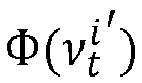
  • In this example, the first factor F1 i depends on the theoretical power Φ output from a wind turbine 15i exactly facing the wind W, which is preferably calculated according to the following equation: Φ ( v t i ) = 1 2 . ρ . A . ν t i 3 . C p ( v t i )
    Figure imgb0066
    where:
    • v t i
      Figure imgb0067
      is the local wind velocity of the ith wind turbine 15i at the initial time instant t,
    • ρ is the air density, in kg/m3,
    • A is the rotor blade area, and
    • Cp is a power coefficient respective of the wind turbine 15i.
  • The air density ρ, the rotor blade area A and the power coefficient Cp are preferably predefined.
  • In this example, the power coefficient Cp preferably defines a cut-in velocity value vcut-in and a cut-out velocity value vcut-out. In other words, if the local wind velocity v t i
    Figure imgb0068
    is smaller than the cut-in velocity value vcut-in, the wind turbine 15i does not output power since said velocity is not high enough to drive the blades. On the contrary, if the local wind velocity v t i
    Figure imgb0069
    is higher than the cut-out velocity value vcut-out, the power generated reaches a threshold and remains constant.
  • An example of a theoretical power curve is shown in Figure 4 representing the evolution of the theoretical power Φ as a function of the local wind velocity v t i
    Figure imgb0070
    for a wind turbine 15i perfectly facing the wind W.
  • In a preferred example, the first factor F1 i in addition takes into consideration that a yaw misalignment is possible between the wind W and the wind turbine 15i, i.e. α t + 1 i 0
    Figure imgb0071
    , the first factor F1 i then being preferably equal to the following equation F 1 i = Φ v t i . cos p α t + 1 i
    Figure imgb0072
    where:
    • p is a tunable parameter, and
    • cos p α t + 1 i
      Figure imgb0073
      is the cosine of the relative yaw angle α t + 1 i
      Figure imgb0074
      at the power of p.
  • Thus, in this example, the first contribution C1 i is preferably equal to
    Figure imgb0075
    where fpower is the function associating to a couple of local velocity v t i
    Figure imgb0076
    and relative yaw angle α t + 1 i
    Figure imgb0077
    , and estimation of the power output from the wind turbine 15i.
  • In the preceding example, the first component C1 is thus preferably equal to the sum of the first contribution C1 i of each wind turbine 15i, normalized by the number of wind turbines 15i, i.e. according to the following equation:
    Figure imgb0078
  • One can notice that considering the relative yaw angles α t + 1 i
    Figure imgb0079
    at the next time instant t + 1 instead of the relative yaw angles α t i
    Figure imgb0080
    at the initial time instant t, is just a convention choice to represent that the power considered is the power between said first time instant t and the next time instant t + 1.
  • In the considered example, it has not been defined yet how the local wind velocities ν t i
    Figure imgb0081
    may be obtained.
  • One way to determine the local wind velocities v t i
    Figure imgb0082
    is to proceed to a simulation of the wind flowing around the wind turbines 15i between time instants t and t + 1. This simulation, further denoted fsimulation, makes it possible to determine, for each wind turbine 15i, the local wind velocity v t i
    Figure imgb0083
    from the estimated general wind velocity V't, the wind direction K t
    Figure imgb0084
    and each relative yaw angle α t + 1 i i 0 ; N 1
    Figure imgb0085
    preferably such that: v t i = f simulation i K t V t α t + 1 i i 0 ; N 1
    Figure imgb0086
    where f simulation i
    Figure imgb0087
    is the simulation providing the local wind velocity ν t i
    Figure imgb0088
    of the ith wind turbine 15i.
  • For example, the simulation is performed via the open-source tool FLORIS (FLOw Redirection and Induction in Steady state), known per se.
  • Finally, merging equations [1], [2], [7] and [8], a complete form of the first component C1 is for example according to the following set of equations:
    Figure imgb0089
    with i 0 ; N 1
    Figure imgb0090
    v t i = f simulation i K t V t α t + 1 i i 0 ; N 1
    Figure imgb0091
    α t + 1 i = f yaw K t , β t + 1 i
    Figure imgb0092
    β t + 1 i = f control β t i u t i
    Figure imgb0093
  • Regarding the second component C2, one may consider propagating the equations of the first component C1 for further time instants t + k k 0 ; L
    Figure imgb0094
    , thus leading to an optimal second component C2* respecting the following set of equations:
    Figure imgb0095
    with k 1 ; L , i 0 ; N 1
    Figure imgb0096
    v t + k i = f simulation i K t + k V t + k α t + k + 1 i i 0 ; N 1
    Figure imgb0097
    α t + k + 1 i = f yaw K t + k , β t + k + 1 i
    Figure imgb0098
    β t + k + 1 i = f control β t + k i u t + k i
    Figure imgb0099
  • With such consideration, the optimization problem would be a MPC (Model Predictive Control) problem that may be written as follow:
    Figure imgb0100
    subject to u min u t + k i u max , k 0 ; L , i 0 ; N 1
    Figure imgb0101
    with k 0 ; L , i 0 ; N 1
    Figure imgb0102
    v t + k i = f simulation i K t + k , V t + k , α t + k + 1 i i 0 ; N 1
    Figure imgb0103
    α t + k + 1 i = f yaw K t + k , β t + k + 1 i
    Figure imgb0104
    β t + k + 1 i = f control β t + k i u t + k i
    Figure imgb0105
    where umin and umax are rotation command bounds that cannot be exceeded, forming a constraints of the problem.
  • The MPC problem is strongly complex since it takes into consideration, for each time instant t + k k 0 ; L
    Figure imgb0106
    , and for each wind turbine 15i, the corresponding local wind velocity v t + k i
    Figure imgb0107
    . As already presented, said local wind velocities v t + k i k 0 ; L , i 0 ; N 1
    Figure imgb0108
    depends on the wake effect, i.e. on the influence of other wind turbines 15i at preceding time instants.
  • In particular, for an arbitrary chosen wind turbines 15i and for an arbitrary chosen time instant t + k, the wake effect at said time instant t + k depends on the relative yaw angles α t + k + 1 i i 0 ; N 2
    Figure imgb0109
    of each wind turbines 15i, at the next time instant t + k + 1, i.e. on both the absolute yaw angles β t + k i i 0 ; N 1
    Figure imgb0110
    and the rotation commands u t + k i i 0 ; N 1
    Figure imgb0111
    at said time instant t + k, cf equations [1] and [2]. However, each absolute yaw angle β t + k i
    Figure imgb0112
    depends on the rotation commands u t + k 1 i
    Figure imgb0113
    at the preceding time instant, cf equation [1]. It leads that, determining the local wind velocities v t + k i i 0 ; N 1
    Figure imgb0114
    for time instants t + k, further than time instant t + 1, is strongly complex and requires a lot of simulations.
  • Consequently, the second component C2 is simplified compared to the optimal second component C2* so that the second component C2 depends on a calculated rotation command u ^ t + k i k 1 ; L
    Figure imgb0115
    for the wind turbines (15i) to rotate toward the estimated wind directions K t + k k 1 ; L
    Figure imgb0116
    for each further time instant t + k k 1 ; L
    Figure imgb0117
    .
  • Such calculated rotation command u ^ t + k i
    Figure imgb0118
    , is obtained by any controller able to determine analytically rotation commands from the other parameters. It is understood by "analytically", that it exists a formula for determining such command without any optimization.
  • For example, such calculated rotation command u ^ t + k i
    Figure imgb0119
    preferably respects the following equation, denoted naive controller: u ^ t + k i = clip f yaw K t + k β t + k + 1 i , u min , u max
    Figure imgb0120
    where clip is a clipping function.
  • In other words, clip is the function determining each calculated rotation command u ^ t + k i
    Figure imgb0121
    , as:
    • the one making the relative yaw angle α t + k + 1 i = f yaw K t + k , β t + k + 1 i
      Figure imgb0122
      equal to zero, if feasible, i.e. comprised between the lower umin and upper umax bounds, or
    • the one among the bounds umin, umax minimizing the relative yaw angle α t + k + 1 i =
      Figure imgb0123
      f yaw K t + k , β t + k + 1 i
      Figure imgb0124
      , else case.
  • Preferably, the second component C2 comprises, for each further time instant t + k k 1 ; L
    Figure imgb0125
    , a temporal variable C2 t+ k.
  • Preferably, the second component C2 is the sum of each temporal variable C2 t+k such that: C 2 = k = 1 L C 2 t + k
    Figure imgb0126
  • Each temporal variable C2 t+k comprises a second contribution C 2 t + k i
    Figure imgb0127
    for each wind turbine 15i.
  • Each second contribution C 2 t + k i i 0 ; N 1
    Figure imgb0128
    depends on an expected relative yaw angle α ^ t + k + 1 i
    Figure imgb0129
    between the wind turbine 15i and the wind direction K' t+ k, considering that the wind turbine 15i implemented the calculated rotation command u ^ t + k i
    Figure imgb0130
    .
  • To this end, compared to the optimal second component C2*, in each second contribution C 2 t + k i i 0 ; N 1
    Figure imgb0131
    , each relative yaw angle α t + k + 1 i
    Figure imgb0132
    , depending on the rotation command u t + k i
    Figure imgb0133
    , is replaced by the expected relative yaw angle α ^ t + k + 1 i
    Figure imgb0134
    if the naive controller was used instead. It reduces the complexity coming from the optimization, as the naive controller provide an explicit solution, i.e. a calculated rotation command u ^ t + k i
    Figure imgb0135
    without requiring solving an optimization problem but directly from a formula, as show in equation [12].
  • Preferably, the cosine function at power p of each relative yaw angle α t + k + 1 i
    Figure imgb0136
    is replaced with a simpler penalization for relative yaw misalignment. The penalization chosen corresponds to one minus the normalized, absolute value of that expected relative yaw angle α ^ t + k + 1 i
    Figure imgb0137
    . It provides linearity and a better interpretability. Mathematically, it corresponds, for each further time instant t + k to the following expression: 1 1 N . 1 180 . i = 0 N 1 α ^ t + k + 1 i
    Figure imgb0138
  • Optionally, the indicator function
    Figure imgb0139
    is removed so that there is no discontinuity. Even if an expected relative yaw angle α ^ t + k + 1 i
    Figure imgb0140
    is too great, it can be of some interest for the optimization to know about the potential power output. The more a wind turbine 15i is misaligned, the less likely it will be to produce energy and the more it will be penalized.
  • Preferably, each temporal variable C2 t+k comprises a factor γ k-1, denoted discount factor γ k-1, making decrease the influence, on the second component C2, of temporal variable C2 t+k as a function of the further time instants t + k k 1 ; L
    Figure imgb0141
    remoting from the initial time instant t. It gives more importance to temporal variables C2 t+k closed to the initial time instant t than to the temporal variables C2 t+k remote from the initial time instant t.
  • For example, the discount factor γ k-1 is formed by considering a predefined value γ at the power of: k minus 1. Preferably, the predefined value γ is comprised between 0 and 1.
  • Preferably, compared to the optimal second component C2*, in each of the temporal variable C2 t+ k, each local wind velocity v t + k i
    Figure imgb0142
    is replaced by any wind velocity which does not depend on any simulation process. As an example, each local wind velocity v t + k i
    Figure imgb0143
    is replaced by the estimated general wind velocity V' t+ k. This approximation corresponds to considering that for further time instants t + k, the wind W is received by each wind turbine 15i with the general wind velocity V t + k
    Figure imgb0144
    thus neglecting the wake effect for further time instants t + k. It reduces the complexity coming from the simulation since it is not require to use a simulation for time instants further than the initial time instant t.
  • In an example, each temporal variable C2 t+k is equal to: C 2 t + k = γ k 1 . Φ V t + k . 1 1 N . 1 180 . i = 0 N 1 α ^ t + k + 1 i
    Figure imgb0145
  • In said example, it leads that the second component C2 is equal to: C 2 = k = 1 L γ k 1 . Φ V t + k . 1 1 N . 1 180 . i = 0 N 1 α ^ t + k + 1 i
    Figure imgb0146
  • Finally, merging equations [1], [2], [12], and [16], a complete form of the second component C2 is for example according to the following set of equations: C 2 = k = 1 L γ k 1 . Φ V t + k . 1 1 N . 1 180 . i = 0 N 1 α ^ t + k + 1 i
    Figure imgb0147
    with: α ^ t + k + 1 i = f yaw K t + k β ^ t + k + 1 i
    Figure imgb0148
    β ^ t + k + 1 i = f control β ^ t + k i u ^ t + k i
    Figure imgb0149
    β ^ t + 1 i = f control β t i u t i
    Figure imgb0150
    u ^ t + k i = clip f yaw K t + k β t + k + 1 i , u min , u max
    Figure imgb0151
    In equations [17], the expression β ^ t + 1 i = f control β t i u t i
    Figure imgb0152
    ensures a continuity between the first C1 and the second C2 components.
  • The second component C2 forms an heuristic of the first component C1.
  • Because this heuristic C2 depends on neither the future optimized yaw settings (naive control), nor the future local velocities (no simulation), it does not increase complexity. The heuristic C2 is a scalar acting as a penalization for the optimization.
  • One may notice that the second component C2, i.e. the heuristic, only depends on:
    • the absolute yaw angle β t i
      Figure imgb0153
      of each wind turbine 15i at the initial time instant t,
    • on each rotation command u t i
      Figure imgb0154
      at said time instant first t,
    • the set V t + k k 1 ; L
      Figure imgb0155
      of estimated general wind velocities at each further time instant t + k k 1 ; L
      Figure imgb0156
      , and
    • the set K t + k k 1 ; L
      Figure imgb0157
      of estimated wind directions at each further time instant t + k k 1 ; L
      Figure imgb0158
      .
  • Actually, each calculated rotation command u ^ t + k i
    Figure imgb0159
    is open-loop determined, i.e. determined only based on the parameter of the heuristic C2 without requiring any optimization process.
  • In a sense, the heuristic C2 is the discounted, weighted sum of the future theoretical power outputs. Thus the heuristic C2 evaluates how well the wind turbines 15i will manage to stay aligned with the each estimated wind direction K' t+ k.
  • Based on the example of first C1 and second C2 components, the optimization problem solved by the calculating module 60, further denoted simplified optimization problem, is for example the following: max u t i i 0 , N 1 f obj = C 1 + C 2
    Figure imgb0160
    subject to u min u t i u max , i 0 ; N 1
    Figure imgb0161
    with k 0 , L , i 0 , L
    Figure imgb0162
    α ^ t + k + 1 i = f yaw K t + k β ^ t + k + 1 i
    Figure imgb0163
    β ^ t + k + 1 i = f control β ^ t + k i u ^ t + k i
    Figure imgb0164
    u ^ t + k i = clip f yaw K t + k β t + k + 1 i , u min , u max
    Figure imgb0165
    β ^ t + 1 i = f control β t i u t i
    Figure imgb0166
    v t i = f simulation i K t V t α t + 1 i i 0 ; N 1
    Figure imgb0167
    α t + 1 i = f yaw K t β t i
    Figure imgb0168
    β t + 1 i = f control β t i , u t i
    Figure imgb0169
  • Preferably, the calculating module 60 is configured to solve is the simplified optimization problem of equation [18].
  • One may notice that an advantage of the simplified optimization problem compared to the MPC problem, is that it considerably reduces the amount of parameter to optimize by only optimizing the rotation commands u t i
    Figure imgb0170
    at the initial time instant t. Actually, in the second component C2, the calculated rotation commands u ^ t + k i k 1 ; L , i 0 ; N 1
    Figure imgb0171
    are open-loop determined, i.e. it exists a formula determining each calculated rotation command u ^ t + k i
    Figure imgb0172
    from the other parameters of the simplified optimization problem, without requiring performing any optimization. In other words, given a rotation command u t i
    Figure imgb0173
    , it exists a unique set of calculated rotation commands u ^ t + k i k 1 ; L , i 0 ; N 1
    Figure imgb0174
    , each depending analytically on the other parameters, maximizing the second component C2.
  • The principle of said simplified optimization problem is represented in Figures 5 and 6.
  • In Figure 5, the x-axis represents the succession of time instants t + k k 0 ; 3
    Figure imgb0175
    . In particular, the abscissa axis represents four time instants t, t + 1, t + 2, t + 3. In this Figure, the y-axis corresponds to yaw angles β t i , β ^ t + 1 i , β ^ t + 2 i , β ^ t + 3 i
    Figure imgb0176
    and wind directions K't, K' t+1 , K' t+2 , K' t+3 of a chosen wind turbine 15i.
  • In Figure 4, the crosses corresponds to the absolute yaw angles β t i , β ^ t + 1 i , β ^ t + 2 i , β ^ t + 3 i
    Figure imgb0177
    at the successive time instants t + k k 0 ; 3
    Figure imgb0178
    . Each horizontal full line, starting from a respective cross, represents the projection the absolute yaw angle β t i , β ^ t + 1 i , β ^ t + 2 i
    Figure imgb0179
    , on the next time instant, if no control is performed, i.e. β ^ t + k + 1 i = β t + k i
    Figure imgb0180
    . At each further time instant, a distance between said projection and the corresponding cross, i.e. the actual value of the absolute yaw angle β ^ t + k + 1 i
    Figure imgb0181
    , is the rotation command u t + k i
    Figure imgb0182
    , or calculated rotation command u ^ t + k i
    Figure imgb0183
    at the preceding time instant.
  • The triangles 80 formed from each cross and extending until the next time instant correspond to the range of rotation command u t + k i
    Figure imgb0184
    that are feasible for the next time instant, such that the absolute yaw angle β ^ t + k + 1 i
    Figure imgb0185
    at the next time instant t + k + 1 is comprised between β ^ t + k i + u min
    Figure imgb0186
    and β ^ t + k i + u max
    Figure imgb0187
    . The limits of said triangle 80 are defined by the lower umin and upper umαx bounds.
  • Still in Figure 5, the circles corresponds to the estimated wind direction K t + k k 0 ; 3
    Figure imgb0188
    at each time instant t + k k 0 ; 3
    Figure imgb0189
    .
  • At each time instant t + k, the distance between the cross and the circle corresponds to the relative yaw angle α t + k i
    Figure imgb0190
    at said time instant t + k.
  • Figure 5 is divided into a first part 85 and a second part 90. The first part 85 corresponds to the first component C1 and the second part 90 corresponds to the second component C2 of the power quantity fobj.
  • The first part 85 only corresponds to the initial time instant t and the incidence, on the next time instant t + 1, of the rotation command u t i
    Figure imgb0191
    determined at said time instant t. The determination said rotation command u t i
    Figure imgb0192
    results from the optimization of the first component C1 as it is described below. Thus a real optimization is performed on the first part 85.
  • The second part 90 corresponds to the further time instants t + k k 1 ; 3
    Figure imgb0193
    and the expected absolute yaw angles β ^ t + k i k 1 ; 3
    Figure imgb0194
    induced by the calculated rotation commands u ^ t + k i k 1 ; 3
    Figure imgb0195
    determined by a naive controller. In other words, the calculated rotation commands u ^ t + k i k 1 ; 3
    Figure imgb0196
    are determined to reduce as much as possible, for each next time instant t + k + 1, the expected relative yaw angles α ^ t + k + 1 i
    Figure imgb0197
    .
  • Since each calculated rotation command u ^ t + k i k 1 ; 3
    Figure imgb0198
    is limited by the bounds umin, umax, it is clear that the rotation command u t i
    Figure imgb0199
    at the initial time instant t has an important incidence on the reachable expected relative yaw angles α ^ t + k i k 1 ; 3
    Figure imgb0200
    for further time instants t + k k 1 ; 3
    Figure imgb0201
    .
  • Figure 6 is the same figure as Figure 5 except that rotation command u t i
    Figure imgb0202
    at the initial time instant t is distinct as for Figure 5.
  • One may notice that such difference has a consequence each next time instants, resulting in higher expected relative yaw angles α ^ t + k i k 1 ; 3
    Figure imgb0203
    , and thus in a lower value of the second component C2.
  • By comparing Figure 5 and 6, one may better understand that the second component C2 forms a penalization of the first component C1 since the reached values of the second component C2 is strongly influenced by the optimization performed for the first component C1.
  • In the simplified optimization problem, by choosing certain rotation command u t i
    Figure imgb0204
    for the initial time instant t, the heuristic C2 uses a naive controller over a future time horizon of L time instants t + k to evaluate how well the wind turbines 15i will manage to stay aligned with the predicted wind directions K t+ k'.
  • For example, if the future expected power outputs are high, the heuristic C2 will encourage a rotation commands u t i
    Figure imgb0205
    that will put the wind turbines 15i in good orientations for the future. Thus, in such case the heuristic C2 will penalize the first component C1 for rotation commands u t i
    Figure imgb0206
    that would prevent wind turbines 15i from keeping track of the wind direction K t+ k'.
  • To solve the simplified optimization problem, the calculating module 60 is preferably configured to obtain, for each wind turbine 15i, one rotation command candidate u ˜ t i
    Figure imgb0207
    , denoted candidate u ˜ t i
    Figure imgb0208
    , forming a set of candidates u ˜ t i i 0 ; N 1
    Figure imgb0209
    comprising a respective candidate u ˜ t i
    Figure imgb0210
    for each wind turbines 15i .
  • The calculating module 60 is then configured to determine, the corresponding local velocity v t i
    Figure imgb0211
    , from:
    • the estimated wind direction K t
      Figure imgb0212
      ,
    • the estimated general velocity of the wind V t
      Figure imgb0213
      , and
    • each candidate u ˜ t i
      Figure imgb0214
      .
  • To this end, the calculating module 60 is for example configured to implement equations [1], [2] and [8]. In that case, the calculating module 60 is, by the way, configured to determine corresponding relative yaw angles α t + 1 i
    Figure imgb0215
    , preferably based on equation [2].
  • The calculating module 60 is configured to then calculate the first component C1, from each corresponding local velocity v t i
    Figure imgb0216
    , and preferably from the corresponding relative yaw angles α t + 1 i
    Figure imgb0217
    .
  • The calculating module 60 is in addition configured to determine, for each further time instant t + k, the corresponding calculated rotation command u ^ t + k i i 0 ; N 1
    Figure imgb0218
    from the estimated wind direction K t + k
    Figure imgb0219
    at said time instant t + k.
  • Preferably, the calculating module 60 is configured to implement equation [12]. In that case, the calculating module 60 is configured to determine each corresponding calculated rotation command u ^ t + k i
    Figure imgb0220
    in addition from the expected absolute yaw angle β ^ t + k i
    Figure imgb0221
    determined for the previous time instant t + k - 1. For each wind turbine 15i, the expected absolute yaw angle β ^ t + 1 i
    Figure imgb0222
    at the time instant t + 1 is preferably equal to the absolute yaw angle β t + 1 i
    Figure imgb0223
    at said time instant t + 1, i.e. determined based on equation [1].
  • The calculating module 60 is further configured to calculate the corresponding second component C2 from the corresponding calculated rotation commands u ^ t + k i
    Figure imgb0224
    , for example by implementing equation [16].
  • The calculating module 60 is configured to then calculate the corresponding power quantity fobj from the first C1 and second C2 components.
  • The calculating module 60 is thus configured to iterate the preceding determinations and calculations for a plurality of rotation command candidate sets u ˜ t i i 0 ; N 1
    Figure imgb0225
    .
  • The calculating module 60 is configured to then select the rotation commands u t i i 0 ; N 1
    Figure imgb0226
    as the set of rotation command candidate u ˜ t i i 0 ; N 1
    Figure imgb0227
    , maximizing the power quantity fobj.
  • The sending module 65 is configured to send each rotation command u t i
    Figure imgb0228
    determined by the calculating module 60, to the corresponding wind turbine 15i, and in particular to its yaw actuator, so that said yaw actuator implement the received rotation command.
  • The optional pretreatment module 67 is configured apply a treatment on the estimated wind directions K t + k k 0 ; L
    Figure imgb0229
    on the wind farm to obtain treated wind directions K t + k k 0 ; L
    Figure imgb0230
    . As an example the treatment is a low-pass filtering. This makes it possible to smooth the estimated wind directions K t + k k 0 ; L
    Figure imgb0231
    . With such treatment if a drastic change in the wind directions happens only for a short time, such change would not appear in the treated wind direction K t + k k 0 ; L
    Figure imgb0232
    as important as in the estimated wind directions K t + k k 0 ; L
    Figure imgb0233
    , since it would be damped by the low-pass filtering.
  • Preferably, the calculating module 60 is configured to perform its solving by using the treated wind directions K t + k k 0 ; L
    Figure imgb0234
    instead of the estimated wind directions K t + k k 0 ; L
    Figure imgb0235
    .
  • This is benefic since if the treated wind directions K t + k k 0 ; L
    Figure imgb0236
    were not considered, for further time instant t + k k 1 ; L
    Figure imgb0237
    , the simplified optimization problem aims a making the wind turbines tracking the estimated wind directions K t + k k 1 ; L
    Figure imgb0238
    . However, if the considered directions comprise a fast change, the corresponding calculated rotation command(s) u ^ t + k i
    Figure imgb0239
    would be clipped, i.e. equal to either umin or umax, while it is not long term profitable.
  • The functioning of wind farm 10 and in particular of the control system 20 will now be detailed by a control method 100 and in reference to figure 7 representing a flowchart of said control method 100.
  • At an initial time instant t, each wind turbines 15i has an absolute yaw angle β t i
    Figure imgb0240
    . Initially also, the general wind velocities V t + k k 0 ; L
    Figure imgb0241
    and wind directions K t + k k 0 ; L
    Figure imgb0242
    are estimated for each time instant t + k k 0 ; L
    Figure imgb0243
    over an horizon L, as previously described, preferably by the sensor 50.
  • The method 100 comprises a receiving step 110, during which the electronic control device 45 receives, for the set of successive time instants t + k k 0 ; L
    Figure imgb0244
    , the estimated general wind velocities V t + k k 0 ; L
    Figure imgb0245
    and the estimated wind directions K t + k k 0 ; L
    Figure imgb0246
    of the wind W, on the wind farm 10.
  • Optionally, during the receiving step 110, the electronic control device 45 in addition receives the absolute yaw angle β t i
    Figure imgb0247
    of each wind turbine 15i.
  • Optionally, the method comprises a pretreatment step 115, wherein the electronic control device 45 apply a treatment on the estimated wind directions K t + k k 0 ; L
    Figure imgb0248
    on the wind farm to obtain treated wind directions K t + k k 0 ; L
    Figure imgb0249
    . Preferably, the treatment is a low-pass filtering.
  • The method 100 then comprises a determining step 120, during which the electronic control device 45 determined, for each wind turbine 15i, the respective rotation command u t i
    Figure imgb0250
    from the set of estimated wind direction K t + k k 0 ; L
    Figure imgb0251
    and the set of velocity of the wind V t + k k 0 ; L
    Figure imgb0252
    on the wind farm 10, by solving an optimization problem as previously described.
  • The optimization problem aims at maximizing the power quantity fobj representative of a power generated by the wind farm 10 for said set of successive time instants t + k k 0 ; L
    Figure imgb0253
    , the power quantity fobj comprising a first component C1 and a second component C2.
  • The first component C1 depends on the local wind velocity ν t i
    Figure imgb0254
    at the contact of each wind turbine 15i at said initial time instant t, each local wind velocity ν t i
    Figure imgb0255
    depending on the rotation command u t i
    Figure imgb0256
    of each wind turbine 15i at said initial time instant t.
  • The second component C2 depends on a set of calculated rotation command u ^ t + k i k 1 ; L , i 1 ; N 1
    Figure imgb0257
    for the wind turbines 15i to rotate toward the estimated wind directions K t + k k 1 ; L
    Figure imgb0258
    for each further time instant t + k k 1 ; L
    Figure imgb0259
    .
  • If the control method 100 comprises the pretreatment step 115, during the determining step 120, the treated wind directions K t + k k 0 ; L
    Figure imgb0260
    are used instead of the estimated wind directions K t + k k 0 ; L
    Figure imgb0261
  • Preferably, said optimization problem is the simplified optimization problem of the set of equations [18].
  • To perform such solving, the determining step 120 preferably comprises an obtaining sub step 122, wherein, the electronic control device 45 obtains for each wind turbine 15i, a respective rotation command candidate u ˜ t i
    Figure imgb0262
    , forming the set of rotation command candidates u ˜ t i i 0 ; N 1
    Figure imgb0263
    for the wind farm 10, .
  • The set of rotation command candidates u ˜ t i i 0 ; N 1
    Figure imgb0264
    is preferably provided by gridding, for each wind turbine 15i, the space between the lower bound umin and the upper bound umax, by a predefined number of points.
  • The determining step 120 then comprises a first determining sub step 124, wherein the electronic control device 45 determines the first component C1 from each local wind velocity ν t i
    Figure imgb0265
    which depends on the set of obtained rotation command candidates u ˜ t i i 0 ; N 1
    Figure imgb0266
    .
  • Preferably, each local wind velocity ν t i
    Figure imgb0267
    is determined by performing a simulation of the wind W flowing in the wind farm, for example based on equation [8].
  • Preferably, the first component C1 is determined based on equation [7].
  • The determining step 120 then comprises a second determining sub step 126 wherein the electronic control device 45 determines the first component C2 from the calculated rotation commands u ^ t + k i i 0 ; N 1 , k 1 ; L
    Figure imgb0268
    . The calculated rotation command u ^ t + k i i 0 ; N 1 , k 1 ; L
    Figure imgb0269
    are the command aiming at making the wind turbines 15i tracking the estimated wind directions K t + k k 1 ; L
    Figure imgb0270
    for each further time instant t + k k 1 ; L
    Figure imgb0271
    .
  • Preferably, the calculated rotation command u ^ t + k i i 0 ; N 1 , k 1 ; L
    Figure imgb0272
    are determined from the estimated wind directions K t + k k 1 ; L
    Figure imgb0273
    and indirectly from the candidates u ˜ t i i 0 ; N 1
    Figure imgb0274
    , for example based on equations [12] and [1].
  • Preferably, the second component C2 is determined based on equation [16].
  • The determining step 120 further comprises a calculating sub step 128, wherein the electronic control device 45 calculates the power quantity fobj from the first C1 and second C2 components, preferably by summing said components C1, C2.
  • During the determining step 120, said obtaining 122, determining 124, 126 and calculating 126 sub steps are iterated from a plurality of rotation command candidate sets u ˜ t i i 0 ; N 1
    Figure imgb0275
    , thus leading to a respective power quantity fobj for each set u ˜ t i i 0 ; N 1
    Figure imgb0276
    . The new candidate set is preferably also obtained from the aforementioned gridding.
  • The determining step 120 then comprises a selecting sub step 129, wherein the rotation commands u t i i 0 ; N 1
    Figure imgb0277
    are selected as the set of rotation command candidate u ˜ t i i 0 ; N 1
    Figure imgb0278
    , maximizing the power quantity fobj.
  • The control method 100 then comprises a sending step 130, wherein the electronic control device 45 send the determined rotation command u t i
    Figure imgb0279
    to each respective wind turbine 15i for the rotation of each wind turbine 15i.
  • Optionally, the steps of the control method 100 are then iterated for the next time instant t + 1. As an example, in the next iteration, the initial time instant is the next time instant t + 1 of the preceding iteration. In the next iteration, the plurality of successive time instants extends from t + 1 until t + L + 1 so that the horizon, i.e. the number of time instants minus 1, remains equal to L.
  • Thanks to the electronic control device 45 and the control method 100 according to the invention, it possible to improve the wind farm control in order to output more power.

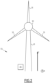
Claims (15)

  1. A control method (100) for controlling a wind farm (10) comprising a plurality of wind turbines (15i), based on a plurality of estimated general wind velocities V t + k k 0 ; L
    Figure imgb0280
    and a plurality of estimated wind directions K t + k k 0 ; L
    Figure imgb0281
    of the wind (W) on the wind farm (10),
    each wind turbine (15i) being configured, upon receiving a rotation command ( u t i
    Figure imgb0282
    ), to rotate, around an elongation axis (E) respective of the wind turbine (15i), according to said rotation command ( u t i
    Figure imgb0283
    ),
    the method (100) being implemented by an electronic control device (45) and comprising the following steps at an initial time instant (t):
    - receiving (110), for a set of successive time instants t + k k 0 ; L
    Figure imgb0284
    , estimated general wind velocities V t + k k 0 ; L
    Figure imgb0285
    and estimated wind directions K t + k k 0 ; L
    Figure imgb0286
    of wind (W), on the wind farm (10), each estimated general wind velocity and each estimated wind direction being associated to a respective time instant;
    - for said initial time instant (t), determining (120), for each wind turbine (15i), a respective rotation command u t i
    Figure imgb0287
    from the set of estimated wind directions K t + k k 0 ; L
    Figure imgb0288
    and the set of velocities of the wind V t + k k 0 ; L
    Figure imgb0289
    on the wind farm (10), by solving an optimization problem,
    the optimization problem aiming at maximizing a power quantity (fobj) representative of a power generated by the wind farm (10) for said set of successive time instants t + k k 0 ; L
    Figure imgb0290
    , the power quantity (fobj ) comprising a first component (C1) and a second component (C2),
    the first component (C1) depending on a local wind velocity ν t i
    Figure imgb0291
    at the contact of each wind turbine (15i) at said initial time instant (t), each local wind velocity ν t i
    Figure imgb0292
    depending on the rotation command u t i
    Figure imgb0293
    of each wind turbine (15i) at said initial time instant (t),
    the second component (C2) depending on a set of calculated rotation commands u ^ t + k i k 1 ; L , i 1 ; N 1
    Figure imgb0294
    for the wind turbines (15i) to rotate toward the estimated wind directions K t + k k 1 ; L
    Figure imgb0295
    for each further time instant t + k k 1 ; L
    Figure imgb0296
    ,
    - sending (130) the determined rotation command u t i
    Figure imgb0297
    to each respective wind turbine (15i) for the rotation of each wind turbine (15i).
  2. The control method (100) according to the preceding claim, wherein each local wind velocity ν t i
    Figure imgb0298
    is obtained by simulating the influence of each wind turbine (15i) on the wind (W) reaching the other wind turbines.
  3. The control method (100) according to claim 1 or 2, wherein each rotation command u t i
    Figure imgb0299
    is comprised between a lower bound (umin ) and an upper bound (umax ).
  4. The control method (100) according to any of the preceding claims, wherein the receiving (110), determining (120) and sending (130) steps are iterated several times.
  5. The method (100) according to any of the preceding claims, wherein the first component (C1) further depends on the relative yaw angle α t + 1 i
    Figure imgb0300
    between a blade's rotation axis (R) of each wind turbine (15i) and the wind direction (K't ),
    each relative yaw angle α t + 1 i
    Figure imgb0301
    being determined based on the rotation command u t i
    Figure imgb0302
    of the considered wind turbine (15i) at said initial time instant (t).
  6. The control method (100) according to claim 5, wherein the first component (C1) comprises a first contribution (C1 i ) for each wind turbine (15i),
    each first contribution (C1i) being equal to zero if the respective relative yaw angle α t + 1 i
    Figure imgb0303
    between a blade's rotation axis (R) of each wind turbine (15i) and the wind direction (Kt') is lower than a cut-in angle value (αcut-in ) or higher than a cut-out angle value (αcut-out ),
    each first contribution (C1 i ) depending on the local wind velocity v t i
    Figure imgb0304
    and the relative yaw angle α t + 1 i
    Figure imgb0305
    , if said relative yaw angle α t + 1 i
    Figure imgb0306
    is comprised between the cut-in angle value (αcut-in ) and the cut-out angle value (αcut-out ).
  7. The control method (100) according to claim 6, wherein the first component (C1) is equal to:
    Figure imgb0307
    wherein:
    Φ ν t i
    Figure imgb0308
    is the theoretical power (Φ) output from a wind turbine (15i) facing a wind with a local wind velocity v t i
    Figure imgb0309
    ,
    cos p α t + 1 i
    Figure imgb0310
    is the cosine of the relative yaw angle α t + 1 i
    Figure imgb0311
    at the power of p, representing the influence of a misalignement between the wind turbine (15i) and the wind direction (K't ),
    Figure imgb0312
    is the indicator function equal to 1 if the relative yaw angle α t i
    Figure imgb0313
    is comprised between the cut-in (αcut-in ) and cut-out (αcut-out ) angle values, and 0 else case, and
    N is the number of wind turbines (15i) in the wind farm (10).
  8. The control method (100) according to any of the preceding claims, wherein the second component (C2) comprises, for each further time instant t + k k 1 ; L
    Figure imgb0314
    , a temporal variable (C2 t+k ),
    each temporal variable (C2 t+k ) comprising a second contribution C 2 t + k i
    Figure imgb0315
    for each wind turbine (15i),
    each second contribution C 2 t + k i
    Figure imgb0316
    depending on an expected relative yaw angle α ^ t + k + 1 i
    Figure imgb0317
    between the wind turbine (15i) and the wind direction (K' t+k ), considering that the wind turbine (15i) implemented the calculated rotation command u ^ t + k i
    Figure imgb0318
    .
  9. The control method (100) according to claim 8, wherein each temporal variable (C2 t+k ) comprises a factor (γ k-1) making decrease the influence, on the second component (C2), of temporal variable (C2 t+k ) as a function of the further time instants t + k k 1 ; L
    Figure imgb0319
    remoting from the initial time instant (t).
  10. The control method (100) according to claim 8 or 9, wherein the second component (C2) is equal to C 2 = k = 1 L γ k 1 Φ V t + k 1 1 N 1 180 i = 0 N 1 α ^ t + k + 1 i
    Figure imgb0320
    wherein:
    y is a predefined value defining the factor (γ k-1),
    Φ(V' t+k ) is the theoretical power output from a wind turbine (15i) facing a wind with a general wind velocity equal to V t + k
    Figure imgb0321
    ,
    α ^ t + k + 1 i
    Figure imgb0322
    is the expected relative yaw angle at a further time instant t + k + 1,
    L is the number of considered time instants t + k k 0 ; L
    Figure imgb0323
    , and
    N is the number of wind turbines (15i) in the wind farm (10).
  11. The control method (100) according to any of the preceding claims, wherein, at each further time instant t + k k 1 ; L
    Figure imgb0324
    , each calculated rotation command u ^ t + k i
    Figure imgb0325
    is determined:
    - by aligning the wind turbine (15i) toward the wind direction K t + k
    Figure imgb0326
    if said calculated rotation command u ^ t + k i
    Figure imgb0327
    is comprised between a lower bound (umin ) and an upper bound (umax), or
    - by selecting, among the lower bound (umin ) and the upper bound (umax), the one minimizing the expected relative yaw angle α ^ t + k + 1 i
    Figure imgb0328
    else case.
  12. The control method (100) according to any of the preceding claims, wherein the step (120) of determining the rotation commands u t i i 0 ; N 1
    Figure imgb0329
    , comprises the following sub steps:
    - obtaining (122), for each wind turbine (15i), a respective rotation command candidate u ˜ t i
    Figure imgb0330
    , forming a set of rotation command candidates u ˜ t i i 0 ; N 1
    Figure imgb0331
    for the wind farm (10),
    - determining (124) the first component (C1) by:
    + determining, for each wind turbine (15i), the local wind velocity ν t i
    Figure imgb0332
    of said wind turbine (15i), from the estimated wind direction K t
    Figure imgb0333
    at the initial time instant (t), from the estimated general velocity of the wind V t
    Figure imgb0334
    at the initial time instant (t), and from the set of rotation command candidates u ˜ t i i 0 ; N 1
    Figure imgb0335
    ,
    + calculating the first component (C1) from each local wind velocity ν t i
    Figure imgb0336
    ,
    - determining (126) the second component (C2) by:
    + for each other further time instants t + k k 1 ; L
    Figure imgb0337
    , determining the calculated rotation command u ^ t + k i
    Figure imgb0338
    from the estimated wind direction K t + k
    Figure imgb0339
    at said time instant further (t + k),
    + calculating the second component (C2) from each calculated rotation commands u ^ t + k i
    Figure imgb0340
    , and
    - calculating (128) the power quantity (fobj ) from the first (C1) and second (C2) components,
    the sub steps of obtaining (122), determining (124, 126) and calculating (128) being iterated for a plurality of rotation command candidates sets u ˜ t i i 0 ; N 1
    Figure imgb0341
    ,
    the step (120) of determining the rotation command u t i i 0 ; N 1
    Figure imgb0342
    in addition comprising the sub step (129) of selecting the rotation commands u t i i 0 ; N 1
    Figure imgb0343
    as the set of rotation command candidate u ˜ t i i 0 ; N 1
    Figure imgb0344
    , maximizing the power quantity (fobj).
  13. The control method (100) according to any of the preceding claims, comprising between the receiving step (110) and the determining step (120), a pretreatment step (115), wherein a treatment is applied on the estimated wind directions K t + k k 0 ; L
    Figure imgb0345
    on the wind farm to obtain treated wind directions K t + k k 0 ; L
    Figure imgb0346
    ,
    the determining step (120) using the treated wind directions K t + k k 0 ; L
    Figure imgb0347
    instead of the estimated wind directions K t + k k 0 ; L
    Figure imgb0348
    ,
    preferably, the treatment being a low-pass filtering.
  14. A computer program product comprising instructions which, when being executed by a computer, implement a control method (100) according to any of the preceding claims.
  15. An electronic control device (45) for controlling a wind farm (10) comprising a plurality of wind turbines (15i), based on a plurality of estimated general wind velocities V t + k k 0 ; L
    Figure imgb0349
    and a plurality of estimated wind directions direction K t + k k 0 ; L
    Figure imgb0350
    of the wind (W) on the wind farm (10),
    each wind turbine (15i) being configured, upon receiving a rotation command u t i
    Figure imgb0351
    , to rotate, around an elongation axis (E) respective of the wind turbine (15i), accordingly with the rotation command u t i
    Figure imgb0352
    ,
    the electronic control device (45) comprising:
    - a receiving module (55) configured to receive, at an initial time instant (t), estimated general wind velocities V t + k k 0 ; L
    Figure imgb0353
    and estimated wind directions K t + k k 0 ; L
    Figure imgb0354
    of the wind, on the wind farm (10) for a set of successive time instants t + k k 0 ; L
    Figure imgb0355
    , each estimated general wind velocity V t + k k 0 ; L
    Figure imgb0356
    and each estimated wind direction K t + k k 0 ; L
    Figure imgb0357
    being associated to a respective time instant;
    - a calculating module (60) configured to determine, for said initial time instant (t), a respective rotation command u t i
    Figure imgb0358
    for each wind turbine (15i), from the set of estimated wind directions K t + k k 0 ; L
    Figure imgb0359
    and the set of estimated general wind velocities V t + k k 0 ; L
    Figure imgb0360
    on the wind farm (10), by solving an optimization problem,
    the optimization problem aiming at maximizing a power quantity (fobj ) representative of a power generated by the wind farm (10) for said set of successive time instants t + k k 0 ; L
    Figure imgb0361
    , the power quantity (fobj ) comprising a first component (C1) and a second component (C2),
    the first component (C1) depending on a local wind velocity ν t i
    Figure imgb0362
    at the contact of each wind turbine (15i) at said initial time instant (t), each local wind velocity ν t i
    Figure imgb0363
    depending on the rotation command u t i
    Figure imgb0364
    of each wind turbine (15i) at said initial time instant (t),
    the second component (C2) depending on a set of calculated rotation commands u ^ t + k i k 1 ; L , i 1 ; N 1
    Figure imgb0365
    for the wind turbines (15i) to rotate toward the estimated wind directions K t + k k 1 ; L
    Figure imgb0366
    for each further time instants t + k k 1 ; L
    Figure imgb0367
    ,
    - a sending module (65) configured to send the determined rotation command u t i
    Figure imgb0368
    to each respective wind turbine (15i) for the rotation of each wind turbine (15i).
EP23307225.5A 2023-12-15 2023-12-15 A control method for controlling a wind farm, related computer program product and electronic control device Pending EP4571099A1 (en)

Priority Applications (3)

Application Number Priority Date Filing Date Title
EP23307225.5A EP4571099A1 (en) 2023-12-15 2023-12-15 A control method for controlling a wind farm, related computer program product and electronic control device
PCT/EP2024/085976 WO2025125463A1 (en) 2023-12-15 2024-12-12 A control method for controlling a wind farm, related computer program product and electronic control device
TW113148602A TW202600965A (en) 2023-12-15 2024-12-13 A control method for controlling a wind farm, related computer program product and electronic control device

Applications Claiming Priority (1)

Application Number Priority Date Filing Date Title
EP23307225.5A EP4571099A1 (en) 2023-12-15 2023-12-15 A control method for controlling a wind farm, related computer program product and electronic control device

Publications (1)

Publication Number Publication Date
EP4571099A1 true EP4571099A1 (en) 2025-06-18

Family

ID=89542089

Family Applications (1)

Application Number Title Priority Date Filing Date
EP23307225.5A Pending EP4571099A1 (en) 2023-12-15 2023-12-15 A control method for controlling a wind farm, related computer program product and electronic control device

Country Status (3)

Country Link
EP (1) EP4571099A1 (en)
TW (1) TW202600965A (en)
WO (1) WO2025125463A1 (en)

Non-Patent Citations (5)

* Cited by examiner, † Cited by third party
Title
ANNONI JENNIFER ET AL: "Efficient Optimization of Large Wind Farms for Real-Time Control", 2018 ANNUAL AMERICAN CONTROL CONFERENCE (ACC), AACC, 27 June 2018 (2018-06-27), pages 6200 - 6205, XP033386982, DOI: 10.23919/ACC.2018.8430751 *
MEHDI VALI: "Adjoint-based model predictive control for optimal energy extraction in waked wind farms", CONTROL ENGINEERING PRACTICE., vol. 84, 1 March 2019 (2019-03-01), GB, pages 48 - 62, XP093161937, ISSN: 0967-0661, DOI: 10.1016/j.conengprac.2018.11.005 *
SIMLEY ERIC ET AL: "Wake Steering Wind Farm Control With Preview Wind Direction Information", 2021 AMERICAN CONTROL CONFERENCE (ACC), AMERICAN AUTOMATIC CONTROL COUNCIL, 25 May 2021 (2021-05-25), pages 1783 - 1789, XP033945911, DOI: 10.23919/ACC50511.2021.9483008 *
YIN XIUXING ET AL: "Data driven learning model predictive control of offshore wind farms", INTERNATIONAL JOURNAL OF ELECTRICAL POWER & ENERGY SYSTEMS, JORDAN HILL, OXFORD, GB, vol. 127, 11 December 2020 (2020-12-11), XP086455341, ISSN: 0142-0615, [retrieved on 20201211], DOI: 10.1016/J.IJEPES.2020.106639 *
YIN XIUXING ET AL: "Reliability aware multi-objective predictive control for wind farm based on machine learning and heuristic optimizations", ENERGY, ELSEVIER, AMSTERDAM, NL, vol. 202, 1 May 2020 (2020-05-01), XP086162807, ISSN: 0360-5442, [retrieved on 20200501], DOI: 10.1016/J.ENERGY.2020.117739 *

Also Published As

Publication number Publication date
WO2025125463A1 (en) 2025-06-19
TW202600965A (en) 2026-01-01

Similar Documents

Publication Publication Date Title
Sierra-García et al. Improving wind turbine pitch control by effective wind neuro-estimators
EP3613982B1 (en) Method for controlling operation of a wind turbine
US9702345B2 (en) Method of operating a wind turbine
US10683844B2 (en) Control of a wind turbine taking fatigue measure into account
US20220186709A1 (en) Reinforcement learning-based real time robust variable pitch control of wind turbine systems
EP3440346B1 (en) Control of a wind turbine taking noise into account
US9719494B2 (en) Methods of operating a wind turbine, wind turbines and wind parks
Saarinen et al. Field measurements and system identification of three frequency controlling hydropower plants
US20130302161A1 (en) Controller of wind turbine and wind turbine
US20240328387A1 (en) Methods and systems of closed loop collaborative wind plant control
US20140377065A1 (en) Method for controlling a wind turbine
CN114263565B (en) Yaw control equipment and method of wind generating set
EP2541052B1 (en) Controlling a wind turbine using a neural network function
US20230366377A1 (en) Method for controlling noise generated by a wind farm
CN114585950A (en) Method for computer-implemented forecasting of wind phenomena having an effect on a wind turbine
US12123400B2 (en) Modifying control strategy for control of a wind turbine using load probability and design load limit
CN107061164A (en) One kind considers the uncertain blower variable-pitch of executing agency away from Sliding Mode Adaptive Control method
EP4115079B1 (en) Control method and device of a wind park
US9903340B2 (en) System and method of controlling a wind turbine
CN118775150A (en) Method for controlling a wind farm using optimization methods
Amini et al. Control co-design of a hydrokinetic turbine: A comparative study of open-loop optimal control and feedback control
Pustina et al. Robustness of an economic nonlinear model predictive control for wind turbines under changing environmental and wear conditions
Simley Wind speed preview measurement and estimation for feedforward control of wind turbines
EP4166782A1 (en) Wind turbine model predictive control (mpc) with thrust and/or power correction
WO2025125463A1 (en) A control method for controlling a wind farm, related computer program product and electronic control device

Legal Events

Date Code Title Description
PUAI Public reference made under article 153(3) epc to a published international application that has entered the european phase

Free format text: ORIGINAL CODE: 0009012

STAA Information on the status of an ep patent application or granted ep patent

Free format text: STATUS: THE APPLICATION HAS BEEN PUBLISHED

AK Designated contracting states

Kind code of ref document: A1

Designated state(s): AL AT BE BG CH CY CZ DE DK EE ES FI FR GB GR HR HU IE IS IT LI LT LU LV MC ME MK MT NL NO PL PT RO RS SE SI SK SM TR

STAA Information on the status of an ep patent application or granted ep patent

Free format text: STATUS: THE APPLICATION IS DEEMED TO BE WITHDRAWN