EP4524778A1 - Computer program, apparatus, vehicle, and method for a bayes filter or smoother - Google Patents

Computer program, apparatus, vehicle, and method for a bayes filter or smoother Download PDF

Info

Publication number
EP4524778A1
EP4524778A1 EP23197459.3A EP23197459A EP4524778A1 EP 4524778 A1 EP4524778 A1 EP 4524778A1 EP 23197459 A EP23197459 A EP 23197459A EP 4524778 A1 EP4524778 A1 EP 4524778A1
Authority
EP
European Patent Office
Prior art keywords
parameter
distribution
observation
student
joint
Prior art date
Legal status (The legal status is an assumption and is not a legal conclusion. Google has not performed a legal analysis and makes no representation as to the accuracy of the status listed.)
Pending
Application number
EP23197459.3A
Other languages
German (de)
French (fr)
Inventor
Jonas Neuhöfer
Jörg Dr. Reichardt
Current Assignee (The listed assignees may be inaccurate. Google has not performed a legal analysis and makes no representation or warranty as to the accuracy of the list.)
Aumovio Germany GmbH
Original Assignee
Continental Automotive Technologies GmbH
Priority date (The priority date is an assumption and is not a legal conclusion. Google has not performed a legal analysis and makes no representation as to the accuracy of the date listed.)
Filing date
Publication date
Application filed by Continental Automotive Technologies GmbH filed Critical Continental Automotive Technologies GmbH
Priority to EP23197459.3A priority Critical patent/EP4524778A1/en
Priority to PCT/EP2024/075096 priority patent/WO2025056455A1/en
Publication of EP4524778A1 publication Critical patent/EP4524778A1/en
Pending legal-status Critical Current

Links

Images

Classifications

    • GPHYSICS
    • G06COMPUTING OR CALCULATING; COUNTING
    • G06FELECTRIC DIGITAL DATA PROCESSING
    • G06F17/00Digital computing or data processing equipment or methods, specially adapted for specific functions
    • G06F17/10Complex mathematical operations
    • G06F17/18Complex mathematical operations for evaluating statistical data, e.g. average values, frequency distributions, probability functions, regression analysis
    • GPHYSICS
    • G06COMPUTING OR CALCULATING; COUNTING
    • G06FELECTRIC DIGITAL DATA PROCESSING
    • G06F18/00Pattern recognition
    • G06F18/20Analysing
    • G06F18/24Classification techniques
    • G06F18/241Classification techniques relating to the classification model, e.g. parametric or non-parametric approaches
    • G06F18/2415Classification techniques relating to the classification model, e.g. parametric or non-parametric approaches based on parametric or probabilistic models, e.g. based on likelihood ratio or false acceptance rate versus a false rejection rate
    • G06F18/24155Bayesian classification
    • GPHYSICS
    • G06COMPUTING OR CALCULATING; COUNTING
    • G06VIMAGE OR VIDEO RECOGNITION OR UNDERSTANDING
    • G06V20/00Scenes; Scene-specific elements
    • G06V20/50Context or environment of the image
    • G06V20/56Context or environment of the image exterior to a vehicle by using sensors mounted on the vehicle

Definitions

  • Embodiments of the present disclosure relate to a computer program, an apparatus, a vehicle, and a method for a Bayes filter or smoother.
  • the proposed concept relates to an approach for determining an object state using a joint Student's t-distribution for an object state estimate in a previous time step, a process noise, and an observation of the object state.
  • Bayes filter and smoother play an increasingly important role in processing data, e.g., sensor data.
  • data e.g., sensor data.
  • Bayes filter and smoother play an increasingly important role in processing data, e.g., sensor data.
  • they are applied in robotics, assisted or autonomous driving systems, and signal processing.
  • true state dynamic quantities that are of interest
  • This unreliability can be caused by sensor limitations (e.g., estimating 3D coordinates or velocities from a 2D static image), sensor uncertainty/noise (e.g. when deciding which radar/lidar measurements were produced by the same object) and the dynamic nature of the processes involved (i.e. the underlying state will have changed between two observations).
  • sensor limitations e.g., estimating 3D coordinates or velocities from a 2D static image
  • sensor uncertainty/noise e.g. when deciding which radar/lidar measurements were produced by the same object
  • the dynamic nature of the processes involved i.e. the underlying state will have changed between two observations.
  • Some quantities also can't be measured directly (e.g., accelerations) and have to be inferred over multiple time steps.
  • Bayesian filtering which provides for using past observations to create a probability distribution of the most likely true state at a current timestep. This may require two models: one that shows how the system's state changes over time and another that shows how observations are produced from the true state. Additional stochastic 'process noise' and 'observation noise' models are used to account for model errors and non-deterministic processes.
  • the most common realization of this approach is the Kalman Filter, which assumes all stochastic models (i.e., state estimates, process noise and observation noise) to be Gaussian distributions. This has the advantage that all transformations of these probability distributions can be performed analytically, which results in a very efficient algorithm.
  • the distribution of observation noise is not Gaussian, and measurements are contaminated with outliers, i.e., measurements that are highly improbable under the Gaussian noise assumption.
  • outliers i.e., measurements that are highly improbable under the Gaussian noise assumption.
  • high-level functions such as object detection from camera data
  • very inaccurate or simply wrong measurements come about, which a system based on Gaussian distributions is unable to handle.
  • Outlier measurements in the naive Kalman Filter will result in extremely unrealistic state estimations since the algorithm explains the observed outlier as a combination of both an extremely large process noise and extremely large observation noise.
  • a standard heuristic is to simply ignore measurements outside a confidence region around the current state, a method which is called 'gating'.
  • some concepts use Gaussian distributed observation noise, where the covariance matrix itself is a random variable. They proposed Variational Bayes approaches to alternatively estimate the unknown covariance matrix and the updated state vector. Some other concepts apply a gating scheme for further stabilization.
  • the noise distribution used may have a closed form description even without further knowledge of the sampled covariance matrix.
  • This distribution is called Student-t distribution.
  • This distribution can be used to develop an outlier robust filter using Bayes rule and the inherited properties from the Gaussian distribution. However, these properties can only be exploited when also having Student-t state estimate and process noise models.
  • the Student-t distribution may be approximated by a mixture model of a Gaussian distribution and an outlier producing distribution with large covariance (either Student-t or Gaussian). Estimating how likely each distribution produced the observation allows for an informed convex combination of state updates from both models. This can be interpreted as a 'soft-gating' scheme.
  • Variational Bayes or general convex optimization methods can easily become computationally intensive, especially if they require many matrix multiplications and inversions or require the convergence of high-dimensional parameters.
  • the covariance matrix can only make weak statements about the relation between the true state and observed sample, estimations of the covariance matrix may be too uncertain.
  • Some concepts provide for filters based on the Student-t distribution that show similar behavior as the naive Kalman Filter in that the estimated means still follow all outliers, resulting in impossible 'jumping' trajectories.
  • embodiments of the proposed method provide for obtaining an analytic description of a Student-t distribution approximating the joint distribution of an object state estimate of a previous time step, an unknown process noise affecting the change of the object state in between the timesteps and an unknown observation noise affecting the quality of the observation of the object state.
  • the method comprises defining two parameters for the approximating joint distribution (in this context synonymously used for joint Student's t-distribution), defining their value given perfect knowledge of the unknown noises and true object state, and finding good approximations of these values based on the available observations.
  • the joint Student's t-distribution provides that the filter or smoother is less sensitive to outliers.
  • the first and the second parameter allow a less computationally intensive solution for the object state. So, the present approach provides a resource efficient and outlier robust solution for Bayes filter and smoother. This may result in a more accurate estimate of the object state and, therefore, in an improved performance of an application of the filter or smoother.
  • the Bayes filter or smoother may be applied in automotive applications, e.g., in an assisted or autonomous driving system, for sensing a vehicle's environment.
  • the proposed approach e.g., provides a more accurate estimate of the vehicle's environment and, so, allows for a more appropriate interaction of the vehicle with its environment.
  • the proposed approach may profit from the benefits of the proposed approach, too.
  • the first parameter is a parameter for the object state estimate and the process noise and the second parameter is a parameter for the process noise.
  • the first parameter is a parameter for the object state estimate and the process noise
  • the second parameter is a parameter for the process noise.
  • other ways of parametrization may be applied.
  • the joint Student's t-distribution is: t ⁇ x t ⁇ 1 v t e t
  • Determining the state of the object based on a joint Student's t-distribution may comprise solving the joint Student's t-distribution based on an approximation for the first and the second parameter.
  • the approximation e.g., comprises adjusting the first and the second parameter based on the observation and one or more previous approximations.
  • the observation may be indicative of sensor data of a first and at least one second sensor
  • the proposed method may be applied for fusing the sensor data of the first and the second sensor.
  • the proposed approach may provide more accurate fused sensor data than other approaches based on Gaussian distributions.
  • the method is for the use of a vehicle, and wherein the observation is indicative of sensor data from one or more sensors of the vehicle.
  • the proposed approach e.g., is applied in automotive implementations. Accordingly, it may be used to characterize a traffic environment, e.g., on (public) roads. Accordingly, the object state may be an object state of an object in such an environment, e.g., of a traffic participant.
  • the proposed method may be also applied in other applications and for other objects.
  • the proposed approach may be applied for characterizing a traffic area, e.g., for classifying and/or tracking objects in the traffic area. Accordingly, the observation may be indicative of one or more traffic participants, e.g., of their motion. Hence, the state may indicate a position and/or motion of the traffic participant.
  • the proposed approach e.g., allows to determine the position and/or motion more accurately.
  • the proposed approach e.g., is applied in assisted or autonomous driving system (ADS) for this purpose. In doing so, the proposed approach provides a higher performance of the ADS, e.g., such that the ADS may classify and/or track surrounding objects (e.g., traffic participants) more accurately and/or reliably.
  • ADS assisted or autonomous driving system
  • the proposed method may be executed by a computer. So, the proposed method may be a computer-implemented method.
  • embodiments of the present disclosure may provide a computer program comprising instructions which, when the computer program is executed by a computer, cause the computer to carry out the method of any one of the preceding claims.
  • inventions provide an apparatus comprising one or more interfaces for communication and a data processing circuit configured to execute the proposed method.
  • the proposed method may be installed on a vehicle.
  • embodiments may provide a vehicle comprising the proposed apparatus.
  • a Bayes filter is a probabilistic algorithm used for state estimation in systems where uncertainty is present. It utilizes Bayes' theorem to update an estimate about a state of the system based on a new observation.
  • the Bayes filter usually provides for two steps: prediction and update.
  • the filter uses a dynamic model of the system to project the current state forward in time while taking into account an uncertainty of such prediction.
  • the update step it combines the predicted state with the observation using Bayes' theorem to calculate a posterior estimate distribution while taking into account an uncertainty of the observation.
  • the proposed approach provides for a method of a Bayes filter or smoother, as laid out in more detail below with reference to Fig. 1 .
  • Fig. 1 shows a flow chart schematically illustrating a method 100 for a Bayes filter or smoother.
  • the method 100 comprises obtaining 110 an observation of an object state.
  • the observation e.g., is indicative of sensor data. So, for the observation, e.g., sensor data of one or more sensors is obtained.
  • the observation may include the sensor data in a raw or processed form.
  • the proposed approach e.g., is applied in an ADS for tracking traffic participants in an environment of a vehicle.
  • the sensor data e.g., is sensor data from environmental sensors for determining a position and/or motion of traffic participants.
  • the object state may indicate a position and/or motion and the observation may be indicative of a measurement (sensor data) of the position and/or motion.
  • the method 100 further provides for determining 120 the object state based on a joint Student's t-distribution.
  • determining the object state comprises approximating the joint Student's t-distribution of distributions for an object state estimate in a previous time step, a process noise, and the observation.
  • the joint Student's t-distribution is based on a first and at least one second parameter and determining the object state comprises adapting the first parameter and the second parameter.
  • the joint Student's t-distribution exhibits fatter tails than other distributions such as a Gaussian distribution. So, the joint Student's t-distribution make the filter or smoother more robust to outliers in the observation.
  • Bayes filter often is a Kalman filter. Therefore, examples of the proposed approach are described in more detail in connection with applications in the Kalman filter. However, the skilled person will appreciate that the present approach may be also applied in other Bayes filters or smoothers.
  • a multivariate student-t distribution t v ( ⁇ , ⁇ ) has the density t ⁇ x
  • ⁇ , ⁇ ⁇ ⁇ + p 2 ⁇ ⁇ 2 ⁇ p 2 ⁇ p 2 det ⁇ 1 + 1 ⁇ x ⁇ ⁇ T ⁇ ⁇ 1 x ⁇ ⁇ ⁇ + p 2 , where v is the degree of freedom discussed further down and p is the dimension of ⁇ , i.e., ⁇ is a p ⁇ p matrix.
  • is the scale matrix, which can be seen as a scaled form of the covariance matrix.
  • the Student's t-distribution may be seen as a generalization of the multivariate normal distribution N ⁇ ⁇ in the sense that a random variable X ⁇ t v ( ⁇ , ⁇ ) can be seen as being Gaussian X ⁇ N ⁇ ⁇ with unknown precision/covariance matrix ⁇ . That is, ⁇ is in itself a random variable with Wishart distribution W ( ⁇ / v,v ) .
  • the Wishart distribution is a positive-definite-matrix-valued distribution, which generalizes the one-dimensional concept of the gamma distribution and the ⁇ - squared distribution with v degrees of freedom.
  • the Student's t-distribution inherits a few properties from the multivariate normal distribution:
  • the parameterization of these distributions is the same as the parameterization in the multivariate normal case, with the two exceptions.
  • the degrees of freedom increase with conditioning i.e. conditioned Student's t-distribution are closer to normal distributions.
  • the covariance matrix of the conditioned matrix is weighted by the squared Mahalanobis distance X ⁇ ⁇ x T ⁇ xx ⁇ 1 X ⁇ ⁇ x of the observation X to the expectation ⁇ x in such a way that the covariance matrix can at most shrink by a factor of ⁇ ⁇ + p z but can increase to capture the degree of uncertainty an outlier brings.
  • a t and b t are estimated/approximated to solve the joint Student's t-distribution.
  • y t , a t , b t overestimates the most likely Mahalanobis distance due to the heavy tail and asymmetry of the distribution of e t T R t ⁇ 1 e t
  • y t , a t , b t + m T R t ⁇ 1 m 2 with the initial guess a t 0 ⁇ + p y ⁇ + y t ⁇ HF ⁇ t ⁇ 1 T R t ⁇ 1 y t ⁇ HF ⁇ t ⁇ 1 .
  • e ⁇ R t ⁇ 1 2 e ⁇ has distribution t ⁇ + p y e ⁇
  • HFF t -1 F T H T and HQ t H T can be pre-computed and each iteration of finding a t and b t may only require a single p y ⁇ p y matrix inversion, no additional matrix multiplication and otherwise on matrix-vector and component-wise matrix-multiplications (which are of the order of p y 2 and basically free).
  • a second step 220 the joint Student's t-distribution for the current time step is determined to find an approximation of it for values of the parameters a ( e t ) and b ( e t , x t ).
  • step 230 an initial guess for the parameters is made, as laid out above in more detail. Further, in a next step 240, the parameters are refined.
  • the change of the refinement is checked in another step 250. In order to do so, the change, e.g., is compared to a predefined threshold. In the case, the refinement changes the parameters significantly, they are refined further. If they do not change significantly, the parameters are used to solve the joint Student's t-distribution to determine the object state.
  • step 270 provides for checking if t ⁇ T and to stop if t is greater than T.
  • the process may be executed continuously. In such embodiments, step 270 may be omitted.
  • the proposed approach e.g., may be implemented in a computer program to execute steps of the method using a computer.
  • x t F t x t ⁇ 1 + v t v t ⁇ t ⁇ + n + m 0
  • Q t y t H t x t + e t e t ⁇ t ⁇ 0 R t
  • features and aspects of the described examples can be transferred to data smoothers, e.g., fixed-interval smoothers for data.
  • Bayes filter e.g., are used in sensor data fusion where sensor data of two or more sensor is fused. Accordingly, the proposed approach may be applied for fusing sensor data of a first and at least one second sensor. However, applications of the proposed approach are not only limited to sensor data fusion but may also include other use cases.
  • the proposed smoother uses a joint Student's t-distribution of two subsequent object state estimations x t and x t +1 of a current time step t and a subsequent time step t + 1.
  • the joint Student's t-distribution can be derived by: t ⁇ + p y x t
  • 0 Q t + 1 t ⁇ + p y x t v t + 1
  • b t + 1 is again ⁇ + p y + p x ⁇ + p y + x t ⁇ ⁇ t T P t ⁇ 1

Landscapes

  • Engineering & Computer Science (AREA)
  • Physics & Mathematics (AREA)
  • Data Mining & Analysis (AREA)
  • General Physics & Mathematics (AREA)
  • Theoretical Computer Science (AREA)
  • Evolutionary Biology (AREA)
  • Mathematical Physics (AREA)
  • Life Sciences & Earth Sciences (AREA)
  • Probability & Statistics with Applications (AREA)
  • Bioinformatics & Cheminformatics (AREA)
  • Bioinformatics & Computational Biology (AREA)
  • Pure & Applied Mathematics (AREA)
  • Mathematical Optimization (AREA)
  • Mathematical Analysis (AREA)
  • General Engineering & Computer Science (AREA)
  • Computational Mathematics (AREA)
  • Evolutionary Computation (AREA)
  • Multimedia (AREA)
  • Operations Research (AREA)
  • Computer Vision & Pattern Recognition (AREA)
  • Algebra (AREA)
  • Artificial Intelligence (AREA)
  • Databases & Information Systems (AREA)
  • Software Systems (AREA)
  • Radar Systems Or Details Thereof (AREA)
  • Complex Calculations (AREA)

Abstract

Embodiments of the present disclosure relate to a computer program, an apparatus, a vehicle, and a method for a Bayes filter or smoother. The method comprises obtaining an observation of an object state. Further, the method comprises determining the object state based on a joint Student's t-distribution. Determining the object state comprises approximating the joint Student's t-distribution of distributions for an object state estimate in a previous time step, a process noise, and the observation. The joint Student's t-distribution is based on a first and at least one second parameter. Determining the object state comprises adapting the first parameter and the second parameter.

Description

  • Embodiments of the present disclosure relate to a computer program, an apparatus, a vehicle, and a method for a Bayes filter or smoother. In particular, the proposed concept relates to an approach for determining an object state using a joint Student's t-distribution for an object state estimate in a previous time step, a process noise, and an observation of the object state.
  • Bayes filter and smoother play an increasingly important role in processing data, e.g., sensor data. In practice, e.g., they are applied in robotics, assisted or autonomous driving systems, and signal processing.
  • Particularly in those fields such as robotics, autonomous systems, and signal processing, one problem is the unreliability of measurements of dynamic quantities that are of interest (collectively called "true state"), such as the position of a foreign object, its velocity and its acceleration. This unreliability can be caused by sensor limitations (e.g., estimating 3D coordinates or velocities from a 2D static image), sensor uncertainty/noise (e.g. when deciding which radar/lidar measurements were produced by the same object) and the dynamic nature of the processes involved (i.e. the underlying state will have changed between two observations). Some quantities also can't be measured directly (e.g., accelerations) and have to be inferred over multiple time steps.
  • One attempt to solve this problem is Bayesian filtering which provides for using past observations to create a probability distribution of the most likely true state at a current timestep. This may require two models: one that shows how the system's state changes over time and another that shows how observations are produced from the true state. Additional stochastic 'process noise' and 'observation noise' models are used to account for model errors and non-deterministic processes. The most common realization of this approach is the Kalman Filter, which assumes all stochastic models (i.e., state estimates, process noise and observation noise) to be Gaussian distributions. This has the advantage that all transformations of these probability distributions can be performed analytically, which results in a very efficient algorithm.
  • However, in many real-world scenarios, the distribution of observation noise is not Gaussian, and measurements are contaminated with outliers, i.e., measurements that are highly improbable under the Gaussian noise assumption. Especially in high-level functions, such as object detection from camera data, very inaccurate or simply wrong measurements come about, which a system based on Gaussian distributions is unable to handle. Outlier measurements in the naive Kalman Filter will result in extremely unrealistic state estimations since the algorithm explains the observed outlier as a combination of both an extremely large process noise and extremely large observation noise.
  • A standard heuristic is to simply ignore measurements outside a confidence region around the current state, a method which is called 'gating'.
  • Other methods are based on intuitive concepts. For example, they focus on the aspect that outliers cannot be reasonably explained by Gaussian models. Some of them therefore propose to simply increase the observation noise covariance matrix at the timestep of the outlier until it can be explained reasonably. Some extend this approach by also considering outliers in the underlying process. Further ones introduce 'stochastic similarity measures' to maximize the similarity between predicted future state and updated state after consideration of the observation, as well as the similarity of expected observation and actual observation.
  • However, this intuitive character makes it difficult to understand why and how reliable these methods work and more importantly, how to improve them and how to adapt their advantages to other methods and use cases.
  • Alternatively, one can derive filtering algorithms replacing the Gaussian assumption with more realistic observation noise models, which can produce outliers. In particular, some concepts use Gaussian distributed observation noise, where the covariance matrix itself is a random variable. They proposed Variational Bayes approaches to alternatively estimate the unknown covariance matrix and the updated state vector. Some other concepts apply a gating scheme for further stabilization.
  • Furthermore, the noise distribution used may have a closed form description even without further knowledge of the sampled covariance matrix. This distribution is called Student-t distribution. This distribution can be used to develop an outlier robust filter using Bayes rule and the inherited properties from the Gaussian distribution. However, these properties can only be exploited when also having Student-t state estimate and process noise models. The Student-t distribution may be approximated by a mixture model of a Gaussian distribution and an outlier producing distribution with large covariance (either Student-t or Gaussian). Estimating how likely each distribution produced the observation allows for an informed convex combination of state updates from both models. This can be interpreted as a 'soft-gating' scheme.
  • For cases, where the covariance matrix changes unpredictably but slowly over time, an 'interacting multiple model' approach may be used. However, this does not apply to some use cases, e.g., in automotive applications for environment sensing where the covariance matrix may change rapidly.
  • Some of the concepts depend on various hyperparameters without clear guidance or intuition on their effects, such that they must be tweaked manually for each application on a subset of the actual problem set. And that without guarantees on the generality of their performance. Especially, similarity measures must be chosen arbitrarily, without any clear understanding of how the choice of different functions will affect the outcome.
  • Iterations in the Variational Bayes or general convex optimization methods can easily become computationally intensive, especially if they require many matrix multiplications and inversions or require the convergence of high-dimensional parameters.
  • Furthermore, since the covariance matrix can only make weak statements about the relation between the true state and observed sample, estimations of the covariance matrix may be too uncertain.
  • "Gating" and "soft-gating" methods have the real risk of following noisy measurements on a tangent away from the true state and then classifying all further actual reliable measurements as outliers and ignore them.
  • Some concepts provide for filters based on the Student-t distribution that show similar behavior as the naive Kalman Filter in that the estimated means still follow all outliers, resulting in impossible 'jumping' trajectories.
  • Further approaches require the calculation of integrals that can only be solved numerically which is highly computationally intensive.
  • Hence, there may be a demand for an improved concept of a Bayes filter or smoother to overcome the above problems.
  • This demand may be satisfied by the subject-matter of the appended independent patent claims. Further beneficial embodiments are disclosed in the dependent patent claims.
  • Embodiments of the present disclosure provide a method for a Bayes filter or smoother. The method comprises obtaining an observation of an object state. Further, the method comprises determining the object state based on a joint Student's t-distribution. Determining the object state comprises approximating the joint Student's t-distribution of distributions for an object state estimate in a previous time step, a process noise, and the observation. The joint Student's t-distribution is based on a first and at least one second parameter. Determining the object state comprises adapting the first parameter and the second parameter.
  • For this, embodiments of the proposed method provide for obtaining an analytic description of a Student-t distribution approximating the joint distribution of an object state estimate of a previous time step, an unknown process noise affecting the change of the object state in between the timesteps and an unknown observation noise affecting the quality of the observation of the object state. In more detail, the method comprises defining two parameters for the approximating joint distribution (in this context synonymously used for joint Student's t-distribution), defining their value given perfect knowledge of the unknown noises and true object state, and finding good approximations of these values based on the available observations.
  • On one hand, the joint Student's t-distribution provides that the filter or smoother is less sensitive to outliers. On the other hand, the first and the second parameter allow a less computationally intensive solution for the object state. So, the present approach provides a resource efficient and outlier robust solution for Bayes filter and smoother. This may result in a more accurate estimate of the object state and, therefore, in an improved performance of an application of the filter or smoother. In practice, the Bayes filter or smoother may be applied in automotive applications, e.g., in an assisted or autonomous driving system, for sensing a vehicle's environment. In such applications, the proposed approach, e.g., provides a more accurate estimate of the vehicle's environment and, so, allows for a more appropriate interaction of the vehicle with its environment. However, a skilled person will appreciate that other applications may profit from the benefits of the proposed approach, too.
  • In practice, the first parameter is a parameter for the object state estimate and the process noise and the second parameter is a parameter for the process noise. However, also other ways of parametrization may be applied.
  • In some embodiments, the joint Student's t-distribution is: t ν x t 1 v t e t | μ t 1 0 0 , a t P t 1 0 0 0 a t b t Q t 0 0 0 R t
    Figure imgb0001
    , wherein Qt represents a process covariance for the process noise, P t-1 represents a covariance of the object state estimate, at represents the first parameter, bt represents the second parameter, x t-1 represents the object state estimate, vt represents the process noise, et represents an observation uncertainty, µ t-1 represents the mean state for the object state estimate at the previous time step, and Rt represents a covariance for the observation uncertainty.
  • Determining the state of the object based on a joint Student's t-distribution may comprise solving the joint Student's t-distribution based on an approximation for the first and the second parameter.
  • The approximation, e.g., comprises adjusting the first and the second parameter based on the observation and one or more previous approximations.
  • In practice, the first parameter, e.g., is a t = ν + p y ν + e t T R t 1 e t
    Figure imgb0002
    and the second parameter is b t = ν + p y + p x ν + p y + x t 1 μ t 1 T P t 1 1 ( x t 1 μ t 1 .
    Figure imgb0003
  • The approximation, e.g., comprises obtaining an initial guess for the first and the second parameter, wherein the initial guess for the first parameter is a t 0 =
    Figure imgb0004
    ν + p y ν + y t HFμ t 1 T R t 1 y t HFμ t 1
    Figure imgb0005
    , and the initial guess for the second parameter is b t 0 =
    Figure imgb0006
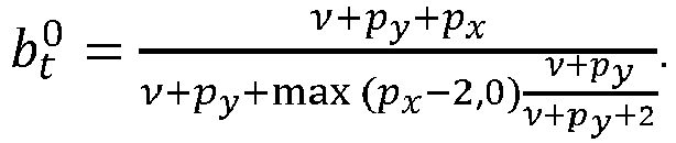
    ν + p y + p x ν + p y + max p x 2,0 ν + p y ν + p y + 2
    Figure imgb0007
    , wherein yt represents a state observation indicative of the observation, v, py, and px represent degrees of freedom (px and py denote the dimension of the object state xt and of the observation y, respectively), Rt represents a covariance for the observation uncertainty, µ t-1 represents the mean state for the state estimate at the previous time step, H represents an observation model, and F represents a transition model. Further, the approximation comprises refining the initial guess for the first and the second parameter.
  • In practice, the observation may be indicative of sensor data of a first and at least one second sensor, and the proposed method may be applied for fusing the sensor data of the first and the second sensor. In doing so, the proposed approach may provide more accurate fused sensor data than other approaches based on Gaussian distributions.
  • In some embodiments, the method is for the use of a vehicle, and wherein the observation is indicative of sensor data from one or more sensors of the vehicle.
  • As mentioned above, the proposed approach, e.g., is applied in automotive implementations. Accordingly, it may be used to characterize a traffic environment, e.g., on (public) roads. Accordingly, the object state may be an object state of an object in such an environment, e.g., of a traffic participant. However, the skilled person will appreciate that the proposed method may be also applied in other applications and for other objects.
  • In particular, the proposed approach may be applied for characterizing a traffic area, e.g., for classifying and/or tracking objects in the traffic area. Accordingly, the observation may be indicative of one or more traffic participants, e.g., of their motion. Hence, the state may indicate a position and/or motion of the traffic participant. In such applications, the proposed approach, e.g., allows to determine the position and/or motion more accurately. The proposed approach, e.g., is applied in assisted or autonomous driving system (ADS) for this purpose. In doing so, the proposed approach provides a higher performance of the ADS, e.g., such that the ADS may classify and/or track surrounding objects (e.g., traffic participants) more accurately and/or reliably.
  • In practice, one, more, or all steps of the proposed method may be executed by a computer. So, the proposed method may be a computer-implemented method.
  • Accordingly, embodiments of the present disclosure may provide a computer program comprising instructions which, when the computer program is executed by a computer, cause the computer to carry out the method of any one of the preceding claims.
  • Other embodiments provide an apparatus comprising one or more interfaces for communication and a data processing circuit configured to execute the proposed method.
  • In automotive applications, the proposed method may be installed on a vehicle.
  • Accordingly, embodiments may provide a vehicle comprising the proposed apparatus.
  • Embodiments shall be described in more detail below with reference to the appended drawings.
    • Fig. 1 shows a flow chart schematically illustrating an embodiment of the present disclosure;
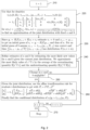
    • Fig. 2 shows a flow chart schematically illustrating another examples of the proposed approach; and
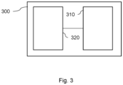
    • Fig. 3 shows a block diagram schematically illustrating an embodiment of the proposed apparatus.
  • A Bayes filter is a probabilistic algorithm used for state estimation in systems where uncertainty is present. It utilizes Bayes' theorem to update an estimate about a state of the system based on a new observation. The Bayes filter usually provides for two steps: prediction and update.
  • During the prediction step, the filter uses a dynamic model of the system to project the current state forward in time while taking into account an uncertainty of such prediction. Then in the update step, it combines the predicted state with the observation using Bayes' theorem to calculate a posterior estimate distribution while taking into account an uncertainty of the observation.
  • So, a key idea is to continuously refine the state estimate by iteratively incorporating new information while considering the uncertainty in both the observation and the system's dynamics. This makes Bayes filters particularly valuable in applications like robotics, localization, tracking, and sensor data fusion, where accurate state estimation is crucial in the presence of noisy or incomplete data.
  • However, current concepts of the Bayes filter struggle estimating the state accurately for observations including outliers. The present disclosure provides an approach tackling this problem.
  • In particular, the proposed approach provides for a method of a Bayes filter or smoother, as laid out in more detail below with reference to Fig. 1.
  • Fig. 1 shows a flow chart schematically illustrating a method 100 for a Bayes filter or smoother.
  • As can be seen from the flow chart, the method 100 comprises obtaining 110 an observation of an object state. The observation, e.g., is indicative of sensor data. So, for the observation, e.g., sensor data of one or more sensors is obtained. In embodiments, the observation may include the sensor data in a raw or processed form.
  • In practice, the proposed approach, e.g., is applied in an ADS for tracking traffic participants in an environment of a vehicle. In such applications, the sensor data, e.g., is sensor data from environmental sensors for determining a position and/or motion of traffic participants. Accordingly, the object state may indicate a position and/or motion and the observation may be indicative of a measurement (sensor data) of the position and/or motion.
  • The method 100 further provides for determining 120 the object state based on a joint Student's t-distribution. In doing so, determining the object state comprises approximating the joint Student's t-distribution of distributions for an object state estimate in a previous time step, a process noise, and the observation. The joint Student's t-distribution is based on a first and at least one second parameter and determining the object state comprises adapting the first parameter and the second parameter.
  • The joint Student's t-distribution exhibits fatter tails than other distributions such as a Gaussian distribution. So, the joint Student's t-distribution make the filter or smoother more robust to outliers in the observation.
  • So, it is proposed to use (independent) Student's t-distributions for the distributions of the object state estimate in the previous time step, the process noise, and the observation However, in doing so, one problem is that independent Student-t variables usually have no joint Student's t-distribution. So, the proposed approach suggests an approximation of the joint Student's t-distribution. According to the proposed approach, an approximation of the joint Student-t distribution focuses on high accuracy mainly around the unknown true state is suggested. This may automatically result in a different behavior for outliers than for well-behaved observations. In doing so, the proposed parametrization allows for a more accurate and resource efficient way to estimate the object state.
  • In practice, the Bayes filter often is a Kalman filter. Therefore, examples of the proposed approach are described in more detail in connection with applications in the Kalman filter. However, the skilled person will appreciate that the present approach may be also applied in other Bayes filters or smoothers.
  • Short Kalman filter proof
  • To clarify the parallels to the Student's t-distribution, Kalman filter equations shall be briefly discussed below. In particular, it is shown that these are direct consequences of the following three properties of multivariate normal distributions N μ Σ
    Figure imgb0008
    :
    • Affine transformations: If X N μ Σ
      Figure imgb0009
      and Y = AX + b then Y N A μ + b , A Σ A
      Figure imgb0010
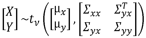
    • Conditional distributions: If X Y N μ x μ y Σ xx Σ yx T Σ yx Σ yy
      Figure imgb0011
      then Y | X N μ y + Σ yx Σ xx 1 X μ x , Σ yy Σ yy Σ xx 1 Σ yx T
      Figure imgb0012
    • Joint Independent Distributions: If X N μ x Σ x
      Figure imgb0013
      and Y N μ y Σ y
      Figure imgb0014
      are independent then they have a joint normal distribution X Y N μ x μ y Σ x 0 0 Σ y
      Figure imgb0015
      with A = I 0
      Figure imgb0016
      and b = 0, a direct consequence is:
    • Marginal Distributions: If X Y N μ x μ y Σ xx Σ yx T Σ yx Σ yy
      Figure imgb0017
      then X N μ x Σ xx
      Figure imgb0018
      .
  • For the Kalman (LTS) smoother, it is also useful to look at the following property for multivariate normal densities N x | μ , Σ
    Figure imgb0019
    : N x | x 0 , P 0 N y | Hx , R = N x y | x 0 Hx 0 , P 0 P 0 H T HP 0 HP 0 H T + R
    Figure imgb0020
  • This can be checked by deriving the marginal distribution of X and the conditional distribution of Y|X of the multivariate normal distribution on the right-hand side. Overall, we can now derive a Bayesian-type equation of the form p(x)p(ylx) = p(y)p(x|y) N ( x | x 0 , P 0 N y | Hx + a , R = N y | Hx _ 0 , H P _ 0 H T + R N x | x 0 + P 0 H T HP 0 H T + R 1 y Hx 0 , P 0 P 0 H T HP 0 H T + R 1 HP 0
    Figure imgb0021
  • Kalman filter equations
  • Assume x t 1 y 1 , , y t 1 = x t 1 y t 1 N μ t 1 P t 1
    Figure imgb0022
    , where µ t-1 denotes the expected value of the object state for the previous time step, and where only µ0 and P 0 are given, as well as x t = Fx t 1 + v t v t N 0 Q t
    Figure imgb0023
    y t = Hx t + e t e t N 0 R t
    Figure imgb0024
    where v and e are independent noise variables, F is a transition model, H is an observation model, Qt denotes a process covariance, Rt denotes an observation noise/uncertainty, yt is the observation at time or time step t, xt is the object state at time or time step t and x t-1 the object state of a previous time/time step. According to the affine transformation rule: x t 1 v t e t N μ t 1 0 0 P t 1 0 0 0 Q t 0 0 0 R t x t y t = F I 0 HF H I x t 1 v t e t N F μ t 1 HF μ t 1 FP t 1 F T + Q t FP t 1 F T H T + Q t H T HFP t 1 F T + HQ t HFP t 1 F T H T + HQ t H T + R t x t y t N μ t | t 1 H μ t | t 1 P t | t 1 P t | t 1 H T HP t | t 1 HP t | t 1 H T + R t ,
    Figure imgb0025
    where P denotes a covariance of an object state estimate, and where µ t|t-1 = Fµ t-1 and P t | t 1 = FP t 1 = FP 1 tF T + Q t
    Figure imgb0026
    . Thus, according to the above property of conditional distributions it follows that: x t | y t N ( μ t | t 1 + P t | t 1 H T HP t | t 1 H T + R t 1 y H μ t | t 1 ,
    Figure imgb0027
    P t | t 1 P t | t 1 H T HP t | t 1 H T + R t 1 HP t | t 1 ) x t | y t N μ t | t 1 + K t y H μ t | t 1 , I K t H P t | t 1
    Figure imgb0028
    with Kalman gain Kt = P t|t-1 HT (HP t|t-1 HT + Rt )-1
  • Parallels to the Student's t-distribution
  • A multivariate student-t distribution tv (µ,Σ) has the density t ν x | μ , Σ = Γ ν + p 2 Γ ν 2 ν p 2 π p 2 det Σ 1 + 1 ν x μ T Σ 1 x μ ν + p 2 ,
    Figure imgb0029
    where v is the degree of freedom discussed further down and p is the dimension of µ, i.e., Σ is a p × p matrix. Σ is the scale matrix, which can be seen as a scaled form of the covariance matrix.
  • So, the Student's t-distribution may be seen as a generalization of the multivariate normal distribution N μ Σ
    Figure imgb0030
    in the sense that a random variable X~tv (µ,Σ) can be seen as being Gaussian X N μ Φ
    Figure imgb0031
    with unknown precision/covariance matrix Φ. That is, Φ is in itself a random variable with Wishart distribution W(Σ/v,v).
  • The Wishart distribution is a positive-definite-matrix-valued distribution, which generalizes the one-dimensional concept of the gamma distribution and the χ-squared distribution with v degrees of freedom. As a more concrete definition, the Wishart distribution can be seen as the distribution of the empirical covariance matrix of samples G i N 0 Σ
    Figure imgb0032
    , i.e., 1 ν i = 1 ν G i G i T W Σ ν ν .
    Figure imgb0033
  • It already becomes apparent, that if v becomes large, then 1 ν i = 1 ν G i G i T
    Figure imgb0034
    converges to Z in probability. Thus, we can expect tv (µ, Σ) to converge to N μ Σ
    Figure imgb0035
    . In practice, for v > 30, these distributions can be treated as superficially the same.
  • The Student's t-distribution inherits a few properties from the multivariate normal distribution:
    1. 1. Affine Transformations: If X ~ tv (µ, Σ) and Y = AX + b then Y ~ tv (A µ + b, AΣAT )
    2. 2. Conditional Distributions: If X Y t ν μ x μ y Σ xx Σ yx T Σ yx Σ yy
      Figure imgb0036
      then Y | X t ν + p z μ y + Σ yx Σ xx 1 X μ x , ν + X μ x T Σ xx 1 X μ x ν + p x Σ yy Σ yx Σ yx T .
      Figure imgb0037
  • Note that the parameterization of these distributions is the same as the parameterization in the multivariate normal case, with the two exceptions. Firstly, the degrees of freedom increase with conditioning, i.e. conditioned Student's t-distribution are closer to normal distributions. And secondly, the covariance matrix of the conditioned matrix is weighted by the squared Mahalanobis distance X μ x T Σ xx 1 X μ x
    Figure imgb0038
    of the observation X to the expectation µ x in such a way that the covariance matrix can at most shrink by a factor of ν ν + p z
    Figure imgb0039
    but can increase to capture the degree of uncertainty an outlier brings.
  • However, while the marginal distributions can again be concluded from the property under affine transformations, finding a joint density for two independent Student's t-distribution variables is more elaborate.
  • Suppose X ~ tχ x, Σx ) and Y - tω y, Σy ), then the intuitive thing would be to expect that X Y t ν μ x μ y Σ x 0 0 Σ y
    Figure imgb0040
    for some degrees of freedom χ. This is the case when X|Y = X holds but X | Y t ν + p y μ x , ν + Y μ y T Σ y 1 Y μ y ν + p y Σ x ,
    Figure imgb0041
    implies that if Y is an outlier, then X is more likely also an outlier. In particular, two random variables which are jointly distributed are not independent.
  • The expected Mahalanobis distance
  • Let's look at the expected value of Y μ y T Σ y 1 Y μ y
    Figure imgb0042
    where Y~tv y, Σy ) is the marginalized distribution. Let Σy = LLT, then for = L -1(Y - µ y ) it follows that Y μ y T Σ y 1 Y μ Y = Y ^ T Y ^
    Figure imgb0043
    and ~tv (L -1µ y - L -1µ y, L -1 ΣyL -1) = tv (0, Ipy ). Now note that Tr(yyT ) = Σiyiyi = yTy. Thus, E Y μ y T Σ y 1 Y μ y = E Y ^ T Y ^ = E Tr Y ^ Y ^ T = E i = 1 p y Y ^ i 2 = i = 1 p y E Y ^ i 2 = i = 1 p y Cov Y ^ ii = Tr Cov Y ^ .
    Figure imgb0044
  • Note that the covariance matrix of Ŷ~tv (0, Ipy ) is ν ν 2 p y
    Figure imgb0045
    , if v > 2 and undefined (i.e., ∞) otherwise. Thus E Y μ y T Σ y 1 Y μ y = ν ν 2 p y
    Figure imgb0046
    . More generally, 1 p y Y μ y T Σ y 1 Y μ y F p y ν
    Figure imgb0047
    , wherein F is Snedecor's F-distribution.
  • Note that by the conditioning property, it holds that t ν x t 1 v t e t | μ t 1 0 0 , a t P t 1 0 0 0 a t b t Q t 0 0 0 R t = t ν e t | o , R t t ν + p y x t 1 v t | μ t 1 0 , ν + e t T R t 1 e t ν + p y a t P t 1 0 0 bQ t = t ν e t | 0 , R t t ν + p y x t 1 | μ t 1 , ν + e t T R t 1 e t ν + p y a t P t 1 t ν + p y + p z v t | 0 , ν + p y + x t 1 μ t 1 T ν + e t T R t 1 e t ν + p y a t P t 1 1 x t 1 μ t 1 ν + p y + p x ν + e t T R t 1 e t ν + p y a t b t Q t
    Figure imgb0048
  • That is, if a t = ν + p y ν + e t T R t 1 e t
    Figure imgb0049
    and b t = ν + p y + p x ν + p y + x t 1 μ t 1 T P t 1 1 ( x t 1 μ t 1
    Figure imgb0050
    are known then one have found an approximation of the joint Student's t-distribution t v-py (x t-1 t-1, P t-1) · t v+py+px (vt |0, Qt ) · tv (et |0, Rt ) which is approximately exact (i.e., indicates the object state and noises approximately) in a small region around [x t-1 , vt, et ] T. Note that one actually does not need to know the actual values of x t-1 and et for the approximation but only their Mahalanobis distance, as laid out in more detail below.
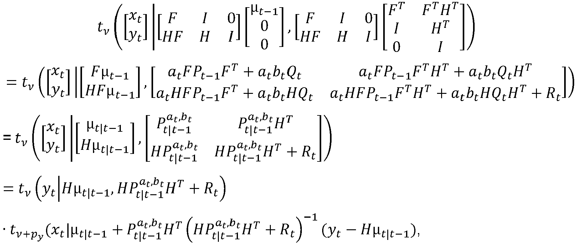
  • With this approximation, it is proposed to perform the following steps t ν x t y t | F I 0 HF H I μ t 1 0 0 , F I 0 HF H I F T F T H T I H T 0 I = t ν x t y t | F μ t 1 HF μ t 1 , a t FP t 1 F T + a t b t Q t a t FP t 1 F T H T + a t b t Q t H T a t HFP t 1 F T + a t b t HQ t a t HFP t 1 F T H T + a t b t HQ t H T + R t = t ν x t y t | μ t | t 1 H μ t | t 1 , P t | t 1 a t , b t P t | t 1 a t , b t H T HP t | t 1 a t , b t HP t | t 1 a t , b t H T + R t = t ν y t | H μ t | t 1 , HP t | t 1 a t , b t H T + R t t ν + p y ( x t | μ t | t 1 + P t | t 1 a t , b t H T HP t | t 1 a t , b t H T + R t 1 y t H μ t | t 1 ,
    Figure imgb0051
    ν + y t H μ t | t 1 T ( H ( P t | t 1 a t , b t H T HP t | t 1 a t , b t H T + R t 1 y t H μ t | t 1 ν + p y P t | t 1 a t , b t P t | t 1 a t , b t H T HP t | t 1 a t , b t H T + R t 1 HP t | t 1 a t , b t )
    Figure imgb0052
  • Thus, the proposed posterior distribution is t ν + p y x t | μ t | t 1 + K y t H μ t | t 1 , Δ I KH P t | t 1 a t , b t
    Figure imgb0053
    with P t | t 1 a t , b t = a t FP t 1 F T + a t b t Q t , K = P t | t 1 a t , b t H T HP t | t 1 a t , b t H T + R t 1
    Figure imgb0054
    Δ = ν + y t H μ t | t 1 T HP t | t 1 a t , b t H T + R t 1 y t H μ t | t 1 ν + p y .
    Figure imgb0055
  • Note that both the distributions for x t-1 and xt have v + py degrees of freedom. Thus, the filter will not decay to the standard Kalman filter.
  • Now, according to the proposed approach, at and bt are estimated/approximated to solve the joint Student's t-distribution.
  • Estimating at
  • For this, one can find a corresponding solution for e t T R t 1 e t
    Figure imgb0056
    and (x t-1 - μ t 1 ) T P t 1 1 x t 1 μ t 1
    Figure imgb0057
    . For at and estimating e t T R t 1 e t
    Figure imgb0058
    one has a priori only the assumed distribution of et . However, one can exploit information carried by the observed yt = Hxt + et to get a more informed state of et. For that one can find the distribution of et |yt in the same way xt |yt was found. t ν y t e t | HF H I 0 0 I μ t 1 0 0 , HF H I 0 0 I a t P t 1 0 0 0 a t b t Q t 0 0 0 R t F T H T 0 H T 0 I I = t ν y t e t | HF μ t 1 0 , a t HPF t 1 F T H T + a t b t HQ t H T + R t R t R t R t = t ν y t e t | HF μ t 1 0 , S t a t , b t R t R t R t = t ν y t | HF μ t 1 , S t a t , b t t ν + p y e t | R t S t a t , b t 1 y t HF μ t 1 , Δ R t R t S t a t , b t 1 R t
    Figure imgb0059
  • Thus et |yt has a Student's t-distribution with v + py degrees of freedom, mean m = R t S t a t , b t 1 y t HF μ t 1
    Figure imgb0060
    and covariance matrix ν + p y ν + p y 2 Δ R t R t S t a t , b t R t 1
    Figure imgb0061
    . Using this distribution one is able to find the distribution of e t T R t 1 e t | y t , a t , b t
    Figure imgb0062
    , one might call p e t T R t 1 e t | y t , a t , b t
    Figure imgb0063
    and find the value of e t T R t 1 e t
    Figure imgb0064
    which maximizes this likelihood. However, the distribution of e t T R t 1 e t | y t , a t , b t
    Figure imgb0065
    is a generalized non-central F-distribution for which the density is analytically described as a series and thus finding the maximum might be too much computational effort.
  • Thus, it is proposed to approximate the likelihood-maximizing value. For this, note on the one hand that approximating the most likely e t T R t 1 e t | y t , a t , b t
    Figure imgb0066
    by the estimate m T R t 1 m
    Figure imgb0067
    , where m = E e t | y t , a t , b t
    Figure imgb0068
    underestimates the target value (see, e.g., the extreme case m = 0, where the most likely Mahalanobis distance would be approximated by 0). And note that on the other hand, E e t T R t 1 e t | y t , a t , b t
    Figure imgb0069
    overestimates the most likely Mahalanobis distance due to the heavy tail and asymmetry of the distribution of e t T R t 1 e t | y t , a t , b t
    Figure imgb0070
    by the average of these over-/underestimating approximations. Thus overall, it is proposed to define at as a fixed point of the equation a t = ν + p y ν + E e t T R t 1 e t | y t , a t , b t + m T R t 1 m 2
    Figure imgb0071
    with the initial guess a t 0 = ν + p y ν + y t HF μ t 1 T R t 1 y t HF μ t 1
    Figure imgb0072
    .
  • Now let = (et |yt, at, bt ) - m then since E e ˜ = 0
    Figure imgb0073
    E e t T R t 1 e t | y t , a t , b t = E e ˜ + m T R t 1 e ˜ + m = E e t T R t 1 e t + m T R t 1 m
    Figure imgb0074
  • Furthermore, e = R t 1 2 e ˜
    Figure imgb0075
    has distribution t ν + p y e | 0 , Δ I R t 1 2 S t a t , b t R t 1 2 1
    Figure imgb0076
    and by the expression of the Mahalanobis distance developed above E e t T R t 1 e t | y t , a t , b t = E e T e + m T R t 1 m = ν + p y ν + p y 2 Δ Tr I R t 1 2 S t a t , b t 1 R t 1 2 + y t HF μ t 1 T S t a t , b t 1 R t R t 1 R t S t a t , b t 1 y t HF μ t 1 = ν + y t H μ t | t 1 T r t a t , b t ) ν + p y 2 p y Tr R t S t a t , b t 1 + r t a t , b t T R t r t a t , b t
    Figure imgb0077
    for r t a t , b t = S t a t , b t y t HF μ t 1 1
    Figure imgb0078
    . Also note that the trace is easily computable through elementwise multiplication ⊙ Tr R t S t a t , b t 1 = i = 1 p y R t S t a t , b t 1 ii = i = 1 p y j = 1 p y R t ij S t a t , b t 1 ji = iJ R t T S t a t , b t 1 ij
    Figure imgb0079
  • Estimating bt
  • It is proposed to perform the same steps to get an approximation of (x t-1 - µ t-1) T (P t-1)-1(x t-1 - µ t-1). t ν x t 1 y t | I 0 0 HF H I μ t 1 0 0 , I 0 0 HF H I a t P t 1 0 0 0 a t b t Q t 0 0 0 R t I F T H T 0 H T 0 I = t ν x t 1 y t | μ t 1 HF μ t 1 , a t P t 1 a t P t 1 F T H T a t HFP t 1 a t HFP t 1 F T H T + a t b t HQ t H T + R t = t ν x t 1 y t | μ t 1 HF μ t 1 , a t P t 1 a t P t 1 F T H T a t HFP t 1 S t a t , b t = t ν y t | HF μ t 1 , S t a t , b t t ν + p y ( x t 1 | μ t 1 + a t P t 1 F T H T S t a t , b t 1 y t HF μ t 1 ,
    Figure imgb0080
    Δa t P t 1 a t P t 1 F T H T S t a t , b t 1 HFP t 1 ) .
    Figure imgb0081
    For m = a t P t 1 F T H T S t a t , b t 1 y t HFμ t 1
    Figure imgb0082
    and z = P 1 2 x t 1 | y t μ t 1 m
    Figure imgb0083
    . Then z t ν + p y 0 , Δa t I a t P t 1 1 2 F T H T S t a t , b t 1 HFP t 1 1 2
    Figure imgb0084
    and E x t 1 μ t 1 T P t 1 1 x t 1 μ t 1 | y t = E P 1 2 z + m T P t 1 1 P 1 2 z + m = E z T z + m T P t 1 1 m = ν + p y ν + p y 2 Δa t Tr I a t P t 1 1 2 F T H T S t a t , b t 1 HFP t 1 1 2 + a t 2 y t HF μ t 1 T S t a t , b t 1 HFP t 1 P t 1 1 P t 1 F T H T S t a t , b t 1 y t HF μ t 1 = ν + y t H μ t | t 1 T S t a t , b t 1 y t H μ t | t 1 ν + p y 2 a t p y a t Tr HFP t 1 F T H T S t a t , b t 1 + a t 2 y t HF μ t 1 T S t a t , b t 1 HFP t 1 F T H T S t a t , b t 1 y t HF μ t 1 = ν + y t H μ t 1 T r t a t , b t ν + p y 2 a t p y a t HFP t 1 F T H T S t a t , b t 1 + a t 2 r t a t , b t T HFP t 1 F T H T r t a t , b t
    Figure imgb0085
    again with S t a t , b t = a t HFP t 1 F T H T + a t b t HQ t H T + R t
    Figure imgb0086
    and r t a t , b t = S t a t , b t 1 ( y t
    Figure imgb0087
    HFµ t-1).
  • In particular, note that HFF t-1 FTHT and HQtHT can be pre-computed and each iteration of finding at and bt may only require a single py × py matrix inversion, no additional matrix multiplication and otherwise on matrix-vector and component-wise matrix-multiplications (which are of the order of p y 2
    Figure imgb0088
    and basically free).
  • For an initial guess of bt it is proposed to ignore the observation yt and assume x t 1 t ν + p y μ t 1 P t 1 ,
    Figure imgb0089
    x t 1 μ t 1 T P t 1 1 x t 1 μ t 1 = z T z with z t ν + p y 0 I .
    Figure imgb0090
  • And as described before, it is proposed that if some z~t v+py (0, I) has standard normal Student's t-distribution, then 1 p x z T z F p x , ν + p y
    Figure imgb0091
    . And the density of this F-distribution maximizes at its mode p x 2 p x ν + p y ν + p y + 2
    Figure imgb0092
    if px > 2 else 0. Thus, the initial guess of bt is b t 0 = ν + p y + p x ν + p y + max p x 2,0 ν + p y ν + p y + 2 .
    Figure imgb0093
  • Estimating the distribution of x t-1 might appear more intuitive using y t-1. However, note that the proposed estimate of x t-1 is already conditioned on y t-1.
  • The proposed approach, e.g., is implemented in an iterative process, e.g., for tracking an object over time T for multiple timesteps t = 1, ..., T, as laid out in more detail with reference to Fig. 2.
  • As can be seen from the flow chart, e.g., in a first step 210, a first time step t is determined, e.g. t = 1.
  • Then, in a second step 220, the joint Student's t-distribution for the current time step is determined to find an approximation of it for values of the parameters a(et ) and b(et, xt ).
  • In a following step 230, then, an initial guess for the parameters is made, as laid out above in more detail. Further, in a next step 240, the parameters are refined.
  • This may be done iteratively until the parameters do not change significantly anymore in doing so. For this, the change of the refinement is checked in another step 250. In order to do so, the change, e.g., is compared to a predefined threshold. In the case, the refinement changes the parameters significantly, they are refined further. If they do not change significantly, the parameters are used to solve the joint Student's t-distribution to determine the object state.
  • In the present example, it may be desired to stop the process after the predefined period T. To this end, another step 270 provides for checking if t < T and to stop if t is greater than T. In other embodiments, the process may be executed continuously. In such embodiments, step 270 may be omitted.
  • In practice, the proposed approach, e.g., may be implemented in a computer program to execute steps of the method using a computer.
  • An exemplary code of such a computer program could include instructions as follows (pseudo code instructions bold-faced):
    Given timesteps t = 1, ... , T, linear state-transmission models F t n × m
    Figure imgb0094
    , linear observation models H t m × n
    Figure imgb0095
    , process covariances Q t n × n
    Figure imgb0096
    , observation covariances R t m × m
    Figure imgb0097
    , degrees of freedom v and observations y t m
    Figure imgb0098
    , as well as an initial guess of the true state by mean µ0 and covariance P 0.
  • Assume that a sequence of true states and noisy measurements is a Markov-Chain with additive Student's t-distributed noise, e.g., x t = F t x t 1 + v t v t t ν + n + m 0 Q t
    Figure imgb0099
    y t = H t x t + e t e t t ν 0 R t
    Figure imgb0100
  • Results in estimations of the true states xt by Student's t-distributions t v+m t , Pt ) only using observations y 1, ... , yt for each t.
    for t = 1, ...T do P ^ t = FP t 1 F T , P ^ t H = H P ^ t H T , Q t H = HQ t H T
    Figure imgb0101
    μ ^ t F μ t 1 , r t = y t H μ ^ t , i = 0
    Figure imgb0102
    a 0 = ν + m ν + r t T R t 1 r t , b 0 = ν + m + n ν + m + max p x 2,0 ν + m ν + m + 2
    Figure imgb0103
    (initial guess for a and b) do (for Fixpoint iteration of a and b to approximate the joint Student's t-distribution) S = a i P ^ t H + a i b i Q t H + R t 1 , s = Sr t
    Figure imgb0104
    c = ν + r t T s ν + m 2 , i = i + 1
    Figure imgb0105
    a i = ν + m ν + c m i , j m R t ij S ij / 2 + s T R t s
    Figure imgb0106
    b i = ν + m + n ν + m + c a i 1 m a i 1 i , j m R t ij S ij 1 2 + a i 1 2 s T P ^ t H s )
    Figure imgb0107
    while a i a i 1 a i + a i 1 + b i b i 1 b i + b i 1 > 10 4
    Figure imgb0108
    (or any other arbitrary/appropriate threshold) P t | t 1 = a i 1 P ^ t + b i 1 Q t
    Figure imgb0109
    μ t = μ ^ t + P t | t 1 H T s
    Figure imgb0110
    P t = c ν + m 2 ν + m P t | t 1 P t | t 1 H T SHP t | t 1
    Figure imgb0111
    end for
  • Analogously, features and aspects of the described examples can be transferred to data smoothers, e.g., fixed-interval smoothers for data.
  • As the skilled person will appreciate, the described examples may be applied in various applications of Bayes filter or smoothers.
  • Bayes filter, e.g., are used in sensor data fusion where sensor data of two or more sensor is fused. Accordingly, the proposed approach may be applied for fusing sensor data of a first and at least one second sensor. However, applications of the proposed approach are not only limited to sensor data fusion but may also include other use cases.
  • The Student's-t smoother
  • Analogously to the above description, the proposed smoother uses a joint Student's t-distribution of two subsequent object state estimations xt and x t+1 of a current time step t and a subsequent time step t + 1. The joint Student's t-distribution can be derived by: t ν + p y x t | y 1 , , y t | μ t , P t t ν + p y + p x v t + 1 | 0 Q t + 1 = t ν + p y x t v t + 1 | y 1 , , y t | μ t 0 , P t 0 0 b t + 1 Q t + 1
    Figure imgb0112
    Where b t + 1 is again ν + p y + p x ν + p y + x t μ t T P t 1 x t μ t x t x t + 1 | y 1 , , y t = I 0 F I x t v t + 1 | y 1 , , y t + 1 t ν + p y μ t F μ t P t P t F T FP t FP t F T + b t + 1 Q t + 1 x t | x t + 1 , y 1 , , y t t ν + p y + p x μ t + P t F T FP t F T + b t + 1 Q t + 1 1 x t + 1 F μ t ,
    Figure imgb0113
    Δ P t P t F T FP t F T + b t + 1 Q t + 1 1 FP t
    Figure imgb0114
    Δ = ν + p y + x t + 1 F μ t T FP t F T + b t + 1 Q t + 1 1 x t + 1 F μ t ν + p y + p x
    Figure imgb0115
  • The distribution of xt |y 1, ... , yT is now derived from the joint Student's t-distribution of [xt , x t+1] T |y 1, ... , yT and the marginal distribution of xt |y 1 , ... yT. Note that xt |x t+1 , y 1 , ... , yT = xt |x t+1 , y 1 , ... , yt since the additional observations y t+1 , ... , yT do not provide information not already present in x t+1. Together with the given distribution of x t + 1 | y 1 , , y T t ν + p y μ t + 1 T P t + 1 T
    Figure imgb0116
    and J = PtFT (FPtFT + btQ t+1)-1 t ν + p y + p x x t | x t + 1 , y 1 , , y T | μ T + J x t + 1 F μ t , Δ P t JFP t t ν + p y x t + 1 | y 1 , , y T | μ t + 1 T , P t + 1 T = t ν + p y x t x t + 1 | y 1 , , y T | m 1 μ t + 1 T , Σ 11 Σ 12 Σ 12 T P t + 1 T = t ν + p y + p x x t | x t + 1 , y 1 , , y T | m 1 + Σ 12 P t + 1 T 1 x t + 1 μ t + 1 T , 1 b t + 2 T Σ 11 Σ 12 P t + 1 T 1 Σ 12 T t ν + p y x t + 1 | y 1 , , y T | μ t + 1 T , P t + 1 T ,
    Figure imgb0117
    wherein 1 b t + 2 T = ν + p y + x t + 1 μ t + 1 T T P t + 1 T 1 x t + 1 μ t + 1 T ν + p y + p x
    Figure imgb0118
  • For solving the joint Student's t-distribution, m 1, Σ 11, and Σ 12 can be found by comparison of variables: Jx t + 1 = Σ 12 P t + 1 T 1 x t + 1 Σ 12 = JP t + 1
    Figure imgb0119
    μ t JF μ t = m 1 Σ 12 P t + 1 T 1 μ t + 1 T m 1 = μ t + J μ t + 1 T F μ t
    Figure imgb0120
    Δ p t JFP t ) = 1 b t + 2 T Σ 11 Σ 12 P t + 1 T 1 Σ 12 T
    Figure imgb0121
    Σ 11 = Δb t + 2 T P t + JP t + 1 T J T Δb t + 2 T JFP t = Δb t + 2 T P t + J P t + 1 T Δb t + 2 T FP t F T + b t Q t + 1 J T ,
    Figure imgb0122
    where FPt = (FPtFT + btQ t+1)JT . Thus, by marginalizing the above joint Student's t-distribution one can obtain x t | y 1 , , y T t ν + p y μ t + J μ t + 1 T F μ t , Δb t + 2 T P t + J P t + 1 T Δb t + 2 T FP t F T + b t Q t + 1 J T
    Figure imgb0123
  • Further, it is proposed to approximate b t + 2 T
    Figure imgb0124
    and b t+1 using the same approach as in the filter. Firstly, μ t + 1 T
    Figure imgb0125
    and P t + 1 T
    Figure imgb0126
    already incorporate all available information y 1,...,yT , therefore we will, similar to the initial guess of b t + 2 T
    Figure imgb0127
    , assume that x t + 1 μ t + 1 T T P t + 1 T 1 x t + 1 μ t + 1 T p x F p x , ν + p y
    Figure imgb0128
    . Thus our approximation becomes b t + 2 T = ν + p y + p x ν + p y + max p x 2,0 ν + p y ν + p y 2
    Figure imgb0129
  • For b t+1 we can first use the value found during the filtering process as initial guess and then use the found distribution of xt |y 1, ... , yT for a more informed estimate of (xt - µ t ) TPt -1(xt - µ t ) in the same way we found b t+1 from xt |y 1, ... , y t+1 .
  • The proposed approach may be also implemented in an apparatus, as laid out in more detail with reference to Fig. 3.
  • Fig. 3 shows a block diagram schematically illustrating an exemplary embodiment of such an apparatus 300.
  • In embodiments, the one or more interfaces 310 may comprise wired and/or wireless interfaces for transmitting and/or receiving communication signals in connection with the execution of the proposed concept. In practice, the interfaces, e.g., comprise pins, wires, antennas, and/or the like. As well, the interfaces may comprise means for (analog and/or digital) signal or data processing in connection with the communication, e.g., filters, samples, analog-to-digital converters, signal acquisition and/or reconstruction means as well as signal amplifiers, compressors and/or any encryption/decryption means.
  • The data processing circuit 320 may correspond to or comprise any type of programable hardware. So, examples of the data processing circuit 320, e.g., comprise a memory, microcontroller, field programable gate arrays, one or more central, and/or graphical processing units. To execute the proposed method, the data processing circuit 320 may be configured to access or retrieve an appropriate computer program for the execution of the proposed method from a memory of the data processing circuit 320 or a separate memory which is communicatively coupled to the data processing circuit 320.
  • In practice, the proposed apparatus may be installed on a vehicle. So, embodiments may also provide a vehicle comprising the proposed apparatus. In implementations, the apparatus, e.g., is part or a component of the ADS.
  • In the foregoing description, various features are grouped together in examples for the purpose of streamlining the disclosure. This method of disclosure is not to be interpreted as reflecting an intention that the claimed examples require more features than are expressly recited in each claim. Rather, as the following claims reflect, subject matter may lie in less than all features of a single disclosed example. Thus, the following claims are hereby incorporated into the description, where each claim may stand on its own as a separate example. While each claim may stand on its own as a separate example, it is to be noted that, although a dependent claim may refer in the claims to a specific combination with one or more other claims, other examples may also include a combination of the dependent claim with the subject matter of each other dependent claim or a combination of each feature with other dependent or independent claims. Such combinations are proposed herein unless it is stated that a specific combination is not intended. Furthermore, it is intended to include also features of a claim to any other independent claim even if this claim is not directly made dependent to the independent claim.
  • Although specific embodiments have been illustrated and described herein, it will be appreciated by those of ordinary skill in the art that a variety of alternate and/or equivalent implementations may be substituted for the specific embodiments shown and described without departing from the scope of the present embodiments. This application is intended to cover any adaptations or variations of the specific embodiments discussed herein. Therefore, it is intended that the embodiments be limited only by the claims and the equivalents thereof.

Claims (13)

  1. A method (100) for a Bayes filter or smoother, the method (100) comprising:
    obtaining (110) an observation of an object state;
    determining (120) the object state based on a joint Student's t-distribution, wherein determining the object state comprises approximating the joint Student's t-distribution of distributions for an object state estimate in a previous time step, a process noise, and the observation, wherein the joint Student's t-distribution is based on a first and at least one second parameter, and wherein determining the object state comprises adapting the first parameter and the second parameter.
  2. The method (100) of claim 1, wherein the first parameter is a parameter for the object state estimate and the process noise and the second parameter is a parameter for the process noise.
  3. The method (100) of claim 1 or 2, wherein the joint Student's t-distribution is: t ν x t 1 v t e t | μ t 1 0 0 , a t P t 1 0 0 0 a t b t Q t 0 0 0 R t
    Figure imgb0130
    , wherein Qt represents a process covariance for the process noise, P t-1 represents a covariance of the object state estimate, at represents the first parameter, bt represents the second parameter, x t-1 represents the object state estimate, vt represents the process noise, et represents an observation uncertainty, µ t-1 represents the mean state for the object state estimate at the previous time step, and Rt represents a covariance for the observation uncertainty.
  4. The method (100) of any one of the preceding claims, wherein determining the state of the object based on a joint Student's t-distribution comprises solving the joint Student's t-distribution based on an approximation for the first and the second parameter.
  5. The method (100) of claim 4, wherein the approximation comprises adjusting the first and the second parameter based on the observation and one or more previous approximations.
  6. The method (100) of claim 4 or 5, wherein the approximation comprises:
    obtaining initial guess for the first and the second parameter, wherein the initial guess for the first parameter is a t 0 = ν + p y ν + y t HFμ t 1 T R t 1 y t HFμ t 1
    Figure imgb0131
    , and the initial guess for the second parameter is b t 0 = ν + p y + p x ν + p y + max p x 2,0 a t 0 ν + p y ν + p y + 2
    Figure imgb0132
    , wherein v, py, and px represent degrees of freedom, yt represents a state observation indicative of the observation, Rt represents a covariance for the observation uncertainty, µ t-1 represents the mean state for the state estimate at the previous time step, H represents an observation model, and F represents a transition model; and
    refining the initial guess for the first and the second parameter.
  7. The method (100) of any one of the preceding claims, wherein the observation is indicative of sensor data of a first and at least one second sensor, and wherein the method (100) is applied for fusing the sensor data of the first and the second sensor.
  8. The method (100) of any one of the preceding claims, wherein the method (100) is for the use of a vehicle, and wherein the observation is indicative of sensor data from one or more sensors of the vehicle.
  9. The method (100) of any one of the preceding claims, wherein the object is a traffic participant.
  10. The method (100) of claim 9, wherein the state indicates a position and/or motion of the traffic participant.
  11. A computer program comprising instructions which, when the computer program is executed by a computer, cause the computer to carry out the method (100) of any one of the preceding claims.
  12. An apparatus (300) comprising:
    one or more interfaces (310) for communication; and
    a data processing circuit (320) configured to execute the method (100) of any one of the claims 1 to 10.
  13. A vehicle comprising the apparatus (300) of claim 12.
EP23197459.3A 2023-09-14 2023-09-14 Computer program, apparatus, vehicle, and method for a bayes filter or smoother Pending EP4524778A1 (en)

Priority Applications (2)

Application Number Priority Date Filing Date Title
EP23197459.3A EP4524778A1 (en) 2023-09-14 2023-09-14 Computer program, apparatus, vehicle, and method for a bayes filter or smoother
PCT/EP2024/075096 WO2025056455A1 (en) 2023-09-14 2024-09-09 Computer program, apparatus, vehicle, and method for a bayes filter or smoother

Applications Claiming Priority (1)

Application Number Priority Date Filing Date Title
EP23197459.3A EP4524778A1 (en) 2023-09-14 2023-09-14 Computer program, apparatus, vehicle, and method for a bayes filter or smoother

Publications (1)

Publication Number Publication Date
EP4524778A1 true EP4524778A1 (en) 2025-03-19

Family

ID=88093811

Family Applications (1)

Application Number Title Priority Date Filing Date
EP23197459.3A Pending EP4524778A1 (en) 2023-09-14 2023-09-14 Computer program, apparatus, vehicle, and method for a bayes filter or smoother

Country Status (2)

Country Link
EP (1) EP4524778A1 (en)
WO (1) WO2025056455A1 (en)

Non-Patent Citations (2)

* Cited by examiner, † Cited by third party
Title
BERNTORP KARL ET AL: "Approximate Noise-Adaptive Filtering Using Student-t Distributions", 2018 ANNUAL AMERICAN CONTROL CONFERENCE (ACC), AACC, 27 June 2018 (2018-06-27), pages 2745 - 2750, XP033387117, DOI: 10.23919/ACC.2018.8430902 *
HUANG YULONG ET AL: "A Novel Robust Student's t-Based Kalman Filter", IEEE TRANSACTIONS ON AEROSPACE AND ELECTRONIC SYSTEMS, IEEE SERVICE CENTER, PISCATAWAY, NJ, US, vol. 53, no. 3, 7 June 2017 (2017-06-07), pages 1545 - 1554, XP011651979, ISSN: 0018-9251, [retrieved on 20170607], DOI: 10.1109/TAES.2017.2651684 *

Also Published As

Publication number Publication date
WO2025056455A1 (en) 2025-03-20

Similar Documents

Publication Publication Date Title
Gao et al. Long short-term memory-based deep recurrent neural networks for target tracking
Ravindran et al. Camera, LiDAR, and radar sensor fusion based on Bayesian neural network (CLR-BNN)
JP5539680B2 (en) Object tracking using linear features
O'Callaghan et al. Contextual occupancy maps using Gaussian processes
Beard et al. Sensor control for multi-target tracking using Cauchy-Schwarz divergence
US20100262286A1 (en) Decision making mechanism, method, module, and robot configured to decide on at least one prospective action of the robot
Mullane et al. A random set formulation for Bayesian SLAM
Houssineau A linear algorithm for multi-target tracking in the context of possibility theory
Petetin et al. Bayesian multi-object filtering for pairwise Markov chains
Meier et al. Using the condensation algorithm to implement tracking for mobile robots
Leung et al. Relating random vector and random finite set estimation in navigation, mapping, and tracking
Xia et al. Extended object tracking with automotive radar using learned structural measurement model
US12528483B2 (en) Method, electronic device and medium for target state estimation
Truzman et al. Outlier-insensitive Kalman filtering: Theory and applications
CN117557810A (en) Research on an integrated detection and tracking algorithm based on attention mechanism and scale fusion
Wei et al. Bayesian Multiobject Tracking With Neural-Enhanced Motion and Measurement Models
EP2275993A2 (en) Method for estimating the visibility of features on surfaces of object instances in multi-object scenes and method for perception planning in multi-object scenes
EP4524778A1 (en) Computer program, apparatus, vehicle, and method for a bayes filter or smoother
WO2022194899A1 (en) Filtering noisy observations
Urteaga et al. Sequential estimation of hidden ARMA processes by particle filtering—Part I
Wu et al. In situ evaluation of tracking algorithms using time reversed chains
Marković et al. Direction-only tracking of moving objects on the unit sphere via probabilistic data association
Reith-Braun et al. Approximate first-passage time distributions for Gaussian motion and transportation models
Chang et al. Confidence level estimation in multi-target classification problems
Petrucci Gaussian mixture reduction for Bayesian target tracking in clutter

Legal Events

Date Code Title Description
PUAI Public reference made under article 153(3) epc to a published international application that has entered the european phase

Free format text: ORIGINAL CODE: 0009012

STAA Information on the status of an ep patent application or granted ep patent

Free format text: STATUS: THE APPLICATION HAS BEEN PUBLISHED

AK Designated contracting states

Kind code of ref document: A1

Designated state(s): AL AT BE BG CH CY CZ DE DK EE ES FI FR GB GR HR HU IE IS IT LI LT LU LV MC ME MK MT NL NO PL PT RO RS SE SI SK SM TR

STAA Information on the status of an ep patent application or granted ep patent

Free format text: STATUS: REQUEST FOR EXAMINATION WAS MADE

17P Request for examination filed

Effective date: 20250919

RAP3 Party data changed (applicant data changed or rights of an application transferred)

Owner name: AUMOVIO GERMANY GMBH