EP4398130A1 - Data processing device, control system, data processing method, and program - Google Patents
Data processing device, control system, data processing method, and program Download PDFInfo
- Publication number
- EP4398130A1 EP4398130A1 EP22864714.5A EP22864714A EP4398130A1 EP 4398130 A1 EP4398130 A1 EP 4398130A1 EP 22864714 A EP22864714 A EP 22864714A EP 4398130 A1 EP4398130 A1 EP 4398130A1
- Authority
- EP
- European Patent Office
- Prior art keywords
- matrix
- equation
- data
- control
- holds
- Prior art date
- Legal status (The legal status is an assumption and is not a legal conclusion. Google has not performed a legal analysis and makes no representation as to the accuracy of the status listed.)
- Pending
Links
Images









Classifications
-
- G—PHYSICS
- G06—COMPUTING OR CALCULATING; COUNTING
- G06F—ELECTRIC DIGITAL DATA PROCESSING
- G06F17/00—Digital computing or data processing equipment or methods, specially adapted for specific functions
- G06F17/10—Complex mathematical operations
-
- G—PHYSICS
- G06—COMPUTING OR CALCULATING; COUNTING
- G06F—ELECTRIC DIGITAL DATA PROCESSING
- G06F17/00—Digital computing or data processing equipment or methods, specially adapted for specific functions
- G06F17/10—Complex mathematical operations
- G06F17/16—Matrix or vector computation, e.g. matrix-matrix or matrix-vector multiplication, matrix factorization
-
- G—PHYSICS
- G05—CONTROLLING; REGULATING
- G05B—CONTROL OR REGULATING SYSTEMS IN GENERAL; FUNCTIONAL ELEMENTS OF SUCH SYSTEMS; MONITORING OR TESTING ARRANGEMENTS FOR SUCH SYSTEMS OR ELEMENTS
- G05B13/00—Adaptive control systems, i.e. systems automatically adjusting themselves to have a performance which is optimum according to some preassigned criterion
- G05B13/02—Adaptive control systems, i.e. systems automatically adjusting themselves to have a performance which is optimum according to some preassigned criterion electric
Definitions
- a controllability Gramian is known as an indicator for controllability of a system, see, for example, Non-Patent Document 1-6. Whether a system is controllable can be determined by whether the controllability Gramian is regular. Furthermore, the magnitude of the eigenvalues of the controllability Gramian quantitatively indicates the degree of influence of the input on the state.
- a Controllability Gramian can be easily calculated if a mathematical model of a system is known.
- calculation methods based on the mathematical model of a system are called "model-based methods".
- model-based methods calculation methods based on the mathematical model of a system.
- the amount of data necessary for modeling the system is not always available. In such cases, a mathematical model of the system cannot be obtained.
- calculation methods that calculate based on data of a state trajectory of a system without using a mathematical model are called "data-driven methods”.
- Data-driven methods have the advantage of requiring fewer decision variables than model-based methods because they do not need to identify a mathematical model of the system.
- the purpose of this disclosure is to estimate the controllability Gramian for a system of which mathematical model is unknown, using a data-driven method for continuous-time systems.
- controllability Gramian calculation unit performs numerical calculations using prior knowledge about the signs of some or all of the matrix components of the solution X.
- FIG. 1 is a functional block diagram of a data processing device 1 according to the first embodiment.
- the data processing device 1 comprises a data acquisition unit 10, a controllability Gramian calculation unit 12 and an output unit 15.
- controllability Gramians can be estimated using a data-driven method even when the state data contains noise.
- FIG 4 is a functional block diagram of the control system 4 according to the eighth embodiment.
- the control system 4 comprises a sensor 16, a data processing device 2 and a control unit 18.
- the data processing device 2 comprises a data acquisition unit 10 and a maximization condition calculation unit 14. Namely, the data processing device 2 is configured the same as the data processing unit 2 in Figure 2 and operates the same.
- the control system 4 controls external control objects 100 by inputting control signals to the control object 100.
- controllability Gramian can be estimated by a computer using a data-driven method based on a set of acquired continuous-time state data for a system of which mathematical model is unknown.
- the input matrix when the controllability Gramian is maximized can be estimated by a computer using a data-driven method based on a set of acquired continuous-time state data for a system of which mathematical model is unknown.
- the eleventh embodiment is a program.
- software can be implemented as a program to estimate the controllability Gramian using a data-driven method based on a set of acquired continuous-time state data for a system of which the mathematical model is unknown.
- Figure 9 shows the time-series data in the time interval: t 31 t 32
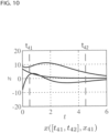
- Figure 10 shows the time-series data in the time interval: t 41 t 42
- Figure 11 shows the time-series data in the time interval: t 51 t 52
- Figure 12 shows the time-series data in the time interval: t 61 t 62
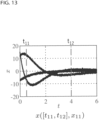
- Figures 13 through 18 show the time-series data including noise. Specifically, Figure 13 shows the time-series data in the time interval: t 11 t 12
- Figure 14 shows the time-series data in the time interval: t 21 t 22
- Figure 15 shows the time-series data in the time interval: t 31 t 32
- Figure 16 shows the time-series data in the time interval: t 41 t 42
- Figure 17 shows the time-series data in the time interval: t 51 t 52
- Figure 18 shows the time-series data in the time interval: t 61 t 62
- the signals in Figs. 13 to 18 are the signals in Figs. 7 to 12 plus noise with mean 0 and variance 0.1, respectively.
- G ⁇ has the following pattern of sign. + 0 ⁇ 0 + ⁇ ⁇ ⁇ +
- * indicates that the sign is unknown.
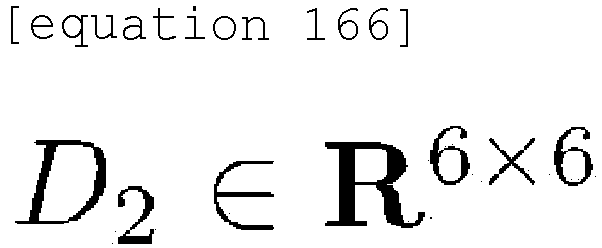
- D 2 ⁇ R 6 ⁇ 6 and d 2 ⁇ R 6 are related to (21) and used in (23).
- ⁇ ⁇ R 6 corresponds to: rvec X of (21).
- one of the goals was to estimate the "ease of control" index when the input channel to each node of the network is fixed (Problem 1(i)).
- Problem 3 is to estimate the value of the controllability Gramian from the data when the A matrix is varied by ⁇ for the system in Equation (1). This problem appears, for example, when applying state feedback to the system or when adjusting the connection strength between nodes in a network system.
- ⁇ ⁇ ⁇ R n ⁇ n is a matrix such that: A ⁇ + ⁇ ⁇ is stable, and: Q ⁇ S n is a symmetric matrix.
- equation (36) has a unique solution.
- Equation (40) can be rewritten as: [equation 203]
- D ⁇ 1 rvec Y D ⁇ 2 rvec Q equivalently.
Landscapes
- Engineering & Computer Science (AREA)
- Physics & Mathematics (AREA)
- General Physics & Mathematics (AREA)
- Mathematical Physics (AREA)
- Theoretical Computer Science (AREA)
- Data Mining & Analysis (AREA)
- Pure & Applied Mathematics (AREA)
- Mathematical Optimization (AREA)
- Mathematical Analysis (AREA)
- Computational Mathematics (AREA)
- Software Systems (AREA)
- Algebra (AREA)
- Databases & Information Systems (AREA)
- General Engineering & Computer Science (AREA)
- Computing Systems (AREA)
- Automation & Control Theory (AREA)
- Medical Informatics (AREA)
- Evolutionary Computation (AREA)
- Health & Medical Sciences (AREA)
- Computer Vision & Pattern Recognition (AREA)
- Artificial Intelligence (AREA)
- Feedback Control In General (AREA)
Abstract





a data acquisition unit that acquires a set of time-series state data:

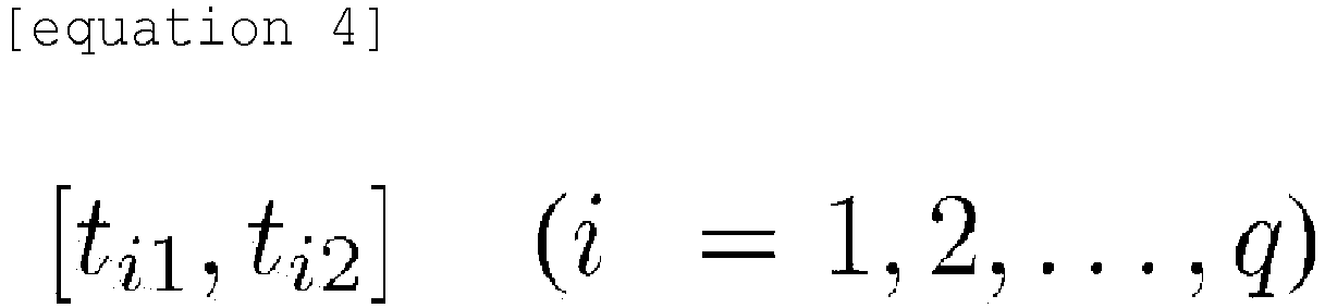
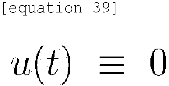
a controllability Gramian calculation unit that defines:

[equation 74]

[equation 81]






an output unit that outputs the input matrix when the controllability Gramian is maximized based on the estimated maximization condition.
Description
- This disclosure relates to a data processing device, a control system, a data processing method and a program.
- A controllability Gramian is known as an indicator for controllability of a system, see, for example, Non-Patent Document 1-6. Whether a system is controllable can be determined by whether the controllability Gramian is regular. Furthermore, the magnitude of the eigenvalues of the controllability Gramian quantitatively indicates the degree of influence of the input on the state.
-
- Non-Patent Literature 1 : F. Pasqualetti, S. Zampieri, and F. Bullo, "Controllability metrics, limitations and algorithms for complex networks," IEEE Transactions on Control of Network Systems, vol. 1, no. 1, pp. 40-52, 2014.
- Non-Patent 2 : V. Tzoumas, M.A. Rahimian, G.J. Pappas, and A. Jadbabaie, "Minimal actuator placement with bounds on control effort," IEEE Transactions on Control of Network Systems, vol. 3, no. 1, pp. 40-52, 2016.
- Non-patent 3 : K. Kashima, "Noise response data reveal novel controllability Gramian for nonlinear network dynamics," Scientific Reports vol. 6, Art. 27300, 2016.
- Non-Patent 4 : V.M. Preciado and M.A. Rahimian, "Controllability Gramian spectra of random networks," 2016 American Control Conference, pp. 3874-3879, 2016.
- Non-Patent 5 : X. Cheng and J.M.A. Scherpen, "A new controllability Gramian for semistable systems and its application to approximation of directed networks," 56th Annual Conference on Decision and Control, pp. 3823-3828, 2017.
- Non-Patent 6 : S. Zhao and F. Pasqualetti, "Networks with diagonal controllability Gramians: analysis, graphical conditions, and design algorithms," Automatica, vol. 102, pp. 10-18, 2019.
- Non-Patent 7 : Z. Wang and D. Liu, "Data-based controllability and observability analysis of linear discrete-time systems," IEEE Transactions on Neural Networks, vol. 22, no. 12, pp. 2388-2392, 2011.
- Non-Patent 8 : D. Bhattacharjee, B. Klose, G.B. Jacobs, and M.S. Hemati, "Data-driven selection of actuators for optimal control of airfoil separation," Theoretical and Computational Fluid Dynamics, vol. 34, no. 4, pp. 557-575, 2020.
- Non-Patent Document 9 : K. Zhou, J.C. Doyle, and K. Glover, Robust and Optimal Control, Prentice Hall, 1996.
- Non-Patent Document 10 : C. Kenney and G. Hewer, "Trace norm bounds for stable Lyapunov operators," Linear Algebra and its Applications, vol. 221, pp. 1-18, 1995.
- A Controllability Gramian can be easily calculated if a mathematical model of a system is known. Hereinafter, calculation methods based on the mathematical model of a system are called "model-based methods". However, the amount of data necessary for modeling the system is not always available. In such cases, a mathematical model of the system cannot be obtained.
- In contrast to the model-based method, calculation methods that calculate based on data of a state trajectory of a system without using a mathematical model are called "data-driven methods". Data-driven methods have the advantage of requiring fewer decision variables than model-based methods because they do not need to identify a mathematical model of the system.
- Methods for estimating controllability Gramians, see, for example, Non-Patent Document 7, and maximizing controllability Gramians, see, for example,
Non-Patent Document 8, using data-driven methods are known. Both of these methods are discrete-time models formulated on the basis of discrete time. However, the physical information contained in the data is represented clearly in the continuous-time model, which is formulated on the basis of continuous time, whereas the discrete-time model has a problem of unclarity. In other words, conventional discrete-time models have the problem that it is difficult to utilize prior knowledge about the characteristics of continuous-time systems. - The purpose of this disclosure is to estimate the controllability Gramian for a system of which mathematical model is unknown, using a data-driven method for continuous-time systems.
- In order to solve the above problem, a data processing device according to an embodiment of this disclosure estimates the limit:


- This data processing device comprises:
- a data acquisition unit that acquires a set of time-series state data:


- a controllability Gramian calculation unit that defines:

[equation 74]

data acquisition unit 10, calculates:
[equation 81]


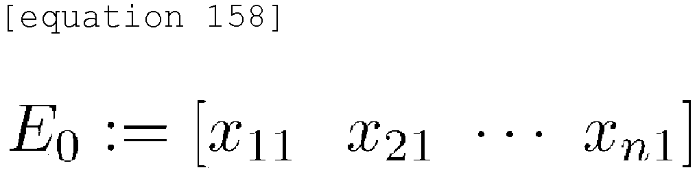
- an output unit that outputs the controllability Gramian estimated by the controllability Gramian calculation unit.
- In one embodiment, the set of time-series state data acquired by the data acquisition unit may include noise and the controllability Gramian calculation unit estimates:
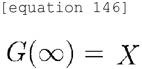
[equation 108]

- In one embodiment, the controllability Gramian calculation unit performs numerical calculations using prior knowledge about the signs of some or all of the matrix components of the solution X.
- Another embodiment of this disclosure is also a data processing device. This data processing device estimates the matrix B which maximizes the trace:


- This data processing device comprises:
- a data acquisition unit that acquires a set of time-series state data:


- a maximization condition calculation unit that estimates the matrix B which maximizes:



- an output unit that outputs the input matrix when the controllability Gramian is maximized based on the estimated maximization condition.
- In one embodiment, the maximization condition calculation unit may obtain a first input matrix:


- In one embodiment, the maximization condition calculation unit may obtain a second input matrix:


- Yet another embodiment of this disclosure is a control system. This control system controls external control objects. This control system comprises:
- a sensor that detects a set of time-series state data from the control objects;
- the aforementioned data processing device; and
- a control unit to control the control objects,
- wherein the sensor transmits the detected set of state data to the data acquisition unit of the data processing device,
- wherein the data processing device transmits the estimated:

- wherein the control unit controls the control objects based on:

- Yet another embodiment of this disclosure is a data processing method. This method estimates the limit:


- This method comprises:
- acquiring a set of time-series state data:


- defining:

[equation 74]

data acquisition unit 10, calculating:
[equation 81]


- outputting the estimated controllability Gramian.
- Yet another embodiment of this disclosure is also a data processing method. This method estimates the matrix B which maximizes the trace:


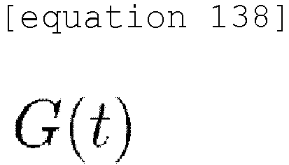


This method comprises: - acquiring a set of time-series state data:


- estimating the matrix B which maximizes:


; and - outputting the input matrix when the controllability Gramian is maximized based on the estimated maximization condition.
- Another embodiment of this disclosure is a program. This program estimates the limit:
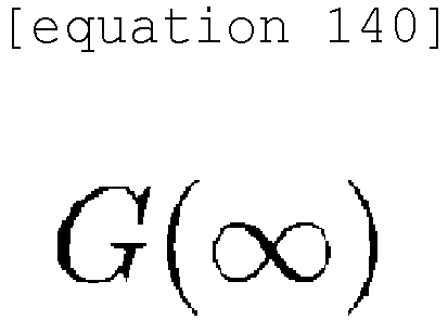


- This program causes the computer to perform the method, comprising:
- acquiring a set of time-series state data:

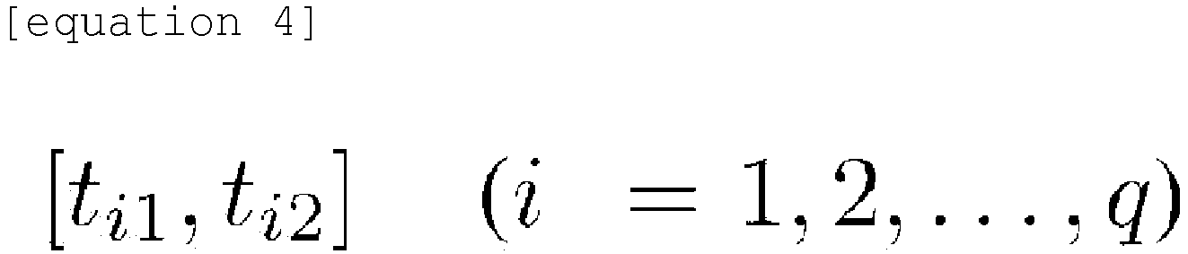
- for the following q time intervals:

- when:

- holds;
- defining:

- expressed as:
[equation 74]
- based on the sets of state data:

- acquired by the
data acquisition unit 10, calculating:
[equation 81]

- and estimating:

- by numerically obtaining the solution X of the following linear equation:

- with respect to:


- outputting the estimated controllability Gramian.
- Yet another embodiment of this disclosure is also a program. This program estimates the matrix B which maximizes the trace:


- This program causes the computer to perform the method, comprising:
- acquiring a set of time-series state data:


- estimating the matrix B which maximizes:


; and - outputting the input matrix when the controllability Gramian is maximized based on the estimated maximization condition.
- Yet another embodiment of this disclosure is a data processing device. This data processing device estimates:


- a data acquisition unit that acquires a set of time-series state data:


- a controllability Gramian calculation unit that defines:

[equation 74]

data acquisition unit 10, calculates:
[equation 81]


[equation 225]


an output unit that outputs the estimated controllability Gramian. - Any combination of the above components, and any transformation of the expression of the invention among devices, methods, systems, recording media, computer programs, etc., is also valid as a form of the invention.
- According to the present disclosure,
the controllability Gramian for a system of which mathematical model is unknown can be estimated, using a data-driven method for continuous-time systems. -
-
Fig. 1 is a functional block diagram of a data processing system according to the first embodiment; -
Fig. 2 is a functional block diagram of a data processing system according to the second embodiment; -
Fig. 3 is a functional block diagram of a control system according to the seventh embodiment; -
Fig. 4 is a functional block diagram of a control system according to the eighth embodiment; -
Fig. 5 is a flowchart showing the processing procedure of a data processing method according to the ninth embodiment; -
Fig. 6 is a flowchart showing the processing procedure of a data processing method according to the tenth embodiment; -
Fig. 7 shows time series data without noise in the time interval:
-
Fig. 8 shows time series data without noise in the time interval:
-
Fig. 9 shows time series data without noise in the time interval:
-
Fig. 10 shows time series data without noise in the time interval:
-
Fig. 11 shows time series data without noise in the time interval:
-
Fig. 12 shows time series data without noise in the time interval:
-
Fig. 13 shows time series data with noise in the time interval:
-
Fig. 14 shows time series data with noise in the time interval:
-
Fig. 15 shows time series data with noise in the time interval:
-
Fig. 16 shows time series data with noise in the time interval:
-
Fig. 17 shows time series data with noise in the time interval:
-
Fig. 18 shows time series data with noise in the time interval:
and -
Fig. 19 is a functional block diagram of a control system for a variant according to the seventh embodiment. - The disclosure will be explained below with reference to drawings based on suitable embodiments. The embodiments are examples rather than limitations of the disclosure. All features or combinations of features described in the embodiments are not necessarily essential to the disclosure. Identical or equivalent components, parts, and processes shown in each drawing shall be given the same symbol, and redundant explanations will be omitted where appropriate. The scale and shape of each part shown in each drawing are set for convenience in order to facilitate explanation, and are not to be construed as limiting unless otherwise noted. When terms such as "first," "second," etc. are used in this specification or in the claims, unless otherwise mentioned, these terms do not indicate any order or degree of importance, but are intended only to distinguish one configuration from another. In addition, in each drawing, some parts of the components that are not important in explaining the embodiments are omitted.
- Before describing the specific embodiments, let us first explain the basic findings.
- The following are definitions of mathematical symbols used herein.
- R: real number.
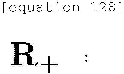

- non-negative real number.

- n × n symmetric matrix.

- n × n diagonal matrix.
- 0: zero matrix.
- I: unit matrix.

- the i-th standard basis of the n-dimensional real vector space.
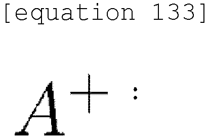
- Moore-Penrose pseudo-inverse of matrix A.

- : the maximum eigenvalue of real symmetric matrix of which all eigenvalues are real numbers.

- trace of square matrix A.
- Note that for any square matrices A and B:


- Furthermore, for an n × n symmetric matrix P of which (i, j) components are:


- For example,:


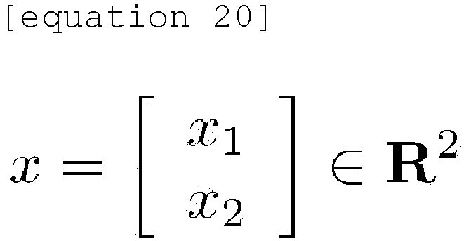

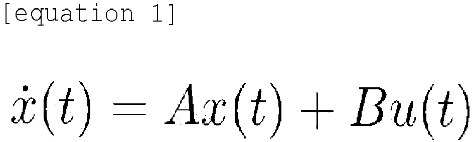
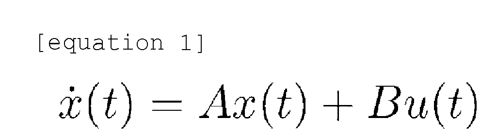
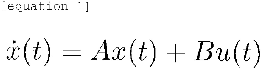
- [Linear Systems and controllability Gramians] We consider the following linear system.
[equation 24]
- Here,:


- In this case, the controllability Gramian:

[equation 29]
- Here,:

- The controllability Gramian represents the set of states that can be reached at time t, starting from the initial state given a control input:


- The set of states that can be reached in this case is expressed as below.

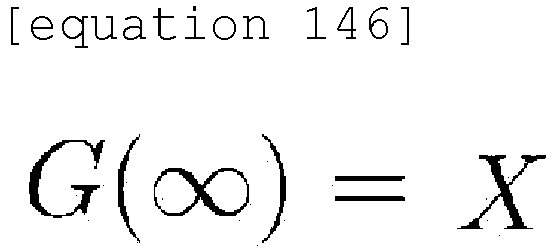
- In particular, the direction that can be reached can be quantified by the limit of controllability Gramians:

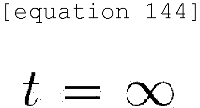


- Therefore,:

- The following lemma is the basis for the computation of the controllability Gramian, see, for example, Non-Patent Literature 9.
- For the system shown in (1), we consider the Lyapunov equation as below.
[equation 34]
- Here,:


- [Data-driven estimation and maximization problem] Once the mathematical model of (1) is obtained, the controllability Gramian:

- We denote the state (1):


- Also, we denote the segment of the state trajectory in the time interval under the same boundary conditions and inputs as above:


- Therefore, the problem of estimating and maximizing:

- For the system shown in (1), let matrix A be a Hurwitz matrix and unknown. Let a set of data:

- Here,:

- (i) We estimate:

- (ii) We obtain the input matrix:


- Here,:

- Note the following four points. First, in Problem 1(i), the input matrix B is assumed to be known. On the other hand, the main objective of Problem 1(ii) is to find the optimal input channel for controlling the system. From this point of view, Problem 1(i) corresponds to a performance analysis of the input matrix B. Namely, in this case,
the input matrix B is evaluated to measure the performance of the following.
- Second, in general,:


- Third, although B can be chosen flexibly, the following two settings are essential.


- The former is the case where the inputs to the system are completely arbitrary. The latter is useful when the system is a network of n nodes, with one input added to each node. As for the other settings of B, approximate solutions can be obtained from the above settings. This may be obtained, for example, by truncating less influential part of B, as in the low-rank matrix approximation based on singular value decomposition.
- Fourth, it is assumed that the resulting set of data is a continuous-time signal and contains no noise. However, even if this assumption does not hold, the method described herein is still applicable to the above problem. This point is discussed below.
- We consider the system (1) with B = 0.
[equation 50]
- In this system, the Lyapunov equation is given by the following.
[equation 51]
- Here,:


- We now consider solving (5) when A is unknown and a set of state trajectory data is given. The problem is formulated as follows.
- We assume that the matrix A is a Hurwitz matrix and is unknown with respect to the system shown in (4). We assume that a symmetric matrix:




- The solution to
Problem 2 is given as follows. We consider the state trajectory x in (4) from the initial state x(0) .
[equation 56]
[equation 57]

- The left side of (7) is equal to:

[equation 59]
[equation 60]
- The following q equations are obtained by applying the sets of data in
Problem 2 to (9).
[equation 61]
- Here, (10) can be considered to be a linear equation for an unknown matrix Y because:

[equation 63]
- Here,:


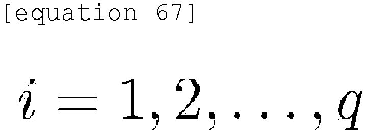
- The solution to
Problem 2 is thus obtained as follows. - We consider
Problem 2. If:
[equation 68]
-
Lemma 2 shows that the solution toProblem 2 can be obtained by solving the linear equation (10), namely (11), using a set of state orbit data for the system shown in (4). - The solution of Problem 1(i) is described below.
- According to the
aforementioned Lemma 1, Problem 1(i) comes down to solving the Lyapunov equation (3) by a data-driven method. Below, we obtain the solution of (3) based on data using the same method that yielded (10). Similar to (6), we make the quadratic form of the state x(t) when B = 0 on the left side of (3) and (1).
- However, in this case, unlike in (8), we cannot replace:


- Therefore first, we introduce the following system defined by the transpose matrix of matrix A:
[equation 74]


- Here, we make the quadratic form:

[equation 79]
- On the other hand,:
[equation 80]
- Therefore, we obtain:
[equation 81]
- However, in this case, the set of data for the state trajectory in (13) in
Problem 1 is not obtained. This difficulty can be resolved by the following result. - We consider:

Problem 1. We assume:

- It can be considered that the chosen data are:

[equation 84]

- If:


- Here,:

- We consider data points:


- The product of:


- By obtaining this relation for j = 1, 2, ..., n, the following is obtained for t.


- This means that:


- We can transform the set of data in
Problem 1 into the set of data in the state trajectory in (13) by this lemma. Note that the assumption of:
- The linear equation:
[equation 84]

- This is expressed as:
[equation 102]


- As a result, the solution to
Problem 1 is obtained as follows. - We consider Problem 1(i). We assume the following.

- If:
[equation 103]
- According to
Theorem 1, the solution of Problem 1(i) is given as the solution of the linear equation (20). - In the above discussion, it was assumed that the set of data obtained is a continuous-time signal and contains no noise. However, this is not limited to this, and as shown below, the aforementioned results can also be applied to data containing noise.
- We assume that data:

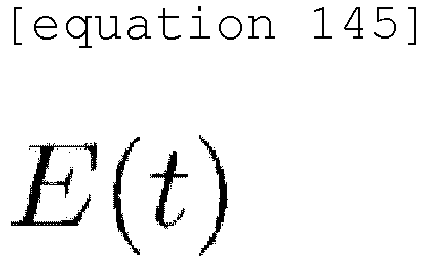

Lemma 3. Therefore,:


- . Then, from (19) and the properties of the Moore-Penrose pseudo-inverse, the relationship:

[equation 108]
- Here,:


- Next, we assume that the sets of data are given as acyclic sample data of state orbitals. The left side of (20) consists of the endpoints of each state trajectory and can be computed from the sample data of the state trajectories. In contrast, the right side of (20) is the integral of the quadratic form of the state orbit. This can be computed approximately from sample data, for example, using the trapezoidal formula. By applying these principles, an approximate solution to the above problem can be obtained.
- The solution of Problem 1(ii) is described below.
- The following shows the maximization of the controllability Gramian:

- For the system shown in (1), we assume that matrix A is a Hurwitz matrix. We consider the following maximization problem:
[equation 110]

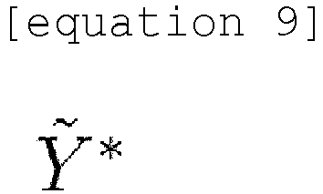
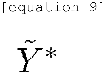
- We define Y* as follows.
[equation 111]
- (i) We define the unit eigenvector:


[equation 115]
- (ii) We assume that:
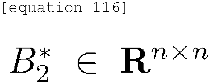


[equation 119]


-
- (i) See, e.g.,
Non-Patent Document 10. - (ii) We define the i-th diagonal component of matrix B as the following.

[equation 122]


[equation 126]


- . On the other hand, from the definitions of (29) and:


- . Further,:

-
Lemma 4 means that, the input matrix that maximizes:


- Therefore, from
Lemma 2 andLemma 4, the following holds. - We consider Problem 1(ii). We assume that (12) hold with respect to the set of data given in
Problem 1. We assume that:
[equation 61]

- Furthermore, in
Lemma 4, we assume that:

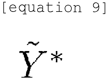


- In this case, the following proposition holds.
- (i) The input matrix:


- (ii) The input matrix:


-
Theorem 2 shows that the solution of Problem 1(ii) can be obtained by solving the linear equation (10) and forming the input matrix by the method ofLemma 4. -
Figure 1 is a functional block diagram of adata processing device 1 according to the first embodiment. Thedata processing device 1 comprises adata acquisition unit 10, a controllabilityGramian calculation unit 12 and anoutput unit 15. Thedata processing device 1 estimates the limit:


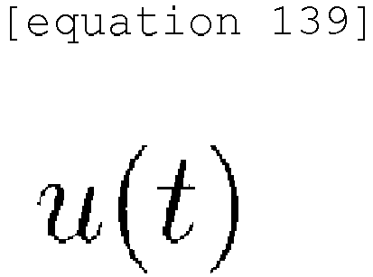
- The
data acquisition unit 10 acquires a set of time-series state data in a plurality of time intervals. In the following description, thedata acquisition unit 10 acquires a set of time-series state data:

- The controllability
Gramian calculation unit 12 defines:
[equation 74]

data acquisition unit 10, calculates:
[equation 81]


- The
output unit 15 outputs the controllability Gramian estimated by the controllabilityGramian calculation unit 12. - Here, the control objects are, for example, the following.
- (Example 1) Power system. The time series data include the amount of electricity generated, the amount of electricity used, temperature and humidity, etc. at each power plant.
- (Example 2) Robots. Time-series data include load, posture, external force and motion state, etc.
- (Example 3) Human body. Time-series data include blood pressure, pulse rate, body temperature and blood composition, etc.
- (Example 4) Chemical plant. Time-series data include temperature, humidity, atmospheric pressure and amount of dust in the air, etc.
- (Example 5) Equipment to be maintained. Time-series data include failure alarm frequency, electrical resistance, metal fatigue and heat generation, etc.
- These control objects are configured as network systems. The mathematical model describing the time-series data output from these systems are complex, and generally such a mathematical model itself is unknown. In contrast, by estimating and outputting controllability Gramians using this implementation, it is possible to determine which node of the control objects configured as network systems should be controlled as the input channel, while the mathematical model is still unknown. The above features are also common to all of the following forms.
- According to this embodiment, the controllability Gramian can be estimated using a data-driven method based on a set of acquired continuous-driven state data for a system of which mathematical model is unknown.
- The set of time-series state data acquired by the data acquisition unit may include noise. In this case, the controllability
Gramian calculation unit 12 estimates:
[equation 108]


- According to this embodiment, controllability Gramians can be estimated using a data-driven method even when the state data contains noise.
- When the state data contains noise, knowledge about the signs of some or all of the matrix components of the solution X of (23) may be given as prior knowledge. In this case, the controllability
Gramian calculation unit 12 performs numerical calculations using such prior knowledge. - According to this method, controllability Gramians can be estimated more accurately using a data-driven method, even when the state data contains noise.
-
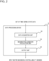
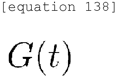
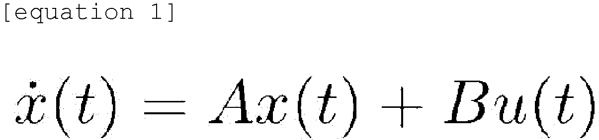
Figure 2 shows a functional block diagram of adata processing device 1 according to the fourth embodiment. Thedata processing device 2 comprises adata acquisition unit 10, a maximizationcondition calculation unit 14, and anoutput unit 15. Thedata processing device 2 estimates the matrix B which maximizes the trace:





- The
data acquisition unit 10 acquires sets of time-series state data in a plurality of time intervals. In the following description, thedata acquisition unit 10 acquires a set of time-series state data:

- The maximization
condition calculation unit 14 estimates the matrix B which maximizes:


data acquisition unit 10. - The
output unit 15 outputs the input matrix when the controllability Gramian is maximized based on the maximization condition estimated by the maximizationcondition calculation unit 14. - According to this embodiment, for a system of which mathematical model is unknown, the input matrix when the controllability Gramian is maximized can be estimated using a data-driven method based on a set of acquired continuous-time state data.
- In the fifth embodiment, the maximization
condition calculation unit 14 obtains a first input matrix:


- According to this embodiment, effective input matrix can be obtained when:

- In the sixth embodiment, the maximization condition calculation unit obtains a second input matrix:


- According to this embodiment, effective input matrix can be obtained when:

-
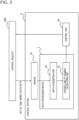
Figure 3 shows a functional block diagram of thecontrol system 3 according to the seventh embodiment. Thecontrol system 3 comprises asensor 16, adata processing device 1 and acontrol unit 18. Thedata processing device 1 comprises adata acquisition unit 10 and a controllabilityGramian calculation unit 12. Namely, thedata processing device 1 is configured and operates the same as thedata processing device 1 inFigure 1 . Thecontrol system 3 controls external control objects 100 by inputting control signals to the control objects 100. - The
sensor 16 detects a set of time-series state data from the control objects 100. Thesensor 16 then transmits the detected set of state data to thedata acquisition unit 10 of thedata processing device 1. Thedata processing device 1 estimates:
control unit 18. Thecontrol unit 18 generates control signals based on:
- According to this embodiment, it is possible to detect time-series state data from an external control object, to estimate the controllability Gramian using a data-driven method based on the detected set of state data and appropriately to control said control object based on the estimated controllability Gramian.
-
Figure 19 is a functional block diagram of thecontrol system 5 according to a variant of the seventh embodiment.Control system 5 comprises asensor 16,data processing device 1 and acontrol unit 19. Thedata processing device 1 comprises adata acquisition unit 10 and a controllabilityGramian calculation unit 12. Thecontrol unit 19 has a control inputvalue determination unit 191 and an inputchannel determination unit 192. Namely, thecontrol system 5 differs from thecontrol system 3 inFigure 3 in that thecontrol unit 19 includes the control inputvalue determination unit 191 and the inputchannel determination unit 192. Other configurations of thecontrol system 5 are common to thecontrol system 3. In the following, we will focus on the parts that differ from thecontrol system 3 and omit redundant explanations. - The control input
value determination unit 191 is sent the set of state data detected by thesensor 16. Based on this set of state data, the control inputvalue determination unit 191 determines what control should be performed on the control object determined by the inputchannel determination unit 192. The control inputvalue determination unit 191 sends the determined control contents to the inputchannel determination unit 192. - The input
channel determination unit 192 is sent the estimated controllability Gramian. The inputchannel determination unit 192 determines which of the control objects 100 should be controlled based on this controllability Gramian. The inputchannel determination unit 192 selects the determined control object and executes the control determined by the control inputvalue determination unit 191 on the selected control object. - According to this embodiment, it is possible to detect time-series state data from external control objects, to estimate controllability Gramians using a data-driven method based on a set of detected state data, to select an appropriate control object based on the estimated controllability Gramians and appropriately to control the selected control object.
-
Figure 4 is a functional block diagram of thecontrol system 4 according to the eighth embodiment. Thecontrol system 4 comprises asensor 16, adata processing device 2 and acontrol unit 18. Thedata processing device 2 comprises adata acquisition unit 10 and a maximizationcondition calculation unit 14. Namely, thedata processing device 2 is configured the same as thedata processing unit 2 inFigure 2 and operates the same. Thecontrol system 4 controls external control objects 100 by inputting control signals to thecontrol object 100. - The
sensor 16 detects a set of time-series state data from the control objects 100. Thesensor 16 transmits the detected set of state data to thedata acquisition unit 10 of thedata processing device 1. Thedata processing device 2 estimates the matrix B which maximizes:
control unit 18. Thecontrol unit 18 generates control signals based on the matrix B and uses them to control the control objects 100. - According to this embodiment, it is possible to detect time-series state data from external control objects, to estimate the input matrix when the controllability Gramian is maximum using a data-driven method based on the detected set of state data, and appropriately to control the control objects based on the estimated input matrix.
-
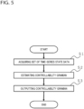
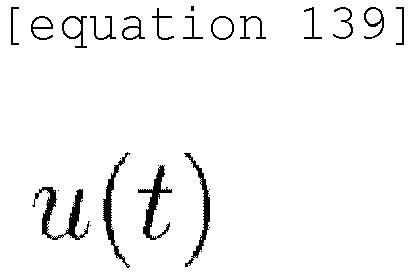
Figure 5 is a flowchart showing the processing procedure of the data processing method according to the ninth embodiment. This method estimates the limit:


- In step S1, the method obtains the time-series state data set:


- In step S2, the method defines:

[equation 74]
[equation 81]


- In step S3, the method outputs the controllability Gramian estimated in step S2.
- According to this embodiment, the controllability Gramian can be estimated by a computer using a data-driven method based on a set of acquired continuous-time state data for a system of which mathematical model is unknown.
-
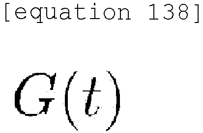
Figure 6 is a flowchart showing the processing procedure of the data processing method according to the tenth embodiment. - This method estimates the matrix B which maximizes the trace:






- In step S1, the method obtains the time-series state data set:


- In step S4, the method estimates the matrix B which maximizes:


- In step S5, the method outputs the input matrix when the controllability Gramian is maximized based on the maximization condition estimated in step S4.
- According to this embodiment, the input matrix when the controllability Gramian is maximized can be estimated by a computer using a data-driven method based on a set of acquired continuous-time state data for a system of which mathematical model is unknown.
- The eleventh embodiment is a program. This program estimates the limit:


- This program make a computer perform the step of obtaining the time-series state data set:


the step of defining:
[equation 74]
[equation 81]



the step of outputting the estimated controllability Gramian. - According to this embodiment, software can be implemented as a program to estimate the controllability Gramian using a data-driven method based on a set of acquired continuous-time state data for a system of which the mathematical model is unknown.
- The twelfth embodiment is a program. This program estimates the matrix B which maximizes the trace:


- This program make a computer perform
the step of obtaining the time-series state data set:

the step of estimating the matrix B which maximizes:


the step of outputting the input matrix when the controllability Gramian is maximized based on the estimated maximization condition. - According to this embodiment, software can be implemented as a program to estimate the input matrix when the controllability Gramian is maximized by a computer using a data-driven method based on a set of acquired continuoustime state data for a system of which mathematical model is unknown.
- The following shows the results by the first embodiment with respect to a set of noiseless time-series state data are presented. We obtain the solution of Problem 1(i) in the system shown in (1) when:


- For comparison, the true values of controllability Gramians:


-
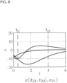
Figures 7 through 12 show the time-series data without noise. Specifically,
Figure 7 shows the time-series data in the time interval:
-
Figure 8 shows the time-series data in the time interval:
-
Figure 9 shows the time-series data in the time interval:
-
Figure 10 shows the time-series data in the time interval:
-
Figure 11 shows the time-series data in the time interval:
-
Figure 12 shows the time-series data in the time interval:
- The
data acquisition unit 10 of thedata processing device 1 inFig. 1 acquires time-series state data sets:
Figs. 7 through 12 . In this case,:


- This means the following.

- Therefore, (22) holds and there exists a unique solution X to the linear equation (22).
- The controllability
Gramian calculation unit 12 solves (22) numerically to obtain the following values.
[equation 162]
- This is consistent with the true value (30), indicating the usefulness of this embodiment.
- The following shows the results by the second embodiment with respect to a set of time-series state data including noise.
Figures 13 through 18 show the time-series data including noise. Specifically,
Figure 13 shows the time-series data in the time interval:
-
Figure 14 shows the time-series data in the time interval:
-
Figure 15 shows the time-series data in the time interval:
-
Figure 16 shows the time-series data in the time interval:
-
Figure 17 shows the time-series data in the time interval:
-
Figure 18 shows the time-series data in the time interval:
Figs. 13 to 18 are the signals inFigs. 7 to 12 plus noise withmean 0 and variance 0.1, respectively. - The controllability
Gramian calculation unit 12 solves (23) numerically to obtain the following values.
[equation 163]
- The following is the actual result obtained using the third embodiment with respect to sets of time-series state data including noise. In this case, the sets of the time-series state data are also shown in
Figs. 13 through 18 , as described above. - Here, we assume that we have prior knowledge that:


[equation 165]
- Here, :


- The following describes the results obtained from the fourth embodiment using the data in
Figures 7 through 12 . In this case,:


- Numerical calculation in the embodiment yields the following.

- The following is the results obtained from the fifth embodiment using the data in
Figures 7 through 12 . The first input matrix:




components 1/3 is used as an example for comparison. - This is clearly smaller than the value:

- The following are the results obtained from the sixth embodiment using the data in
Figures 7 through 12 . The second input matrix:


- The values of:


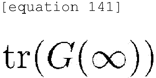
[Table 1] B tr(G(∞)) [ e 1 0 0]1.500 [0 e2 0] 0.500 
6.750 - In the embodiments described above, one of the goals was to estimate the "ease of control" index when the input channel to each node of the network is fixed (Problem 1(i)).
- In other words, the following problems were discussed.
- For the system shown in Equation (1), we assume that the matrix A is a Hurwitz matrix and is unknown. We assume that a set of data:


- (i) :


- In other words, in the embodiments explained above, it was assumed that the amount of action between each node constituting the network, i.e., the strength of the connection between nodes and an indicator of the amount of transmitted data, are all fixed values. In this case, it was possible to know how to select input channels to improve ease of control. In contrast, the following describes the estimation of ease of control when the amount of action is adjusted, i.e., estimation of controllability Gramian when the amount of action changes. The goal is to know how to adjust the action amount in order to improve the ease of control.
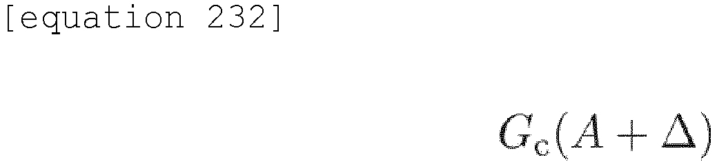
- In the following, we consider the estimation of the controllability Gramian when a change Δ is added to an unknown matrix A. This problem can be formulated as follows.
- We consider the system in Equation (1). Here, we assume that:


[equation 182]
- Here,:


-
Problem 3 is to estimate the value of the controllability Gramian from the data when the A matrix is varied by Δ for the system in Equation (1). This problem appears, for example, when applying state feedback to the system or when adjusting the connection strength between nodes in a network system. - [Data-driven solution of the Lyapunov equation] In the following, we describe a method for solving the Lyapunov equation using the state trajectories of the system as a preparation for
Problem 3. We consider the following system:
[equation 187]
- Here,:


- For this system, we consider the following Lyapunov equation.
[equation 190]
- Here,:


- At this point, we consider the following problem
- We consider the system in Equation (35). Here,:

Problem 3. Also, we assume that:


- The solution to
Problem 4 is given as follows. First, for both sides of equation (36), we consider the quadratic form with respect to the state trajectory:
[equation 196]
[equation 198]

- Furthermore,:
[equation 199]

- Here, N linear equations for the unknown number Y:
[equation 201]

- Next, we consider rewriting equation (40) in a matrix-based form. First, equation (39) can be expressed as:
[equation 202]
[equation 203]


- The solution to
Problem 4 is then obtained as follows. - We consider
Problem 4. If:
[equation 68]
Problem 4. (End of Theorem 3). - Next, we consider the solution to
Problem 3. -

Theorem 3 if state trajectory data of:
[equation 74]
Lemma 1, the controllability:
[equation 208]
- Similarly to the above discussion,:
[equation 212]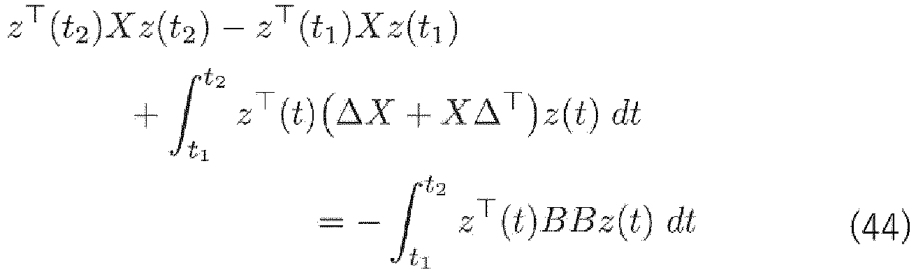


- However, in
Problem 3, the state trajectory of the system in Equation (13) is not generally available except in the case that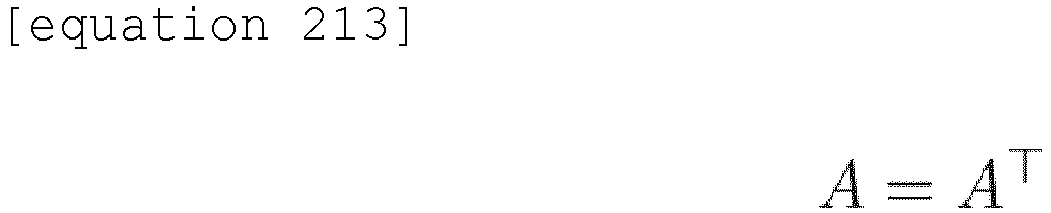
Problem 3. On the other hand, if the state trajectory of the system in Equation (35) can be transformed into the state trajectory of the system in Equation (13), a solution toProblem 3 can be constructed. Such a data transformation is accomplished by the followingLemma 5. - We express the state trajectory of the system of Equation (13) by:


- . We assume that the state trajectory data D in
Problem 3 is arbitrarily given. Here, we assume that N ≥ n. We assume that, for this D,:


[equation 218]
[equation 221]


- We give the solution to
problem 3 using the above results. First, we assume that the function:

- Then N linear equations:
[equation 225]


Problem 3 and their i-th row:


- Thus, the solution to
Problem 3 can be obtained as follows. - We consider
Problem 3. Here, we assume that N ≥ n. If E0 in Equation (45) is regular and:
[equation 68]
Problem 3. - As in the first embodiment,
Figure 1 is used to describe the data processing device according to the thirteenth embodiment. -
Figure 1 is a functional block diagram of thedata processing device 1 according to the thirteenth embodiment. Thedata processing device 1 comprises adata acquisition unit 10, a controllabilityGramian calculation unit 12 and anoutput unit 15. - The
data processing device 1 estimates:


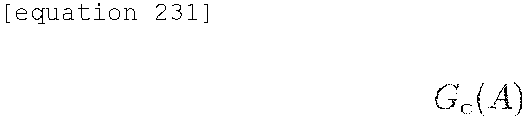


- The
data acquisition unit 10 acquires a set of time-series state data in a plurality of time intervals. In the following description, thedata acquisition unit 10 acquires a set of time-series state data:

- The controllability
Gramian calculation unit 12 defines:
[equation 74]

data acquisition unit 10, calculates:
[equation 81]


[equation 225]
- The
output unit 15 outputs the controllability Gramian estimated by the controllabilityGramian calculation unit 12. - According to this embodiment, the controllability Gramian can be estimated when the amount of action between each node constituting the network changes.
- The present disclosure has been described above based on the embodiments. It is understood by those skilled in the art that these embodiments are examples, that various variations are possible in the combination of each component and each processing process and that such variations are also within the scope of the disclosure.
- Any combination of the above mentioned embodiments and variations is also useful as an embodiment of the disclosure. The new embodiment resulting from the combination will have the respective effects of each of the embodiments and variations that are combined.
- The principle of the disclosure can be applied to the control of systems in various fields as follows. (Application example 1) When the control object is an electric power system, optimal power supply control can be performed based on time-series data of power generation, power consumption, temperature and humidity, etc. at each power plant.
- (Application example 2) When the control object is a robot, optimal posture control can be performed based on time-series data such as load, posture, external force and motion state, etc.
- (Application example 3) When the control object is a human body, optimal medication control can be performed based on time-series data such as blood pressure, pulse rate, body temperature and blood composition, etc.
- (Application example 4) When the control object is a chemical plant, the system can perform optimal operation control based on time-series data such as temperature, humidity, air pressure and the amount of dust in the air, etc.
- (Application example 5) When the control object is equipment maintenance, optimal maintenance control can be performed based on time-series data such as failure alarm frequency, electrical resistance, metal fatigue and heat generation, etc.
-
- 1. Data processing device.
- 2. Data processing device.
- 3. Control system.
- 4. Control system.
- 5. Control system.
- 10. Data acquisition unit.
- 12. Controllability Gramian calculation unit.
- 14. Maximization condition calculation unit.
- 15. Output unit.
- 16. Sensor.
- 18. Control unit.
- 19: Control unit.
- 100: Control object.
- 191: Control input value determination unit.
- 192: Input channel determination unit.
- S1: The step of acquiring a set of time-series state data.
- S2: The step of estimating the controllability Gramian.
- S3: The step of outputting the controllability Gramian.
- S4: The step of estimating the condition when the controllability Gramian is maximum.
- S5: The step of outputting the input matrix when the controllability Gramian is maximized.
Claims (13)
- A data processing device to estimate the limit:


 a data acquisition unit that acquires a set of time-series state data:
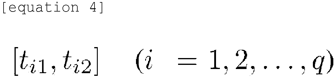
 a controllability Gramian calculation unit that defines:
[equation 74]
[equation 81]


 an output unit that outputs the estimated controllability Gramian.
 - The data processing device according to claim 1,wherein the set of time-series state data acquired by the data acquisition unit includes noise andwherein the controllability Gramian calculation unit estimates:

[equation 108]

- The data processing device according to claim 2,
wherein the controllability Gramian calculation unit performs numerical calculations using prior knowledge about the signs of some or all of the matrix components of the solution X. - A data processing device to estimate the matrix B which maximizes the trace:



 a data acquisition unit that acquires a set of time-series state data:

 a maximization condition calculation unit that estimates the matrix B which maximizes:


; andan output unit that outputs the input matrix when the controllability Gramian is maximized based on the estimated maximization condition. - The data processing device according to claim 4,
wherein the maximization condition calculation unit obtains a first input matrix:

- The data processing device according to claim 4,
wherein the maximization condition calculation unit obtains a second input matrix:


- A control system to control external control objects, comprising:a sensor that detects a set of time-series state data from the control objects;the data processing device according to any one of claims 1 to 3; anda control unit to control the control objects,wherein the sensor transmits the detected set of state data to the data acquisition unit of the data processing device,wherein the data processing device transmits the estimated:
 wherein the control unit controls the control objects based on:
- A control system to control external control objects, comprising:a sensor that detects a set of time-series state data from the control objects;the data processing device according to any one of claims 4 to 6; anda control unit to control the control objects,wherein the sensor transmits the detected set of state data to the data acquisition unit of the data processing device,wherein the data processing device transmits the estimated matrix B which maximizes:
 wherein the control unit controls the control objects based on:.
- A data processing method to estimate the limit:


 acquiring a set of time-series state data:

 defining:
[equation 74]
[equation 81]


 outputting the estimated controllability Gramian.
 - A data processing method to estimate the matrix B which maximizes the trace:


 acquiring a set of time-series state data:

 estimating the matrix B which maximizes:


; andoutputting the input matrix when the controllability Gramian is maximized based on the estimated maximization condition. - A program to estimate the limit:


 wherein the program causes the computer to perform the method, comprising:acquiring a set of time-series state data:

 defining:
[equation 74]
[equation 81]



 outputting the estimated controllability Gramian.
 - A program to estimate the matrix B which maximizes the trace:


wherein the program causes the computer to perform the method, comprising:acquiring a set of time-series state data:

 estimating the matrix B which maximizes:


; andoutputting the input matrix when the controllability Gramian is maximized based on the estimated maximization condition. - A data processing device to estimate:


 a data acquisition unit that acquires a set of time-series state data:

 a controllability Gramian calculation unit that defines:
[equation 74]
[equation 81]


[equation 225]


an output unit that outputs the estimated controllability Gramian.
Applications Claiming Priority (2)
| Application Number | Priority Date | Filing Date | Title |
|---|---|---|---|
| JP2021143668 | 2021-09-03 | ||
| PCT/JP2022/033059 WO2023033132A1 (en) | 2021-09-03 | 2022-09-02 | Data processing device, control system, data processing method, and program |
Publications (2)
| Publication Number | Publication Date |
|---|---|
| EP4398130A1 true EP4398130A1 (en) | 2024-07-10 |
| EP4398130A4 EP4398130A4 (en) | 2025-10-01 |
Family
ID=85412439
Family Applications (1)
| Application Number | Title | Priority Date | Filing Date |
|---|---|---|---|
| EP22864714.5A Pending EP4398130A4 (en) | 2021-09-03 | 2022-09-02 | DATA PROCESSING DEVICE, CONTROL SYSTEM, DATA PROCESSING METHOD AND PROGRAM |
Country Status (6)
| Country | Link |
|---|---|
| US (1) | US20240403384A1 (en) |
| EP (1) | EP4398130A4 (en) |
| JP (1) | JP7688947B2 (en) |
| CN (1) | CN117751360A (en) |
| AU (1) | AU2022339367A1 (en) |
| WO (1) | WO2023033132A1 (en) |
Family Cites Families (6)
| Publication number | Priority date | Publication date | Assignee | Title |
|---|---|---|---|---|
| JPH0499939A (en) * | 1990-08-20 | 1992-03-31 | Mitsubishi Heavy Ind Ltd | Control system design method of electric-hydraulic shaking table |
| WO2003036396A1 (en) * | 2001-10-25 | 2003-05-01 | Aspen Technology, Inc. | Non-linear dynamic predictive device |
| WO2013040076A1 (en) * | 2011-09-12 | 2013-03-21 | Fred Hutchinson Cancer Research Center | Dynamics and control of state-dependent networks for probing genomic organization |
| US20150095000A1 (en) * | 2013-10-02 | 2015-04-02 | Nec Laboratories America, Inc. | Optimal sensor and actuator deployment for system design and control |
| US10142755B2 (en) * | 2016-02-18 | 2018-11-27 | Google Llc | Signal processing methods and systems for rendering audio on virtual loudspeaker arrays |
| RU2714567C1 (en) * | 2019-05-06 | 2020-02-18 | федеральное государственное бюджетное образовательное учреждение высшего образования "Ивановский государственный энергетический университет имени В.И. Ленина" (ИГЭУ) | Automatic adjustment method of regulator |
-
2022
- 2022-09-02 US US18/688,728 patent/US20240403384A1/en active Pending
- 2022-09-02 EP EP22864714.5A patent/EP4398130A4/en active Pending
- 2022-09-02 JP JP2023545687A patent/JP7688947B2/en active Active
- 2022-09-02 AU AU2022339367A patent/AU2022339367A1/en active Pending
- 2022-09-02 CN CN202280053561.0A patent/CN117751360A/en active Pending
- 2022-09-02 WO PCT/JP2022/033059 patent/WO2023033132A1/en not_active Ceased
Also Published As
| Publication number | Publication date |
|---|---|
| JP7688947B2 (en) | 2025-06-05 |
| CN117751360A (en) | 2024-03-22 |
| US20240403384A1 (en) | 2024-12-05 |
| JPWO2023033132A1 (en) | 2023-03-09 |
| WO2023033132A1 (en) | 2023-03-09 |
| EP4398130A4 (en) | 2025-10-01 |
| AU2022339367A1 (en) | 2024-04-04 |
Similar Documents
| Publication | Publication Date | Title |
|---|---|---|
| Sontag | Network reconstruction based on steady-state data | |
| Shi et al. | Machine learning accelerated PDE backstepping observers | |
| Schaeffer et al. | Interpretation of high-dimensional linear regression: Effects of nullspace and regularization demonstrated on battery data | |
| Breschi et al. | Identification of hybrid and linear parameter varying models via recursive piecewise affine regression and discrimination | |
| Elbeyli et al. | A semi-discretization method for delayed stochastic systems | |
| Yusupbekov et al. | Stable algorithms for adaptive control and adaptation of uncertain dynamic objects based on reference models | |
| Castagnotto et al. | Fast H 2-optimal model order reduction exploiting the local nature of Krylov-subspace methods | |
| US20240403384A1 (en) | Data processing equipment, control system, data processing method and program | |
| Zhu et al. | Latent variable regression for process and quality modeling | |
| Lan et al. | Learning a dynamical system model for a spatiotemporal field using a mobile sensing robot | |
| Liu et al. | Slow state estimation for singularly perturbed systems with discrete measurements | |
| US11692857B2 (en) | Distributed process state and input estimation for heterogeneous active/passive sensor networks | |
| Nguyen et al. | Asymptotic inference for hidden process regression models | |
| Farhat et al. | Fault detection for LPV systems: Loop shaping H_ approach | |
| Li et al. | Curriculum-Based Soft Actor-Critic for Multi-Section R2R Tension Control | |
| Bankole et al. | Algorithmic modelling of structural connectivity for process plants | |
| Xiaoqiang et al. | An improved FVS-KPCA method of fault detection on TE process | |
| Pan et al. | Nonparametric infinite horizon Kullback-Leibler stochastic control | |
| Wang et al. | Linear shrinkage for predicting responses in large-scale multivariate linear regression | |
| Mao et al. | System identification with variance minimization via input design | |
| Wang et al. | Model-based predictive control for spatially-distributed systems using dimensional reduction models | |
| Singh et al. | Vector Contraction Analysis for Nonlinear Dynamical Systems | |
| van Belzen et al. | Model reduction of multi-variable distributed systems through empirical projection spaces | |
| Chen et al. | Performance monitoring of MPCA-based control for multivariable batch control processes | |
| Yamada et al. | Study on Efficient Sensor Node Selection for Observability Gramian Optimization⋆ |
Legal Events
| Date | Code | Title | Description |
|---|---|---|---|
| STAA | Information on the status of an ep patent application or granted ep patent |
Free format text: STATUS: THE INTERNATIONAL PUBLICATION HAS BEEN MADE |
|
| PUAI | Public reference made under article 153(3) epc to a published international application that has entered the european phase |
Free format text: ORIGINAL CODE: 0009012 |
|
| STAA | Information on the status of an ep patent application or granted ep patent |
Free format text: STATUS: REQUEST FOR EXAMINATION WAS MADE |
|
| 17P | Request for examination filed |
Effective date: 20240330 |
|
| AK | Designated contracting states |
Kind code of ref document: A1 Designated state(s): AL AT BE BG CH CY CZ DE DK EE ES FI FR GB GR HR HU IE IS IT LI LT LU LV MC MK MT NL NO PL PT RO RS SE SI SK SM TR |
|
| DAV | Request for validation of the european patent (deleted) | ||
| DAX | Request for extension of the european patent (deleted) | ||
| A4 | Supplementary search report drawn up and despatched |
Effective date: 20250903 |
|
| RIC1 | Information provided on ipc code assigned before grant |
Ipc: G06F 17/10 20060101AFI20250828BHEP Ipc: G05B 13/02 20060101ALI20250828BHEP |