EP4383498A1 - Method of forecasting power production/consumption in a distributed network - Google Patents
Method of forecasting power production/consumption in a distributed network Download PDFInfo
- Publication number
- EP4383498A1 EP4383498A1 EP22211594.1A EP22211594A EP4383498A1 EP 4383498 A1 EP4383498 A1 EP 4383498A1 EP 22211594 A EP22211594 A EP 22211594A EP 4383498 A1 EP4383498 A1 EP 4383498A1
- Authority
- EP
- European Patent Office
- Prior art keywords
- nodes
- sequence
- matrices
- time
- interest
- Prior art date
- Legal status (The legal status is an assumption and is not a legal conclusion. Google has not performed a legal analysis and makes no representation as to the accuracy of the status listed.)
- Pending
Links
Images


Classifications
-
- H—ELECTRICITY
- H02—GENERATION; CONVERSION OR DISTRIBUTION OF ELECTRIC POWER
- H02J—ELECTRIC POWER NETWORKS; CIRCUIT ARRANGEMENTS OR SYSTEMS FOR SUPPLYING OR DISTRIBUTING ELECTRIC POWER; SYSTEMS FOR STORING ELECTRIC ENERGY
- H02J3/00—Circuit arrangements for AC mains or AC distribution networks
- H02J3/003—Load forecast, e.g. methods or systems for forecasting future load demand
-
- H—ELECTRICITY
- H02—GENERATION; CONVERSION OR DISTRIBUTION OF ELECTRIC POWER
- H02J—ELECTRIC POWER NETWORKS; CIRCUIT ARRANGEMENTS OR SYSTEMS FOR SUPPLYING OR DISTRIBUTING ELECTRIC POWER; SYSTEMS FOR STORING ELECTRIC ENERGY
- H02J3/00—Circuit arrangements for AC mains or AC distribution networks
- H02J3/004—Generation forecast, e.g. methods or systems for forecasting future energy generation
-
- H—ELECTRICITY
- H02—GENERATION; CONVERSION OR DISTRIBUTION OF ELECTRIC POWER
- H02J—ELECTRIC POWER NETWORKS; CIRCUIT ARRANGEMENTS OR SYSTEMS FOR SUPPLYING OR DISTRIBUTING ELECTRIC POWER; SYSTEMS FOR STORING ELECTRIC ENERGY
- H02J2103/00—Details of circuit arrangements for mains or AC distribution networks
- H02J2103/30—Simulating, planning, modelling, reliability check or computer assisted design [CAD] of electric power networks
Definitions
- the present invention relates to the field of distributed power networks. More particularly, it relates to a method of forecasting power production and/or consumption in a distributed power production and/or consumption network.
- Typical state of the art approaches for renewable energy source production forecasting combine numerical weather predictions, satellite images and ground measurements with physical or machine learning models.
- Such approaches tend to have low spatial and/or temporal resolution of the input data and thus of the resulting forecasts.
- the aim of the present invention is hence to at least partially overcome the above-mentioned drawbacks of the prior art.
- the invention relates to a method of forecasting weather-dependent power resource production and/or consumption, as defined in independent claim 1.
- This method can be carried out on a processing unit such as a general purpose computer and relates to a distributed power system comprising a time-varying plurality N k of first nodes at least some of which comprise of power resources adapted to produce and/or to consume power and which each comprise a sensor S 1 , S 2 , ... S N k adapted to obtain direct or indirect measurements v 1 , v 2 ,..., v N k of insolation and/or temperature at a plurality of timesteps M.
- Direct measurements can, for instance, be obtained from a weather station, whereas indirect measurements can be inferred from consumption of heating, lighting or cooling power of a building.
- the method of the invention comprises steps of:
- This method is robust to changes in the number of first nodes and the corresponding sensors, and does not need to be repeated in its entirety for every such change, or to make forecasts for new points of interest, i.e. for proposed new nodes. This significantly reduces the computing time and power required to carry it out compared to prior art methods.
- said first nodes are grouped into a plurality of clusters in said intermediate network G 1 , said intermediate network G 1 having a predefined number of nodes C, where typically C ⁇ N k .
- said dynamic feature extraction comprises:
- said at least one point of interest is not a node in the output network G 2 . This enables forecasting for a location not in any of the sets of nodes.
- Figure 1 illustrates schematically a distributed power system 1 upon which the method according to the invention can be carried out.
- the distributed power system 1 comprises a plurality of first nodes 3 (of which only a few have been indicated with a reference sign), at least some of which are linked with each other by a power distribution grid as is generally known.
- At least some of said first nodes 3 comprise a power resource arranged to produce and/or consume power, for instance photovoltaic arrays or wind turbines for producing power, and residential, commercial or industrial buildings which consume power.
- Each first node 3 may have one or more power producing and/or power consuming entity associated with a sensor arranged to detect power generated or consumed.
- first nodes 3 may additionally comprise, or may simply be, a weather station comprising a sensor adapted to measure solar irradiance and/or ambient temperature and/or wind speed.
- each of said first nodes 3 comprise or are associated with sensors S 1 , S 2 , ..., S N k arranged to measure quantities which vary according to the weather, whether directly in the case of a weather station or indirectly in the case of power generation or consumption.
- the power generation or consumption observations provide indirect information on the underlying weather phenomena, with sufficient correlation to be exploitable in the present method.
- the sensors S 1 , S 2 , ..., S N k can be considered as forming an input network.
- the first nodes 3 can be divided into clusters 5 and local subgroups as indicated by dividing lines 7, and the location of each sensor is known in terms of at least its latitude and longitude. Its altitude can also be known.
- the number of first nodes 3 is not fixed, and can vary as power resources or weather stations are added to or removed from the power distribution network 1, and this point is key to the invention: the method as described below is robust to such changes, and does not need to be repeated in its entirety for every change in the network 1 or to make forecasts for proposed new nodes 3.
- the model can be updated to take into account new input data without any significant changes to the model architecture and without the need to retrain the models every time a new node 3 needs to be taken into consideration.
- a processing unit which may for instance be a general-purpose computer, distributed cloud computing or similar, carries out the method described below.
- the method of the invention uses graphs to model the spatio-temporal relations of the different signals in the system, that is to say weather station data, power generation or consumption data from various first nodes 3.
- a "graph” in this context is a mathematical model that is composed of a set of nodes 3 (or vertices) and a set of edges that describe the relationship between nodes 3.
- each first node 3 represents a sensor, e.g. a power producing and/or consuming resource providing sensing data about power produced or consumed, or a weather station.
- the edges may represent the spatial proximity between stations or a learned relationship between them.
- the number of first nodes N k in the network may vary at each discrete time k due to a disconnection of some power generation or consumption for example.
- G k denote the graph that models the sensor network at time k .
- the method of the invention outputs forecasts of the desired signals (e.g. power generation or irradiance) for H time steps ahead, i.e.
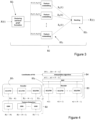
- the forecasting method is depicted in Figure 2 and it comprises four main blocks: the matrix formation block B1, the feature extraction block B2, the forecast block B3 and the interpolation block B4.
- F is the number of measured variables that the sensor network takes, e.g. irradiance, power, temperature, etc.
- the i -th row of the matrix contains the measurements taken at time k by node i . If a first node 3 only measures a subset of the said variables, then a NaN (not a number) symbol is placed in the corresponding columns of the missing measurements.
- the number of measured variables F is fixed for all time steps.
- the second block B2 is a graph feature extraction module that clusters the input nodes in G k into a fixed intermediate network G 1 with a predefined number of second nodes C, typically C ⁇ N k .
- the second nodes C are a subset of the first nodes 3.
- "Features" are characteristics of the data which provide useful information; in other words they are numerical values computed from the raw data which provide salient information about the data.
- the feature extraction method can be chosen from known methods such as the Fourier transform of the raw signals, in which case the extracted features are frequency content of the signals, principal component analysis, in which case the features are the linear transformation of the raw data by the matrix of principal components, or, simply, the output of a neural network that is trained to learn the most salient information for a specific task.
- the local embeddings take into account the local topology, thus, they learn a low dimensional representation of the graph signals such that when nodes are removed or added the model can easily adapt to the new situation.
- This output network G 2 may be different from the intermediate network G 1 with a denser network with more nodes in the region of interest (for instance where it may be desired to place a new node such as a new PV array), i.e. N ⁇ C.
- the forecast module produces forecasts of the desired signals for H time steps ahead in time, i.e.
- the forecast block can use any fixed graph forecast model, e.g. a linear autoregressive model, a graph convolutional transformer or a graph convolutional recurrent neural network to carry out the forecast. Indeed, any multidimensional time-series forecasting can be used.
- the interpolation module forecasts the desired signals in the POI.
- the interpolation block uses graph-based methods that take into account the local and global topology of the input and output networks to produce the final forecasts on the desired nodes.
- Figure 3 illustrates a particular implementation example of the second block B2.
- the third sub-block B2 3 stacks all vectors x ⁇ i (k) into the fixed size matrix X ( k ).
- Figure 4 illustrates an implementation example of blocks B2, B3 and B4 of the method according to the invention.
- Second block B2 uses a generic graph neural network (GNN) to implement the clustering and feature embedding as described above in the context of figure 3 .
- GNN generic graph neural network
- the feature extraction block B2 uses generic GNNs as the functions to implement the clustering B2 1 and feature aggregation B2 2 steps.
- the C clusters and their centroids fixed nodes in G 1
- the local adjacency matrices A i (k) can be constructed using the k nearest neighbours algorithm of using a fully connected graph based on a function ofthe distance between nodes.
- Possible candidates for the feature aggregation function f ( ⁇ ) are:
- learnable parameters in all of the aforementioned functions are independent of N ik , i.e. are independent of the number of nodes at every cluster i and every time step k , thus independent of the number of input sensors at every time step.
- the forecasting module of block B3 is composed of an encoder-decoder model to forecast the desired variables (power or irradiance) at the N fixed locations defined in G 2 .
- Both the encoder B3 1 and decoder B3 2 combine recurrent neural networks and spectral graph convolution to model jointly the temporal and spatial correlations, specifically graph convolutional long-short term memory (GCLSTM) cells (see for instance J. Simeunovi ⁇ , B. Schubnel, P.-J. Alet, and R. E. Carrillo, 'Spatio-Temporal Graph Neural Networks for Multi-Site PV Power Forecasting', IEEE Transactions on Sustainable Energy, vol. 13, no. 2, pp.
- GCLSTM graph convolutional long-short term memory
- Classical LSTM cells are a type of neural networks aimed at modelling the non-linear temporal dynamics of a system, thus its model resembles a non-linear version of linear state space models.
- the cell state vector, c (k), and the output vector, h (k) are updated recursively from the input sequence ⁇ X ⁇ (k) ⁇ using gating operations that involves only matrix-vector multiplications.
- c (k), h (k) and the gating operations are modified by replacing the matrix-vector multiplications with spectral graph convolutions.
- sig( ⁇ ) denotes the sigmoid function
- ⁇ denotes the Hadmard product
- tanh ( ⁇ ) denotes the hyperbolic tangent function.
- the weights W.,. and biases b. are learnable parameters whose dimensions are determined by the number of input and output features.
- the encoder block B3 1 uses GCLSTM cells to estimate the "hidden" cell state of the system given the past sequence ⁇ X ⁇ (k) ⁇ , defined on fixed graph G 1 with C nodes.
- the encoder cell state is initialized with zeros.
- MLP multilayer perceptron
- the clear sky irradiance can be computed with a deterministic equation knowing the position (latitude, longitude and altitude), and the time of the year.
- the adjacency matrices for the encoder and decoder are formed using the k nearest neighbours algorithm using the locations in G 1 and G 2 , respectively.
- the interpolation block B4 takes the sequence ⁇ y(k) ⁇ and the locations (latitude and longitude) of the one or more POI as inputs and computes the forecasts on the POI.
- the POI are all different from the locations in the fixed output network G 2 .
- the number of POI is Q.
- To compute the forecasted variables at the POI we form a graph G T whose node set is the union of the node set of G 2 and the POI.
- the number of nodes in G T is N + Q.
- a T ⁇ R N + Q ⁇ N + Q be the adjacency matrix associated to G T , e.g.
- L T D T - A T , where D T is the degree matrix of A T .
- ⁇ ⁇ R H ⁇ H ⁇ 1 the discrete temporal difference operator, i.e. the first difference operator.
- Y ⁇ R N ⁇ H denotes the matrix formed by stacking the vectors y k ⁇ R N , into a matrix and let Y ⁇ ⁇ R N + Q ⁇ H be the matrix formed by stacking the forecasted variables in the POI and the forecasts locations in G 2 (i.e. Y the known forecasts).
- ⁇ the set of row indexes of in ⁇ of the nodes in G 2 .
- the forecasted variables are computed using the following algorithm.
- ⁇ is a step size that controls the speed of the algorithm and ⁇ is the maximum eigen value of the matrix L ⁇ ⁇ T .
- the convergence criteria might a predefined number of iterations or until the solution doesn't change.
- the same methodology can also be used to make predictions of power consumption at points of interest.
Landscapes
- Engineering & Computer Science (AREA)
- Power Engineering (AREA)
- Management, Administration, Business Operations System, And Electronic Commerce (AREA)
Abstract
Method of forecasting weather-dependent power resource production and/or consumption in a distributed power system (1) comprising a time-varying plurality Nk of first nodes (3) at least some of which comprise of power resources adapted to produce and/or to consume power and which each comprise a sensor S 1 ,S 2 , ..., SNk adapted to obtain direct or indirect measurements v 1 ,v 2 , ..., vNk of insolation and/or temperature, at a plurality of past timesteps M, said method comprising the steps of :
- obtaining past measurements v 1 , v 2 , ..., vNk from said sensors S 1 , S 2 , ..., SNk over time at times k,
- concatenating said past measurements v 1 , v 2 , ..., vNk into a sequence of signal matrices 
;
- defining an intermediate network 
with a fixed number of second nodes with a number less than that of said plurality Nk of first nodes (3);
- mapping said past measurements v 1 , v 2 , ..., vNk from said sequence of signal matrices 
onto said intermediate network 
at each time k and carrying out feature extraction so as to obtain an intermediate sequence of matrices 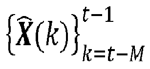
of extracted features ;
- taking said sequence of matrices 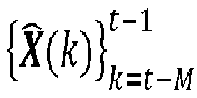
of extracted features and using a graph-based model to forecast desired signals 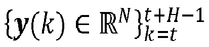
on an output network 
with a fixed number of third nodes N;
- interpolating said forecast desired signals so as to obtain forecasts of power resource production and/or consumption 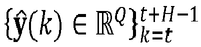
at at least one point of interest at at least one future point in time, where Q is the number of points of interest and H is the number of time steps in the future.
- obtaining past measurements v 1 , v 2 , ..., vN
- concatenating said past measurements v 1 , v 2 , ..., vN
- defining an intermediate network
- mapping said past measurements v 1 , v 2 , ..., vN
- taking said sequence of matrices
- interpolating said forecast desired signals so as to obtain forecasts of power resource production and/or consumption
Description
- The present invention relates to the field of distributed power networks. More particularly, it relates to a method of forecasting power production and/or consumption in a distributed power production and/or consumption network.
- As the percentage of decentralized renewable energy sources increases in an electricity distribution grid, the challenges to grid operators increases, particularly in respect of forecasting of the renewable energy production so as to be able to anticipate the usage of dispatchable energy sources such as conventional gas, coal, nuclear and hydroelectric production resources and thereby to keep the grid balanced.
- Typical state of the art approaches for renewable energy source production forecasting combine numerical weather predictions, satellite images and ground measurements with physical or machine learning models. However, such approaches tend to have low spatial and/or temporal resolution of the input data and thus of the resulting forecasts.
- Current approaches involve data from a fixed network of sensors (each sensor being situated at a node), and hence are only useful for producing forecasts of power production and/or consumption at the nodes, with basic interpolation producing low quality forecasts at other locations. In addition, when new nodes are introduced into the dataset (such as new rooftop photovoltaic systems), the entire forecasting calculation must be redone. Documents
US10425649 CN114154558 describe examples of such fixed network forecasting system which are subject to these drawbacks. - The aim of the present invention is hence to at least partially overcome the above-mentioned drawbacks of the prior art.
- More precisely, the invention relates to a method of forecasting weather-dependent power resource production and/or consumption, as defined in
independent claim 1. - This method can be carried out on a processing unit such as a general purpose computer and relates to a distributed power system comprising a time-varying plurality N k of first nodes at least some of which comprise of power resources adapted to produce and/or to consume power and which each comprise a sensor S 1,S 2, ...SN
k adapted to obtain direct or indirect measurements v 1,v 2,..., vNk of insolation and/or temperature at a plurality of timesteps M. Direct measurements can, for instance, be obtained from a weather station, whereas indirect measurements can be inferred from consumption of heating, lighting or cooling power of a building. - The method of the invention comprises steps of:
- obtaining past measurements v 1,v 2,...,vN
k from said sensors S 1, S 2 , ...SNk over time at times k; subsequently - concatenating said past measurements v 1 ,v 2 , ...,vN
k into a sequence of signal matrices
k were taken; subsequently - defining an
intermediate network 
- mapping said past measurements v 1 , v 2 , ..., vN
k from said sequence of signal matrices
intermediate network 

- taking said sequence of matrices


- interpolating said forecast desired signals so as to obtain forecasts of power resource production and/or consumption


- This method is robust to changes in the number of first nodes and the corresponding sensors, and does not need to be repeated in its entirety for every such change, or to make forecasts for new points of interest, i.e. for proposed new nodes. This significantly reduces the computing time and power required to carry it out compared to prior art methods.
- Advantageously, during said step of concatenating said past measurements v1, v2, ..., vN
k into a sequence of signal matrices
intermediate network 
intermediate network 
- Advantageously, said dynamic feature extraction comprises:
- carrying out feature embedding for each matrix X(k) and computing a fixed feature matrix

- stacking said matrices


- Advantageously, said sequence of matrices


- Advantageously, exogeneous variables {r(k)}, k = t, t + 1, ..., t + H are taken into account when generating said sequence of predicted variables of interest

- Advantageously, said at least one point of interest is not a node in the output network

- Further details of the invention will become more apparent upon reading the detailed description, in reference to the figures in which:
-
Figure 1 is a schematic representation of a distributed power system; -
Figure 2 is a schematic representation of the method according to the invention, in generic form; -
Figure 3 is a schematic representation of the steps of dynamic feature extraction in the second block B2 offigure 2 ; -
Figure 4 is a schematic representation of feature extraction, the forecast model and interpolation in blocks B2, B3 and B4 offigure 2 . -
Figure 1 illustrates schematically adistributed power system 1 upon which the method according to the invention can be carried out. - The
distributed power system 1 comprises a plurality of first nodes 3 (of which only a few have been indicated with a reference sign), at least some of which are linked with each other by a power distribution grid as is generally known. - At least some of said
first nodes 3 comprise a power resource arranged to produce and/or consume power, for instance photovoltaic arrays or wind turbines for producing power, and residential, commercial or industrial buildings which consume power. Eachfirst node 3 may have one or more power producing and/or power consuming entity associated with a sensor arranged to detect power generated or consumed. - Furthermore, some
first nodes 3 may additionally comprise, or may simply be, a weather station comprising a sensor adapted to measure solar irradiance and/or ambient temperature and/or wind speed. - As a result, each of said
first nodes 3 comprise or are associated with sensors S1, S2, ..., SNk arranged to measure quantities which vary according to the weather, whether directly in the case of a weather station or indirectly in the case of power generation or consumption. In essence, the power generation or consumption observations provide indirect information on the underlying weather phenomena, with sufficient correlation to be exploitable in the present method. The sensors S1, S2, ..., SNk can be considered as forming an input network. - The
first nodes 3 can be divided intoclusters 5 and local subgroups as indicated by dividing lines 7, and the location of each sensor is known in terms of at least its latitude and longitude. Its altitude can also be known. - The number of
first nodes 3 is not fixed, and can vary as power resources or weather stations are added to or removed from thepower distribution network 1, and this point is key to the invention: the method as described below is robust to such changes, and does not need to be repeated in its entirety for every change in thenetwork 1 or to make forecasts for proposednew nodes 3. For instance, the model can be updated to take into account new input data without any significant changes to the model architecture and without the need to retrain the models every time anew node 3 needs to be taken into consideration. - A processing unit, which may for instance be a general-purpose computer, distributed cloud computing or similar, carries out the method described below.
- The method of the invention uses graphs to model the spatio-temporal relations of the different signals in the system, that is to say weather station data, power generation or consumption data from various
first nodes 3. A "graph" in this context is a mathematical model that is composed of a set of nodes 3 (or vertices) and a set of edges that describe the relationship betweennodes 3. For example a weighted undirected graph can be defined as
first nodes 3 and ε is the set of edges (links). If nodes x i and x are connected, the edge between them is denoted as eij ∈ ε. The topology of the network (graph) is determined by the adjacency matrix A of size N × N. The matrix element Aij gives the edge weight between first nodes xi and xj and is zero in the absence of an edge eij . In the case of the invention, eachfirst node 3 represents a sensor, e.g. a power producing and/or consuming resource providing sensing data about power produced or consumed, or a weather station. The edges may represent the spatial proximity between stations or a learned relationship between them. - In the present invention, the number of first nodes N k in the network may vary at each discrete time k due to a disconnection of some power generation or consumption for example. Let

k (k) (time-series signals) of the sensor network S 1 , S 2 , ..., SNk for the past M discrete time samples, i.e., k = t - M, ..., t - 1. The method of the invention outputs forecasts of the desired signals (e.g. power generation or irradiance) for H time steps ahead, i.e. k = t,..., t + H - 1, in a set of points of interest (POI) defined by their geographical coordinates. The forecasting method is depicted inFigure 2 and it comprises four main blocks: the matrix formation block B1, the feature extraction block B2, the forecast block B3 and the interpolation block B4. - The first block B1 concatenates the measurement signals vi(k), i = 1, ...,Nk, into a matrix

first node 3 only measures a subset of the said variables, then a NaN (not a number) symbol is placed in the corresponding columns of the missing measurements. The number of measured variables F is fixed for all time steps. With this matrix representation, the input signals at time k = t can be described by the sequence of matrices
- The second block B2 is a graph feature extraction module that clusters the input nodes in

intermediate network 
first nodes 3. "Features" are characteristics of the data which provide useful information; in other words they are numerical values computed from the raw data which provide salient information about the data. The feature extraction block learns local node embeddings (features) for each node in the fixedintermediate network 
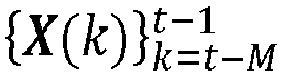


- The third block B3 is a forecast module, takes the features

intermediate network 


intermediate network 
- The fourth block B4 is an interpolation module which takes as inputs the forecasted signals

nodes 3, i.e. the points of interest (POI). The interpolation module forecasts the desired signals in the POI. The interpolation block uses graph-based methods that take into account the local and global topology of the input and output networks to produce the final forecasts on the desired nodes. -
Figure 3 illustrates a particular implementation example of the second block B2. - The first sub-block B21 of block B2 clusters all nodes at time k into
C clusters 5, whose centroids are predefined, and form the local feature matrices X i(k) ∈
cluster 5 with Nik denoting the numbers of nodes belonging to cluster i at time k. The first sub-block B21 also forms a local subgraph for each cluster by computing the matrices
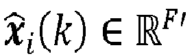

nodes 3 in the cluster. Examples of this function could be a weighted average, a graph attention network (see e.g. P. Veličković, G. Cucurull, A. Casanova, A. Romero, P. Lio, and Y. Bengio, 'Graph attention networks', International Conference on Learning Representations, 2018) or a self-attention graph pooling network (see e.g. J. Lee, I. Lee, and J. Kang, 'Self-Attention Graph Pooling', arXiv:1904.08082 [cs, stat], Jun. 2019, Accessed: Oct. 18, 2021. [Online]. Available: http://arxiv.org/abs/1904.08082). The third sub-block B23 stacks all vectors x̂i(k) into the fixed size matrix X (k). -
Figure 4 illustrates an implementation example of blocks B2, B3 and B4 of the method according to the invention. The input sequence
k (k) of the sensor network at past times, as described above in. Observations can for instance be generated or consumed power or solar irradiance. - Second block B2 uses a generic graph neural network (GNN) to implement the clustering and feature embedding as described above in the context of
figure 3 . - The feature extraction block B2 uses generic GNNs as the functions to implement the clustering B21 and feature aggregation B22 steps. In this implantation we assume that the C clusters and their centroids (fixed nodes in

For k = t - M,..., t: - 1. Assign a cluster to each node in

- 2. Form the local feature matrices { X i(k)}, i = 1, ..., C,
- 3. Form the local adjacency matrices { A i(k)}, i = 1, ..., C,
- 4. Compute xi (k)= f(Xi (k), Ai (k)),i=1,...,C,
- 5. Stack all xi (k),,i = 1, ..., C, into the fixed size matrix X (k).
- The local adjacency matrices A i(k) can be constructed using the k nearest neighbours algorithm of using a fully connected graph based on a function ofthe distance between nodes. Let Âi be the normalized adjacency matrix of thelocal subgraph at cluster i, defined as Âi=D̃i 1/2ÃiD̃1/2, where Ãi=Ai+IN
ik and D̃i is the degree matrix of Ãi. Possible candidates for the feature aggregation function f(·) are: - A) Weighted average. The feature vector can be computed as


- B) Graph attention network (see reference above). The feature vector is computed by the following steps:
- 1. z i(k) = softmax(Ai(k) X i (k) θ i)
- 2.

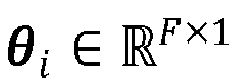

- C) Self-attention graph pooling network (see reference above). A variation of SAGPool can be used to compute the feature vector with the following steps:
- 1. zi (k)=tanh(Ai (k)Xi (k)θ i)
- 2. ki = argmax( zi (k))
- 3. xi(k) =[σ( Ai (k)Xi (k)Wi )] k
i :


- Note that the learnable parameters in all of the aforementioned functions are independent of Nik, i.e. are independent of the number of nodes at every cluster i and every time step k, thus independent of the number of input sensors at every time step.
- The forecasting module of block B3 is composed of an encoder-decoder model to forecast the desired variables (power or irradiance) at the N fixed locations defined in


where f in denotes the input number of features of matrix X, i.e. its number of columns, fout denotes the number output features from the graph convolution, i.e. the number of columns of Z, and, X (i) denotes the column vector formed by picking the i-th column of X. L is the graph Laplacian matrix of the underlying graph, defined as L = A - D, with D being the degree matrix of A, T k(·) denotes the Chebyshev polynomial of order k applied to each entry of a matrix, K denotes the order of the Chebyshev expansion, and,


- In the cell update equations sig(·) denotes the sigmoid function, ⊙ denotes the Hadmard product and tanh (·) denotes the hyperbolic tangent function. The weights W.,. and biases b. are learnable parameters whose dimensions are determined by the number of input and output features.
- The encoder block B31 uses GCLSTM cells to estimate the "hidden" cell state of the system given the past sequence {X̂(k)}, defined on fixed
graph 


- The interpolation block B4 takes the sequence {y(k)} and the locations (latitude and longitude) of the one or more POI as inputs and computes the forecasts on the POI. Without loss of generality we can suppose that the POI are all different from the locations in the fixed output network


- In the interpolation algorithm µ is a step size that controls the speed of the algorithm and β is the maximum eigen value of the matrix L ∇ ∇ T. The convergence criteria might a predefined number of iterations or until the solution doesn't change. The output forecasts

- The same methodology can also be used to make predictions of power consumption at points of interest.
- Although the invention has been described in terms of specific embodiments, variations thereto are possible without departing from the scope of the invention as defined by the appended claims.
Claims (7)
- Method of forecasting weather-dependent power resource production and/or consumption in a distributed power system (1) comprising a time-varying plurality N k of first nodes (3) at least some of which comprise of power resources adapted to produce and/or to consume power and which each comprise a sensor S 1 ,S 2 , ..., SN
k adapted to obtain direct or indirect measurements v 1 , v 2 , ..., vNk of insolation and/or temperature, at a plurality of past timesteps M, said method comprising the steps of :- obtaining past measurements v1, v2, ..., vNk from said sensors S 1, S 2, ..., SNk over time at times k,- concatenating said past measurements v1, v2, ..., vNk into a sequence of signal matrices - defining an intermediate network
 - mapping said past measurements v1, v2, ..., vN
k from said sequence of signal matrices

 - taking said sequence of matrices

 - interpolating said forecast desired signals so as to obtain forecasts of power resource production and/or consumption
- Method according to claim 1, wherein, during said step of concatenating said past measurements v1, v2, ..., vN
k into a sequence of signal matrices


- Method according to claim 1 or 2, wherein said dynamic feature extraction comprises:- carrying out feature embedding for each matrix X(k) and computing a fixed feature matrix
 - stacking said matrices

- Method according to claim 3, wherein said sequence of matrices


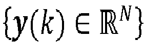
- Method according to any preceding claim, wherein exogeneous variables { r (k)}, k = t, t + 1, ...,t + H are taken into account when generating said sequence of predicted variables of interest
- Method according to any preceding claim, wherein said at least one point of interest is not a third node in the output network

- Computer program product comprising instructions which, when the program is executed by a computer, cause the computer to carry out the steps of the method of any preceding claim.
Priority Applications (1)
| Application Number | Priority Date | Filing Date | Title |
|---|---|---|---|
| EP22211594.1A EP4383498A1 (en) | 2022-12-06 | 2022-12-06 | Method of forecasting power production/consumption in a distributed network |
Applications Claiming Priority (1)
| Application Number | Priority Date | Filing Date | Title |
|---|---|---|---|
| EP22211594.1A EP4383498A1 (en) | 2022-12-06 | 2022-12-06 | Method of forecasting power production/consumption in a distributed network |
Publications (1)
| Publication Number | Publication Date |
|---|---|
| EP4383498A1 true EP4383498A1 (en) | 2024-06-12 |
Family
ID=84440058
Family Applications (1)
| Application Number | Title | Priority Date | Filing Date |
|---|---|---|---|
| EP22211594.1A Pending EP4383498A1 (en) | 2022-12-06 | 2022-12-06 | Method of forecasting power production/consumption in a distributed network |
Country Status (1)
| Country | Link |
|---|---|
| EP (1) | EP4383498A1 (en) |
Cited By (2)
| Publication number | Priority date | Publication date | Assignee | Title |
|---|---|---|---|---|
| CN118644359A (en) * | 2024-08-16 | 2024-09-13 | 山东省计算中心(国家超级计算济南中心) | Hydrogen energy load prediction method and system applied to industrial parks |
| CN120910514A (en) * | 2025-10-11 | 2025-11-07 | 鲁东大学 | Multivariable time sequence prediction method and device based on space-time feature fusion |
Citations (2)
| Publication number | Priority date | Publication date | Assignee | Title |
|---|---|---|---|---|
| US10425649B2 (en) | 2014-10-21 | 2019-09-24 | Lg Electronics Inc. | Method and apparatus for performing graph-based prediction using optimization function |
| CN114154558A (en) | 2021-11-12 | 2022-03-08 | 山东浪潮科学研究院有限公司 | Distributed energy power generation load prediction system and method based on graph neural network |
-
2022
- 2022-12-06 EP EP22211594.1A patent/EP4383498A1/en active Pending
Patent Citations (2)
| Publication number | Priority date | Publication date | Assignee | Title |
|---|---|---|---|---|
| US10425649B2 (en) | 2014-10-21 | 2019-09-24 | Lg Electronics Inc. | Method and apparatus for performing graph-based prediction using optimization function |
| CN114154558A (en) | 2021-11-12 | 2022-03-08 | 山东浪潮科学研究院有限公司 | Distributed energy power generation load prediction system and method based on graph neural network |
Non-Patent Citations (7)
| Title |
|---|
| ESCHENBACH ANNETTE ET AL: "Spatio-Temporal Resolution of Irradiance Samples in Machine Learning Approaches for Irradiance Forecasting", IEEE ACCESS, IEEE, USA, vol. 8, 12 March 2020 (2020-03-12), pages 51518 - 51531, XP011779563, DOI: 10.1109/ACCESS.2020.2980775 * |
| J. LEEI. LEEJ. KANG: "Self-Attention Graph Pooling", ARXIV.R904.08082, June 2019 (2019-06-01) |
| JELENA SIMEUNOVI\'C ET AL: "Spatio-temporal graph neural networks for multi-site PV power forecasting", ARXIV.ORG, CORNELL UNIVERSITY LIBRARY, 201 OLIN LIBRARY CORNELL UNIVERSITY ITHACA, NY 14853, 1 November 2021 (2021-11-01), XP091089956 * |
| P. VELICKOVICG. CUCURULLA. CASANOVAA. ROMEROP. LIOY. BENGIO: "Graph attention networks", INTERNATIONAL CONFERENCE ON LEAMING REPRESENTATIONS, 2018 |
| PRADO-RUJAS IGNACIO-IKER ET AL: "A Flexible and Robust Deep Learning-Based System for Solar Irradiance Forecasting", IEEE ACCESS, IEEE, USA, vol. 9, 14 January 2021 (2021-01-14), pages 12348 - 12361, XP011833648, DOI: 10.1109/ACCESS.2021.3051839 * |
| RICHARD HEADEN INMAN: "Solar forecasting review", MSC. THESIS IN ENGINEERING SCIENCES, 1 January 2012 (2012-01-01), XP055157531, Retrieved from the Internet <URL:https://escholarship.org/uc/item/7zv8s0w9.pdf> [retrieved on 20141209] * |
| SIMEUNOVIC, BSCHUBNEL, P.-J. ALETR. E. CARRILLO: "Spatio-Temporal Graph Neural Networks for Multi-Site PV Power Forecasting", IEEE TRANSACTIONS ON SUSTAINABLE ENERGY, vol. 13, no. 2, 2022, pages 1210 - 1220 |
Cited By (3)
| Publication number | Priority date | Publication date | Assignee | Title |
|---|---|---|---|---|
| CN118644359A (en) * | 2024-08-16 | 2024-09-13 | 山东省计算中心(国家超级计算济南中心) | Hydrogen energy load prediction method and system applied to industrial parks |
| CN120910514A (en) * | 2025-10-11 | 2025-11-07 | 鲁东大学 | Multivariable time sequence prediction method and device based on space-time feature fusion |
| CN120910514B (en) * | 2025-10-11 | 2026-01-06 | 鲁东大学 | A Multivariate Time Series Prediction Method and Apparatus Based on Spatiotemporal Feature Fusion |
Similar Documents
| Publication | Publication Date | Title |
|---|---|---|
| Limouni et al. | Accurate one step and multistep forecasting of very short-term PV power using LSTM-TCN model | |
| Cheng et al. | Multi-meteorological-factor-based graph modeling for photovoltaic power forecasting | |
| Wang et al. | A comparison of day-ahead photovoltaic power forecasting models based on deep learning neural network | |
| Marinho et al. | Short-term solar irradiance forecasting using CNN-1D, LSTM, and CNN-LSTM deep neural networks: A case study with the Folsom (USA) dataset | |
| Ghaderi et al. | Deep forecast: Deep learning-based spatio-temporal forecasting | |
| Dewangan et al. | Combining forecasts of day-ahead solar power | |
| Rana et al. | 2D-interval forecasts for solar power production | |
| Chen et al. | Online 24-h solar power forecasting based on weather type classification using artificial neural network | |
| Moradzadeh et al. | A novel cyber-Resilient solar power forecasting model based on secure federated deep learning and data visualization | |
| Wang et al. | An approach for day-ahead interval forecasting of photovoltaic power: A novel DCGAN and LSTM based quantile regression modeling method | |
| CN116706888A (en) | Load forecasting method for smart grid based on federated learning | |
| Alimohammadi et al. | Multi-stage algorithm for uncertainty analysis of solar power forecasting | |
| CN119646636A (en) | A wind power prediction method and system based on multiple time scales | |
| Mohanty et al. | Artificial intelligence based forecasting & optimization of solar cell model | |
| Yang et al. | Research on distributed photovoltaic power prediction based on spatiotemporal information ensemble method | |
| Zjavka | Wind speed and global radiation forecasting based on differential, deep and stochastic machine learning of patterns in 2-level historical meteo-quantity sets | |
| CN119340995A (en) | A distributed photovoltaic power prediction method, device, equipment, medium and product | |
| Yu et al. | Multi-site solar irradiance prediction based on hybrid spatiotemporal graph neural network | |
| CN118713054A (en) | A method, device, equipment and medium for training a power generation prediction model | |
| Zhang et al. | Multi-step ahead forecasting of wind vector for multiple wind turbines based on new deep learning model | |
| Singhal et al. | Solar-cast: solar power generation prediction from weather forecasts using machine learning | |
| Yang et al. | An improved spatial upscaling method for producing day‐ahead power forecasts for wind farm clusters | |
| Junhuathon et al. | Deep-learning-based short-term photovoltaic power generation forecasting using improved self-organization map neural network | |
| Zhang et al. | County-level distributed PV day-ahead power prediction based on grey correlation analysis and transformer-GCAN model | |
| El Marghichi | A Solar PV Model Parameter Estimation Based on the Enhanced Self-Organization Maps |
Legal Events
| Date | Code | Title | Description |
|---|---|---|---|
| PUAI | Public reference made under article 153(3) epc to a published international application that has entered the european phase |
Free format text: ORIGINAL CODE: 0009012 |
|
| STAA | Information on the status of an ep patent application or granted ep patent |
Free format text: STATUS: THE APPLICATION HAS BEEN PUBLISHED |
|
| AK | Designated contracting states |
Kind code of ref document: A1 Designated state(s): AL AT BE BG CH CY CZ DE DK EE ES FI FR GB GR HR HU IE IS IT LI LT LU LV MC ME MK MT NL NO PL PT RO RS SE SI SK SM TR |
|
| STAA | Information on the status of an ep patent application or granted ep patent |
Free format text: STATUS: REQUEST FOR EXAMINATION WAS MADE |
|
| 17P | Request for examination filed |
Effective date: 20241209 |