EP4345696A1 - Data processing apparatus, program, and data processing method - Google Patents
Data processing apparatus, program, and data processing method Download PDFInfo
- Publication number
- EP4345696A1 EP4345696A1 EP23194811.8A EP23194811A EP4345696A1 EP 4345696 A1 EP4345696 A1 EP 4345696A1 EP 23194811 A EP23194811 A EP 23194811A EP 4345696 A1 EP4345696 A1 EP 4345696A1
- Authority
- EP
- European Patent Office
- Prior art keywords
- state
- value
- state variable
- values
- searching
- Prior art date
- Legal status (The legal status is an assumption and is not a legal conclusion. Google has not performed a legal analysis and makes no representation as to the accuracy of the status listed.)
- Pending
Links
Images


Classifications
-
- G—PHYSICS
- G06—COMPUTING OR CALCULATING; COUNTING
- G06F—ELECTRIC DIGITAL DATA PROCESSING
- G06F17/00—Digital computing or data processing equipment or methods, specially adapted for specific functions
- G06F17/10—Complex mathematical operations
- G06F17/18—Complex mathematical operations for evaluating statistical data, e.g. average values, frequency distributions, probability functions, regression analysis
-
- G—PHYSICS
- G06—COMPUTING OR CALCULATING; COUNTING
- G06N—COMPUTING ARRANGEMENTS BASED ON SPECIFIC COMPUTATIONAL MODELS
- G06N5/00—Computing arrangements using knowledge-based models
- G06N5/01—Dynamic search techniques; Heuristics; Dynamic trees; Branch-and-bound
-
- G—PHYSICS
- G06—COMPUTING OR CALCULATING; COUNTING
- G06F—ELECTRIC DIGITAL DATA PROCESSING
- G06F17/00—Digital computing or data processing equipment or methods, specially adapted for specific functions
- G06F17/10—Complex mathematical operations
- G06F17/11—Complex mathematical operations for solving equations, e.g. nonlinear equations, general mathematical optimization problems
-
- G—PHYSICS
- G06—COMPUTING OR CALCULATING; COUNTING
- G06N—COMPUTING ARRANGEMENTS BASED ON SPECIFIC COMPUTATIONAL MODELS
- G06N7/00—Computing arrangements based on specific mathematical models
- G06N7/01—Probabilistic graphical models, e.g. probabilistic networks
Definitions
- the embodiment discussed herein relates to a data processing apparatus, program, and data processing method.
- the Markov chain Monte Carlo method is hereinafter abbreviated as MCMC method.
- processing by the MCMC method may be referred to as MCMC processing.
- MCMC processing a state transition is accepted with an acceptance probability of the state transition defined, for example, by a Metropolis or Gibbs method.
- Simulated annealing and replica exchange are optimization or sampling methods which can be used with MCMC methods.
- the number of coefficients defining a problem increases with an increase in the scale of the problem.
- the scale of the problem is represented by the number of state variables, which corresponds to the number of spins of the Ising model.
- bias may occur in the solution search range for each partial neighbor (i.e., each divided state variable group). In this case, an efficient solution search may fail.
- One aspect of the embodiment is to provide a data processing apparatus, program, and data processing method that enable an efficient solution search.
- a data processing apparatus including: first memory means for storing values of a plurality of weight coefficients included in an evaluation function which is obtained by transforming a combinatorial optimization problem; second memory means for storing, amongst the plurality of weight coefficients, values of a weight coefficient group which is associated with a state variable group selected from a plurality of state variable groups, the plurality of state variable groups being obtained by dividing a plurality of state variables included in the evaluation function; searching means for searching for a solution to the combinatorial optimization problem by repeating an update process, the update process including a process of calculating, using the values of the weight coefficient group read from the second memory means, a change in a value of the evaluation function responsive to changing a value of each of state variables of the state variable group and a process of changing a value of one of the state variables of the state variable group based on the change and a temperature value; and processing means for calculating, based on the change and the temperature value, multiplicity indicating a number of iterations in
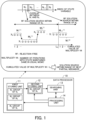
- FIG. 1 illustrates an example of a data processor according to the present embodiment.
- a data processor 10 searches for a solution to a combinatorial optimization problem by Rejection-Free using, for example, simulated annealing or replica exchange and outputs the found solution.
- the combinatorial optimization problem is transformed, for example, into an Ising-type evaluation function.
- the evaluation function is also called objective function or energy function.
- the evaluation function includes multiple state variables and multiple weight coefficients.
- the state variables are binary variables whose only possible values are 0 and 1. Each state variable may be represented using a bit. Solutions to the combinatorial optimization problem are represented by the values of the multiple state variables. A solution that minimizes the value of the evaluation function corresponds to the optimal solution of the combinatorial optimization problem.
- the value of the evaluation value is referred to as energy.
- E x ⁇ ⁇ ⁇ i , j ⁇ W ij x i x j ⁇ ⁇ i b i x i
- Equation (1) is an evaluation function formulated in quadratic unconstrained binary optimization (QUBO) format. In the case of a problem of maximizing the energy, the sign of the evaluation function is reversed.
- QUBO quadratic unconstrained binary optimization
- the first term on the right side of equation (1) is a summation of the products of the values of two state variables and their weight coefficient for all mutually exclusive and collectively exhaustive combinations of two state variables selectable from all state variables.
- Subscripts i and j are indices of the state variables.
- x i denotes the i-th state variable and x j denotes the j-th state variable.
- the number of state variables is n, the number of W ij is n ⁇ n.
- Equation (1) The second term on the right side of equation (1) is a summation of the products of the bias of each of all the state variables and the value of the state variable.
- b i denotes the bias of the i-th state variable.
- h i is referred to as local field (LF).
- LF local field
- a Metropolis or Gibbs method is used to determine whether to accept a state transition with an energy change of ⁇ E i , that is, a change of the value of the state variable x i .
- a neighbor search that searches for a transition from a current state to a different state with an energy lower than that of the current state, not only a transition to a state with lower energy but also a transition to a state with higher energy is stochastically accepted.
- an acceptance probability A i of accepting a change in the value of the state variable that causes ⁇ E i is defined by equation (3) below.
- a i ⁇ min 1 , exp ⁇ ⁇ ⁇ E i METROPOLIS METHOD 1 / 1 + exp ⁇ ⁇ E i GIBBS METHOD
- T is also referred to as temperature values hereinafter.
- the min operator returns the minimum value of its arguments.
- the upper part and lower part on the right side of equation (3) correspond to the Metropolis method and the Gibbs method, respectively.
- n ⁇ n W ij 's are used for the calculation of ⁇ E 1 to ⁇ E n .
- the W ij 's are not storable in fast but relatively small-capacity memory (e.g., on-chip memory).
- the W ij 's are stored in memory with relatively large capacity (e.g., dynamic random-access memory (DRAM)).
- DRAM dynamic random-access memory
- the access time of a DRAM is, for example, about two orders of magnitude greater than that of an on-chip random access memory (RAM), which therefore greatly limits the processing speed.
- the data processor 10 of the present embodiment performs neighbor searches using multiple state variable groups obtained by dividing the n state variables.
- Each of the multiple state variable groups is hereinafter referred to as a partial neighbor.
- the data processor 10 includes a first storing unit 11, a second storing unit 12, a searching unit 13, and a processing unit 14.
- the first storing unit 11 stores therein the values of multiple weight coefficients included in an evaluation function, which is obtained by transforming a combinatorial optimization problem.
- the first storing unit 11 stores multiple weight coefficients divided into weight coefficient groups, each of which is associated with one of the multiple partial neighbors.
- the first storing unit 11 is, for example, a storage device which is slower but has a larger capacity than the second storing unit 12 to be described later.
- Examples of such a storage device include a volatile electronic circuit, such as a DRAM, and a non-volatile electronic circuit, such as a hard disk drive (HDD) and flash memory.
- a volatile electronic circuit such as a DRAM
- a non-volatile electronic circuit such as a hard disk drive (HDD) and flash memory.
- the multiple partial neighbors are generated in such a manner that the weight coefficient group associated with each partial neighbor may be stored in the second storing unit 12.
- the multiple partial neighbors may be generated by the processing unit 14 of the data processor 10 based on problem information (including indices of the n state variables and the n ⁇ n W ij 's) stored in the first storing unit 11 or a different storage device.
- a device external to the data processor 10 may generate the multiple partial neighbors.
- each partial neighbor represents a part (subset) of state space represented by the values of x i to x n ; (2) each partial neighbor is part of the whole neighbor; (3) if state Y is a partial neighbor of state X, then state X is also a partial neighbor of state Y; and (4) the probability of transition within a partial neighbor is proportional to that within the whole neighbor, and the probability of transition out of the partial neighbor is zero.
- the transition probability is given by the product of a proposal probability and the acceptance probability A i of equation (3).
- state X is a partial neighbor of state Y even if state Y is obtained from state X via multiple state transitions to partial neighbors.
- multiple partial neighbors are generated, for example, by simply dividing x 1 to x n in order of indices.
- the multiple partial neighbors may also be generated by randomly selecting the indices and dividing x 1 to x n such that each partial neighbor contains approximately the same number of state variables.
- duplicate indices may be included in each partial neighbor. It is, however, preferable that each index be included in at least one partial neighbor. Note that, after a solution search is performed for each of the multiple partial neighbors, or after a solution search for each partial neighbor is repeated several times, indices may be randomly selected again so as to generate multiple partial neighbors and perform solution searches.
- the method of generating multiple partial neighbors is not limited to the method described above.
- all combinations of two indices i and j, i.e., (1, 2), ..., (1, n), (2, 3), (2, 4), ..., (2, n), ..., and (n-1, n) may be set as a whole neighbor, which is then divided into multiple partial neighbors.
- FIG. 1 depicts an example where n state variables are divided into I partial neighbors (N 2 to N 1 ). Taking a neighbor of one bit flipping as an example, each of N 1 to N I is defined by a set of indices of state variables to be flipped.
- j i (i) represents the i-th index amongst the indices of the m state variables included in N i .
- different partial neighbors may contain the same indices, as illustrated in FIG. 1 . That is, the ranges of indices included may overlap between different partial neighbors.
- the first storing unit 11 stores therein groups of weight variables (W ij 's) associated with the individual partial neighbors.
- the W ij group of N 1 includes weight coefficients between, amongst the n state variables, each of the state variables included in N 1 and the rest of the state variables of N 1 .
- the W ij group of N 2 includes weight coefficients between, amongst the n state variables, each of the state variables included in N 2 and the rest of the state variables of N 2 .
- the W ij group of N I includes weight coefficients between, amongst the n state variables, each of the state variables included in N T and the rest of the state variables of N I .
- the first storing unit 11 may also store various programs, such as a program that causes the data processor 10 to search for solutions to combinatorial optimization problems, and various data.
- the second storing unit 12 stores therein, amongst the multiple weight coefficients included in the evaluation function, a weight coefficient group associated with a partial neighbor selected from the multiple partial neighbors.
- the second storing unit 12 is, for example, a storage device that is faster but has a smaller capacity than the above-described first storing unit 11. Examples of such a storage device include a volatile electronic circuit, such as a static random-access memory (SRAM).
- the second storing unit 12 may include an electronic circuit, such as a register.
- the searching unit 13 performs a solution search for each partial neighbor (corresponding to the above-described sub-problem).
- the searching unit 13 reads the weight coefficient group stored in the second storing unit 12.
- the searching unit 13 uses the read weight coefficient group to calculate a change ( ⁇ E i ) in the value of the evaluation function, made by changing the value of each state variable of the selected partial neighbor.
- ⁇ E i is given, for example, by equation (2).
- the value of each state variable, the local field, the energy, and the like included in equation (2) are stored in a storing unit (e.g., a storage circuit, such as a register) (not illustrated) provided in the searching unit 13.
- the searching unit 13 is able to calculate in parallel ⁇ E i 's for the individual state variables of the selected partial neighbor.
- the searching unit 13 changes the value of one state variable of the partial neighbor, based on ⁇ E i 's for the individual state variables and a temperature value.
- the searching unit 13 performs a solution search by Rejection-Free.
- Rejection-Free one of the state variables included in the partial neighbor is selected based on the probability given by the following equation (4), which uses the acceptance probability A i defined by equation (3), and the value of the selected state variable is changed.
- m is the number of state variables included in the selected state variable group.
- Equation (4) The selection based on the probability given by equation (4) is equivalent to selecting the state variable with an index of j defined by the following equation (5).
- j argmin i max 0 , ⁇ E i + T ln ⁇ ln r i argmin i indicates i with the minimum argument.
- the searching unit 13 updates the local field and energy stored in a register or the like.
- the searching unit 13 searches for a solution to a combinatorial optimization problem by repeating, for each partial neighbor selected by the processing unit 14, an update process (including updates of the local field and energy) that includes the process of calculating ⁇ E i and the process of changing the value of a state variable.
- the searching unit 13 described above may be implemented using an electronic circuit, such as an application specific integrated circuit (ASIC) or field programmable gate array (FPGA).
- the searching unit 13 may be implemented through software processing in which a program is executed by a hardware processor, such as a central processing unit (CPU), graphics processing unit (GPU), or digital signal processor (DSP).
- CPU central processing unit
- GPU graphics processing unit
- DSP digital signal processor
- the processing unit 14 calculates multiplicity, which is the number of iterations in which a state remains in the same state using a usual MCMC method instead of Rejection-Free.
- ⁇ X n ⁇ ⁇ a, b, b, b, a, a, c, c, c, c, d, d, ... ⁇ .
- original chain the time series of states obtained in the solution search using the usual MCMC method
- the multiplicity may also be said to be the number of samples of the original chain per sample obtained in the solution search by Rejection-Free.
- the processing unit 14 calculates the multiplicity (M) based on the following equation (6).
- M 1 + ⁇ ln r / ln 1 ⁇ P e ⁇
- Equation (6) square brackets represent a floor function.
- r is a uniform random number value between 0 and 1.
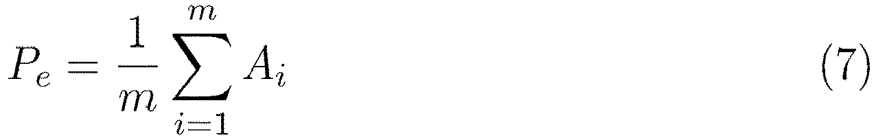
- P e represents the probability of the state changing in one iteration and is called escape probability.
- the multiplicity M is a random variable following the geometric distribution of P e , and a random number following the distribution is generated by equation (6).
- P e is given by the following equation (7).
- the processing unit 14 When the cumulated value of the multiplicity exceeds a predetermined threshold, the processing unit 14 causes the searching unit 13 to perform an update process using the weight coefficient group associated with a different partial neighbor selected from the multiple partial neighbors. For example, when the cumulated value of the multiplicity exceeds the predetermined threshold, the processing unit 14 selects an unselected partial neighbor from the multiple partial neighbors, then reads the values of a weight coefficient group associated with the partial neighbor from the first storing unit 11, and stores (writes) the read values of the weight coefficient group in the second storing unit 12. For example, the processing unit 14 overwrites the original weight coefficient group values with the values of the weight coefficient group associated with the newly selected partial neighbor.
- the processing unit 14 may select another partial neighbor in advance and store, in the second storing unit 12, the values of the weight coefficient group associated with the selected partial neighbor (see FIG. 8 described later).
- the processing unit 14 has the function of a controller that controls each unit of the data processor 10.
- the processing unit 14 may be implemented using an electronic circuit, such as an ASIC or FPGA. Alternatively, the processing unit 14 may be implemented through software processing in which a program is executed by a hardware processor, such as a CPU, GPU, or DSP.
- a hardware processor such as a CPU, GPU, or DSP.
- FIG. 1 depicts an example of a solution search by the data processor 10, described above.
- the searching unit 13 performs a solution search within the range of N 1 by Rejection-Free.
- state transitions start from state X 0 and then take place in the order of states X 1 , X 2 , ..., and X 1 .
- state X 0 is repeated for three iterations
- state X 1 is repeated for six iterations
- state X 2 is repeated for three iterations. That is, the multiplicity (M 2 (1) ) of state X 0 is 3, the multiplicity (M 2 (1) ) of state X 1 is 6, and the multiplicity (M 3 (1) ) of state X 2 is 3.
- the processing unit 14 calculates the multiplicity based on the above equation (6), and also determines whether the cumulated value exceeds a predetermined threshold. In the example of FIG. 1 , when the multiplicity of state X l has reached 3, the cumulated value exceeds the threshold (L 0 ). Therefore, the processing unit 14 selects a different partial neighbor (N 2 in the example of FIG. 1 ), then reads the values of a weight coefficient group associated with the partial neighbor (the values of W ij group of N 2 ) from the first storing unit 11 and stores them in the second storing unit 12.
- the solution search within the range of N 2 using Rejection-Free starts from state X l .
- the processing unit 14 again repeats the calculation of the multiplicity and the determination of whether the cumulated value exceeds the threshold.
- the multiplicity of X l within the range of N 2 is denoted by M 1 (2) .
- the data processor 10 may function as a sampling device.
- the probability distribution indicating the probability of occupancy of each state in an equilibrium state is a target distribution (e.g., a Boltzmann distribution). Therefore, by outputting, as samples, states obtained in the process of repeating state transitions or values based on the obtained states, samples following the target distribution are acquired. The acquired samples are used, for example, to calculate an expected value in machine learning or the like.
- a target distribution e.g., a Boltzmann distribution
- the searching unit 13 outputs the values of multiple state variables for each update process (i.e., for each iteration of Rejection-Free), for example, as a sample.
- the processing unit 14 outputs the multiplicity M for the values of the multiple state variables (i.e., for each state).
- the target distribution is obtained by weighting the sample according to the multiplicity M.
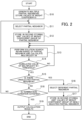
- FIG. 2 is a flowchart illustrating a general flow of the data processing method.
- step S10 based on problem information of a combinatorial optimization problem in question, partial neighbors are generated by the method described above (step S10).
- the multiple partial neighbors may be generated by the processing unit 14 or a device external to the data processor 10.
- the values of multiple weight coefficients included in a corresponding evaluation function are stored in the first storing unit 11.
- the processing unit 14 selects a partial neighbor to be a solution search target (step S11), and stores the values of a weight coefficient group associated with the selected partial neighbor in the second storing unit 12 (step S12).
- the searching unit 13 performs a solution search within the range of the partial neighbor, using the values of the weight coefficient group stored in the second storing unit 12 (step S13). Further, in step S13, the processing unit 14 calculates the multiplicity M.
- the processing unit 14 determines whether the cumulated value of the multiplicity M exceeds a predetermined threshold (L 0 in the above example) (step S14). If determining that the cumulated value does not exceed the threshold, the processing unit 14 returns to step S13.
- the processing unit 14 determines whether there is a partial neighbor yet to be selected (step S15). If determining that there is an unselected partial neighbor, the processing unit 14 moves to step S16. If not, the processing unit 14 moves to step S18.
- step S16 the processing unit 14 selects a partial neighbor yet to be selected. Then, the processing unit 14 stores, in the second storing unit 12, the values of a weight coefficient group associated with the newly selected partial neighbor (step S17). Subsequently, the processing unit 14 repeats the process starting from step S13.
- step S18 the processing unit 14 determines whether a condition for terminating the solution search is satisfied.
- the condition for terminating the solution search may be, for example, whether the number of iterations has reached a predetermined number. In the case of using simulated annealing, the termination condition is, for example, whether the temperature value has reached a final temperature value. If determining that the termination condition is not satisfied, the processing unit 14 repeats the process starting from step 511.
- the processing unit 14 may repeat the process starting from step S10 instead when determining that the termination condition is not satisfied. In this case, the processing unit 14 may generate multiple partial neighbors using a method different from the previous one.
- the processing unit 14 When determining that the termination condition is satisfied, the processing unit 14 outputs calculation results (step S19) and terminates the processing.
- the calculation results are, for example, a state (the values of x 1 to x n ) with the lowest energy obtained, amongst energies obtained in the update processes.
- FIG. 3 is a flowchart illustrating an example of procedures for a partial neighbor solution search and sampling.
- the following processing is performed, for example, while gradually decreasing a temperature value T from a start value to an end value according to a predetermined temperature change schedule.
- the temperature value T is reduced by multiplying the temperature value T by a value smaller than 1 for each fixed number of iterations.
- the following processing is performed while gradually increasing the temperature value T.
- the searching unit 13 uses multiple replica circuits each having a different temperature value. Each replica circuit searches for a solution using the same partial neighbor. Then, the following processing is performed in each of the replica circuits.
- the processing unit 14 exchanges replicas each time a predetermined number of iterations is repeated. For example, the processing unit 14 randomly selects a pair of replica circuits with adjacent temperature values amongst the multiple replica circuits, and exchanges the temperature values or states between the two selected replica circuits, with an exchange probability based on their energy or temperature difference.
- the processing unit 14 first performs an initialization process (step S20).
- the initialization process includes setting of the following items: initial values of the energy and local field; the aforementioned threshold (L 0 ); the total number of partial neighbors (K in the example below); a condition for terminating the solution search (an upper limit Itr of the number of iterations in the example below).
- the simulated annealing method is performed, the followings are also set: the start value and the end value of T (or ⁇ ); and the value by which T (or ⁇ ) is multiplied for each predetermined temperature change cycle.
- the replica exchange method is performed, a temperature value for each replica circuit is set.
- the processing unit 14 determines whether M ⁇ L (step S24).
- the process of step S24 corresponds to that of step S14 of determining whether the cumulated value of the multiplicity M exceeds the threshold, depicted in FIG. 2 . If determining that M ⁇ L, the processing unit 14 moves to step S25. If not, the processing unit 14 moves to step S27.
- step S25 the processing unit 14 assigns L - M to L. Then, the processing unit 14 causes the searching unit 13 to update the state based on ⁇ E i calculated in step S23 and the temperature value (step S26).
- the state update is done by changing the value of one state variable of the partial neighbor, selected by the aforementioned Rejection-Free. With the state update, the local field and energy are also updated. In addition, when the updated energy is the lowest ever, the searching unit 13 may hold the value of the lowest energy and the state with the lowest energy.
- step S26 the processing unit 14 outputs (or stores in a storing unit not illustrated) the state before the update and the multiplicity M calculated for the state before the update.
- step S26 the processing unit 14 repeats the process starting from step S23.
- step S27 the processing unit 14 outputs (or stores in a storing unit not illustrated) a sample (here, including the current state and L as the multiplicity of the state). No state update takes place in step S27.
- step S27 the processing unit 14 determines whether k ⁇ K (step S28). If determining that k ⁇ K, the processing unit 14 moves to step S30. If not, the processing unit 14 moves to step S29.
- step S29 the processing unit 14 assigns k + 1 to k so as to switch the solution search target to the next partial neighbor. Subsequently, the processing unit 14 repeats the process starting from step S22.
- step S30 the processing unit 14 determines whether itr ⁇ Itr, where itr is a variable representing the number of iterations and has an initial value of 1. If determining that itr ⁇ Itr, the processing unit 14 moves to step S31. If not, the processing unit 14 moves to step S32.
- step S31 the processing unit 14 assigns itr + 1 to itr. Subsequently, the processing unit 14 repeats the process starting from step S21.
- the process of step S32 is the same as that of step S19 of FIG. 2 .
- processing order illustrated in FIGS. 2 and 3 is merely an example, and the order may be changed as appropriate.
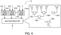
- FIG. 4 illustrates a circuit example for selecting a state variable whose value is to be changed by Rejection-Free.
- the searching unit 13 includes k i calculation circuits 13a1, 13a2, ..., and 13am and a selection circuit unit 13b used to select a state variable whose value is to be changed by Rejection-Free.
- the selection circuit unit 13b includes multiple selection circuits (selection circuits 13b1, 13b2, 13b3, 13b4, 13b5 and so on) arranged over multiple levels in a tree like structure.
- Each of the multiple selection circuits outputs the smaller of the two k i 's and its index. When the values of the two k i 's are equal, k i with the smaller index and the index are output.
- the index (j) output from the selection circuit 13b5 at the lowest level is j of equation (5), which is the index of a state variable whose value is to be changed.
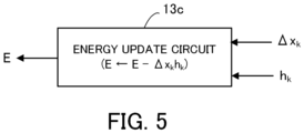
- FIG. 5 illustrates an update of energy
- the searching unit 13 includes an energy update circuit 13c depicted in FIG. 5 .
- the energy update circuit 13c updates the energy based on the change ⁇ x k and h k , which is the local field of x k .
- the energy E is updated by subtracting ⁇ x k h k from the original energy E.
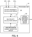
- FIG. 6 illustrates an example of a processing unit.
- the processing unit 14 includes an escape probability calculation circuit 20, a multiplicity calculation circuit 21, a uniform random number generation circuit 22, and a partial neighbor switching determination circuit 23.
- the escape probability calculation circuit 20 receives ⁇ E 1 , ⁇ E 2 , ..., and ⁇ E m output from the searching unit 13. Then, the escape probability calculation circuit 20 calculates the escape probability P e given by the above equation (7).
- the multiplicity calculation circuit 21 calculates the multiplicity M given by the above equation (6) based on P e calculated by the escape probability calculation circuit 20 and a uniform random number r.
- the uniform random number generation circuit 22 generates the uniform random number r between 0 and 1.
- the uniform random number generation circuit 22 is implemented using, for example, a Mersenne Twister, linear feedback shift register (LFSR), or the like.
- the partial neighbor switching determination circuit 23 switches a partial neighbor on which the searching unit 13 performs a solution search when the cumulated value of the multiplicity M exceeds a threshold (L 0 in the example of FIG. 1 ).
- Equation (7) is given by the above equation (7), as described above. Further, equation (7) may be expanded as the following equation (8).
- P e defined as equation (8) is calculated by the escape probability calculation circuit 20 described below.
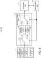
- FIG. 7 illustrates an example of the escape probability calculation circuit.
- the escape probability calculation circuit 20 includes ⁇ i calculation circuits 20a1, 20a2, ..., and 20am, A i calculation circuits 20b1, 20b2, ..., and 20bm, an addition circuit 20c, a register 20d, and a multiplication circuit 20e.
- Each of the ⁇ i calculation circuits 20a1 to 20am calculates ⁇ i given by equation (9) based on ⁇ E i and ⁇ (inverse temperature) .
- the ⁇ i calculation circuit 20a1 calculates ⁇ 1 ; the ⁇ i calculation circuit 20a2 calculates ⁇ 2 ; and the ⁇ i calculation circuit 20am calculates ⁇ m .
- the A i calculation circuit 20b1 calculates exp(- ⁇ 1 ); the A i calculation circuit 20b2 calculates exp(- ⁇ 2 ); and the A i calculation circuit 20bm calculates exp(- ⁇ m ).
- the addition circuit 20c adds up exp(- ⁇ 1 ) to exp(- ⁇ m ).
- the register 20d holds and outputs the addition results output from the addition circuit 20c in synchronization with a clock signal.
- the register 20d initializes the contents held therein to 0 upon receiving a reset signal.
- the multiplication circuit 20e multiplies the value output from the register 20d by 1/m and outputs the resulting escape probability P e .
- ⁇ i max 0 , ⁇ ln 2 ⁇ E i
- P e 1 m 2 ⁇ ⁇ 1 + 2 ⁇ ⁇ 2 + ⁇
- each of the ⁇ i calculation circuits 20a1 to 20am calculates ⁇ i given by equation (10) based on ⁇ E i and ⁇ (inverse temperature) . Then, each of the A i calculation circuits 20b1 to 20bm calculates the value of 2 to the power of - ⁇ i .
- the calculation of 2 ⁇ - ⁇ i may be performed by a shift operation using a shift register. This allows for faster operation compared to the case of calculating exp(- ⁇ i ).
- the quantization error is sufficiently small if a decimal representation with about two decimal places is used as ⁇ i .
- the processing unit 14 may find an approximate value for the multiplicity M. For example, when a value is changed, the multiplicity M may be approximately obtained from the number of state variables satisfying -log(r i ) > ⁇ E i (see, for example, Japanese Laid-open Patent Publication No. 2020-135727 ).
- FIG. 8 illustrates an example of how to switch a partial neighbor.
- the second storing unit 12 includes a first storage area 12a, a second storage area 12b, and switches 12c and 12d.
- the first storage area 12a is provided for storing a W ij group associated with a partial neighbor with, for example, an odd index.
- the second storage area 12b is provided for storing a W ij group associated with a partial neighbor with, for example, an even index. That is, in the example of FIG. 8 , the second storing unit 12 is able to store W ij groups associated with two partial neighbors at once.
- the switch 12c Based on a switch control signal supplied from the processing unit 14, the switch 12c switches storage space for each W ij group read from the first storing unit 11 between the first storage area 12a and the second storage area 12b.
- the switch 12d Based on a switch control signal supplied from the processing unit 14, the switch 12d switches the W ij group to be supplied to the searching unit 13 between one stored in the first storage area 12a and one stored in the second storage area 12b.
- the processing unit 14 When causing the searching unit 13 to perform an update process using the W ij group stored in the first storage area 12a, the processing unit 14 connects the first storage area 12a and the searching unit 13 with the switch 12d. While the update process using the W ij group stored in the first storage area 12a is being performed, the processing unit 14 connects the first storing unit 11 and the second storage area 12b with the switch 12c. Then, the processing unit 14 reads, from the first storing unit 11, the W ij group associated with the partial neighbor for which the solution search is performed next, and writes the read W ij group in the second storage area 12b.
- the processing unit 14 flips the switch 12d and then causes the searching unit 13 to perform an update process using the W ij group stored in the second storage area 12b.
- the state variables are binary variables each taking a value of 0 or 1.
- the state variables may be continuous variables instead.
- a state transition is generated by adding or subtracting a continuous random variable ⁇ x i to or from the original x i . Whether to add or subtract is randomly selected with a probability of 50%.
- the searching unit 13 In the solution search for a partial neighbor, the searching unit 13 generates the random variable ⁇ x i that follows a probability distribution (for example, a normal distribution with an average value of 0) for each real-number state variable included in the partial neighbor.
- a probability distribution for example, a normal distribution with an average value of 0
- Partial neighbors are generated in the same manner as in the case of using binary variables. Note however that, in the solution search, each time a partial neighbor subject to the solution search is changed, the searching unit 13 again generates the random variable ⁇ x i for the new partial neighbor.
- ⁇ i in equation (12) is a coefficient with a value greater than 0.
- ⁇ i is a random number that is generated for each x i and takes a value of +1 or -1 with a probability of 50%.
- the value of ⁇ x i is constant and does not change during the solution search for a partial neighbor.
- the local field (h i ) of equation (13) is given by equation (14) below.
- C ij of equation (14) is given by equation (15) below.
- a set E is a set of coefficient indices with non-zero weight coefficients w ij 's.
- Equations (12) and (14) are used to calculate the initial values of the energy and the local field.
- the energy and local field are updated by difference calculation as in the case of using binary variables.
- the state variable x j is selected and changed to x j + ⁇ j ⁇ x j , the value of ⁇ x j is maintained and the value of ⁇ j is randomly generated again.
- ⁇ j (old) is the value of ⁇ j just before changing the value of x j
- ⁇ j is the newly generated value.
- ⁇ i is the amount of change in the random variable ⁇ i ⁇ x i for the partial neighbor used and is given by equation (17) below.
- ⁇ j ⁇ i ⁇ x i ⁇ ⁇ i ⁇ x i old
- ( ⁇ i ⁇ x i ) (old) is the value of ⁇ i ⁇ x i for x i in the state just before the switching of the partial neighbor.
- FIG. 9 is a flowchart illustrating an example of procedures for a partial neighbor solution search where continuous variables are used.
- Steps S40 and S41 are the same as steps S20 and S21, respectively, of FIG. 3 .
- step S41 in the case of using continuous variables, the searching unit 13 generates the random variable ⁇ x i for each state variable included in the partial neighbor (step S42), as described above.
- step S42 the searching unit 13 generates the random variable ⁇ x i for each state variable included in the partial neighbor (step S42), as described above.
- steps S43 to S53 are the same as steps S22 to S32 of FIG. 3 .
- step S42 the process starting from step S42 is repeated after the process of assigning k + 1 to k (step S50).
- step S50 the process of assigning k + 1 to k.
- the energy E is updated by subtracting ⁇ j ⁇ x j h j from the original energy E.
- the local field h i is updated by adding C ij ⁇ j ⁇ x j to the original h i .
- the method of the present embodiment is also applicable to the case of using continuous variables for the state variables.
- FIG. 10 illustrates a hardware example of a data processor.
- the data processor 30 is, for example, a computer, and includes a processor 31, a RAM 32, an HDD 33, a GPU 34, an input device interface 35, a media reader 36, a communication interface 37, and an accelerator card 38. These units are connected to a bus.
- the processor 31 functions, for example, as the processing unit 14 of FIG. 1 .
- the processor 31 is, for example, a GPU or CPU which includes an arithmetic circuit for executing program instructions and a storage circuit, such as a cache memory.
- the processor 31 reads out at least part of programs and data stored in the HDD 33, loads them into the RAM 32, and executes the loaded programs.
- the processor 31 may include two or more processor cores.
- the data processor 30 may include two or more processors.
- the term "processor" may be used to refer to a set of processors (multiprocessor).
- the RAM 32 is volatile semiconductor memory for temporarily storing therein programs to be executed by the processor 31 and data to be used by the processor 31 for its computation.
- the data processor 30 may be provided with a different type of memory other than the RAM 32, or may be provided with two or more memory devices.
- the HDD 33 is a non-volatile storage device to store therein software programs, such as an operating system (OS), middleware, and application software, and various types of data.
- the programs include, for example, a program that causes the data processor 30 to execute a process of searching for a solution to a combinatorial optimization problem.
- the data processor 30 may be provided with a different type of memory device, such as flash memory or a solid state drive (SSD), or may be provided with two or more non-volatile storage devices.
- the GPU 34 produces video images (for example, images with the calculation results of a combinatorial optimization problem) in accordance with drawing commands from the processor 31 and displays them on a screen of a display 34a coupled to the data processor 30.
- the display 34a may be any type of display, such as a cathode ray tube (CRT) display; a liquid crystal display (LCD); a plasma display panel (PDP); or an organic electroluminescence (OEL) display.
- CTR cathode ray tube
- LCD liquid crystal display
- PDP plasma display panel
- OEL organic electroluminescence
- the input device interface 35 receives an input signal from an input device 35a connected to the data processor 30 and supplies the input signal to the processor 31.
- Various types of input devices may be used as the input device 35a, for example, a pointing device, such as a mouse, a touch panel, a touch-pad, or a trackball; a keyboard; a remote controller; or a button switch.
- a plurality of types of input devices may be connected to the data processor 30.
- the media reader 36 is a reader for reading programs and data recorded in a storage medium 36a.
- a storage medium 36a any of the following may be used: a magnetic disk, an optical disk, a magneto-optical disk (MO), and a semiconductor memory.
- the magnetic disk are a flexible disk (FD) and HDD.
- the optical disk are a compact disc (CD) and a digital versatile disc (DVD).
- the media reader 36 copies programs and data read from the storage medium 36a to a different storage medium, for example, the RAM 32 or the HDD 33.
- the read programs are executed, for example, by the processor 31.
- the storage medium 36a may be a portable storage medium, and may be used to distribute the programs and data.
- the storage medium 36a and the HDD 33 are sometimes referred to as computer-readable storage media.
- the communication interface 37 is connected to a network 37a and communicates with different information processors via the network 37a.
- the communication interface 37 may be a wired communication interface connected via a cable to a communication device, such as a switch, or may be a wireless communication interface connected via a wireless link to a base station.
- the accelerator card 38 is a hardware accelerator for searching for solutions to combinatorial optimization problems.
- the accelerator card 38 includes an FPGA 38a and a DRAM 38b.
- the FPGA 38a implements, for example, the functions of the second storing unit 12 and the searching unit 13 of FIG. 1 .
- the DRAM 38b implements, for example, the function of the first storing unit 11 of FIG. 1 .
- the FPGA 38a may implement the function of the processing unit 14 of FIG. 1 .
- the accelerator card 38 may be provided in plurality.
- the hardware configuration for realizing the data processor 10 of FIG. 1 is not limited to that depicted in FIG. 10 .
- the functions of the second storing unit 12, the searching unit 13, and the processing unit 14 may be implemented by a processor, such as a GPU having multiple cores, and memory provided within the processor.
- the processes performed by the data processors 10 and 30 of the present embodiment may be implemented via software by causing the data processors 10 and 30 to execute a program.
- Such a program may be recorded in a computer-readable storage medium.
- a computer-readable storage medium include a magnetic disk, an optical disk, a magneto-optical disk, and semiconductor memory.
- Examples of the magnetic disk are a flexible disk (FD) and HDD.
- Examples of the optical disk are a compact disc (CD), CD-recordable (CD-R), CD-rewritable (CD-RW), digital versatile disc (DVD), DVD-R, and DVD-RW.
- the program may be recorded on portable storage media and then distributed. In such a case, the program may be executed after being copied from such a portable storage medium to a different storage medium.
Landscapes
- Engineering & Computer Science (AREA)
- Physics & Mathematics (AREA)
- General Physics & Mathematics (AREA)
- Theoretical Computer Science (AREA)
- Data Mining & Analysis (AREA)
- Mathematical Physics (AREA)
- Mathematical Analysis (AREA)
- Mathematical Optimization (AREA)
- Pure & Applied Mathematics (AREA)
- Computational Mathematics (AREA)
- General Engineering & Computer Science (AREA)
- Software Systems (AREA)
- Algebra (AREA)
- Operations Research (AREA)
- Probability & Statistics with Applications (AREA)
- Databases & Information Systems (AREA)
- Computing Systems (AREA)
- Evolutionary Computation (AREA)
- Artificial Intelligence (AREA)
- Life Sciences & Earth Sciences (AREA)
- Bioinformatics & Cheminformatics (AREA)
- Bioinformatics & Computational Biology (AREA)
- Evolutionary Biology (AREA)
- Computational Linguistics (AREA)
- Complex Calculations (AREA)
Abstract
Description
- The embodiment discussed herein relates to a data processing apparatus, program, and data processing method.
- There is a method of transforming a combinatorial optimization problem into an Ising model, which represents the behavior of magnetic spins, in searching for a solution to the combinatorial optimization problem. Then, using a Markov chain Monte Carlo method, a search is made for states of the Ising model, in each of which the value of an evaluation function of the Ising model (corresponding to the energy of the Ising model) has a local minimum. A state with the minimum value amongst the local minima of the evaluation function is the optimal solution to the combinatorial optimization problem. Note that, by changing the sign of the evaluation function, it is also possible to search for states where the value of the evaluation function has a local maximum.
- The Markov chain Monte Carlo method is hereinafter abbreviated as MCMC method. In addition, processing by the MCMC method may be referred to as MCMC processing. In the MCMC processing, a state transition is accepted with an acceptance probability of the state transition defined, for example, by a Metropolis or Gibbs method. Simulated annealing and replica exchange are optimization or sampling methods which can be used with MCMC methods.
- No state transition takes place if a state transition continues to be rejected in each iteration of the MCMC processing. In order to prevent this phenomenon, some methods have been proposed to generate a sample sequence where state transitions occur for every iteration (see, for example,
Japanese Laid-open Patent Publication No. 2020-135727 - The number of coefficients defining a problem (weight coefficients between individual state variables) increases with an increase in the scale of the problem. Note that the scale of the problem is represented by the number of state variables, which corresponds to the number of spins of the Ising model. As a result, data processing apparatuses for calculating combinatorial optimization problems may face the issue of not being able to store all the weight coefficients in fast but relatively small capacity memory (e.g., an on-chip memory). In such a case, the weight coefficients are held in memory with relatively large capacity; however, access to the weight coefficients may take long, thus greatly limiting the processing speed.
- Conventionally, there are proposed methods of dividing a combinatorial optimization problem into multiple sub-problems to reduce the size of the weight coefficients so that the weight coefficients may be stored in memory, and then searching for a solution by Rejection-Free for each sub-problem (see, for example, Sigeng Chen et al., "Optimization via Rejection-Free Partial Neighbor Search", arXiv:2205.02083, April 15, 2022). The sub-problem calculation searches for a solution by dividing all state variables into multiple state variable groups and generating a state transition to a neighbor state (for example, a state with a Hamming distance of 1 bit) within the range of each state variable group. For this reason, the sub-problem calculation is also referred to as partial neighbor search.
- In the case of performing a partial neighbor search by Rejection-Free, however, bias may occur in the solution search range for each partial neighbor (i.e., each divided state variable group). In this case, an efficient solution search may fail.
- One aspect of the embodiment is to provide a data processing apparatus, program, and data processing method that enable an efficient solution search.
- According to an aspect, there is provided a data processing apparatus including: first memory means for storing values of a plurality of weight coefficients included in an evaluation function which is obtained by transforming a combinatorial optimization problem; second memory means for storing, amongst the plurality of weight coefficients, values of a weight coefficient group which is associated with a state variable group selected from a plurality of state variable groups, the plurality of state variable groups being obtained by dividing a plurality of state variables included in the evaluation function; searching means for searching for a solution to the combinatorial optimization problem by repeating an update process, the update process including a process of calculating, using the values of the weight coefficient group read from the second memory means, a change in a value of the evaluation function responsive to changing a value of each of state variables of the state variable group and a process of changing a value of one of the state variables of the state variable group based on the change and a temperature value; and processing means for calculating, based on the change and the temperature value, multiplicity indicating a number of iterations in which the values of the state variables of the state variable group are maintained in searching for the solution using a Markov chain Monte Carlo method, and causing, responsive to a cumulated value of the multiplicity exceeding a predetermined threshold, the searching means to perform the update process using the values of the weight coefficient group which is associated with a different state variable group selected from the plurality of state variable groups.
-
-
FIG. 1 illustrates an example of a data processor according to a present embodiment; -
FIG. 2 is a flowchart illustrating a general flow of a data processing method; -
FIG. 3 is a flowchart illustrating an example of procedures for a partial neighbor solution search and sampling; -
FIG. 4 illustrates an example of a circuit for selecting a state variable whose value is to be changed by Rejection-Free; -
FIG. 5 illustrates an update of energy; -
FIG. 6 illustrates an example of a processing unit; -
FIG. 7 illustrates an example of an escape probability calculation circuit; -
FIG. 8 illustrates an example of how to switch a partial neighbor; -
FIG. 9 is a flowchart illustrating an example of procedures for a partial neighbor solution search where continuous variables are used; and -
FIG. 10 illustrates a hardware example of the data processor. - An embodiment will be described below with reference to the accompanying drawings.
-
FIG. 1 illustrates an example of a data processor according to the present embodiment. - A
data processor 10 searches for a solution to a combinatorial optimization problem by Rejection-Free using, for example, simulated annealing or replica exchange and outputs the found solution. - The combinatorial optimization problem is transformed, for example, into an Ising-type evaluation function. The evaluation function is also called objective function or energy function. The evaluation function includes multiple state variables and multiple weight coefficients. In the Ising-type evaluation function, the state variables are binary variables whose only possible values are 0 and 1. Each state variable may be represented using a bit. Solutions to the combinatorial optimization problem are represented by the values of the multiple state variables. A solution that minimizes the value of the evaluation function corresponds to the optimal solution of the combinatorial optimization problem. Hereinafter, the value of the evaluation value is referred to as energy.
- The Ising-type evaluation function is given by the following equation (1).

- A state vector x has multiple state variables as elements and represents a state of an Ising model. Equation (1) is an evaluation function formulated in quadratic unconstrained binary optimization (QUBO) format. In the case of a problem of maximizing the energy, the sign of the evaluation function is reversed.
- The first term on the right side of equation (1) is a summation of the products of the values of two state variables and their weight coefficient for all mutually exclusive and collectively exhaustive combinations of two state variables selectable from all state variables. Subscripts i and j are indices of the state variables. xi denotes the i-th state variable and xj denotes the j-th state variable. Assume in the following that the number of state variables is n. Wij is the weight between the i-th state variable and the j-th state variable, or the weight coefficient indicating the strength of the connection between them. Note that Wij = Wji and Wii = 0. When the number of state variables is n, the number of Wij is n × n.
- The second term on the right side of equation (1) is a summation of the products of the bias of each of all the state variables and the value of the state variable. bi denotes the bias of the i-th state variable.
- When the value of the state variable xi changes to 1 - xi, called "flip", the amount of change in the state variable xi is expressed as: Δxi = (1 - xi) - xi = 1 - 2xi. Therefore, for the evaluation function E(x), the amount of change in energy (ΔEi) associated with the change in the state variable xi is given by the following equation (2).
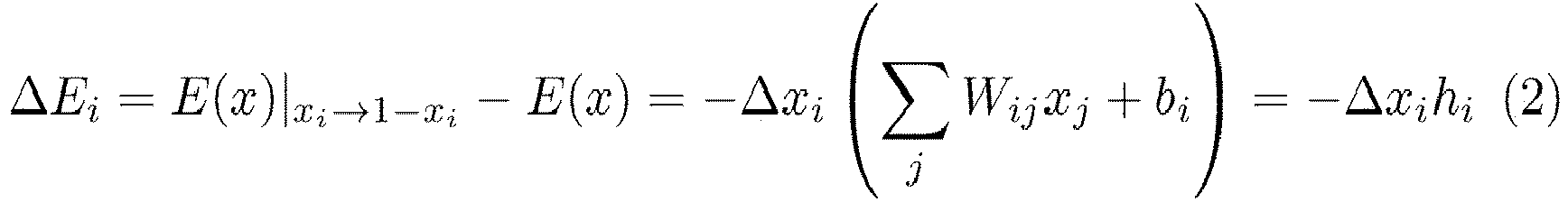
- hi is referred to as local field (LF). The amount of change in hi responsive to a change in the value of xj is expressed as: Δhi (j) = WijΔxj.
- In the solution search, a Metropolis or Gibbs method is used to determine whether to accept a state transition with an energy change of ΔEi, that is, a change of the value of the state variable xi. Specifically, in a neighbor search that searches for a transition from a current state to a different state with an energy lower than that of the current state, not only a transition to a state with lower energy but also a transition to a state with higher energy is stochastically accepted. For example, an acceptance probability Ai of accepting a change in the value of the state variable that causes ΔEi, is defined by equation (3) below.

- β is the reciprocal (β = 1/T) of T (T > 0), which is a parameter representing temperature, and is called inverse temperature. β and T are also referred to as temperature values hereinafter. The min operator returns the minimum value of its arguments. The upper part and lower part on the right side of equation (3) correspond to the Metropolis method and the Gibbs method, respectively.
- However, in order to search all the neighbors, n × n Wij's are used for the calculation of ΔE1 to ΔEn. As the problem size increases, there may be a case where all the Wij's are not storable in fast but relatively small-capacity memory (e.g., on-chip memory). In this case, the Wij's are stored in memory with relatively large capacity (e.g., dynamic random-access memory (DRAM)). However, the access time of a DRAM is, for example, about two orders of magnitude greater than that of an on-chip random access memory (RAM), which therefore greatly limits the processing speed.
- In view of this problem, the
data processor 10 of the present embodiment performs neighbor searches using multiple state variable groups obtained by dividing the n state variables. Each of the multiple state variable groups is hereinafter referred to as a partial neighbor. - The
data processor 10 includes afirst storing unit 11, asecond storing unit 12, a searchingunit 13, and aprocessing unit 14. - The
first storing unit 11 stores therein the values of multiple weight coefficients included in an evaluation function, which is obtained by transforming a combinatorial optimization problem. In the example ofFIG. 1 , thefirst storing unit 11 stores multiple weight coefficients divided into weight coefficient groups, each of which is associated with one of the multiple partial neighbors. - The
first storing unit 11 is, for example, a storage device which is slower but has a larger capacity than thesecond storing unit 12 to be described later. Examples of such a storage device include a volatile electronic circuit, such as a DRAM, and a non-volatile electronic circuit, such as a hard disk drive (HDD) and flash memory. - The multiple partial neighbors are generated in such a manner that the weight coefficient group associated with each partial neighbor may be stored in the
second storing unit 12. The multiple partial neighbors may be generated by theprocessing unit 14 of thedata processor 10 based on problem information (including indices of the n state variables and the n × n Wij's) stored in thefirst storing unit 11 or a different storage device. Alternatively, a device external to thedata processor 10 may generate the multiple partial neighbors. - The multiple partial neighbors are generated to satisfy, for example, the following constraints: (1) each partial neighbor represents a part (subset) of state space represented by the values of xi to xn; (2) each partial neighbor is part of the whole neighbor; (3) if state Y is a partial neighbor of state X, then state X is also a partial neighbor of state Y; and (4) the probability of transition within a partial neighbor is proportional to that within the whole neighbor, and the probability of transition out of the partial neighbor is zero. The transition probability is given by the product of a proposal probability and the acceptance probability Ai of equation (3). The proposal probability is denoted by Q(X, Y) when the state transitions from state X to state Y. Assume in an example of the present embodiment that the number of elements in a partial neighbor is m, and state transitions within the partial neighbor take place uniformly and randomly. In this case, the proposal probability is defined as: Q(X, Y) = 1/m.
- Note that the constraint (3) could read that state X is a partial neighbor of state Y even if state Y is obtained from state X via multiple state transitions to partial neighbors.
- To satisfy the above constraints, multiple partial neighbors are generated, for example, by simply dividing x1 to xn in order of indices. The multiple partial neighbors may also be generated by randomly selecting the indices and dividing x1 to xn such that each partial neighbor contains approximately the same number of state variables. Here, duplicate indices may be included in each partial neighbor. It is, however, preferable that each index be included in at least one partial neighbor. Note that, after a solution search is performed for each of the multiple partial neighbors, or after a solution search for each partial neighbor is repeated several times, indices may be randomly selected again so as to generate multiple partial neighbors and perform solution searches.
- However, the method of generating multiple partial neighbors is not limited to the method described above. For example, all combinations of two indices i and j, i.e., (1, 2), ..., (1, n), (2, 3), (2, 4), ..., (2, n), ..., and (n-1, n) may be set as a whole neighbor, which is then divided into multiple partial neighbors.
-
FIG. 1 depicts an example where n state variables are divided into I partial neighbors (N2 to N1). Taking a neighbor of one bit flipping as an example, each of N1 to NI is defined by a set of indices of state variables to be flipped. For example, N1 to NI are defined as N1 = {j1 (1), j2 (1), ..., jm (1)}, N2 = {j1 (2), j2 (2), ..., jm (2)}, ..., and NI = {j1 (I), j2 (I), ..., jm (I)}. ji (i) represents the i-th index amongst the indices of the m state variables included in Ni. - Note that different partial neighbors may contain the same indices, as illustrated in
FIG. 1 . That is, the ranges of indices included may overlap between different partial neighbors. - In the case where N1 to NI are generated as described above, the
first storing unit 11 stores therein groups of weight variables (Wij's) associated with the individual partial neighbors. For example, the Wij group of N1 includes weight coefficients between, amongst the n state variables, each of the state variables included in N1 and the rest of the state variables of N1. The Wij group of N2 includes weight coefficients between, amongst the n state variables, each of the state variables included in N2 and the rest of the state variables of N2. The Wij group of NI includes weight coefficients between, amongst the n state variables, each of the state variables included in NT and the rest of the state variables of NI. - Note that the
first storing unit 11 may also store various programs, such as a program that causes thedata processor 10 to search for solutions to combinatorial optimization problems, and various data. - The
second storing unit 12 stores therein, amongst the multiple weight coefficients included in the evaluation function, a weight coefficient group associated with a partial neighbor selected from the multiple partial neighbors. Thesecond storing unit 12 is, for example, a storage device that is faster but has a smaller capacity than the above-described first storingunit 11. Examples of such a storage device include a volatile electronic circuit, such as a static random-access memory (SRAM). Thesecond storing unit 12 may include an electronic circuit, such as a register. - The searching
unit 13 performs a solution search for each partial neighbor (corresponding to the above-described sub-problem). The searchingunit 13 reads the weight coefficient group stored in thesecond storing unit 12. The searchingunit 13 then uses the read weight coefficient group to calculate a change (ΔEi) in the value of the evaluation function, made by changing the value of each state variable of the selected partial neighbor. ΔEi is given, for example, by equation (2). The value of each state variable, the local field, the energy, and the like included in equation (2) are stored in a storing unit (e.g., a storage circuit, such as a register) (not illustrated) provided in the searchingunit 13. The searchingunit 13 is able to calculate in parallel ΔEi's for the individual state variables of the selected partial neighbor. The searchingunit 13 changes the value of one state variable of the partial neighbor, based on ΔEi's for the individual state variables and a temperature value. - The searching
unit 13 performs a solution search by Rejection-Free. In Rejection-Free, one of the state variables included in the partial neighbor is selected based on the probability given by the following equation (4), which uses the acceptance probability Ai defined by equation (3), and the value of the selected state variable is changed.
- In equation (4), m is the number of state variables included in the selected state variable group.
- The selection based on the probability given by equation (4) is equivalent to selecting the state variable with an index of j defined by the following equation (5).

- When the value of a state variable is changed, the searching
unit 13 updates the local field and energy stored in a register or the like. The searchingunit 13 searches for a solution to a combinatorial optimization problem by repeating, for each partial neighbor selected by theprocessing unit 14, an update process (including updates of the local field and energy) that includes the process of calculating ΔEi and the process of changing the value of a state variable. - The searching
unit 13 described above may be implemented using an electronic circuit, such as an application specific integrated circuit (ASIC) or field programmable gate array (FPGA). Alternatively, the searchingunit 13 may be implemented through software processing in which a program is executed by a hardware processor, such as a central processing unit (CPU), graphics processing unit (GPU), or digital signal processor (DSP). - Based on ΔEi for each state variable of the selected state variable group and a temperature value, the
processing unit 14 calculates multiplicity, which is the number of iterations in which a state remains in the same state using a usual MCMC method instead of Rejection-Free. - A time series of states obtained when performing the solution search using the usual MCMC method is expressed, for example, as {Xn} = {a, b, b, b, a, a, c, c, c, c, d, d, ...}. Hereinafter, the time series of states obtained in the solution search using the usual MCMC method is referred to as original chain.
- Because state transitions may be rejected in the usual MCMC method, the same state is sometimes maintained over multiple consecutive iterations. In the case of the original chain {Xn} above, following state a, state b is maintained for three iterations, state a is maintained for two iterations, state c is maintained for four iterations, and state d is maintained for two iterations. Such a multiplicity time series of {Xn} is expressed as {Mk} = {1, 3, 2, 4, 2, ...}.
- On the other hand, Rejection-Free does not repeat the same state. Therefore, in the case where the state time series {Xn} above is obtained by the usual MCMC method, Rejection-Free produces a state time series of {Jk} = {a, b, a, c, d, ...}.
- From the above, the multiplicity may also be said to be the number of samples of the original chain per sample obtained in the solution search by Rejection-Free.
- The
processing unit 14 calculates the multiplicity (M) based on the following equation (6).
- In equation (6), square brackets represent a floor function. r is a uniform random number value between 0 and 1. Pe represents the probability of the state changing in one iteration and is called escape probability. The multiplicity M is a random variable following the geometric distribution of Pe, and a random number following the distribution is generated by equation (6). Pe is given by the following equation (7).
- When the cumulated value of the multiplicity exceeds a predetermined threshold, the
processing unit 14 causes the searchingunit 13 to perform an update process using the weight coefficient group associated with a different partial neighbor selected from the multiple partial neighbors. For example, when the cumulated value of the multiplicity exceeds the predetermined threshold, theprocessing unit 14 selects an unselected partial neighbor from the multiple partial neighbors, then reads the values of a weight coefficient group associated with the partial neighbor from thefirst storing unit 11, and stores (writes) the read values of the weight coefficient group in thesecond storing unit 12. For example, theprocessing unit 14 overwrites the original weight coefficient group values with the values of the weight coefficient group associated with the newly selected partial neighbor. - Note that, while the searching
unit 13 is performing the update process using the values of the weight coefficient group associated with one partial neighbor, theprocessing unit 14 may select another partial neighbor in advance and store, in thesecond storing unit 12, the values of the weight coefficient group associated with the selected partial neighbor (seeFIG. 8 described later). - Thus, the
processing unit 14 has the function of a controller that controls each unit of thedata processor 10. - The
processing unit 14 may be implemented using an electronic circuit, such as an ASIC or FPGA. Alternatively, theprocessing unit 14 may be implemented through software processing in which a program is executed by a hardware processor, such as a CPU, GPU, or DSP. -
FIG. 1 depicts an example of a solution search by thedata processor 10, described above. - First, the searching
unit 13 performs a solution search within the range of N1 by Rejection-Free. In the example ofFIG. 1 , state transitions start from state X0 and then take place in the order of states X1, X2, ..., and X1. - In the solution search by Rejection-Free, such a state transition occurs per iteration; however, in a solution search according to the normal MCMC method described above, the same state may be repeated due to rejections. In the example of
FIG. 1 , state X0 is repeated for three iterations, state X1 is repeated for six iterations, and state X2 is repeated for three iterations. That is, the multiplicity (M2 (1)) of state X0 is 3, the multiplicity (M2 (1)) of state X1 is 6, and the multiplicity (M3 (1)) of state X2 is 3. - The
processing unit 14 calculates the multiplicity based on the above equation (6), and also determines whether the cumulated value exceeds a predetermined threshold. In the example ofFIG. 1 , when the multiplicity of state Xl has reached 3, the cumulated value exceeds the threshold (L0). Therefore, theprocessing unit 14 selects a different partial neighbor (N2 in the example ofFIG. 1 ), then reads the values of a weight coefficient group associated with the partial neighbor (the values of Wij group of N2) from thefirst storing unit 11 and stores them in thesecond storing unit 12. - The solution search within the range of N2 using Rejection-Free starts from state Xl. The
processing unit 14 again repeats the calculation of the multiplicity and the determination of whether the cumulated value exceeds the threshold. In the example ofFIG. 1 , the multiplicity of Xl within the range of N2 is denoted by M1 (2). - As described above, in the solution search of each partial neighbor, when the cumulated value of the multiplicity exceeds the threshold, the process moves onto the solution search for the next partial neighbor. This prevents bias from being introduced into the solution search range for each partial neighbor, which in turn enables an efficient search for a solution to the combinatorial optimization problem.
- Note that the
data processor 10 may function as a sampling device. - In the usual MCMC method, the probability distribution indicating the probability of occupancy of each state in an equilibrium state is a target distribution (e.g., a Boltzmann distribution). Therefore, by outputting, as samples, states obtained in the process of repeating state transitions or values based on the obtained states, samples following the target distribution are acquired. The acquired samples are used, for example, to calculate an expected value in machine learning or the like.
- In the
data processor 10, the searchingunit 13 outputs the values of multiple state variables for each update process (i.e., for each iteration of Rejection-Free), for example, as a sample. In addition, theprocessing unit 14 outputs the multiplicity M for the values of the multiple state variables (i.e., for each state). The target distribution is obtained by weighting the sample according to the multiplicity M. Even when thedata processor 10 is made to function as a sampling device, it is possible to suppress bias in the search ranges, thus enabling accurate sampling. - Next described is a processing flow example of a data processing method performed by the
data processor 10, with reference to a flowchart. -
FIG. 2 is a flowchart illustrating a general flow of the data processing method. - First, based on problem information of a combinatorial optimization problem in question, partial neighbors are generated by the method described above (step S10). The multiple partial neighbors may be generated by the
processing unit 14 or a device external to thedata processor 10. In addition, in step S10, the values of multiple weight coefficients included in a corresponding evaluation function are stored in thefirst storing unit 11. - Next, the
processing unit 14 selects a partial neighbor to be a solution search target (step S11), and stores the values of a weight coefficient group associated with the selected partial neighbor in the second storing unit 12 (step S12). - The searching
unit 13 performs a solution search within the range of the partial neighbor, using the values of the weight coefficient group stored in the second storing unit 12 (step S13). Further, in step S13, theprocessing unit 14 calculates the multiplicity M. - The
processing unit 14 determines whether the cumulated value of the multiplicity M exceeds a predetermined threshold (L0 in the above example) (step S14). If determining that the cumulated value does not exceed the threshold, theprocessing unit 14 returns to step S13. - If determining that the cumulated value exceeds the threshold, the
processing unit 14 determines whether there is a partial neighbor yet to be selected (step S15). If determining that there is an unselected partial neighbor, theprocessing unit 14 moves to step S16. If not, theprocessing unit 14 moves to step S18. - In step S16, the
processing unit 14 selects a partial neighbor yet to be selected. Then, theprocessing unit 14 stores, in thesecond storing unit 12, the values of a weight coefficient group associated with the newly selected partial neighbor (step S17). Subsequently, theprocessing unit 14 repeats the process starting from step S13. - In step S18, the
processing unit 14 determines whether a condition for terminating the solution search is satisfied. The condition for terminating the solution search may be, for example, whether the number of iterations has reached a predetermined number. In the case of using simulated annealing, the termination condition is, for example, whether the temperature value has reached a final temperature value. If determining that the termination condition is not satisfied, theprocessing unit 14 repeats the process starting from step 511. - For example, the partial neighbor N1 depicted in
FIG. 1 is selected, and a solution search is repeated. Note that theprocessing unit 14 may repeat the process starting from step S10 instead when determining that the termination condition is not satisfied. In this case, theprocessing unit 14 may generate multiple partial neighbors using a method different from the previous one. - When determining that the termination condition is satisfied, the
processing unit 14 outputs calculation results (step S19) and terminates the processing. The calculation results are, for example, a state (the values of x1 to xn) with the lowest energy obtained, amongst energies obtained in the update processes. - Next described are further specific procedures for a partial neighbor solution search and sampling.
-
FIG. 3 is a flowchart illustrating an example of procedures for a partial neighbor solution search and sampling. - In the case where simulated annealing is used, the following processing is performed, for example, while gradually decreasing a temperature value T from a start value to an end value according to a predetermined temperature change schedule. For example, the temperature value T is reduced by multiplying the temperature value T by a value smaller than 1 for each fixed number of iterations. In the case where the inverse temperature β is used as the temperature value T, the following processing is performed while gradually increasing the temperature value T.
- In the case where replica exchange is performed, the searching
unit 13 uses multiple replica circuits each having a different temperature value. Each replica circuit searches for a solution using the same partial neighbor. Then, the following processing is performed in each of the replica circuits. Theprocessing unit 14 exchanges replicas each time a predetermined number of iterations is repeated. For example, theprocessing unit 14 randomly selects a pair of replica circuits with adjacent temperature values amongst the multiple replica circuits, and exchanges the temperature values or states between the two selected replica circuits, with an exchange probability based on their energy or temperature difference. - As illustrated in
FIG. 3 , theprocessing unit 14 first performs an initialization process (step S20). The initialization process includes setting of the following items: initial values of the energy and local field; the aforementioned threshold (L0); the total number of partial neighbors (K in the example below); a condition for terminating the solution search (an upper limit Itr of the number of iterations in the example below). When the simulated annealing method is performed, the followings are also set: the start value and the end value of T (or β); and the value by which T (or β) is multiplied for each predetermined temperature change cycle. When the replica exchange method is performed, a temperature value for each replica circuit is set. - Then, the
processing unit 14 assigns 1 to k, which is the index of a partial neighbor (step S21). This corresponds to selecting a partial neighbor with k = 1. - Next, the
processing unit 14 assigns the above threshold value L0 to a variable L (step S22). Subsequently, the searchingunit 13 calculates ΔEi for the partial neighbor with k = 1, and theprocessing unit 14 calculates the multiplicity M (step S23). In step S23, the searchingunit 13 may select a state variable whose value is to be changed by the aforementioned Rejection-Free, but does not change the value (i.e., does not update the state) yet. - The
processing unit 14 determines whether M ≤ L (step S24). The process of step S24 corresponds to that of step S14 of determining whether the cumulated value of the multiplicity M exceeds the threshold, depicted inFIG. 2 . If determining that M ≤ L, theprocessing unit 14 moves to step S25. If not, theprocessing unit 14 moves to step S27. - In step S25, the
processing unit 14 assigns L - M to L. Then, theprocessing unit 14 causes the searchingunit 13 to update the state based on ΔEi calculated in step S23 and the temperature value (step S26). The state update is done by changing the value of one state variable of the partial neighbor, selected by the aforementioned Rejection-Free. With the state update, the local field and energy are also updated. In addition, when the updated energy is the lowest ever, the searchingunit 13 may hold the value of the lowest energy and the state with the lowest energy. - Note that, in step S26, the
processing unit 14 outputs (or stores in a storing unit not illustrated) the state before the update and the multiplicity M calculated for the state before the update. - After step S26, the
processing unit 14 repeats the process starting from step S23. - In step S27, the
processing unit 14 outputs (or stores in a storing unit not illustrated) a sample (here, including the current state and L as the multiplicity of the state). No state update takes place in step S27. - After step S27, the
processing unit 14 determines whether k ≥ K (step S28). If determining that k ≥ K, theprocessing unit 14 moves to step S30. If not, theprocessing unit 14 moves to step S29. - In step S29, the
processing unit 14 assigns k + 1 to k so as to switch the solution search target to the next partial neighbor. Subsequently, theprocessing unit 14 repeats the process starting from step S22. - In step S30, the
processing unit 14 determines whether itr < Itr, where itr is a variable representing the number of iterations and has an initial value of 1. If determining that itr < Itr, theprocessing unit 14 moves to step S31. If not, theprocessing unit 14 moves to step S32. - In step S31, the
processing unit 14 assigns itr + 1 to itr. Subsequently, theprocessing unit 14 repeats the process starting from step S21. The process of step S32 is the same as that of step S19 ofFIG. 2 . - Note that the processing order illustrated in
FIGS. 2 and3 is merely an example, and the order may be changed as appropriate. - Even when the solution search is performed for each partial neighbor by Rejection-Free, the above-described processing allows for suppressing bias in the solution search range among partial neighbors, thus enabling accurate sampling.
-
FIG. 4 illustrates a circuit example for selecting a state variable whose value is to be changed by Rejection-Free. - The searching
unit 13 includes ki calculation circuits 13a1, 13a2, ..., and 13am and aselection circuit unit 13b used to select a state variable whose value is to be changed by Rejection-Free. - The ki calculation circuits 13a1 to 13am calculate max (0, ΔEi) + Tln(-ln(ri)) in the above equation (5) as ki. Then, the ki calculation circuits 13a1 to 13am output ki's and their indices (i). For example, the ki calculation circuit 13a1 outputs k1 and i = 1. The ki calculation circuit 13a2 outputs k2 and i = 2. The ki calculation circuit 13am outputs km and i = m.
- The
selection circuit unit 13b includes multiple selection circuits (selection circuits 13b1, 13b2, 13b3, 13b4, 13b5 and so on) arranged over multiple levels in a tree like structure. - Each of the multiple selection circuits outputs the smaller of the two ki's and its index. When the values of the two ki's are equal, ki with the smaller index and the index are output. The index (j) output from the selection circuit 13b5 at the lowest level is j of equation (5), which is the index of a state variable whose value is to be changed.
-
FIG. 5 illustrates an update of energy. - The searching
unit 13 includes anenergy update circuit 13c depicted inFIG. 5 . When a value of xk is changed, theenergy update circuit 13c updates the energy based on the change Δxk and hk, which is the local field of xk. Specifically, the energy E is updated by subtracting Δxkhk from the original energy E. - Next described is a configuration example of the
processing unit 14 that calculates the multiplicity M. -
FIG. 6 illustrates an example of a processing unit. - The
processing unit 14 includes an escapeprobability calculation circuit 20, amultiplicity calculation circuit 21, a uniform randomnumber generation circuit 22, and a partial neighbor switchingdetermination circuit 23. - The escape
probability calculation circuit 20 receives ΔE1, ΔE2, ..., and ΔEm output from the searchingunit 13. Then, the escapeprobability calculation circuit 20 calculates the escape probability Pe given by the above equation (7). - The
multiplicity calculation circuit 21 calculates the multiplicity M given by the above equation (6) based on Pe calculated by the escapeprobability calculation circuit 20 and a uniform random number r. - The uniform random
number generation circuit 22 generates the uniform random number r between 0 and 1. The uniform randomnumber generation circuit 22 is implemented using, for example, a Mersenne Twister, linear feedback shift register (LFSR), or the like. - The partial neighbor switching
determination circuit 23 switches a partial neighbor on which the searchingunit 13 performs a solution search when the cumulated value of the multiplicity M exceeds a threshold (L0 in the example ofFIG. 1 ). - Pe is given by the above equation (7), as described above. Further, equation (7) may be expanded as the following equation (8).

- εi in equation (8) is given by the following equation (9).

- Pe defined as equation (8) is calculated by the escape
probability calculation circuit 20 described below. -
FIG. 7 illustrates an example of the escape probability calculation circuit. - The escape
probability calculation circuit 20 includes εi calculation circuits 20a1, 20a2, ..., and 20am, Ai calculation circuits 20b1, 20b2, ..., and 20bm, anaddition circuit 20c, aregister 20d, and amultiplication circuit 20e. - Each of the εi calculation circuits 20a1 to 20am calculates εi given by equation (9) based on ΔEi and β (inverse temperature) . For example, the εi calculation circuit 20a1 calculates ε1; the εi calculation circuit 20a2 calculates ε2; and the εi calculation circuit 20am calculates εm.
- Each of the Ai calculation circuits 20b1 to 20bm calculates the acceptance probability Ai (= exp(-εi)) of accepting a change in the value of a state variable that causes an energy change of ΔEi. For example, the Ai calculation circuit 20b1 calculates exp(-ε1); the Ai calculation circuit 20b2 calculates exp(-ε2); and the Ai calculation circuit 20bm calculates exp(-εm).
- The
addition circuit 20c adds up exp(-ε1) to exp(-εm). - The
register 20d holds and outputs the addition results output from theaddition circuit 20c in synchronization with a clock signal. Theregister 20d initializes the contents held therein to 0 upon receiving a reset signal. - The
multiplication circuit 20e multiplies the value output from theregister 20d by 1/m and outputs the resulting escape probability Pe. - Note that converting the calculation of the escape probability to, for example, a base-2 operation enables fast calculation. In order to perform such calculation, εi is defined by equation (10) below.
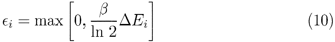
- εi given by equation (10) is a value obtained by multiplying εi of equation (9) by 1/ln2 = 1.433. When using εi of equation (10), the escape probability Pe is given by equation (11) below.

- Assuming that the escape probability Pe is calculated in the aforementioned operation, each of the εi calculation circuits 20a1 to 20am calculates εi given by equation (10) based on ΔEi and β (inverse temperature) . Then, each of the Ai calculation circuits 20b1 to 20bm calculates the value of 2 to the power of -εi. The calculation of 2^-εi may be performed by a shift operation using a shift register. This allows for faster operation compared to the case of calculating exp(-εi).
- Note that the quantization error is sufficiently small if a decimal representation with about two decimal places is used as εi.
- The
processing unit 14 may find an approximate value for the multiplicity M. For example, when a value is changed, the multiplicity M may be approximately obtained from the number of state variables satisfying -log(ri) > βΔEi (see, for example,Japanese Laid-open Patent Publication No. 2020-135727 -
FIG. 8 illustrates an example of how to switch a partial neighbor. - In the example of
FIG. 8 , thesecond storing unit 12 includes afirst storage area 12a, asecond storage area 12b, and switches 12c and 12d. - The
first storage area 12a is provided for storing a Wij group associated with a partial neighbor with, for example, an odd index. Thesecond storage area 12b is provided for storing a Wij group associated with a partial neighbor with, for example, an even index. That is, in the example ofFIG. 8 , thesecond storing unit 12 is able to store Wij groups associated with two partial neighbors at once. - Based on a switch control signal supplied from the
processing unit 14, theswitch 12c switches storage space for each Wij group read from thefirst storing unit 11 between thefirst storage area 12a and thesecond storage area 12b. - Based on a switch control signal supplied from the
processing unit 14, theswitch 12d switches the Wij group to be supplied to the searchingunit 13 between one stored in thefirst storage area 12a and one stored in thesecond storage area 12b. - When causing the searching
unit 13 to perform an update process using the Wij group stored in thefirst storage area 12a, theprocessing unit 14 connects thefirst storage area 12a and the searchingunit 13 with theswitch 12d. While the update process using the Wij group stored in thefirst storage area 12a is being performed, theprocessing unit 14 connects thefirst storing unit 11 and thesecond storage area 12b with theswitch 12c. Then, theprocessing unit 14 reads, from thefirst storing unit 11, the Wij group associated with the partial neighbor for which the solution search is performed next, and writes the read Wij group in thesecond storage area 12b. - When the solution search using the Wij group stored in the
first storage area 12a is completed, theprocessing unit 14 flips theswitch 12d and then causes the searchingunit 13 to perform an update process using the Wij group stored in thesecond storage area 12b. - According to the aforementioned configuration, it is possible to shorten the time needed to read a Wij group in switching a partial neighbor for the solution search, thus making the solution search more efficient.
- In the above description, the state variables are binary variables each taking a value of 0 or 1. However, the state variables may be continuous variables instead.
- In the case of using binary variables, a state transition is generated by flipping the value of a binary variable (adding Δxi = 1 - 2xi to the original xi). On the other hand, in the case of using continuous variables, a state transition is generated by adding or subtracting a continuous random variable Δxi to or from the original xi. Whether to add or subtract is randomly selected with a probability of 50%.
- In the solution search for a partial neighbor, the searching
unit 13 generates the random variable Δxi that follows a probability distribution (for example, a normal distribution with an average value of 0) for each real-number state variable included in the partial neighbor. - Partial neighbors are generated in the same manner as in the case of using binary variables. Note however that, in the solution search, each time a partial neighbor subject to the solution search is changed, the searching
unit 13 again generates the random variable Δxi for the new partial neighbor. - The evaluation function in the case of using continuous variables is given by the following equation (12).

- λi in equation (12) is a coefficient with a value greater than 0.
- The amount of change in the energy E obtained when the value of the state variable xi has changed to xi + δiΔxi is given by equation (13) below.

- Here, δi is a random number that is generated for each xi and takes a value of +1 or -1 with a probability of 50%. The value of Δxi is constant and does not change during the solution search for a partial neighbor. The local field (hi) of equation (13) is given by equation (14) below.

- Cij of equation (14) is given by equation (15) below.
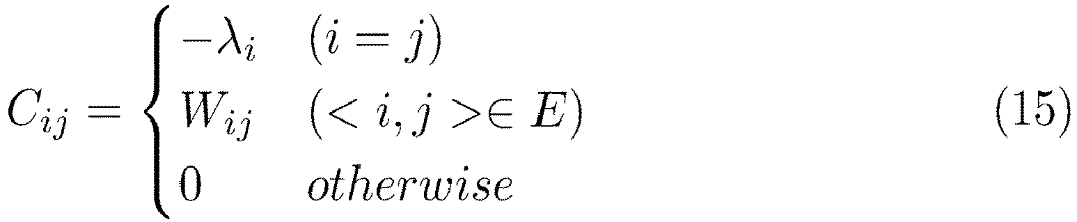
- Note that, in equation (15), a set E is a set of coefficient indices with non-zero weight coefficients wij's.
- Equations (12) and (14) are used to calculate the initial values of the energy and the local field. When a change is made to the value of a state variable, the energy and local field are updated by difference calculation as in the case of using binary variables. In addition, when the state variable xj is selected and changed to xj + δjΔxj, the value of Δxj is maintained and the value of δj is randomly generated again.
- When the value of xj changes to xj + δjΔxj, the energy E is updated by subtracting δjΔxjhj from the original energy E. The local field hi is updated by adding CijδjΔxj to the original hi. At this time, because the random number δj is generated again for the changed xj, the value of hi is updated based on the difference generated by the change in the value of δj. This update is done by subtracting λjεj/2 from the original hi. εj is the amount of change in δjΔxj and is given by equation (16) below.

- In equation (16), δj (old) is the value of δj just before changing the value of xj, and δj is the newly generated value.
- Note that, in the case of using continuous variables, the local field in response to switching of a partial neighbor subject to the solution search is updated by subtracting λiεi/2 from the original hi. εi is the amount of change in the random variable δiΔxi for the partial neighbor used and is given by equation (17) below.

- In equation (17), (δiΔxi) (old) is the value of δiΔxi for xi in the state just before the switching of the partial neighbor.
-
FIG. 9 is a flowchart illustrating an example of procedures for a partial neighbor solution search where continuous variables are used. - The procedures to be followed when using continuous variables are almost the same as in the case of using binary variables (
FIG. 3 ). Steps S40 and S41 are the same as steps S20 and S21, respectively, ofFIG. 3 . - After step S41, in the case of using continuous variables, the searching
unit 13 generates the random variable Δxi for each state variable included in the partial neighbor (step S42), as described above. Subsequent steps S43 to S53 are the same as steps S22 to S32 ofFIG. 3 . - Note however that, in order to switch the target of the solution search to the next partial neighbor, the process starting from step S42 is repeated after the process of assigning k + 1 to k (step S50). In addition, if the value of xj is changed to xj + δjΔxj, as described above, in the state update of step S47, the energy E is updated by subtracting δjΔxjhj from the original energy E. The local field hi is updated by adding CijδjΔxj to the original hi.
- As described above, the method of the present embodiment is also applicable to the case of using continuous variables for the state variables.
-
FIG. 10 illustrates a hardware example of a data processor. - The
data processor 30 is, for example, a computer, and includes aprocessor 31, aRAM 32, anHDD 33, aGPU 34, aninput device interface 35, amedia reader 36, acommunication interface 37, and anaccelerator card 38. These units are connected to a bus. - The
processor 31 functions, for example, as theprocessing unit 14 ofFIG. 1 . Theprocessor 31 is, for example, a GPU or CPU which includes an arithmetic circuit for executing program instructions and a storage circuit, such as a cache memory. Theprocessor 31 reads out at least part of programs and data stored in theHDD 33, loads them into theRAM 32, and executes the loaded programs. Note that theprocessor 31 may include two or more processor cores. In addition, thedata processor 30 may include two or more processors. The term "processor" may be used to refer to a set of processors (multiprocessor). - The
RAM 32 is volatile semiconductor memory for temporarily storing therein programs to be executed by theprocessor 31 and data to be used by theprocessor 31 for its computation. Note that thedata processor 30 may be provided with a different type of memory other than theRAM 32, or may be provided with two or more memory devices. - The
HDD 33 is a non-volatile storage device to store therein software programs, such as an operating system (OS), middleware, and application software, and various types of data. The programs include, for example, a program that causes thedata processor 30 to execute a process of searching for a solution to a combinatorial optimization problem. Note that thedata processor 30 may be provided with a different type of memory device, such as flash memory or a solid state drive (SSD), or may be provided with two or more non-volatile storage devices. - The
GPU 34 produces video images (for example, images with the calculation results of a combinatorial optimization problem) in accordance with drawing commands from theprocessor 31 and displays them on a screen of adisplay 34a coupled to thedata processor 30. Thedisplay 34a may be any type of display, such as a cathode ray tube (CRT) display; a liquid crystal display (LCD); a plasma display panel (PDP); or an organic electroluminescence (OEL) display. - The
input device interface 35 receives an input signal from aninput device 35a connected to thedata processor 30 and supplies the input signal to theprocessor 31. Various types of input devices may be used as theinput device 35a, for example, a pointing device, such as a mouse, a touch panel, a touch-pad, or a trackball; a keyboard; a remote controller; or a button switch. A plurality of types of input devices may be connected to thedata processor 30. - The
media reader 36 is a reader for reading programs and data recorded in astorage medium 36a. As thestorage medium 36a, any of the following may be used: a magnetic disk, an optical disk, a magneto-optical disk (MO), and a semiconductor memory. Examples of the magnetic disk are a flexible disk (FD) and HDD. Examples of the optical disk are a compact disc (CD) and a digital versatile disc (DVD). - The
media reader 36 copies programs and data read from thestorage medium 36a to a different storage medium, for example, theRAM 32 or theHDD 33. The read programs are executed, for example, by theprocessor 31. Note that thestorage medium 36a may be a portable storage medium, and may be used to distribute the programs and data. Thestorage medium 36a and theHDD 33 are sometimes referred to as computer-readable storage media. - The
communication interface 37 is connected to anetwork 37a and communicates with different information processors via thenetwork 37a. Thecommunication interface 37 may be a wired communication interface connected via a cable to a communication device, such as a switch, or may be a wireless communication interface connected via a wireless link to a base station. - The
accelerator card 38 is a hardware accelerator for searching for solutions to combinatorial optimization problems. Theaccelerator card 38 includes anFPGA 38a and aDRAM 38b. - The
FPGA 38a implements, for example, the functions of thesecond storing unit 12 and the searchingunit 13 ofFIG. 1 . - The
DRAM 38b implements, for example, the function of thefirst storing unit 11 ofFIG. 1 . - Note that the
FPGA 38a may implement the function of theprocessing unit 14 ofFIG. 1 . In addition, theaccelerator card 38 may be provided in plurality. - The hardware configuration for realizing the
data processor 10 ofFIG. 1 is not limited to that depicted inFIG. 10 . For example, the functions of thesecond storing unit 12, the searchingunit 13, and theprocessing unit 14 may be implemented by a processor, such as a GPU having multiple cores, and memory provided within the processor. - The processes performed by the
data processors FIGS. 2 ,3 , and9 ) may be implemented via software by causing thedata processors - Such a program may be recorded in a computer-readable storage medium. Examples of such a computer-readable storage medium include a magnetic disk, an optical disk, a magneto-optical disk, and semiconductor memory. Examples of the magnetic disk are a flexible disk (FD) and HDD. Examples of the optical disk are a compact disc (CD), CD-recordable (CD-R), CD-rewritable (CD-RW), digital versatile disc (DVD), DVD-R, and DVD-RW. The program may be recorded on portable storage media and then distributed. In such a case, the program may be executed after being copied from such a portable storage medium to a different storage medium.
- Having described aspects of the data processor, program, and data processing method based on the embodiment above, they are merely examples and the particular details of these illustrative examples shall not be construed as limitations on the appended claims.
- According to an aspect, it is possible to perform an efficient solution search.
Claims (7)
- A data processing apparatus comprising:first memory means (11) for storing values of a plurality of weight coefficients included in an evaluation function which is obtained by transforming a combinatorial optimization problem;second memory means (12) for storing, amongst the plurality of weight coefficients, values of a weight coefficient group which is associated with a state variable group selected from a plurality of state variable groups, the plurality of state variable groups being obtained by dividing a plurality of state variables included in the evaluation function;searching means (13) for searching for a solution to the combinatorial optimization problem by repeating an update process, the update process including a process of calculating, using the values of the weight coefficient group read from the second memory means, a change in a value of the evaluation function responsive to changing a value of each of state variables of the state variable group and a process of changing a value of one of the state variables of the state variable group based on the change and a temperature value; andprocessing means (14) for calculating, based on the change and the temperature value, multiplicity indicating a number of iterations in which the values of the state variables of the state variable group are maintained in searching for the solution using a Markov chain Monte Carlo method, and causing, responsive to a cumulated value of the multiplicity exceeding a predetermined threshold, the searching means to perform the update process using the values of the weight coefficient group which is associated with a different state variable group selected from the plurality of state variable groups.
- The data processing apparatus according to claim 1, wherein:the searching means outputs values of the plurality of state variables for each of the update processes, andthe processing means outputs the multiplicity for each state formed by the values of the plurality of state variables.
- The data processing apparatus according to claim 1, wherein:the processing meanscalculates, for each of the state variables of the state variable group, an acceptance probability of accepting a value change based on the change and the temperature value,calculates an escape probability by dividing a sum of the acceptance probability by a number of the state variables of the state variable group, andcalculates the multiplicity based on the escape probability and a random number value.
- The data processing apparatus according to claim 3, wherein:
the processing means calculates the acceptance probability by shift operation. - The data processing apparatus according to claim 1, wherein:the second memory means includes a first storage area (12a) and a second storage area (12b), andwhile the searching means is performing the update process using the values of the weight coefficient group stored in the first storage area, the values of the weight coefficient group associated with the different state variable group are read from the first memory means and written to the second storage area.
- A computer program that causes a computer to execute a process comprising:storing, in first memory means (11), values of a plurality of weight coefficients included in an evaluation function which is obtained by transforming a combinatorial optimization problem;storing, in second memory means (12), amongst the plurality of weight coefficients, values of a weight coefficient group which is associated with a state variable group selected from a plurality of state variable groups, the plurality of state variable groups being obtained by dividing a plurality of state variables included in the evaluation function;searching for a solution to the combinatorial optimization problem by repeating an update process, the update process including a process of calculating, using the values of the weight coefficient group read from the second memory means, a change in a value of the evaluation function responsive to changing a value of each of state variables of the state variable group and a process of changing a value of one of the state variables of the state variable group based on the change and a temperature value;calculating, based on the change and the temperature value, multiplicity indicating a number of iterations in which the values of the state variables of the state variable group are maintained in searching for the solution using a Markov chain Monte Carlo method; andperforming, responsive to a cumulated value of the multiplicity exceeding a predetermined threshold, the update process using the values of the weight coefficient group which is associated with a different state variable group selected from the plurality of state variable groups.
- A data processing method comprising:storing, by first memory means (11), values of a plurality of weight coefficients included in an evaluation function which is obtained by transforming a combinatorial optimization problem;storing, by second memory means (12), amongst the plurality of weight coefficients, values of a weight coefficient group which is associated with a state variable group selected from a plurality of state variable groups, the plurality of state variable groups being obtained by dividing a plurality of state variables included in the evaluation function;searching, by searching means (13), for a solution to the combinatorial optimization problem by repeating an update process, the update process including a process of calculating, using the values of the weight coefficient group read from the second memory means, a change in a value of the evaluation function responsive to changing a value of each of state variables of the state variable group and a process of changing a value of one of the state variables of the state variable group based on the change and a temperature value;calculating, by processing means (14), based on the change and the temperature value, multiplicity indicating a number of iterations in which the values of the state variables of the state variable group are maintained in searching for the solution using a Markov chain Monte Carlo method, and causing, responsive to a cumulated value of the multiplicity exceeding a predetermined threshold, the searching means to perform the update process using the values of the weight coefficient group which is associated with a different state variable group selected from the plurality of state variable groups.
Applications Claiming Priority (1)
| Application Number | Priority Date | Filing Date | Title |
|---|---|---|---|
| JP2022155524A JP2024049202A (en) | 2022-09-28 | 2022-09-28 | Data processing device, program and data processing method |
Publications (1)
| Publication Number | Publication Date |
|---|---|
| EP4345696A1 true EP4345696A1 (en) | 2024-04-03 |
Family
ID=87929228
Family Applications (1)
| Application Number | Title | Priority Date | Filing Date |
|---|---|---|---|
| EP23194811.8A Pending EP4345696A1 (en) | 2022-09-28 | 2023-09-01 | Data processing apparatus, program, and data processing method |
Country Status (4)
| Country | Link |
|---|---|
| US (1) | US20240111833A1 (en) |
| EP (1) | EP4345696A1 (en) |
| JP (1) | JP2024049202A (en) |
| CN (1) | CN117786275A (en) |
Citations (3)
| Publication number | Priority date | Publication date | Assignee | Title |
|---|---|---|---|---|
| JP2020135727A (en) | 2019-02-25 | 2020-08-31 | 富士通株式会社 | Sampling device and sampling device control method |
| US20210303754A1 (en) * | 2020-03-26 | 2021-09-30 | Fujitsu Limited | Optimization apparatus and optimization method |
| US20210319154A1 (en) * | 2020-04-13 | 2021-10-14 | Fujitsu Limited | Sampling device, sampling method, and non-transitory computer-readable storage medium for storing sampling program |
-
2022
- 2022-09-28 JP JP2022155524A patent/JP2024049202A/en active Pending
-
2023
- 2023-09-01 EP EP23194811.8A patent/EP4345696A1/en active Pending
- 2023-09-11 CN CN202311168582.XA patent/CN117786275A/en active Pending
- 2023-09-25 US US18/372,413 patent/US20240111833A1/en active Pending
Patent Citations (3)
| Publication number | Priority date | Publication date | Assignee | Title |
|---|---|---|---|---|
| JP2020135727A (en) | 2019-02-25 | 2020-08-31 | 富士通株式会社 | Sampling device and sampling device control method |
| US20210303754A1 (en) * | 2020-03-26 | 2021-09-30 | Fujitsu Limited | Optimization apparatus and optimization method |
| US20210319154A1 (en) * | 2020-04-13 | 2021-10-14 | Fujitsu Limited | Sampling device, sampling method, and non-transitory computer-readable storage medium for storing sampling program |
Non-Patent Citations (5)
| Title |
|---|
| J. S. ROSENTHAL ET AL.: "Jump Markov Chains and Rejection-Free Metropolis Algorithms", COMPUTATIONAL STATISTICS, vol. 36, no. 4, 2021, pages 2789 - 2811, XP037622638, DOI: 10.1007/s00180-021-01095-2 |
| ROSENTHAL JEFFREY S ET AL: "Jump Markov chains and rejection-free Metropolis algorithms", COMPUTATIONAL STATISTICS, PHYSICA VERLAG, DE, vol. 36, no. 4, 13 March 2021 (2021-03-13), pages 2789 - 2811, XP037622638, ISSN: 0943-4062, [retrieved on 20210313], DOI: 10.1007/S00180-021-01095-2 * |
| SIGENG CHEN ET AL.: "Optimization via Rejection-Free Partial Neighbor Search", ARXIV:2205.02083, 15 April 2022 (2022-04-15) |
| SIGENG CHEN ET AL: "Optimization via Rejection-Free Partial Neighbor Search", ARXIV.ORG, CORNELL UNIVERSITY LIBRARY, 201 OLIN LIBRARY CORNELL UNIVERSITY ITHACA, NY 14853, 15 April 2022 (2022-04-15), XP091211440 * |
| SIGENG CHEN ET AL: "Sampling via Rejection-Free Partial Neighbor Search", ARXIV.ORG, CORNELL UNIVERSITY LIBRARY, 201 OLIN LIBRARY CORNELL UNIVERSITY ITHACA, NY 14853, 19 October 2022 (2022-10-19), XP091348173 * |
Also Published As
| Publication number | Publication date |
|---|---|
| JP2024049202A (en) | 2024-04-09 |
| CN117786275A (en) | 2024-03-29 |
| US20240111833A1 (en) | 2024-04-04 |
Similar Documents
| Publication | Publication Date | Title |
|---|---|---|
| EP3779616B1 (en) | Optimization device and control method of optimization device | |
| US11599073B2 (en) | Optimization apparatus and control method for optimization apparatus using ising models | |
| US11182157B2 (en) | Information processing device, arithmetic device, and information processing method | |
| US11468287B2 (en) | Information processing system, information processing apparatus, and information processing method | |
| US11199884B2 (en) | Optimization device and method of controlling optimization device utilizing a spin bit | |
| EP3896622A1 (en) | Sampling device, sampling method, and sampling program | |
| EP3937090A1 (en) | Information processing system, information processing method, and program | |
| JP7769279B2 (en) | Program, information processing method and information processing device | |
| JP7181454B2 (en) | Optimization device, optimization device control method, and optimization device control program | |
| EP4345696A1 (en) | Data processing apparatus, program, and data processing method | |
| US20250005406A1 (en) | Data processing device, computer-readable recording medium storing program, and data processing method | |
| EP4254271A1 (en) | Data processing apparatus, program, and data processing method | |
| JP7628866B2 (en) | Information processing system, information processing method, and information processing program | |
| EP4254274A1 (en) | Information processing apparatus, information processing method, and computer program | |
| JP7755157B2 (en) | Program, data processing device and data processing method | |
| EP4383137A1 (en) | Data processing device, data processing program, and data processing method | |
| JP7835978B2 (en) | Information processing device, information processing method, and program | |
| EP4131084A1 (en) | Program, data processing method, and data processing apparatus | |
| EP4645171A1 (en) | Program and data processing apparatus | |
| EP4528554A1 (en) | Computer-readable recording medium storing program, data processing device, and data processing method | |
| US20250131060A1 (en) | Computer-readable recording medium storing program, data processing device, and data processing method | |
| US20260017336A1 (en) | Data processing apparatus and data processing method | |
| EP4099227A1 (en) | Data processing apparatus, data processing method, and program | |
| JP2025001157A (en) | Program, data processing method and data processing device | |
| JP2024077351A (en) | Data processing device, program and data processing method |
Legal Events
| Date | Code | Title | Description |
|---|---|---|---|
| PUAI | Public reference made under article 153(3) epc to a published international application that has entered the european phase |
Free format text: ORIGINAL CODE: 0009012 |
|
| STAA | Information on the status of an ep patent application or granted ep patent |
Free format text: STATUS: THE APPLICATION HAS BEEN PUBLISHED |
|
| AK | Designated contracting states |
Kind code of ref document: A1 Designated state(s): AL AT BE BG CH CY CZ DE DK EE ES FI FR GB GR HR HU IE IS IT LI LT LU LV MC ME MK MT NL NO PL PT RO RS SE SI SK SM TR |
|
| STAA | Information on the status of an ep patent application or granted ep patent |
Free format text: STATUS: REQUEST FOR EXAMINATION WAS MADE |
|
| 17P | Request for examination filed |
Effective date: 20240821 |
|
| RBV | Designated contracting states (corrected) |
Designated state(s): AL AT BE BG CH CY CZ DE DK EE ES FI FR GB GR HR HU IE IS IT LI LT LU LV MC ME MK MT NL NO PL PT RO RS SE SI SK SM TR |
|
| STAA | Information on the status of an ep patent application or granted ep patent |
Free format text: STATUS: EXAMINATION IS IN PROGRESS |
|
| 17Q | First examination report despatched |
Effective date: 20250903 |