EP4312183B1 - Deep neural network based method for electromagnetic source image reconstruction - Google Patents
Deep neural network based method for electromagnetic source image reconstruction Download PDFInfo
- Publication number
- EP4312183B1 EP4312183B1 EP22187009.0A EP22187009A EP4312183B1 EP 4312183 B1 EP4312183 B1 EP 4312183B1 EP 22187009 A EP22187009 A EP 22187009A EP 4312183 B1 EP4312183 B1 EP 4312183B1
- Authority
- EP
- European Patent Office
- Prior art keywords
- electromagnetic
- neural network
- electromagnetic signal
- loss function
- implemented method
- Prior art date
- Legal status (The legal status is an assumption and is not a legal conclusion. Google has not performed a legal analysis and makes no representation as to the accuracy of the status listed.)
- Active
Links
Images

Classifications
-
- G—PHYSICS
- G01—MEASURING; TESTING
- G01R—MEASURING ELECTRIC VARIABLES; MEASURING MAGNETIC VARIABLES
- G01R33/00—Arrangements or instruments for measuring magnetic variables
- G01R33/02—Measuring direction or magnitude of magnetic fields or magnetic flux
- G01R33/10—Plotting field distribution ; Measuring field distribution
-
- G—PHYSICS
- G06—COMPUTING OR CALCULATING; COUNTING
- G06T—IMAGE DATA PROCESSING OR GENERATION, IN GENERAL
- G06T5/00—Image enhancement or restoration
- G06T5/60—Image enhancement or restoration using machine learning, e.g. neural networks
-
- G—PHYSICS
- G06—COMPUTING OR CALCULATING; COUNTING
- G06T—IMAGE DATA PROCESSING OR GENERATION, IN GENERAL
- G06T2207/00—Indexing scheme for image analysis or image enhancement
- G06T2207/20—Special algorithmic details
- G06T2207/20081—Training; Learning
-
- G—PHYSICS
- G06—COMPUTING OR CALCULATING; COUNTING
- G06T—IMAGE DATA PROCESSING OR GENERATION, IN GENERAL
- G06T2207/00—Indexing scheme for image analysis or image enhancement
- G06T2207/20—Special algorithmic details
- G06T2207/20084—Artificial neural networks [ANN]
Definitions
- the present invention concerns a computer-implemented method for reconstructing a digital image of an electromagnetic source, and a system for reconstructing a digital image of an electromagnetic source from electromagnetic imaging data.
- Predicting measurement outcomes from an underlying structure often follows directly from fundamental physical principles.
- a fundamental challenge is posed when trying to solve the inverse problem of inferring the underlying source-configuration based on measurement data.
- a key difficulty arises from the fact that such reconstructions often involve ill-posed transformations and that they are prone to numerical artefacts.
- neuronal current sources generate magnetic fields outside the body that is detected in MEG (brain imaging) or MCG (heart imaging).
- MEG neural imaging
- MCG magnetic corthelial CG
- the clinician or neuro researcher is interested in which patches of cortex get activated either during rest or in response to specific stimulus.
- determining the strength, location, and spatial extent of the sources from magnetic field data is an ill-posed problem as there is an infinite set of sources that can give rise to any given magnetic field distribution.
- the state of the art for solving this type of problems is as follows: first assume a particular parametric form of the sources (current dipoles, a multipole expansion, etc.) as well as a model for the sources and its conductivity. Then, depending on the model chosen there are then either analytical or numerical formulas relating a given source distribution to a magnetic field map outside the source.
- the first class consists in parametric modelling which assumes a small and fixed number of sources whose location and orientation may vary. The problem can be solved using either non-linear least squares search or so-called beamforming approaches.
- the second class consists in imaging approaches: the entire sample surface is tesselated into around 100k positions and a source of fixed orientation is placed at each vertex. The problem is reduced to determining set of amplitudes that best fit the data. This problem is linear, however the system of equations is highly underdetermined, and some kind of prior knowledge or constraint is required to obtain a solution. These constrains are usually formulated in a Bayesian framework.
- Deep neural networks are characterized as universal approximators having the potential to compute any non-linear function. Thus, they are good candidates in tackling reconstruction problems. While deep learning is the state of the art tool for solving many tasks in natural language processing or computer vision, serious improvements are needed to completely surpass traditional methods for reconstruction tasks. The main issue is that the knowledge provided to the model to learn is constrained to the training data set.
- the number of parameters (e.g., magnetization direction, magnetometer standoff, and magnetometer direction) influencing the reconstructed electromagnetic source image is high.
- it requires a large data set to train the network with every possible combination of control parameters.
- the network is likely to encounter measurements not seen in the training data as well as the presence of unseen noise. This is particularly problematic as even tiny perturbations in the input can produce artefacts in the reconstructed output.
- Another challenge for deep learning is that the solution is based on a "black-box" which leaves out any explanations of the reconstruction process. The estimations on new samples are statistical inferences based on previous learning without warranty on the new output.
- Pantazis et al. "MEG Source Localization via Deep Learning", ARXIV.ORG, Georgia University Library, 201 OLIN Library Georgia University Ithaca, NY 14853, December 2020 describes a deep learning solution to the problem of localization of magnetoencephalography (MEG) brain signals.
- the proposed deep model architectures are tuned for single and multiple time point MEG data, and can estimate varying numbers of dipole sources using a loss function that measures the misfit between the algorithm output and the training data label.
- Francavilla et al. describes acquiring MR signals associated with the sample from a measurement device.
- a predetermined set of coil magnetic field basis vectors associated with a surface surrounding a sample is accessed.
- a non-linear optimization problem for MR information associated with the sample and coefficients in representation of coil sensitivities is solved based on a forward model that uses the MR information as inputs and simulates response physics of the sample to output computed MR signals corresponding to the MR signals, the coefficients and the predetermined vector.
- DST-CedNet Electromagnetic source imaging
- DST-CedNet recasts ESI as a machine learning problem, where discriminative learning and latent-space representations are integrated in a convolutional encoder-decoder network (CedNet) to learn a robust mapping from the measured electroencephalography/ magnetoencephalography (EEG/MEG) signals to the brain activity.
- CedNet convolutional encoder-decoder network
- EEG/MEG electroencephalography/ magnetoencephalography
- An aim of the present invention is therefore to provide a method for reconstructing images of electromagnetic sources using neural networks which can be efficient without large training datasets.
- Another aim of the invention to provide a method for reconstructing images of electromagnetic sources using neural networks which can be efficient with less prior knowledge of the electromagnetic source.
- the present invention therefore propose to use a self-learning neural network to calculate the distribution and positions of electromagnetic sources. Rather than learning a mapping from an electromagnetic field to the electromagnetic sources based on a library of training data we propose to determine the weights and biases in the neural network 'on the fly' for each set of scan-data by repeatedly comparing the measured electromagnetic field map to the calculated electromagnetic field map, corresponding to an estimated source distribution. The difference between the measured electromagnetic map and the calculated electromagnetic map is used to iteratively train the network. This approach works no matter what forward model is used to calculate the electromagnetic map.
- the electromagnetic signal (31) may represent a physical quantity chosen among: a magnetic field, an electrical field, the gradient of a magnetic field or the gradient of an electrical field.
- the estimated electromagnetic source vector (21) may be determined using at least one of the parameters among: a value of an electromagnetic field, a first angle, a second angle, a first sensor angle, a second sensor angle, and a standoff distance between a sample and a sensor.
- the neural network (20) may be a convolutional neural network, preferentially a convolutional neural network following a U-net architecture.
- the neural network (20) may comprise at least one fully connected sub-network for estimating the first angle, the second angle, the first sensor angle and/or the second sensor.
- the neural network (20) may be a fully connected neural network.
- the computer-implemented method may further comprise a step of denoising the electromagnetic signal (11) executed prior to the step of providing the electromagnetic signal as input into the neural network.
- the stop criterion is based on a threshold loss function value and/or on a signal to noise ratio metric.
- a system for reconstructing a digital image of an electromagnetic source from electromagnetic imaging data comprising:
- the at least one electromagnetic sensor (12) may comprise one or more of the following sensors: a scanning NV magnetometer, a widefield NV magnetometer, a superconducting quantum interference device, a hallbar, a magnetic resonance force microscope, and a tomographic sensor.
- the present invention concerns a computer-implemented method for reconstructing a digital image of an electromagnetic source based on a measure of an electromagnetic signal.
- an electromagnetic source means any physical object emitting an electromagnetic field.
- the electromagnetic signal can correspond to a measure of the generated electromagnetic field or to a quantity depending on the electromagnetic field. If the source is a magnetic source generating a magnetic field B, the electromagnetic signal can be the magnetic field B, but it can also be for example the gradient VB of the magnetic field or other quantities related to the magnetic field. Similarly, if the source is an electrical source generating an electrical field E, the electromagnetic signal can be the electrical field E, but also the gradient VE of the electrical field.
- the aim of the present method is to input the electromagnetic signal into a neural network which will output an estimation of a magnetization vector or of a polarization vector. Based on this estimation, an estimation of the electromagnetic signal is determined using the linear relation between either the magnetic field and the magnetization vector, or between the electrical field and the electric polarization vector. Finally a loss function depending on the electromagnetic signal and the estimated electromagnetic signal is determined and minimized to find an optimal estimated electromagnetic source vector which can be used to reconstruct the digital image of the electromagnetic source. This can for example serve to reconstruct magnetization maps of magnetic source or current density maps.
- the term "vector” may refer to a unique vector or it may refer to a "vector field".
- the present method allows the reconstruction of an estimated electromagnetic source vector, which can be for example represent a magnetic field which is a vector field.
- the estimated electromagnetic source vector could be understood as a unique vector of a vector field, or as the vector field itself.
- the meaning of the term “vector” shall be clear for the person skilled in the art depending from the context in which it is used.
- the electromagnetic source is a magnetic source generating a magnetic field B
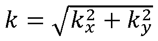
- the relation between the signal and the source is best expressed in the Fourier space.
- the magnetization vector M M ( x, y ) is confined to a two-dimensional plane ( x, y ) and that the stray field B is measured in a parallel plane at an approximately known height z', i.e.
- the transformation from a magnetisation map to a magnetic field map is therefore a well-posed forward transformation with a unique solution.
- the inverse problem of transforming from a magnetic field map to a magnetization map is ill-posed as the transformation matrix A is singular (its determinant is equal to zero), such that there is an infinite number of solutions for M ⁇ .
- the electromagnetic source is an electrical source
- the electromagnetic signal represents the electrical field E .
- the goal of the invention is to develop a neural network parametrized by a set of parameters ⁇ that will learn to operate as the inverse of the transformation matrix A -1 .
- Fig. 1 illustrates a typical operation of the method of the present invention.
- the first step of the present computer-implemented method consists in receiving an an electromagnetic signal 11 acquired by an electromagnetic sensor sensing said electromagnetic source. This may signify that a computer receives the electromagnetic signal from a sensor in real time or that the electromagnetic signal has been stored on a storing device and has been later received by a computer.
- the electromagnetic signal 11 is provided as input into a neural network 20 parametrized by a set of trainable parameters ⁇ .
- the neural network outputs an estimated electromagnetic source vector 21 associated with the electromagnetic signal 11.
- the estimated electromagnetic source vector 21 can be seen as an approximation of the target result which is a digital image 50 of the electromagnetic source 10.
- the estimated electromagnetic signal obtained in the second step can therefore be seen as an approximation of the magnetization vector M ⁇ parametrized by the set of parameters ⁇ .
- the third step of the present method consists in determining a suitable loss function 30 to be able to train the neural network 20. This is a key step as it is the choice of the loss function 30 that allows the neural network 20 to be efficient without needing large training datasets.
- the loss function 30 is determined by performing the well-posed forward transformation on the neural network output, i.e. on the estimated electromagnetic source vector 21, to transform it into an estimated electromagnetic signal 31. This new signal can therefore be seen as an approximation of the electromagnetic signal 11 based on the estimated electromagnetic source vector 21.
- the loss function 30 depends on both the electromagnetic signal 11 and the estimated electromagnetic signal 31. More precisely, the loss function 30 is designed to quantify the difference between the measured electromagnetic signal and the estimated electromagnetic signal. This difference can be quantified in various different ways using traditional norms such as L 1 or L 2 norms. Any type of norm may be used without departing from of scope of the invention as the key point here is the dependency of the loss function on the electromagnetic signal and the estimated electromagnetic signal.
- This choice of this family of loss functions 30 allows the neural network 20 to be efficient without prior training on large datasets with ground truth values.
- a loss function only depends on the original electromagnetic signal 11 and on the estimated electromagnetic signal 31. That allows a model to train without the required ground-truth value. Moreover, it can directly learn on a single new input without previous training. So instead of traditionally training on a dataset and using the learned parameters to make new predictions, a network updates its parameters ⁇ directly on the measured quantity which is the electromagnetic signal. The output of the network is not a statistical inference anymore but a solution depending on the well-posed forward transformation. Thus, the model's knowledge is not limited to a previous dataset but is directly taken from the input. Seeing that the loss function depends on the well-posed forward transformation, the proposed solution is ensured to be physically relevant. To this extent, the neural network is efficient while being untrained.
- this method fundamentally changes the ability to quantitatively determine from a stray-magnetic field image the magnetization of magnetic materials and current distributions in semiconductors, metals, or biological tissue. These capabilities are of scientific value, but even more so in the semiconductor industry (for the inspection of integrated circuits) or the magnetic memory industry for failure analysis and device development.
- is a norm.
- the term C p only depends on the input electromagnetic signal S and on the estimated electromagnetic signal S ⁇ . In particular, there is no dependence on any ground-truth value of the target electromagnetic source digital image.
- the norm ⁇ ⁇ ⁇ can be any norm commonly used in machine learning or more generally, any norm matching the dimensions of its argument.
- the absolute mean norm L 1 or the Euclidean norm L 2 are good candidates, however, many other norms may serve to the purpose of the invention.
- This loss function 30 can be seen as a regularization term.
- regularization acts on the parameters ⁇ size in order to overcome overfitting.
- a physics regularization deals with the implementation of knowledge into the model. This added knowledge constraints the learning to a desired physical solution by adding a penalty term C p to a standard loss function C .
- this term is the forward solution for reconstructing the estimated electromagnetic signal from the estimated electromagnetic source vector.
- the estimated electromagnetic signal is computed from the current estimated electromagnetic source vector. By doing so, it can be compared with the original electromagnetic signal at each iteration and be included in the loss function.
- this loss function C r can be seen as a standard loss function C to which a regularization term C p has been added, for example to constraint the learning to a physically relevant solution.
- a loss function including both a standard loss function C depending on ground-truth values and on a loss function C p depending only on the input signal, can be trained by combining the traditional approach (based on the ground-truth values) using the dataset, with the feed-forward approach (based on each input electromagnetic signal).
- the electromagnetic signal 11 may represent a physical quantity selected among: a magnetic field, an electrical field, the gradient of a magnetic field or the gradient of an electrical field.
- the neural network 20 still outputs an estimated electromagnetic source vector 21 that represents an estimated magnetization or electric polarization vector. Based on this, the estimated electromagnetic signal 31 can be reconstructed by applying the relevant forward transformation and taking the gradient of the result. The loss function 30 can then be determined based on the original (measured) gradient, i.e. the electromagnetic signal, and the estimated gradient, i.e. the estimated electromagnetic signal.
- the estimated electromagnetic source vector 21 can be determined using at least one of the parameters among: a value of an electromagnetic field, a first angle, a second angle, a first sensor angle, a second sensor angle, and a standoff distance between a sample and a sensor.
- the parameters are the following: a value of a magnetic field, a first magnetization angle, a second magnetization angle, a first sensor angle, a second sensor angle and a standoff distance between a sample source and a sensor.
- the sensor is typically a magnetometer.
- the parameters are the following: a value of an electrical field, a first electric polarization angle, a second electric polarization angle, a first sensor angle, a second sensor angle, and a standoff distance between a sample and a sensor.
- the sensor is typically an electrometer.
- a border is added to the input image to match the correct format.
- a region of interest layer can be inserted to focus the learning of the network to the desired region.
- Some of the parameters listed above i.e. an electromagnetic field value, the first and second angle, the first and second sensor angle and the standoff distance between the sensor and the sample
- the two pairs of angles can be deduced by the neural network.
- a branch of the neural network can be dedicated to each of these parameters that can be deduced by the model.
- a fully-connected sub-network can therefore be dedicated to the learning of each one of these parameters.
- the neural network is itself a fully-connected network.
- noise in the original data can be amplified during the reconstruction process.
- data with excessive noise is often ruled as ineligible for reconstruction, requiring either additional measurement time or a new measurement to be taken.
- This reconstruction is no different, in fact, the ill-posed problem is known to amplify noise.
- a trained neural network one can generalize a model to get rid of the noise in the reconstruction.
- unseen perturbations will create artefacts in the reconstruction.
- the quality of the reconstruction is directly linked to the quality of the input.
- the noise beforehand can easily improve the reconstruction quality by minimizing the noise beforehand.
- the method may comprise a step of denoising the electromagnetic signal. This step is preferably executed before providing the electromagnetic signal as input into the neural network.
- Isolating the denoising from the reconstruction is valuable, as it allows for the possibility of using noisy images without the need for additional training and facilitates double checking of the denoise process itself for loss of information.
- a trained neural network model would have to learn the denoising process, and can thus generalize incorrectly for a given data set.
- a signal to noise ratio (SNR) metric can be used as a stop criterion for the learning in order to limit the amount of noise included in the reconstruction. Typically, once the SNR has reached a minimum, the learning stops even though the loss function can still be reduced.
- SNR signal to noise ratio
- stop criteria for determining when the learning of the network has to stop can be considered.
- a threshold loss function value can be chosen before or during the learning as stop criterion.
- a number of iterations of the learning process can be set as a stop criterion.
- the present invention also concerns a system for reconstructing a digital image of an electromagnetic source from electromagnetic imaging data.
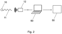
- the system comprises at least one electromagnetic sensor 12 for sensing an electromagnetic signal 11, as well as means for carrying out the computer implemented method described above to obtain a digital image 50 of the electromagnetic source 10.
- the at least one sensor can be any type of electromagnetic sensor or combinations of the like, including various types of magnetometers such as scanning NV magnetometers, widefield NV magnetometers, superconducting quantum interference devices (SQUID), hallbars, magnetic resonance force microscopes (MRFM), tomographic sensors or other imaging devices.
- magnetometers such as scanning NV magnetometers, widefield NV magnetometers, superconducting quantum interference devices (SQUID), hallbars, magnetic resonance force microscopes (MRFM), tomographic sensors or other imaging devices.
- Means for carrying out the computer-implemented method include a processing unit 60 such as a tensor processing unit (TPU), a neural network processor (NNP), an intelligence processing unit (IPU), a vision processing unit (VPU) and/or graphics processing unit (GPU). It also includes a memory unit such as SSD and/or HDD memory units or RAM memory modules.
- a processing unit 60 such as a tensor processing unit (TPU), a neural network processor (NNP), an intelligence processing unit (IPU), a vision processing unit (VPU) and/or graphics processing unit (GPU). It also includes a memory unit such as SSD and/or HDD memory units or RAM memory modules.
- the at least one sensor may be connected to the processing unit and/or memory modules. Alternatively, the signals sensed by the at least one sensor can be stored in a database that can be later accessed by the processing unit.
- acts, events, or functions of any of the algorithms described herein can be performed in a different sequence, can be added, merged, or left out altogether (for example, not all described acts or events are necessary for the practice of the methods).
- acts or events can be performed concurrently, for instance, through multi-threaded processing, interrupt processing, or multiple processors or processor cores or on other parallel architectures, rather than sequentially.
- different tasks or processes can be performed by different machines or computing systems that can function together.
- a hardware processor can include electrical circuitry or digital logic circuitry configured to process computer-executable instructions.
- a processor includes an FPGA or other programmable device that performs logic operations without processing computer-executable instructions.
- a processor can also be implemented as a combination of computing devices, e.g., a combination of a DSP and a microprocessor, a plurality of microprocessors, one or more microprocessors in conjunction with a DSP core, or any other such configuration.
- a computing environment can include any type of computer system, including, but not limited to, a computer system based on a microprocessor, a mainframe computer, a digital signal processor, a portable computing device, a device controller, or a computational engine within an appliance, to name a few.
- a software module can reside in RAM memory, flash memory, ROM memory, EPROM memory, EEPROM memory, registers, hard disk, a removable disk, a CD-ROM, or any other form of non-transitory computer-readable storage medium, media, or physical computer storage known in the art.
- An example storage medium can be coupled to the processor such that the processor can read information from, and write information to, the storage medium. In the alternative, the storage medium can be integral to the processor.
- the storage medium can be volatile or nonvolatile.
- the processor and the storage medium can reside in an ASIC.
Landscapes
- Physics & Mathematics (AREA)
- General Physics & Mathematics (AREA)
- Condensed Matter Physics & Semiconductors (AREA)
- Engineering & Computer Science (AREA)
- Theoretical Computer Science (AREA)
- Image Analysis (AREA)
Description
- The present invention concerns a computer-implemented method for reconstructing a digital image of an electromagnetic source, and a system for reconstructing a digital image of an electromagnetic source from electromagnetic imaging data.
- Predicting measurement outcomes from an underlying structure often follows directly from fundamental physical principles. However, a fundamental challenge is posed when trying to solve the inverse problem of inferring the underlying source-configuration based on measurement data. A key difficulty arises from the fact that such reconstructions often involve ill-posed transformations and that they are prone to numerical artefacts.
- This situation is well illustrated in the field of image reconstruction, and particularly by the reconstruction of current flow or magnetization maps of an electromagnetic source based on electromagnetic measurements.
- As an example, neuronal current sources generate magnetic fields outside the body that is detected in MEG (brain imaging) or MCG (heart imaging). The clinician or neuro researcher is interested in which patches of cortex get activated either during rest or in response to specific stimulus. However determining the strength, location, and spatial extent of the sources from magnetic field data is an ill-posed problem as there is an infinite set of sources that can give rise to any given magnetic field distribution.
- The state of the art for solving this type of problems is as follows: first assume a particular parametric form of the sources (current dipoles, a multipole expansion, etc.) as well as a model for the sources and its conductivity. Then, depending on the model chosen there are then either analytical or numerical formulas relating a given source distribution to a magnetic field map outside the source.
- There are two main classes of algorithms solving the inverse problem of going from a magnetic field map to a distribution of sources. The first class consists in parametric modelling which assumes a small and fixed number of sources whose location and orientation may vary. The problem can be solved using either non-linear least squares search or so-called beamforming approaches. The second class consists in imaging approaches: the entire sample surface is tesselated into around 100k positions and a source of fixed orientation is placed at each vertex. The problem is reduced to determining set of amplitudes that best fit the data. This problem is linear, however the system of equations is highly underdetermined, and some kind of prior knowledge or constraint is required to obtain a solution. These constrains are usually formulated in a Bayesian framework.
- Deep neural networks are characterized as universal approximators having the potential to compute any non-linear function. Thus, they are good candidates in tackling reconstruction problems. While deep learning is the state of the art tool for solving many tasks in natural language processing or computer vision, serious improvements are needed to completely surpass traditional methods for reconstruction tasks. The main issue is that the knowledge provided to the model to learn is constrained to the training data set.
- In the case of reconstructing an image of an electromagnetic source, the number of parameters (e.g., magnetization direction, magnetometer standoff, and magnetometer direction) influencing the reconstructed electromagnetic source image is high. Thus, it requires a large data set to train the network with every possible combination of control parameters. As such, there is a risk of training the network to only solve a subset of the total number of problems which may lead to the network converging to non-physical solutions. Moreover, the network is likely to encounter measurements not seen in the training data as well as the presence of unseen noise. This is particularly problematic as even tiny perturbations in the input can produce artefacts in the reconstructed output. Another challenge for deep learning is that the solution is based on a "black-box" which leaves out any explanations of the reconstruction process. The estimations on new samples are statistical inferences based on previous learning without warranty on the new output.
- The document EYBPOSH H. et al. "DeepCGH: 3D computer-generated holography using deep learning", Opt. Express 28, 26636-26650, 2020, discloses an algorithm for hologram synthesis that employs a convolutional neural network to perform image plane holography with unsupervised training. In order to enable the unsupervised training of the model, the algorithm computes a virtual reconstruction of the hologram based on the estimated computer-generated hologram solution and compares it to the target intensity pattern. The efficiency of this algorithm relies on the quality and quantity of the training datasets as many deep learning algorithms.
- Pantazis et al.: "MEG Source Localization via Deep Learning", ARXIV.ORG, Cornell University Library, 201 OLIN Library Cornell University Ithaca, NY 14853, December 2020 describes a deep learning solution to the problem of localization of magnetoencephalography (MEG) brain signals. The proposed deep model architectures are tuned for single and multiple time point MEG data, and can estimate varying numbers of dipole sources using a loss function that measures the misfit between the algorithm output and the training data label.
-
US 2021/311151 A1, Francavilla et al. describes acquiring MR signals associated with the sample from a measurement device. A predetermined set of coil magnetic field basis vectors associated with a surface surrounding a sample is accessed. A non-linear optimization problem for MR information associated with the sample and coefficients in representation of coil sensitivities is solved based on a forward model that uses the MR information as inputs and simulates response physics of the sample to output computed MR signals corresponding to the MR signals, the coefficients and the predetermined vector. - Wu et al.: "Research on image reconstruction algorithms based on autoencoder neural network of Restricted Boltzmann Machine (RBM)", Flow Measurement and Instrumentation, Butterworth-Heinemann, Oxford, GB, vol. 80, 12 July 2021 describes an electromagnetic tomography (EMT) image reconstruction algorithm based on autoencoder neural network of Restricted Boltzmann Machine (RBM).The encoding process of the encoder is equivalent to the object field detection process in the EMT system; the decoding process of the decoder is equivalent to the image reconstruction process.
- Gexin et al.: "Electromagnetic Source Imaging via a Data-Synthesis-Based Convolutional Encoder-Decoder Network", ARXIV.ORG, Cornell University Library,201 OLIN Library Cornell University Ithaca, NY 14853, 13 July 2022 describes a data-synthesized spatio-temporally convolutional encoder-decoder network method termed DST-CedNet is proposed for Electromagnetic source imaging (ESI). DST-CedNet recasts ESI as a machine learning problem, where discriminative learning and latent-space representations are integrated in a convolutional encoder-decoder network (CedNet) to learn a robust mapping from the measured electroencephalography/ magnetoencephalography (EEG/MEG) signals to the brain activity. In particular, by incorporating prior knowledge regarding dynamical brain activities, a novel data synthesis strategy is devised to generate large-scale samples for effectively training CedNet. This stands in contrast to traditional ESI methods where the prior information is often enforced via constraints primarily aimed for mathematical convenience.
- An aim of the present invention is therefore to provide a method for reconstructing images of electromagnetic sources using neural networks which can be efficient without large training datasets.
- Another aim of the invention to provide a method for reconstructing images of electromagnetic sources using neural networks which can be efficient with less prior knowledge of the electromagnetic source.
- According to the invention, these aims are attained by the object of the attached claims, and especially by a computer implemented method of reconstructing a digital image (50) of an electromagnetic source (10) using a neural network (20) comprising the steps of
- receiving an electromagnetic signal (11) acquired by an electromagnetic sensor (12) sensing said electromagnetic source (10),
- providing the electromagnetic signal (11) as input into a neural network (20) parametrized by a set of parameters (θ) for determining an estimated electromagnetic source vector (21) associated to the electromagnetic signal,
- determining a loss function (30),
- minimizing the loss function (30) by feed-forwarding the neural network (20) until a stop criterion is met so as to obtain an optimal electromagnetic source vector (40),
- reconstructing a digital image (50) of the electromagnetic source (10) based on the optimal electromagnetic source vector (40),
characterized in that determining the loss function (30) comprises - computing an estimated electromagnetic signal (31) based on the estimated electromagnetic source vector (21), the loss function (30) depending on the estimated electromagnetic signal (31).
- The present invention therefore propose to use a self-learning neural network to calculate the distribution and positions of electromagnetic sources. Rather than learning a mapping from an electromagnetic field to the electromagnetic sources based on a library of training data we propose to determine the weights and biases in the neural network 'on the fly' for each set of scan-data by repeatedly comparing the measured electromagnetic field map to the calculated electromagnetic field map, corresponding to an estimated source distribution. The difference between the measured electromagnetic map and the calculated electromagnetic map is used to iteratively train the network. This approach works no matter what forward model is used to calculate the electromagnetic map.
- In a preferred embodiment, the loss function (30) may comprise a regularization term of the form

- The electromagnetic signal (31) may represent a physical quantity chosen among: a magnetic field, an electrical field, the gradient of a magnetic field or the gradient of an electrical field.
- The loss function (30) may further comprise a term of the form

- The estimated electromagnetic source vector (21) may be determined using at least one of the parameters among: a value of an electromagnetic field, a first angle, a second angle, a first sensor angle, a second sensor angle, and a standoff distance between a sample and a sensor.
- In a preferred embodiment, the neural network (20) may be a convolutional neural network, preferentially a convolutional neural network following a U-net architecture.
- The neural network (20) may comprise at least one fully connected sub-network for estimating the first angle, the second angle, the first sensor angle and/or the second sensor.
- The neural network (20) may be a fully connected neural network.
- The computer-implemented method may further comprise a step of denoising the electromagnetic signal (11) executed prior to the step of providing the electromagnetic signal as input into the neural network.
- The stop criterion is based on a threshold loss function value and/or on a signal to noise ratio metric.
- According to the invention those aims are also attained by a system for reconstructing a digital image of an electromagnetic source from electromagnetic imaging data comprising:
- at least one electromagnetic sensor (12) for sensing an electromagnetic signal (11),
- means for carrying out the computer implemented method described above so as to obtain a digital image (50) of the electromagnetic source (10).
- The at least one electromagnetic sensor (12) may comprise one or more of the following sensors: a scanning NV magnetometer, a widefield NV magnetometer, a superconducting quantum interference device, a hallbar, a magnetic resonance force microscope, and a tomographic sensor.
- Exemplar embodiments of the invention are disclosed in the description and illustrated by the drawings in which:
-
Fig.1 schematically illustrates a method for reconstructing a digital image of an electromagnetic source using a neural network. -
Fig.2 schematically illustrates a system of digital image reconstruction comprising at least one electromagnetic sensor and a neural network. - The present invention concerns a computer-implemented method for reconstructing a digital image of an electromagnetic source based on a measure of an electromagnetic signal.
- In the context of this disclosure, an electromagnetic source means any physical object emitting an electromagnetic field. The electromagnetic signal can correspond to a measure of the generated electromagnetic field or to a quantity depending on the electromagnetic field. If the source is a magnetic source generating a magnetic field B, the electromagnetic signal can be the magnetic field B, but it can also be for example the gradient VB of the magnetic field or other quantities related to the magnetic field. Similarly, if the source is an electrical source generating an electrical field E, the electromagnetic signal can be the electrical field E, but also the gradient VE of the electrical field.
- The aim of the present method is to input the electromagnetic signal into a neural network which will output an estimation of a magnetization vector or of a polarization vector. Based on this estimation, an estimation of the electromagnetic signal is determined using the linear relation between either the magnetic field and the magnetization vector, or between the electrical field and the electric polarization vector. Finally a loss function depending on the electromagnetic signal and the estimated electromagnetic signal is determined and minimized to find an optimal estimated electromagnetic source vector which can be used to reconstruct the digital image of the electromagnetic source. This can for example serve to reconstruct magnetization maps of magnetic source or current density maps.
- In the context of this disclosure, the term "vector" may refer to a unique vector or it may refer to a "vector field". As an example, the present method allows the reconstruction of an estimated electromagnetic source vector, which can be for example represent a magnetic field which is a vector field. In this case, the estimated electromagnetic source vector could be understood as a unique vector of a vector field, or as the vector field itself. The meaning of the term "vector" shall be clear for the person skilled in the art depending from the context in which it is used.
- In a particular embodiment, in which the electromagnetic source is a magnetic source generating a magnetic field B, the relation between the signal and the source is best expressed in the Fourier space. Under the assumptions that the magnetization vector M = M(x, y) is confined to a two-dimensional plane (x, y) and that the stray field B is measured in a parallel plane at an approximately known height z', i.e. B = B(x, y, z'), this relation reads:

- The transformation from a magnetisation map to a magnetic field map is therefore a well-posed forward transformation with a unique solution. In contrast, the inverse problem of transforming from a magnetic field map to a magnetization map is ill-posed as the transformation matrix A is singular (its determinant is equal to zero), such that there is an infinite number of solutions for M̂.
- In another embodiment, the electromagnetic source is an electrical source, and the electromagnetic signal represents the electrical field E. In this case, there are linear systems similar to the one presented above for the Fourier transform of the magnetic field and magnetization vector, relating the Fourier transforms of the electrical field E and of the electric polarization vector P.
- The goal of the invention is to develop a neural network parametrized by a set of parameters θ that will learn to operate as the inverse of the transformation matrix A -1.
-
Fig. 1 illustrates a typical operation of the method of the present invention. - The first step of the present computer-implemented method consists in receiving an an
electromagnetic signal 11 acquired by an electromagnetic sensor sensing said electromagnetic source. This may signify that a computer receives the electromagnetic signal from a sensor in real time or that the electromagnetic signal has been stored on a storing device and has been later received by a computer. - In the second step of the present method, the
electromagnetic signal 11 is provided as input into aneural network 20 parametrized by a set of trainable parameters θ. The neural network outputs an estimatedelectromagnetic source vector 21 associated with theelectromagnetic signal 11. The estimatedelectromagnetic source vector 21 can be seen as an approximation of the target result which is adigital image 50 of theelectromagnetic source 10. - In the case mentioned above in which the electromagnetic signal represents a magnetic field B, the estimated electromagnetic signal obtained in the second step can therefore be seen as an approximation of the magnetization vector Mθ parametrized by the set of parameters θ.
- The third step of the present method consists in determining a
suitable loss function 30 to be able to train theneural network 20. This is a key step as it is the choice of theloss function 30 that allows theneural network 20 to be efficient without needing large training datasets. - The
loss function 30 is determined by performing the well-posed forward transformation on the neural network output, i.e. on the estimatedelectromagnetic source vector 21, to transform it into an estimatedelectromagnetic signal 31. This new signal can therefore be seen as an approximation of theelectromagnetic signal 11 based on the estimatedelectromagnetic source vector 21. - In the embodiment in which the
electromagnetic signal 11 is the magnetic field B itself, the estimated electromagnetic signal corresponds to Sθ = AM̂θ, meaning that the transfer matrix A has been applied to the estimated magnetization vector M̂θ (up to a Fourier transformation). - The
loss function 30 depends on both theelectromagnetic signal 11 and the estimatedelectromagnetic signal 31. More precisely, theloss function 30 is designed to quantify the difference between the measured electromagnetic signal and the estimated electromagnetic signal. This difference can be quantified in various different ways using traditional norms such as L 1 or L 2 norms. Any type of norm may be used without departing from of scope of the invention as the key point here is the dependency of the loss function on the electromagnetic signal and the estimated electromagnetic signal. - This choice of this family of
loss functions 30 allows theneural network 20 to be efficient without prior training on large datasets with ground truth values. Such a loss function only depends on the originalelectromagnetic signal 11 and on the estimatedelectromagnetic signal 31. That allows a model to train without the required ground-truth value. Moreover, it can directly learn on a single new input without previous training. So instead of traditionally training on a dataset and using the learned parameters to make new predictions, a network updates its parameters θ directly on the measured quantity which is the electromagnetic signal. The output of the network is not a statistical inference anymore but a solution depending on the well-posed forward transformation. Thus, the model's knowledge is not limited to a previous dataset but is directly taken from the input. Seeing that the loss function depends on the well-posed forward transformation, the proposed solution is ensured to be physically relevant. To this extent, the neural network is efficient while being untrained. - In the illustrative case of a magnetic source, this method fundamentally changes the ability to quantitatively determine from a stray-magnetic field image the magnetization of magnetic materials and current distributions in semiconductors, metals, or biological tissue. These capabilities are of scientific value, but even more so in the semiconductor industry (for the inspection of integrated circuits) or the magnetic memory industry for failure analysis and device development.
- In a particular embodiment, the
loss function 30 comprises a term of the form:
electromagnetic signal 11, Sθ is the estimatedelectromagnetic signal 31, and || · || is a norm. As it can be seen from the above equation, the term Cp only depends on the input electromagnetic signal S and on the estimated electromagnetic signal Sθ . In particular, there is no dependence on any ground-truth value of the target electromagnetic source digital image. - The norm ∥ · ∥ can be any norm commonly used in machine learning or more generally, any norm matching the dimensions of its argument. In particular, the absolute mean norm L 1 or the Euclidean norm L 2 are good candidates, however, many other norms may serve to the purpose of the invention.
- This
loss function 30 can be seen as a regularization term. Usually, regularization acts on the parameters θ size in order to overcome overfitting. Where a physics regularization deals with the implementation of knowledge into the model. This added knowledge constraints the learning to a desired physical solution by adding a penalty term Cp to a standard loss function C. In our case, this term is the forward solution for reconstructing the estimated electromagnetic signal from the estimated electromagnetic source vector. Thus, at the end of each iteration, the estimated electromagnetic signal is computed from the current estimated electromagnetic source vector. By doing so, it can be compared with the original electromagnetic signal at each iteration and be included in the loss function. - In another embodiment, the
loss function 30 can comprise a term
electromagnetic source vector 21 and on a ground-truth digital image of anelectromagnetic source 10, and λ is a hyper-parameter controlling the influence of Cp. As explained above, this loss function Cr can be seen as a standard loss function C to which a regularization term Cp has been added, for example to constraint the learning to a physically relevant solution. - In the presence of a training dataset containing ground-truth values, a loss function including both a standard loss function C depending on ground-truth values and on a loss function Cp depending only on the input signal, can be trained by combining the traditional approach (based on the ground-truth values) using the dataset, with the feed-forward approach (based on each input electromagnetic signal).
- As mentioned above, the
electromagnetic signal 11 may represent a physical quantity selected among: a magnetic field, an electrical field, the gradient of a magnetic field or the gradient of an electrical field. - In the case in which the
electromagnetic signal 11 is a gradient of a magnetic or electrical field, theneural network 20 still outputs an estimatedelectromagnetic source vector 21 that represents an estimated magnetization or electric polarization vector. Based on this, the estimatedelectromagnetic signal 31 can be reconstructed by applying the relevant forward transformation and taking the gradient of the result. Theloss function 30 can then be determined based on the original (measured) gradient, i.e. the electromagnetic signal, and the estimated gradient, i.e. the estimated electromagnetic signal. - The estimated
electromagnetic source vector 21 can be determined using at least one of the parameters among: a value of an electromagnetic field, a first angle, a second angle, a first sensor angle, a second sensor angle, and a standoff distance between a sample and a sensor. - In an embodiment, the parameters are the following: a value of a magnetic field, a first magnetization angle, a second magnetization angle, a first sensor angle, a second sensor angle and a standoff distance between a sample source and a sensor. In this case, the sensor is typically a magnetometer.
- In another embodiment, the parameters are the following: a value of an electrical field, a first electric polarization angle, a second electric polarization angle, a first sensor angle, a second sensor angle, and a standoff distance between a sample and a sensor. In this case, the sensor is typically an electrometer.
- The possibility to train the neural network directly on a single image makes it possible to use different architecture without facing a computational problem. In this main text, we used a convolutional neural network following a U-net architecture. Where the cost function was the mean average loss between the reconstructed electromagnetic source and the original one.
- Since convolutional layer requires a fixed-size input, a border is added to the input image to match the correct format. In order to make sure this border is not taken into account into the reconstruction, a region of interest layer can be inserted to focus the learning of the network to the desired region.
- Some of the parameters listed above (i.e. an electromagnetic field value, the first and second angle, the first and second sensor angle and the standoff distance between the sensor and the sample) used to determine the estimated electromagnetic source vector, can be deduced directly by the model. In particular, the two pairs of angles can be deduced by the neural network.
- In a particular embodiment, a branch of the neural network can be dedicated to each of these parameters that can be deduced by the model. A fully-connected sub-network can therefore be dedicated to the learning of each one of these parameters.
- In another embodiment, the neural network is itself a fully-connected network.
- One issue with implementing any reconstruction method is noise in the original data can be amplified during the reconstruction process. Thus, data with excessive noise is often ruled as ineligible for reconstruction, requiring either additional measurement time or a new measurement to be taken. This reconstruction is no different, in fact, the ill-posed problem is known to amplify noise. With a trained neural network, one can generalize a model to get rid of the noise in the reconstruction. However, one still faces the risk that unseen perturbations will create artefacts in the reconstruction.
- As the untrained neural network of the present invention learns on the input directly, the quality of the reconstruction is directly linked to the quality of the input. Thus, one can easily improve the reconstruction quality by minimizing the noise beforehand.
- For this reason, the method may comprise a step of denoising the electromagnetic signal. This step is preferably executed before providing the electromagnetic signal as input into the neural network.
- Isolating the denoising from the reconstruction is valuable, as it allows for the possibility of using noisy images without the need for additional training and facilitates double checking of the denoise process itself for loss of information. In contrast, a trained neural network model would have to learn the denoising process, and can thus generalize incorrectly for a given data set.
- The longer the untrained model learns, the more noise is taken into account into the reconstruction. In an embodiment, a signal to noise ratio (SNR) metric can be used as a stop criterion for the learning in order to limit the amount of noise included in the reconstruction. Typically, once the SNR has reached a minimum, the learning stops even though the loss function can still be reduced.
- Other stop criteria for determining when the learning of the network has to stop can be considered. A threshold loss function value can be chosen before or during the learning as stop criterion. Alternatively or complementarily, a number of iterations of the learning process can be set as a stop criterion.
- The present invention also concerns a system for reconstructing a digital image of an electromagnetic source from electromagnetic imaging data. As illustrated in
Fig. 2 , the system comprises at least oneelectromagnetic sensor 12 for sensing anelectromagnetic signal 11, as well as means for carrying out the computer implemented method described above to obtain adigital image 50 of theelectromagnetic source 10. - The at least one sensor can be any type of electromagnetic sensor or combinations of the like, including various types of magnetometers such as scanning NV magnetometers, widefield NV magnetometers, superconducting quantum interference devices (SQUID), hallbars, magnetic resonance force microscopes (MRFM), tomographic sensors or other imaging devices.
- Means for carrying out the computer-implemented method include a
processing unit 60 such as a tensor processing unit (TPU), a neural network processor (NNP), an intelligence processing unit (IPU), a vision processing unit (VPU) and/or graphics processing unit (GPU). It also includes a memory unit such as SSD and/or HDD memory units or RAM memory modules. - The at least one sensor may be connected to the processing unit and/or memory modules. Alternatively, the signals sensed by the at least one sensor can be stored in a database that can be later accessed by the processing unit.
- Depending on the embodiment, certain acts, events, or functions of any of the algorithms described herein can be performed in a different sequence, can be added, merged, or left out altogether (for example, not all described acts or events are necessary for the practice of the methods). Moreover, in certain embodiments, acts or events can be performed concurrently, for instance, through multi-threaded processing, interrupt processing, or multiple processors or processor cores or on other parallel architectures, rather than sequentially. In addition, different tasks or processes can be performed by different machines or computing systems that can function together.
- The various illustrative logical blocks and modules described in connection with the embodiments disclosed herein can be implemented or performed by a machine, a microprocessor, a state machine, a digital signal processor (DSP), an application specific integrated circuit (ASIC), an FPGA, or other programmable logic device, discrete gate or transistor logic, discrete hardware components, or any combination thereof designed to perform the functions described herein. A hardware processor can include electrical circuitry or digital logic circuitry configured to process computer-executable instructions. In another embodiment, a processor includes an FPGA or other programmable device that performs logic operations without processing computer-executable instructions. A processor can also be implemented as a combination of computing devices, e.g., a combination of a DSP and a microprocessor, a plurality of microprocessors, one or more microprocessors in conjunction with a DSP core, or any other such configuration. A computing environment can include any type of computer system, including, but not limited to, a computer system based on a microprocessor, a mainframe computer, a digital signal processor, a portable computing device, a device controller, or a computational engine within an appliance, to name a few.
- The steps of a method, process, or algorithm described in connection with the embodiments disclosed herein can be embodied directly in hardware, in a software module stored in one or more memory devices and executed by one or more processors, or in a combination of the two. A software module can reside in RAM memory, flash memory, ROM memory, EPROM memory, EEPROM memory, registers, hard disk, a removable disk, a CD-ROM, or any other form of non-transitory computer-readable storage medium, media, or physical computer storage known in the art. An example storage medium can be coupled to the processor such that the processor can read information from, and write information to, the storage medium. In the alternative, the storage medium can be integral to the processor. The storage medium can be volatile or nonvolatile. The processor and the storage medium can reside in an ASIC.
- Conditional language used herein, such as, among others, "can," "might," "may," "e.g.," and the like, unless specifically stated otherwise, or otherwise understood within the context as used, is generally intended to convey that certain embodiments include, while other embodiments do not include, certain features, elements or states. Thus, such conditional language is not generally intended to imply that features, elements or states are in any way required for one or more embodiments or that one or more embodiments necessarily include logic for deciding, with or without author input or prompting, whether these features, elements or states are included or are to be performed in any particular embodiment. The terms "comprising," "including," "having," and the like are synonymous and are used inclusively, in an open-ended fashion, and do not exclude additional elements, features, acts, operations, and so forth. Also, the term "or" is used in its inclusive sense (and not in its exclusive sense) so that when used, for example, to connect a list of elements, the term "or" means one, some, or all of the elements in the list. Further, the term "each," as used herein, in addition to having its ordinary meaning, can mean any subset of a set of elements to which the term "each" is applied.
-
- 10
- Electromagnetic source
- 11
- Electromagnetic signal
- 12
- Electromagnetic sensor
- 20
- Neural network
- 21
- Estimated electromagnetic source vector
- 30
- Loss function
- 31
- Estimated electromagnetic signal
- 40
- Optimal electromagnetic source vector
- 50
- Digital image
- 60
- Computing unit
Claims (12)
- A computer implemented method of reconstructing a digital image (50) of an electromagnetic source (10) using a neural network (20) comprising the steps ofreceiving an electromagnetic signal (11) acquired by an electromagnetic sensor (12) sensing said electromagnetic source (10),providing the electromagnetic signal (11) as input into a neural network (20) parametrized by a set of parameters (θ) and obtaining as an output of the neural network (20), an estimated electromagnetic source vector (21) associated to the electromagnetic signal,determining a loss function (30),minimizing the loss function (30) by feed-forwarding the neural network (20) until a stop criterion is met so as to obtain an optimal electromagnetic source vector (40),reconstructing a digital image (50) of the electromagnetic source (10) based on the optimal electromagnetic source vector (40),
characterized in that determining the loss function (30) comprisescomputing an estimated electromagnetic signal (31) by applying a well-posed forward transformation on the estimated electromagnetic source vector (21), the loss function (30) depending on the electromagnetic signal (11) and the estimated electromagnetic signal (31). - Computer implemented method according to claim 1, wherein the loss function (30) comprises a regularization term of the form

- Computer implemented method according to the preceding claim wherein said electromagnetic signal (31) represents a physical quantity chosen among: a magnetic field, an electrical field, the gradient of a magnetic field or the gradient of an electrical field.
- Computer implemented method according to any of the claim 2 to 3, wherein the loss function (30) further comprises a term of the form

- Computer implemented method according to any of the preceding claims, wherein the estimated electromagnetic source vector (21) is determined using at least one of the parameters among: a value of an electromagnetic field, a first angle, a second angle, a first sensor angle, a second sensor angle, and a standoff distance between a sample and a sensor.
- Computer implemented method according to any of the preceding claims, wherein the neural network (20) is a convolutional neural network, preferentially a convolutional neural network following a U-net architecture.
- Computer implemented method according to claim 5, wherein the neural network (20) comprises at least one fully connected sub-network for estimating the first angle, the second angle, the first sensor angle and/or the second sensor.
- Computer implemented method according to any of the claims 1 to 4, wherein the neural network (20) is a fully connected neural network.
- Computer implemented method according to any of the preceding claims, further comprising a step of denoising the electromagnetic signal (11) prior to the step of providing the electromagnetic signal as input into the neural network.
- Computer implemented method according to any of the preceding claims, wherein said the minimizing of the loss function (30) by feed-forwarding the neural network (20) is stopped based on a stop criterion depending on a threshold loss function value and/or on a signal to noise ratio metric.
- A system for reconstructing a digital image of an electromagnetic source from electromagnetic imaging data comprising:at least one electromagnetic sensor (12) for sensing an electromagnetic signal (11),means for carrying out the computer implemented method of claims 1 to 10 so as to obtain a digital image (50) of the electromagnetic source (10).
- System according to claim 11, wherein the at least one electromagnetic sensor (12) comprises one or more of the following sensors: a scanning NV magnetometer, a widefield NV magnetometer, a superconducting quantum interference device, a hallbar, a magnetic resonance force microscope, and a tomographic sensor.
Priority Applications (2)
| Application Number | Priority Date | Filing Date | Title |
|---|---|---|---|
| EP22187009.0A EP4312183B1 (en) | 2022-07-26 | 2022-07-26 | Deep neural network based method for electromagnetic source image reconstruction |
| PCT/IB2023/057422 WO2024023665A1 (en) | 2022-07-26 | 2023-07-20 | Deep neural network based method for electromagnetic source image reconstruction |
Applications Claiming Priority (1)
| Application Number | Priority Date | Filing Date | Title |
|---|---|---|---|
| EP22187009.0A EP4312183B1 (en) | 2022-07-26 | 2022-07-26 | Deep neural network based method for electromagnetic source image reconstruction |
Publications (2)
| Publication Number | Publication Date |
|---|---|
| EP4312183A1 EP4312183A1 (en) | 2024-01-31 |
| EP4312183B1 true EP4312183B1 (en) | 2025-06-11 |
Family
ID=82939850
Family Applications (1)
| Application Number | Title | Priority Date | Filing Date |
|---|---|---|---|
| EP22187009.0A Active EP4312183B1 (en) | 2022-07-26 | 2022-07-26 | Deep neural network based method for electromagnetic source image reconstruction |
Country Status (2)
| Country | Link |
|---|---|
| EP (1) | EP4312183B1 (en) |
| WO (1) | WO2024023665A1 (en) |
Families Citing this family (2)
| Publication number | Priority date | Publication date | Assignee | Title |
|---|---|---|---|---|
| CN119808601B (en) * | 2025-03-12 | 2025-06-24 | 山东大学 | A method for reconstructing electric and magnetic fields based on physical prediction and machine learning |
| CN120144929B (en) * | 2025-05-14 | 2025-07-18 | 中国地质大学(武汉) | A controllable source electromagnetic data strong interference suppression method and system |
Citations (4)
| Publication number | Priority date | Publication date | Assignee | Title |
|---|---|---|---|---|
| US20200264249A1 (en) | 2019-02-15 | 2020-08-20 | Q Bio, Inc | Tensor field mapping with magnetostatic constraint |
| US20210118200A1 (en) | 2019-10-21 | 2021-04-22 | Regents Of The University Of Minnesota | Systems and methods for training machine learning algorithms for inverse problems without fully sampled reference data |
| US20210311151A1 (en) | 2019-09-27 | 2021-10-07 | Q Bio, Inc. | Maxwell parallel imaging |
| CN114706023A (en) | 2022-06-06 | 2022-07-05 | 中国科学技术大学 | Magnetic detection method for biomolecular interaction |
-
2022
- 2022-07-26 EP EP22187009.0A patent/EP4312183B1/en active Active
-
2023
- 2023-07-20 WO PCT/IB2023/057422 patent/WO2024023665A1/en not_active Ceased
Patent Citations (4)
| Publication number | Priority date | Publication date | Assignee | Title |
|---|---|---|---|---|
| US20200264249A1 (en) | 2019-02-15 | 2020-08-20 | Q Bio, Inc | Tensor field mapping with magnetostatic constraint |
| US20210311151A1 (en) | 2019-09-27 | 2021-10-07 | Q Bio, Inc. | Maxwell parallel imaging |
| US20210118200A1 (en) | 2019-10-21 | 2021-04-22 | Regents Of The University Of Minnesota | Systems and methods for training machine learning algorithms for inverse problems without fully sampled reference data |
| CN114706023A (en) | 2022-06-06 | 2022-07-05 | 中国科学技术大学 | Magnetic detection method for biomolecular interaction |
Non-Patent Citations (22)
| Title |
|---|
| "Ph.D. dissertation", 1 March 2022, UNIVERSITY OF MINNESOTA, article YAMAN BURHANEDDIN: "Self-Supervised Physics-Guided Deep Learning for Solving Inverse Problems in Imaging", pages: 1 - 176, XP093378494, DOI: 10.1002/nbm.4798 |
| A. E. E. DUBOIS; D. A. BROADWAY; A. STARK; M. A. TSCHUDIN; A. J. HEALEY; S. D. HUBER; J.-P. TETIENNE; E. GREPLOVA; P. MALETINSKY: "Untrained physically informed neural network for image reconstruction of magnetic field sources", ARXIV.ORG, CORNELL UNIVERSITY LIBRARY, 201 OLIN LIBRARY CORNELL UNIVERSITY ITHACA, NY 14853, 27 July 2022 (2022-07-27), 201 Olin Library Cornell University Ithaca, NY 14853, XP091281953 |
| ANONYMOUS: "Autoencoder", WIKIPEDIA, 23 July 2022 (2022-07-23), pages 1 - 13, XP093378481, Retrieved from the Internet <URL:https://en.wikipedia.org/w/index.php?title=Autoencoder&oldid=1100017873> |
| ANONYMOUS: "Backpropagation", WIKIPEDIA, 11 March 2022 (2022-03-11), pages 1 - 16, XP093378477, Retrieved from the Internet <URL:https://en.wikipedia.org/w/index.php?title=Backpropagation&oldid=1076560327> |
| ANONYMOUS: "Loss function", WIKIPEDIA, 7 April 2022 (2022-04-07), pages 1 - 7, XP093378473, Retrieved from the Internet <URL:https://en.wikipedia.org/w/index.php?title=Loss_function&oldid=1081374336> |
| ANONYMOUS: "Magnetic resonance force microscopy", WIKIPEDIA, 27 May 2022 (2022-05-27), pages 1 - 3, XP093378681, Retrieved from the Internet <URL:https://en.wikipedia.org/w/index.php?title=Magnetic_resonance_force_microscopy&oldid=1090176596> |
| ANONYMOUS: "Magnetoencephalography", WIKIPEDIA, 30 June 2022 (2022-06-30), pages 1 - 13, XP093378677, Retrieved from the Internet <URL:https://en.wikipedia.org/w/index.php?title=Magnetoencephalography&oldid=1095744015> |
| BURHANEDDIN YAMAN; CHETAN SHENOY; ZILIN DENG; STEEN MOELLER; HOSSAM EL-REWAIDY; REZA NEZAFAT; MEHMET AK\C{C}AKAYA: "Self-Supervised Physics-Guided Deep Learning Reconstruction For High-Resolution 3D LGE CMR", ARXIV.ORG, CORNELL UNIVERSITY LIBRARY, 201 OLIN LIBRARY CORNELL UNIVERSITY ITHACA, NY 14853, 18 November 2020 (2020-11-18), 201 Olin Library Cornell University Ithaca, NY 14853 , XP081926405, DOI: 10.1109/ISBI48211.2021.9434054 |
| BURHANEDDIN YAMAN; SEYED AMIR HOSSEIN HOSSEINI; MEHMET AK\C{C}AKAYA: "Zero-Shot Self-Supervised Learning for MRI Reconstruction", ARXIV.ORG, CORNELL UNIVERSITY LIBRARY, 201 OLIN LIBRARY CORNELL UNIVERSITY ITHACA, NY 14853, 1 January 1900 (1900-01-01), 201 Olin Library Cornell University Ithaca, NY 14853 , XP081902930 |
| BURHANEDDIN YAMAN; SEYED AMIR HOSSEIN HOSSEINI; STEEN MOELLER; JUTTA ELLERMANN; K\^AMIL U\U{G}URBIL; MEHMET AK\C{C}AKAYA: "Self-Supervised Learning of Physics-Guided Reconstruction Neural Networks without Fully-Sampled Reference Data", ARXIV.ORG, CORNELL UNIVERSITY LIBRARY, 201 OLIN LIBRARY CORNELL UNIVERSITY ITHACA, NY 14853, 16 December 2019 (2019-12-16), 201 Olin Library Cornell University Ithaca, NY 14853 , XP081643955 |
| BURHANEDDIN YAMAN; SEYED AMIR HOSSEIN HOSSEINI; STEEN MOELLER; JUTTA ELLERMANN; K\^AMIL U\V{G}URBIL; MEHMET AK\C{C}AKAYA: "Self-Supervised Physics-Based Deep Learning MRI Reconstruction Without Fully-Sampled Data", ARXIV.ORG, CORNELL UNIVERSITY LIBRARY, 201 OLIN LIBRARY CORNELL UNIVERSITY ITHACA, NY 14853, 21 October 2019 (2019-10-21), 201 Olin Library Cornell University Ithaca, NY 14853 , XP081518220 |
| DIMITRIOS PANTAZIS; AMIR ADLER: "MEG Source Localization via Deep Learning", ARXIV.ORG, CORNELL UNIVERSITY LIBRARY, 201 OLIN LIBRARY CORNELL UNIVERSITY ITHACA, NY 14853, 1 December 2020 (2020-12-01), 201 Olin Library Cornell University Ithaca, NY 14853 , XP081827569 |
| GEXIN HUANG; JIAWEN LIANG; KE LIU; CHANG CAI; ZHENGHUI GU; FEIFEI QI; YUAN QING LI; ZHU LIANG YU; WEI WU: "Electromagnetic Source Imaging via a Data-Synthesis-Based Convolutional Encoder-Decoder Network", ARXIV.ORG, CORNELL UNIVERSITY LIBRARY, 201 OLIN LIBRARY CORNELL UNIVERSITY ITHACA, NY 14853, 13 July 2022 (2022-07-13), 201 Olin Library Cornell University Ithaca, NY 14853, XP091269504 |
| LUCAS ALICE; ILIADIS MICHAEL; MOLINA RAFAEL; KATSAGGELOS AGGELOS K.: "Using Deep Neural Networks for Inverse Problems in Imaging: Beyond Analytical Methods", IEEE SIGNAL PROCESSING MAGAZINE, IEEE, USA, vol. 35, no. 1, 1 January 2018 (2018-01-01), USA, pages 20 - 36, XP011675806, ISSN: 1053-5888, DOI: 10.1109/MSP.2017.2760358 |
| MEHMET AK\C{C}AKAYA; BURHANEDDIN YAMAN; HYUNGJIN CHUNG; JONG CHUL YE: "Unsupervised Deep Learning Methods for Biological Image Reconstruction and Enhancement", ARXIV.ORG, CORNELL UNIVERSITY LIBRARY, 201 OLIN LIBRARY CORNELL UNIVERSITY ITHACA, NY 14853, 22 November 2021 (2021-11-22), 201 Olin Library Cornell University Ithaca, NY 14853, XP091088847 |
| ONGIE GREGORY; JALAL AJIL; METZLER CHRISTOPHER A.; BARANIUK RICHARD G.; DIMAKIS ALEXANDROS G.; WILLETT REBECCA: "Deep Learning Techniques for Inverse Problems in Imaging", IEEE JOURNAL ON SELECTED AREAS IN INFORMATION THEORY, IEEE, vol. 1, no. 1, 6 May 2020 (2020-05-06), pages 39 - 56, XP011792704, DOI: 10.1109/JSAIT.2020.2991563 |
| RICCARDO BARBANO; ZELJKO KERETA; ANDREAS HAUPTMANN; SIMON R. ARRIDGE; BANGTI JIN: "Unsupervised Knowledge-Transfer for Learned Image Reconstruction", ARXIV.ORG, CORNELL UNIVERSITY LIBRARY, 201 OLIN LIBRARY CORNELL UNIVERSITY ITHACA, NY 14853, 21 July 2022 (2022-07-21), 201 Olin Library Cornell University Ithaca, NY 14853, XP091276601 |
| WU LONGLONG, YOO SHINJAE, SUZANA ANA F., ASSEFA TADESSE A., DIAO JIECHENG, HARDER ROSS J., CHA WONSUK, ROBINSON IAN K.: "Three-dimensional coherent X-ray diffraction imaging via deep convolutional neural networks", MESOSCALE AND NANOSCALE PHYSICS, NATURE PUBLISHING GROUP UK, vol. 7, no. 1, 28 October 2021 (2021-10-28), pages 175 - 8, XP093378487, ISSN: 2057-3960, DOI: 10.1038/s41524-021-00644-z |
| WU XIN-JIE; XU MING-DA; LI CHANG-DI; JU CHONG; ZHAO QIAN; LIU SHI-XING: "Research on image reconstruction algorithms based on autoencoder neural network of Restricted Boltzmann Machine (RBM)", FLOW MEASUREMENT AND INSTRUMENTATION., BUTTERWORTH-HEINEMANN, OXFORD., GB, vol. 80, 12 July 2021 (2021-07-12), GB , XP086712351, ISSN: 0955-5986, DOI: 10.1016/j.flowmeasinst.2021.102009 |
| YAMAN BURHANEDDIN, GU HONGYI, HOSSEINI SEYED AMIR HOSSEIN, DEMIREL OMER BURAK, MOELLER STEEN, ELLERMANN JUTTA, UĞURBIL KÂMIL, AKÇA: "Multi‐mask self‐supervised learning for physics‐guided neural networks in highly accelerated magnetic resonance imaging", NMR IN BIOMEDICINE., WILEY, LONDON., GB, vol. 35, no. 12, 1 December 2022 (2022-12-01), GB , pages e4798 - 13, XP093378630, ISSN: 0952-3480, DOI: 10.1002/nbm.4798 |
| YAO YUDONG, CHAN HENRY, SANKARANARAYANAN SUBRAMANIAN, BALAPRAKASH PRASANNA, HARDER ROSS J., CHERUKARA MATHEW J.: "AutoPhaseNN: unsupervised physics-aware deep learning of 3D nanoscale Bragg coherent diffraction imaging", MESOSCALE AND NANOSCALE PHYSICS, NATURE PUBLISHING GROUP UK, vol. 8, no. 1, 3 June 2022 (2022-06-03), pages 124 - 8, XP093378489, ISSN: 2057-3960, DOI: 10.1038/s41524-022-00803-w |
| ZHENG JIN; MA HAOCHENG; PENG LIHUI: "A CNN-Based Image Reconstruction for Electrical Capacitance Tomography", 2019 IEEE INTERNATIONAL CONFERENCE ON IMAGING SYSTEMS AND TECHNIQUES (IST), IEEE, 9 December 2019 (2019-12-09), pages 1 - 6, XP033724413, DOI: 10.1109/IST48021.2019.9010096 |
Also Published As
| Publication number | Publication date |
|---|---|
| WO2024023665A1 (en) | 2024-02-01 |
| EP4312183A1 (en) | 2024-01-31 |
Similar Documents
| Publication | Publication Date | Title |
|---|---|---|
| US11748642B2 (en) | Model parameter determination using a predictive model | |
| US12007455B2 (en) | Tensor field mapping with magnetostatic constraint | |
| EP4034901B1 (en) | Maxwell parallel imaging | |
| Tudosiu et al. | Morphology-preserving autoregressive 3d generative modelling of the brain | |
| Dubois et al. | Untrained physically informed neural network for image reconstruction of magnetic field sources | |
| US12270883B2 (en) | Sparse representation of measurements | |
| EP4312183B1 (en) | Deep neural network based method for electromagnetic source image reconstruction | |
| US11614509B2 (en) | Maxwell parallel imaging | |
| US20240168118A1 (en) | ACQUISITION TECHNIQUE WITH DYNAMIC k-SPACE SAMPLING PATTERN | |
| Pramanik et al. | Joint calibrationless reconstruction and segmentation of parallel MRI | |
| Marimont et al. | Mim-ood: generative masked image modelling for out-of-distribution detection in medical images | |
| Chattopadhyay et al. | Synthetic Diffusion Tensor Imaging Maps Generated by 2D and 3D Probabilistic Diffusion Models: Evaluation and Applications | |
| US12320880B2 (en) | Maxwell parallel imaging | |
| US20260065433A1 (en) | Super-resolution and de-noising using a pretrained neural network | |
| Weninger et al. | Deep Learning-based analysis of Diffusion MRI image data from multicenter studies and from glioma patients | |
| Bhutto | Deployable AI for solving inverse problems in physics and biomedical imaging applications | |
| Mejía | Mathematical Analysis and Applications of Neural Networks, With Applications to Image Reconstruction | |
| WO2022271286A1 (en) | Maxwell parallel imaging | |
| Khawaled et al. | NPBDREG: A Non-parametric Bayesian Deep-Learning Based Approach for Diffeomorphic Brain MRI Registration. | |
| Xu et al. | A Segmentation-Based Bias Field Correction Network |
Legal Events
| Date | Code | Title | Description |
|---|---|---|---|
| PUAI | Public reference made under article 153(3) epc to a published international application that has entered the european phase |
Free format text: ORIGINAL CODE: 0009012 |
|
| STAA | Information on the status of an ep patent application or granted ep patent |
Free format text: STATUS: THE APPLICATION HAS BEEN PUBLISHED |
|
| AK | Designated contracting states |
Kind code of ref document: A1 Designated state(s): AL AT BE BG CH CY CZ DE DK EE ES FI FR GB GR HR HU IE IS IT LI LT LU LV MC MK MT NL NO PL PT RO RS SE SI SK SM TR |
|
| STAA | Information on the status of an ep patent application or granted ep patent |
Free format text: STATUS: REQUEST FOR EXAMINATION WAS MADE |
|
| P01 | Opt-out of the competence of the unified patent court (upc) registered |
Free format text: CASE NUMBER: APP_35063/2024 Effective date: 20240611 |
|
| REG | Reference to a national code |
Ref legal event code: R079 Ipc: G06T0005600000 Ref country code: DE Ref document number: 602022015742 Country of ref document: DE Free format text: PREVIOUS MAIN CLASS: G06T0005000000 |
|
| GRAP | Despatch of communication of intention to grant a patent |
Free format text: ORIGINAL CODE: EPIDOSNIGR1 |
|
| STAA | Information on the status of an ep patent application or granted ep patent |
Free format text: STATUS: GRANT OF PATENT IS INTENDED |
|
| 17P | Request for examination filed |
Effective date: 20240710 |
|
| RBV | Designated contracting states (corrected) |
Designated state(s): AL AT BE BG CH CY CZ DE DK EE ES FI FR GB GR HR HU IE IS IT LI LT LU LV MC MK MT NL NO PL PT RO RS SE SI SK SM TR |
|
| TPAC | Observations filed by third parties |
Free format text: ORIGINAL CODE: EPIDOSNTIPA |
|
| GRAJ | Information related to disapproval of communication of intention to grant by the applicant or resumption of examination proceedings by the epo deleted |
Free format text: ORIGINAL CODE: EPIDOSDIGR1 |
|
| STAA | Information on the status of an ep patent application or granted ep patent |
Free format text: STATUS: EXAMINATION IS IN PROGRESS |
|
| INTG | Intention to grant announced |
Effective date: 20240806 |
|
| RIC1 | Information provided on ipc code assigned before grant |
Ipc: G01R 33/10 20060101ALI20240726BHEP Ipc: G06T 5/60 20240101AFI20240726BHEP |
|
| 17Q | First examination report despatched |
Effective date: 20240903 |
|
| INTC | Intention to grant announced (deleted) | ||
| GRAP | Despatch of communication of intention to grant a patent |
Free format text: ORIGINAL CODE: EPIDOSNIGR1 |
|
| STAA | Information on the status of an ep patent application or granted ep patent |
Free format text: STATUS: GRANT OF PATENT IS INTENDED |
|
| INTG | Intention to grant announced |
Effective date: 20250117 |
|
| GRAS | Grant fee paid |
Free format text: ORIGINAL CODE: EPIDOSNIGR3 |
|
| GRAA | (expected) grant |
Free format text: ORIGINAL CODE: 0009210 |
|
| STAA | Information on the status of an ep patent application or granted ep patent |
Free format text: STATUS: THE PATENT HAS BEEN GRANTED |
|
| RAP3 | Party data changed (applicant data changed or rights of an application transferred) |
Owner name: UNIVERSITAET BASEL Owner name: TECHNISCHE UNIVERSITEIT DELFT Owner name: QNAMI AG |
|
| RIN1 | Information on inventor provided before grant (corrected) |
Inventor name: GREPLOVA, ELISKA Inventor name: DUBOIS, ADRIEN Inventor name: BROADWAY, DAVID Inventor name: MALETINSKY, PATRICK |
|
| AK | Designated contracting states |
Kind code of ref document: B1 Designated state(s): AL AT BE BG CH CY CZ DE DK EE ES FI FR GB GR HR HU IE IS IT LI LT LU LV MC MK MT NL NO PL PT RO RS SE SI SK SM TR |
|
| REG | Reference to a national code |
Ref country code: GB Ref legal event code: FG4D |
|
| REG | Reference to a national code |
Ref country code: CH Ref legal event code: EP |
|
| REG | Reference to a national code |
Ref country code: IE Ref legal event code: FG4D |
|
| REG | Reference to a national code |
Ref country code: DE Ref legal event code: R096 Ref document number: 602022015742 Country of ref document: DE |
|
| PG25 | Lapsed in a contracting state [announced via postgrant information from national office to epo] |
Ref country code: FI Free format text: LAPSE BECAUSE OF FAILURE TO SUBMIT A TRANSLATION OF THE DESCRIPTION OR TO PAY THE FEE WITHIN THE PRESCRIBED TIME-LIMIT Effective date: 20250611 Ref country code: ES Free format text: LAPSE BECAUSE OF FAILURE TO SUBMIT A TRANSLATION OF THE DESCRIPTION OR TO PAY THE FEE WITHIN THE PRESCRIBED TIME-LIMIT Effective date: 20250611 |
|
| PGFP | Annual fee paid to national office [announced via postgrant information from national office to epo] |
Ref country code: DE Payment date: 20250722 Year of fee payment: 4 |
|
| REG | Reference to a national code |
Ref country code: LT Ref legal event code: MG9D |
|
| PG25 | Lapsed in a contracting state [announced via postgrant information from national office to epo] |
Ref country code: GR Free format text: LAPSE BECAUSE OF FAILURE TO SUBMIT A TRANSLATION OF THE DESCRIPTION OR TO PAY THE FEE WITHIN THE PRESCRIBED TIME-LIMIT Effective date: 20250912 Ref country code: NO Free format text: LAPSE BECAUSE OF FAILURE TO SUBMIT A TRANSLATION OF THE DESCRIPTION OR TO PAY THE FEE WITHIN THE PRESCRIBED TIME-LIMIT Effective date: 20250911 |
|
| REG | Reference to a national code |
Ref country code: NL Ref legal event code: MP Effective date: 20250611 |
|
| PG25 | Lapsed in a contracting state [announced via postgrant information from national office to epo] |
Ref country code: BG Free format text: LAPSE BECAUSE OF FAILURE TO SUBMIT A TRANSLATION OF THE DESCRIPTION OR TO PAY THE FEE WITHIN THE PRESCRIBED TIME-LIMIT Effective date: 20250611 |
|
| PG25 | Lapsed in a contracting state [announced via postgrant information from national office to epo] |
Ref country code: HR Free format text: LAPSE BECAUSE OF FAILURE TO SUBMIT A TRANSLATION OF THE DESCRIPTION OR TO PAY THE FEE WITHIN THE PRESCRIBED TIME-LIMIT Effective date: 20250611 |
|
| PGFP | Annual fee paid to national office [announced via postgrant information from national office to epo] |
Ref country code: FR Payment date: 20250805 Year of fee payment: 4 Ref country code: AT Payment date: 20251020 Year of fee payment: 4 |
|
| PGFP | Annual fee paid to national office [announced via postgrant information from national office to epo] |
Ref country code: CH Payment date: 20250801 Year of fee payment: 4 |
|
| PG25 | Lapsed in a contracting state [announced via postgrant information from national office to epo] |
Ref country code: RS Free format text: LAPSE BECAUSE OF FAILURE TO SUBMIT A TRANSLATION OF THE DESCRIPTION OR TO PAY THE FEE WITHIN THE PRESCRIBED TIME-LIMIT Effective date: 20250911 |
|
| PG25 | Lapsed in a contracting state [announced via postgrant information from national office to epo] |
Ref country code: LV Free format text: LAPSE BECAUSE OF FAILURE TO SUBMIT A TRANSLATION OF THE DESCRIPTION OR TO PAY THE FEE WITHIN THE PRESCRIBED TIME-LIMIT Effective date: 20250611 |
|
| PG25 | Lapsed in a contracting state [announced via postgrant information from national office to epo] |
Ref country code: NL Free format text: LAPSE BECAUSE OF FAILURE TO SUBMIT A TRANSLATION OF THE DESCRIPTION OR TO PAY THE FEE WITHIN THE PRESCRIBED TIME-LIMIT Effective date: 20250611 |
|
| PG25 | Lapsed in a contracting state [announced via postgrant information from national office to epo] |
Ref country code: PT Free format text: LAPSE BECAUSE OF FAILURE TO SUBMIT A TRANSLATION OF THE DESCRIPTION OR TO PAY THE FEE WITHIN THE PRESCRIBED TIME-LIMIT Effective date: 20251013 |
|
| REG | Reference to a national code |
Ref country code: AT Ref legal event code: MK05 Ref document number: 1802878 Country of ref document: AT Kind code of ref document: T Effective date: 20250611 |
|
| PG25 | Lapsed in a contracting state [announced via postgrant information from national office to epo] |
Ref country code: IS Free format text: LAPSE BECAUSE OF FAILURE TO SUBMIT A TRANSLATION OF THE DESCRIPTION OR TO PAY THE FEE WITHIN THE PRESCRIBED TIME-LIMIT Effective date: 20251011 |
|
| PG25 | Lapsed in a contracting state [announced via postgrant information from national office to epo] |
Ref country code: AT Free format text: LAPSE BECAUSE OF FAILURE TO SUBMIT A TRANSLATION OF THE DESCRIPTION OR TO PAY THE FEE WITHIN THE PRESCRIBED TIME-LIMIT Effective date: 20250611 Ref country code: SM Free format text: LAPSE BECAUSE OF FAILURE TO SUBMIT A TRANSLATION OF THE DESCRIPTION OR TO PAY THE FEE WITHIN THE PRESCRIBED TIME-LIMIT Effective date: 20250611 |
|
| PG25 | Lapsed in a contracting state [announced via postgrant information from national office to epo] |
Ref country code: CZ Free format text: LAPSE BECAUSE OF FAILURE TO SUBMIT A TRANSLATION OF THE DESCRIPTION OR TO PAY THE FEE WITHIN THE PRESCRIBED TIME-LIMIT Effective date: 20250611 |
|
| PG25 | Lapsed in a contracting state [announced via postgrant information from national office to epo] |
Ref country code: PL Free format text: LAPSE BECAUSE OF FAILURE TO SUBMIT A TRANSLATION OF THE DESCRIPTION OR TO PAY THE FEE WITHIN THE PRESCRIBED TIME-LIMIT Effective date: 20250611 |
|
| PG25 | Lapsed in a contracting state [announced via postgrant information from national office to epo] |
Ref country code: EE Free format text: LAPSE BECAUSE OF FAILURE TO SUBMIT A TRANSLATION OF THE DESCRIPTION OR TO PAY THE FEE WITHIN THE PRESCRIBED TIME-LIMIT Effective date: 20250611 |
|
| PG25 | Lapsed in a contracting state [announced via postgrant information from national office to epo] |
Ref country code: SK Free format text: LAPSE BECAUSE OF FAILURE TO SUBMIT A TRANSLATION OF THE DESCRIPTION OR TO PAY THE FEE WITHIN THE PRESCRIBED TIME-LIMIT Effective date: 20250611 |
|
| PG25 | Lapsed in a contracting state [announced via postgrant information from national office to epo] |
Ref country code: RO Free format text: LAPSE BECAUSE OF FAILURE TO SUBMIT A TRANSLATION OF THE DESCRIPTION OR TO PAY THE FEE WITHIN THE PRESCRIBED TIME-LIMIT Effective date: 20250611 |
|
| REG | Reference to a national code |
Ref country code: DE Ref legal event code: R026 Ref document number: 602022015742 Country of ref document: DE |
|
| PLBI | Opposition filed |
Free format text: ORIGINAL CODE: 0009260 |
|
| PG25 | Lapsed in a contracting state [announced via postgrant information from national office to epo] |
Ref country code: LU Free format text: LAPSE BECAUSE OF NON-PAYMENT OF DUE FEES Effective date: 20250726 |
|
| REG | Reference to a national code |
Ref country code: CH Ref legal event code: L10 Free format text: ST27 STATUS EVENT CODE: U-0-0-L10-L00 (AS PROVIDED BY THE NATIONAL OFFICE) Effective date: 20260318 |
|
| PLAX | Notice of opposition and request to file observation + time limit sent |
Free format text: ORIGINAL CODE: EPIDOSNOBS2 |
|
| REG | Reference to a national code |
Ref country code: BE Ref legal event code: MM Effective date: 20250731 |
|
| PG25 | Lapsed in a contracting state [announced via postgrant information from national office to epo] |
Ref country code: MC Free format text: LAPSE BECAUSE OF FAILURE TO SUBMIT A TRANSLATION OF THE DESCRIPTION OR TO PAY THE FEE WITHIN THE PRESCRIBED TIME-LIMIT Effective date: 20250611 |
|
| PG25 | Lapsed in a contracting state [announced via postgrant information from national office to epo] |
Ref country code: DK Free format text: LAPSE BECAUSE OF FAILURE TO SUBMIT A TRANSLATION OF THE DESCRIPTION OR TO PAY THE FEE WITHIN THE PRESCRIBED TIME-LIMIT Effective date: 20250611 |
|
| 26 | Opposition filed |
Opponent name: QZABRE AG Effective date: 20260311 |
|
| PG25 | Lapsed in a contracting state [announced via postgrant information from national office to epo] |
Ref country code: BE Free format text: LAPSE BECAUSE OF NON-PAYMENT OF DUE FEES Effective date: 20250731 Ref country code: IT Free format text: LAPSE BECAUSE OF FAILURE TO SUBMIT A TRANSLATION OF THE DESCRIPTION OR TO PAY THE FEE WITHIN THE PRESCRIBED TIME-LIMIT Effective date: 20250611 |