EP4124888A1 - A method for processing a lidar point cloud to simulate the presence of an aerosol such as fog - Google Patents
A method for processing a lidar point cloud to simulate the presence of an aerosol such as fog Download PDFInfo
- Publication number
- EP4124888A1 EP4124888A1 EP21188957.1A EP21188957A EP4124888A1 EP 4124888 A1 EP4124888 A1 EP 4124888A1 EP 21188957 A EP21188957 A EP 21188957A EP 4124888 A1 EP4124888 A1 EP 4124888A1
- Authority
- EP
- European Patent Office
- Prior art keywords
- lidar
- point
- intensity value
- range
- fog
- Prior art date
- Legal status (The legal status is an assumption and is not a legal conclusion. Google has not performed a legal analysis and makes no representation as to the accuracy of the status listed.)
- Granted
Links
Images


Classifications
-
- G—PHYSICS
- G01—MEASURING; TESTING
- G01S—RADIO DIRECTION-FINDING; RADIO NAVIGATION; DETERMINING DISTANCE OR VELOCITY BY USE OF RADIO WAVES; LOCATING OR PRESENCE-DETECTING BY USE OF THE REFLECTION OR RERADIATION OF RADIO WAVES; ANALOGOUS ARRANGEMENTS USING OTHER WAVES
- G01S17/00—Systems using the reflection or reradiation of electromagnetic waves other than radio waves, e.g. lidar systems
- G01S17/006—Theoretical aspects
-
- G—PHYSICS
- G01—MEASURING; TESTING
- G01S—RADIO DIRECTION-FINDING; RADIO NAVIGATION; DETERMINING DISTANCE OR VELOCITY BY USE OF RADIO WAVES; LOCATING OR PRESENCE-DETECTING BY USE OF THE REFLECTION OR RERADIATION OF RADIO WAVES; ANALOGOUS ARRANGEMENTS USING OTHER WAVES
- G01S17/00—Systems using the reflection or reradiation of electromagnetic waves other than radio waves, e.g. lidar systems
- G01S17/88—Lidar systems specially adapted for specific applications
- G01S17/89—Lidar systems specially adapted for specific applications for mapping or imaging
Definitions
- the present disclosure is related to the field of LiDAR point clouds, and more precisely to the processing of these point clouds so as to simulate the acquisition of a LiDAR point cloud of this scene in the presence of an aerosol, for example an aerosol of liquid particles (or solid particles), typically fog (aerosol of water particles).
- an aerosol for example an aerosol of liquid particles (or solid particles), typically fog (aerosol of water particles).
- LiDAR Light detection and ranging
- LiDAR is crucial for the implementation of safe autonomous cars, because LiDAR measures the precise distance of objects from the sensor, which image (RGB) cameras cannot measure directly.
- RGB image
- LiDAR has found its way into many applications, including detection, tracking, localization, and mapping.
- LiDAR has a significant drawback.
- the light pulses that LiDAR sensors emit in the invisible near infrared (NIR) spectrum typically at 850 and 903 to 905 nm wavelength) do not penetrate water particles, or other types of aerosol particles, as opposed to automotive radars.
- Figure 1A is a photography of a scene on which a vehicle, a barrier, and a bank are visible, although fog is present.
- Figure 1B is a representation of a LiDAR point cloud for the scene of figure 1A . It can be observed that the bank forms a dense cloud on the left side of the vehicle, because as a solid object, it reflects LiDAR pulses efficiently. On the right side of the vehicle (and above the barrier which is outside the LiDAR system's field of view directly next to the vehicle), the absence of any solid object leads to LiDAR responses from the fog floating around the vehicle (the small cloud around the vehicle). This results from the fact that the fog caused LiDAR responses and acts as an object which will provide the strongest response in the absence of a solid object.
- the present disclosure overcomes one or more deficiencies of the prior art by proposing a method for processing a LiDAR point cloud of a scene so as to simulate the acquisition of a LiDAR point cloud of this scene in the presence of an aerosol, comprising, for every point of the LiDAR point cloud:
- the point cloud used as input can preferably be acquired under clear weather, which the person skilled in the art will identify as the absence of aerosol. Alternatively, a light level of aerosol or fog can be present. The person skilled in the art will be able to identify the presence of points owing to backscattering in the point cloud used as input, which may indicate that a point cloud cannot be used as input.
- the backscattered peak should be kept and its location can be used to determine the location of the new point which replaces the initial point in the LIDAR point cloud. This operation has been observed to be in accordance with how LiDAR system produces points (each point is associated with a peak in the received signal).
- the person skilled in the art can implement the first intensity value using the attenuation coefficient and the initial range. For example, this can be done using a function, or a set of pre-calculated values (for example obtained using LiDAR point clouds acquired under fog).
- the product of the LiDAR system optical constant and of the LiDAR pulse peak power sent by the LiDAR emitter can be obtained using values provided by the manufacturer of the LiDAR system, or they can be deduced from a measurement by the LiDAR system.
- the values obtained by integrating the predetermined relationship are stored in a lookup table (having multiple entries in particular for the range, the initial range, and the parameters of the predetermined relationship).
- This embodiment diminishes the computing burden.
- P R , fog soft R is the received signal power as a function of range R for the contribution of the aerosol
- the integral in this equation (the one of step e) can be used to obtain values stored in said lookup table, or it can be used to perform on the fly computations.
- the above equation also includes the multiplication by C A P 0 ⁇ which is performed in step g, but preferably only for the greatest value (alternatively for all values).
- step e the integral of step e is calculated using an approximate method.
- Simpson's rule is used as approximate method.
- This equation has been observed to be a good representation of the received power for an object (here a solid/hard object) when an aerosol is present.
- the method comprises processing a plurality of LiDAR point clouds each associated with labels (typically the position in space of objects and their types), to obtain a processed machine learning training dataset comprising the processed LiDAR point clouds and the corresponding labels.
- the invention further provides a method of training a machine learning detection model using the training dataset obtained previously to detect the labels.
- the simulation of aerosol improves the training of a machine learning detection model configured to receive LiDAR point clouds as input.
- the invention also provides a system comprising a LiDAR system and, stored on a recording medium readable by a computer, the neural network trained in accordance with the method as defined above.
- the invention also provides a vehicle comprising a system as defined above.
- the steps of the method are determined by computer program instructions.
- the invention is also directed to a computer program for executing the steps of a method as described above when this program is executed by a computer.
- This program can use any programming language and take the form of source code, object code or a code intermediate between source code and object code, such as a partially compiled form, or any other desirable form.
- the invention is also directed to a computer-readable information medium containing instructions of a computer program as described above.
- the information medium can be any entity or device capable of storing the program.
- the medium can include storage means such as a ROM, for example a CD ROM or a microelectronic circuit ROM, or magnetic storage means, for example a diskette (floppy disk) or a hard disk.
- the information medium can be an integrated circuit in which the program is incorporated, the circuit being adapted to execute the method in question or to be used in its execution.
- homogeneous fog is used as the exemplary aerosol.
- the present invention is however not limited to fog and can be adapted to other homogeneous aerosols (for example fumes, etc.).
- c is the speed of light
- C A is the optical constant of the LiDAR system
- R is the range
- t is the time.
- P 0 is the emitted pulse's peak power and ⁇ H is the half-power pulse width, and t is the time.
- ⁇ H is usually known to be comprised between 10 and 20 nanoseconds.
- the time origin is not set at the peak of the pulse, which typically corresponds to the acquired range measurement, but at the start of the pulse, so that all signals are set at zero for negative time values.
- this convention is kept and the required correction to the range is performed when necessary. For example, when subsequently a set of ranges has to be considered, the correction can include going from 0 ⁇ ⁇ H c 2 to R 0 ⁇ ⁇ H c 2 instead of from 0 to R 0 .
- H C R T 2 R R 2 ⁇ R
- T ( R ) is the total one-way transmission loss and ⁇ ( R ) is the crossover function defining the ratio of the area illuminated by the transmitter and the part of it observed by the receiver, as represented on Figure 2 , where a bistatic beam configuration is used.
- figure 2 is a schematic representation of a LiDAR sensor system equipped with a transmitter Tx and a receiver Rx which do not have coaxial optics but parallel axes. This configuration is called a bistatic beam configuration.
- ⁇ ( r ) is a spatially varying attenuation coefficient, corresponding to a fog density level.
- ⁇ ( r ) ⁇ , with ⁇ being a selected/given fog density level.
- the attenuation coefficient ⁇ increases as visibility range decreases. Therefore, for a same three-dimensional scene, the impulse response of the optical channel H C varies with visibility.
- the last term in equation 1 that remains to be modeled is the impulse response of the target H T .
- H T the impulse response of the target H T .
- different cases should be considered for H T according to the weather conditions, as the composition of the target for the same three-dimensional scene is different under fog than in clear weather.
- the present method proposes to construct a relation between the response P R in clear weather and in fog for the same three-dimensional scene and this relation enables the simulation of fog (or other aerosols) on clear-weather LiDAR point clouds.
- the target in clear weather is comprised only of the solid object on which the LiDAR pulse is reflected.
- This type of target is called a hard target.
- ⁇ is the reflectivity comprised between 0 and 1.
- H ( R ) ⁇ R 0 R 0 2 ⁇ 0 ⁇ R ⁇ R 0
- the received signal power attains its maximum value at R 0 + c ⁇ H 2 .
- the response P R,clear (R) is shifted by ⁇ c ⁇ H 2 .
- the next step is to establish the transformation of P R,clear (R) to P R,fog (R), the received power under fog. While the same hard target still exists since the three-dimensional scene is the same, there is now an additional contribution from the fog itself, which constitutes a soft target, as explained in document "Influences of weather phenomena on automotive laser radar systems", that provides distributed scattering to the impulse response H T .
- ⁇ denotes the backscattering coefficient, which is constant under the assumption that the fog is homogeneous, and U is the Heaviside function.
- H T soft R ⁇ R of document "Influences of weather phenomena on automotive laser radar systems" is discretized.
- H(R) exp ⁇ 2 ⁇ R ⁇ R R 2 ⁇ ⁇ U R 0 ⁇ R + ⁇ 0 ⁇ R ⁇ R 0
- the hard target term of the response in fog is an attenuated version of the clear-weather response P R,clear .
- Equation 18 does not possess a closed-form expression, as the integral I ( R,R 0 , ⁇ , ⁇ H ) on the right-hand side of equation 18 cannot be calculated analytically.
- I R,R 0 , ⁇ , ⁇ H
- ⁇ ⁇
- ⁇ H ⁇
- ⁇ ⁇
- FIG 3A and 3B are illustrations of both P R , fog soft R and P R , fog hard R . These two terms of received signal power correspond to a single LIDAR pulse, associated with a solid object that reflects the pulse P R , fog hard and the soft target P R , fog soft , plotted across the range domain.
- the fog is not thick enough to yield a return due to backscatter
- the soft target term of the response may exhibit a larger maximum value than the hard target term, which implies that the measured range changes due to the presence of fog and becomes equal to the point of maximum of the soft target term.
- equations 1 to 18 can be defined in accordance with a given LiDAR system.
- a LiDAR system commercialized by the American company Velodyne Lidar under the reference HDL-64E can be considered. This leads to a half-pulse width ⁇ H of 20 nanoseconds.
- ⁇ can be set to 0.046 MOF (as in document "Influences of weather phenomena on automotive laser radar systems" - MOR being the Meteorological Optical Range).
- ⁇ 0 has been set to 1 ⁇ 10 ⁇ 6 ⁇ for all points to get a similar intensity distribution as in real foggy point clouds obtained by an HDL-64E LiDAR sensor.
- This method comprises, for every point of the LiDAR point cloud (under clear weather), an initial step DET_R0 wherein the initial range R 0 of this point is determined.
- the point has three coordinates to define its position in space. From these coordinates, it is possible to determine the initial range.
- the initial intensity value i associated with the point is determined. This intensity is provided along with the LIDAR point cloud.
- step DET_CaP0 the product of the LiDAR system optical constant and of the LiDAR pulse peak power sent by the LiDAR emitter are determined in step DET_CaP0.
- the intensity i and the range R 0 of the point and a selected value of ⁇ 0 it is possible to deduce this product.
- a first intensity value for example denoted i hard for this point is determined in step DET_I1. This is performed using equation 17 (adapted for intensities), and comprises multiplying the intensity value determined in step DET_I, by a factor depending on the attenuation coefficient ⁇ and on the initial range R 0 determined in step DET_R0.
- a set of values each associated with a range comprised between 0 and the range determined in step a by calculating an integral over time of a predetermined relationship between the range R , the initial range R 0 determined in step a, the attenuation coefficient ⁇ , and the half-power pulse width ⁇ H of the LiDAR emitter.
- this step comprises determining I ( R,R 0 , ⁇ , ⁇ H ), for example for ranges spaced apart by 10cm, and also for example by using Simpson's rule.
- step DET_I2(R) comprises using a lookup table in which the values have been predetermined.
- step ID_I2R the greatest value i tmp of the set of values is identified, as well as the associated range R tmp .
- step MULT A multiplication is then carried out (step MULT) wherein the value i tmp identified in step ID_I2R is multiplied by the product determined in step DET_CaP0 and the backscattering coefficient ⁇ , to obtain a second intensity value i soft corresponding to the backscattering produced by the aerosol.
- step I2 A comparison is then performed in step I2>I1. If the second intensity value i soft is greater than the first intensity value i hard , then the soft target has produced a greater LiDAR response than the hard target (similar to figure 3B ).
- Step REPL_I2 is then carried out in which:
- obtaining a random value can comprise obtaining a random value p comprised within -1 and 1 (of type float).
- the coordinates x,y,z of the point can be replaced as follows: x ⁇ s ⁇ n ⁇ x y ⁇ s ⁇ n ⁇ y z ⁇ s ⁇ n ⁇ z
- the point is then replaced in the LIDAR point cloud.
- the first intensity i hard is superior or equal to the second intensity i soft , the position of the point is unchanged but the first intensity value i hard is used as the new intensity value of the point.
- a machine learning detection model such as the PV-RCNN (Shaoshuai Shi, Chaoxu Guo, Li Jiang, Zhe Wang, Jianping Shi, Xiaogang Wang, and Hongsheng Li.
- PV-RCNN Shoaoshuai Shi, Chaoxu Guo, Li Jiang, Zhe Wang, Jianping Shi, Xiaogang Wang, and Hongsheng Li.
- Pv-rcnn Point-voxel feature set abstraction for 3d object detection.
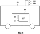
- This model can be stored in a non-volatile memory, as represented on figure 5 .
- FIG. 5 is a schematic representation of a vehicle 200, here a car, equipped with a system 201 for performing an object detection using LIDAR point clouds acquired by a LiDAR system (emitter 202A and receiver 202B).
- System 201 comprises a processor 203 and a non-volatile memory 204 in which the trained model has been stored.
Landscapes
- Physics & Mathematics (AREA)
- Engineering & Computer Science (AREA)
- Computer Networks & Wireless Communication (AREA)
- Electromagnetism (AREA)
- General Physics & Mathematics (AREA)
- Radar, Positioning & Navigation (AREA)
- Remote Sensing (AREA)
- Optical Radar Systems And Details Thereof (AREA)
Abstract
determining (DET_R0) the initial range, an initial intensity value (DET_I), the product of the optical constant and the pulse peak power (DET_CaP0),
determining (DET_I1) a first intensity value by attenuating the initial intensity value,
determining (DET_I2(R)) a set of values each associated with a range,
identifying (ID_I2R) the greatest value of the set, and the associated range,
obtaining a second intensity corresponding to the backscattering using at least the greatest value,
if (I2>I1) the second intensity value is greater than the first,
- determining a random value,
- replacing the position of the point using the identified range and the random value,
- replacing the intensity of the point with the second intensity value, else, replacing the intensity of the point with the first intensity value.
Description
- The present disclosure is related to the field of LiDAR point clouds, and more precisely to the processing of these point clouds so as to simulate the acquisition of a LiDAR point cloud of this scene in the presence of an aerosol, for example an aerosol of liquid particles (or solid particles), typically fog (aerosol of water particles).
- Light detection and ranging (LiDAR) is a method for determining the distance between a light emitter and an object.
- In particular, LiDAR is crucial for the implementation of safe autonomous cars, because LiDAR measures the precise distance of objects from the sensor, which image (RGB) cameras cannot measure directly. Thus, LiDAR has found its way into many applications, including detection, tracking, localization, and mapping. Despite the benefit of measuring exact depth information, LiDAR has a significant drawback. The light pulses that LiDAR sensors emit in the invisible near infrared (NIR) spectrum (typically at 850 and 903 to 905 nm wavelength) do not penetrate water particles, or other types of aerosol particles, as opposed to automotive radars. This means that as soon as there are water particles in the form of fog in the air (or other types of aerosols), light pulses emitted by the sensor will undergo backscattering and attenuation.
Attenuation reduces the received signal power that corresponds to the range of the solid object in the line of sight which should be measured, while backscattering creates a spurious peak in the received signal power at an incorrect range. As a result, the acquired LiDAR point cloud will contain some spurious returns whenever there is fog present at the time of capture. This poses a big challenge for most outdoor applications, as they typically require robust performance under all weather conditions. - In recent years, several LiDAR datasets for 3D object detection have been presented. Although many of them contain diverse driving scenarios, none of them allows an evaluation on different kinds of adverse weather. Only recently, the Canadian Adverse Driving Conditions Dataset (CADCD) (Matthew Pitropov, Danson Garcia, Jason Rebello, Michael Smart, Carlos Wang, Krzysztof Czarnecki, and Steven Waslander. Canadian adverse driving conditions dataset, 2020) and the Seeing Through Fog (STF) Dataset (Mario Bijelic, Tobias Gruber, Fahim Mannan, Florian Kraus, Werner Ritter, Klaus Dietmayer, and Felix Heide. Seeing through fog without seeing fog: Deep multimodal sensor fusion in unseen adverse weather. In The IEEE Conference on Computer Vision and Pattern Recognition (CVPR), June 2020.) address the need for such an evaluation. While CADCD focuses on snowfall, STF is targeted towards evaluation under fog, rain and snow. Consequently, there is still not a large quantity of LiDAR foggy data available that could be used to train deep neural networks.
- In fact, collecting and annotating large-scale datasets per se is time, labor and cost intensive, let alone when done for adverse weather conditions.
-
Figure 1A is a photography of a scene on which a vehicle, a barrier, and a bank are visible, although fog is present. -
Figure 1B is a representation of a LiDAR point cloud for the scene offigure 1A . It can be observed that the bank forms a dense cloud on the left side of the vehicle, because as a solid object, it reflects LiDAR pulses efficiently. On the right side of the vehicle (and above the barrier which is outside the LiDAR system's field of view directly next to the vehicle), the absence of any solid object leads to LiDAR responses from the fog floating around the vehicle (the small cloud around the vehicle). This results from the fact that the fog caused LiDAR responses and acts as an object which will provide the strongest response in the absence of a solid object. - While difficult to represent here, an attenuation of intensity can also be observed.
- The known techniques are still not satisfactory.
- The present disclosure overcomes one or more deficiencies of the prior art by proposing a method for processing a LiDAR point cloud of a scene so as to simulate the acquisition of a LiDAR point cloud of this scene in the presence of an aerosol, comprising, for every point of the LiDAR point cloud:
- a. determining the initial range of this point,
- b. determining an initial intensity value associated with this point,
- c. determining the product of the LiDAR system's optical constant and of the LiDAR pulse peak power sent by the LiDAR emitter,
- d. determining a first intensity value (this first intensity value can be called the attenuated intensity value) for this point by multiplying the intensity value determined in step b, by a factor depending on an attenuation coefficient (set at the desired aerosol density level for each simulation) and on the initial range determined in step a (i.e. an intensity is calculated for the object already present in the scene which produced a point: a hard object),
- e. determining a set of values each associated with a range comprised between 0 and the initial range determined in step a (the ranges can increase from 0 to the range of step a with a given step, for example 10 cm), by calculating an integral over time of predetermined relationship between the range (the one comprised between 0 and the initial range), the initial range determined in step a, the attenuation coefficient, and the half-power pulse width of the LiDAR emitter (used to acquire the LiDAR point cloud - the emitter is comprised within a LiDAR system including an emitter and a receiver),
- f. identifying the greatest value of the set of values, and the associated range,
- g. multiplying the value identified in step f by the product determined in step c and a backscattering coefficient (for example a constant set by an operator), to obtain a second intensity value corresponding to the backscattering produced by the aerosol (the second intensity value can be called a backscatter intensity value),
- h. if the second intensity value identified in step g is greater than the first intensity value determined in step d,
- determining a random value,
- replacing the position of the point with a position determined using the range identified in step f and the random value (the random value ensures that the position is arranged randomly around the point corresponding to this range - a new point cloud is obtained and instead of the initial point, there is now a point with a position comprised substantially between the original point and the receiver),
- replacing the intensity of the point with the second intensity value obtained in step g (the new point has an intensity depending on the integration of predetermined relationship),
- The point cloud used as input can preferably be acquired under clear weather, which the person skilled in the art will identify as the absence of aerosol. Alternatively, a light level of aerosol or fog can be present. The person skilled in the art will be able to identify the presence of points owing to backscattering in the point cloud used as input, which may indicate that a point cloud cannot be used as input.
- It has been observed that a good simulation of the presence of aerosol can be obtained by determining two different intensity values, as it reflects the effect of an aerosol such as fog: the signal can be attenuated but originate from the initial object, or the aerosol itself will produce a peak through backscattering. In other words, the present method is based on the physical effect that fog has on LiDAR.
- If the backscattered peak is greater than the attenuated peak, the backscattered peak should be kept and its location can be used to determine the location of the new point which replaces the initial point in the LIDAR point cloud. This operation has been observed to be in accordance with how LiDAR system produces points (each point is associated with a peak in the received signal).
- The person skilled in the art can implement the first intensity value using the attenuation coefficient and the initial range. For example, this can be done using a function, or a set of pre-calculated values (for example obtained using LiDAR point clouds acquired under fog).
- Also, the person skilled in the art will know how to define the attenuation coefficient. By way of example, document "Semantic foggy scene understanding with synthetic data" (Christos Sakaridis, Dengxin Dai, and Luc Van Gool. International Journal of Computer Vision, 126(9):973-992, Sep 2018) uses an analogous attenuation coefficient in the context of fog.
- The product of the LiDAR system optical constant and of the LiDAR pulse peak power sent by the LiDAR emitter can be obtained using values provided by the manufacturer of the LiDAR system, or they can be deduced from a measurement by the LiDAR system. Also, the LiDAR system optical constant is known to the person skilled in the art as not depending on range or time but on the aperture area of the sensor and given by CA = cηAR /2, wherein c is the speed of light, η characterizes the losses in the receiver's optics and AR is the aperture area of the sensor's optical receiver.
- According to a particular embodiment, the values obtained by integrating the predetermined relationship are stored in a lookup table (having multiple entries in particular for the range, the initial range, and the parameters of the predetermined relationship).
- The values stored in this lookup table can be calculated in a preliminary step. This embodiment diminishes the computing burden.
- According to a particular embodiment, the integral of step e is the one of the following relationship


- CA is the optical constant of the LiDAR system,
- P 0 is the LiDAR pulse peak power sent by the LiDAR emitter,
- β is the backscattering coefficient,
- τH is the half-power pulse width of the LiDAR emitter,
- t is the time,
- α is the attenuation coefficient,
- c is the speed of light,
- ξ() is the crossover function defining the ratio of the area illuminated by the LIDAR emitter and the part of it observed by the receiver,
- U() is the Heaviside function, and
- R 0 is the initial range determined in step a.
- The above equation has been observed to be a good representation of the received power (from which the intensity can be deduced as they are linearly linked) resulting from backscattering at different ranges.
- This equation has been obtained using the linear system model of document "Influences of weather phenomena on automotive laser radar systems" (R. Rasshofer, M. Spies, and H. Spies. Advances in Radio Science, 9, 07 2011) which describes the received signal power at a LiDAR receiver, which is valid for non-elastic scattering. This equation notably takes into account the spatial impulse response of the LiDAR optical system in foggy conditions.
- It should be noted that the integral in this equation (the one of step e) can be used to obtain values stored in said lookup table, or it can be used to perform on the fly computations.
- The above equation also includes the multiplication by CAP 0β which is performed in step g, but preferably only for the greatest value (alternatively for all values).
- According to a particular embodiment, the integral of step e is calculated using an approximate method.
- According to a particular embodiment, Simpson's rule is used as approximate method.
- This method has been observed to be a suitable numerical integration method for the invention.
- According to a particular embodiment, step d comprises calculating the first intensity value using the following equation:

- i is the initial intensity value,
- α is the attenuation coefficient, and
- R 0 is the initial range determined in step a.
- This equation has been observed to be a good representation of the received power for an object (here a solid/hard object) when an aerosol is present.
- According to a particular embodiment, the method comprises processing a plurality of LiDAR point clouds each associated with labels (typically the position in space of objects and their types), to obtain a processed machine learning training dataset comprising the processed LiDAR point clouds and the corresponding labels.
- The invention further provides a method of training a machine learning detection model using the training dataset obtained previously to detect the labels.
- The simulation of aerosol improves the training of a machine learning detection model configured to receive LiDAR point clouds as input.
- The invention also provides a system comprising a LiDAR system and, stored on a recording medium readable by a computer, the neural network trained in accordance with the method as defined above.
- The invention also provides a vehicle comprising a system as defined above.
- In one particular embodiment, the steps of the method are determined by computer program instructions.
- Consequently, the invention is also directed to a computer program for executing the steps of a method as described above when this program is executed by a computer.
- This program can use any programming language and take the form of source code, object code or a code intermediate between source code and object code, such as a partially compiled form, or any other desirable form.
- The invention is also directed to a computer-readable information medium containing instructions of a computer program as described above.
- The information medium can be any entity or device capable of storing the program. For example, the medium can include storage means such as a ROM, for example a CD ROM or a microelectronic circuit ROM, or magnetic storage means, for example a diskette (floppy disk) or a hard disk.
- Alternatively, the information medium can be an integrated circuit in which the program is incorporated, the circuit being adapted to execute the method in question or to be used in its execution.
- Further features and advantages of the present disclosure will become apparent from the following description of certain embodiments thereof, given by way of illustration only, not limitation, with reference to the accompanying drawings in which:
-
Figure 1A and 1B , already described, represent a scene in which fog is present. -
Figure 2 is a schematic representation of a LIDAR optical system. -
Figure 3A and 3B are two graphs illustrating the received power as computed according to an example. -
Figure 4 is a schematic representation of the steps of a method for processing LIDAR point clouds according to an example. -
Figure 5 is a schematic representation of a vehicle according to an example. - We will now describe a method for processing a LiDAR point cloud of a scene so as to simulate the acquisition of a LiDAR point cloud of this scene in the presence of an aerosol.
- In the present description, homogeneous fog is used as the exemplary aerosol. The present invention is however not limited to fog and can be adapted to other homogeneous aerosols (for example fumes, etc.).
- From document "Influences of weather phenomena on automotive laser radar systems", a linear system model is known to describe the received signal power at a LiDAR's receiver, under the assumption that the scattering is non-elastic. In particular, the received signal power PR as a function of range R (the distance between an object and the receiver) is modeled as the time-wise convolution of the transmitted signal power PT with the spatial impulse response H of the optical system:

- Wherein c is the speed of light, CA is the optical constant of the LiDAR system, R is the range, and t is the time.
- More precisely, CA is a constant not depending on range or time but on the aperture area of the sensor and given by CA = cηAR /2, wherein c is the speed of light, η characterizes the losses in the receiver's optics and AR is the aperture area of the sensor's optical receiver.
- It should be noted that while the above equation provides an expression of the received power, the associated intensity can be deduced from this power as they are linearly linked.
- Now, we will describe and model the remaining terms. From the above document, it is known that the time signature of the transmitted pulse can be modeled by a squared sine function:

- Wherein P 0 is the emitted pulse's peak power and τH is the half-power pulse width, and t is the time.
- From the above mentioned document "Influences of weather phenomena on automotive laser radar systems", τH is usually known to be comprised between 10 and 20 nanoseconds. In equation 2, the time origin is not set at the peak of the pulse, which typically corresponds to the acquired range measurement, but at the start of the pulse, so that all signals are set at zero for negative time values. In the following, this convention is kept and the required correction to the range is performed when necessary. For example, when subsequently a set of ranges has to be considered, the correction can include going from


- The spatial impulse response function H of the optical system can be modeled as the product of the individual impulse responses of the optical channel, HC, and of the target (i.e. the actual object) HT :

- And the impulse response of the optical channel HC is:

- Wherein T(R) is the total one-way transmission loss and ξ(R) is the crossover function defining the ratio of the area illuminated by the transmitter and the part of it observed by the receiver, as represented on
Figure 2 , where a bistatic beam configuration is used. By way of example, ξ(R) can be expressed using the following piece-wise linear approximation:
- Wherein R1, visible on
figure 2 , indicates the range at which the two beams start to overlap, and R2, visible onfigure 2 , indicates the range at which the two beams fully overlap. More precisely,figure 2 is a schematic representation of a LiDAR sensor system equipped with a transmitter Tx and a receiver Rx which do not have coaxial optics but parallel axes. This configuration is called a bistatic beam configuration. - Further, the total one-way transmission loss T(R) is defined as:

- Wherein α(r) is a spatially varying attenuation coefficient, corresponding to a fog density level. As the fog is considered to be homogeneous, α(r) = α, with α being a selected/given fog density level.
- Consequently:

- It should be noted that the attenuation coefficient α increases as visibility range decreases. Therefore, for a same three-dimensional scene, the impulse response of the optical channel HC varies with visibility.
- Also, the last term in
equation 1 that remains to be modeled is the impulse response of the target HT. However, different cases should be considered for HT according to the weather conditions, as the composition of the target for the same three-dimensional scene is different under fog than in clear weather. The present method proposes to construct a relation between the response PR in clear weather and in fog for the same three-dimensional scene and this relation enables the simulation of fog (or other aerosols) on clear-weather LiDAR point clouds. - Further, the previously described optical model is particularized for clear weather cases and fog in terms of impulse response terms HC and HT.
- Under clear weather, the attenuation coefficient α is zero, which leads to:

- Moreover, the target in clear weather is comprised only of the solid object on which the LiDAR pulse is reflected. This type of target is called a hard target.
- The impulse response HT of a hard target at range R 0 is a Dirac delta function expressed as:

- Wherein β 0 denotes the differential reflectivity of the target. If only diffuse reflections (Lambertian surfaces) are considered, β 0 is expressed as:

- Wherein Γ is the reflectivity comprised between 0 and 1.
- Consequently, in clear weather the total impulse response function H(R) can be expressed as:

- Wherein the property ƒ(x)δ(x - x 0) = ƒ(x 0)δ(x - x 0) has been applied. Because in practice R 2 is less than two meters, it is assumed that R 2 ≪ R 0, which leads to ξ(R 0) = 1. Thus, starting from
equation 1 and given the range measurement R 0 obtained from an initial clear weather LiDAR point cloud, the received signal power can be computed in closed form as:
- The received signal power attains its maximum value at


- The next step is to establish the transformation of PR,clear(R) to PR,fog(R), the received power under fog. While the same hard target still exists since the three-dimensional scene is the same, there is now an additional contribution from the fog itself, which constitutes a soft target, as explained in document "Influences of weather phenomena on automotive laser radar systems", that provides distributed scattering to the impulse response HT.
- The impulse response of this soft fog target is expressed as:

- Wherein β denotes the backscattering coefficient, which is constant under the assumption that the fog is homogeneous, and U is the Heaviside function. In equation 13, the function,

- The co-existence of a soft target and a hard target can be modeled by considering the superposition of the respective impulse responses:

- Consequently, in fog, the total impulse response function H(R) can be expressed as:

- It has been observed that compared to clear weather, the spatial impulse response in fog is more complex to compute, but it can still be decomposed into two terms, corresponding to the hard and soft target respectively, leading to a respective decomposition of the received response as:

- Focusing on the hard target term, and using
equation 1 to calculate the corresponding term of the received response

- Thus, the hard target term of the response in fog is an attenuated version of the clear-weather response PR,clear. On the other hand, the soft target term is expressed as:

- Equation 18 does not possess a closed-form expression, as the integral I(R,R 0 ,α,τH ) on the right-hand side of equation 18 cannot be calculated analytically.
- However, for a given τH and a given α (which can be set according to a desired density level of fog by an operator), I(R,R 0,α,τH ) can be computed numerically for fixed values of R. By way of example, Simpson's 1/3 rule for numerical integration can be used to provide an approximation of the profile of

-
Figure 3A and 3B are illustrations of both

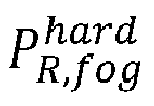

figure 3A , the fog is not thick enough to yield a return due to backscatter, while onfigure 3B , the fog is thick enough to yield a return due to backscatter that overshadows the solid object at R 0 = 30m. As the LIDAR receiver usually places a point into the point cloud associated with the greatest peak in the received signal, it follows that forfigure 3A , the range is unchanged and the power should be calculated in accordance with equation 17, while forfigure 3B , the range and the position of the point in space should both be changed in accordance with equation 18. - In fact, depending on the distance of the hard target from the sensor, the soft target term of the response may exhibit a larger maximum value than the hard target term, which implies that the measured range changes due to the presence of fog and becomes equal to the point of maximum of the soft target term.
- It should be noted that the parameters of
equations 1 to 18 can be defined in accordance with a given LiDAR system. By way of example, a LiDAR system commercialized by the American company Velodyne Lidar under the reference HDL-64E can be considered. This leads to a half-pulse width τH of 20 nanoseconds. Also, β can be set to

- From
equations 1 to 18, it is possible to conceive a method, implemented on a computer, which will take a LiDAR point cloud of a scene as input, and simulate the acquisition of a LiDAR point cloud of the same scene in the presence of an aerosol such as fog, for every point of the LiDAR point cloud. - On
figure 4 , an exemplary method is represented. This method comprises, for every point of the LiDAR point cloud (under clear weather), an initial step DET_R0 wherein the initial range R 0 of this point is determined. Typically, the point has three coordinates to define its position in space. From these coordinates, it is possible to determine the initial range. - In a second step DET_I, the initial intensity value i associated with the point is determined. This intensity is provided along with the LIDAR point cloud.
- Then, the product of the LiDAR system optical constant and of the LiDAR pulse peak power sent by the LiDAR emitter are determined in step DET_CaP0. This corresponds to obtaining the product CAP 0, which can be provided by the manufacturer of the LiDAR system, or deduced from
equation 12. In fact, using the intensity i and the range R 0 of the point and a selected value of β 0, it is possible to deduce this product. - From this initial intensity value i, a first intensity value, for example denoted ihard for this point is determined in step DET_I1. This is performed using equation 17 (adapted for intensities), and comprises multiplying the intensity value determined in step DET_I, by a factor depending on the attenuation coefficient α and on the initial range R 0 determined in step DET_R0.
- In a subsequent step DET_I2(R) (which could also be performed before DET_I1), a set of values each associated with a range comprised between 0 and the range determined in step a, by calculating an integral over time of a predetermined relationship between the range R, the initial range R 0 determined in step a, the attenuation coefficient α, and the half-power pulse width τH of the LiDAR emitter. In other words, this step comprises determining I(R,R 0 ,α,τH ), for example for ranges spaced apart by 10cm, and also for example by using Simpson's rule.
- Alternatively, step DET_I2(R) comprises using a lookup table in which the values have been predetermined.
- Then, in step ID_I2R, the greatest value itmp of the set of values is identified, as well as the associated range Rtmp.
- A multiplication is then carried out (step MULT) wherein the value itmp identified in step ID_I2R is multiplied by the product determined in step DET_CaP0 and the backscattering coefficient β, to obtain a second intensity value isoft corresponding to the backscattering produced by the aerosol.
- A comparison is then performed in step I2>I1. If the second intensity value isoft is greater than the first intensity value ihard, then the soft target has produced a greater LiDAR response than the hard target (similar to
figure 3B ). - Step REPL_I2 is then carried out in which:
- A random value is determined (to avoid having a precise sphere of points associated with the fog/the soft target),
- The position of the point (the initial point of the LIDAR point cloud) is replaced with a position determined using the range Rtmp identified in step ID_I2R, and the random value.
- The intensity of the point (the initial point of the LIDAR point cloud) is replaced with the second intensity isoft obtained in step MULT.
- By way of example obtaining a random value can comprise obtaining a random value p comprised within -1 and 1 (of type float). A noise factor n = 2 p can then be calculated which will be used with a scaling factor


- The point is then replaced in the LIDAR point cloud.
- If the first intensity ihard is superior or equal to the second intensity isoft, the position of the point is unchanged but the first intensity value ihard is used as the new intensity value of the point.
- By way of example, it is possible to process the point clouds from a dataset of LiDAR point clouds acquired under clear weather, for which labels are known, to obtain a training dataset.
- From this training dataset, a machine learning detection model such as the PV-RCNN (Shaoshuai Shi, Chaoxu Guo, Li Jiang, Zhe Wang, Jianping Shi, Xiaogang Wang, and Hongsheng Li. Pv-rcnn: Point-voxel feature set abstraction for 3d object detection. In Proceedings of the IEEE/CVF Conference on Computer Vision and Pattern Recognition, pages 10529-10538, 2020) can be trained to obtain a trained machine learning detection model to detect objects.
- This model can be stored in a non-volatile memory, as represented on
figure 5 . -
Figure 5 is a schematic representation of avehicle 200, here a car, equipped with asystem 201 for performing an object detection using LIDAR point clouds acquired by a LiDAR system (emitter 202A andreceiver 202B).System 201 comprises aprocessor 203 and anon-volatile memory 204 in which the trained model has been stored. - It should be noted that the detection of various objects (cars, cyclists, pedestrians) has been improved when training a detection model with the processed point clouds of the present method, in particular, the detection is improved over the fog simulation of document "Seeing through fog without seeing fog: Deep multimodal sensor fusion in unseen adverse weather" (Mario Bijelic, Tobias Gruber, Fahim Mannan, Florian Kraus, Werner Ritter, Klaus Dietmayer, and Felix Heide. In The IEEE Conference on Computer Vision and Pattern Recognition (CVPR), June 2020).
- Throughout the description, including the claims, the term "comprising a" should be understood as being synonymous with "comprising at least one" unless otherwise stated. In addition, any range set forth in the description, including the claims should be understood as including its end value(s) unless otherwise stated. Specific values for described elements should be understood to be within accepted manufacturing or industry tolerances known to one of skill in the art, and any use of the terms "substantially" and/or "approximately" and/or "generally" should be understood to mean falling within such accepted tolerances.
- Although the present disclosure herein has been described with reference to particular embodiments, it is to be understood that these embodiments are merely illustrative of the principles and applications of the present disclosure.
- It is intended that the specification and examples be considered as exemplary only, with a true scope of the disclosure being indicated by the following claims.
Claims (12)
- A computer implemented method for processing a LiDAR point cloud of a scene so as to simulate the acquisition of a LiDAR point cloud of this scene in the presence of an aerosol, comprising, for every point of the LIDAR point cloud:a. determining (DET_R0) the initial range of this point,b. determining (DET_I) an initial intensity value associated with this point,c. determining (DET_CaP0) the product of the LiDAR system's optical constant and of the LiDAR pulse peak power sent by the LiDAR emitter,d. determining (DET_I1) a first intensity value for this point by multiplying the intensity value determined in step b, by a factor depending on an attenuation coefficient and on the initial range determined in step a,e. determining (DET_I2(R)) a set of values each associated with a range comprised between 0 and the initial range determined in step a, by calculating an integral over time of a predetermined relationship between the range, the initial range determined in step a, the attenuation coefficient, and the half-power pulse width of the LiDAR emitter,f. identifying (ID_I2R) the greatest value of the set of values, and the associated range,g. multiplying the value identified in step f by the product determined in step c and a backscattering coefficient, to obtain a second intensity value corresponding to the backscattering produced by the aerosol,h. if (I2>I1) the second intensity value identified in step g is greater than the first intensity value determined in step d,else, replacing the intensity of the point with the first intensity value determined in step d.- determining a random value,- replacing the position of the point with a position determined using the range identified in step f and the random value,- replacing the intensity of the point with the second intensity value obtained in step g,
- The method of claim 1, wherein the values obtained by integrating the predetermined relationship are stored in a lookup table.
- The method of claim 1 or 2, wherein the integral of step e is the one of the following relationship

 CA is the optical constant of the LIDAR system,P 0 is the LiDAR pulse peak power sent by the LiDAR emitter,β is the backscattering coefficient,τH is the half-power pulse width of the LiDAR emitter,t is the time,α is the attenuation coefficient,c is the speed of light,ξ() is the crossover function defining the ratio of the area illuminated by the LiDAR emitter and the part of it observed by the receiver,U() is the Heaviside function, andR 0 is the initial range determined in step a.
 - The method of claim 3, wherein the integral is calculated using an approximation method (e.g. numerical integration).
- The method of claim 4, wherein Simpson's rule is used as approximation method.
- The method of any one of claims 1 to 5, wherein step d comprises calculating the first intensity value using the following equation:
 i is the initial intensity value,α is the attenuation coefficient, andR 0 is the initial range determined in step a.
 - The method of any one of claims 1 to 6, comprising processing a plurality of LIDAR point clouds each associated with labels, to obtain a processed machine learning training dataset comprising the processed LIDAR point clouds and the corresponding labels.
- A method of training a machine learning detection model using the training dataset obtained in claim 7 to detect the labels.
- A system comprising a LiDAR system and, stored on a recording medium readable by a computer, the neural network trained in claim 8.
- A vehicle comprising a system according to claim 9.
- A computer program including instructions for executing the steps of a method according to any one of claims 1 to 7 when said program is executed by a computer.
- A recording medium readable by a computer and having recorded thereon a computer program including instructions for executing the steps of a method according to any one of claims 1 to 7.
Priority Applications (1)
| Application Number | Priority Date | Filing Date | Title |
|---|---|---|---|
| EP21188957.1A EP4124888B1 (en) | 2021-07-30 | 2021-07-30 | A method for processing a lidar point cloud to simulate the presence of an aerosol such as fog |
Applications Claiming Priority (1)
| Application Number | Priority Date | Filing Date | Title |
|---|---|---|---|
| EP21188957.1A EP4124888B1 (en) | 2021-07-30 | 2021-07-30 | A method for processing a lidar point cloud to simulate the presence of an aerosol such as fog |
Publications (2)
| Publication Number | Publication Date |
|---|---|
| EP4124888A1 true EP4124888A1 (en) | 2023-02-01 |
| EP4124888B1 EP4124888B1 (en) | 2024-10-09 |
Family
ID=77274671
Family Applications (1)
| Application Number | Title | Priority Date | Filing Date |
|---|---|---|---|
| EP21188957.1A Active EP4124888B1 (en) | 2021-07-30 | 2021-07-30 | A method for processing a lidar point cloud to simulate the presence of an aerosol such as fog |
Country Status (1)
| Country | Link |
|---|---|
| EP (1) | EP4124888B1 (en) |
Cited By (1)
| Publication number | Priority date | Publication date | Assignee | Title |
|---|---|---|---|---|
| CN118961652A (en) * | 2024-10-21 | 2024-11-15 | 自然资源部第二海洋研究所 | A method for inverting the vertical structure of ocean subsurface optical properties based on ICESat-2 ATL03 global positioning photon data |
-
2021
- 2021-07-30 EP EP21188957.1A patent/EP4124888B1/en active Active
Non-Patent Citations (8)
| Title |
|---|
| BERNUTH ALEXANDER VON ET AL: "Simulating Photo-realistic Snow and Fog on Existing Images for Enhanced CNN Training and Evaluation", 2019 IEEE INTELLIGENT TRANSPORTATION SYSTEMS CONFERENCE (ITSC), IEEE, 27 October 2019 (2019-10-27), pages 41 - 46, XP033668733, DOI: 10.1109/ITSC.2019.8917367 * |
| CHRISTOS SAKARIDISDENGXIN DAILUC VAN GOOL: "Semantic foggy scene understanding with synthetic data", INTERNATIONAL JOURNAL OF COMPUTER VISION, vol. 126, no. 9, September 2018 (2018-09-01), pages 973 - 992 |
| GOODIN CHRISTOPHER ET AL: "Unmanned ground vehicle simulation with the Virtual Autonomous Navigation Environment", 2017 INTERNATIONAL CONFERENCE ON MILITARY TECHNOLOGIES (ICMT), IEEE, 31 May 2017 (2017-05-31), pages 160 - 165, XP033128462, DOI: 10.1109/MILTECHS.2017.7988748 * |
| MARIO BIJELICTOBIAS GRUBERFAHIM MANNANFLORIAN KRAUSWERNER RITTERKLAUS DIETMAYERFELIX HEIDE: "Seeing through fog without seeing fog: Deep multimodal sensor fusion in unseen adverse weather", THE IEEE CONFERENCE ON COMPUTER VISION AND PATTERN RECOGNITION (CVPR, June 2020 (2020-06-01) |
| R. RASSHOFERM. SPIESH. SPIES: "Influences of weather phenomena on automotive laser radar systems", ADVANCES IN RADIO SCIENCE, vol. 9, July 2011 (2011-07-01) |
| SAKARIDIS CHRISTOS ET AL: "Semantic Foggy Scene Understanding with Synthetic Data", INTERNATIONAL JOURNAL OF COMPUTER VISION, KLUWER ACADEMIC PUBLISHERS, NORWELL, US, vol. 126, no. 9, 23 March 2018 (2018-03-23), pages 973 - 992, XP036568429, ISSN: 0920-5691, [retrieved on 20180323], DOI: 10.1007/S11263-018-1072-8 * |
| SHAOSHUAI SHICHAOXU GUOLI JIANGZHE WANGJIANPING SHIXIAOGANG WANGHONGSHENG LI.: "Pv-rcnn: Point-voxel feature set abstraction for 3d object detection", PROCEEDINGS OF THE IEEE/CVF CONFERENCE ON COMPUTER VISION AND PATTERN RECOGNITION, 2020, pages 10529 - 10538 |
| ZHAO JIAN ET AL: "Method and Applications of Lidar Modeling for Virtual Testing of Intelligent Vehicles", IEEE TRANSACTIONS ON INTELLIGENT TRANSPORTATION SYSTEMS, IEEE, PISCATAWAY, NJ, USA, vol. 22, no. 5, 10 March 2020 (2020-03-10), pages 2990 - 3000, XP011851568, ISSN: 1524-9050, [retrieved on 20210430], DOI: 10.1109/TITS.2020.2978438 * |
Cited By (1)
| Publication number | Priority date | Publication date | Assignee | Title |
|---|---|---|---|---|
| CN118961652A (en) * | 2024-10-21 | 2024-11-15 | 自然资源部第二海洋研究所 | A method for inverting the vertical structure of ocean subsurface optical properties based on ICESat-2 ATL03 global positioning photon data |
Also Published As
| Publication number | Publication date |
|---|---|
| EP4124888B1 (en) | 2024-10-09 |
Similar Documents
| Publication | Publication Date | Title |
|---|---|---|
| Hahner et al. | Fog simulation on real LiDAR point clouds for 3D object detection in adverse weather | |
| US7616817B2 (en) | Three dimensional shape correlator | |
| CN111369617B (en) | 3D target detection method of monocular view based on convolutional neural network | |
| Rosenberger et al. | Benchmarking and functional decomposition of automotive lidar sensor models | |
| CN112986964B (en) | Photon counting laser point cloud self-adaptive denoising method based on noise neighborhood density | |
| Dannheim et al. | Weather detection in vehicles by means of camera and LIDAR systems | |
| CN113378760A (en) | Training target detection model and method and device for detecting target | |
| CN109213138B (en) | Obstacle avoidance method, device and system | |
| US20210018611A1 (en) | Object detection system and method | |
| US20200398797A1 (en) | Vehicle sensor enhancements | |
| US20210044366A1 (en) | Estimating strength of radio frequency signal | |
| CN110542909A (en) | Atmospheric visibility detection method and electronic equipment | |
| TWI735191B (en) | System and method for lidar defogging | |
| Prio et al. | Implementation of dynamic radius outlier removal (dror) algorithm on lidar point cloud data with arbitrary white noise addition | |
| EP4124888A1 (en) | A method for processing a lidar point cloud to simulate the presence of an aerosol such as fog | |
| Wu et al. | The YOLO-based multi-pulse lidar (YMPL) for target detection in hazy weather | |
| Godfrey et al. | Evaluation of flash LiDAR in adverse weather conditions toward active road vehicle safety | |
| CN116299231B (en) | A radar data simulation method, apparatus, electronic device, and storage medium | |
| CN113256483A (en) | De-dithering of point cloud data for target identification | |
| US12481025B2 (en) | Object sensing device and object sensing method | |
| CN113640764B (en) | Radar one-dimensional range profile identification method and device based on multi-dimension one-dimensional convolution | |
| Zhan et al. | Towards visibility estimation and noise-distribution-based defogging for LiDAR in autonomous driving | |
| Park et al. | New approach to sea surface wind retrieval from GNSS-R measurements | |
| EP4235214A1 (en) | Lidar snowfall simulation method and system for robust 3d object detection | |
| Holder et al. | How to evaluate synthetic radar data? Lessons learned from finding driveable space in virtual environments |
Legal Events
| Date | Code | Title | Description |
|---|---|---|---|
| PUAI | Public reference made under article 153(3) epc to a published international application that has entered the european phase |
Free format text: ORIGINAL CODE: 0009012 |
|
| STAA | Information on the status of an ep patent application or granted ep patent |
Free format text: STATUS: REQUEST FOR EXAMINATION WAS MADE |
|
| 17P | Request for examination filed |
Effective date: 20210730 |
|
| AK | Designated contracting states |
Kind code of ref document: A1 Designated state(s): AL AT BE BG CH CY CZ DE DK EE ES FI FR GB GR HR HU IE IS IT LI LT LU LV MC MK MT NL NO PL PT RO RS SE SI SK SM TR |
|
| RIC1 | Information provided on ipc code assigned before grant |
Ipc: G01S 17/00 20200101ALI20240315BHEP Ipc: G01S 17/89 20200101AFI20240315BHEP |
|
| GRAP | Despatch of communication of intention to grant a patent |
Free format text: ORIGINAL CODE: EPIDOSNIGR1 |
|
| STAA | Information on the status of an ep patent application or granted ep patent |
Free format text: STATUS: GRANT OF PATENT IS INTENDED |
|
| INTG | Intention to grant announced |
Effective date: 20240522 |
|
| GRAS | Grant fee paid |
Free format text: ORIGINAL CODE: EPIDOSNIGR3 |
|
| GRAA | (expected) grant |
Free format text: ORIGINAL CODE: 0009210 |
|
| STAA | Information on the status of an ep patent application or granted ep patent |
Free format text: STATUS: THE PATENT HAS BEEN GRANTED |
|
| AK | Designated contracting states |
Kind code of ref document: B1 Designated state(s): AL AT BE BG CH CY CZ DE DK EE ES FI FR GB GR HR HU IE IS IT LI LT LU LV MC MK MT NL NO PL PT RO RS SE SI SK SM TR |
|
| REG | Reference to a national code |
Ref country code: CH Ref legal event code: EP |
|
| REG | Reference to a national code |
Ref country code: DE Ref legal event code: R096 Ref document number: 602021019819 Country of ref document: DE |
|
| REG | Reference to a national code |
Ref country code: IE Ref legal event code: FG4D |
|
| REG | Reference to a national code |
Ref country code: LT Ref legal event code: MG9D |
|
| REG | Reference to a national code |
Ref country code: NL Ref legal event code: MP Effective date: 20241009 |
|
| REG | Reference to a national code |
Ref country code: AT Ref legal event code: MK05 Ref document number: 1731147 Country of ref document: AT Kind code of ref document: T Effective date: 20241009 |
|
| PG25 | Lapsed in a contracting state [announced via postgrant information from national office to epo] |
Ref country code: NL Free format text: LAPSE BECAUSE OF FAILURE TO SUBMIT A TRANSLATION OF THE DESCRIPTION OR TO PAY THE FEE WITHIN THE PRESCRIBED TIME-LIMIT Effective date: 20241009 |
|
| PG25 | Lapsed in a contracting state [announced via postgrant information from national office to epo] |
Ref country code: NL Free format text: LAPSE BECAUSE OF FAILURE TO SUBMIT A TRANSLATION OF THE DESCRIPTION OR TO PAY THE FEE WITHIN THE PRESCRIBED TIME-LIMIT Effective date: 20241009 |
|
| PG25 | Lapsed in a contracting state [announced via postgrant information from national office to epo] |
Ref country code: HR Free format text: LAPSE BECAUSE OF FAILURE TO SUBMIT A TRANSLATION OF THE DESCRIPTION OR TO PAY THE FEE WITHIN THE PRESCRIBED TIME-LIMIT Effective date: 20241009 Ref country code: PT Free format text: LAPSE BECAUSE OF FAILURE TO SUBMIT A TRANSLATION OF THE DESCRIPTION OR TO PAY THE FEE WITHIN THE PRESCRIBED TIME-LIMIT Effective date: 20250210 Ref country code: IS Free format text: LAPSE BECAUSE OF FAILURE TO SUBMIT A TRANSLATION OF THE DESCRIPTION OR TO PAY THE FEE WITHIN THE PRESCRIBED TIME-LIMIT Effective date: 20250209 |
|
| PG25 | Lapsed in a contracting state [announced via postgrant information from national office to epo] |
Ref country code: FI Free format text: LAPSE BECAUSE OF FAILURE TO SUBMIT A TRANSLATION OF THE DESCRIPTION OR TO PAY THE FEE WITHIN THE PRESCRIBED TIME-LIMIT Effective date: 20241009 |
|
| PG25 | Lapsed in a contracting state [announced via postgrant information from national office to epo] |
Ref country code: BG Free format text: LAPSE BECAUSE OF FAILURE TO SUBMIT A TRANSLATION OF THE DESCRIPTION OR TO PAY THE FEE WITHIN THE PRESCRIBED TIME-LIMIT Effective date: 20241009 |
|
| PG25 | Lapsed in a contracting state [announced via postgrant information from national office to epo] |
Ref country code: ES Free format text: LAPSE BECAUSE OF FAILURE TO SUBMIT A TRANSLATION OF THE DESCRIPTION OR TO PAY THE FEE WITHIN THE PRESCRIBED TIME-LIMIT Effective date: 20241009 |
|
| PG25 | Lapsed in a contracting state [announced via postgrant information from national office to epo] |
Ref country code: NO Free format text: LAPSE BECAUSE OF FAILURE TO SUBMIT A TRANSLATION OF THE DESCRIPTION OR TO PAY THE FEE WITHIN THE PRESCRIBED TIME-LIMIT Effective date: 20250109 |
|
| PG25 | Lapsed in a contracting state [announced via postgrant information from national office to epo] |
Ref country code: LV Free format text: LAPSE BECAUSE OF FAILURE TO SUBMIT A TRANSLATION OF THE DESCRIPTION OR TO PAY THE FEE WITHIN THE PRESCRIBED TIME-LIMIT Effective date: 20241009 Ref country code: GR Free format text: LAPSE BECAUSE OF FAILURE TO SUBMIT A TRANSLATION OF THE DESCRIPTION OR TO PAY THE FEE WITHIN THE PRESCRIBED TIME-LIMIT Effective date: 20250110 Ref country code: AT Free format text: LAPSE BECAUSE OF FAILURE TO SUBMIT A TRANSLATION OF THE DESCRIPTION OR TO PAY THE FEE WITHIN THE PRESCRIBED TIME-LIMIT Effective date: 20241009 |
|
| PG25 | Lapsed in a contracting state [announced via postgrant information from national office to epo] |
Ref country code: PL Free format text: LAPSE BECAUSE OF FAILURE TO SUBMIT A TRANSLATION OF THE DESCRIPTION OR TO PAY THE FEE WITHIN THE PRESCRIBED TIME-LIMIT Effective date: 20241009 |
|
| PG25 | Lapsed in a contracting state [announced via postgrant information from national office to epo] |
Ref country code: RS Free format text: LAPSE BECAUSE OF FAILURE TO SUBMIT A TRANSLATION OF THE DESCRIPTION OR TO PAY THE FEE WITHIN THE PRESCRIBED TIME-LIMIT Effective date: 20250109 |
|
| PG25 | Lapsed in a contracting state [announced via postgrant information from national office to epo] |
Ref country code: SM Free format text: LAPSE BECAUSE OF FAILURE TO SUBMIT A TRANSLATION OF THE DESCRIPTION OR TO PAY THE FEE WITHIN THE PRESCRIBED TIME-LIMIT Effective date: 20241009 |
|
| PG25 | Lapsed in a contracting state [announced via postgrant information from national office to epo] |
Ref country code: DK Free format text: LAPSE BECAUSE OF FAILURE TO SUBMIT A TRANSLATION OF THE DESCRIPTION OR TO PAY THE FEE WITHIN THE PRESCRIBED TIME-LIMIT Effective date: 20241009 |
|
| REG | Reference to a national code |
Ref country code: DE Ref legal event code: R097 Ref document number: 602021019819 Country of ref document: DE |
|
| PG25 | Lapsed in a contracting state [announced via postgrant information from national office to epo] |
Ref country code: EE Free format text: LAPSE BECAUSE OF FAILURE TO SUBMIT A TRANSLATION OF THE DESCRIPTION OR TO PAY THE FEE WITHIN THE PRESCRIBED TIME-LIMIT Effective date: 20241009 |
|
| PG25 | Lapsed in a contracting state [announced via postgrant information from national office to epo] |
Ref country code: RO Free format text: LAPSE BECAUSE OF FAILURE TO SUBMIT A TRANSLATION OF THE DESCRIPTION OR TO PAY THE FEE WITHIN THE PRESCRIBED TIME-LIMIT Effective date: 20241009 |
|
| PG25 | Lapsed in a contracting state [announced via postgrant information from national office to epo] |
Ref country code: SK Free format text: LAPSE BECAUSE OF FAILURE TO SUBMIT A TRANSLATION OF THE DESCRIPTION OR TO PAY THE FEE WITHIN THE PRESCRIBED TIME-LIMIT Effective date: 20241009 |
|
| PG25 | Lapsed in a contracting state [announced via postgrant information from national office to epo] |
Ref country code: CZ Free format text: LAPSE BECAUSE OF FAILURE TO SUBMIT A TRANSLATION OF THE DESCRIPTION OR TO PAY THE FEE WITHIN THE PRESCRIBED TIME-LIMIT Effective date: 20241009 |
|
| PG25 | Lapsed in a contracting state [announced via postgrant information from national office to epo] |
Ref country code: IT Free format text: LAPSE BECAUSE OF FAILURE TO SUBMIT A TRANSLATION OF THE DESCRIPTION OR TO PAY THE FEE WITHIN THE PRESCRIBED TIME-LIMIT Effective date: 20241009 |
|
| PLBE | No opposition filed within time limit |
Free format text: ORIGINAL CODE: 0009261 |
|
| STAA | Information on the status of an ep patent application or granted ep patent |
Free format text: STATUS: NO OPPOSITION FILED WITHIN TIME LIMIT |
|
| PG25 | Lapsed in a contracting state [announced via postgrant information from national office to epo] |
Ref country code: SE Free format text: LAPSE BECAUSE OF FAILURE TO SUBMIT A TRANSLATION OF THE DESCRIPTION OR TO PAY THE FEE WITHIN THE PRESCRIBED TIME-LIMIT Effective date: 20241009 |
|
| 26N | No opposition filed |
Effective date: 20250710 |
|
| PGFP | Annual fee paid to national office [announced via postgrant information from national office to epo] |
Ref country code: DE Payment date: 20250604 Year of fee payment: 5 |
|
| REG | Reference to a national code |
Ref country code: CH Ref legal event code: H13 Free format text: ST27 STATUS EVENT CODE: U-0-0-H10-H13 (AS PROVIDED BY THE NATIONAL OFFICE) Effective date: 20260224 |
|
| PG25 | Lapsed in a contracting state [announced via postgrant information from national office to epo] |
Ref country code: LU Free format text: LAPSE BECAUSE OF NON-PAYMENT OF DUE FEES Effective date: 20250730 |
|
| GBPC | Gb: european patent ceased through non-payment of renewal fee |
Effective date: 20250730 |
|
| REG | Reference to a national code |
Ref country code: BE Ref legal event code: MM Effective date: 20250731 |
|
| PG25 | Lapsed in a contracting state [announced via postgrant information from national office to epo] |
Ref country code: GB Free format text: LAPSE BECAUSE OF NON-PAYMENT OF DUE FEES Effective date: 20250730 |
|
| PG25 | Lapsed in a contracting state [announced via postgrant information from national office to epo] |
Ref country code: BE Free format text: LAPSE BECAUSE OF NON-PAYMENT OF DUE FEES Effective date: 20250731 |
|
| PG25 | Lapsed in a contracting state [announced via postgrant information from national office to epo] |
Ref country code: FR Free format text: LAPSE BECAUSE OF NON-PAYMENT OF DUE FEES Effective date: 20250731 |
|
| PG25 | Lapsed in a contracting state [announced via postgrant information from national office to epo] |
Ref country code: CH Free format text: LAPSE BECAUSE OF NON-PAYMENT OF DUE FEES Effective date: 20250731 |