EP4123519A1 - System and computer-implemented method for dynamic adaption of automotive functions - Google Patents
System and computer-implemented method for dynamic adaption of automotive functions Download PDFInfo
- Publication number
- EP4123519A1 EP4123519A1 EP21187378.1A EP21187378A EP4123519A1 EP 4123519 A1 EP4123519 A1 EP 4123519A1 EP 21187378 A EP21187378 A EP 21187378A EP 4123519 A1 EP4123519 A1 EP 4123519A1
- Authority
- EP
- European Patent Office
- Prior art keywords
- model
- generalized
- prediction
- vehicle
- federated
- Prior art date
- Legal status (The legal status is an assumption and is not a legal conclusion. Google has not performed a legal analysis and makes no representation as to the accuracy of the status listed.)
- Granted
Links
Images

Classifications
-
- G—PHYSICS
- G06—COMPUTING OR CALCULATING; COUNTING
- G06N—COMPUTING ARRANGEMENTS BASED ON SPECIFIC COMPUTATIONAL MODELS
- G06N20/00—Machine learning
- G06N20/20—Ensemble learning
Definitions
- each vehicle needs to decide how and when to update both models, i.e. the generalized federated model f FL and the personalized model f k .
- Each decision unit needs to decide which of the above-mentioned models to choose from for prediction ⁇ .
- the vehicle k of vehicles receives a globally trained model, i.e. the generalized federated model f FL from the Backend.
- each edge 110 A ... 110 N, 210 A ... 210 N is locally optimizing the locally stored model. Rather than transmitting locally accessed/generated data to the Backend 130, 230, each edge 110 A ... 110 N, 210 A ... 210 N is only transmitting update parameters, e.g. from the computational unit 120 A ... 120 N, 220 A ... 220 N to the Backend 130, 230.
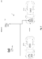
- Figure 2 shows an exemplary system 200 improving the efficiency in security in dynamic adaption of automotive functions for a plurality of vehicles 210 A ... 210 N in a highly dynamic external and internal environment.
- the system 200 is in accordance with the system 100 as explained with reference to Figure 1 above for the generalized federated model f FL , and comprises the following additional features.
- TOSM Time-Optimised Smoothed Model
Landscapes
- Engineering & Computer Science (AREA)
- Theoretical Computer Science (AREA)
- Software Systems (AREA)
- Data Mining & Analysis (AREA)
- Evolutionary Computation (AREA)
- Medical Informatics (AREA)
- Computer Vision & Pattern Recognition (AREA)
- Physics & Mathematics (AREA)
- Computing Systems (AREA)
- General Engineering & Computer Science (AREA)
- General Physics & Mathematics (AREA)
- Mathematical Physics (AREA)
- Artificial Intelligence (AREA)
- Management, Administration, Business Operations System, And Electronic Commerce (AREA)
Abstract
Description
- The present invention relates to a system and computer-implemented method for improving the efficiency and security in dynamic adaption of automotive functions.
- In modern vehicular environments, sensor date, image data, audio data etc. from an environment of a vehicle and a vehicle cabin are accessed and processed in order to provide intelligent vehicle functions and to enhance data management of the vehicle. In order to efficiently and reliably process the above-mentioned data, huge amounts of a plurality of vehicles need to be processed. Such an environment of data generated by a plurality of vehicles that comprise context-aware, real-time systems in the sense of ubiquitous computing, can be summarized as real-time distributed system. The transmission of the generated data towards the Backend for generating intelligent vehicle functions is even with the use of new technologies in mobile networks (e.g. 5G) costly and requires enormous storage and processing power. Therefore in-vehicle processing is required and efficient transferring of data needed. Moreover, due to the increase of in-vehicle applications and due to the fact that data accessed comprises sensitive, personal data, there is a need to perform data computation, data analytics and machine-learning near the data source - in the sense of Edge Computing - rather than by a Backend - in the sense of Cloud Computing. Each vehicle can be considered to represent an edge device in the sense of Edge Computing. In order to preserve data privacy, it is known to apply Federated Learning. Federated Learning has been introduced within the context of Edge Computing, aiming to solve edge learning under privacy sensitive, non-independent and identically distributed (non-i.i.d.), and unbalanced data generated from massively distributed devices using the technique of machine learning. Federated Learning within this document is a machine learning setting where multiple entities (clients) collaborate in solving a machine learning problem, under the coordination of a central server or service provider. Each client's raw data is stored locally and not exchanged or transferred; instead, focused updates intended for immediate aggregation are used to achieve the learning objective. The main drawback of Federated Learning in the context of an automotive application is, that the learning model according to Federated Learning is at some point considered to be optimized. However, vehicles as edge devices are highly dynamic and the data changes dynamically with the dynamic vehicle environment and vehicle interior situation. Therefore, the model can never be considered to be optimized. Moreover, for intelligent vehicle functions and around the autonomous driving context, the usage of personal and local behaviour adaption of the model is of high importance. Mainly because a generalized model from the Backend cannot provide the most accurate and best qualitative results a personal adapted model can do, towards the individual local environment the vehicle is placed at.
- It is an object of the present invention to overcome the above-mentioned drawbacks by providing a solution that enables a dynamic, efficient and secure adaptation of automotive functions.
- This problem is solved by the independent claims. Preferred embodiments are described in the dependent claims.
- According to a first aspect of the invention, a system for improving the efficiency and security in dynamic adaptation of an automotive application in a vehicle is provided. The system comprises:
- a Backend comprising a generalized federated model fFL deployed thereon,
- wherein the vehicle is operable to receive and deploy the generalized federated model fFL in a first computational unit;
- wherein the vehicle is operable to deploy a personalized model fk in a second computational unit; and
- wherein the vehicle comprises a decision unit that is operable to locally decide, for a prediction ŷ of the automotive application, which of the generalized federated model fFL and the personalized model fk to use;
- calculating, by the decision unit, the prediction ŷ using the decided model; and adapting the automotive application based on the prediction ŷ.
- The Backend comprises a generalized federated model fFL deployed thereon. The System can be an Edge Computing System where Federated Learning is applied at the Backend. Within this application, an Edge Computing System is a distributed system where different entities are connected to communicate with each other forming a network. Throughout this document, Edge Computing can be understood as processing the data at an Internet of Things (IoT)-device level. IoT is a ubiquitous computing paradigm in which everyday objects, e.g. vehicles, are enriched with embedded computational power towards monitoring the environment by collecting data without any user interaction in real-time. The collected data is processed and analyzed to generate knowledge. In the sense of Edge Computing, the Backend is represented as one level, but can be extended towards a plurality of levels or tiers, respectively, forming a complex hierarchy of the architecture. Processing and computation is moved further towards the devices level, wherein each device or edge is a vehicle. Accordingly, the latency, the computational power, and the storage of the Backend decreases. On the other hand, bandwidth, privacy, and responsiveness increases by pushing the intelligence and processing towards the vehicles instead of the Backend. Enabling computation, decision making, and intelligence at the vehicles provides the ability to perform machine learning in the vehicles close to the data sources collected by a plurality of well-known sensors, allowing to build low-latency and location-aware applications with keeping the privacy of the data collected and/or generated in each of the vehicles. Generally, the data collected and/or generated at the vehicles and the gained intelligence through machine learning can be used to support and improve the underlying infrastructure and management or to enable in-vehicle applications and services. Such services and applications supported by machine-learning techniques in the sense of Edge Computing can be found in the area of autonomous driving and/or autonomous driving use cases.
- Federated Learning (FL) is a state of the art - approach for applying machine learning in edges, with reference to the above-mentioned system in the vehicles. Federated Learning has been introduced within the context of Edge Computing, aiming to solve the problem of machine-learning in edges under privacy sensitive data generated from massively distributed devices. According to the Federated Learning - Paradigm, multiple edges collaborate in solving a machine learning problem, under the coordination of the central Backend. Each vehicle's raw data is stored locally, in a storage device of one or more computational units of each respective vehicle and not exchanged or transferred to the Backend. Rather, focused updates intended for immediate aggregation are used to achieve the learning objective.
- Each vehicle receives and deploys one global model, the generalized federated model fFL, that is globally trained by the central Backend. To do so, the Backend transmits the generalized federated model fFL via a Network, e.g. the mobile network, to each of the vehicles. Each vehicle is storing and deploying the globally trained generalized federated model fFL received from the Backend locally, e.g. in the storage device of the computational unit. With the locally generated/accessed data, each vehicle is locally optimizing the locally stored model. Rather than transmitting locally accessed/generated data to the Backend, each vehicle is transmitting update parameters, e.g. from the computational unit to the Backend.
- In an exemplary implementation, Federated Learning (FL) - as applied by the Backend is a distributed machine learning optimization problem in a network of vehicles. The aim is to locally optimize an objection function J over distributed datasets. In the following, the vehicles will be also referred to as Edge Devices. In the following, the generation and updating of the generalized federated model fFL in the Backend and the Edge Devices is explained in more detail:
A network of k ∈ {1,...,k,...,K} of Edge Devices is designed with each holding a local subset of data Dk so that D = {D 1,...,Dk ,...,DK }. - This dataset Dk is generated through Sensing and Actuating Nodes (SANs) sensing continuously contextual data in form of a d-dimensional vector x t with



Each time t a new contextual vector Xt is received at the Edge Device. In centralized learning this data is forwarded to the Backend that minimizes the objective functionover the entire dataset D. The optimization of the loss function
 over a training set D of size N using a set of models


- In FL the optimization of the functionis performed by locally optimizing an objective function
 in each Edge Device k over the local dataset Dk with length nk so that

The Backend is aggregating the local generated objective functions Jk so that: (xi ,yi ,w) or local optimization function
 (w) can be also noted as
 ji (w). One exemplary algorithm to solve the problem of Equation (5.2) is using the Stochastic Gradient Descent (SGD). Each iteration t the Edge Device (ED) k aims to converge towards the minimum loss function
 , over its local data Dk at time t given a new datapoint Xt . This is by adapting the model parameters


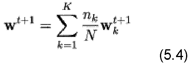
- The Federated Learning algorithm within the Backend aggregates the received model parameters inside the central coordinator towards the new generalized model. This averaging is summarised in Equation 5.4.

- As outlined above, only implementing Federated Learning introduces multiple drawbacks within an application for an automotive environment. The first issue is the adaption of the generalized model - i.e. the final federated model distributed to the Edge Devices- to constantly changing environments in a vehicular context - e.g. highly dynamic environment, highly dynamic situation in the vehicle interior, etc. - in which the assumption of converging to a global minimization of the objective functiondoes not hold. The second problem arises as each Edge Device k always overwrites the locally adapted model fFL with a newly received generalized federated model fFL, such that locally learned context for each Edge Device is lost.

- Moreover, with only applying Federated Learning, the global, final federated model is - at some point - considered to be optimized and is no longer updated by the Backend. However, when using machine learning in Edge Device environments and in particular in the automotive environment where each vehicle represents an Edge Device, the main challenge is the highly heterogeneous nature of the vehicles, resulting in non-i.i.d. data and evolving environment with possible concept drifts of the data collected by the vehicles.
- In order to solve the above-mentioned problems, each vehicle further deploys a personalized model fk in a second computational unit locally in the respective vehicle.
- In other words, each vehicle k has deployed two models, the above-mentioned generalized federated model fFL, received from the Backend, in a first computational unit and, in parallel, an evolving personalized model fk in a second computational unit.
- Each vehicle comprises a decision unit that is operable to locally decide, for a prediction ŷ of the automotive application, which of the generalized federated model fFL and the personalized model fk to use;
- For each prediction of a relevant automotive application - for example with reference to autonomous driving - a decision unit locally decides which of the personalized model fk or the generalized federated model fFL is the most accurate model to be used for the prediction ŷ:

- Since each vehicle has limited resources, complex algorithms for the decision making cannot be used. Therefore, a lightweight method for balancing the personalized model fk and the generalized federated model fFL needs to be applied. In other words, since the vehicles resources are limited, a complex machine learning algorithm cannot be implemented for the decision making. Therefore, each vehicle of the system needs to apply continuous data prediction, forecasting and monitoring of the decision making process.
- Moreover, each vehicle needs to decide how and when to update both models, i.e. the generalized federated model fFL and the personalized model fk. Each decision unit needs to decide which of the above-mentioned models to choose from for prediction ŷ. As outlined above, at epoch s, the vehicle k of vehicles receives a globally trained model, i.e. the generalized federated model fFL from the Backend.
- In a next step, the decision unit of the vehicle calculates the prediction ŷ using the decided model i.e. either the generalized federated model fFL or the personalized model fk.
- Finally, the automotive application is adapted by an appropriate control unit of the vehicle based on the prediction ŷ.
- According to an embodiment of the invention, the decision unit, when locally deciding which of the generalized federated model fFL and the personalized model fk to use for the prediction ŷ, and when performing the prediction ŷ, performs the following steps:
- calculating a prediction error εk for the local, personalized model fk deployed in the second computational unit;
- calculating a prediction error εFL for the generalized federated model fFL deployed in the first computational unit;
- calculating a reward value θ for the calculated prediction error εk and εFL
- considering a historical performance of the local, personalized model fk and the generalized federated model fFL ; and
- calculating the prediction ŷ by balancing the prediction of the local, personalized model fk and the generalized federated model fFL.
- As outlined above, each vehicle k has deployed two models, the generalized federated model fFL in the first computational unit and, in parallel, the evolving personalised model fk in the second computational unit. For each prediction ŷ of a relevant automotive application - for example with reference to autonomous driving - the decision unit locally decides which of the personalized model fk or the generalized federated model fFL is the best model to be used for the prediction y:

- As outlined above, at epoch s, the vehicle k of vehicles receives the globally trained model, i.e. the generalized federated model fFL from the Backend.
- As also outlined above, in order to enable a global update for the generalized federated model fFL, k vehicles perform over its locally stored data in a SLW Wk the update parameters using Equation (5.3). These updates are forwarded to the Backend and used into the new (a globally trained) model by combining all selected k vehicles update parameters, as shown in Equation (5.4). In a next step, each vehicle receives the new globally trained model, i.e. the updated generalized federated model fFL which can be used for prediction ŷ to perform the predictive analytics locally.
- The personalized model fk is set to be at t = 0 the centrally received generalized federated model fFL. The choice of using a pre-build model as starting point lies in the theories of transfer learning, which highlights that using a baseline model for retraining is generating an earlier convergence and higher accuracy than starting from scratch. SANs continuously measures the surrounding of each vehicle and generates respective measurement data. Each vehicle receives this measurement data from the SANs at each time
t with

- In contrast, the personalized model fk is updated and retrained each time t at the vehicle using a local SGD process.
- One main technical advantage and keeping both models inside the vehicles is mainly to overcome the problem of losing generalization and the adaption to unseen data by only deploying a personal model. Moreover, the previously unknown relationship between the vehicles in evolving systems can be changing from an i.i.d. to a non-i.i.d. data relationship. This leads towards better accuracy to the generalized model or personalized model depending on the connection. Using a balancing mechanism of the generalized and personalized model inside each vehicle provides the benefits of both data relations towards qualitative prediction results.
- The methodology presented in this application contributes towards the solution of the above-mentioned problems by using a reward system for choosing the right model for the prediction. In particular, the decision unit of vehicle k is operable to weigh the personalized model fk and generalized federated model fFL to generate a combined prediction ŷ. The final prediction ŷ is calculated locally in each vehicle k of vehicles by using the local personalized model fk and the generalized federated model fFL with an adaptive balancing weight α. The prediction ŷ is performed/calculated locally in a decision unit of the respective vehicle.
- The decision unit is operable to perform the steps of
- calculating a prediction error εk for the local, personalized model fk deployed in the second computational unit; and
- calculating a prediction error εFL for the generalized federated model fFL deployed in the first computational unit. To do so, the adaptive weight is calculated through multiple steps. First, whenever a vehicle receives from the SANs a new contextual vector xt at time t, the prediction error εk for the local, personalized model fk with respect to the actual prediction yt and the prediction error εFL for the generalized federated model fFL is calculated as shown in Equation (5.5) and (5.6), respectively.



- As shown in Equation (5.7), a positive reward is given to the generalized federated model fFL if the absolute error εFL is smaller than the absolute error εk of the personalized model fk. As the reward system is deployed inside the respective vehicle 210 A ... 210 N should not only incorporate the current performance of the two models but also the historical performance, the reward-values θ at each time t are stored in a Sliding Window (SLW) 0k with size U for the last t - U times. The SLW is defined in Equation (5.8) and contains just zeros and ones:

- The SLW Ok consists of the most recent U rewards of θ ∈ {0, 1}. At each time t, the SLW of rewards is used as a reference to generate a ratio that represents the performance of both models over the time horizon t - U. This ratio is defining the adaptive weighting value α. An exemplary computation of a can be seen in Equation (5.9) and represents the historical performance of both models inside a respective vehicle.

- Each time t vehicle k is performing a prediction ŷ, the two model predictions of the personalized model fk and the generalized federated model fFL are weighted to the final prediction ŷ. The adaptive value α is used to combine the generalized federated model fFL and the local personalized model fk towards ŷ. The balancing of these two models is defined as shown in Equation (5.10):

- An exemplary implementation algorithm for the above-mentioned steps is as follows: Backend 230:wherein ED is the respective vehicle 210 A ... 210N
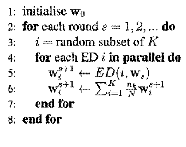
- Respective vehicle 210 A ... 210 N (run at each vehicle k), wherein CL is the Backend 230:

- The value range of α is between 1 and 0. A value of α → 1 means more influence towards the model predictions coming of the generalized federated model fFL, whereas a value of α → 0 places more importance on the locally generated predictions of the personalized model fk .
- According to a further embodiment of the invention, the decision unit, when locally deciding which of the generalized federated model fFL and the personalized model fk to use for the prediction ŷ, and when performing the prediction ŷ, performs the following steps:
- calculating a prediction error εk for the local, personalized model fk deployed in the second computational unit;
- calculating a prediction error εFL for the generalized federated model fFL deployed in the first computational unit;
- calculating a best time time t* to switch from the generalized federated model fFL to the personalized model fk or to switch from the personalized model fk to the generalized federated model fFL taking into account the calculated prediction error εk and the calculated prediction error εFL ;
- considering a historical performance of the generalized federated model fFL to the personalized model fk ; and
- calculating the prediction ŷ by balancing the prediction error εk of the local, personalized model fk and the prediction error εFL of the generalized federated model fFL.
- An alternative approach for choosing one of the generalized federated model fFL and the personalized model fk can be performed by the applying the Time-Optimised Smoothed
- Model (TOSM) by the decision unit of vehicle k. TOSM introduces the concept of Optimal Stopping Theory (OST). Instead of weighting the predictions, as outlined above, one model is chosen for the prediction ŷ by identifying the optimal model at time t.
- To do so, each vehicle k of vehicles at time t calculates for the personalized model fk and generalized federated model fFL the prediction error εFL and the prediction error εk , respectively, as defined in Equations (5.5) and (5.6) outlined above.
- At time t = s = 0 the chosen model inside the vehicle k is the generalized federated model fFL. Given the prediction error εFL and the prediction error εk, the decision unit 240 A ... 240 N decides when the best time t* is to switch from the generalized federated model fFL to the personalized model fk. In a next step, the concept of Optimal Stopping Theory (OST) is used and performed on the prediction error εFL and the prediction error εk as performance value.
- Each time t the prediction error εFL and the prediction error εk are compared and rewarded as binary value Z. The binary variable Z is introduced as highlighted in Equation (5.11).

- Zt is defined as 0 if the personalized model fk is generating a higher prediction error than the generalized federated model fFL. If the personalized model fk is, however, generating a lower prediction error εk in comparison to the generalized federated model fFL, the value of Zt is set to 1.
- When vehicle k is deciding instantly based on the given comparison the personalized model fk and the generalized federated model fFL at time t to switch the model, no historical behaviour is incorporated towards this decision. As previous behaviour and prediction quality are of importance to most automotive applications, the values of the cumulative sum of comparison, including the history divergence of these two models, are used as switching decision. The instruct history of rewarded prediction performance comparison is then calculated by the cumulative sum of Zt defined as Rt and introduced in the following Equation:

- The accumulated sum of Zt defined as Rt is used to find the optimal time to decide when to switch from the generalized federated model fFL to the personalized model fk. Therefore the reward function for switching the generalized federated model fFL to the personalized model fk is defined in Equation (5.13) using the quantity of Rt . The value of β indicates the delay tolerance level with β ∈ (0, 1). If β → 1, the delay is increased:

- Finding the optimal time t* the reward function Yt as outlined in Equation (5.13) is used by maximizing the expectation of Yt with expectation E[Yt ] having a fixed delay tolerance of β. Formally, this can be described as finding the supremum of the expectation of Yt as, given the following Equation:

- The optimal time t* for switching from the generalized federated model fFL to the personalized model fk can be defined as:

- The expectation E[Z] can be calculated with the formulation of Zt in Equation (5.11) to the summation of the expectation


- As the expectation of Z is given Equation (5.11) set to


- During a training period for the application the Probability Density Function (PDF) of the prediction error εFL and the prediction error εk can be obtained, which leads to generate the optimal time t* for switching from the generalized federated model fFL to the personalized model fk :

- The introduced methodology of TOSM is further considering the reverse switching from the generalized federated model fFL to the personalized model fk. Therefore, once the model is switched from the generalized federated model fFL to the personalized model fk, the time value of R is set to 0. Then the concept of finding the optimal time t* to switch back from the personalized model fk to the generalized federated model fFL with using the same concept as previous is starting inside the vehicle k of vehicles 210 A ... 210 N. The optimal time to switch from the personalized model fk to the generalized federated model fFL is made through the variable Q in which the prediction error εFL and the prediction error εk for both models are monitored. Similar to the variable Zt, Qt is calculated as:

- From Equation (5.19), the expectation of Q using the methodologies of Equation (5.17) and (5.18) from lead to:

- From the given expectation of Q in Equation (5.20), it is possible to derive the optimal time t* to switch from the local personalized model fk back to the generalized federated model fFL. Only the Probability Density Function (PDF) of the error values of the prediction error εFL and the prediction error εk is needed and can be generated through a training period of the application inside the respective vehicle k of vehicles 120 A ... 120 N. In Equation (5.21), the optimal time t* for the switch is defined. Once the model is switched back to the generalized federated model fFL, the summation of values of Q is reset, and the Z accumulation is starting. This method is performed until a new globally trained
model 232 is received from theBackend 230, replacing the old generalized federated model fFL as new generalized federated model fFL. This provokes a reset and a starting of using Z with the new generalized federated model fFL.
- According to a further embodiment of the invention, the dynamic adaptation of the automotive application comprises one or more of the following:
- adapting any function of any driving assistance system application of the vehicle based on the calculated prediction value ŷ;
- adapting any function of any autonomous driving system application of the vehicle based on the calculated prediction value ŷ; and/or
- adapting any function of any infotainment system application of the vehicle based on the calculated prediction value ŷ; and/or
- adapting any appropriate function of any system application of the vehicle based on the calculated prediction value ŷ.
- Considering as an example a function of a driving style of a user of the vehicle, a behavior or mood detection algorithm using audio, video and other sensor data inside the car can be used as input factors for generating the above-explained function. Based on the prediction value ŷ for the driving style/mood/behavior of the user of the vehicle, one possibility for an above-mentioned driving assistance system application can be the adaption of speed and distance control of the vehicle after the function/prediction identified a tired or distracted driver as user of the vehicle. This increases safety and security while the driving. Further it is possible to adapt the infotainment system towards stimulus music or individual interior light design given a drivers mood and behavior as user of the vehicle to either e.g. calm a stressed driver down or wakeup a tired driver with their favorite dance music. Moreover but not limited, can be the adaption towards autonomous driving applications by using a predefined selection of driving modes (e.g. eco, electric,...), routes (coffee shop, restaurant, scenic drive,...) or routines (call a certain person, reserve a treatment,...) given the learning and prediction of the personal preferences towards a certain environment.
- According to another aspect of the invention, a computer-implemented method for improving the efficiency and security in dynamic adaptation of an automotive application in a vehicle is provided. The method comprises the following steps
- receiving and deploying, from a Backend, a generalized federated model fFL in a first computational unit of the vehicle;
- deploying a personalized model fk in a second computational unit of the vehicle;
- locally deciding, by a decision unit of the vehicle, for a prediction ŷ of the automotive application, which of the generalized federated model fFL and the personalized model fk to use;
- calculating, by the decision unit the prediction ŷ based on the decided model; and
- adapting the automotive application, by the vehicle based on the prediction ŷ.
- According to an embodiment of the invention, the locally deciding, by the decision unit, which of the generalized federated model fFL and the personalized model fk to use for the prediction ŷ, and the performing of the prediction ŷ comprises the steps of:
- calculating a prediction error εk for the local, personalized model fk deployed in the second computational unit;
- calculating a prediction error εFL for the generalized federated model fFL deployed in the first computational unit;
- calculating a reward value θ for the calculated prediction error εk and εFL
- considering a historical performance of the local, personalized model fk and the generalized federated model fFL ; and
- calculating the prediction ŷ by balancing the prediction of the local, personalized model fk and the generalized federated model fFL
- According to a further embodiment of the invention, the locally deciding, by the decision unit which of the generalized federated model fFL and the personalized model fk to use for the prediction ŷ, and the performing of the prediction ŷ comprises the steps of:
- calculating a prediction error εk for the local, personalized model fk deployed in the second computational unit;
- calculating a prediction error εFL for the generalized federated model fFL deployed in the first computational unit;
- calculating a best time time t* is to switch from the generalized federated model fFL to the personalized model fk or to switch from the personalized model fk to the generalized federated model fFL taking into account the calculated prediction error εk and the calculated prediction error εFL ;
- considering a historical performance of the generalized federated model fFL to the personalized model fk ; and
- performing the prediction ŷ by balancing the prediction error εk of the local, personalized model fk and the prediction error εFL of the generalized federated model fFL.
- According to yet a further embodiment of the invention, the dynamic adaptation of the automotive application comprises one or more of the following:
- adapting any function of any driving assistance system application of the vehicle based on the calculated prediction value ŷ;
- adapting any function of any autonomous driving system application of the vehicle based on the calculated prediction value ŷ; and/or
- adapting any function of any infotainment system application of the vehicle based on the calculated prediction value ŷ; and/or
- adapting any appropriate function of any system application of the vehicle based on the calculated prediction value ŷ
- The aspects defined above and further aspects of the present invention are apparent from the examples of embodiment to be described hereinafter and are explained with reference to the examples of embodiment. The invention will be described in more detail hereinafter with reference to examples of embodiment. However, it is apparent to the person skilled in the art that the invention is not limited to the examples of embodiment.
- Figure 1
- shows an exemplary Edge Computing System where Federated Learning is applied;
- Figure 2
- shows an exemplary system for improving the efficiency and security in dynamic adaptation of an automotive application in a vehicle;
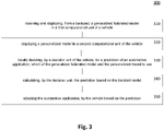
- Figure 3
- shows an exemplary method for improving the efficiency and security in dynamic adaptation of an automotive application in a vehicle.
-
Figure 1 shows an exemplaryEdge Computing System 100 where Federated Learning is applied. Within this application, an Edge Computing System is a distributed system where different entities are connected to communicate with each other forming a network. Throughout this document, Edge Computing can be understood as processing the data at an Internet of Things (IoT)-device level. IoT is a ubiquitous computing paradigm in which everyday objects, e.g. vehicles 110 A ... 110 N, 210 A ... 210 N, are enriched with embedded computational power towards monitoring the environment by collecting data without any user interaction in real-time. The collected data is processed and analyzed to generate knowledge. In the sense of Edge Computing,Backend 130 is represented as one level, but can be extended towards a plurality of levels or tiers, respectively, forming a complex hierarchy of the architecture. Processing and computation is moved further towards the devices level, wherein each device or edge is a vehicle 110 A ... 110 N, 210 A ... 210 N. Accordingly, the latency, the computational power, and the storage of theBackend 130 decreases. On the other hand, bandwidth, privacy, and responsiveness increases by pushing the intelligence and processing towards the vehicles 110 A ... 110 N, 210 A ... 210 N instead of theBackend 130. Enabling computation, decision making, and intelligence at the edges 110 A ... 110 N, 210 A ... 210 N provides the ability to perform machine learning in the edge devices or vehicles 110 A ... 110 N, 210 A ... 210 N close to the data sources, allowing to build low-latency and location-aware applications with keeping the privacy of the data collected and/or generated in each of the vehicles. Generally, the data collected and/or generated at edge devices / vehicles 110 A ... 110 N, 210 A ... 210 N and the gained intelligence through machine learning can be used to support and improve the underlying infrastructure and management or to enable in-vehicle applications and services. Such services and applications supported by machine-learning techniques in the sense of Edge Computing can be found in the area of autonomous driving and/or autonomous driving use cases. - Federated Learning (FL) is a state of the art - approach for applying machine learning in edges 110 A ... 110 N, 210 A ... 210 N. Federated Learning has been introduced within the context of Edge Computing, aiming to solve the problem of machine-learning in edges 110 A ... 110 N, 210 A ... 210 N under privacy sensitive data generated from massively distributed devices. According to the Federated Learning - Paradigm, multiple edges 110 A ... 110 N, 210 A ... 210 N collaborate in solving a machine learning problem, under the coordination of a
central Backend 130. Each edge's raw data is stored locally, e.g. in a storage device of a computational unit 110 A ... 110 N, 210 A ... 210 N and not exchanged or transferred to theBackend 130. Rather, focused updates intended for immediate aggregation are used to achieve the learning objective. Each edge 110 A ... 110 N, 210 A ... 210 N receives and deploys oneglobal model 132 that is globally trained by thecentral Backend 130. TheBackend model 132 via a Network, e.g. themobile network model 132 received from theBackend Backend Backend - In an exemplary implementation, Federated Learning (FL) - as applied by the
Backend - A network of k ∈ {1,...,k,...,K} of Edge Devices 110 A ... 110 N, 210 A ... 210 N is designed with each holding a local subset of data Dk so that D = {D 1,...,Dk ,...,D K }.
- This dataset Dk is generated through Sensing and Actuating Nodes (SANs) sensing continuously contextual data in form of ad-dimensional vector xt with


Backend 130 that minimizes the objective functionover the entire dataset D. The optimization of the loss function (x, y; w) can be approximated by exploring the Empirical Risk Minimization (ERM) instead of the expected risk. Therefore, an approximation of
 over a training set D of size N using a set of models


- In FL the optimisation of the functionis performed by locally optimizing an objective function
 in each Edge Device k 110 A ... 110 N, 210 A ... 210 N over the local dataset Dk with length nk so that

- The
Backend  (xi ,yi ,w) or local optimization function
 (w) can be also noted as ji (w). One exemplary algorithm to solve the problem of Equation (5.2) is using the Stochastic Gradient Descent (SGD). Each iteration t the Edge Device (ED) k aims to converge towards the minimum loss function
 , over its local data Dk at time t given a new datapoint Xt. This is by adapting the model parameters


Backend - The Federated Learning algorithm within the
Backend 
Backend federated model 132 is distributed to the Edge Devices 110 A ... 110 N, 210 A ... 210 N and used locally for inference. Each ED k is selected at a random time epochs with s = {1, ... , s, ... , S} to update the distributed federated model fFL with its local data stored in a Sliding Window
Backend - As outlined above, an implementation of Federated Learning introduces multiple drawbacks within an application for an automotive environment. The first issue is the adaption of the generalized model - i.e. the final
federated model 132 distributed to the Edge Devices fFL - to constantly changing environments in a vehicular context - e.g. highly dynamic environment, highly dynamic situation in the vehicle interior, etc. - in which the assumption of converging to a global minimization of the objective functiondoes not hold. The second problem arises as each Edge Device 110 A ... 110 N always overwrites the locally adapted model f̂FL with a newly received generalized model fFL, such that locally learned context for each Edge Device 110 A ... 110 N is lost.
- Moreover, with the application of Federated Learning, the global, final
federated model 132 is - at some point - considered to be optimized and is no longer updated by theBackend 130. However, when using machine learning in edge device environments and in particular in the automotive environment where each vehicle 110 A ... 110 N represents an edge-device, the main challenge is the highly heterogeneous nature of the vehicles, resulting in non-i.i.d. data and continuous evolving of the data collected by the vehicles 110 A ... 110 N. This problem, however, cannot be addressed by only using the above-explained Federated Learning. -
Figure 2 shows anexemplary system 200 improving the efficiency in security in dynamic adaption of automotive functions for a plurality of vehicles 210 A ... 210 N in a highly dynamic external and internal environment. Thesystem 200 is in accordance with thesystem 100 as explained with reference toFigure 1 above for the generalized federated model fFL , and comprises the following additional features. - Each vehicle k 210 A ... 210 N has deployed two models, for example a generalized federated model fFL in a first computational unit 220 A ... 220 N and, in parallel, an evolving personalized model fk in a second computational unit 230 A ... 230 N. For each prediction of a relevant automotive application - for example with reference to autonomous driving - a decision unit 240 A ... 240 N, locally decides which of the personalized model fk or the generalized federated model fFL is the right model to be used for the prediction y:
ŷ with either ŷ = fFL (x) or ŷ = fk (x)
Since each vehicle 210 A ... 210 N has limited resources, complex algorithms for the decision making cannot be used. Therefore, a lightweight method for balancing the personalized model fk and the generalized federated model fFL needs to be applied. In other words, in vehicles 210 A ... 210 N, a complex machine learning algorithm cannot be implemented for the decision making. Therefore, each vehicle of the system needs to apply continuous data prediction, forecasting and monitoring of the decision making process. - Therefore, each vehicle 210 A ... 210 N needs to decide how and when to update both models, i.e. the generalized federated model fFL and the personalized model fk. Moreover, each decision unit 240 A ... 240 N needs to decide which of the above-mentioned models to choose from for prediction ŷ. As outlined with reference to
Figure 1 above, at epoch s, the vehicle k of vehicles 210 A ... 210 N receives a globally trainedmodel 232, i.e. the generalized federated model fFL from theBackend 230. - To do so, the vehicle k of vehicles 210 A ... 210 N performs over its locally stored data in a SLW Wk the update parameters using Equation (5.3). These updates are forwarded to the
Backend 230 and used into the new a globally trainedmodel 232 by combining all selected k vehicles 210 A ... 210 N update parameters, as shown in Equation (5.4). In a next step, each vehicle 210 A ... 210 N receive the new globally trainedmodel 232 which can be used for prediction ŷ to perform the predictive analytics locally. - The personalized model fk is set to be at t = 0 the centrally received generalized federated model fFL The choice of using a pre-build model as starting point lies in the theories of transfer learning, which highlights that using a baseline model for retraining is generating an earlier convergence and higher accuracy than starting from scratch. SANs continuously measures the surrounding of each vehicle 210 A ... 210 N and generates respective measurement data. Each vehicle 210 A ... 210 N receives this measurement data from the SANs at each time t with


- In contrast, the personalized model fk is updated and retrained each time t at the vehicle 210 A ... 210 N using a local SGD process.
- One main technical advantage and keeping both models inside the vehicles 210 A ... 210 N is mainly to overcome the problem of losing generalization and the adaption to unseen data by only deploying a personal model. Moreover, the previously unknown relationship between the vehicles in evolving systems can be changing from an i.i.d. to a non-i.i.d. data relationship. This leads towards better accuracy to the generalized model or personalized model depending on the connection. Using a balancing mechanism of the generalized and personalized model inside each vehicle provides the benefits of both data relations towards qualitative prediction results.
- The methodology presented in this application contributes towards the solution of the above-mentioned problem by using a reward system to weigh the personalized model fk and generalized federated model fFL combined prediction ŷ. The final prediction y is calculated locally in each vehicle k of vehicles 210 A ... 210 N by using the local personalized model fk and the generalized federated model fFL with a adaptive balancing weight α. The prediction ŷ is performed/calculated locally in a decision unit 240 A ... 240 N of the respective vehicle 210 A ... 210 N.
- The adaptive weight is calculated through multiple steps. First, whenever a vehicle 210 A ... 210 N receives from the SANs a new contextual vector xt at time t, the prediction error εk for the local, personalized model fk with respect to the actual prediction ŷt and the prediction error εFL for the generalized federated model fFL is calculated as shown in Equation (5.5) and (5.6), respectively.


- Given these two errors of Equation (5.5) and (5.6) inside each vehicle k of vehicles 210 A ... 210 N, it is possible to generate a reward value θ that is used as the source for balancing the personalized model fk and the generalized federated model fFL. In each vehicle k of vehicles 210 A ... 210 N at each time t based on the prediction error εFL and the prediction error εk a reward θ is set to 0 if the personalized model fk is performing better than the generalized federated model fFL. The reward θ is set to 1 if the generalized federated model fFL performs better, as is shown in the following Equation:

- As shown in Equation (5.7), a positive reward is given to the generalized federated model fFL if the absolute error εFL is smaller than the absolute error εk of the personalized model fk. As the reward system is deployed inside the respective vehicle 210 A ... 210 N should not only incorporate the current performance of the two models but also the historical performance, the reward-values θ at each time t are stored in a Sliding Window (SLW) Ok with size U for the last t - U times. The SLW is defined in Equation (5.8) and contains just zeros and ones:

- The SLW Ok consists of the most recent U rewards of θ ∈ {0, 1}. At each time t, the SLW of rewards is used as a reference to generate a ratio that represents the performance of both models over the time horizon t - U. This ratio is defining the adaptive weighting value α. An exemplary computation of a can be seen in Equation (5.9) and represents the historical performance of both models inside a respective vehicle 210 A ... 210 N.


- An exemplary implementation algorithm for the above-mentioned steps is as follows: Backend 230:wherein ED is the respective vehicle 210 A ... 210N-

- Respective vehicle 210 A ... 210 N (run at each vehicle k, wherein CL is the Backend 230):

- The value range of α is between 1 and 0. A value of α → 1 means more influence towards the model predictions coming of the generalized federated model fFL, whereas a value of α → 0 places more importance on the locally generated predictions of the personalized model fk.
- An alternative approach for choosing one of the generalized federated model fFL and the personalized model fk can be performed using the TOSM. TOSM introduces the concept of Optimal Stopping Theory (OST). Instead of weighting the predictions, as outlined above, one model is chosen for the prediction ŷ by identifying the optimal model at time t.
- To do so, each vehicle k of vehicles 210 A ... 210 N at time t calculates for the personalized model fk and generalized federated model fFL the prediction error εFL and the prediction error εk, respectively, as defined in Equations (5.5) and (5.6).
- At time t = s = 0 the chosen model inside the vehicle is the generalized federated model fFL. Given the prediction error εFL and the prediction error εk, the prediction module 240 A ... 240 N decides when the best time t* is to switch from the generalized federated model fFL to the personalized model fk. In a next step, the concept of Optimal Stopping Theory (OST) is used and performed on the prediction error εFL and the prediction error εk as performance value.
- Each time t the prediction error εFL and the prediction error εk are compared and rewarded as binary value Z. The binary variable Z is introduced as highlighted in Equation (5.11).

- Zt is defined as 0 if the personalized model fk is generating a higher prediction error than the generalized federated model fFL. If the personalized model fk is, however, generating a lower prediction error εk in comparison to the generalized federated model fFL, the value of Zt is set to 1.
- When vehicle k is deciding instantly based on the given comparison the personalized model fk and the generalized federated model fFL at time t to switch the model, no historical behaviour is incorporated towards this decision. As previous behaviour and prediction quality are of importance to most automotive applications, the values of the cumulative sum of comparison, including the history divergence of these two models, are used as switching decision. The instruct history of rewarded prediction performance comparison is then calculated by the cumulative sum of Zt defined as Rt and introduced in the following Equation:

- The accumulated sum of Zt defined as Rt is used to find the optimal time to decide when to switch from the generalized federated model fFL to the personalized model fk. Therefore the reward function for switching the generalized federated model fFL to the personalized model fk is defined in Equation (5.13) using the quantity of Rt . The value of β indicates the delay tolerance level with β ∈ (0, 1). If β → 1, the delay is increased:

- Finding the optimal time t* the reward function Yt as outlined in Equation (5.13) is used by maximising the expectation of Yt with expectation E[Yt ] having a fixed delay tolerance of β. Formally, this can be described as finding the supremum of the expectation of Yt as, given the following Equation:

- The optimal time t* for switching from the generalized federated model fFL to the personalized model fk can be defined as:

- The expectation E[Z] can be calculated with the formulation of Zt in Equation (5.11) to the summation of the expectation



- As the expectation of Z is given Equation (5.11) set to


- During a training period for the application the Probability Density Function (PDF) of the prediction error εFL and the prediction error εk can be obtained, which leads to generate the optimal time t* for switching from the generalized federated model fFL to the personalized model fk :

- The introduced methodology of TOSM is further considering the reverse switching from the generalized federated model fFL to the personalized model fk. Therefore, once the model is switched from the generalized federated model fFL to the personalized model fk, the time value of R is set to 0. Then the concept of finding the optimal time t* to switch back from the personalized model fk to the generalized federated model fFL with using the same concept as previous is starting inside the vehicle k of vehicles 210 A ... 210 N. The optimal time to switch from the personalized model fk to the generalized federated model fFL is made through the variable Q in which the prediction error εFL and the prediction error εk for both models are monitored. Similar to the variable Zt, Qt is calculated as:

- From Equation (5.19), the expectation of Q using the methodologies of Equation (5.17) and (5.18) from lead to:

- From the given expectation of Q in Equation (5.20), it is possible to derive the optimal time t* to switch from the local personalized model fk back to the generalized federated model fFL. Only the Probability Density Function (PDF) of the error values of the prediction error εFL and the prediction error εk is needed and can be generated through a training period of the application inside the respective vehicle k of vehicles 120 A ... 120 N. In Equation (5.21), the optimal time t* for the switch is defined. Once the model is switched back to the generalized federated model fFL, the summation of values of Q is reset, and the Z accumulation is starting. This method is performed until a new globally trained
model 232 is received from theBackend 230, replacing the old generalized federated model fFL as new generalized federated model fFL. This provokes a reset and a starting of using Z with the new generalized federated model fFL :
- As outlined above, an appropriate control unit of vehicle k of vehicles 210 A ... 210 N is operable to dynamicallyadapt the automotive application appropriately based on the prediction ŷ.
- The dynamic adaptation of the automotive application may comprise one or more of the following:
- adapting any function of any driving assistance system application of the vehicle k of vehicles 210 A ... 210 based on the calculated prediction value ŷ;
- adapting any function of any autonomous driving system application of the vehicle k of vehicles 210 A ... 210 based on the calculated prediction value ŷ; and/or
- adapting any function of any infotainment system application of the vehicle k of vehicles 210 A ... 210 based on the calculated prediction value ŷ; and/or
- adapting any appropriate function of any system application of the vehicle k of vehicles 210 A ... 210 based on the calculated prediction value ŷ.
- Considering as an example a function of driving style, behavior or mood detection algorithm of a user of vehicle k̂ of vehicles 210 A ... 210, audio, video and other sensor data inside vehicle k of vehicles 210 A ... 210 can be taken as input factors for generating the above-explained function. Based on the prediction value ŷ for the driving style/mood/behavior of a user of vehicle k of vehicles 210 A ... 210, one possibility for a driving assistance system application can be the adaption of speed and distance control of vehicle k of vehicles 210 A ... 210 after the function/prediction identified a tired or distracted driver as user of vehicle k of vehicles 210 A ... 210. This increases safety and security while the driving. Further it is possible to adapt the infotainment system of vehicle k of vehicles 210 A ... 210 towards stimulus music or individual interior light design given a mood and behavior of a user of vehicle k of vehicles 210 A ... 210 to either e.g. calm the stressed driver/user down or wakeup the tired driver/user with their favorite dance music, respectively. Moreover but not limited, can be the adaption towards autonomous driving applications by using a predefined selection of driving modes (e.g. eco, electric,...), routes (coffee shop, restaurant, scenic drive,...) or routines (call a certain person, reserve a treatment,...) of vehicle k of vehicles 210 A ... 210 given the learning and prediction of personal preferences of a user of vehicle k of vehicles 210 A ... 210 towards a certain environment.
-
Figure 3 shows an exemplary computer-implementedMethod 300 for improving the efficiency and security in dynamic adaptation of an automotive application in a vehicle 210 A ... 210 N. Themethod 300 can be performed and/or executed by theSystem 200 as outlined with reference toFigure 1 andFigure 2 above. - The
Method 300 comprises the following steps: - receiving, from a
Backend 230, and deploying a generalized federated model fFL in a first computational unit 220 A ... 220 N of the vehicle 210 A ... 210 N; - deploying 320 a personalized model fk in a second computational unit 230 A ... 230 N of the vehicle 210 A ... 210 N;
- locally deciding 330, by a decision unit 240 A ... 240 N of the vehicle 210 A ... 210 N, for a prediction ŷ of the automotive application, which of the generalized federated model fFL and the personalized model fk to use;
- calculating 340, by the decision unit 240 A ... 240 N the prediction y based on the decided model; and
- adapting 350 the automotive application, by the vehicle 210 A ... 210 N based on the prediction ŷ.
- The locally deciding 330, by the decision unit 240 A ... 240 N, which of the generalized federated model fFL and the personalized model fk to use for the prediction ŷ, and the performing 340 of the prediction ŷ may comprise the steps of:
- calculating a prediction error εk for the local, personalized model fk deployed in the second computational unit 230 A ... 230 N;
- calculating a prediction error εFL for the generalized federated model fFL deployed in the first computational unit 220 A ... 220 N;
- calculating a reward value θ for the calculated prediction error εk and εFL
- considering a historical performance of the local, personalized model fk and the generalized federated model fFL ; and
- calculating the prediction ŷ by balancing the prediction of the local, personalized model fk and the generalized federated model fFL.
- Alternatively, the locally deciding 330, by the decision unit 240 A ... 240 N which of the generalized federated model fFL and the personalized model fk to use for the prediction ŷ, and the performing of the
prediction 340 ŷ may comprise the steps of: - calculating a prediction error εk for the local, personalized model fk deployed in the second computational unit 230 A ... 230 N;
- calculating a prediction error εFL for the generalized federated model fFL deployed in the first computational unit 220 A ... 220 N;
- calculating a best time time t* is to switch from the generalized federated model fFL to the personalized model fk or to switch from the personalized model fk to the generalized federated model fFL taking into account the calculated prediction error εk and the calculated prediction error εFL ;
- considering a historical performance of the generalized federated model fFL to the personalized model fk ; and
- performing the prediction ŷ by balancing the prediction error εk of the local, personalized model fk and the prediction error εFL of the generalized federated model fFL.
- The dynamic adaptation of the
automotive application 350 may comprise one or more of the following: - adapting any function of any driving assistance system application of the vehicle 210 A ... 210 N based on the calculated prediction value ŷ;
- adapting any function of any autonomous driving system application of the vehicle 210 A ... 210 N based on the calculated prediction value ŷ; and/or
- adapting any function of any infotainment system application of the vehicle 210 A ... 210 N based on the calculated prediction value ŷ; and/or
- adapting any appropriate function of any system application of the vehicle based 210 A ... 210 N based on the calculated prediction value ŷ.
Claims (8)
- System (200) for improving the efficiency and security in dynamic adaptation of an automotive application in a vehicle (210 A ... 210 N), the system (200) comprising:a Backend (230) comprising a generalized federated model fFL deployed thereon,wherein the vehicle (210 A ... 210 N) is operable to receive and deploy the generalized federated model fFL in a first computational unit (220 A ... 220 N);wherein the vehicle (210 A ... 210 N) is operable to deploy a personalized model fk in a second computational unit (230 A ... 230 N); andwherein the vehicle (210 A ... 210 N) comprises a decision unit (240 A ... 240 N) that is operable to locally decide, for a prediction y of the automotive application, which of the generalized federated model fFL and the personalized model fk to use;calculating, by the decision unit (240 A ... 240 N), the prediction ŷ using the decided model; andadapting the automotive application based on the prediction ŷ.
- System (200) according to claim 1, wherein the decision unit (240 A ... 240 N), when locally deciding which of the generalized federated model fFL and the personalized model fk to use for the prediction ŷ, and when performing the prediction ŷ, performs the following steps:- calculating a prediction error εk for the local, personalized model fk deployed in the second computational unit (230 A ... 230 N);- calculating a prediction error εFL for the generalized federated model fFL deployed in the first computational unit (220 A ... 220 N);- calculating a reward value θ for the calculated prediction error εk and εFL- considering a historical performance of the local, personalized model fk and the generalized federated model fFL ; and- calculating the prediction ŷ by balancing the prediction of the local, personalized model fk and the generalized federated model fFL.
- System (200) according to claim 1, wherein the decision unit (240 A ... 240 N), when locally deciding which of the generalized federated model fFL and the personalized model fk to use for the prediction ŷ, and when performing the prediction ŷ, performs the following steps:- calculating a prediction error εk for the local, personalized model fk deployed in the second computational unit (230 A ... 230 N);- calculating a prediction error εFL for the generalized federated model fFL deployed in the first computational unit (220 A ... 220 N);- calculating a best time time t* to switch from the generalized federated model fFL to the personalized model fk or to switch from the personalized model fk to the generalized federated model fFL taking into account the calculated prediction error εk and the calculated prediction error εFL ;- considering a historical performance of the generalized federated model fFL to the personalized model fk ; and- calculating the prediction ŷ by balancing the prediction error εk of the local, personalized model fk and the prediction error εFL of the generalized federated model fFL.
- System (200) according to any one of the preceding claims, wherein the dynamic adaptation of the automotive application comprises one or more of the following:- adapting any function of any driving assistance system application of the vehicle (210 A ... 210 N) based on the calculated prediction value ŷ;- adapting any function of any autonomous driving system application of the vehicle (210 A ... 210 N) based on the calculated prediction value ŷ; and/or- adapting any function of any infotainment system application of the vehicle (210 A ... 210 N) based on the calculated prediction value ŷ; and/or- adapting any appropriate function of any system application of the vehicle based (210 A ... 210 N) based on the calculated prediction value ŷ.
- Computer-implemented Method (300) for improving the efficiency and security in dynamic adaptation of an automotive application in a vehicle (210 A ... 210 N), the Method (300) comprising the following steps:- receiving and deploying (310), from a Backend (230), a generalized federated model fFL in a first computational unit (220 A ... 220 N) of the vehicle (210 A ... 210 N);- deploying (320) a personalized model fk in a second computational unit (230 A ... 230 N) of the vehicle (210 A ... 210 N);- locally deciding (330), by a decision unit (240 A ... 240 N) of the vehicle (210 A ... 210 N), for a prediction ŷ of the automotive application, which of the generalized federated model fFL and the personalized model fk to use;- calculating (340), by the decision unit (240 A ... 240 N) the prediction ŷ based on the decided model; and- adapting (350) the automotive application, by the vehicle (210 A ... 210 N) based on the prediction ŷ.
- Method (300) according to claim 5, wherein the locally deciding (330), by the decision unit (240 A ... 240 N) which of the generalized federated model fFL and the personalized model fk to use for the prediction ŷ, and the performing (340) of the prediction ŷ comprises the steps of:- calculating a prediction error εk for the local, personalized model fk deployed in the second computational unit (230 A ... 230 N);- calculating a prediction error εFL for the generalized federated model fFL deployed in the first computational unit (220 A ... 220 N);- calculating a reward value θ for the calculated prediction error εk and εFL- considering a historical performance of the local, personalized model fk and the generalized federated model fFL ; and- calculating the prediction ŷ by balancing the prediction of the local, personalized model fk and the generalized federated model fFL.
- Method (300) according to claim 5, wherein the locally deciding (330), by the decision unit (240 A ... 240 N) which of the generalized federated model fFL and the personalized model fk to use for the prediction ŷ, and the performing of the prediction (340) ŷ comprises the steps of:- calculating a prediction error εk for the local, personalized model fk deployed in the second computational unit (230 A ... 230 N);- calculating a prediction error εFL for the generalized federated model fFL deployed in the first computational unit (220 A ... 220 N);- calculating a best time time t* to switch from the generalized federated model fFL to the personalized model fk or to switch from the personalized model fk to the generalized federated model fFL taking into account the calculated prediction error εk and the calculated prediction error εFL ;- considering a historical performance of the generalized federated model fFL to the personalized model fk ; and- performing the prediction ŷ by balancing the prediction error εk of the local, personalized model fk and the prediction error εFL of the generalized federated model fFL.
- Method (300) according to any one fo claims 5 to 7, wherein the dynamic adaptation of the automotive application (350) comprises one or more of the following:- adapting any function of any driving assistance system application of the vehicle (210 A ... 210 N) based on the calculated prediction value ŷ;- adapting any function of any autonomous driving system application of the vehicle (210 A ... 210 N) based on the calculated prediction value ŷ; and/or- adapting any function of any infotainment system application of the vehicle (210 A ... 210 N) based on the calculated prediction value ŷ; and/or- adapting any appropriate function of any system application of the vehicle based (210 A ... 210 N) based on the calculated prediction value ŷ.
Priority Applications (1)
| Application Number | Priority Date | Filing Date | Title |
|---|---|---|---|
| EP21187378.1A EP4123519B1 (en) | 2021-07-23 | 2021-07-23 | System and computer-implemented method for dynamic adaption of automotive functions |
Applications Claiming Priority (1)
| Application Number | Priority Date | Filing Date | Title |
|---|---|---|---|
| EP21187378.1A EP4123519B1 (en) | 2021-07-23 | 2021-07-23 | System and computer-implemented method for dynamic adaption of automotive functions |
Publications (2)
| Publication Number | Publication Date |
|---|---|
| EP4123519A1 true EP4123519A1 (en) | 2023-01-25 |
| EP4123519B1 EP4123519B1 (en) | 2026-02-11 |
Family
ID=77071258
Family Applications (1)
| Application Number | Title | Priority Date | Filing Date |
|---|---|---|---|
| EP21187378.1A Active EP4123519B1 (en) | 2021-07-23 | 2021-07-23 | System and computer-implemented method for dynamic adaption of automotive functions |
Country Status (1)
| Country | Link |
|---|---|
| EP (1) | EP4123519B1 (en) |
Cited By (1)
| Publication number | Priority date | Publication date | Assignee | Title |
|---|---|---|---|---|
| DE102024203681A1 (en) * | 2024-04-19 | 2025-10-23 | Volkswagen Aktiengesellschaft | Method for optimising a driver assistance function, computer program product, data carrier, control unit and vehicle |
-
2021
- 2021-07-23 EP EP21187378.1A patent/EP4123519B1/en active Active
Non-Patent Citations (3)
| Title |
|---|
| AHMED USMAN ET AL: "A Transaction Classification Model of Federated Learning", 19 July 2021, COMPUTER VISION - ECCV 2020 : 16TH EUROPEAN CONFERENCE, GLASGOW, UK, AUGUST 23-28, 2020 : PROCEEDINGS; PART OF THE LECTURE NOTES IN COMPUTER SCIENCE ; ISSN 0302-9743; [LECTURE NOTES IN COMPUTER SCIENCE; LECT.NOTES COMPUTER], SPRINGER INTERNATIONAL PU, ISBN: 978-3-030-58594-5, XP047603462 * |
| DU ZHAOYANG ET AL: "Federated Learning for Vehicular Internet of Things: Recent Advances and Open Issues", IEEE OPEN JOURNAL OF THE COMPUTER SOCIETY, IEEE, vol. 1, 5 May 2020 (2020-05-05), pages 45 - 61, XP011795454, DOI: 10.1109/OJCS.2020.2992630 * |
| ZHANG HONGYI ET AL: "Real-time End-to-End Federated Learning: An Automotive Case Study", 2021 IEEE 45TH ANNUAL COMPUTERS, SOFTWARE, AND APPLICATIONS CONFERENCE (COMPSAC), IEEE, 12 July 2021 (2021-07-12), pages 459 - 468, XP033970286, DOI: 10.1109/COMPSAC51774.2021.00070 * |
Cited By (1)
| Publication number | Priority date | Publication date | Assignee | Title |
|---|---|---|---|---|
| DE102024203681A1 (en) * | 2024-04-19 | 2025-10-23 | Volkswagen Aktiengesellschaft | Method for optimising a driver assistance function, computer program product, data carrier, control unit and vehicle |
Also Published As
| Publication number | Publication date |
|---|---|
| EP4123519B1 (en) | 2026-02-11 |
Similar Documents
| Publication | Publication Date | Title |
|---|---|---|
| Djigal et al. | Machine and deep learning for resource allocation in multi-access edge computing: A survey | |
| Ye et al. | Machine learning for vehicular networks: Recent advances and application examples | |
| Elmoiz Alatabani et al. | [Retracted] Deep and Reinforcement Learning Technologies on Internet of Vehicle (IoV) Applications: Current Issues and Future Trends | |
| Liu et al. | Reinforcement learning-based network slicing scheme for optimized UE-QoS in future networks | |
| Alatabani et al. | Deep learning approaches for IoV applications and services | |
| Qu et al. | Stochastic cumulative DNN inference with RL-aided adaptive IoT device-edge collaboration | |
| WO2023061500A1 (en) | Methods and systems for updating parameters of a parameterized optimization algorithm in federated learning | |
| CN116541106B (en) | Computing task unloading method, computing device and storage medium | |
| Hlophe et al. | AI meets CRNs: A prospective review on the application of deep architectures in spectrum management | |
| Wu et al. | Attention-augmented MADDPG in NOMA-based vehicular mobile edge computational offloading | |
| Ma et al. | Video offloading in mobile edge computing: Dealing with uncertainty | |
| Wang et al. | Augmented intelligence of things for priority-aware task offloading in vehicular edge computing | |
| Nguyen et al. | Flexible computation offloading in a fuzzy-based mobile edge orchestrator for IoT applications | |
| Padakandla et al. | Energy sharing for multiple sensor nodes with finite buffers | |
| Jeong et al. | Deep reinforcement learning-based task offloading decision in the time varying channel | |
| Yang et al. | Diffusion-based multi-agent reinforcement learning for semantic vehicular edge computing | |
| Rauch et al. | Cooperative multi-agent deep reinforcement learning for dynamic task execution and resource allocation in vehicular edge computing | |
| Kaytaz et al. | Hierarchical deep reinforcement learning based dynamic RAN slicing for 5G V2X | |
| Li et al. | Blocklength allocation and power control in UAV-assisted URLLC system via multi-agent deep reinforcement learning | |
| EP4123519B1 (en) | System and computer-implemented method for dynamic adaption of automotive functions | |
| Nawrocki et al. | Learning Agent for a Service-Oriented Context-Aware Recommender System in Heterogeneous Environment. | |
| Chen et al. | Hybrid-action drl-based resource allocation for semantic-aware computation offloading in vehicular edge networks | |
| Xie et al. | Backscatter-aided hybrid data offloading for mobile edge computing via deep reinforcement learning | |
| Ko et al. | Dynamic split computing framework for multi-task learning models: A deep reinforcement learning approach | |
| Venkatesan et al. | Enhancing resource management in fog-cloud internet of things systems with deep learning-based task allocation |
Legal Events
| Date | Code | Title | Description |
|---|---|---|---|
| PUAI | Public reference made under article 153(3) epc to a published international application that has entered the european phase |
Free format text: ORIGINAL CODE: 0009012 |
|
| STAA | Information on the status of an ep patent application or granted ep patent |
Free format text: STATUS: THE APPLICATION HAS BEEN PUBLISHED |
|
| AK | Designated contracting states |
Kind code of ref document: A1 Designated state(s): AL AT BE BG CH CY CZ DE DK EE ES FI FR GB GR HR HU IE IS IT LI LT LU LV MC MK MT NL NO PL PT RO RS SE SI SK SM TR |
|
| STAA | Information on the status of an ep patent application or granted ep patent |
Free format text: STATUS: REQUEST FOR EXAMINATION WAS MADE |
|
| 17P | Request for examination filed |
Effective date: 20230405 |
|
| RBV | Designated contracting states (corrected) |
Designated state(s): AL AT BE BG CH CY CZ DE DK EE ES FI FR GB GR HR HU IE IS IT LI LT LU LV MC MK MT NL NO PL PT RO RS SE SI SK SM TR |
|
| P01 | Opt-out of the competence of the unified patent court (upc) registered |
Effective date: 20230502 |
|
| STAA | Information on the status of an ep patent application or granted ep patent |
Free format text: STATUS: EXAMINATION IS IN PROGRESS |
|
| 17Q | First examination report despatched |
Effective date: 20231215 |
|
| GRAP | Despatch of communication of intention to grant a patent |
Free format text: ORIGINAL CODE: EPIDOSNIGR1 |
|
| STAA | Information on the status of an ep patent application or granted ep patent |
Free format text: STATUS: GRANT OF PATENT IS INTENDED |
|
| INTG | Intention to grant announced |
Effective date: 20250916 |
|
| GRAS | Grant fee paid |
Free format text: ORIGINAL CODE: EPIDOSNIGR3 |
|
| GRAA | (expected) grant |
Free format text: ORIGINAL CODE: 0009210 |
|
| STAA | Information on the status of an ep patent application or granted ep patent |
Free format text: STATUS: THE PATENT HAS BEEN GRANTED |
|
| AK | Designated contracting states |
Kind code of ref document: B1 Designated state(s): AL AT BE BG CH CY CZ DE DK EE ES FI FR GB GR HR HU IE IS IT LI LT LU LV MC MK MT NL NO PL PT RO RS SE SI SK SM TR |
|
| REG | Reference to a national code |
Ref country code: CH Ref legal event code: F10 Free format text: ST27 STATUS EVENT CODE: U-0-0-F10-F00 (AS PROVIDED BY THE NATIONAL OFFICE) Effective date: 20260211 Ref country code: GB Ref legal event code: FG4D |
|
| REG | Reference to a national code |
Ref country code: DE Ref legal event code: R096 Ref document number: 602021047611 Country of ref document: DE |
|
| REG | Reference to a national code |
Ref country code: IE Ref legal event code: FG4D |
|
| REG | Reference to a national code |
Ref country code: NL Ref legal event code: MP Effective date: 20260211 |
|
| PG25 | Lapsed in a contracting state [announced via postgrant information from national office to epo] |
Ref country code: RS Free format text: LAPSE BECAUSE OF FAILURE TO SUBMIT A TRANSLATION OF THE DESCRIPTION OR TO PAY THE FEE WITHIN THE PRESCRIBED TIME-LIMIT Effective date: 20260511 |
|
| PG25 | Lapsed in a contracting state [announced via postgrant information from national office to epo] |
Ref country code: ES Free format text: LAPSE BECAUSE OF FAILURE TO SUBMIT A TRANSLATION OF THE DESCRIPTION OR TO PAY THE FEE WITHIN THE PRESCRIBED TIME-LIMIT Effective date: 20260211 |
|
| PG25 | Lapsed in a contracting state [announced via postgrant information from national office to epo] |
Ref country code: PL Free format text: LAPSE BECAUSE OF FAILURE TO SUBMIT A TRANSLATION OF THE DESCRIPTION OR TO PAY THE FEE WITHIN THE PRESCRIBED TIME-LIMIT Effective date: 20260211 |
|
| PG25 | Lapsed in a contracting state [announced via postgrant information from national office to epo] |
Ref country code: GR Free format text: LAPSE BECAUSE OF FAILURE TO SUBMIT A TRANSLATION OF THE DESCRIPTION OR TO PAY THE FEE WITHIN THE PRESCRIBED TIME-LIMIT Effective date: 20260512 |
|
| REG | Reference to a national code |
Ref country code: LT Ref legal event code: MG9D |
|
| PG25 | Lapsed in a contracting state [announced via postgrant information from national office to epo] |
Ref country code: LT Free format text: LAPSE BECAUSE OF FAILURE TO SUBMIT A TRANSLATION OF THE DESCRIPTION OR TO PAY THE FEE WITHIN THE PRESCRIBED TIME-LIMIT Effective date: 20260211 |
|
| PG25 | Lapsed in a contracting state [announced via postgrant information from national office to epo] |
Ref country code: NO Free format text: LAPSE BECAUSE OF FAILURE TO SUBMIT A TRANSLATION OF THE DESCRIPTION OR TO PAY THE FEE WITHIN THE PRESCRIBED TIME-LIMIT Effective date: 20260511 |
|
| PG25 | Lapsed in a contracting state [announced via postgrant information from national office to epo] |
Ref country code: FI Free format text: LAPSE BECAUSE OF FAILURE TO SUBMIT A TRANSLATION OF THE DESCRIPTION OR TO PAY THE FEE WITHIN THE PRESCRIBED TIME-LIMIT Effective date: 20260211 Ref country code: SE Free format text: LAPSE BECAUSE OF FAILURE TO SUBMIT A TRANSLATION OF THE DESCRIPTION OR TO PAY THE FEE WITHIN THE PRESCRIBED TIME-LIMIT Effective date: 20260211 Ref country code: AT Free format text: LAPSE BECAUSE OF FAILURE TO SUBMIT A TRANSLATION OF THE DESCRIPTION OR TO PAY THE FEE WITHIN THE PRESCRIBED TIME-LIMIT Effective date: 20260211 |
|
| REG | Reference to a national code |
Ref country code: AT Ref legal event code: MK05 Ref document number: 1886337 Country of ref document: AT Kind code of ref document: T Effective date: 20260211 |
|
| PG25 | Lapsed in a contracting state [announced via postgrant information from national office to epo] |
Ref country code: HR Free format text: LAPSE BECAUSE OF FAILURE TO SUBMIT A TRANSLATION OF THE DESCRIPTION OR TO PAY THE FEE WITHIN THE PRESCRIBED TIME-LIMIT Effective date: 20260211 |
|
| PG25 | Lapsed in a contracting state [announced via postgrant information from national office to epo] |
Ref country code: IS Free format text: LAPSE BECAUSE OF FAILURE TO SUBMIT A TRANSLATION OF THE DESCRIPTION OR TO PAY THE FEE WITHIN THE PRESCRIBED TIME-LIMIT Effective date: 20260611 Ref country code: PT Free format text: LAPSE BECAUSE OF FAILURE TO SUBMIT A TRANSLATION OF THE DESCRIPTION OR TO PAY THE FEE WITHIN THE PRESCRIBED TIME-LIMIT Effective date: 20260611 |
|
| PG25 | Lapsed in a contracting state [announced via postgrant information from national office to epo] |
Ref country code: NL Free format text: LAPSE BECAUSE OF FAILURE TO SUBMIT A TRANSLATION OF THE DESCRIPTION OR TO PAY THE FEE WITHIN THE PRESCRIBED TIME-LIMIT Effective date: 20260211 |
|
| PG25 | Lapsed in a contracting state [announced via postgrant information from national office to epo] |
Ref country code: LV Free format text: LAPSE BECAUSE OF FAILURE TO SUBMIT A TRANSLATION OF THE DESCRIPTION OR TO PAY THE FEE WITHIN THE PRESCRIBED TIME-LIMIT Effective date: 20260211 |
|
| PG25 | Lapsed in a contracting state [announced via postgrant information from national office to epo] |
Ref country code: BG Free format text: LAPSE BECAUSE OF FAILURE TO SUBMIT A TRANSLATION OF THE DESCRIPTION OR TO PAY THE FEE WITHIN THE PRESCRIBED TIME-LIMIT Effective date: 20260211 |