EP4099324A1 - Methods for processing an audio signal and computer system - Google Patents
Methods for processing an audio signal and computer system Download PDFInfo
- Publication number
- EP4099324A1 EP4099324A1 EP21177856.8A EP21177856A EP4099324A1 EP 4099324 A1 EP4099324 A1 EP 4099324A1 EP 21177856 A EP21177856 A EP 21177856A EP 4099324 A1 EP4099324 A1 EP 4099324A1
- Authority
- EP
- European Patent Office
- Prior art keywords
- spectrogram
- audio signal
- sampling rate
- denoiser
- computer
- Prior art date
- Legal status (The legal status is an assumption and is not a legal conclusion. Google has not performed a legal analysis and makes no representation as to the accuracy of the status listed.)
- Granted
Links
Images


Classifications
-
- G—PHYSICS
- G10—MUSICAL INSTRUMENTS; ACOUSTICS
- G10L—SPEECH ANALYSIS TECHNIQUES OR SPEECH SYNTHESIS; SPEECH RECOGNITION; SPEECH OR VOICE PROCESSING TECHNIQUES; SPEECH OR AUDIO CODING OR DECODING
- G10L21/00—Speech or voice signal processing techniques to produce another audible or non-audible signal, e.g. visual or tactile, in order to modify its quality or its intelligibility
- G10L21/02—Speech enhancement, e.g. noise reduction or echo cancellation
- G10L21/0208—Noise filtering
-
- G—PHYSICS
- G10—MUSICAL INSTRUMENTS; ACOUSTICS
- G10L—SPEECH ANALYSIS TECHNIQUES OR SPEECH SYNTHESIS; SPEECH RECOGNITION; SPEECH OR VOICE PROCESSING TECHNIQUES; SPEECH OR AUDIO CODING OR DECODING
- G10L21/00—Speech or voice signal processing techniques to produce another audible or non-audible signal, e.g. visual or tactile, in order to modify its quality or its intelligibility
- G10L21/02—Speech enhancement, e.g. noise reduction or echo cancellation
- G10L21/0208—Noise filtering
- G10L21/0216—Noise filtering characterised by the method used for estimating noise
- G10L21/0232—Processing in the frequency domain
Definitions
- the present invention relates computer-implemented method for processing an audio signal, in particular including speech.
- the invention also relates to a computer system and a non-transitory computer-readable storage medium.
- audio is recorded in noisy environments.
- the recorded audio signal may contain the speech of the interviewer and the person who is being interviewed, but also all kinds of arbitrary noise from various sources.
- This problem does not only occur in open environments, but also indoors, in which various other noise sources are present, thus reducing the overall quality.
- An important aspect for audio processing is related to a denoising process, in which the noise level of the recorded audio signal is identified and subsequently removed. This process often requires manual work and the setting of several parameters until the desired quality and best eligibility is obtained.
- the inventors have realized that audio processing and in particular speech processing requires higher sample rate to obtain all information on the recorded noise while maintaining the harmonics in the spectrogram relevant for good speech quality.
- processing audio preserving of phase information seems important, as it was found that such phase information affects largely the eligibility of speech.
- the present application seeks to reduce noise while avoiding a distortion of the phase information in the signal, or alternatively reduce or alternatively reduce noise in the amplitude domain and reconstruct the missing phase.
- the inventors propose a computer-implemented method for processing an audio signal, in particular including speech, in which a recorded audio signal having a dedicated sampling rate, in particular above 22 kHz is obtained, the recorded audio signal comprising a speech portion and a noise portion.
- a spectrogram of the respective recorded audio signal is obtained.
- the obtained spectrogram is applied to a processing chain of two subsequent denoiser processes to reduce the noise in the signal.
- the first of the two subsequent denoiser processes is a machine-learning based denoiser process to provide a denoised spectrogram.
- the second of the two subsequent denoiser process is a denoiser process configured to remove at least stationary noise from a spectrogram applied to it and in particular at least one of stationary, semi-stationary, and musical noise .
- the inventors therefore propose a computer-implemented method for processing an audio signal, in particular including speech.
- a recorded audio signal having a sampling rate is obtained.
- the recorded audio signal comprising a speech portion and a noise portion.
- Prior to the denoiser processing it is evaluated if the sampling rate matches a specified sampling rate.
- Said specific sampling rate is the sampling rate, in which the machine-learning based denoiser process was trained with.
- the recorded audio signal is resampled to match the specified sampling rate. Then a spectrogram is obtained of the recorded audio signal.
- the spectrogram is then applied to a machine-learning based denoiser process trained at the specified sampling rate to provide a denoised spectrogram.
- the machine-learning based denoiser process will separate amplitude information and phase information before applying amplitude information and phase information to a chain of partial convolutional layers, each of them having different kernel sizes.
- amplitude and phase information should be processed initially using partial convolutional layers surprisingly causing better results after the training process compared to pure convolutional layers.
- the order of the denoiser processes may provide different results. Consequently, it is proposed to apply the obtained spectrogram to the first of the two subsequent denoiser processes. The output is then applied to the second of the two subsequent denoiser processes. In some instances, the output of the first denoiser process may be combined with the obtained spectrogram or portions thereof to obtain a combined spectrogram. This combined spectrogram may then be applied to the second of the two subsequent denoiser processes.
- a short-time Fourier transformation is performed on the recorded audio signals to obtain a spectrogram. It was found that denoising, particularly with preserving phase information requires a slightly longer time scale. Therefore to obtain the spectrogram, it is proposed to use a window length in the range of 15 ms to 75 ms, in particular 23 ms to 50 ms. Further, an optional FFT size of 1024 or 2048 is found to provide good results.
- the first of the two subsequent denoiser processes is the machine-learning based network structure.
- the network structure comprises separated prediction networks for amplitude- and phase information to provide a denoised amplitude portion and a denoised complex phase portion of the applied spectrogram. They are referred to as amplitude prediction network (that is a network for predicting amplitude information) and phase predicting network (that is a network for predicting phase information), respectively.
- amplitude prediction network that is a network for predicting amplitude information
- phase predicting network that is a network for predicting phase information
- the separated prediction networks are configured to communicate with each other.
- the method proposes to provide information and particularly output results from the amplitude prediction network to the phase prediction network and vice versa. With the information from the amplitude- predicting network, the features for phase estimation is significantly improved.
- the spectrogram and more precisely the amplitude portion of the spectrogram and the phase portion of the spectrogram are each applied to a chain of two different 2D partial convolutional layers to produce a respective feature map.
- the layer may have all different kernel sizes. It was found that partial convolutional layer perform better at low and high frequencies, the former relevant of speech. Close to edges in the amplitude and phase portions of a time slice in the spectrogram, the result are improved, if partial convolutional filters are used instead of pure convolutional filters.
- the separated prediction networks for the amplitude- and phase information comprises three subsequently arranged processing blocks including the same processing elements. Processing of information is done three times in a row, whereas the results of a processing block is input to the subsequent block. Alternatively the processing steps can also be repeatedly performed, such that the output results are feedback as inputs.
- the three block of the amplitude prediction network are configured to handle local time-frequency correlation of the input feature. In addition, they enable the identification of global correlations on the frequency axis such as harmonic correlations, allowing the following blocks to extract high-level features for amplitude prediction.
- the amplitude and phase prediction networks communicate and share information to obtain a structure for the phase prediction.
- an output of each block of the amplitude prediction network is fed into an output of the respective block of the phase prediction network.
- the output of each block of the prediction network for the amplitude information is fed into the output of the respective block of the prediction network for the phase information.
- this communication loop occurs for each block in the amplitude and phase prediction networks to ensure any structure found in the amplitude features is communicated to the phase. However, it may be sufficient for some applications to reduce the communication loops and feed the output only of one block of each path the respective other path.
- each block of the phase prediction network comprises two subsequent convolutional layers having a kernel size equals to the kernel size of the two subsequent 2D partial convolutional layers.
- spectrogram having speech as main audio often include non-local correlations in the spectrogram along the frequency axis.
- a typical example is the correlations among harmonics.
- 2D convolution layers having small kernels may not be sufficient.
- a first frequency transformation block being an input element of each block of the amplitude prediction network.
- a second frequency transformation block is applied to the last of each convolutional block and thus forms the output element of each block.
- the frequency transformation blocks each comprise a trained transformation matrix applied on the frequency axis to obtain a feature map containing information about all frequency bands.
- the first and second frequency transformation block may comprise the same structure.
- the amplitude prediction network comprises a bi-directional Long Short Term Memory network, Bi-LSTM with a unit number smaller than 600 for amplitude mask prediction.
- Bi-LSTM Long Short Term Memory
- several fully connected layers of the same size and then a subsequently reduces size may be arranged after the Bi-LSTM network.
- the processed phase feature map is reduced to a complex and normalized value feature map, wherein the two channels correspond to the real and the imaginary parts of the predicted phase.
- the result combined to a spectrogram is the output of the denoising process.
- the results can be transformed back using an ISTFT to obtain a denoised audio signal.
- GLA is applied to the final output of both denoiser. Applying a GLA is a possible way to reconstruct any smaller missing part of the phase, in case the second denoiser has aversively affected or removed parts of the amplitude in the spectrogram, which might lead to inconsistencies in the phase.
- the spectrogram or the denoising mask from the previous denoiser may form the input of a subsequent denoising process.
- the subsequent denoising process may be applied to the clean denoised signal the previous denoiser or it can be given a "mask” which can be applied to give the clean signal.
- the subsequent denoiser can receive directly the mask.
- the second denoiser can "denoise” the "denoising mask” of the first denoiser.
- the second denoising process uses a non-machine-learning based trained process.
- a predetermined quantile may first be obtained out for all components of each frequency bin in the spectrogram.
- the quantile allows controlling how "clean" the desired output is.
- the selected quantile is used to remove components of the spectrogram smaller than the obtained median to provide a denoised spectrogram. This particular step make use of the fact that the human voice focusses main portions of its energy in a relatively smaller number of frequency bands Hence, higher frequency do usually not contain further speech information, apart from harmonics of the spectrum, but are usually noisy.
- Using a quantile may also have the benefit of avoiding the need of any knowledge of the actual noise level. Together with a higher sampling rate, which generates a lot of spectrogram bins, one can make use of the focussed energy in small bands and generally considers all portions below the selected quantile to be noise. As a result, the process generate a denoised spectrogram.
- the output of this process may then be further decomposed into a dense portion of the denoised spectrogram and a sparse portion, wherein the dense portion comprises components of the denoised spectrogram having a particular structure, and more precisely having the harmonic structure of the recorded signal.
- a different aspect is related to a computer-implemented method of any of the preceding claims, wherein the step of obtaining a recorded audio signal comprises evaluating if the sampling rate of the recorded audio signal matches a specified sampling rate.
- the specific sampling rate is generally higher than the usual frequency for normal speech to capture not only the fundamental frequency, but also the very high and particular all audible harmonics in the signal.
- the sampling rate may be therefore 44.1 kHz or multiples thereof like 98.2 kHz.
- the sampling frequency may also be 48 kHz or multiple like 96 kHz, 146 kHz 192 KHz.
- the recorded audio signal will be resampled to match the specified sampling rate.
- a spectrogram is obtained therefrom, wherein the spectrogram comprises a plurality of energy or frequency bins.
- the spectrogram can be obtained using ISTFT or any other suitable transformation.
- the method therefore proposes to remove components of each energy bin in the spectrogram that are smaller than a previously obtained quantile to provide a first denoised spectrogram.
- the method make use of the fact that speech and language usually focusses its main portion of its energy in certain frequencies, while other frequency ranges carry relatively low energy mostly coming from noise.
- a quantile By proper selection of a quantile and then removing the component from the spectrogram lower than a threshold set by the quantile, one can remove the main portion of the stationary noise from the spectrogram.
- a user may set the quantile to a dedicated value that provides him with the best results. Generally, the quantile will be higher if more noise is present in the signal.
- any denoising method (such as the ones described above, the machine-learning-based one and a non-machine-learning based one) might lead in some instances to spurious peaks in the spectrogram which are perceived as 'musical noise'.
- the present invention proposes to decompose the spectrogram denoising mask into a dense portion and a sparse portion, wherein the dense portion comprises components of the denoised spectrogram within a pre-determined structure, in particularly a harmonic structure.
- Another aspect concerns a computer system that comprises one or more processors.
- a memory is coupled to the one or more processors.
- the memory comprises instructions, which when executed by the one or more processors cause the one or more processors to perform the method of any of the preceding claims.
- a further aspect is related to non-transitory computer-readable storage medium comprising computer-executable instructions for performing the method of any of the preceding claims.
- the inventors have realised that for a proper denoising process the respective audio signal should have a relatively large sampling rate to be able to reconstruct the phase information, as it turned out that the denoising process may distort the phase information of the recorded audio signal. Further, a good phase information as well as harmonics in the spectrum is helpful for the human ear to reconstruct the audio signal and provide a good eligibility. Consequently, harmonics ad phase in the recorded audio should be preserved as much as possible during the denoising process to maintain the audio quality. In addition, some content providers may perform further post processing to generate a spatial audio signal, a stereo signal or any out output.
- a denoising process should be flexible, that is it should be able to denoiser noisy audio signal without deteriorating the quality for less noisy or clean audio signals. It has been found that current speech denoiser may not be sufficient for this purpose, as they are implemented with a relatively low sampling rate that does not allow for proper reconstruction of higher harmonics. Hence, it is proposed to provide a denoising method with a fixed sampling rate and adapt the sampling rate of recorded audio signals to be processed to the fixed sampling rate.
- the fixed sampling rate for the denoiser process is set to a value, which on the one side offers good results with regard to audio quality, while at the same time, only requiring foreseeable computational effort.
- a sampling of 48 kHz, 44 kHz has been found suitable for the denoising process according to the proposed principle.
- a sampling rate of 22 kHz may also be sufficient, when less computation power is available.
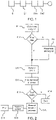
- Figure 1 illustrates an embodiment of the proposed principle.
- the recorded audio signal S1 is provided and its sample rate identified.
- the denoising processes DN1 and DN2 are configured to process recorded audio signals at specified and fixed sampling rate. Consequently, step S2 evaluates and compares the sampling rate of the recorded audio signal with the specified sampling rate. In response to a mismatch, the recorded audio signal is resampled to match the specified sampling rate. Otherwise, the recorded audio signal can be directly applied to the denoiser process.
- the term "recorded audio signal” corresponds to a recorded audio signal having a sampling rate matching a specified sampling rate of the subsequent denoising process. It should be noted that the two denoiser processes are implemented on the same sampling rate. However, this is not a requirement per se. Rather it is possible to resample the output of the first denoiser to match the sampling rate of the second denoiser process.
- the proposed method now includes two subsequent denoiser processes DN1 and DN2 arranged in a chain like structure, in which the first denoiser process DN1 acts on the recorded (and resampled) audio signal and provides it respective output to the second denoiser process DN2. It has been found that the different denoiser processes are able -in particular- in audio signals with different noise types to improve the overall denoising results. In other words, two subsequent denoiser processes arranged subsequently to each other may improve the overall audio quality and are able to compensate for an individual denoiser's drawbacks or disadvantages.
- the first of the subsequent denoiser processes DN1 is a machine-learning based denoiser process to provide a denoised spectrogram.
- the second of the two subsequent denoiser processes DN2 is implemented differently and particularly without a machine-learning based algorithm.
- the second of the two subsequent denoiser processes DN2 is a denoiser process configured to remove at least stationary noise, and optional musical noise from a spectrogram applied to it.
- FIG. 2 shows a more detailed implementation of the proposed method illustrating various aspects of the inventive concept.
- a recorded audio signal is obtained in step S1.
- the recorded audio signal may have been sampled at a certain sampling rate or the sampling rate may be unknown. Consequently, step S10 offers an evaluation, in which the sampling rate of the recorded audio signal is identified, evaluated and compared with a predetermined value.
- the predetermined value corresponds to the fixed sampling rate at which audio signals have to be applied at the denoiser process. Further, it is the sampling rate defining the generation of the spectrogram be generated from the audio signal and used for the denoising process.
- step S10 determines that the sampling rate of the recorded audio signal matches of the prespecified sampling rate, the method continues with step 11. However, if the evaluation step S10 determines that the sampling rate of the recorded audio signal does not match the specified sampling rate reassembling of the recorded audio signal will be performed in step S2 to match the specified sampling rate.
- a spectrogram is obtained by for example by performing a short time Fourier transformation, STFT on the recorded audio signal. It has been found however that for the subsequent machine-learning based denoiser process, it is a useful to extend the window length, as well as the FFT size to a large value. The improved results caused by such extension may originate from the fact that the phase of noise within the signal may be time correlated to such extent that noise may extend forwards and backwards in time. Consequently, extending the window length for the short time Fourier transformation, STFT may capture that noise completely and therefore offer better training results in the subsequent machine-learning based denoiser process.
- the obtained spectrogram comprises the amplitude and phase information for each energy or frequency bin over a certain period of time. It is applied to the first denoiser process in step S12. An implementation of the first denoiser process will be explained in greater detail below with respect to figures 3 to 5 below. Nevertheless, the first denoiser process will predict amplitude and phase information in response to its machine-learning based algorithm and provides a denoised spectrogram as an output.
- step S13 the denoised output spectrogram is evaluated with regard to quality, in order to decide whether the obtained denoising process is sufficient or second subsequent denoiser process has to be applied.
- evaluation can be done either automatically by measuring the remaining mean or median noise level or manually by simply listening to the output results by a user.
- step S14 If the evaluation determines that the quality is sufficient, the process ends step S14. If you evaluation determines that the quality is not a sufficient the output results of the first denoiser process is applied as an input to a second denoiser process in step S15.
- the second denoiser process in step S15 is implemented differently compared to the first denoiser process in step S12.
- the denoising method steps S12 and S15 are different such that in any case different results would be observed when the same audio signal is applied to them. In particular, they may apply different approaches, e.g. one denoiser if acting on the amplitude information alone, while the other denoising process utilizes phase and amplitude information to reduce the noise.
- the second denoiser process is a non-machine-learning based algorithm, with, which is configured to reduce the noise level without knowledge offer the median noise level within the spectrogram. This enables the second denoiser process to reduce the noise without knowledge of the actual noise level by sorting the various energy bins and then removing those components within the energy bins, which are smaller than a certain threshold level.
- the results of the second denoiser process is a spectrogram deprived from stationary and musical noise.
- step S16 may either perform an inverse short-term Fourier transformation ISTFT to obtain the denoised signal or alternatively perform a Griffin Lim Algorithm, GLA on the output results after the second denoiser process.
- the algorithm is a way to reconstruct of the missing part of the phase information, in case the denoising process is removing parts of the magnitude in the spectrogram. The latter may lead to inconsistencies in the phase, which can be fixed by the respective algorithm.
- the machine-learning based denoiser process makes use of two separate predicting networks P1 and P2.
- the first predicting network P1 predicts the denoised amplitude portion of the spectrogram applied to it is input while the second predicting network P2 predicts the respective phase information and outputs the denoised phase of the spectrogram.
- the phase information of the spectrogram contains almost no structure, which makes it hard for the predicting network P2 to predict correctly the denoised phase information.
- the amplitude feature map may offer a structure, which in turn may be correlated with the phase. Consequently, both networks are communicating with each other at various stages throughout the generation of the feature map.
- Each path comprises a respective input stage BP1 and BP2, at which the respective amplitude or phase information of the spectrogram is provided.
- the input of the network as a short time Fourier transformed STFT spectrogram is a complex valued spectrogram having a matrix T x F, wherein T represents of the number of times steps and F represents the number of frequency bins.
- the respective input stages comprises different groups of 2D partial convolutional layers, which are used to produce the feature map in the amplitude predicting network P1 as well as in the phase predicting network P2.
- the input stage BP1 and BP2 with their partial convolutional layers for each predicting network are coupled to a respective streaming block TSBP1 and TSBP2, respectively.
- Those streaming blocks are subsequently repeated three times for the amplitude-predicting network as well as for the phase predicting network, such that the output of each streaming block is applied to the respective input of the next streaming block.
- a cross communication link is established between the amplitude and phase predicting networks at various positions.
- the link occurs between the respective streaming blocks TSBP1 and TSBP2.
- the output of the first streaming block TSBP1 of the amplitude-predicting network P1 is combined with the output of the first streaming block TSBP2 of the phase predicting network P2 and subsequently applied is input to the next streaming block TSBP2.
- the output of the first streaming block TSBP2 of the phase predicting network is combined with the output of the first streaming block TSBP1 in the amplitude-predicting network P1 and then subsequently applied as input to the subsequent streaming block TSBP1 of the amplitude-predicting network.
- the communication between the respective amplitude and phase predicting networks take place after each of the streaming blocks TSBP1 and TSBP2, respectively.
- the exchange of information is suitable for the phase prediction as the phase itself may not comprise a significant a structure and therefore it is hard to predict.
- the outputs of the respective streaming blocks in the amplitude and phase pass of the last streaming block is then combined and subsequently applied to a respective prediction network PN1 for the amplitude and PN2 for the phase to predict the denoised amplitude and phase information.
- the input stage of the first amplitude-predicting network comprises a group of 2D partial convolutional layers CL1 and CL2, which are used to produce a respective feature map for the amplitude path.
- the partial convolutional layer CL1 include a kernel size with an n x m kernel matrix, which is followed by a subsequent convolutional layer CL2 with an m x n kernel matrix. As an example, a 1 x m matrix and its transformed counterpart an m x 1 can be used.
- the feature map output is then applied to the streaming block TSBP1.
- the stream block TSBP1 for the amplitude-predicting network comprises three convolutional layers CL3, CL4 and CL5 to handle local time frequency correlation for the input feature and the feature map provided by the input stage BP1.
- the convolutional layer comprises a different kernel sizes, whereas the total size of the first convolutional layer, CL3 and the last convolutional layer CL5 in each streaming block TSBP1 comprise the same kernel size and include a matrix of m x n.
- the convolutional layer in between includes a one-dimensional matrix of kernel size p x 1.
- the convolutional layers are surrounded by frequency transformation blocks FTB1 and FTB2 used before and after the three convolutional layers.
- the frequency transformation blocks enable the capturing of global correlation on the frequency access, such as harmonic correlations.
- the output of the last frequency transformation block of the first and second of the three streaming blocks TSBP1 is coupled to the input of the subsequent streaming block.
- the output is also combined with the output of streaming blocks TSBP2 of the phase predicting network, and vice versa.
- the combined output of the amplitude-predicting network and the phase predicting network is then subsequently applied to the next stream a block TSBP of the amplitude-predicting network and the phase predicting network, respectively.
- the phase predicting network comprises a similar structure of input stage BP2 having two partial convolutional layers of different kernel sizes.
- the input stage BP2 provides a feature map for the phase information, which is subsequently applied to the first streaming block TSBP2.
- the phase predicting network and its streaming blocks TSBP2 are simplified and only comprise two convolutional layers. It has been observed that the convolutional layers in the streaming blocks TSBP2 can comprise the same kernel structure as the partial convolutional layers in the input stage BP2 to provide the feature map. Consequently, the phase predicting network and it streaming blocks are designed lightweight.
- the second (partial) convolutional layer both in the input stage BP2, as well as in each streaming block TSBP2- comprises a kernel size m x 1 with a relatively large value for m. This enables the predicting network to capture long-range time domain correlations, which are present in the phase information.
- a global layer normalisation can be performed before each convolutional and partial convolutional layer in the phase predicting network. Further, depending on the noise characteristics, it has been found that an activation function for the phase predicting network is not necessary as the presence of such function actually decreases performance in the phase prediction.
- the communication between the amplitude-predicting network and the phase of predicting network is important to the success of the combined stream block structure.
- the phase predicting network has only a reduced success for phase prediction without additional information from the amplitude predicting network as the phase comprises no significant structure. Consequently, as shown in figure 3 , the output features of each stream block TSBP is combined before being input into the subsequent stream block or used as an input for the amplitude and phase prediction.
- the frequency transformation blocks FTB1 and FTB2 are illustrated with their main elements and structure in Figure 5 .
- the input that is the feature map either from the first input stage or the respective output from the previous stream blocks, are forwarded directly to a point-wise multiplication or fed into an attention block to predict portions of the feature map that require a higher attention.
- the attention block uses 2D and 1D convolutional layers.
- the result is subsequently multiplied with the input feature map.
- the result with the relevant feature marked by the attention map is then forwarded to element FC, which contains a trainable frequency transformation matrix that is now applied to each feature map slice for each point in time.
- each energy been in the feature map contains information from all frequency bands, allowing the subsequent correlation layers in the stream blocks to exploit global frequency correlation for amplitude and phase estimation.
- the output of the frequency transformation block FTB or FTPB2 is concatenated with the original input and then applied to a 1 ⁇ 1 convolution layer.
- normalisation and activation can be implemented for all convolution layers.
- the machine based-learning denoiser process of the proposed principle provides improved results over conventional denoising algorithms or algorithm that utilise machine-learning based. This is achieved by the phase prediction using the structure from the amplitude-predicting network taking into account that both networks are trained with audio data sampled at a higher sampling rate, e.g. in the range of 22 kHz or higher. The high sampling rate will preserve phase information even for higher harmonics of the speech fundamentals.
- partial convolution and layer, particularly as input stage provides further benefits for the respective predictions.
- the second denoiser process implements a different approach and follows the idea that a spectrogram with residual noise can further be improved without the precise knowledge of the level of stationary or musical noise.
- Figures 6 and 7 illustrate, by way of example, the various steps for the second denoiser process.
- a stationary noise often corresponds or at least is similar to arbitrary white Gaussian noise AWGN that, under usual circumstances can be directly subtracted from the audio signal.
- AWGN white Gaussian noise
- such approach requires knowledge about the overall power of the stationary noise within the audio signal to be able to calculate a medium or mean value and subsequently subtract that value from the audio signal.
- the level of noise is generally unknown and such approach usually fails.
- the inventors have proposed a revised method following the idea that the main energy portions of speech audio signal is focused on relatively few energy or frequency bins, usually around the frequency ranges for speech.
- the idea makes use of the further fact that in audio signals with a higher sampling rate the respective speech energies is concentrated in very few frequency bins.
- the pre-determined quantile instead of knowing noise in advance, it might be possible to use the pre-determined quantile on the overall spectrogram to reduce or simply remove components below the threshold given by the quantile. In other words it is assumed that energy in each time slice and frequency bin below a threshold given by the pre-determined quantile does not belong to the speech, but is noise or at least and undesired signal.
- FIG. 6 illustrates by way of examples four frequency bins f1 to f4 as well as three time slices t1 to t4 of a spectrogram. For each time slice and in each frequency bin the energy deposit in the respective tf-cell is illustrated. As visible from the left drawing, the main energy components are concentrated in relatively low frequency bins over the whole period t1 to t3. This results from the fact that for audio content having speech the main energy is concentrated in those frequency bins, in which the fundamental of the speech signal as well as first few harmonics are located. In the present case as shown in figure 6 , frequency bin f1 as well as frequency bin f2 of timeframe t3 contains the main energy portions. For evaluating the quantile and for the present example the median, the various energy components are sorted according to their energy values providing overall 12 values. Consequently, the median evaluated in this example, after the sixth value and more precisely between the values of 0.1 and 0.2.
- FIG. 6 is a right, drawing the values that are below the threshold, or simply speaking, lower than via respective medium are simply deleted and set to 0.
- the median was used.
- the quantile may be set to 0.7 or 0.8 to supress the noise.
- here is a trade-off, because for larger quantile values the risk that speech harmonics are accidently removed may increase.
- the spectrogram with already removed stationary noise is decomposed into a dense portion as well as a sparse portion.
- the dense portion mainly contains the speech information located in the lower frequency bins, while the sparse portion includes the musical noise.
- the sparse portion is removed from the overall spectrogram and an inverse short-time Fourier transformation is performed to obtain the denoised audio signal.
Landscapes
- Engineering & Computer Science (AREA)
- Computational Linguistics (AREA)
- Quality & Reliability (AREA)
- Signal Processing (AREA)
- Health & Medical Sciences (AREA)
- Audiology, Speech & Language Pathology (AREA)
- Human Computer Interaction (AREA)
- Physics & Mathematics (AREA)
- Acoustics & Sound (AREA)
- Multimedia (AREA)
- Compression, Expansion, Code Conversion, And Decoders (AREA)
Abstract
Description
- The present invention relates computer-implemented method for processing an audio signal, in particular including speech. The invention also relates to a computer system and a non-transitory computer-readable storage medium.
- Generation of high quality audio is key means for conveying a story, both for pure audio content as well as video content to a broader audience, most important for today's content providers. However, conventional audio recording methods often phase a drawback due to the mediocre or bad audio quality. While a reduced audio quality also hampers the listener's experience, another drawback lies in the fact that post processing of audio requires substantial human effort. Particularly, improving audio quality often requires several iterations, in which the content provider listens to the processed audio signal until the desired result are achieved.
- In some applications, audio is recorded in noisy environments. For example, during an outside interview the recorded audio signal may contain the speech of the interviewer and the person who is being interviewed, but also all kinds of arbitrary noise from various sources. This problem does not only occur in open environments, but also indoors, in which various other noise sources are present, thus reducing the overall quality. An important aspect for audio processing is related to a denoising process, in which the noise level of the recorded audio signal is identified and subsequently removed. This process often requires manual work and the setting of several parameters until the desired quality and best eligibility is obtained.
- Consequently, there is a desire to simplify or at least reduce the thoughts for this very time consuming task.
- The inventors have realized that audio processing and in particular speech processing requires higher sample rate to obtain all information on the recorded noise while maintaining the harmonics in the spectrogram relevant for good speech quality. When processing audio preserving of phase information seems important, as it was found that such phase information affects largely the eligibility of speech. While in conventional noise reduction solutions mainly the amplitude portion of a signal is processed thus adversely affecting the phase portion, the present application seeks to reduce noise while avoiding a distortion of the phase information in the signal, or alternatively reduce or alternatively reduce noise in the amplitude domain and reconstruct the missing phase.
- In addition, significant improvements were found when dealing with high noisy signal with a chain of two different denoisers. Such approach will reduce stationary noise, musical and high frequency noise in signals with heavy speech content. Compared to previous results, the speech signals quality can be maintained.
- Consequently, the inventors propose a computer-implemented method for processing an audio signal, in particular including speech, in which a recorded audio signal having a dedicated sampling rate, in particular above 22 kHz is obtained, the recorded audio signal comprising a speech portion and a noise portion. A spectrogram of the respective recorded audio signal is obtained. Subsequently, the obtained spectrogram is applied to a processing chain of two subsequent denoiser processes to reduce the noise in the signal. The first of the two subsequent denoiser processes is a machine-learning based denoiser process to provide a denoised spectrogram. The second of the two subsequent denoiser process is a denoiser process configured to remove at least stationary noise from a spectrogram applied to it and in particular at least one of stationary, semi-stationary, and musical noise .
- As stated previously, high quality audio content with speech require higher sampling rates. On the other hand, machine-learning based trained denoiser processes require a lot of computational power to obtain good results, and such computational effort increases significantly with higher sampling rates.
- In an aspect, the inventors therefore propose a computer-implemented method for processing an audio signal, in particular including speech. In a first step, a recorded audio signal having a sampling rate is obtained. The recorded audio signal comprising a speech portion and a noise portion. Prior to the denoiser processing it is evaluated if the sampling rate matches a specified sampling rate. Said specific sampling rate is the sampling rate, in which the machine-learning based denoiser process was trained with. In response to an evaluation that the sampling rate of the obtained recorded audio signal does not match the specified sampling rate, the recorded audio signal is resampled to match the specified sampling rate. Then a spectrogram is obtained of the recorded audio signal. The spectrogram is then applied to a machine-learning based denoiser process trained at the specified sampling rate to provide a denoised spectrogram. The machine-learning based denoiser process will separate amplitude information and phase information before applying amplitude information and phase information to a chain of partial convolutional layers, each of them having different kernel sizes.
- Consequently, the machine-learning based denoiser process will act on the amplitude and phase information separately. It was also found that amplitude and phase information should be processed initially using partial convolutional layers surprisingly causing better results after the training process compared to pure convolutional layers.
- In some aspects, the order of the denoiser processes may provide different results. Consequently, it is proposed to apply the obtained spectrogram to the first of the two subsequent denoiser processes. The output is then applied to the second of the two subsequent denoiser processes. In some instances, the output of the first denoiser process may be combined with the obtained spectrogram or portions thereof to obtain a combined spectrogram. This combined spectrogram may then be applied to the second of the two subsequent denoiser processes.
- In some aspects, a short-time Fourier transformation is performed on the recorded audio signals to obtain a spectrogram. It was found that denoising, particularly with preserving phase information requires a slightly longer time scale. Therefore to obtain the spectrogram, it is proposed to use a window length in the range of 15 ms to 75 ms, in particular 23 ms to 50 ms. Further, an optional FFT size of 1024 or 2048 is found to provide good results.
- In an aspect, the first of the two subsequent denoiser processes is the machine-learning based network structure. The network structure comprises separated prediction networks for amplitude- and phase information to provide a denoised amplitude portion and a denoised complex phase portion of the applied spectrogram. They are referred to as amplitude prediction network (that is a network for predicting amplitude information) and phase predicting network (that is a network for predicting phase information), respectively. In other words, instead of providing a trained network for the whole spectrogram or the combined information of amplitude and phase, the proposed network structure separates amplitude and phase information from the spectrogram into an amplitude portion and a phase portion and processes them separately. The reason for this approach lies in the fact that the features for the amplitude and the phase may be different. Nevertheless, it was found that a complete separation would provide deteriorated results, as phase by itself does not have a structure and will therefore be hard to estimate. In an aspect, the separated prediction networks are configured to communicate with each other. In other words, the method proposes to provide information and particularly output results from the amplitude prediction network to the phase prediction network and vice versa. With the information from the amplitude- predicting network, the features for phase estimation is significantly improved.
- In this regard, the spectrogram and more precisely the amplitude portion of the spectrogram and the phase portion of the spectrogram are each applied to a chain of two different 2D partial convolutional layers to produce a respective feature map. The layer may have all different kernel sizes. It was found that partial convolutional layer perform better at low and high frequencies, the former relevant of speech. Close to edges in the amplitude and phase portions of a time slice in the spectrogram, the result are improved, if partial convolutional filters are used instead of pure convolutional filters.
- In a further aspect, the separated prediction networks for the amplitude- and phase information comprises three subsequently arranged processing blocks including the same processing elements. Processing of information is done three times in a row, whereas the results of a processing block is input to the subsequent block. Alternatively the processing steps can also be repeatedly performed, such that the output results are feedback as inputs. The three block of the amplitude prediction network are configured to handle local time-frequency correlation of the input feature. In addition, they enable the identification of global correlations on the frequency axis such as harmonic correlations, allowing the following blocks to extract high-level features for amplitude prediction.
- As stated previously, the amplitude and phase prediction networks communicate and share information to obtain a structure for the phase prediction. For this purpose, an output of each block of the amplitude prediction network is fed into an output of the respective block of the phase prediction network. Likewise, the output of each block of the prediction network for the amplitude information is fed into the output of the respective block of the prediction network for the phase information. It should be noted that this communication loop occurs for each block in the amplitude and phase prediction networks to ensure any structure found in the amplitude features is communicated to the phase. However, it may be sufficient for some applications to reduce the communication loops and feed the output only of one block of each path the respective other path.
- In an aspect, each block of the phase prediction network comprises two subsequent convolutional layers having a kernel size equals to the kernel size of the two subsequent 2D partial convolutional layers.
- It was found that spectrogram having speech as main audio often include non-local correlations in the spectrogram along the frequency axis. A typical example is the correlations among harmonics. To capture and correctly predict those features, 2D convolution layers having small kernels may not be sufficient. Hence, it is proposed in some aspect to include a first frequency transformation block being an input element of each block of the amplitude prediction network. Likewise, a second frequency transformation block is applied to the last of each convolutional block and thus forms the output element of each block. The frequency transformation blocks each comprise a trained transformation matrix applied on the frequency axis to obtain a feature map containing information about all frequency bands. In this regard, the first and second frequency transformation block may comprise the same structure.
- After the feature map has been generated within the amplitude and phase prediction network, the respective outputs are used to predict the amplitude and phase masks. In some aspects, the amplitude prediction network comprises a bi-directional Long Short Term Memory network, Bi-LSTM with a unit number smaller than 600 for amplitude mask prediction. In addition, several fully connected layers of the same size and then a subsequently reduces size may be arranged after the Bi-LSTM network. The processed phase feature map is reduced to a complex and normalized value feature map, wherein the two channels correspond to the real and the imaginary parts of the predicted phase.
- The result combined to a spectrogram is the output of the denoising process. In some instances, the results can be transformed back using an ISTFT to obtain a denoised audio signal. In addition or alternatively a Griffin Lim Algorithm, GLA is applied to the final output of both denoiser. Applying a GLA is a possible way to reconstruct any smaller missing part of the phase, in case the second denoiser has aversively affected or removed parts of the amplitude in the spectrogram, which might lead to inconsistencies in the phase.
- In some other aspects, the spectrogram or the denoising mask from the previous denoiser may form the input of a subsequent denoising process. Hence in this regard, the subsequent denoising process may be applied to the clean denoised signal the previous denoiser or it can be given a "mask" which can be applied to give the clean signal. Further alternatively, the subsequent denoiser can receive directly the mask. Hence, the second denoiser can "denoise" the "denoising mask" of the first denoiser. In contrast to the previous one, the second denoising process uses a non-machine-learning based trained process.
- When applying the spectrogram to the second of the two subsequent denoiser process, a predetermined quantile may first be obtained out for all components of each frequency bin in the spectrogram. The quantile allows controlling how "clean" the desired output is. In some instances, a user may chose or set the quantile to some desired or pre-defined values. For example, if a recorded audio signal may still comprise an undesired noise level, a higher quantile can be chosen. In some instances the median (quantile=0.5) is selected. In a subsequent step, the selected quantile is used to remove components of the spectrogram smaller than the obtained median to provide a denoised spectrogram. This particular step make use of the fact that the human voice focusses main portions of its energy in a relatively smaller number of frequency bands Hence, higher frequency do usually not contain further speech information, apart from harmonics of the spectrum, but are usually noisy.
- Using a quantile may also have the benefit of avoiding the need of any knowledge of the actual noise level. Together with a higher sampling rate, which generates a lot of spectrogram bins, one can make use of the focussed energy in small bands and generally considers all portions below the selected quantile to be noise. As a result, the process generate a denoised spectrogram.
- In an aspect, the output of this process may then be further decomposed into a dense portion of the denoised spectrogram and a sparse portion, wherein the dense portion comprises components of the denoised spectrogram having a particular structure, and more precisely having the harmonic structure of the recorded signal.
- A different aspect is related to a computer-implemented method of any of the preceding claims, wherein the step of obtaining a recorded audio signal comprises evaluating if the sampling rate of the recorded audio signal matches a specified sampling rate. The specific sampling rate is generally higher than the usual frequency for normal speech to capture not only the fundamental frequency, but also the very high and particular all audible harmonics in the signal. The sampling rate may be therefore 44.1 kHz or multiples thereof like 98.2 kHz. Alternatively, the sampling frequency may also be 48 kHz or multiple like 96 kHz, 146 kHz 192 KHz. If the sampling rate does not match a specified sampling rate, the recorded audio signal will be resampled to match the specified sampling rate. After resampling if necessary, a spectrogram is obtained therefrom, wherein the spectrogram comprises a plurality of energy or frequency bins. The spectrogram can be obtained using ISTFT or any other suitable transformation.
- Usually the exact noise figure of the signal and the noise itself is not known in advance. The method therefore proposes to remove components of each energy bin in the spectrogram that are smaller than a previously obtained quantile to provide a first denoised spectrogram. Advantageously, the method make use of the fact that speech and language usually focusses its main portion of its energy in certain frequencies, while other frequency ranges carry relatively low energy mostly coming from noise. By proper selection of a quantile and then removing the component from the spectrogram lower than a threshold set by the quantile, one can remove the main portion of the stationary noise from the spectrogram. Depending on the desired level of noise suppression, a user may set the quantile to a dedicated value that provides him with the best results. Generally, the quantile will be higher if more noise is present in the signal.
- Any denoising method (such as the ones described above, the machine-learning-based one and a non-machine-learning based one) might lead in some instances to spurious peaks in the spectrogram which are perceived as 'musical noise'. To remove such noise, the present invention proposes to decompose the spectrogram denoising mask into a dense portion and a sparse portion, wherein the dense portion comprises components of the denoised spectrogram within a pre-determined structure, in particularly a harmonic structure.
- While this resampling as above is mentioned in respect to certain method steps, one should note that it is not restricted to a specific method. Rather re-sampling of the recorded and to-be-processed signals may be enforced as soon as the denoiser process is not set up for the sampling rate of the recorded signal. This can happen for example if the Machine-learning based denoiser has been trained with example signal of a different sampling rate. Further, the various layers and elements in the denoiser comprise a certain dimension corresponding to a certain sample rate.
- The computational effort increases with increasing sample rate significantly due to the require memory consumption and processor time needed. Hence, to obtain audio processing in a suitable time or even in real-time one has to make a trade-off between the sampling rate and the processing time. On the other hand, it has been found that processing and denoising a recorded signal at higher sampling rate usually provides better results as eligibility of the processed signal depends on correct phase reconstruction and the harmonics in the original signal.
- Another aspect concerns a computer system that comprises one or more processors. A memory is coupled to the one or more processors. The memory comprises instructions, which when executed by the one or more processors cause the one or more processors to perform the method of any of the preceding claims. A further aspect is related to non-transitory computer-readable storage medium comprising computer-executable instructions for performing the method of any of the preceding claims.
- Further aspects and embodiments in accordance with the proposed principle will become apparent in relation to the various embodiments and examples described in detail in connection with the accompanying drawings in which
-
Figure 1 shows an embodiment of the main aspects for a method of processing an audio signal in accordance with some aspects of the present invention; -
Figure 2 illustrates an exemplary embodiment of a process flow according to some aspects of the proposed principle; -
Figure 3 shows an embodiment of the prediction network in accordance with the first denoiser of the proposed principle; -
Figure 4 shows a more detailed view of potion of the amplitude prediction network in accordance with some aspects of the proposed principle; -
Figure 5 illustrates a structure of a frequency transformation block to capture global correlation in the frequency bands; -
Figure 6 and 7 show a simplified spectrogram with an energy distribution to illustrate the various proves steps of an embodiment of the second denoiser. - The following embodiments and examples disclose different aspects and their combinations according to the proposed principle. The embodiments and examples are not always to scale. Likewise, different elements can be displayed enlarged or reduced in size to emphasize individual aspects. It goes without saying that the individual aspects of the embodiments and examples shown in the figures can be combined with each other without further ado, without this contradicting the principle according to the invention. Some aspects show a regular structure or form. It should be noted that in practice slight differences and deviations from the ideal form may occur without, however, contradicting the inventive idea.
- In addition, the individual figures and aspects are not necessarily shown in the correct size, nor do the proportions between individual elements have to be essentially correct. Some aspects are highlighted by showing them enlarged. However, terms such as "above", "above" "below", "below" "larger", "smaller" and the like are correctly represented with regard to the elements in the figures. So it is possible to deduce such relations between the elements based on the figures.
- The inventors have realised that for a proper denoising process the respective audio signal should have a relatively large sampling rate to be able to reconstruct the phase information, as it turned out that the denoising process may distort the phase information of the recorded audio signal. Further, a good phase information as well as harmonics in the spectrum is helpful for the human ear to reconstruct the audio signal and provide a good eligibility. Consequently, harmonics ad phase in the recorded audio should be preserved as much as possible during the denoising process to maintain the audio quality. In addition, some content providers may perform further post processing to generate a spatial audio signal, a stereo signal or any out output.
- At the same time, a denoising process should be flexible, that is it should be able to denoiser noisy audio signal without deteriorating the quality for less noisy or clean audio signals. It has been found that current speech denoiser may not be sufficient for this purpose, as they are implemented with a relatively low sampling rate that does not allow for proper reconstruction of higher harmonics. Hence, it is proposed to provide a denoising method with a fixed sampling rate and adapt the sampling rate of recorded audio signals to be processed to the fixed sampling rate. The fixed sampling rate for the denoiser process is set to a value, which on the one side offers good results with regard to audio quality, while at the same time, only requiring foreseeable computational effort. A sampling of 48 kHz, 44 kHz has been found suitable for the denoising process according to the proposed principle. A sampling rate of 22 kHz may also be sufficient, when less computation power is available.
-
Figure 1 illustrates an embodiment of the proposed principle. The recorded audio signal S1 is provided and its sample rate identified. The denoising processes DN1 and DN2 are configured to process recorded audio signals at specified and fixed sampling rate. Consequently, step S2 evaluates and compares the sampling rate of the recorded audio signal with the specified sampling rate. In response to a mismatch, the recorded audio signal is resampled to match the specified sampling rate. Otherwise, the recorded audio signal can be directly applied to the denoiser process. - For the purpose of simplicity, the term "recorded audio signal" corresponds to a recorded audio signal having a sampling rate matching a specified sampling rate of the subsequent denoising process. It should be noted that the two denoiser processes are implemented on the same sampling rate. However, this is not a requirement per se. Rather it is possible to resample the output of the first denoiser to match the sampling rate of the second denoiser process.
- The proposed method now includes two subsequent denoiser processes DN1 and DN2 arranged in a chain like structure, in which the first denoiser process DN1 acts on the recorded (and resampled) audio signal and provides it respective output to the second denoiser process DN2. It has been found that the different denoiser processes are able -in particular- in audio signals with different noise types to improve the overall denoising results. In other words, two subsequent denoiser processes arranged subsequently to each other may improve the overall audio quality and are able to compensate for an individual denoiser's drawbacks or disadvantages.
- The first of the subsequent denoiser processes DN1 is a machine-learning based denoiser process to provide a denoised spectrogram. In contrast thereto, the second of the two subsequent denoiser processes DN2 is implemented differently and particularly without a machine-learning based algorithm. The second of the two subsequent denoiser processes DN2 is a denoiser process configured to remove at least stationary noise, and optional musical noise from a spectrogram applied to it.
- It was found by the inventors that a very noisy recorded audio signal may result in an insufficient denoised audio signal, whereas said audio signal still contains hearable and sometimes annoying noise reducing the overall audio quality. Applying the output of the first denoiser process as a machine-learning based denoiser process to second process implemented completely differently improves the overall audio quality by identifying and removing stationary and musical noise from the spectrogram.
-
Figure 2 shows a more detailed implementation of the proposed method illustrating various aspects of the inventive concept. As previously stated, a recorded audio signal is obtained in step S1. The recorded audio signal may have been sampled at a certain sampling rate or the sampling rate may be unknown. Consequently, step S10 offers an evaluation, in which the sampling rate of the recorded audio signal is identified, evaluated and compared with a predetermined value. The predetermined value corresponds to the fixed sampling rate at which audio signals have to be applied at the denoiser process. Further, it is the sampling rate defining the generation of the spectrogram be generated from the audio signal and used for the denoising process. - Consequently, if the evaluation step S10 determines that the sampling rate of the recorded audio signal matches of the prespecified sampling rate, the method continues with
step 11. However, if the evaluation step S10 determines that the sampling rate of the recorded audio signal does not match the specified sampling rate reassembling of the recorded audio signal will be performed in step S2 to match the specified sampling rate. - In step S11, a spectrogram is obtained by for example by performing a short time Fourier transformation, STFT on the recorded audio signal. It has been found however that for the subsequent machine-learning based denoiser process, it is a useful to extend the window length, as well as the FFT size to a large value. The improved results caused by such extension may originate from the fact that the phase of noise within the signal may be time correlated to such extent that noise may extend forwards and backwards in time. Consequently, extending the window length for the short time Fourier transformation, STFT may capture that noise completely and therefore offer better training results in the subsequent machine-learning based denoiser process.
- The obtained spectrogram comprises the amplitude and phase information for each energy or frequency bin over a certain period of time. It is applied to the first denoiser process in step S12. An implementation of the first denoiser process will be explained in greater detail below with respect to
figures 3 to 5 below. Nevertheless, the first denoiser process will predict amplitude and phase information in response to its machine-learning based algorithm and provides a denoised spectrogram as an output. - In step S13, the denoised output spectrogram is evaluated with regard to quality, in order to decide whether the obtained denoising process is sufficient or second subsequent denoiser process has to be applied. Such evaluation can be done either automatically by measuring the remaining mean or median noise level or manually by simply listening to the output results by a user.
- If the evaluation determines that the quality is sufficient, the process ends step S14. If you evaluation determines that the quality is not a sufficient the output results of the first denoiser process is applied as an input to a second denoiser process in step S15. The second denoiser process in step S15 is implemented differently compared to the first denoiser process in step S12. In other words, the denoising method steps S12 and S15 are different such that in any case different results would be observed when the same audio signal is applied to them. In particular, they may apply different approaches, e.g. one denoiser if acting on the amplitude information alone, while the other denoising process utilizes phase and amplitude information to reduce the noise.
- In some aspects of the second denoiser process is a non-machine-learning based algorithm, with, which is configured to reduce the noise level without knowledge offer the median noise level within the spectrogram. This enables the second denoiser process to reduce the noise without knowledge of the actual noise level by sorting the various energy bins and then removing those components within the energy bins, which are smaller than a certain threshold level. The results of the second denoiser process is a spectrogram deprived from stationary and musical noise.
- In some instances, the two denoiser processes may ultimately distort or remove components from early spectrogram. Consequently, step S16 may either perform an inverse short-term Fourier transformation ISTFT to obtain the denoised signal or alternatively perform a Griffin Lim Algorithm, GLA on the output results after the second denoiser process. The algorithm is a way to reconstruct of the missing part of the phase information, in case the denoising process is removing parts of the magnitude in the spectrogram. The latter may lead to inconsistencies in the phase, which can be fixed by the respective algorithm.
- Referring now to
Figure 3 , showing an illustration of the first denoiser process utilising a machine-learning based algorithm. The machine-learning based denoiser process makes use of two separate predicting networks P1 and P2. The first predicting network P1 predicts the denoised amplitude portion of the spectrogram applied to it is input while the second predicting network P2 predicts the respective phase information and outputs the denoised phase of the spectrogram. It has been surprisingly observed that the phase information of the spectrogram contains almost no structure, which makes it hard for the predicting network P2 to predict correctly the denoised phase information. On the other hand, the amplitude feature map may offer a structure, which in turn may be correlated with the phase. Consequently, both networks are communicating with each other at various stages throughout the generation of the feature map. - Each path comprises a respective input stage BP1 and BP2, at which the respective amplitude or phase information of the spectrogram is provided. The input of the network, as a short time Fourier transformed STFT spectrogram is a complex valued spectrogram having a matrix T x F, wherein T represents of the number of times steps and F represents the number of frequency bins. The respective input stages comprises different groups of 2D partial convolutional layers, which are used to produce the feature map in the amplitude predicting network P1 as well as in the phase predicting network P2.
- The input stage BP1 and BP2 with their partial convolutional layers for each predicting network are coupled to a respective streaming block TSBP1 and TSBP2, respectively. Those streaming blocks are subsequently repeated three times for the amplitude-predicting network as well as for the phase predicting network, such that the output of each streaming block is applied to the respective input of the next streaming block.
- In addition, as visualised in
Figure 3 , a cross communication link is established between the amplitude and phase predicting networks at various positions. The link occurs between the respective streaming blocks TSBP1 and TSBP2. Particularly, the output of the first streaming block TSBP1 of the amplitude-predicting network P1 is combined with the output of the first streaming block TSBP2 of the phase predicting network P2 and subsequently applied is input to the next streaming block TSBP2. Likewise, the output of the first streaming block TSBP2 of the phase predicting network is combined with the output of the first streaming block TSBP1 in the amplitude-predicting network P1 and then subsequently applied as input to the subsequent streaming block TSBP1 of the amplitude-predicting network. - Consequently, the communication between the respective amplitude and phase predicting networks take place after each of the streaming blocks TSBP1 and TSBP2, respectively. The exchange of information is suitable for the phase prediction as the phase itself may not comprise a significant a structure and therefore it is hard to predict. The outputs of the respective streaming blocks in the amplitude and phase pass of the last streaming block is then combined and subsequently applied to a respective prediction network PN1 for the amplitude and PN2 for the phase to predict the denoised amplitude and phase information.
- Although the general structure for the amplitude and phase pass of the predicting network in accordance with the proposed first denoiser process look similar, the respective elements within the blocks are different. Such differences are illustrated with regard to
Figure 4 , showing the block elements for the input stage BP1 and the first streaming block stage TSBP1 of the amplitude-predicting network. The input stage of the first amplitude-predicting network comprises a group of 2D partial convolutional layers CL1 and CL2, which are used to produce a respective feature map for the amplitude path. The partial convolutional layer CL1 include a kernel size with an n x m kernel matrix, which is followed by a subsequent convolutional layer CL2 with an m x n kernel matrix. As an example, a 1 x m matrix and its transformed counterpart anm x 1 can be used. The feature map output is then applied to the streaming block TSBP1. - The stream block TSBP1 for the amplitude-predicting network comprises three convolutional layers CL3, CL4 and CL5 to handle local time frequency correlation for the input feature and the feature map provided by the input stage BP1.
- The convolutional layer comprises a different kernel sizes, whereas the total size of the first convolutional layer, CL3 and the last convolutional layer CL5 in each streaming block TSBP1 comprise the same kernel size and include a matrix of m x n. The convolutional layer in between includes a one-dimensional matrix of
kernel size p x 1. The convolutional layers are surrounded by frequency transformation blocks FTB1 and FTB2 used before and after the three convolutional layers. The frequency transformation blocks enable the capturing of global correlation on the frequency access, such as harmonic correlations. The output of the last frequency transformation block of the first and second of the three streaming blocks TSBP1 is coupled to the input of the subsequent streaming block. - In addition, as illustrated in
Figure 3 , the output is also combined with the output of streaming blocks TSBP2 of the phase predicting network, and vice versa. As a result, the combined output of the amplitude-predicting network and the phase predicting network is then subsequently applied to the next stream a block TSBP of the amplitude-predicting network and the phase predicting network, respectively. - The phase predicting network comprises a similar structure of input stage BP2 having two partial convolutional layers of different kernel sizes. The input stage BP2 provides a feature map for the phase information, which is subsequently applied to the first streaming block TSBP2. However, in contrast to the amplitude-predicting network, the phase predicting network and its streaming blocks TSBP2 are simplified and only comprise two convolutional layers. It has been observed that the convolutional layers in the streaming blocks TSBP2 can comprise the same kernel structure as the partial convolutional layers in the input stage BP2 to provide the feature map. Consequently, the phase predicting network and it streaming blocks are designed lightweight. In the present implementation of the phase predicting network, the second (partial) convolutional layer -both in the input stage BP2, as well as in each streaming block TSBP2- comprises a
kernel size m x 1 with a relatively large value for m. This enables the predicting network to capture long-range time domain correlations, which are present in the phase information. - In some instances, a global layer normalisation can be performed before each convolutional and partial convolutional layer in the phase predicting network. Further, depending on the noise characteristics, it has been found that an activation function for the phase predicting network is not necessary as the presence of such function actually decreases performance in the phase prediction.
- As stated previously, the communication between the amplitude-predicting network and the phase of predicting network is important to the success of the combined stream block structure. Particularly, the phase predicting network has only a reduced success for phase prediction without additional information from the amplitude predicting network as the phase comprises no significant structure. Consequently, as shown in
figure 3 , the output features of each stream block TSBP is combined before being input into the subsequent stream block or used as an input for the amplitude and phase prediction. The functional block f(TSPBl, TSBP2), using a gating mechanism for combination, is similar in both networks and includes an element of element-wise multiplication of the output of a streaming block the respective predicting network with a 1×1 convolution of the respective output of the other streaming block: f(TSPB1, TSBP2)= TSPB1 o CL(TSBP2) with CL being the 1×1 convolution. - The frequency transformation blocks FTB1 and FTB2 are illustrated with their main elements and structure in
Figure 5 . The input that is the feature map either from the first input stage or the respective output from the previous stream blocks, are forwarded directly to a point-wise multiplication or fed into an attention block to predict portions of the feature map that require a higher attention. The attention block uses 2D and 1D convolutional layers. The result is subsequently multiplied with the input feature map. The result with the relevant feature marked by the attention map is then forwarded to element FC, which contains a trainable frequency transformation matrix that is now applied to each feature map slice for each point in time. - After this block each energy been in the feature map contains information from all frequency bands, allowing the subsequent correlation layers in the stream blocks to exploit global frequency correlation for amplitude and phase estimation. The output of the frequency transformation block FTB or FTPB2 is concatenated with the original input and then applied to a 1×1 convolution layer. In addition, normalisation and activation can be implemented for all convolution layers.
- The machine based-learning denoiser process of the proposed principle provides improved results over conventional denoising algorithms or algorithm that utilise machine-learning based. This is achieved by the phase prediction using the structure from the amplitude-predicting network taking into account that both networks are trained with audio data sampled at a higher sampling rate, e.g. in the range of 22 kHz or higher. The high sampling rate will preserve phase information even for higher harmonics of the speech fundamentals. In addition, it was found that partial convolution and layer, particularly as input stage provides further benefits for the respective predictions.
- The second denoiser process implements a different approach and follows the idea that a spectrogram with residual noise can further be improved without the precise knowledge of the level of stationary or musical noise.
Figures 6 and 7 illustrate, by way of example, the various steps for the second denoiser process. In this regard, it is assumed that a stationary noise often corresponds or at least is similar to arbitrary white Gaussian noise AWGN that, under usual circumstances can be directly subtracted from the audio signal. However, such approach requires knowledge about the overall power of the stationary noise within the audio signal to be able to calculate a medium or mean value and subsequently subtract that value from the audio signal. In certain applications, for example with denoising in real-time, but also for recorded audio signals the level of noise is generally unknown and such approach usually fails. - Consequently, the inventors have proposed a revised method following the idea that the main energy portions of speech audio signal is focused on relatively few energy or frequency bins, usually around the frequency ranges for speech. The idea makes use of the further fact that in audio signals with a higher sampling rate the respective speech energies is concentrated in very few frequency bins. Hence, instead of knowing noise in advance, it might be possible to use the pre-determined quantile on the overall spectrogram to reduce or simply remove components below the threshold given by the quantile. In other words it is assumed that energy in each time slice and frequency bin below a threshold given by the pre-determined quantile does not belong to the speech, but is noise or at least and undesired signal.
- Such approach is presented in
Figure 6 in the left and right drawings. The left drawing illustrates by way of examples four frequency bins f1 to f4 as well as three time slices t1 to t4 of a spectrogram. For each time slice and in each frequency bin the energy deposit in the respective tf-cell is illustrated. As visible from the left drawing, the main energy components are concentrated in relatively low frequency bins over the whole period t1 to t3. This results from the fact that for audio content having speech the main energy is concentrated in those frequency bins, in which the fundamental of the speech signal as well as first few harmonics are located. In the present case as shown infigure 6 , frequency bin f1 as well as frequency bin f2 of timeframe t3 contains the main energy portions. For evaluating the quantile and for the present example the median, the various energy components are sorted according to their energy values providing overall 12 values. Consequently, the median evaluated in this example, after the sixth value and more precisely between the values of 0.1 and 0.2. - In accordance with the present invention shown in
Figure 6 is a right, drawing the values that are below the threshold, or simply speaking, lower than via respective medium are simply deleted and set to 0. For this example, the median was used. However, one may use a lower or higher quantile depending on the noise level. For very noisy signals, the quantile may be set to 0.7 or 0.8 to supress the noise. However, here is a trade-off, because for larger quantile values the risk that speech harmonics are accidently removed may increase. - This process step will result in the structure showing in
figure 7 , left drawing, in which several values have been set to 0, except for the main speech components in frequency bin f1 and f2. This approach will already remove most of stationary noise but -as shown inFigure 7 - leave out several residual components, here in frequency bin f3 for time t1 and frequency bin f4 for time t2. These residual components are considered musical noise, as they do not relate to the speech itself, but most likely originate from spurious leftovers. - In the next step, according to the proposed principle, the spectrogram with already removed stationary noise is decomposed into a dense portion as well as a sparse portion. The dense portion mainly contains the speech information located in the lower frequency bins, while the sparse portion includes the musical noise. After the decomposition, the sparse portion is removed from the overall spectrogram and an inverse short-time Fourier transformation is performed to obtain the denoised audio signal.
Claims (17)
- A computer-implemented method for processing an audio signal, in particular including speech, comprising the steps of:- obtaining a recorded audio signal having a dedicated sampling rate, in particular above 22 kHz, the recorded audio signal comprising a speech portion and a noise portion;- obtaining a spectrogram of the recorded audio signal;- applying the spectrogram to a processing chain of two subsequent denoiser processes,wherein a first of the two subsequent denoiser processes is a machine-learning based denoiser process to provide a denoised spectrogram;
wherein the second of the two subsequent denoiser process is a denoiser process configured to remove at least stationary noise from a spectrogram applied to it. - A computer-implemented method for processing an audio signal, in particular including speech, comprising the steps of:- obtaining a recorded audio signal having a sampling rate, the recorded audio signal comprising a speech portion and a noise portion;- evaluating if the sampling rate matches a specified sampling rate;- in response to an evaluation that the sampling rate does not match the specified sampling rate:
Resampling the recorded audio signal to match the specified sampling rate;- obtaining a spectrogram of the recorded audio signal;- applying the spectrogram to a machine-learning based denoiser process trained at the specified sampling rate to provide a denoised spectrogram;wherein the machine-learning based denoiser process separates amplitude information and phase information before applying amplitude information and phase information to a chain of partial convolutional layers, each of them having different kernel sizes. - The computer-implemented method according to claim 1, wherein the obtained spectrogram is applied to the first of the two subsequent denoiser processes and its output is applied as a combined spectrogram to the second of the two subsequent denoiser processes.
- The computer-implemented method according to any of the preceding claims, wherein the step of obtaining a spectrogram comprising one of the steps of:- obtaining a STFT from the recorded audio signal with a window length in the range of 15 ms to 75 ms, in particular 23 ms to 50 ms and an optional FFT size of 1024 or 2048.
- The computer-implemented method according to any of the preceding claims, wherein the first of the two subsequent denoiser processes comprises a network for predicting amplitude information and a network for predicting phase information separated from the network for prediction amplitude information to provide a denoised amplitude portion and a denoised complex phase portion of the applied spectrogram, whereas the separated networks are configured to communicate with each other.
- The computer-implemented method according to claim 4, wherein for each separated prediction network, the applied spectrogram is input to chain of two subsequent 2D partial convolutional layers to produce a respective feature map.
- The computer-implemented method according to claim 5 or 6, wherein the separated prediction networks for the amplitude- and phase information comprises three subsequently arranged blocks including the same processing elements.
- The computer-implemented method according to claim 7, wherein an output of each block of the prediction network for the amplitude information is fed into an output of the respective block of the prediction network for the phase information;
and the output of each block of the prediction network for the amplitude information is fed into the output of the respective block of the prediction network for the phase information. - The computer-implemented method according to any of claims 6 to 8, wherein each block of the prediction network for the phase information comprises two subsequent convolutional layers having the same kernel size as the two subsequent 2D partial convolutional layers.
- The computer-implemented method according to any of claims 6 to 9, wherein each block of the prediction network for the amplitude information comprises a first frequency transformation block being the input element of each block and a second frequency transformation block being the output element of each block, the frequency transformation block comprising a trained transformation matrix to obtain a feature map containing information about all frequency bands.
- The computer-implemented method according to any of claims 5 to 10, wherein the prediction network for the amplitude information comprises a bi-directional Long Short Term Memory network, Bi-LSTM with a unit number smaller than 600.
- The computer-implemented method of any of the preceding claims, wherein applying the spectrogram to the second of the two subsequent denoiser process comprises:- obtaining a predetermined quantile, in particular the median out of all components of each frequency bin in the spectrogram;- removing components of the spectrogram smaller than the obtained median to provide a denoised spectrogram;
- The computer-implemented method of claim 12, further comprising:- decomposing the denoised spectrogram into a dense portion and a sparse portion, wherein the dense portion comprises components of the denoised spectrogram, that comprise in particular a harmonic structure.
- The computer-implemented method of any of the preceding claims, wherein the step of obtaining a recorded audio signal comprises:- evaluating if the sampling rate of the recorded audio signal matches a specified sampling rate, the specific sampling rate being one of:- 44.1 kHz or multiples thereof- 48 kHz or multiples thereof;- in response to an evaluation that the sampling rate does not match the specified sampling rate:
Resampling the recorded audio signal to match the specified sampling rate; - A computer-implemented method for processing an audio signal, in particular including speech, comprising the steps of:- obtaining a recorded audio signal having a sampling rate, the recorded audio signal comprising a speech portion and a noise portion;- evaluating if the sampling rate matches a specified sampling rate;- in response to an evaluation that the sampling rate does not match the specified sampling rate:
Resampling the recorded audio signal to match the specified sampling rate;- obtaining a spectrogram of the recorded audio signal, wherein the spectrogram comprises a plurality of frequency bins;- obtaining a predetermined quantile, in particular the median out of all components of each frequency bin in the spectrogram;- removing components of each frequency bin in the spectrogram smaller than the obtained the predetermined quantile to provide a first denoised spectrogram;- decomposing the denoised spectrogram into a dense portion and a sparse portion, wherein the dense portion comprises components of the denoised spectrogram within a pre-determined structure, in particularly a harmonic structure. - A computer system comprising:- one or more processors;- a memory coupled to the one or more processors and comprising instructions, which when executed by the one or more processors cause the one or more processors to perform the method of any of the preceding claims.
- A non-transitory computer-readable storage medium comprising computer-executable instructions for performing the method of any of the preceding claims.
Priority Applications (1)
| Application Number | Priority Date | Filing Date | Title |
|---|---|---|---|
| EP21177856.8A EP4099324B1 (en) | 2021-06-04 | 2021-06-04 | Methods for processing an audio signal and computer system |
Applications Claiming Priority (1)
| Application Number | Priority Date | Filing Date | Title |
|---|---|---|---|
| EP21177856.8A EP4099324B1 (en) | 2021-06-04 | 2021-06-04 | Methods for processing an audio signal and computer system |
Publications (3)
| Publication Number | Publication Date |
|---|---|
| EP4099324A1 true EP4099324A1 (en) | 2022-12-07 |
| EP4099324C0 EP4099324C0 (en) | 2025-12-10 |
| EP4099324B1 EP4099324B1 (en) | 2025-12-10 |
Family
ID=76283668
Family Applications (1)
| Application Number | Title | Priority Date | Filing Date |
|---|---|---|---|
| EP21177856.8A Active EP4099324B1 (en) | 2021-06-04 | 2021-06-04 | Methods for processing an audio signal and computer system |
Country Status (1)
| Country | Link |
|---|---|
| EP (1) | EP4099324B1 (en) |
Cited By (1)
| Publication number | Priority date | Publication date | Assignee | Title |
|---|---|---|---|---|
| WO2025209070A1 (en) * | 2024-04-03 | 2025-10-09 | 钉钉(中国)信息技术有限公司 | Audio processing method, audio processing model training method, and device, storage medium and program product |
Family Cites Families (1)
| Publication number | Priority date | Publication date | Assignee | Title |
|---|---|---|---|---|
| US7383179B2 (en) * | 2004-09-28 | 2008-06-03 | Clarity Technologies, Inc. | Method of cascading noise reduction algorithms to avoid speech distortion |
-
2021
- 2021-06-04 EP EP21177856.8A patent/EP4099324B1/en active Active
Non-Patent Citations (3)
| Title |
|---|
| DACHENG YIN ET AL: "PHASEN: A Phase-and-Harmonics-Aware Speech Enhancement Network", ARXIV.ORG, CORNELL UNIVERSITY LIBRARY, 201 OLIN LIBRARY CORNELL UNIVERSITY ITHACA, NY 14853, 12 November 2019 (2019-11-12), XP081530691 * |
| LI ANDONG ET AL: "Two Heads are Better Than One: A Two-Stage Complex Spectral Mapping Approach for Monaural Speech Enhancement", IEEE/ACM TRANSACTIONS ON AUDIO, SPEECH, AND LANGUAGE PROCESSING, IEEE, USA, vol. 29, 14 May 2021 (2021-05-14), pages 1829 - 1843, XP011858877, ISSN: 2329-9290, [retrieved on 20210608], DOI: 10.1109/TASLP.2021.3079813 * |
| SADASIVAN JISHNU ET AL: "Musical noise suppression using a low-rank and sparse matrix decomposition approach", SPEECH COMMUNICATION, ELSEVIER SCIENCE PUBLISHERS , AMSTERDAM, NL, vol. 125, 21 September 2020 (2020-09-21), pages 41 - 52, XP086398002, ISSN: 0167-6393, [retrieved on 20200921], DOI: 10.1016/J.SPECOM.2020.09.001 * |
Cited By (1)
| Publication number | Priority date | Publication date | Assignee | Title |
|---|---|---|---|---|
| WO2025209070A1 (en) * | 2024-04-03 | 2025-10-09 | 钉钉(中国)信息技术有限公司 | Audio processing method, audio processing model training method, and device, storage medium and program product |
Also Published As
| Publication number | Publication date |
|---|---|
| EP4099324C0 (en) | 2025-12-10 |
| EP4099324B1 (en) | 2025-12-10 |
Similar Documents
| Publication | Publication Date | Title |
|---|---|---|
| CN109686381B (en) | Signal processors and related methods for signal enhancement | |
| EP3899936B1 (en) | Source separation using an estimation and control of sound quality | |
| US7243060B2 (en) | Single channel sound separation | |
| Madhu et al. | The potential for speech intelligibility improvement using the ideal binary mask and the ideal wiener filter in single channel noise reduction systems: Application to auditory prostheses | |
| US20030014248A1 (en) | Method and system for enhancing speech in a noisy environment | |
| Gerkmann et al. | Spectral masking and filtering | |
| US10109290B2 (en) | Multi-band noise reduction system and methodology for digital audio signals | |
| Wu et al. | Subband Kalman filtering for speech enhancement | |
| WO2011137258A1 (en) | Multi-microphone robust noise suppression | |
| Garg | Speech enhancement using long short term memory with trained speech features and adaptive wiener filter | |
| JPH07248793A (en) | NOISE SUPPRESSED VOICE ANALYZER, NOISE SUPPRESSED SPEECH SYNTHESIS DEVICE, AND VOICE TRANSMISSION SYSTEM | |
| EP4099324B1 (en) | Methods for processing an audio signal and computer system | |
| EP4531042A1 (en) | Noise reduction system for dynamic noise reduction | |
| Hidri et al. | About multichannel speech signal extraction and separation techniques | |
| KR20030031660A (en) | Apparatus and method for computing speech absence probability, apparatus and method for removing noise using the computation appratus and method | |
| Zhan et al. | DeepPEM-AFC: An improved prediction-error-method-based adaptive feedback cancellation with deep learning for hearing aids | |
| Saleem | Single channel noise reduction system in low SNR | |
| US20190348060A1 (en) | Apparatus and method for enhancing a wanted component in a signal | |
| Park et al. | Postprocessing with Wiener filtering technique for reducing residual crosstalk in blind source separation | |
| Manikandan | Speech enhancement based on wavelet denoising | |
| Saoud et al. | New speech enhancement based on discrete orthonormal stockwell transform | |
| Li et al. | Improving speech enhancement by cross-and sub-band processing with state space model | |
| KR20190037867A (en) | Device, method and computer program for removing noise from noisy speech data | |
| Hoya et al. | Stereophonic noise reduction using a combined sliding subspace projection and adaptive signal enhancement | |
| Childers et al. | Co--Channel speech separation |
Legal Events
| Date | Code | Title | Description |
|---|---|---|---|
| PUAI | Public reference made under article 153(3) epc to a published international application that has entered the european phase |
Free format text: ORIGINAL CODE: 0009012 |
|
| STAA | Information on the status of an ep patent application or granted ep patent |
Free format text: STATUS: THE APPLICATION HAS BEEN PUBLISHED |
|
| AK | Designated contracting states |
Kind code of ref document: A1 Designated state(s): AL AT BE BG CH CY CZ DE DK EE ES FI FR GB GR HR HU IE IS IT LI LT LU LV MC MK MT NL NO PL PT RO RS SE SI SK SM TR |
|
| STAA | Information on the status of an ep patent application or granted ep patent |
Free format text: STATUS: REQUEST FOR EXAMINATION WAS MADE |
|
| 17P | Request for examination filed |
Effective date: 20230606 |
|
| RBV | Designated contracting states (corrected) |
Designated state(s): AL AT BE BG CH CY CZ DE DK EE ES FI FR GB GR HR HU IE IS IT LI LT LU LV MC MK MT NL NO PL PT RO RS SE SI SK SM TR |
|
| STAA | Information on the status of an ep patent application or granted ep patent |
Free format text: STATUS: EXAMINATION IS IN PROGRESS |
|
| 17Q | First examination report despatched |
Effective date: 20231130 |
|
| RAP3 | Party data changed (applicant data changed or rights of an application transferred) |
Owner name: NOMONO AS |
|
| GRAP | Despatch of communication of intention to grant a patent |
Free format text: ORIGINAL CODE: EPIDOSNIGR1 |
|
| STAA | Information on the status of an ep patent application or granted ep patent |
Free format text: STATUS: GRANT OF PATENT IS INTENDED |
|
| INTG | Intention to grant announced |
Effective date: 20250714 |
|
| GRAS | Grant fee paid |
Free format text: ORIGINAL CODE: EPIDOSNIGR3 |
|
| GRAA | (expected) grant |
Free format text: ORIGINAL CODE: 0009210 |
|
| STAA | Information on the status of an ep patent application or granted ep patent |
Free format text: STATUS: THE PATENT HAS BEEN GRANTED |
|
| AK | Designated contracting states |
Kind code of ref document: B1 Designated state(s): AL AT BE BG CH CY CZ DE DK EE ES FI FR GB GR HR HU IE IS IT LI LT LU LV MC MK MT NL NO PL PT RO RS SE SI SK SM TR |
|
| REG | Reference to a national code |
Ref country code: CH Ref legal event code: F10 Free format text: ST27 STATUS EVENT CODE: U-0-0-F10-F00 (AS PROVIDED BY THE NATIONAL OFFICE) Effective date: 20251210 Ref country code: GB Ref legal event code: FG4D |
|
| REG | Reference to a national code |
Ref country code: DE Ref legal event code: R096 Ref document number: 602021043983 Country of ref document: DE |
|
| REG | Reference to a national code |
Ref country code: IE Ref legal event code: FG4D |
|
| U01 | Request for unitary effect filed |
Effective date: 20260109 |
|
| U07 | Unitary effect registered |
Designated state(s): AT BE BG DE DK EE FI FR IT LT LU LV MT NL PT RO SE SI Effective date: 20260116 |
|
| REG | Reference to a national code |
Ref country code: CH Ref legal event code: R17 Free format text: ST27 STATUS EVENT CODE: U-0-0-R10-R17 (AS PROVIDED BY THE NATIONAL OFFICE) Effective date: 20260227 |
|
| PG25 | Lapsed in a contracting state [announced via postgrant information from national office to epo] |
Ref country code: ES Free format text: LAPSE BECAUSE OF FAILURE TO SUBMIT A TRANSLATION OF THE DESCRIPTION OR TO PAY THE FEE WITHIN THE PRESCRIBED TIME-LIMIT Effective date: 20251210 |
|
| PG25 | Lapsed in a contracting state [announced via postgrant information from national office to epo] |
Ref country code: HR Free format text: LAPSE BECAUSE OF FAILURE TO SUBMIT A TRANSLATION OF THE DESCRIPTION OR TO PAY THE FEE WITHIN THE PRESCRIBED TIME-LIMIT Effective date: 20251210 |
|
| PG25 | Lapsed in a contracting state [announced via postgrant information from national office to epo] |
Ref country code: RS Free format text: LAPSE BECAUSE OF FAILURE TO SUBMIT A TRANSLATION OF THE DESCRIPTION OR TO PAY THE FEE WITHIN THE PRESCRIBED TIME-LIMIT Effective date: 20260310 |