EP3926507A1 - Helicopter rotor airfoil determination method and system - Google Patents
Helicopter rotor airfoil determination method and system Download PDFInfo
- Publication number
- EP3926507A1 EP3926507A1 EP20879600.3A EP20879600A EP3926507A1 EP 3926507 A1 EP3926507 A1 EP 3926507A1 EP 20879600 A EP20879600 A EP 20879600A EP 3926507 A1 EP3926507 A1 EP 3926507A1
- Authority
- EP
- European Patent Office
- Prior art keywords
- airfoil
- coefficient
- generation
- mapping relationship
- population
- Prior art date
- Legal status (The legal status is an assumption and is not a legal conclusion. Google has not performed a legal analysis and makes no representation as to the accuracy of the status listed.)
- Withdrawn
Links
Images


Classifications
-
- G—PHYSICS
- G06—COMPUTING OR CALCULATING; COUNTING
- G06N—COMPUTING ARRANGEMENTS BASED ON SPECIFIC COMPUTATIONAL MODELS
- G06N3/00—Computing arrangements based on biological models
- G06N3/12—Computing arrangements based on biological models using genetic models
- G06N3/126—Evolutionary algorithms, e.g. genetic algorithms or genetic programming
-
- B—PERFORMING OPERATIONS; TRANSPORTING
- B64—AIRCRAFT; AVIATION; COSMONAUTICS
- B64C—AEROPLANES; HELICOPTERS
- B64C27/00—Rotorcraft; Rotors peculiar thereto
- B64C27/32—Rotors
- B64C27/46—Blades
- B64C27/467—Aerodynamic features
-
- B—PERFORMING OPERATIONS; TRANSPORTING
- B64—AIRCRAFT; AVIATION; COSMONAUTICS
- B64F—GROUND OR AIRCRAFT-CARRIER-DECK INSTALLATIONS SPECIALLY ADAPTED FOR USE IN CONNECTION WITH AIRCRAFT; DESIGNING, MANUFACTURING, ASSEMBLING, CLEANING, MAINTAINING OR REPAIRING AIRCRAFT, NOT OTHERWISE PROVIDED FOR; HANDLING, TRANSPORTING, TESTING OR INSPECTING AIRCRAFT COMPONENTS, NOT OTHERWISE PROVIDED FOR
- B64F5/00—Designing, manufacturing, assembling, cleaning, maintaining or repairing aircraft, not otherwise provided for; Handling, transporting, testing or inspecting aircraft components, not otherwise provided for
-
- G—PHYSICS
- G06—COMPUTING OR CALCULATING; COUNTING
- G06F—ELECTRIC DIGITAL DATA PROCESSING
- G06F18/00—Pattern recognition
- G06F18/20—Analysing
- G06F18/21—Design or setup of recognition systems or techniques; Extraction of features in feature space; Blind source separation
- G06F18/214—Generating training patterns; Bootstrap methods, e.g. bagging or boosting
-
- G—PHYSICS
- G06—COMPUTING OR CALCULATING; COUNTING
- G06F—ELECTRIC DIGITAL DATA PROCESSING
- G06F30/00—Computer-aided design [CAD]
- G06F30/10—Geometric CAD
- G06F30/15—Vehicle, aircraft or watercraft design
-
- G—PHYSICS
- G06—COMPUTING OR CALCULATING; COUNTING
- G06F—ELECTRIC DIGITAL DATA PROCESSING
- G06F30/00—Computer-aided design [CAD]
- G06F30/20—Design optimisation, verification or simulation
- G06F30/28—Design optimisation, verification or simulation using fluid dynamics, e.g. using Navier-Stokes equations or computational fluid dynamics [CFD]
-
- G—PHYSICS
- G06—COMPUTING OR CALCULATING; COUNTING
- G06F—ELECTRIC DIGITAL DATA PROCESSING
- G06F2111/00—Details relating to CAD techniques
- G06F2111/06—Multi-objective optimisation, e.g. Pareto optimisation using simulated annealing [SA], ant colony algorithms or genetic algorithms [GA]
-
- G—PHYSICS
- G06—COMPUTING OR CALCULATING; COUNTING
- G06F—ELECTRIC DIGITAL DATA PROCESSING
- G06F2111/00—Details relating to CAD techniques
- G06F2111/10—Numerical modelling
-
- G—PHYSICS
- G06—COMPUTING OR CALCULATING; COUNTING
- G06F—ELECTRIC DIGITAL DATA PROCESSING
- G06F2113/00—Details relating to the application field
- G06F2113/08—Fluids
-
- G—PHYSICS
- G06—COMPUTING OR CALCULATING; COUNTING
- G06F—ELECTRIC DIGITAL DATA PROCESSING
- G06F2119/00—Details relating to the type or aim of the analysis or the optimisation
- G06F2119/14—Force analysis or force optimisation, e.g. static or dynamic forces
-
- G—PHYSICS
- G06—COMPUTING OR CALCULATING; COUNTING
- G06N—COMPUTING ARRANGEMENTS BASED ON SPECIFIC COMPUTATIONAL MODELS
- G06N5/00—Computing arrangements using knowledge-based models
- G06N5/01—Dynamic search techniques; Heuristics; Dynamic trees; Branch-and-bound
Definitions
- the present disclosure relates to the technical field of rotor airfoil design, and in particular, to a method and system for determining a helicopter rotor airfoil.
- a rotor is a key lift and control component of a helicopter. Aerodynamic characteristics of an airfoil have important influence on aerodynamic performance and control characteristics of the rotor and the helicopter. When the helicopter flies forward, rotor blades perform rotation, flapping, and pitching simultaneously. In this way, blade sections are under periodically changing incoming flows and angles of attack, and dynamic stall may occur on a trailing side, resulting in a sharp drop in lift and a sudden increase in drag and moments. This is not conducive to flight. Therefore, reducing or even avoiding the occurrence of dynamic airfoil stall in a rotor environment plays an important role in improving the aerodynamic performance and control performance of the rotor.
- the present disclosure provides the method and system for determining a helicopter rotor airfoil.
- An optimization method for determining dynamic characteristics of the airfoil in the condition with the changing incoming flow and the changing angle of attack is constructed based on the CST method, the LHS method, the CFD method, and a multi-objective genetic algorithm NSGA-II.
- An optimized airfoil determined by using the method or the system can effectively suppress a leading edge vortex of the airfoil in the condition with the changing incoming flow and the changing angle of attack, so that lift, drag, and moments of the airfoil are not affected when the leading edge vortex moves on or falls off a surface of the airfoil, thereby avoiding a sharp drop in the lift and divergence of the drag and the moment, and greatly improving dynamic aerodynamic characteristics of the airfoil.
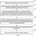
- a method for determining a helicopter rotor airfoil in an embodiment includes the following steps.
- Step S1 Randomly generate a sample point by using an LHS method.
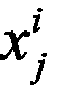
- the step S1 is specifically: generating a sample point x j i by using the LHS method, where j represents a number of the sample point, and i represents a number of a variable. It is assumed that m samples are to be extracted from n -dimensional vector space.
- LHS includes the following steps: (1) dividing each dimension into m non-overlapping intervals, so that all the intervals have a same probability; (2) randomly extracting a point from each interval of each dimension; and (3) extracting, from each dimension, the point selected in the step (2), to constitute a vector.
- Step S2 Determine characterization equations of upper and lower airfoil surfaces of an airfoil based on the sample point by using a CST method.
- the CST method is used to fit a baseline airfoil and generate an airfoil in sample space.
- ⁇ u represents a dimensionless vertical coordinate of a point on the upper airfoil surface of the airfoil
- ⁇ l represents a dimensionless vertical coordinate of a point on the lower airfoil surface of the airfoil
- y u represents a vertical coordinate of the point on the upper airfoil surface of the airfoil
- y l represents a vertical coordinate of the point on the lower airfoil surface of the airfoil
- a a number of a polynomial
- b an order of the polynomial
- a 0,1,..., b .
- Different geometric profiles of the airfoil can be obtained by adjusting values of the coefficients A u k and A l k . Therefore, the coefficients A u k and A l k are used as design variables for optimization design of the airfoil, and are optimized to obtain an optimized airfoil profile satisfying a requirement.
- a six-order Bernstein polynomial is used as the shape function.
- a coefficient of the polynomial is a design variable, and is optimized to obtain a new optimized airfoil.
- the baseline airfoil namely, an SC1095 airfoil
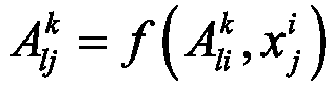
- the sample point generated by the LHS method is used to obtain polynomial coefficients of a sample airfoil numbered j (the j th sample point x j i ):
- a uj k ⁇ A ui k x j i and
- a lj k ⁇ A li k x j i , where i represents the number of the variable, and ⁇ ( ⁇ ) represents a transformation function.
- the foregoing polynomial coefficients are substituted into the characterization equations of the upper and lower airfoil surfaces of the airfoil to obtain coordinates of all sample points.
- Step S3 Perform dynamic characteristic simulation on the airfoil according to the characterization equations of the upper and lower airfoil surfaces by using a CFD method, to obtain a flow field characteristic of the airfoil, where the flow field characteristic includes a lift coefficient, a drag coefficient, and a moment coefficient.
- the CFD method is used to perform dynamic characteristic simulation on the airfoil in the sample space.
- the flow field characteristic of the airfoil is calculated based on the solution of the fluid control equation.
- Step S4 Establish a mapping relationship between the sample point and the flow field characteristic by using a Kriging model, and train the mapping relationship by using a maximum likelihood estimation method and an EI criterion, to obtain a trained mapping relationship.
- the step S4 specifically includes the following substeps.
- ns represents a quantity of the sample points
- f ⁇ 1 x ⁇ ⁇ p x
- F ⁇ 1 x 1 ... ⁇ p x 1 ⁇ ⁇ ⁇ ⁇ 1 x ns ⁇ ⁇ p x ns , ⁇ 1 ( ⁇ ),..., ⁇ p ( ⁇ ) represents a known polynomial function
- the EI criterion is used to find a new sample point with a maximum value of a mathematical expectation and a new sample point with an optimal objective function value in a process of training the Kriging model, and the two new sample points are used for training optimization of the model, till a convergence condition is satisfied.
- ⁇ l (x) is used as an example, and ⁇ d (x) and ⁇ m (x) are similar to ⁇ l (x) .
- ⁇ l (x) of any prediction point x is characterized by normal random distribution, in other words, satisfies ⁇ l (x)- -N ( ⁇ ,s 2 ), where ⁇ represents an average predicted value, and s represents a standard deviation.
- ⁇ l min represents a minimum value of the sample point
- ⁇ represents a standard normal distribution function
- ⁇ represents a density function of normal distribution.
- an optimal improved point x can always be found.
- a specific process is as follows: (1) Substitute x into a CST formula to generate a new airfoil. (2) Generate a grid. (3) Calculate dynamic characteristics. (4) Add related data of the airfoil to the sample airfoil space, to re-establish the Kriging model. (5) Train the Kriging model by using the EI criterion, to obtain the optimal improved point x. Repeat the steps (1) to (5) till prediction precision of a surrogate model satisfies a requirement, so that the mapping relationship between x j i , and Cl,Cd,Cm is established.
- Step S5 Determine an optimal sample point based on the trained mapping relationship by using NSGA-II.
- the optimal sample point corresponds to an optimal flow field characteristic, and the optimal flow field characteristic includes an optimal lift coefficient, an optimal drag coefficient, and an optimal moment coefficient.
- the step S5 specifically includes the following substeps:
- a specific process of finding an optimal airfoil by using NSGA-II is as follows: (1) Randomly generate an initial population x 1 , x 2 ,..., x N whose scale is N. (2) Calculate Cl,Cd,Cm of each individual in the population by using the mapping relationship established based on the Kriging model. (3) Perform non-dominated sorting on an individual in the population based on values of Cl,Cd,Cm , and obtain the first-generation parent population x 1 1 , x 2 1 , ... , x N 1 by performing selection, crossover, and mutation based on the genetic algorithm.
- Step S6 Determining a rotor airfoil based on the optimal sample point.
- the optimized airfoil finally obtained by performing the steps S1 to S6 is characterized by a large leading edge radius on an upper airfoil surface, a flat transition part from 0.2c to 0.4c on the upper surface, a concave lower surface, and a slightly upturned trailing edge.
- the optimized airfoil is manufactured based on data provided in Table 1 A chord length of the airfoil is 1.
- Table 1 Data of the optimized airfoil Sequence number of a coordinate point on the lower airfoil surface Horizontal coordinate (x/c) on the lower airfoil surface Vertical coordinate (y/c) on the lower airfoil surface Sequence number of a coordinate point on the upper airfoil surface Horizontal coordinate (x/c) on the upper airfoil surface Vertical coordinate (y/c) on the upper airfoil surface 1 1.00000 0.00000 1 1.00000 0.00000 2 0.99017 -0.00179 2 0.99008 0.00047 3 0.97206 -0.00458 3 0.97142 0.00007 4 0.94635 -0.00766 4 0.94499 0.00320 5 0.91376 -0.01057 5 0.91183 0.00961 6 0.87506 -0.01315 6 0.87275 0.01872 7 0.83104 -0.01537 7 0.82834 0.02946 8 0.78244 -0.01709 8 0.77916 0.04073 9 0.73002 -0.01807 9 0.725
- FIG. 5 compares an SC1095 airfoil and the optimized airfoil. It can be learned from FIG. 5 that the optimized airfoil has a larger camber, the leading edging radius on the upper airfoil surface of the optimized airfoil is obviously larger than that of the SC1095 airfoil, the flat transition part is available in the middle of the upper surface of the optimized airfoil, and the optimized airfoil is characterized by the concave lower surface and the slightly upturned trailing edge.
- FIG. 6 to FIG.8 compare aerodynamic characteristics of the two airfoils in a coupled condition with a changing incoming flow and a changing angle of attack. It can be learned from FIG.
- FIG. 9 to FIG. 10 compare flow field characteristics of the two airfoils under three angles of attack in the coupled condition with the changing incoming flow and the changing angle of attack. It can be learned from FIG. 9 to FIG.
- the optimized airfoil has a better dynamic stall characteristic.
- Reasons are as follows: (1) The optimized airfoil has a larger leading edge radius on the upper airfoil surface, and this can effectively alleviate the adverse pressure gradient of the leading edge of the airfoil (the optimized airfoil has a smaller peak negative pressure value at the leading edge, as shown in FIG. 10 (a) and FIG. 10 (b) ), and weaken strength of the leading edge vortex and even suppress the leading edge vortex (streamline, as shown in FIG. 9 ), thereby alleviating and even avoiding a sharp drop in lift and divergence of drag and moments when the leading edge vortex moves or falls off.
- the leading edge vortex in the condition with the changing incoming flow and the changing angle of attack, the leading edge vortex is suppressed in the entire motion process, and the vortex is generated only near the trailing edge in the case of the large angle of attack. In this way, the lift, the drag, and the moment of the airfoil are no longer affected by moving or shedding of the leading edge vortex in the dynamic stall process.
- FIG. 11 is a schematic structural diagram of a system for determining a helicopter rotor airfoil according to an embodiment of the present disclosure.
- the system for determining a helicopter rotor airfoil in this embodiment includes a sample point generation module 1101, an airfoil surface equation determining module 1102, a flow field characteristic calculation module 1103, a mapping relationship calculation module 1104, a multi-objective optimization module 1105, and an airfoil determining module 1106.
- the sample point generation module 1101 is configured to randomly generate a sample point by using an LHS method.
- the airfoil surface equation determining module 1102 is configured to determine characterization equations of upper and lower airfoil surfaces of an airfoil based on the sample point by using a CST method.
- the flow field characteristic calculation module 1103 is configured to perform dynamic characteristic simulation on the airfoil according to the characterization equations of the upper and lower airfoil surfaces by using a CFD method, to obtain a flow field characteristic of the airfoil, where the flow field characteristic includes a lift coefficient, a drag coefficient, and a moment coefficient.
- the mapping relationship calculation module 1104 is configured to establish a mapping relationship between the sample point and the flow field characteristic by using a Kriging model, and train the mapping relationship by using a maximum likelihood estimation method and an EI criterion, to obtain a trained mapping relationship.
- the multi-objective optimization module 1105 is configured to determine an optimal sample point based on the trained mapping relationship by using NSGA-II, where the optimal sample point corresponds to an optimal flow field characteristic, and the optimal flow field characteristic includes an optimal lift coefficient, an optimal drag coefficient, and an optimal moment coefficient.
- the airfoil determining module 1106 is configured to determine a rotor airfoil based on the optimal sample point.
Landscapes
- Engineering & Computer Science (AREA)
- Physics & Mathematics (AREA)
- Theoretical Computer Science (AREA)
- General Physics & Mathematics (AREA)
- Geometry (AREA)
- Evolutionary Computation (AREA)
- General Engineering & Computer Science (AREA)
- Life Sciences & Earth Sciences (AREA)
- Biophysics (AREA)
- Health & Medical Sciences (AREA)
- Aviation & Aerospace Engineering (AREA)
- Bioinformatics & Cheminformatics (AREA)
- Bioinformatics & Computational Biology (AREA)
- Evolutionary Biology (AREA)
- Mathematical Optimization (AREA)
- Fluid Mechanics (AREA)
- Computer Hardware Design (AREA)
- Pure & Applied Mathematics (AREA)
- Mathematical Analysis (AREA)
- Mathematical Physics (AREA)
- Computing Systems (AREA)
- Data Mining & Analysis (AREA)
- Artificial Intelligence (AREA)
- Automation & Control Theory (AREA)
- Computational Mathematics (AREA)
- Algebra (AREA)
- Mechanical Engineering (AREA)
- Biomedical Technology (AREA)
- Software Systems (AREA)
- Genetics & Genomics (AREA)
- Physiology (AREA)
- Computational Linguistics (AREA)
- General Health & Medical Sciences (AREA)
- Molecular Biology (AREA)
- Computer Vision & Pattern Recognition (AREA)
- Manufacturing & Machinery (AREA)
- Transportation (AREA)
- Management, Administration, Business Operations System, And Electronic Commerce (AREA)
- Photometry And Measurement Of Optical Pulse Characteristics (AREA)
- Testing Of Optical Devices Or Fibers (AREA)
Abstract
Description
- This application claims priority to the
Chinese Patent Application No. 201911017404.0, filed with the China National Intellectual Property Administration (CNIPA) on October 24, 2019 - The present disclosure relates to the technical field of rotor airfoil design, and in particular, to a method and system for determining a helicopter rotor airfoil.
- A rotor is a key lift and control component of a helicopter. Aerodynamic characteristics of an airfoil have important influence on aerodynamic performance and control characteristics of the rotor and the helicopter. When the helicopter flies forward, rotor blades perform rotation, flapping, and pitching simultaneously. In this way, blade sections are under periodically changing incoming flows and angles of attack, and dynamic stall may occur on a trailing side, resulting in a sharp drop in lift and a sudden increase in drag and moments. This is not conducive to flight. Therefore, reducing or even avoiding the occurrence of dynamic airfoil stall in a rotor environment plays an important role in improving the aerodynamic performance and control performance of the rotor.
- A lot of research work has been done on design of a helicopter rotor airfoil at home and abroad. Some aviation-developed countries have established corresponding helicopter-specific airfoil libraries, including Boeing's VR series, OA series in France, TsAGI series in Russia, and the like. For the rotor airfoil, NASA, ONERA and Boeing have proposed their own airfoil design indicators. Researchers at home and abroad have also been devoted to designing the rotor airfoil. However, all these mainly consider static characteristics of the airfoil and dynamic characteristics of the airfoil in a condition with a constant velocity and a changing angle of attack. Currently, for an actual rotor environment, rotor airfoil design is still unavailable for a condition with a changing incoming flow and a changing angle of attack.
- In view of this, it is necessary to provide a method and system for determining a helicopter rotor airfoil, to perform, based on an actual working environment of a rotor airfoil, optimization design on aerodynamic characteristics of the airfoil in a condition with a changing incoming flow and a changing angle of attack, thereby effectively alleviating dynamic stall in this condition.
- To achieve the above objective, the present disclosure provides the following solutions:
- The present disclosure provides a method for determining a helicopter rotor airfoil, including:
- randomly generating a sample point by using a Latin hypercube sampling (LHS) method;
- determining characterization equations of upper and lower airfoil surfaces of an airfoil based on the sample point by using a class shape transformation (CST) method;
- performing dynamic characteristic simulation on the airfoil according to the characterization equations of the upper and lower airfoil surfaces by using a computational fluid dynamics (CFD) method, to obtain a flow field characteristic of the airfoil, where the flow field characteristic includes a lift coefficient, a drag coefficient, and a moment coefficient;
- establishing a mapping relationship between the sample point and the flow field characteristic by using a Kriging model, and training the mapping relationship by using a maximum likelihood estimation method and an expected improvement (EI) criterion, to obtain a trained mapping relationship;
- determining an optimal sample point based on the trained mapping relationship by using Non-dominated Sorting Genetic Algorithm II (NSGA-II), where the optimal sample point corresponds to an optimal flow field characteristic, and the optimal flow field characteristic includes an optimal lift coefficient, an optimal drag coefficient, and an optimal moment coefficient; and
- determining a rotor airfoil based on the optimal sample point.
- The present disclosure further provides a system for determining a helicopter rotor airfoil, including:
- a sample point generation module, configured to randomly generate a sample point by using an LHS method;
- an airfoil surface equation determining module, configured to determine characterization equations of upper and lower airfoil surfaces of an airfoil based on the sample point by using a CST method;
- a flow field characteristic calculation module, configured to perform dynamic characteristic simulation on the airfoil according to the characterization equations of the upper and lower airfoil surfaces by using a CFD method, to obtain a flow field characteristic of the airfoil, where the flow field characteristic includes a lift coefficient, a drag coefficient, and a moment coefficient;
- a mapping relationship calculation module, configured to establish a mapping relationship between the sample point and the flow field characteristic by using a Kriging model, and train the mapping relationship by using a maximum likelihood estimation method and an EI criterion, to obtain a trained mapping relationship;
- a multi-objective optimization module, configured to determine an optimal sample point based on the trained mapping relationship by using NSGA-II, where the optimal sample point corresponds to an optimal flow field characteristic, and the optimal flow field characteristic includes an optimal lift coefficient, an optimal drag coefficient, and an optimal moment coefficient; and
- an airfoil determining module, configured to determine a rotor airfoil based on the optimal sample point.
- Compared with the prior art, the present disclosure has the following beneficial effects:
The present disclosure provides the method and system for determining a helicopter rotor airfoil. An optimization method for determining dynamic characteristics of the airfoil in the condition with the changing incoming flow and the changing angle of attack is constructed based on the CST method, the LHS method, the CFD method, and a multi-objective genetic algorithm NSGA-II. An optimized airfoil determined by using the method or the system can effectively suppress a leading edge vortex of the airfoil in the condition with the changing incoming flow and the changing angle of attack, so that lift, drag, and moments of the airfoil are not affected when the leading edge vortex moves on or falls off a surface of the airfoil, thereby avoiding a sharp drop in the lift and divergence of the drag and the moment, and greatly improving dynamic aerodynamic characteristics of the airfoil. - To describe the technical solutions in the embodiments of the present disclosure or in the prior art more clearly, the following briefly describes the accompanying drawings required for describing the embodiments. Apparently, the accompanying drawings in the following description show merely some embodiments of the present disclosure, and a person of ordinary skill in the art may still derive other drawings from these accompanying drawings without creative efforts.
-
FIG. 1 is a flowchart of a method for determining a helicopter rotor airfoil according to an embodiment of the present disclosure; -
FIG. 2 is a schematic diagram of a moving embedded grid according to an embodiment of the present disclosure; -
FIG. 3 is a flowchart of NSGA-II-based calculation according to an embodiment of the present disclosure; -
FIG. 4 is a schematic diagram of a coordinate system and a profile of an airfoil according to an embodiment of the present disclosure; -
FIG. 5 compares an SC1095 airfoil and an optimized airfoil; -
FIG. 6 compares lift coefficients of an SC1095 airfoil and an optimized airfoil; -
FIG. 7 compares drag coefficients of an SC1095 airfoil and an optimized airfoil; -
FIG. 8 compares moment coefficients of an SC1095 airfoil and an optimized airfoil; -
FIG. 9 compares streamline charts of an SC1095 airfoil and an optimized airfoil; -
FIG. 10 compares pressure coefficient distribution curves of an SC1095 airfoil and an optimized airfoil; and -
FIG. 11 is a schematic structural diagram of a system for determining a helicopter rotor airfoil according to an embodiment of the present disclosure. - The technical solutions in the embodiments of the present disclosure are clearly and completely described below with reference to the accompanying drawings in the embodiments of the present disclosure. Apparently, the described embodiments are only a part rather than all of the embodiments of the present disclosure. All other embodiments obtained by a person of ordinary skill in the art based on the embodiments of the present disclosure without creative efforts shall fall within the protection scope of the present disclosure.
- To make objective, features, and advantages of the present disclosure more comprehensible, the following describes the present disclosure in more detail with reference to accompanying drawings and specific implementations.
- Refer to
FIG. 1 . A method for determining a helicopter rotor airfoil in an embodiment includes the following steps. - Step S1: Randomly generate a sample point by using an LHS method.
- The step S1 is specifically: generating a sample point

- Step S2: Determine characterization equations of upper and lower airfoil surfaces of an airfoil based on the sample point by using a CST method. In this step, the CST method is used to fit a baseline airfoil and generate an airfoil in sample space. Based on the CST method, the upper and lower airfoil surfaces of the airfoil may be represented as follows:

TE / c, Δzl = ylTE / c , Δzu represents a dimensionless trailing edge thickness of the upper airfoil surface of the airfoil; Δzl represents a dimensionless trailing edge thickness of the lower airfoil surface of the airfoil; Y uTE represents a vertical coordinate of a trailing edge point on the upper airfoil surface of the airfoil; YlTE represents a vertical coordinate of a trailing edge point of the lower airfoil surface of the airfoil; C(ζ) = ζ N1 ·(1- ζ) N2; C(ζ) represents a class function; N 1 and N 2 are both constants; for a conventional airfoil with a rounded head and a pointed trailing edge, N 1=0.5, and N 2=1;


- The baseline airfoil, namely, an SC1095 airfoil, is fitted to obtain polynomial coefficients


- Step S3: Perform dynamic characteristic simulation on the airfoil according to the characterization equations of the upper and lower airfoil surfaces by using a CFD method, to obtain a flow field characteristic of the airfoil, where the flow field characteristic includes a lift coefficient, a drag coefficient, and a moment coefficient.
- In this step, the CFD method is used to perform dynamic characteristic simulation on the airfoil in the sample space. The following typical working condition of the airfoil is selected as a simulation condition: Ma = 0.3 + 0.12 sin (ωt), α=10°-8° sin(ωt), k=0.069, and Re = 3.75×10⁶, where Ma represents the Mach number, ω represents a circular frequency of airfoil oscillation, t represents physical time, k represents a reduced frequency, and Re represents the Reynolds number. Specifically:
- 31) Determine coordinates (ζ,Ψ) of the sample point according to the characterization equations of the upper and lower airfoil surfaces.
- 32) Determine an initial grid, where the initial grid is generated based on the coordinates of the sample point.
- 33) Generate, based on the initial grid and by using a Poisson equation-based elliptic equation grid generation method, a C-shaped body-fitted grid around the airfoil, where the Poisson equation is as follows:

where (ξ,η) represents a point in a curvilinear coordinate system under a calculation plane, there is a mapping relationship between (ξ,η) and a point (ζ,Ψ) in a linear coordinate system under a physical plane,


FIG. 2 . - 34) In this embodiment, use a Reynolds-averaged Navier-Stokes (RANS) equation in integral form as a rotor flow field solving control equation, and when solving the control equation, read coordinates of a grid point of the airfoil first, and then calculate an area of a grid cell, a volume of the grid cell, and a normal vector of a grid cell surface. Therefore, in this step, an area and a volume of each grid cell in the C-shaped body-fitted grid are calculated.
- 35) Determine a fluid control equation (the RANS equation) in integral form in an inertial coordinate system based on the area, the volume, a conservative variable, a convective flux term, and a viscous flux term. The fluid control equation is as follows:

where t represents the physical time, Fc represents the convective flux term, Fv represents the viscous flux term, Ω represents the volume of the grid cell, S represents the area of the grid cell, W represents the conservative variable,
- 36) Solve the fluid control equation, where a solution of the fluid control equation is

- The flow field characteristic of the airfoil is calculated based on the solution of the fluid control equation.
- Step S4: Establish a mapping relationship between the sample point and the flow field characteristic by using a Kriging model, and train the mapping relationship by using a maximum likelihood estimation method and an EI criterion, to obtain a trained mapping relationship. The step S4 specifically includes the following substeps.
- 41) Use the Kriging model to establish the mapping relationship between the sample point and the flow field characteristic, in other words, a mapping relationship between

- drag coefficient, and the moment coefficient at an unknown point x may be represented as a linear sample point combination:



where Ĉl represents the predicted value of the lift coefficient, Ĉd represents the predicted value of the drag coefficient, Ĉm represents the predicted value of the moment coefficient, Y l represents a vector constituted by lift coefficients Cl corresponding to sample points, Y d represents a vector constituted by drag coefficients Cd corresponding to the sample points, Y m represents a vector constituted by moment coefficients Cm corresponding to the sample points, Y l = [Cl 1 Cl 2 ... Clns ] T , Yd =[Cd 1 Cd 2 ... Cdns ] T, Y m =[Cm 1 Cm 2 ... Cmns ] T , ns represents a quantity of the sample points,



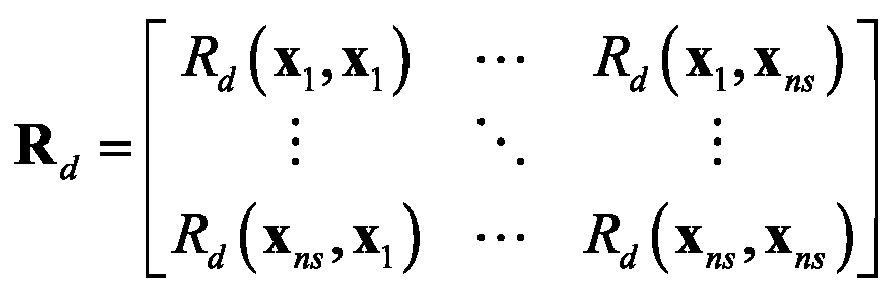


- 42) Determine an unknown parameter in the mapping relationship by using the maximum likelihood estimation method, to obtain the trained mapping relationship.
- 43) Improve the trained mapping relationship by using the EI criterion, to obtain the trained mapping relationship.
- Specifically, to improve prediction precision of the model, the EI criterion is used to find a new sample point with a maximum value of a mathematical expectation and a new sample point with an optimal objective function value in a process of training the Kriging model, and the two new sample points are used for training optimization of the model, till a convergence condition is satisfied. Ĉl(x) is used as an example, and Ĉd(x) and Ĉm(x) are similar to Ĉl(x). In the EI criterion, it is assumed that Ĉl(x) of any prediction point x is characterized by normal random distribution, in other words, satisfies Ĉl(x)--N(µ,s 2), where µ represents an average predicted value, and s represents a standard deviation. In calculation space, a mathematical expectation of any point can be calculated according to the following formula:


- Step S5: Determine an optimal sample point based on the trained mapping relationship by using NSGA-II. The optimal sample point corresponds to an optimal flow field characteristic, and the optimal flow field characteristic includes an optimal lift coefficient, an optimal drag coefficient, and an optimal moment coefficient.
- The step S5 specifically includes the following substeps:
- 501) Randomly generate an initial population whose scale is N.
- 502) Calculate, by using the trained mapping relationship, a lift coefficient, a drag coefficient, and a moment coefficient that correspond to each individual in a current-generation population.
- 503) Perform fast non-dominated sorting on all individuals in the current-generation population based on the lift coefficient, the drag coefficient, and the moment coefficient that correspond to each individual in the current-generation population, and obtain a current-generation parent population by performing selection, crossover, and mutation based on a genetic algorithm, where a quantity of population generations is equal to a quantity of iterations of the genetic algorithm.
- 504) Calculate, by using the trained mapping relationship, a lift coefficient, a drag coefficient, and a moment coefficient that correspond to each individual in the current-generation parent population.
- 505) Perform fast non-dominated sorting on all individuals in the current-generation parent population based on the lift coefficient, the drag coefficient, and the moment coefficient that correspond to each individual in the current-generation parent population, and obtain a current-generation child population by performing selection, crossover, and mutation based on the genetic algorithm.
- 506) Combine the current-generation parent population and the current-generation child population to obtain a combined current-generation population.
- 507) Calculate, by using the trained mapping relationship, a lift coefficient, a drag coefficient, and a moment coefficient that correspond to each individual in the combined current-generation population.
- 508) Perform fast non-dominated sorting on all individuals in the combined current-generation population based on the lift coefficient, the drag coefficient, and the moment coefficient that correspond to each individual in the combined current-generation population, and calculate an individual crowdedness degree in each non-dominated layer.
- 509) Select, from the combined current-generation population based on a result of fast non-dominated sorting and the individual crowdedness degree, an individual that satisfies a preset condition, to constitute a next-generation parent population.
- 510) Determine whether a sequence number of a generation to which the next-generation parent population belongs is equal to a preset maximum quantity of iterations. If the sequence number of the generation to which the next-generation parent population belongs is not equal to the preset maximum quantity of iterations, the next-generation parent population is used as a current-generation parent population, and the step 504) is performed to calculate, by using the trained mapping relationship, a lift coefficient, a drag coefficient, and a moment coefficient that correspond to each individual in the current-generation parent population. If the sequence number of the generation to which the next-generation parent population belongs is equal to the preset maximum quantity of iterations, an individual in the next-generation parent population is determined as the optimal sample point.
- Refer to
FIG. 3 . Based on the foregoing ideas, a specific process of finding an optimal airfoil by using NSGA-II is as follows: (1) Randomly generate an initial population x 1,x 2,...,x N whose scale is N. (2) Calculate Cl,Cd,Cm of each individual in the population by using the mapping relationship established based on the Kriging model. (3) Perform non-dominated sorting on an individual in the population based on values of Cl,Cd,Cm, and obtain the first-generationparent population 
child population 

child population 
- Step S6: Determining a rotor airfoil based on the optimal sample point.
- In actual application, the optimized airfoil finally obtained by performing the steps S1 to S6 is characterized by a large leading edge radius on an upper airfoil surface, a flat transition part from 0.2c to 0.4c on the upper surface, a concave lower surface, and a slightly upturned trailing edge. The optimized airfoil is manufactured based on data provided in Table 1 A chord length of the airfoil is 1.
Table 1 Data of the optimized airfoil Sequence number of a coordinate point on the lower airfoil surface Horizontal coordinate (x/c) on the lower airfoil surface Vertical coordinate (y/c) on the lower airfoil surface Sequence number of a coordinate point on the upper airfoil surface Horizontal coordinate (x/c) on the upper airfoil surface Vertical coordinate (y/c) on the upper airfoil surface 1 1.00000 0.00000 1 1.00000 0.00000 2 0.99017 -0.00179 2 0.99008 0.00047 3 0.97206 -0.00458 3 0.97142 0.00007 4 0.94635 -0.00766 4 0.94499 0.00320 5 0.91376 -0.01057 5 0.91183 0.00961 6 0.87506 -0.01315 6 0.87275 0.01872 7 0.83104 -0.01537 7 0.82834 0.02946 8 0.78244 -0.01709 8 0.77916 0.04073 9 0.73002 -0.01807 9 0.72585 0.05173 10 0.67457 -0.01811 10 0.66915 0.06189 11 0.61685 -0.01723 11 0.60982 0.07079 12 0.55762 -0.01584 12 0.54867 0.07794 13 0.49762 -0.01455 13 0.48649 0.08296 14 0.43761 -0.01395 14 0.42418 0.08588 15 0.37835 -0.01434 15 0.36260 0.08733 16 0.32061 -0.01561 16 0.30259 0.08818 17 0.26515 -0.01736 17 0.24493 0.08891 18 0.21272 -0.01914 18 0.19043 0.08895 19 0.16407 -0.02060 19 0.13994 0.08651 20 0.11994 -0.02148 20 0.09471 0.07929 21 0.08109 -0.02144 21 0.05669 0.06610 22 0.04834 -0.01991 22 0.02789 0.04813 23 0.02268 -0.01599 23 0.00957 0.02849 24 0.00577 -0.00900 24 0.00154 0.01129 25 0.00011 -0.00100 25 0.00005 0.00099 26 0.00000 0.00000 26 0.00000 0.00000 - A coordinate system and a profile of the airfoil are shown in
FIG. 4. FIG. 5 compares an SC1095 airfoil and the optimized airfoil. It can be learned fromFIG. 5 that the optimized airfoil has a larger camber, the leading edging radius on the upper airfoil surface of the optimized airfoil is obviously larger than that of the SC1095 airfoil, the flat transition part is available in the middle of the upper surface of the optimized airfoil, and the optimized airfoil is characterized by the concave lower surface and the slightly upturned trailing edge.FIG. 6 to FIG.8 compare aerodynamic characteristics of the two airfoils in a coupled condition with a changing incoming flow and a changing angle of attack. It can be learned fromFIG. 6 to FIG.8 that, compared with the SC1095 airfoil, the optimized airfoil has been greatly improved in drag and moment characteristics, thereby alleviating drag divergence and moment divergence. In addition, an area of a lift coefficient hysteresis loop of the optimized airfoil is remarkably reduced, and this indicates that the optimized airfoil can effectively improve dynamic aerodynamic characteristics of the airfoil in a rotor environment and suppress dynamic stall.FIG. 9 to FIG. 10 compare flow field characteristics of the two airfoils under three angles of attack in the coupled condition with the changing incoming flow and the changing angle of attack. It can be learned fromFIG. 9 to FIG. 10 that, when the angle of attack (α) is 17.56° in a pitching-up process, for both the SC1095 airfoil and the optimized airfoil, a vortex is generated only near a trailing edge, and a streamline attaches an airfoil surface at a leading edge and in the middle. As the angle of attack increases to 18.00°, a vortex is generated at the leading edge of the SC1095 airfoil. In addition, as the airfoil pitches down, the leading edge vortex is enhanced and gradually moves to the trailing edge until it sheds from the airfoil surface. For the optimized airfoil, an adverse pressure gradient of the leading edge is alleviated by changing the profile of the optimized airfoil, thereby suppressing the leading edge vortex. Therefore, the optimized airfoil has better dynamic characteristics. - Compared with the SC1095 airfoil, the optimized airfoil has a better dynamic stall characteristic. Reasons are as follows: (1) The optimized airfoil has a larger leading edge radius on the upper airfoil surface, and this can effectively alleviate the adverse pressure gradient of the leading edge of the airfoil (the optimized airfoil has a smaller peak negative pressure value at the leading edge, as shown in
FIG. 10 (a) and FIG. 10 (b) ), and weaken strength of the leading edge vortex and even suppress the leading edge vortex (streamline, as shown inFIG. 9 ), thereby alleviating and even avoiding a sharp drop in lift and divergence of drag and moments when the leading edge vortex moves or falls off. (2) The flat transition part from a position 0.2c to a position 0.4c is available on the upper surface of the optimized airfoil, and this can postpone drag divergence and moment divergence. (3) Positions 0.1c to 0.7c on the lower surface of the optimized airfoil are concave, increasing the camber of the airfoil and improving the lift of the airfoil. (4) The trailing edge of the optimized airfoil is slightly upturned, and this can postpone drag divergence and moment divergence, and can improve a reattaching characteristic of an airflow in the case of a large angle of attack. - According to the method for determining a helicopter rotor airfoil in this embodiment, in the condition with the changing incoming flow and the changing angle of attack, the leading edge vortex is suppressed in the entire motion process, and the vortex is generated only near the trailing edge in the case of the large angle of attack. In this way, the lift, the drag, and the moment of the airfoil are no longer affected by moving or shedding of the leading edge vortex in the dynamic stall process.
- The present disclosure further provides a system for determining a helicopter rotor airfoil.
FIG. 11 is a schematic structural diagram of a system for determining a helicopter rotor airfoil according to an embodiment of the present disclosure. Refer toFIG. 11 . The system for determining a helicopter rotor airfoil in this embodiment includes a sample point generation module 1101, an airfoil surface equation determining module 1102, a flow field characteristic calculation module 1103, a mapping relationship calculation module 1104, a multi-objective optimization module 1105, and an airfoil determining module 1106. - The sample point generation module 1101 is configured to randomly generate a sample point by using an LHS method.
- The airfoil surface equation determining module 1102 is configured to determine characterization equations of upper and lower airfoil surfaces of an airfoil based on the sample point by using a CST method.
- The flow field characteristic calculation module 1103 is configured to perform dynamic characteristic simulation on the airfoil according to the characterization equations of the upper and lower airfoil surfaces by using a CFD method, to obtain a flow field characteristic of the airfoil, where the flow field characteristic includes a lift coefficient, a drag coefficient, and a moment coefficient.
- The mapping relationship calculation module 1104 is configured to establish a mapping relationship between the sample point and the flow field characteristic by using a Kriging model, and train the mapping relationship by using a maximum likelihood estimation method and an EI criterion, to obtain a trained mapping relationship.
- The multi-objective optimization module 1105 is configured to determine an optimal sample point based on the trained mapping relationship by using NSGA-II, where the optimal sample point corresponds to an optimal flow field characteristic, and the optimal flow field characteristic includes an optimal lift coefficient, an optimal drag coefficient, and an optimal moment coefficient.
- The airfoil determining module 1106 is configured to determine a rotor airfoil based on the optimal sample point.
- Each embodiment in this specification is described in a progressive manner, each embodiment focuses on the difference from other embodiments, and the same and similar parts between the embodiments may refer to each other. For the system disclosed in the embodiments, since the system corresponds to the method disclosed in the embodiments, the system is simply described, and reference can be made to the method description.
- In this specification, several specific embodiments are used for illustration of the principles and implementations of the present disclosure. The description of the foregoing embodiments is used to help illustrate the method of the present disclosure and the core ideas thereof. In addition, those of ordinary skill in the art can make various modifications in terms of specific implementations and scope of application in accordance with the ideas of the present disclosure. In conclusion, the content of this specification shall not be construed as a limitation on the present disclosure.
Claims (10)
- A method for determining a helicopter rotor airfoil, comprising:randomly generating a sample point by using a Latin hypercube sampling (LHS) method;determining characterization equations of upper and lower airfoil surfaces of an airfoil based on the sample point by using a class shape transformation (CST) method;performing dynamic characteristic simulation on the airfoil according to the characterization equations of the upper and lower airfoil surfaces by using a computational fluid dynamics (CFD) method, to obtain a flow field characteristic of the airfoil, wherein the flow field characteristic comprises a lift coefficient, a drag coefficient, and a moment coefficient;establishing a mapping relationship between the sample point and the flow field characteristic by using a Kriging model, and training the mapping relationship by using a maximum likelihood estimation method and an expected improvement (EI) criterion, to obtain a trained mapping relationship;determining an optimal sample point based on the trained mapping relationship by using Non-dominated Sorting Genetic Algorithm II (NSGA-II), wherein the optimal sample point corresponds to an optimal flow field characteristic, and the optimal flow field characteristic comprises an optimal lift coefficient, an optimal drag coefficient, and an optimal moment coefficient; anddetermining a rotor airfoil based on the optimal sample point.
- The method for determining a helicopter rotor airfoil according to claim 1, wherein the characterization equations of the upper and lower airfoil surfaces are as follows:

TE / c, Δzl = ylTE / c ; Δzu represents a dimensionless trailing edge thickness of the upper airfoil surface of the airfoil; Δzl represents a dimensionless trailing edge thickness of the lower airfoil surface of the airfoil; yuTE represents a vertical coordinate of a trailing edge point on the upper airfoil surface of the airfoil; YlTE represents a vertical coordinate of a trailing edge point on the lower airfoil surface of the airfoil; C(ζ)=ζ N1·(1-ζ) N2; C(ζ) represents a class function; N 1 and N 2 are both constants;


- The method for determining a helicopter rotor airfoil according to claim 1, wherein the performing dynamic characteristic simulation on the airfoil according to the characterization equations of the upper and lower airfoil surfaces by using a CFD method, to obtain a flow field characteristic of the airfoil specifically comprises:determining coordinates of the sample point according to the characterization equations of the upper and lower airfoil surfaces;determining an initial grid, wherein the initial grid is generated based on the coordinates of the sample point;generating, based on the initial grid and by using a Poisson equation-based elliptic equation grid generation method, a C-shaped body-fitted grid around the airfoil, wherein the Poisson equation is as follows:
 wherein (ξ,η) represents a point in a curvilinear coordinate system under a calculation plane, there is a mapping relationship between (ξ,η) and a point (ζ,Ψ) in a linear coordinate system under a physical plane,


 calculating an area and a volume of each grid cell in the C-shaped body-fitted grid;determining a fluid control equation based on the area, the volume, a conservative variable, a convective flux term, and a viscous flux term, wherein the fluid control equation is as follows:
 wherein t represents physical time, Fc represents the convective flux term, Fv represents the viscous flux term, Ω represents the volume of the grid cell, S represents the area of the grid cell, W represents the conservative variable,
 ρ represents air density, E represents total energy, H represents total enthalpy, p represents intensity of pressure, u represents a velocity component in an x-axis direction, v represents a velocity component in a y-axis direction, Vr represents a velocity of relative motion, Vt represents a grid moving velocity, (nx,ny ) represents a unit normal vector of a grid cell surface, τxx represents a viscous stress component acting on a plane perpendicular to an x axis and along the x-axis direction, τxy represents a viscous stress component acting on the plane perpendicular to the x axis and along the y-axis direction, τyy represents a viscous stress component acting on a plane perpendicular to a y axis and along the y-axis direction, Θ x represents a viscous stress term, and Θ y represents a heat conduction term;solving the fluid control equation, wherein a solution of the fluid control equation is
 calculating the flow field characteristic of the airfoil based on the solution of the fluid control equation.
 - The method for determining a helicopter rotor airfoil according to claim 1, wherein the establishing a mapping relationship between the sample point and the flow field characteristic by using a Kriging model, and training the mapping relationship by using a maximum likelihood estimation method and an EI criterion, to obtain a trained mapping relationship specifically comprises:establishing the mapping relationship between the sample point and the flow field characteristic by using the Kriging model, wherein the mapping relationship is as follows:


 wherein Ĉl represents a predicted value of the lift coefficient, Ĉd represents a predicted value of the drag coefficient, Ĉm represents a predicted value of the moment coefficient, Y l represents a vector constituted by lift coefficients Cl corresponding to sample points, Y d represents a vector constituted by drag coefficients Cd corresponding to the sample points, Y m represents a vector constituted by moment coefficients Cm corresponding to the sample points, Y l =[Cl 1 Cl 2 ... Clns ] T , Yd =[Cd 1 Cd 2 ... Cdns ] T, Y m =[Cm 1 Cm 2 ... Cmns ] T , ns represents a quantity of the sample points,





 determining an unknown parameter in the mapping relationship by using the maximum likelihood estimation method, to obtain the trained mapping relationship; andimproving the trained mapping relationship by using the EI criterion, to obtain the trained mapping relationship.
 - The method for determining a helicopter rotor airfoil according to claim 1, wherein the determining an optimal sample point based on the trained mapping relationship by using NSGA-II specifically comprises:randomly generating an initial population whose scale is N;calculating, by using the trained mapping relationship, a lift coefficient, a drag coefficient, and a moment coefficient that correspond to each individual in a current-generation population;performing fast non-dominated sorting on all individuals in the current-generation population based on the lift coefficient, the drag coefficient, and the moment coefficient that correspond to each individual in the current-generation population, and obtaining a current-generation parent population by performing selection, crossover, and mutation based on a genetic algorithm, wherein a quantity of population generations is equal to a quantity of iterations of the genetic algorithm;calculating, by using the trained mapping relationship, a lift coefficient, a drag coefficient, and a moment coefficient that correspond to each individual in the current-generation parent population;performing fast non-dominated sorting on all individuals in the current-generation parent population based on the lift coefficient, the drag coefficient, and the moment coefficient that correspond to each individual in the current-generation parent population, and obtaining a current-generation child population by performing selection, crossover, and mutation based on the genetic algorithm;combining the current-generation parent population and the current-generation child population to obtain a combined current-generation population;calculating, by using the trained mapping relationship, a lift coefficient, a drag coefficient, and a moment coefficient that correspond to each individual in the combined current-generation population;performing fast non-dominated sorting on all individuals in the combined current-generation population based on the lift coefficient, the drag coefficient, and the moment coefficient that correspond to each individual in the combined current-generation population, and calculating an individual crowdedness degree in each non-dominated layer;selecting, from the combined current-generation population based on a result of fast non-dominated sorting and the individual crowdedness degree, an individual that satisfies a preset condition, to constitute a next-generation parent population;determining whether a sequence number of a generation to which the next-generation parent population belongs is equal to a preset maximum quantity of iterations; andif the sequence number of the generation to which the next-generation parent population belongs is not equal to the preset maximum quantity of iterations, using the next-generation parent population as a current-generation parent population, and returning to the step of calculating, by using the trained mapping relationship, a lift coefficient, a drag coefficient, and a moment coefficient that correspond to each individual in the current-generation parent population; orif the sequence number of the generation to which the next-generation parent population belongs is equal to the preset maximum quantity of iterations, determining an individual in the next-generation parent population as the optimal sample point.
- A system for determining a helicopter rotor airfoil, comprising:a sample point generation module, configured to randomly generate a sample point by using an LHS method;an airfoil surface equation determining module, configured to determine characterization equations of upper and lower airfoil surfaces of an airfoil based on the sample point by using a CST method;a flow field characteristic calculation module, configured to perform dynamic characteristic simulation on the airfoil according to the characterization equations of the upper and lower airfoil surfaces by using a CFD method, to obtain a flow field characteristic of the airfoil, wherein the flow field characteristic comprises a lift coefficient, a drag coefficient, and a moment coefficient;a mapping relationship calculation module, configured to establish a mapping relationship between the sample point and the flow field characteristic by using a Kriging model, and train the mapping relationship by using a maximum likelihood estimation method and an EI criterion, to obtain a trained mapping relationship;a multi-objective optimization module, configured to determine an optimal sample point based on the trained mapping relationship by using NSGA-II, wherein the optimal sample point corresponds to an optimal flow field characteristic, and the optimal flow field characteristic comprises an optimal lift coefficient, an optimal drag coefficient, and an optimal moment coefficient; andan airfoil determining module, configured to determine a rotor airfoil based on the optimal sample point.
- The system for determining a helicopter rotor airfoil according to claim 6, wherein the characterization equations of the upper and lower airfoil surfaces are as follows:

TE /c, Δzl = ylTE /c; Δzu represents a dimensionless trailing edge thickness of the upper airfoil surface of the airfoil; Δzl represents a dimensionless trailing edge thickness of the lower airfoil surface of the airfoil; yuTE represents a vertical coordinate of a trailing edge point on the upper airfoil surface of the airfoil; YlTE represents a vertical coordinate of a trailing edge point on the lower airfoil surface of the airfoil; C(ζ)=ζ N1·(1-ζ) N2; C(ζ) represents a class function; N 1 and N 2 are both constants;


- The system for determining a helicopter rotor airfoil according to claim 6, wherein the flow field characteristic calculation module specifically comprises:a coordinate determining unit, configured to determine coordinates of the sample point according to the characterization equations of the upper and lower airfoil surfaces;an initial grid determining unit, configured to determine an initial grid, wherein the initial grid is generated based on the coordinates of the sample point;a body-fitted grid generation unit, configured to generate, based on the initial grid and by using a Poisson equation-based elliptic equation grid generation method, a C-shaped body-fitted grid around the airfoil, wherein the Poisson equation is as follows:
 wherein (ξ,η) represents a point in a curvilinear coordinate system under a calculation plane, there is a mapping relationship between (ξ,η) and a point (ζ,Ψ) in a linear coordinate system under a physical plane,


 a grid parameter calculation unit, configured to calculate an area and a volume of each grid cell in the C-shaped body-fitted grid;a fluid control equation determining unit, configured to determine a fluid control equation based on the area, the volume, a conservative variable, a convective flux term, and a viscous flux term, wherein the fluid control equation is as follows:
 wherein t represents physical time, Fc represents the convective flux term, Fv represents the viscous flux term, Ω represents the volume of the grid cell, S represents the area of the grid cell, W represents the conservative variable,
 ρ represents air density, E represents total energy, H represents total enthalpy, p represents intensity of pressure, u represents a velocity component in an x-axis direction, v represents a velocity component in a y-axis direction, Vr represents a velocity of relative motion, Vt represents a grid moving velocity, (nx ,ny ) represents a unit normal vector of a grid cell surface, τxx represents a viscous stress component acting on a plane perpendicular to an x axis and along the x-axis direction, τxy represents a viscous stress component acting on the plane perpendicular to the x axis and along the y-axis direction, τyy represents a viscous stress component acting on a plane perpendicular to a y axis and along the y-axis direction, Θ x represents a viscous stress term, and Θ y represents a heat conduction term;a solving unit, configured to solve the fluid control equation, wherein a solution of the fluid control equation is
 a flow field characteristic determining unit, configured to calculate the flow field characteristic of the airfoil based on the solution of the fluid control equation.
 - The system for determining a helicopter rotor airfoil according to claim 6, wherein the mapping relationship calculation module specifically comprises:a mapping relationship determining unit, configured to establish the mapping relationship between the sample point and the flow field characteristic by using the Kriging model, wherein the mapping relationship is as follows:


 wherein Ĉl represents a predicted value of the lift coefficient, Ĉd represents a predicted value of the drag coefficient, Ĉm represents a predicted value of the moment coefficient, Y l represents a vector constituted by lift coefficients Cl corresponding to sample points, Y d represents a vector constituted by drag coefficients Cd corresponding to the sample points, Y m represents a vector constituted by moment coefficients Cm corresponding to the sample points, Y l = [Cl 1 Cl 2 ... Clns ] T , Yd = [Cd 1 Cd 2 ... Cdns ] T, Y m =[Cm 1 Cm 2 ... Cm ns] T , ns represents a quantity of the sample points,
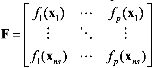


 a first training unit, configured to determine an unknown parameter in the mapping relationship by using the maximum likelihood estimation method, to obtain the trained mapping relationship; anda second training unit, configured to improve the trained mapping relationship by using the EI criterion, to obtain the trained mapping relationship.
 - The system for determining a helicopter rotor airfoil according to claim 6, wherein the multi-objective optimization module specifically comprises:an initial-population generation unit, configured to randomly generate an initial population whose scale is N;a first calculation unit, configured to calculate, by using the trained mapping relationship, a lift coefficient, a drag coefficient, and a moment coefficient that correspond to each individual in a current-generation population;a first sorting unit, configured to perform fast non-dominated sorting on all individuals in the current-generation population based on the lift coefficient, the drag coefficient, and the moment coefficient that correspond to each individual in the current-generation population, and obtain a current-generation parent population by performing selection, crossover, and mutation based on a genetic algorithm, wherein a quantity of population generations is equal to a quantity of iterations of the genetic algorithm;a second calculation unit, configured to calculate, by using the trained mapping relationship, a lift coefficient, a drag coefficient, and a moment coefficient that correspond to each individual in the current-generation parent population;a second sorting unit, configured to perform fast non-dominated sorting on all individuals in the current-generation parent population based on the lift coefficient, the drag coefficient, and the moment coefficient that correspond to each individual in the current-generation parent population, and obtain a current-generation child population by performing selection, crossover, and mutation based on the genetic algorithm;a population combination unit, configured to combine the current-generation parent population and the current-generation child population to obtain a combined current-generation population;a third calculation unit, configured to calculate, by using the trained mapping relationship, a lift coefficient, a drag coefficient, and a moment coefficient that correspond to each individual in the combined current-generation population;a second sorting unit, configured to perform fast non-dominated sorting on all individuals in the combined current-generation population based on the lift coefficient, the drag coefficient, and the moment coefficient that correspond to each individual in the combined current-generation population, and calculate an individual crowdedness degree in each non-dominated layer;an individual selection unit, configured to select, from the combined current-generation population based on a result of fast non-dominated sorting and the individual crowdedness degree, an individual that satisfies a preset condition, to constitute a next-generation parent population; anda determining unit, configured to determine whether a sequence number of a generation to which the next-generation parent population belongs is equal to a preset maximum quantity of iterations; if the sequence number of the generation to which the next-generation parent population belongs is not equal to the preset maximum quantity of iterations, use the next-generation parent population as a current-generation parent population, and perform the operation performed by the second calculation unit; or if the sequence number of the generation to which the next-generation parent population belongs is equal to the preset maximum quantity of iterations, determine an individual in the next-generation parent population as the optimal sample point.
Applications Claiming Priority (2)
| Application Number | Priority Date | Filing Date | Title |
|---|---|---|---|
| CN201911017404.0A CN110705126A (en) | 2019-10-24 | 2019-10-24 | A method and system for determining the airfoil of a helicopter rotor |
| PCT/CN2020/107732 WO2021077855A1 (en) | 2019-10-24 | 2020-08-07 | Helicopter rotor airfoil determination method and system |
Publications (2)
| Publication Number | Publication Date |
|---|---|
| EP3926507A1 true EP3926507A1 (en) | 2021-12-22 |
| EP3926507A4 EP3926507A4 (en) | 2022-05-18 |
Family
ID=69202130
Family Applications (1)
| Application Number | Title | Priority Date | Filing Date |
|---|---|---|---|
| EP20879600.3A Withdrawn EP3926507A4 (en) | 2019-10-24 | 2020-08-07 | METHOD AND SYSTEM FOR HELICOPTER ROTOR AERODYNAMIC PROFILE DETERMINATION |
Country Status (5)
| Country | Link |
|---|---|
| US (1) | US11423201B2 (en) |
| EP (1) | EP3926507A4 (en) |
| JP (1) | JP7092421B2 (en) |
| CN (1) | CN110705126A (en) |
| WO (1) | WO2021077855A1 (en) |
Cited By (1)
| Publication number | Priority date | Publication date | Assignee | Title |
|---|---|---|---|---|
| CN119808280A (en) * | 2025-03-07 | 2025-04-11 | 西北工业大学 | Design method and family of thin airfoils with wide speed range and wide frequency band for wing-body fusion layout |
Families Citing this family (48)
| Publication number | Priority date | Publication date | Assignee | Title |
|---|---|---|---|---|
| CN110705126A (en) * | 2019-10-24 | 2020-01-17 | 南京航空航天大学 | A method and system for determining the airfoil of a helicopter rotor |
| CN111310282A (en) * | 2020-03-26 | 2020-06-19 | 南京航空航天大学 | Helicopter rotor wing profile generation method and system suitable for plateau environment |
| CN111553086B (en) * | 2020-04-30 | 2023-01-03 | 南京航空航天大学 | Helicopter duct tail rotor inner wall surface shape determining method and system |
| CN111625901B (en) * | 2020-05-07 | 2022-05-31 | 中国空气动力研究与发展中心计算空气动力研究所 | Intelligent pressure coefficient curve generation method for wing profile |
| CN111814246B (en) * | 2020-06-11 | 2022-09-27 | 中国空气动力研究与发展中心计算空气动力研究所 | Wing section inverse design method based on generation countermeasure network |
| CN112199784B (en) * | 2020-11-04 | 2022-05-31 | 南京航空航天大学 | Coaxial rigid double-rotor pneumatic balancing method and system |
| CN112991137B (en) * | 2021-04-26 | 2021-08-20 | 湖南映客互娱网络信息有限公司 | Method for dynamically identifying and removing watermark position of picture |
| CN114386177B (en) * | 2022-01-18 | 2024-11-15 | 西北工业大学 | A grey estimation method for drag coefficient of flying wing glider airfoil |
| CN114722498A (en) * | 2022-04-02 | 2022-07-08 | 浙江大学 | Wing section design method based on generation of countermeasure network |
| CN114987755B (en) * | 2022-05-18 | 2023-04-25 | 南京航空航天大学 | Automatic wing profile modification method for parafoil |
| CN115169258B (en) * | 2022-07-01 | 2025-05-30 | 南京航空航天大学 | A method and system for extracting lift and drag coefficient of rotor profile |
| CN115358001B (en) * | 2022-07-22 | 2025-09-23 | 中国空气动力研究与发展中心空天技术研究所 | A method for comprehensive optimization of aerodynamic stealth and leading edge radius of a flying wing aircraft |
| CN115795642B (en) * | 2022-09-08 | 2025-11-11 | 西北工业大学 | Airfoil type optimal design method and system special for high-speed train |
| CN115270362B (en) * | 2022-09-30 | 2023-01-24 | 北京科技大学 | Method and device for blade configuration design optimization under rated working conditions of centrifugal compressor |
| CN115481510B (en) * | 2022-09-30 | 2023-05-02 | 北京科技大学 | Radial compressor blade multi-working-condition optimization method and device based on improved NSGA-II algorithm |
| CN115659504B (en) * | 2022-10-26 | 2025-08-29 | 南京航空航天大学 | A multidisciplinary integrated high-altitude paraglider automatic optimization design method |
| CN115659823B (en) * | 2022-11-02 | 2026-04-14 | 中国航空工业集团公司沈阳空气动力研究所 | Airfoil aerodynamic coefficient prediction method based on attribute reduction, electronic equipment and storage medium |
| CN115423053B (en) * | 2022-11-07 | 2023-04-07 | 中国空气动力研究与发展中心计算空气动力研究所 | Method and related equipment for classifying unstructured flow field data suitable for airfoil section |
| CN115618498B (en) * | 2022-11-08 | 2023-03-10 | 中国空气动力研究与发展中心计算空气动力研究所 | Prediction method, device, equipment and medium for cross-basin flow field of aircraft |
| CN116205154B (en) * | 2022-12-30 | 2023-09-05 | 中国能源建设集团广东省电力设计研究院有限公司 | Aerodynamic coefficient generation method and device, terminal equipment and storage medium |
| CN118410607A (en) * | 2023-02-23 | 2024-07-30 | 成都航空职业技术学院 | A method for local smoothing of airfoil |
| CN118410606A (en) * | 2023-02-23 | 2024-07-30 | 成都航空职业技术学院 | A global smoothing method for airfoil |
| CN116796915B (en) * | 2023-04-18 | 2024-01-12 | 中南大学 | Proxy model method for intelligent railway route selection |
| CN116304578B (en) * | 2023-04-20 | 2026-02-06 | 北京航空航天大学 | Wing dynamic stall flow state prediction method and system |
| CN116882311B (en) * | 2023-06-13 | 2024-04-23 | 兰州交通大学 | Computational fluid dynamics determination method for normalized working attack angle of lift wing of high-speed train |
| CN116767487B (en) * | 2023-06-21 | 2025-06-24 | 西北工业大学 | Blunt trailing edge weak separation low-resistance airfoil designed based on front-back symmetrical appearance of uniform incoming flow condition |
| CN116767486B (en) * | 2023-06-21 | 2025-06-24 | 西北工业大学 | Laminar flow supercritical rotor wing profile suitable for unbalanced high-speed characteristic in middle of high-speed helicopter blade |
| CN116628894B (en) * | 2023-07-20 | 2023-09-29 | 中国海洋大学 | Hydrofoil design optimization method and hydrofoil design optimization framework based on deep learning |
| CN117022588B (en) * | 2023-08-08 | 2024-03-26 | 中山大学 | Hydrofoil structure optimization method, system, equipment and medium based on Kriging model |
| CN117113571B (en) * | 2023-08-24 | 2024-07-30 | 江苏大学 | A CST parameterization method for airfoil after rotation and translation transformation |
| CN117313237B (en) * | 2023-09-23 | 2024-04-16 | 哈尔滨工业大学 | Special unmanned aerial vehicle configuration scheme optimization method based on machine learning |
| CN117485579A (en) * | 2023-10-17 | 2024-02-02 | 北京中航智科技有限公司 | A quick matching method for UAV rocket-assisted launch parameters |
| CN117508694A (en) * | 2023-10-25 | 2024-02-06 | 青州耐威智能科技有限公司 | A new airfoil for low-speed and long-endurance drones |
| CN117634334B (en) * | 2023-10-27 | 2024-07-23 | 西北工业大学 | Fighter aircraft wing profile optimization design method considering pneumatic/stealth and wide-speed-domain wing profile family |
| CN117740307B (en) * | 2024-02-18 | 2024-05-14 | 中国空气动力研究与发展中心低速空气动力研究所 | Method for predicting performance of full-size rotor wing |
| CN118332684B (en) * | 2024-03-26 | 2025-05-13 | 四川大学 | Flow field prediction method based on dense convolution network |
| CN118332898B (en) * | 2024-03-26 | 2024-11-26 | 四川大学 | Airfoil Flow Field Prediction Method Based on Hybrid Neural Network |
| CN118350292B (en) * | 2024-06-18 | 2024-08-16 | 中国空气动力研究与发展中心低速空气动力研究所 | Airfoil flow field prediction network training method, network, prediction method and medium |
| CN118378569B (en) * | 2024-06-24 | 2024-08-23 | 中国空气动力研究与发展中心计算空气动力研究所 | Modeling and calculating method for transition flow field average speed profile |
| CN118485007B (en) * | 2024-07-15 | 2024-09-27 | 北京易动宇航科技有限公司 | Multi-working-task electric propeller optimization method and system |
| CN118821325B (en) * | 2024-07-31 | 2025-11-28 | 西北工业大学 | Optimized design method for many targets of conduit propeller |
| CN118917003B (en) * | 2024-10-11 | 2025-03-18 | 西北工业大学 | Unsteady aerodynamic modeling method for compound control configuration for high angle of attack maneuvers |
| CN119312491B (en) * | 2024-11-21 | 2025-09-26 | 北京航空航天大学 | A wing aerodynamic shape optimization method for the conceptual design stage |
| CN119558009B (en) * | 2025-01-24 | 2025-04-22 | 河北工业大学 | Rudder wing structure optimization method and system for high overload environment |
| CN120145542B (en) * | 2025-02-14 | 2025-11-11 | 西北工业大学 | Airfoil parameterization method based on autoencoder model |
| CN120509114B (en) * | 2025-05-14 | 2025-11-25 | 中国航空研究院 | Airfoil Bayesian optimization method and apparatus with pressure distribution-guided target constraints |
| CN120197298B (en) * | 2025-05-21 | 2025-08-15 | 北京航空航天大学 | Airfoil robustness optimization design method considering deformation influence of flexible skin |
| CN121683630B (en) * | 2026-02-11 | 2026-04-17 | 中国空气动力研究与发展中心计算空气动力研究所 | A CFD simulation method for rotor disk chamfering |
Family Cites Families (11)
| Publication number | Priority date | Publication date | Assignee | Title |
|---|---|---|---|---|
| US4519746A (en) * | 1981-07-24 | 1985-05-28 | United Technologies Corporation | Airfoil blade |
| JP4557397B2 (en) * | 2000-09-05 | 2010-10-06 | 本田技研工業株式会社 | Blade shape design method and information medium |
| CN102298329B (en) * | 2011-08-19 | 2013-05-08 | 北京航空航天大学 | Small-size unmanned rotary wing aircraft dynamic model identification method based on adaptive genetic algorithm |
| EP3112258B1 (en) * | 2015-07-03 | 2017-09-13 | AIRBUS HELICOPTERS DEUTSCHLAND GmbH | Airfoils for rotor blades of rotary wing aircrafts |
| US20170046968A1 (en) * | 2015-08-11 | 2017-02-16 | The Boeing Company | Flight simulation modeling of aircraft dynamic stall aerodynamics |
| CN106021808A (en) * | 2016-06-07 | 2016-10-12 | 西北工业大学 | Low span chord ratio aerofoil type designing method considering three-dimensional effect |
| CN106741924A (en) * | 2016-11-20 | 2017-05-31 | 西北工业大学 | A kind of high lift-drag ratio Low-torque characteristic 9% thickness rotor-blade airfoil under the conditions of full working scope |
| US11459093B2 (en) * | 2018-02-22 | 2022-10-04 | Aviation Partners, Inc. | Winglet airfoils |
| EP3543108A1 (en) * | 2018-03-22 | 2019-09-25 | Facebook, Inc. | Automatic airfoil and wing design based on dynamic modeling of structural and aerodynamic performance |
| CN110334449A (en) * | 2019-07-04 | 2019-10-15 | 南京航空航天大学 | A kind of aerofoil profile Fast design method based on online agent model algorithm |
| CN110705126A (en) * | 2019-10-24 | 2020-01-17 | 南京航空航天大学 | A method and system for determining the airfoil of a helicopter rotor |
-
2019
- 2019-10-24 CN CN201911017404.0A patent/CN110705126A/en active Pending
-
2020
- 2020-08-07 WO PCT/CN2020/107732 patent/WO2021077855A1/en not_active Ceased
- 2020-08-07 EP EP20879600.3A patent/EP3926507A4/en not_active Withdrawn
- 2020-08-07 US US17/312,336 patent/US11423201B2/en active Active
- 2020-08-07 JP JP2021525694A patent/JP7092421B2/en active Active
Cited By (1)
| Publication number | Priority date | Publication date | Assignee | Title |
|---|---|---|---|---|
| CN119808280A (en) * | 2025-03-07 | 2025-04-11 | 西北工业大学 | Design method and family of thin airfoils with wide speed range and wide frequency band for wing-body fusion layout |
Also Published As
| Publication number | Publication date |
|---|---|
| US11423201B2 (en) | 2022-08-23 |
| JP7092421B2 (en) | 2022-06-28 |
| US20220033062A1 (en) | 2022-02-03 |
| EP3926507A4 (en) | 2022-05-18 |
| JP2022508097A (en) | 2022-01-19 |
| WO2021077855A1 (en) | 2021-04-29 |
| CN110705126A (en) | 2020-01-17 |
Similar Documents
| Publication | Publication Date | Title |
|---|---|---|
| EP3926507A1 (en) | Helicopter rotor airfoil determination method and system | |
| Medida et al. | Application of the correlation-based gamma-re theta t transition model to the spalart-allmaras turbulence model | |
| Weishuang et al. | Aerodynamic optimization and mechanism design of flexible variable camber trailing-edge flap | |
| Hu et al. | Adjoint-based aerodynamic optimization of supersonic biplane airfoils | |
| CN109484623A (en) | Wide speed domain lift line slope symmetrical airfoil design method and aerofoil profile | |
| CN106126860B (en) | A kind of hypersonic wing Robust Optimal Design for considering mismachining tolerance | |
| Berci et al. | Multidisciplinary multifidelity optimisation of a flexible wing aerofoil with reference to a small UAV | |
| CN102235325B (en) | Method for designing airfoil section of blade tip of wind machine based on airfoil section integration and mixed trailing edge modification | |
| Chen et al. | Improvement of airfoil design using smooth curvature technique | |
| CN118504144B (en) | Variable camber pneumatic optimization design method for aircraft wing with multiple trailing edge control surfaces | |
| CN110516318B (en) | Airfoil Design Method Based on Radial Basis Function Neural Network Proxy Model | |
| CN112373673B (en) | Flow control method of leading edge double bulge structure to improve double bulge airfoil performance | |
| Fatahian et al. | Numerical study of the effect of suction at a compressible and high Reynolds number flow to control the flow separation over Naca 2415 airfoil | |
| CN103488847A (en) | Aerodynamic shape optimization method based on neural network integration | |
| CN111310282A (en) | Helicopter rotor wing profile generation method and system suitable for plateau environment | |
| Molina et al. | Aerodynamics of a pitching and heaving airfoil in ground effect | |
| Eijkelhof | Design and optimisation framework of a multi-MW airborne wind energy reference system | |
| Sudhi et al. | Practical implications of conical flow assumption in nlf and hlfc wing design | |
| Zhang et al. | Multi-point optimization of transonic wing by real-coded genetic algorithm | |
| Kumar et al. | Aerodynamic Performance Optimization of Multiple Slat Airfoil based on Multi-Objective Genetic Algorithm | |
| Oda et al. | Studies on wingtip geometries by optimum spanwise lift distribution design method | |
| Molinari et al. | Aero-structural optimization of 3-D adaptive wings with embedded smart actuators | |
| Paredes et al. | Aerodynamic Design Optimization for Natural Laminar Flow Airfoils | |
| Obayashi et al. | Transonic wing design by inverse optimization using MOGA | |
| CN118504138B (en) | Design method of hypersonic natural laminar wing considering strong cross flow effect |
Legal Events
| Date | Code | Title | Description |
|---|---|---|---|
| STAA | Information on the status of an ep patent application or granted ep patent |
Free format text: STATUS: THE INTERNATIONAL PUBLICATION HAS BEEN MADE |
|
| PUAI | Public reference made under article 153(3) epc to a published international application that has entered the european phase |
Free format text: ORIGINAL CODE: 0009012 |
|
| STAA | Information on the status of an ep patent application or granted ep patent |
Free format text: STATUS: REQUEST FOR EXAMINATION WAS MADE |
|
| 17P | Request for examination filed |
Effective date: 20210916 |
|
| AK | Designated contracting states |
Kind code of ref document: A1 Designated state(s): AL AT BE BG CH CY CZ DE DK EE ES FI FR GB GR HR HU IE IS IT LI LT LU LV MC MK MT NL NO PL PT RO RS SE SI SK SM TR |
|
| A4 | Supplementary search report drawn up and despatched |
Effective date: 20220420 |
|
| RIC1 | Information provided on ipc code assigned before grant |
Ipc: B64F 5/00 20170101ALI20220412BHEP Ipc: G06F 119/14 20200101ALI20220412BHEP Ipc: B64C 27/467 20060101ALI20220412BHEP Ipc: G06N 5/00 20060101ALI20220412BHEP Ipc: G06N 3/12 20060101ALI20220412BHEP Ipc: G06F 30/28 20200101ALI20220412BHEP Ipc: G06F 30/15 20200101ALI20220412BHEP Ipc: G06F 30/20 20200101AFI20220412BHEP |
|
| DAV | Request for validation of the european patent (deleted) | ||
| DAX | Request for extension of the european patent (deleted) | ||
| STAA | Information on the status of an ep patent application or granted ep patent |
Free format text: STATUS: EXAMINATION IS IN PROGRESS |
|
| 17Q | First examination report despatched |
Effective date: 20231211 |
|
| GRAP | Despatch of communication of intention to grant a patent |
Free format text: ORIGINAL CODE: EPIDOSNIGR1 |
|
| STAA | Information on the status of an ep patent application or granted ep patent |
Free format text: STATUS: GRANT OF PATENT IS INTENDED |
|
| RIC1 | Information provided on ipc code assigned before grant |
Ipc: G06F 30/20 20200101AFI20250625BHEP Ipc: G06F 30/15 20200101ALI20250625BHEP Ipc: G06F 30/28 20200101ALI20250625BHEP Ipc: G06N 3/126 20230101ALI20250625BHEP Ipc: G06N 5/00 20060101ALI20250625BHEP Ipc: B64F 5/00 20170101ALI20250625BHEP Ipc: G06F 119/14 20200101ALI20250625BHEP Ipc: G06F 113/08 20200101ALI20250625BHEP Ipc: B64C 27/467 20060101ALI20250625BHEP Ipc: G06F 111/06 20200101ALN20250625BHEP Ipc: G06F 111/10 20200101ALN20250625BHEP |
|
| INTG | Intention to grant announced |
Effective date: 20250707 |
|
| STAA | Information on the status of an ep patent application or granted ep patent |
Free format text: STATUS: THE APPLICATION IS DEEMED TO BE WITHDRAWN |
|
| 18D | Application deemed to be withdrawn |
Effective date: 20251108 |