EP3905141A1 - Estimating the implicit likelihoods of generative adversarial networks - Google Patents
Estimating the implicit likelihoods of generative adversarial networks Download PDFInfo
- Publication number
- EP3905141A1 EP3905141A1 EP20215923.2A EP20215923A EP3905141A1 EP 3905141 A1 EP3905141 A1 EP 3905141A1 EP 20215923 A EP20215923 A EP 20215923A EP 3905141 A1 EP3905141 A1 EP 3905141A1
- Authority
- EP
- European Patent Office
- Prior art keywords
- network
- input data
- latent variable
- trained
- variance
- Prior art date
- Legal status (The legal status is an assumption and is not a legal conclusion. Google has not performed a legal analysis and makes no representation as to the accuracy of the status listed.)
- Granted
Links
Images



Classifications
-
- G—PHYSICS
- G06—COMPUTING OR CALCULATING; COUNTING
- G06F—ELECTRIC DIGITAL DATA PROCESSING
- G06F18/00—Pattern recognition
- G06F18/20—Analysing
- G06F18/21—Design or setup of recognition systems or techniques; Extraction of features in feature space; Blind source separation
- G06F18/214—Generating training patterns; Bootstrap methods, e.g. bagging or boosting
-
- G—PHYSICS
- G06—COMPUTING OR CALCULATING; COUNTING
- G06N—COMPUTING ARRANGEMENTS BASED ON SPECIFIC COMPUTATIONAL MODELS
- G06N3/00—Computing arrangements based on biological models
- G06N3/02—Neural networks
- G06N3/08—Learning methods
- G06N3/088—Non-supervised learning, e.g. competitive learning
-
- G—PHYSICS
- G06—COMPUTING OR CALCULATING; COUNTING
- G06F—ELECTRIC DIGITAL DATA PROCESSING
- G06F18/00—Pattern recognition
- G06F18/20—Analysing
- G06F18/23—Clustering techniques
- G06F18/232—Non-hierarchical techniques
- G06F18/2321—Non-hierarchical techniques using statistics or function optimisation, e.g. modelling of probability density functions
- G06F18/23213—Non-hierarchical techniques using statistics or function optimisation, e.g. modelling of probability density functions with fixed number of clusters, e.g. K-means clustering
-
- G—PHYSICS
- G06—COMPUTING OR CALCULATING; COUNTING
- G06N—COMPUTING ARRANGEMENTS BASED ON SPECIFIC COMPUTATIONAL MODELS
- G06N3/00—Computing arrangements based on biological models
- G06N3/02—Neural networks
- G06N3/04—Architecture, e.g. interconnection topology
- G06N3/045—Combinations of networks
-
- G—PHYSICS
- G06—COMPUTING OR CALCULATING; COUNTING
- G06N—COMPUTING ARRANGEMENTS BASED ON SPECIFIC COMPUTATIONAL MODELS
- G06N3/00—Computing arrangements based on biological models
- G06N3/02—Neural networks
- G06N3/04—Architecture, e.g. interconnection topology
- G06N3/0464—Convolutional networks [CNN, ConvNet]
-
- G—PHYSICS
- G06—COMPUTING OR CALCULATING; COUNTING
- G06N—COMPUTING ARRANGEMENTS BASED ON SPECIFIC COMPUTATIONAL MODELS
- G06N3/00—Computing arrangements based on biological models
- G06N3/02—Neural networks
- G06N3/04—Architecture, e.g. interconnection topology
- G06N3/047—Probabilistic or stochastic networks
-
- G—PHYSICS
- G06—COMPUTING OR CALCULATING; COUNTING
- G06N—COMPUTING ARRANGEMENTS BASED ON SPECIFIC COMPUTATIONAL MODELS
- G06N3/00—Computing arrangements based on biological models
- G06N3/02—Neural networks
- G06N3/04—Architecture, e.g. interconnection topology
- G06N3/0475—Generative networks
-
- G—PHYSICS
- G06—COMPUTING OR CALCULATING; COUNTING
- G06N—COMPUTING ARRANGEMENTS BASED ON SPECIFIC COMPUTATIONAL MODELS
- G06N3/00—Computing arrangements based on biological models
- G06N3/02—Neural networks
- G06N3/08—Learning methods
-
- G—PHYSICS
- G06—COMPUTING OR CALCULATING; COUNTING
- G06N—COMPUTING ARRANGEMENTS BASED ON SPECIFIC COMPUTATIONAL MODELS
- G06N3/00—Computing arrangements based on biological models
- G06N3/02—Neural networks
- G06N3/08—Learning methods
- G06N3/084—Backpropagation, e.g. using gradient descent
-
- G—PHYSICS
- G06—COMPUTING OR CALCULATING; COUNTING
- G06N—COMPUTING ARRANGEMENTS BASED ON SPECIFIC COMPUTATIONAL MODELS
- G06N3/00—Computing arrangements based on biological models
- G06N3/02—Neural networks
- G06N3/08—Learning methods
- G06N3/094—Adversarial learning
-
- G—PHYSICS
- G06—COMPUTING OR CALCULATING; COUNTING
- G06N—COMPUTING ARRANGEMENTS BASED ON SPECIFIC COMPUTATIONAL MODELS
- G06N5/00—Computing arrangements using knowledge-based models
- G06N5/04—Inference or reasoning models
Definitions
- the present disclosure relates generally to systems and methods for computer learning that can provide improved computer performance, features, and uses. More particularly, the present disclosure relates to embodiments for estimating the implicit likelihoods of generative adversarial networks (GANs).
- GANs generative adversarial networks
- GANs generative adversarial networks
- the generator in a GAN can be seen as a nonlinear parametric mapping from the low dimensional latent space to the data manifold.
- a well regularized GAN model can approximate the true data manifolds well.
- GANs are implicit models, which means that the sample likelihoods cannot be computed directly.
- the discriminator used in the GAN is designed to classify the samples from true data distribution and the samples from the generator. Thus, the discriminator cannot estimate the likelihoods of the samples that do not belong to either distributions. It has been proven that there exists an inverse function of the generator that can project samples in the sample space into the latent space.
- An approach has been provided by Aditya Ramesh and Yann LeCun in "Backpropagation for Implicit Spectral Densities," Technical Report (2018) (available at arXiv.org/pdf/1806.00499.pdf ) to estimate the spectral implicit density of generative models.
- this method does not provide a qualitative way to estimate the likelihood of any given samples.
- the present disclosure provides a computer-implemented method for training a generative adversarial network system, a computer-implemented method for likelihood estimation of data, and a computer-implemented method for anomaly detection.
- a computer-implemented method for training a generative adversarial network system comprises: responsive to a stop condition not being reached, repeating steps for training a generative adversarial network system comprising a generator network, a discriminator network, an inference network, and a variance network, the steps comprising: sampling a first minibatch of input data samples from an input data set; sampling a minibatch of hidden variable values from a hidden variable prior distribution; updating the discriminator network using first loss function; sampling a second minibatch of hidden variable values from the hidden variable prior distribution; updating the generator network using a second loss function; sampling a second minibatch of input data samples from the input data set; updating the inference network and the variance network using a third loss function; sampling a third minibatch of hidden variable values from the hidden variable prior distribution; and updating the inference network and the generator network using a fourth loss function; and responsive to a stop condition being reached, output a trained generator network, a trained inference network, and a trained variance network.
- the method further comprises the step of: obtaining a plurality of clusters of hidden variable values by sampling a number of hidden variable values from the hidden variable prior distribution and using K -means clustering to obtain the plurality of clusters.
- the step of updating the inference network comprises: training the inference network to map a given input data sample in an input space to a hidden variable value that can be mapped back to a value within a region of the input data sample in a manifold.
- the third loss function comprises: a difference between the generator network estimate of an input data sample using as an input the estimate of a hidden variable value obtained using the inference network and the input data sample.
- the third loss function further comprises: for the input data sample, determining a variance value using the variance network operating on the estimate of the hidden variable value obtained using the inference network and the input data sample.
- the fourth loss function comprises: a difference between a sampled hidden variable value and an estimate of the sampled hidden variable value obtained from the inference network using as an input an estimate of an input data sample for the sampled hidden variable, in which the estimate of the input data sample is obtained from the generator network and the sampled hidden variable value.
- a computer-implemented method for likelihood estimation of data comprises: obtain a set of latent variable values corresponding to a set of input data values using a trained inference network, which has been trained to map an input data value to a latent variable value that can be mapped back to a value within a region of the input data value in a manifold using a trained generator network; inputting the set of latent variable values into the trained generator network and a trained variance network, which has been trained to map a latent variable to a variance value that captures a local regional uncertainty in an input space; determining a set of Riemannian metric matrices using one or more Jacobian matrices for the trained generator network and the trained variance network regarding the set of latent variable values; and determining log-likelihood values for the set of input data values using the set of Riemannian metric matrices and log-likelihood values of the set of hidden variable values.
- the trained generator network, the trained inference network, and the trained variance network were obtained by training a Generative Adversarial Network (GAN) system that comprised the generator network, the inference network, and the variance network.
- GAN Generative Adversarial Network
- the step of training the GAN system that comprises the generator network, the inference network, and the variance network comprises the steps of: responsive to a stop condition not being reached, repeating steps for training the GAN system comprising the generator network, a discriminator network, the inference network, and the variance network, the steps comprising: sampling a first minibatch of input data samples from an input data set; sampling a minibatch of latent variable values from a latent variable prior distribution; updating the discriminator network using first loss function; sampling a second minibatch of latent variable values from the latent variable prior distribution; updating the generator network using a second loss function; sampling a second minibatch of input data samples from the input data set; updating the inference network and the variance network using a third loss function; sampling a third minibatch of latent variable values from the latent variable prior distribution; and updating the inference network and the generator network using a fourth loss function; and responsive to a stop condition being reached, output a trained generator network, a trained inference network, and a trained variance network.
- the method further comprises: obtaining a plurality of clusters of latent variable values by sampling a number of latent variable values from the latent variable prior distribution and using K -means clustering to obtain the plurality of clusters.
- the third loss function comprises: a difference between the generator network estimate of an input data sample using as an input the estimate of a latent variable value obtained using the inference network and the input data sample.
- the third loss function further comprises: for the input data sample, determining a variance value using the variance network operating on the estimate of the latent variable value obtained using the inference network and the input data sample.
- the fourth loss function comprises: a difference between a sampled latent variable value and an estimate of the sampled latent variable value obtained from the inference network using as an input an estimate of an input data sample for the sampled latent variable, in which the estimate of the input data sample is obtained from the generator network and the sampled latent variable value.
- a computer-implemented method for anomaly detection comprises: obtain a set of latent variable values corresponding to a set of input data values using a trained inference network, which has been trained to map an input data value to a latent variable value that can be mapped back to a value within a region of the input data value in a manifold using a trained generator network; inputting the set of latent variable values into the trained generator network and a trained variance network, which has been trained to map a latent variable to a variance value that captures a local regional uncertainty in an input space; determining a set of Riemannian metric matrices using one or more Jacobian matrices for the trained generator network and the trained variance network regarding the set of latent variable values; and determining log-likelihood values for the set of input data values using the set of Riemannian metric matrices and log-likelihood values of the set of hidden variable values; using at least some of the log-likelihood values to determine
- the trained generator network, the trained inference network, and the trained variance network were obtained by training a Generative Adversarial Network (GAN) system that comprised the generator network, the inference network, and the variance network.
- GAN Generative Adversarial Network
- the step of training the GAN system that comprises the generator network, the inference network, and the variance network comprises the steps of: responsive to a stop condition not being reached, repeating steps for training the GAN system comprising the generator network, a discriminator network, the inference network, and the variance network, the steps comprising: sampling a first minibatch of input data samples from an input data set; sampling a minibatch of latent variable values from a latent variable prior distribution; updating the discriminator network using first loss function; sampling a second minibatch of latent variable values from the latent variable prior distribution; updating the generator network using a second loss function; sampling a second minibatch of input data samples from the input data set; updating the inference network and the variance network using a third loss function; sampling a third minibatch of latent variable values from the latent variable prior distribution; and updating the inference network and the generator network using a fourth loss function; and responsive to a stop condition being reached, output a trained generator network, a trained inference network, and a trained variance network.
- the method further comprises: obtaining a plurality of clusters of latent variable values by sampling a number of latent variable values from the latent variable prior distribution and using K -means clustering to obtain the plurality of clusters.
- the third loss function comprises: a difference between the generator network estimate of an input data sample using as an input the estimate of a latent variable value obtained using the inference network and the input data sample.
- the third loss function further comprises: for the input data sample, determining a variance value using the variance network operating on the estimate of the latent variable value obtained using the inference network and the input data sample.
- the fourth loss function comprises: a difference between a sampled latent variable value and an estimate of the sampled latent variable value obtained from the inference network using as an input an estimate of an input data sample for the sampled latent variable, in which the estimate of the input data sample is obtained from the generator network and the sampled latent variable value.
- a non-transitory machine-readable medium having instructions stored therein, which when executed by a processor, cause the processor to perform any of the methods described above.
- a data processing system comprising: a processor; and a memory coupled to the processor to store instructions, which when executed by the processor, cause the processor to perform any of the methods described above.
- a computer program product having computer programs stored therein, which when executed by a processor, cause the processor to perform any of the methods described above.
- connections between components or systems within the figures are not intended to be limited to direct connections. Rather, data between these components may be modified, re-formatted, or otherwise changed by intermediary components. Also, additional or fewer connections may be used. It shall also be noted that the terms “coupled,” “connected,” or “communicatively coupled” shall be understood to include direct connections, indirect connections through one or more intermediary devices, and wireless connections.
- a service, function, or resource is not limited to a single service, function, or resource; usage of these terms may refer to a grouping of related services, functions, or resources, which may be distributed or aggregated.
- a deterministic generative model x g ( z ) may be seen as a surface model if the generator g is sufficiently smooth.
- a deep generative model represents an embedding function, from a low-dimensional latent space to a submanifold Usually, it is the case that D >> d . g may be assumed as a smooth injective mapping, so that is an embedded manifold.
- the Riemannian metric may be represented as a symmetric, positive definite matrix field, M (z), defined at each point z on the latent coordinate space, .
- ⁇ ( t ) is the first order derivative of ⁇ at time t .
- ⁇ ( t ) is the first order derivative of ⁇ at time t .
- Generative models have been taken as effective ways to learn data representations and have been applied to anomaly detection.
- the auto-encoder based approaches first train a model that can reconstruct normal samples and then use the reconstruction errors to identify abnormal samples. Some approaches assume that the latent spaces of data sets follow Gaussian mixture distributions. Instead of utilizing auto-encoder based methods that derive statistical anomaly criterion in light of data distributions or energies, some have employed a GAN-based framework to detect abnormal medical images. In that approach, the latent variables of the samples were inferred with stochastic gradient descent. The anomaly score was estimated with the reconstruction error from the inferred latent variables in addition to the discrimination value from the discriminator of GAN model. Different from these existing methods, the new anomaly detection methodology embodiments herein are based on the proposed GAN likelihood estimation.
- the proposed method embodiments can approximate the local variance of any given data points with the help of two learned networks, the variance for the generator and the inference network for the latent representation. With the variance network, the singularity of the generator's Jacobian matrix can be avoided.
- the likelihoods of samples can be calculated with the Riemannian metric.
- GANs attempt to estimate the empirical distributions of high dimensional data sets. Given the learned generator g , and a latent variable z, the generated sample g ( z )'s log-likelihood may be estimated with Eq. (1).
- the computation of Eq. (1) implies the full rank of g's Jacobian matrix regarding z.
- experimentally a small d may hurt the performance of GANs.
- these issues are addressed with an alteration and extension of the classical GAN model.
- One goal herein is to estimate the likelihoods of any given data samples.
- An inference network should be learned to directly map a given data point x in the input space to a latent variable z that can be mapped back to a point close to x on the manifold . Then, the sample x's log-likelihood value may be computed thanks to the generator and the newly proposed variance network.
- a variance network ⁇ is added to the generator g , and it extends the generator to a stochastic one
- ⁇ is the mean function
- ⁇ is the variance function
- ⁇ stands for element-wise multiplication.
- f is an approximation of g
- the variance network ⁇ extends the generator g to the whole input space . It will be shown that the singularity issue of the g 's Jacobian matrix can be overcome with its variance network ⁇ .
- ⁇ may be formulated with a radial basis function (RBF) neural network ( Qichao Que and Mikhail Belkin, "Back to the Future: Radial Basis Function Networks Revisited," in Proceedings of the 19th International Conference on Artificial Intelligence and Statistics (AISTATS). Cadiz, Spain, 1375-1383 (2016 )).
- the RBF network is a trainable kernel learning function.
- Setup and training of variance network ⁇ First of all, a large number of data points are sampled from the latent space , and then these data points are divided into K clusters with K -means. c k is the center of cluster k and C k is the number of data points in cluster k.
- the RBF network returns the x's variance values by aggregating the distance from z to all the cluster centers with learned kernel weights. This step may be done in a prepossessing stage and it can avoid computation overhead to the main algorithm.
- a is a hyper-parameter for the kernel
- W is the network parameter to be learned from training data samples.
- the samples with larger distance from the cluster centers will have larger variances.
- the variance network weights W can be learned by minimizing the distance between f ( z ) and x.
- M ⁇ f z The determinate of a d ⁇ d matrix, M ⁇ f z will likely be either a too small or a too large value that is likely out of the precision of the computer system. This issue may be avoided by using the eigenvalues of M ⁇ f z to estimate a sample's likelihood.
- ⁇ i , 0 ⁇ i ⁇ d are the eigenvalues of M ⁇ f z .
- the corresponding latent space representation z should be found before Eq. (3) and Eq. (4) are used to compute the Riemannian metric and thus the likelihood value.
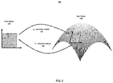
- the latent variable of a point x in the input space 110 may be approximated by the inference network (encoder) h 120.
- the inference network (encoder) h 120 Given an ⁇ and a full rank J f ( z ) at z and ⁇ , f is locally invertible in the open neighborhood f ( S ), S being an open neighborhood of z.
- a goal is to learn an h : f ( S ) ⁇ S such that E ⁇ ⁇ N 0 I D h f z ⁇ z , ⁇ z ⁇ S .
- z ) is parametric with the extended generator f .
- a constraint is added to Eq.
- x ) is a Gaussian distribution with the sample average of h ( x ) as the mean, and the sample standard deviation of h ( x ), x ⁇ p data ( x ) as the standard deviation.
- the objective formulae are different from a typical VAE model.
- x ) is not modeled in order to reduce model complexity.
- an objective is to learn a variance network ⁇ for the generator g rather than the decoder in VAEs.
- f follows a Gaussian Process with g as the mean function, and ⁇ ⁇ as the covariance function, and ⁇ ⁇ is a diagonal matrix with ⁇ along the diagonal.
- the learning of both networks is integrated with the training of GANs.
- the following objective may be used to adjust the generator g and h : min g , h E z ⁇ p z ⁇ z ⁇ h g z ⁇ 2 .
- FIG. 1 shows the scheme of the g and h , in which the generator network 115 maps from the latent space 105 to the input space 110 and the inference network 120 maps to the latent space 105.
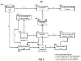
- FIG. 2 depicts a system architecture 200, according to embodiments of the present invention.
- the overall system 200 comprises four main networks: a discriminator network 210, a generator network 235, an inference network 245, and a variance network 255.
- the discriminator network 210 receives as input samples from an input data set 205, which may be, for example, real image or other types of data, and generated data 225, which is generated by the generator network 235.
- the generator network 235 receives as inputs data from a prior for the latent variable ( z ) 230 and latent variables ( ⁇ ) 250.
- the inference network 245 receives as inputs data from the input data set 205 and data from the generator network 235, and outputs the latent variables ( ⁇ ) 250 and data for loss computation 220.
- the variance network 255 receives latent variables 250 from the inference network 245 and provides output to compute losses for the inference and variance networks 240.
- paths labeled with a, b, and/or c which indicate paths for losses.
- Paths labeled with "a” are related to loss for the discriminator and generator networks.
- Paths labeled with "b” are related to loss for the inference and variance networks.
- paths labeled with "c” are related to loss for the inference and generator networks.
- a methodology to learn the inference network h and the variance network ⁇ may be combined with the learning of the generator network g and the discriminator network d in a GAN.
- An embodiment of a training procedure is given in Methodology 1 (below).
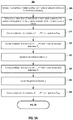
- FIGS. 3A and 3B depicts a methodology for training, according to embodiments of the present disclosure.
- a fixed number of hidden variables are sampled (305) from a hidden variable prior for K -means clustering.
- K clusters are computed (310), in which each cluster, k, has a center c k , a number of data points in the cluster ( C k ), and a parameter ( ⁇ k ) (see Section B.1.) for the variance neural network.
- a minibatch of m samples ⁇ x (1) , ..., x ( m ) ⁇ is obtained by sampling (315) from input data (e.g., P data ), and a minibatch of m samples ⁇ z ( 1 ) , ..., z ( m ) ⁇ is obtained by sampling (320) from a hidden variable prior (e.g., ).
- the discriminator network is updated (325).
- a minibatch of m samples ⁇ z (1) , ..., z ( m ) ⁇ is obtained by sampling (330) from a hidden variable prior (e.g., ).
- the generator network is updated (335).
- a minibatch of m samples ⁇ x (1) , ..., x ( m ) ⁇ is obtained by sampling (340) from input data (e. g., P data ).
- input data e. g., P data
- the inference network, h, and the variance network, ⁇ are updated (345).
- a minibatch of m samples ⁇ z (1) , ..., z ( m ) ⁇ is obtained by sampling from the hidden variable prior.
- the inference network and the generator network are updated (355).
- a stop condition may include: (1) a set number of iterations have been performed; (2) an amount of processing time has been reached; (3) convergence (e.g., the difference in a loss or losses (or a gradient or gradients) between consecutive iterations are less than a threshold value; (4) divergence (e.g., the performance begins to deteriorate); and (5) an acceptable loss or losses have been reached.
- the trained networks may be output (e.g, the generator network ( g ), the discriminator network (d), the inference network (h), and the variance network ( ⁇ )).
- Lemma 3 regards the updating steps for W .
- Methodology 1 also avoids the step to directly fit the parameters of generator g with real data samples, and thus can preserve the capability of GAN to generate sharp and realistic images or data samples.
- W t be the matrix W at the updating step t of Methodology 1, then W t +1 will be the element-wise multiplication of W t with another matrix.
- W t With a batch of training samples , W t will be the element-wise product of W t -1 with an aggregated updating matrix, which is
- W 0 be the initial value of W
- the final step W T will be the element-wise multiplication of W 0 with the aggregated updating matrix regarding all steps.
- W 0 is randomly initialized and the updating matrix is almost with full rank due to the randomness of training samples.
- the time-consuming part may be the computation of the likelihood in the testing stage, which is due to the calculation of J g , and g is a mapping from dim(Z) to dim(X).
- Methodology 1 basically follows the same procedure to learn the generator g and the discriminator d in GANs.
- the only interaction between g and h is to enhance the mutual information between latent variables and the generated samples.
- the loss functions for d and g may be adapted to any other forms of divergence to measure distribution distances, such as Wasserstein distance.
- Wasserstein distance Without loss generality, presented herein is a study of the theoretical upper bound of distribution estimation with the approach presented in this patent document. Existing approaches may be followed to analysis the estimation upper bound.
- the definition of Earth Moving Distance, or equivalently Wasserstein-1 distance may be adopted.
- THEOREM 1 Let be certain function class and g : R d ⁇ R D be an L-Lipschitz function for D > d > 2 .
- Z be random variable satisfying E ⁇ Z ⁇ 2 ⁇ c and be the distribution of g ( Z ).
- PROOF Let , and be the distribution of g ( Z ) + ⁇ , g ( Z ) , and ⁇ ( Z ) respectively.
- W P P 1 n inf ⁇ ⁇ ⁇ P 1 P 1 n E X Y ⁇ ⁇ ⁇ X ⁇ Y ⁇ ⁇ inf ⁇ ⁇ ⁇ Q Q n E X Y ⁇ ⁇ ⁇ g X ⁇ g Y ⁇ ⁇ inf ⁇ ⁇ ⁇ Q Q n E X Y ⁇ ⁇ L ⁇ X ⁇ Y ⁇ ⁇ LW Q Q n .
- ⁇ be the optimal joint distribution for the infimum of W P 1 Q . It is noted that ⁇ does not necessarily exists in general. However, for every ⁇ > 0, there exists ⁇ ⁇ ⁇ ⁇ P 1 Q such that: W P 1 Q + ⁇ ⁇ E X Y ⁇ ⁇ ⁇ ⁇ X ⁇ Y ⁇ .
- ⁇ the joint distribution of ( X, Y ) such that Y ⁇ Q and X
- LEMMA 5 Let and be distributions on . Let and be the empirical distribution of and , respectively. Then: E W P n , P n + Q n ⁇ E X ⁇ Q ⁇ X ⁇ .
- PROOF PROOF.
- THEOREM 2 (THEOREM 1 in the Fournier and Guillin document referenced above) Let be distribution on and be its n-sample empirical distribution. Suppose E X ⁇ P ⁇ X ⁇ 2 ⁇ c , then E W P P n ⁇ C d c n ⁇ d ,
- an embodiment of the likelihood estimation methodology is first evaluated with various data sets. Then, an embodiment of the methodology is applied to anomaly detection tasks.
- “InvGAN” is used to represent an embodiment or embodiments of the present patent document. The implementation of the InvGAN embodiment or embodiments used in testing were based on the PaddlePaddle platform.
- FlowGAN is a hybrid model with maximum likelihood estimation (MLE) and adversarial loss. They employ coupling layers (as proposed in Laurent Dinh, Jascha Sohl-Dickstein, and Samy Bengio, "Density estimation using Real NVP," in 5th International Conference on Learning Representations (ICLR), Toulon, France (2017 )) for the generator. With the coupling layers, the generator has the same number of dimensions for both latent space and input space. With the coupling layers, the determinate of the generator can be easily computed, and thus the likelihood of the samples. FlowGAN trains the generator based on both MLE and the adversarial the loss functions.
- a FlowVAE model was built with the decoder that had the same structure as the generator in the FlowGAN model.
- the InvGAN embodiment and the FlowGAN model had the sample structure for the discriminator, which includes four linear layers and three Relu layers. The same batch size and epoch number was used to train the three models.
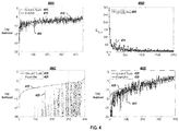
- FIG. 4 gives the comparison between the ground truth and the estimated likelihood values for the testing set with three methods, according to embodiments of the present disclosure.
- the upper left plot 400A shows the InvGAN embodiment log-likelihoods of the simulated testing set; the upper right plot 400B presents the objective loss values over iterations; the lower two plots (400C and 400D) give the log-likelihood values of the simulated data set using FlowVAE and FlowGAN.
- the Y-axis is the log-likelihood value, and the X-axis is sample index based on the increasing order of the ground truth log-likelihood value. It can be seen that compared with FlowGAN and FlowVAE, the tested embodiment can give more smooth estimations for the likelihood values, and improved fitting with the ground truth likelihood curve.
- FIG. 5 depicts a method for likelihood estimation, according to embodiments of the present disclosure.
- the depicted method uses (505) a set of input data and three trained networks-a trained generator network ( g ), a trained inference network ( h ), and trained variance network ( ⁇ ).
- the trained inference network ( h ) is used to obtain (510) a set of hidden variables ( z ) corresponding to the set of input data.
- the set of hidden variables are input (515) into the trained generator network ( g ) and the trained variance network ( ⁇ ).
- a set of Riemannian metric matrices may then be computed (520) using a Jacobian matrix or matrices for the trained generator network ( g ) and the trained variance network ( ⁇ ) regarding the set of hidden variables.
- log-likelihood values for the set of input data may be computed (525) using the set of Riemannian metric matrices and the log-likelihood values of the set of hidden variables Table 1: Bits/dim on testing data sets for different models; lower is better Model Data Set 1 Data Set 2 Data Set 3 RealNVP 1.06 3.49 4.28 Glow 1.05 3.35 4.09 FFJORD 0.99 3.40 - MADE 2.04 5.67 - MAF 1.89 4.31 - FlowGAN 3.26 4.21 - InvGAN 1.29 1.23 1.02
- the tested embodiment was compared with the other likelihood estimation methods using three data sets.
- the methods listed in the Table 1 include RealNVP, Glow, FFJord, FlowGAN, MADE, and MAF ( George Papamakarios, Iain Murray, and Theo Pavlakou, "Masked Autoregressive Flow for Density Estimation," in Advances in Neural Information Processing Systems (NIPS). Long Beach, CA, 2338-2347 (2017 )). Most of these methods are based on maximum likelihood estimation (MLE).
- MLE maximum likelihood estimation
- FlowGAN is a hybrid model combining MLE and adversarial loss. RealNVP, Glow, and FlowGAN rely on revertible coupling layers to preserve the density mass between the input space to latent space.
- MADE and MAF are mask-based neural density estimation methods.
- three convolution layers and one linear layer were used for the generator, the discriminator, and the inference network. More details about the network structures are given in Appendix A.
- FIG. 6 presents, in a first plot 600A, the average negative log-likelihood values of Data set 1 testing data using the InvGAN embodiment at different latent space dimension (d) 600A, according to embodiments of the present disclosure.
- the bits-per-dimension metric i.e., -log p x ( x )/ D, x ⁇ R D , may not apply to the tested embodiment model, as the tested embodiment yields the smallest bits/dim value due the small latent space dimension number used in the model.
- bits-per-dimension metric was used in the comparison, which is
- d is the latent space dimension size.
- the bits/dim of the InvGAN embodiment can be bounded in a reasonable range (as shown the bottom plot 600B of FIG. 6).
- FIG. 6 presents, in a second plot 600B, the corresponding bits/dim for the testing set under the revised metric at different d value, according to embodiments of the present disclosure.
- the new metric can compensate the difference resulted from different latent space dimension numbers.
- the experimental setup in FFJord and FlowGAN was followed, and
- Table 1 compares different methods under the new metric on testing data sets. The likelihood values presented in FFJord and FlowGAN were used. It can be seen that even with the revised metric, the tested embodiment model consistently performed better compared with other models.
- FIG. 7 depicts a method for anomaly detection, according to embodiments of the present disclosure.
- a method like that of FIGS. 3A-B may be used to train (705) the networks.
- a method like that of FIG. 5 may be used to obtain (710) log-likelihood values.
- the log-likelihood values are used (715) to compute anomaly scores for the set of test data, and responsive to an anomaly score not exceeding a threshold value, the test data sample may be designated (720) as being an anomaly.
- Table 2 Statistics of the data sets for anomaly detection Data Set Feature Instance Data set 1 ⁇ 1,000 60,000 Data set 2 ⁇ 3,000 60,000 Data set 3 ⁇ 274 ⁇ 450
- a likelihood estimation embodiment is used for three anomaly detection tasks. Table 2 gives more details on the three data sets.
- DSEBM Deep Structured Energy Based Models
- ICML Machine Learning
- New York, NY, 1100-1109 (2016 ) are energy-based models for anomaly detection. Similar to denoising auto-encoder, the main idea is to accumulate the energy across layers of neural networks. Two types of anomaly scoring criteria were proposed: energy-based and reconstruction error-based. In the experimental results, DSEBM-r represents results with reconstruction error and DSEBM-e are results with energy-based approach.
- DAGMM Deep Autoencoding Gaussian Mixture Model
- ICLR International Conference on Learning Representations
- AnoGAN ( Thomas Schlegl, Philipp Seeböck, Sebastian M. Waldstein, Ursula Schmidt-Erfurth, and Georg Langs, "Unsupervised Anomaly Detection with Generative Adversarial Networks to Guide Marker Discovery," in Proceedings of 25th International Conference on Information Processing in Medical Imaging (IPMI).
- Boone, NC, 146-157 (2017 ) is a GAN-based method for anomaly detection.
- the method trains a GAN model to recover a latent representation for each test data sample.
- the anomaly score is calculated with a combination of the reconstruction error and the discrimination score from the discriminator network.
- the reconstruction error measures how well the GAN can reconstruct the data via the inferred latent variable and the generator.
- the authors of AnoGAN compare the two components for the anomaly score and the variant which performed best in the paper was selected.
- EGBAD Efficient GAN-Based Anomaly Detection
- GANomaly uses a conditional generative adversarial network that jointly learns the generation of high-dimensional image space and the inference of latent space.
- Employing encoder-decoder-encoder sub-networks in the generator enables the model to map the input image to a lower dimension vector, which is then used to reconstruct the generated output image.
- the use of the additional encoder network maps this generated image to its latent representation. Minimizing the distance between these images and the latent vectors during training aids in learning the effective representations for the normal samples.
- Adversarially Learned Anomaly Detection ( Houssam Zenati, Manon Romain, Chuan-Sheng Foo, Bruno Lecouat, and Vijay Chandrasekhar, "Adversarially Learned Anomaly Detection," in IEEE International Conference on Data Mining (ICDM). Singapore, 727-736 (2018 )) is a recently proposed GAN-based anomaly detection method. Similar to EGBAD ( Shuangfei Zhai, Yu Cheng, Weining Lu, and Zhongfei Zhang, “Deep Structured Energy Based Models for Anomaly Detection," in Proceedings of the 33nd International Conference on Machine Learning (ICML).
- ALAD learns an encoding function to infer the latent variable for testing samples.
- Their model is enhanced with three discriminators. With a cycle consistence between sample space and latent space, the training of their model can be stabilized in learning representations for anomaly detection.
- OC-SVM Class Support Vector Machines
- OC-SVM Bernhard Schölkopf, Robert C. Williamson, Alexander J. Smola, John Shawe-Taylor, and John C. Platt, "Support Vector Method for Novelty Detection," in Advances in Neural Information Processing Systems (NIPS).
- NIPS Neural Information Processing Systems
- Denver, CO, 582-588 (1999 ) are a classic kernel method for anomaly detection and density estimation that learns a decision boundary around normal examples.
- the radial basis function (RBF) kernel is employed in the experiments.
- the ⁇ parameter is set to the expected anomaly proportion in the data set, which is assumed to be known, whereas the ⁇ parameter is set to be inversely proportional to the number of input features.
- Isolation Forests Fei Tony Liu, Kai Ming Ting, and Zhi-Hua Zhou, "Isolation Forest," in Proceedings of the 8th IEEE International Conference on Data Mining (ICDM). Pisa, Italy, 413-422 (2008 )
- IF Isolation Forests
- the method constructs trees across randomly chosen features according to randomly split values.
- the anomaly score is defined as the average path length from a testing sample to the root. The experiments results for this model were obtained with the implementation in the scikit-learn package.
- One class of the ten numbers in Data set 1 were taken as the abnormal class, and the rest classes were taken as the normal class.
- the images from the nine normal classes were to train GAN and an embodiment of the present disclosure.
- the testing state the images from all ten classes in the testing set were used.
- the experiment set up followed GANomaly.
- the results for GANomaly were obtained by running the online code with the optimal parameters given in the script.
- the results for the other methods were based on the result section in GANomaly, referenced above.
- the upper plot 800A in FIG. 8 shows the results of all of the methods on ten classes.
- Table 3 Anomaly detection on Data set 1 and Data set 2 Data Set Model AUROC DATA SET 1 VAE 0.3420 ⁇ 0.1861 AnoGAN 0.4390 ⁇ 0.116 GANomaly 0.7390 ⁇ 0.0882 InvGAN 0.7920 ⁇ 0.0786 DATA SET 2 OC-SVM* 0.5843 ⁇ 0.0956 IF* 0.6025 ⁇ 0.1040 DSEBM-r* 0.6071 ⁇ 0.1007 DSEBM-e* 0.5956 ⁇ 0.1151 ALAD* 0.6072 ⁇ 0.1201 AnoGAN 0.5949 ⁇ 0.1076 EGBAD 0.4450 ⁇ 0.0786 GANomaly 0.6065 ⁇ 0.0390 InvGAN 0.6391 ⁇ 0.0608
- Table 3 presents comparison among different anomaly detection methods for both image data sets.
- the experimental setups for AnoGAN, EGBAD, GANomaly, and the proposed InvGAN were the same and follow the GANomaly document, cited above.
- some anomaly detection results for Data set 2 were also included.
- FIG. 9 gives the convergence of the loss L h, ⁇ for different data sets: 900A (Data set 1), 900B (Data set 2), 900C (Data set 3), and 900D (Data set 4).
- Table 4 Anomaly detection on Data set 4 Data Set Model Precision Recall F1 Score Data set 4 OC-SVM 0.5397 0.4082 0.4581 IF 0.5147 0.5469 0.5303 DSEBM-r 0.1515 0.1513 0.1510 DSEBM-e 0.4667 0.4565 0.4601 DAGMM 0.4909 0.5078 0.4983 AnoGAN 0.4118 0.4375 0.4242 ALAD 0.5000 0.5313 0.5152 InvGAN 0.4390 0.6000 0.5070
- embodiments of an approach to estimate the implicit likelihoods of GANs were presented.
- the likelihoods of testing samples can be estimated.
- Simulation study and likelihood testing on data sets validate the advantages of embodiments.
- An embodiment was further applied to three anomaly detection tasks. Experimental results show that the tested embodiment can outperform classic and other deep neural network-based anomaly detection methods.
- Table 5 Generator of InvGAN in likelihood and anomaly detection experiments for Data set 1 and Data set 2
- Table 5 Generator Layer Number of Output Kernel Stride Activation function Input z ⁇ N(0,1) 50 50 Fully-Connected 128 ⁇ 4 ⁇ 4 ReLU Transposed convolution 128 ⁇ 8 ⁇ 8 4 ⁇ 4 2 ReLU Transposed convolution 64 ⁇ 16 ⁇ 16 4 ⁇ 4 2 ReLU Transposed convolution 1 ⁇ 32 ⁇ 32 (Data set 1) 4 ⁇ 4 2 Tanh 3 ⁇ 32 ⁇ 32 (Data set 2) 4 ⁇ 4 2 Tanh Table 6: Discriminator of the InvGAN embodiment in likelihood and anomaly detection experiments for Data set 1 and Data set 2 Discriminator Layer Number of Output Kernel Stride Activation function Input x 1 ⁇ 32 ⁇
- Table 8 Generator of the InvGAN embodiment in Data set 4 anomaly detection experiments Generator Layer Number of Output Batch Normalization Activation function Input z ⁇ N (0,1) z dim 50 Fully-Connected 128 Y ReLU Fully-Connected 256 Y ReLU Fully-Connected 274
- Table 9 Discriminator of the InvGAN embodiment in Data set 4 anomaly detection experiments Discriminator Layer Number of Output Batch Normalization Activation function Input x 274 Fully-Connected 256 Y ReLU Fully-Connected 128 Y ReLU Fully-Connected 1 Sigmoid Table 10: Inference network of the InvGAN embodiment in Data set 4 anomaly detection experiments Inference Network Layer Number of Output Batch Normalization Activation function Input x 274 Fully-Connected 256 Y ReLU Fully-Connected 128 Y ReLU Fully-Connected 50
- aspects of the present patent document may be directed to, may include, or may be implemented on one or more information handling systems/computing systems.
- a computing system may include any instrumentality or aggregate of instrumentalities operable to compute, calculate, determine, classify, process, transmit, receive, retrieve, originate, route, switch, store, display, communicate, manifest, detect, record, reproduce, handle, or utilize any form of information, intelligence, or data.
- a computing system may be or may include a personal computer (e.g., laptop), tablet computer, phablet, personal digital assistant (PDA), smart phone, smart watch, smart package, server (e.g., blade server or rack server), a network storage device, camera, or any other suitable device and may vary in size, shape, performance, functionality, and price.
- the computing system may include random access memory (RAM), one or more processing resources such as a central processing unit (CPU) or hardware or software control logic, ROM, and/or other types of memory.
- Additional components of the computing system may include one or more disk drives, one or more network ports for communicating with external devices as well as various input and output (I/O) devices, such as a keyboard, a mouse, touchscreen and/or a video display.
- the computing system may also include one or more buses operable to transmit communications between the various hardware components.
- FIG. 10 depicts a simplified block diagram of a computing device/information handling system (or computing system) according to embodiments of the present disclosure. It will be understood that the functionalities shown for system 1000 may operate to support various embodiments of a computing system-although it shall be understood that a computing system may be differently configured and include different components, including having fewer or more components as depicted in FIG. 10 .
- the computing system 1000 includes one or more central processing units (CPU) 1001 that provides computing resources and controls the computer.
- CPU 1001 may be implemented with a microprocessor or the like, and may also include one or more graphics processing units (GPU) 1019 and/or a floating-point coprocessor for mathematical computations.
- System 1000 may also include a system memory 1002, which may be in the form of random-access memory (RAM), read-only memory (ROM), or both.
- RAM random-access memory
- ROM read-only memory
- An input controller 1003 represents an interface to various input device(s) 1004, such as a keyboard, mouse, touchscreen, and/or stylus.
- the computing system 1000 may also include a storage controller 1007 for interfacing with one or more storage devices 1008 each of which includes a storage medium such as magnetic tape or disk, or an optical medium that might be used to record programs of instructions for operating systems, utilities, and applications, which may include embodiments of programs that implement various aspects of the present disclosure.
- Storage device(s) 1008 may also be used to store processed data or data to be processed in accordance with the disclosure.
- the system 1000 may also include a display controller 1009 for providing an interface to a display device 1011, which may be a cathode ray tube (CRT), a thin film transistor (TFT) display, organic light-emitting diode, electroluminescent panel, plasma panel, or other type of display.
- a display controller 1009 for providing an interface to a display device 1011, which may be a cathode ray tube (CRT), a thin film transistor (TFT) display, organic light-emitting diode, electroluminescent panel, plasma panel, or other type of display.
- the computing system 1000 may also include one or more peripheral controllers or interfaces 1005 for one or more peripherals 1006. Examples of peripherals may include one or more printers, scanners, input devices, output devices, sensors, and the like.
- a communications controller 1014 may interface with one or more communication devices 1015, which enables the system 1000 to connect to remote devices through any of a variety of networks including the Internet, a cloud resource (e.g., an Ethernet cloud, a Fiber Channel over Ethernet (FCoE)/Data Center Bridging (DCB) cloud, etc.), a local area network (LAN), a wide area network (WAN), a storage area network (SAN) or through any suitable electromagnetic carrier signals including infrared signals.
- a cloud resource e.g., an Ethernet cloud, a Fiber Channel over Ethernet (FCoE)/Data Center Bridging (DCB) cloud, etc.
- FCoE Fiber Channel over Ethernet
- DCB Data Center Bridging
- LAN local area network
- WAN wide area network
- SAN storage area network
- electromagnetic carrier signals including infrared signals.
- bus 1016 which may represent more than one physical bus.
- various system components may or may not be in physical proximity to one another.
- input data and/or output data may be remotely transmitted from one physical location to another.
- programs that implement various aspects of the disclosure may be accessed from a remote location (e.g., a server) over a network.
- Such data and/or programs may be conveyed through any of a variety of machine-readable medium including, but are not limited to: magnetic media such as hard disks, floppy disks, and magnetic tape; optical media such as CD-ROMs and holographic devices; magneto-optical media; and hardware devices that are specially configured to store or to store and execute program code, such as application specific integrated circuits (ASICs), programmable logic devices (PLDs), flash memory devices, and ROM and RAM devices.
- ASICs application specific integrated circuits
- PLDs programmable logic devices
- flash memory devices ROM and RAM devices.
- aspects of the present disclosure may be encoded upon one or more non-transitory computer-readable media with instructions for one or more processors or processing units to cause steps to be performed.
- the one or more non-transitory computer-readable media may include volatile and/or non-volatile memory.
- alternative implementations are possible, including a hardware implementation or a software/hardware implementation.
- Hardware-implemented functions may be realized using ASIC(s), programmable arrays, digital signal processing circuitry, or the like. Accordingly, the "means” terms in any claims are intended to cover both software and hardware implementations.
- computer-readable medium or media includes software and/or hardware having a program of instructions embodied thereon, or a combination thereof.
- embodiments of the present disclosure may further relate to computer products with a non-transitory, tangible computer-readable medium that have computer code thereon for performing various computer-implemented operations.
- the media and computer code may be those specially designed and constructed for the purposes of the present disclosure, or they may be of the kind known or available to those having skill in the relevant arts.
- Examples of tangible computer-readable media include, but are not limited to: magnetic media such as hard disks, floppy disks, and magnetic tape; optical media such as CD-ROMs and holographic devices; magneto-optical media; and hardware devices that are specially configured to store or to store and execute program code, such as application specific integrated circuits (ASICs), programmable logic devices (PLDs), flash memory devices, and ROM and RAM devices.
- ASICs application specific integrated circuits
- PLDs programmable logic devices
- flash memory devices and ROM and RAM devices.
- Examples of computer code include machine code, such as produced by a compiler, and files containing higher level code that are executed by a computer using an interpreter.
- Embodiments of the present disclosure may be implemented in whole or in part as machine-executable instructions that may be in program modules that are executed by a processing device.
- Examples of program modules include libraries, programs, routines, objects, components, and data structures. In distributed computing environments, program modules may be physically located in settings that are local, remote, or both.
Landscapes
- Engineering & Computer Science (AREA)
- Theoretical Computer Science (AREA)
- Physics & Mathematics (AREA)
- Data Mining & Analysis (AREA)
- Artificial Intelligence (AREA)
- General Engineering & Computer Science (AREA)
- Evolutionary Computation (AREA)
- General Physics & Mathematics (AREA)
- Life Sciences & Earth Sciences (AREA)
- Software Systems (AREA)
- Computational Linguistics (AREA)
- Mathematical Physics (AREA)
- Computing Systems (AREA)
- Biophysics (AREA)
- Molecular Biology (AREA)
- General Health & Medical Sciences (AREA)
- Biomedical Technology (AREA)
- Health & Medical Sciences (AREA)
- Probability & Statistics with Applications (AREA)
- Bioinformatics & Cheminformatics (AREA)
- Bioinformatics & Computational Biology (AREA)
- Computer Vision & Pattern Recognition (AREA)
- Evolutionary Biology (AREA)
- Management, Administration, Business Operations System, And Electronic Commerce (AREA)
- Complex Calculations (AREA)
- Debugging And Monitoring (AREA)
Abstract
Description
- The present disclosure relates generally to systems and methods for computer learning that can provide improved computer performance, features, and uses. More particularly, the present disclosure relates to embodiments for estimating the implicit likelihoods of generative adversarial networks (GANs).
- Many real-world high dimensional data sets concentrate around low dimensional unknown manifolds. Deep models provide new approaches to estimate the density of extreme high dimensional data. Generative models, e.g., generative adversarial networks (GANs), can learn the distributions of high dimensional data sets and generate samples as well. GANs typically use the adversarial loss as their training objective, which penalizes dissimilarity between the distribution of the generated samples and the real samples. Given infinite approximation power, the original GAN objectives aim to minimize the Jensen-Shannon divergence between the real data distribution and generated samples.
- The generator in a GAN can be seen as a nonlinear parametric mapping

- Due to the broad applications of GANs, it is important to measure the distribution likelihoods of any given samples. However, GANs are implicit models, which means that the sample likelihoods cannot be computed directly. The discriminator used in the GAN is designed to classify the samples from true data distribution and the samples from the generator. Thus, the discriminator cannot estimate the likelihoods of the samples that do not belong to either distributions. It has been proven that there exists an inverse function of the generator that can project samples in the sample space into the latent space. An approach has been provided by Aditya Ramesh and Yann LeCun in "Backpropagation for Implicit Spectral Densities," Technical Report (2018) (available at arXiv.org/pdf/1806.00499.pdf) to estimate the spectral implicit density of generative models. However, this method does not provide a qualitative way to estimate the likelihood of any given samples.
- Accordingly, what is needed are approaches that can learn an inverse function of the generator of GAN models that preserve the measurement consistence.
- The present disclosure provides a computer-implemented method for training a generative adversarial network system, a computer-implemented method for likelihood estimation of data, and a computer-implemented method for anomaly detection.
- In a first aspect, a computer-implemented method for training a generative adversarial network system, comprises: responsive to a stop condition not being reached, repeating steps for training a generative adversarial network system comprising a generator network, a discriminator network, an inference network, and a variance network, the steps comprising: sampling a first minibatch of input data samples from an input data set; sampling a minibatch of hidden variable values from a hidden variable prior distribution; updating the discriminator network using first loss function; sampling a second minibatch of hidden variable values from the hidden variable prior distribution; updating the generator network using a second loss function; sampling a second minibatch of input data samples from the input data set; updating the inference network and the variance network using a third loss function; sampling a third minibatch of hidden variable values from the hidden variable prior distribution; and updating the inference network and the generator network using a fourth loss function; and responsive to a stop condition being reached, output a trained generator network, a trained inference network, and a trained variance network.
- The method further comprises the step of: obtaining a plurality of clusters of hidden variable values by sampling a number of hidden variable values from the hidden variable prior distribution and using K-means clustering to obtain the plurality of clusters.
- The step of updating the inference network comprises: training the inference network to map a given input data sample in an input space to a hidden variable value that can be mapped back to a value within a region of the input data sample in a manifold.
- The third loss function comprises: a difference between the generator network estimate of an input data sample using as an input the estimate of a hidden variable value obtained using the inference network and the input data sample.
- The third loss function further comprises: for the input data sample, determining a variance value using the variance network operating on the estimate of the hidden variable value obtained using the inference network and the input data sample.
- The fourth loss function comprises: a difference between a sampled hidden variable value and an estimate of the sampled hidden variable value obtained from the inference network using as an input an estimate of an input data sample for the sampled hidden variable, in which the estimate of the input data sample is obtained from the generator network and the sampled hidden variable value.
- In a second aspect, a computer-implemented method for likelihood estimation of data comprises: obtain a set of latent variable values corresponding to a set of input data values using a trained inference network, which has been trained to map an input data value to a latent variable value that can be mapped back to a value within a region of the input data value in a manifold using a trained generator network; inputting the set of latent variable values into the trained generator network and a trained variance network, which has been trained to map a latent variable to a variance value that captures a local regional uncertainty in an input space; determining a set of Riemannian metric matrices using one or more Jacobian matrices for the trained generator network and the trained variance network regarding the set of latent variable values; and determining log-likelihood values for the set of input data values using the set of Riemannian metric matrices and log-likelihood values of the set of hidden variable values.
- The trained generator network, the trained inference network, and the trained variance network were obtained by training a Generative Adversarial Network (GAN) system that comprised the generator network, the inference network, and the variance network.
- The step of training the GAN system that comprises the generator network, the inference network, and the variance network comprises the steps of: responsive to a stop condition not being reached, repeating steps for training the GAN system comprising the generator network, a discriminator network, the inference network, and the variance network, the steps comprising: sampling a first minibatch of input data samples from an input data set; sampling a minibatch of latent variable values from a latent variable prior distribution; updating the discriminator network using first loss function; sampling a second minibatch of latent variable values from the latent variable prior distribution; updating the generator network using a second loss function; sampling a second minibatch of input data samples from the input data set; updating the inference network and the variance network using a third loss function; sampling a third minibatch of latent variable values from the latent variable prior distribution; and updating the inference network and the generator network using a fourth loss function; and responsive to a stop condition being reached, output a trained generator network, a trained inference network, and a trained variance network.
- The method further comprises: obtaining a plurality of clusters of latent variable values by sampling a number of latent variable values from the latent variable prior distribution and using K-means clustering to obtain the plurality of clusters.
- The third loss function comprises: a difference between the generator network estimate of an input data sample using as an input the estimate of a latent variable value obtained using the inference network and the input data sample.
- The third loss function further comprises: for the input data sample, determining a variance value using the variance network operating on the estimate of the latent variable value obtained using the inference network and the input data sample.
- The fourth loss function comprises: a difference between a sampled latent variable value and an estimate of the sampled latent variable value obtained from the inference network using as an input an estimate of an input data sample for the sampled latent variable, in which the estimate of the input data sample is obtained from the generator network and the sampled latent variable value.
- In a third aspect, a computer-implemented method for anomaly detection comprises: obtain a set of latent variable values corresponding to a set of input data values using a trained inference network, which has been trained to map an input data value to a latent variable value that can be mapped back to a value within a region of the input data value in a manifold using a trained generator network; inputting the set of latent variable values into the trained generator network and a trained variance network, which has been trained to map a latent variable to a variance value that captures a local regional uncertainty in an input space; determining a set of Riemannian metric matrices using one or more Jacobian matrices for the trained generator network and the trained variance network regarding the set of latent variable values; and determining log-likelihood values for the set of input data values using the set of Riemannian metric matrices and log-likelihood values of the set of hidden variable values; using at least some of the log-likelihood values to determine corresponding anomaly scores corresponding to the set of input data values; and responsive to an anomaly score not exceeding a threshold value, designating the input data value corresponding to the anomaly score as being an anomaly.
- The trained generator network, the trained inference network, and the trained variance network were obtained by training a Generative Adversarial Network (GAN) system that comprised the generator network, the inference network, and the variance network.
- The step of training the GAN system that comprises the generator network, the inference network, and the variance network comprises the steps of: responsive to a stop condition not being reached, repeating steps for training the GAN system comprising the generator network, a discriminator network, the inference network, and the variance network, the steps comprising: sampling a first minibatch of input data samples from an input data set; sampling a minibatch of latent variable values from a latent variable prior distribution; updating the discriminator network using first loss function; sampling a second minibatch of latent variable values from the latent variable prior distribution; updating the generator network using a second loss function; sampling a second minibatch of input data samples from the input data set; updating the inference network and the variance network using a third loss function; sampling a third minibatch of latent variable values from the latent variable prior distribution; and updating the inference network and the generator network using a fourth loss function; and responsive to a stop condition being reached, output a trained generator network, a trained inference network, and a trained variance network.
- The method further comprises: obtaining a plurality of clusters of latent variable values by sampling a number of latent variable values from the latent variable prior distribution and using K-means clustering to obtain the plurality of clusters.
- The third loss function comprises: a difference between the generator network estimate of an input data sample using as an input the estimate of a latent variable value obtained using the inference network and the input data sample.
- The third loss function further comprises: for the input data sample, determining a variance value using the variance network operating on the estimate of the latent variable value obtained using the inference network and the input data sample.
- The fourth loss function comprises: a difference between a sampled latent variable value and an estimate of the sampled latent variable value obtained from the inference network using as an input an estimate of an input data sample for the sampled latent variable, in which the estimate of the input data sample is obtained from the generator network and the sampled latent variable value.
- In a fourth aspect, a non-transitory machine-readable medium having instructions stored therein, which when executed by a processor, cause the processor to perform any of the methods described above.
- In a fourth aspect, a data processing system, comprising: a processor; and a memory coupled to the processor to store instructions, which when executed by the processor, cause the processor to perform any of the methods described above.
- In a fourth aspect, a computer program product having computer programs stored therein, which when executed by a processor, cause the processor to perform any of the methods described above.
- References will be made to embodiments of the disclosure, examples of which may be illustrated in the accompanying figures. These figures are intended to be illustrative, not limiting. Although the disclosure is generally described in the context of these embodiments, it should be understood that it is not intended to limit the scope of the disclosure to these particular embodiments. Items in the figures may not be to scale.
- Figure ("
FIG.") 1 graphically depicts learning an approximate inverse (inference) function of the generator network, according to embodiments of the present disclosure. -
FIG. 2 depicts an examples system architecture for training, according to embodiments of the present invention. -
FIGS. 3A and3B depicts a methodology for training, according to embodiments of the present disclosure. -
FIG. 4 gives the comparison between the ground truth and the estimated likelihood values for the testing set with three methods, according to embodiments of the present disclosure. -
FIG. 5 depicts a method for likelihood estimation, according to embodiments of the present disclosure. -
FIG. 6 presents, in afirst plot 600A, the average negative log-likelihood values of Data set 1 testing data using the InvGAN embodiment at different latent space dimension (d), and presents, in asecond plot 600B, the corresponding bits/dim for the testing set under the revised metric at different d values, according to embodiments of the present disclosure. -
FIG. 7 depicts a method for anomaly detection, according to embodiments of the present disclosure. -
FIG. 8 depicts anomaly detection with different models onData sets -
FIG. 9 depicts Lh,σ at different iterations for the four data sets, according to embodiments of the present disclosure. -
FIG. 10 depicts a simplified block diagram of a computing device/information handling system, according to embodiments of the present disclosure. - In the following description, for purposes of explanation, specific details are set forth in order to provide an understanding of the disclosure. It will be apparent, however, to one skilled in the art that the disclosure can be practiced without these details. Furthermore, one skilled in the art will recognize that embodiments of the present disclosure, described below, may be implemented in a variety of ways, such as a process, an apparatus, a system, a device, or a method on a tangible computer-readable medium.
- Components, or modules, shown in diagrams are illustrative of exemplary embodiments of the disclosure and are meant to avoid obscuring the disclosure. It shall also be understood that throughout this discussion that components may be described as separate functional units, which may comprise sub-units, but those skilled in the art will recognize that various components, or portions thereof, may be divided into separate components or may be integrated together, including integrated within a single system or component. It should be noted that functions or operations discussed herein may be implemented as components. Components may be implemented in software, hardware, or a combination thereof.
- Furthermore, connections between components or systems within the figures are not intended to be limited to direct connections. Rather, data between these components may be modified, re-formatted, or otherwise changed by intermediary components. Also, additional or fewer connections may be used. It shall also be noted that the terms "coupled," "connected," or "communicatively coupled" shall be understood to include direct connections, indirect connections through one or more intermediary devices, and wireless connections.
- Reference in the specification to "one embodiment," "preferred embodiment," "an embodiment," or "embodiments" means that a particular feature, structure, characteristic, or function described in connection with the embodiment is included in at least one embodiment of the disclosure and may be in more than one embodiment. Also, the appearances of the above-noted phrases in various places in the specification are not necessarily all referring to the same embodiment or embodiments.
- The use of certain terms in various places in the specification is for illustration and should not be construed as limiting. A service, function, or resource is not limited to a single service, function, or resource; usage of these terms may refer to a grouping of related services, functions, or resources, which may be distributed or aggregated.
- The terms "include," "including," "comprise," and "comprising" shall be understood to be open terms and any lists the follow are examples and not meant to be limited to the listed items. A "layer" may comprise one or more operations. The words "optimal," "optimize," "optimization," and the like refer to an improvement of an outcome or a process and do not require that the specified outcome or process has achieved an "optimal" or peak state.
- Any headings used herein are for organizational purposes only and shall not be used to limit the scope of the description or the claims. Each reference/document mentioned in this patent document is incorporated by reference herein in its entirety.
- Furthermore, one skilled in the art shall recognize that: (1) certain steps may optionally be performed; (2) steps may not be limited to the specific order set forth herein; (3) certain steps may be performed in different orders; and (4) certain steps may be done concurrently.
- It shall be noted that any experiments and results provided herein are provided by way of illustration and were performed under specific conditions using a specific embodiment or embodiments; accordingly, neither these experiments nor their results shall be used to limit the scope of the disclosure of the current patent document.
- Presented herein are embodiments of approaches that can learn an inverse function of the generator of GAN models that preserve the measurement consistence, and then apply the inverse function to data sample likelihood estimation. In the following sections, some manifold concepts for deep generative models are reviewed, and then neural network models for density estimation are introduced. Also presented is a short survey on the application of generative models to anomaly detection.
- Recently, people have tried to apply manifold analysis to generative models. For example, some have attempted to improve GAN-based semi-supervised learning by adding manifold invariant into the classifier. Others have tried to perform geodesic clustering with deep generative models. Yet others have added stochastic variables to the variational autoencoder (VAE) generator. With the variance network, the metric estimation on the data manifold can be improved. Mathematically, a deterministic generative model x = g(z) may be seen as a surface model if the generator g is sufficiently smooth.
- Provided herein is a brief review of some basic concepts on surfaces. A deep generative model represents an embedding function,


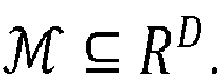 is an embedded manifold. The Jacobian of g at


 at x = g(z), denoted as
 is close to the true data manifold, namely
 .
.
- The Riemannian metric may be represented as a symmetric, positive definite matrix field, M(z), defined at each point z on the latent coordinate space,. M(z) may be given by the following formula:


- Given two tangent vectors


- where γ̇(t) is the first order derivative of γ at time t. For example, with the explicit formula of geodesic distance, one can then apply geodesic clustering on the data manifold.
- When
 to the submanifold
 of
of . It says that:

- where it is assumed that the prior distribution on the latent space pz is N(0, I d ) throughout this patent document. For


- For a real-world data set, typically one would not know the true tangent space dimension number ofat a given data sample x. People usually set

 for all x. This leads to the problem that J g does not have a full rank, and so does M(z). It means that it may be impossible to directly apply Eq. (1) with logarithm of zero determinant to estimate the sample density.
- Along with the thriving of deep neural networks and GANs, a number of density estimation methods have been developed. The MADE model (Mathieu Germain, Karol Gregor, Iain Murray, and Hugo Larochelle, "MADE: Masked Autoencoder for Distribution Estimation," in Proceedings of the 32nd International Conference on Machine Learning (ICML). Lille, France, 881-889 (2015)) was proposed to estimate the likelihood values with masked neural networks. RealNVP (Laurent Dinh, Jascha Sohl-Dickstein, and Samy Bengio, "Density estimation using Real NVP," in 5th International Conference on Learning Representations (ICLR). Toulon, France (2017)) and Glow (Diederik P. Kingma and Prafulla Dhariwal, "Glow: Generative Flow with )) are generative models that state that they can estimate samples' likelihood values. Both RealNVP and Glow employ reversible neural networks with special Jacobian metric whose determinate can be easily be calculated. Similar to RealNVP and Glow, FFJord (Will Grathwohl, Ricky T. Q. Chen, Jesse Bettencourt, Ilya Sutskever, and David Duvenaud, "FFJORD: Free-Form Continuous Dynamics for Scalable Reversible Generative Models," in 7th International Conference on Learning Representations (ICLR). New Orleans, LA (2019)) is a generative model, which can yield sample likelihood values with free-form Jacobian reversible neural network. FlowGAN (Aditya Grover, Manik Dhar, and Stefano Ermon, "FlowGAN: Combining Maximum Likelihood and Adversarial Learning in Generative Models," in Proceedings of the Thirty-Second AAAI Conference on Artificial Intelligence (AAAI). New Orleans, LA, 3069-3076. (2018)) estimates data distribution by combining maximum likelihood estimation (MLE) and adversarial loss. The combination of MLE and adversarial loss may reduce the quality of generated samples. Most of these models use flow models to avoid the singularity issues coming with GANs. However, using the same dimension number for both the latent space and the data space may violate the fact that most real-world data sets are following distributions on low dimensional manifolds. As discussed in previous subsections, GANs can approximate the real data distribution in a more reasonable approach. In this patent document, embodiments of methods are presented that can estimate the quantitative likelihood or density values of data samples by leveraging the manifold approximation power of GANs. Embodiments of the GAN likelihood estimation methodology presented herein may also be applied to anomaly detection, which (as shown herein) demonstrate their effectiveness as compared with existing anomaly detection methods. A review on anomaly detection with generative models is given in the next subsection.
- Generative models have been taken as effective ways to learn data representations and have been applied to anomaly detection. The auto-encoder based approaches first train a model that can reconstruct normal samples and then use the reconstruction errors to identify abnormal samples. Some approaches assume that the latent spaces of data sets follow Gaussian mixture distributions. Instead of utilizing auto-encoder based methods that derive statistical anomaly criterion in light of data distributions or energies, some have employed a GAN-based framework to detect abnormal medical images. In that approach, the latent variables of the samples were inferred with stochastic gradient descent. The anomaly score was estimated with the reconstruction error from the inferred latent variables in addition to the discrimination value from the discriminator of GAN model. Different from these existing methods, the new anomaly detection methodology embodiments herein are based on the proposed GAN likelihood estimation.
- In summary, presented herein are embodiments of a framework that can estimate the log-likelihoods of samples by leveraging GAN models. The proposed method embodiments can approximate the local variance of any given data points with the help of two learned networks, the variance for the generator and the inference network for the latent representation. With the variance network, the singularity of the generator's Jacobian matrix can be avoided. Thus, in one or more embodiments, the likelihoods of samples can be calculated with the Riemannian metric. Experiments on several data sets reveal that, in the tasks of anomaly detection and likelihood testing, embodiments considerably outperform other baseline methods.
- GANs attempt to estimate the empirical distributions of high dimensional data sets. Given the learned generator g, and a latent variable z, the generated sample g(z)'s log-likelihood may be estimated with Eq. (1). The computation of Eq. (1) implies the full rank of g's Jacobian matrix regarding z. One may use a low dimensional latent space, i.e., a small d, to obtain a full rank Jacobian matrix for almost any
 . Then, the sample x's log-likelihood value may be computed thanks to the generator and the newly proposed variance network.
- In one or more embodiments, a variance network σ is added to the generator g, and it extends the generator to a stochastic one,

- Here g is the mean function, σ is the variance function, and ⊙ stands for element-wise multiplication. For a given ε, f is an approximation of g, and
 . It will be shown that the singularity issue of the g's Jacobian matrix can be overcome with its variance network σ. To ensure that the variances are large in the regions without or less data samples, σ may be formulated with a radial basis function (RBF) neural network (Qichao Que and Mikhail Belkin, "Back to the Future: Radial Basis Function Networks Revisited," in Proceedings of the 19th International Conference on Artificial Intelligence and Statistics (AISTATS). Cadiz, Spain, 1375-1383 (2016)). The RBF network is a trainable kernel learning function.
- Setup and training of variance network σ. In one or more embodiments, first of all, a large number of data points are sampled from the latent space, and then these data points are divided into K clusters with K-means. ck is the center of cluster k and Ck is the number of data points in cluster k. For any data sample x, to compute the corresponding variance values, the inference network h (which is introduced in the next subsection) is first used to estimate its latent variable, i.e., z = h(x). The RBF network returns the x's variance values by aggregating the distance from z to all the cluster centers with learned kernel weights. This step may be done in a prepossessing stage and it can avoid computation overhead to the main algorithm.

- In one or more embodiments, the RBF function σ function is given by,


- where a is a hyper-parameter for the kernel, and W is the network parameter to be learned from training data samples. The samples with larger distance from the cluster centers will have larger variances. In one or more embodiments, given a generator network g, the variance network weights W can be learned by minimizing the distance between f(z) and x. With the stochastic generator f and the variance function, the Riemannian metric may be written as:

- The following is a lemma for the estimation of likelihoods.
-
LEMMA 1. With
full rank 

- PROOF. We have


- Here


- The determinate of a d × d matrix,


- Remark: Note that

- Here λi , 0 ≤ i ≤ d are the eigenvalues of

- In one or more embodiments, for a given data sample x, the corresponding latent space representation z should be found before Eq. (3) and Eq. (4) are used to compute the Riemannian metric and thus the likelihood value. As shown in
FIG. 1 , a goal is to learn an approximate inverse of thegenerator network g 115, so that for

- The latent variable of a point x in the
input space 110 may be approximated by the inference network (encoder)h 120. Given an ε and a full rank J f (z) at z and ε, f is locally invertible in the open neighborhood f (S), S being an open neighborhood of z. A goal is to learn an h: f(S) → S such that
- With the variance network σ introduced in the previous subsection, one can avoid the singularity of Riemannian metric ofas long as


- Here (p(x|z)) is parametric with the extended generator f. According to Eq. (2), given a z, p(x|z) is a multivariate Gaussian distribution with mean g(z), and co-variance matrix Λ σ , and Λ σ (z) = diag(σ(z)). In one or more embodiments, a constraint is added to Eq. (5) to include the prior distribution of z into the objective, and it forces the posterior q(z|x) (z = h(x), x ∼ pdata (x)) to be close to the prior of z, p(z) (p(z) is the pz (z) in section A.2),

- In one or more embodiments, each element of the empirical distribution q(z|x) is a Gaussian distribution with the sample average of h(x) as the mean, and the sample standard deviation of h(x), x ∼ pdata (x) as the standard deviation. The objective formulae are different from a typical VAE model. In one or more embodiments, the variance of distribution q(z|x) is not modeled in order to reduce model complexity. Moreover, given the generator g, in one or more embodiments, an objective is to learn a variance network σ for the generator g rather than the decoder in VAEs. It is easy to prove that, with

-
LEMMA 2. Assuming g is a well learned generator function with GAN model, with

- PROOF. Any collection of the entries of f follows a Gaussian distribution. According to the definition of Gaussian process, f(z) follows Gaussian Process.
- By stacking f and h together, it is a regression model to reconstruct a data sample x(x∼pdata ), i.e., x̂=g(h(x))+σ(h(x))⊙ε. With the inferred latent variables and a collection of reconstructed data samples x̂∼f(h(x)), the whole framework may be considered in some respects similar to the Gaussian Process latent variable model (GP-LVM). The objective for h and σ becomes:
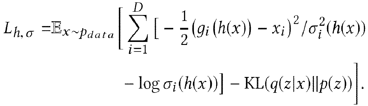
- Experimentally, it is rather difficult to learn a pair of perfect h and σ for a given g. In one or more embodiments, the learning of both networks is integrated with the training of GANs. In one or more embodiments, the following objective may be used to adjust the generator g and h:

- It may be considered similar to the regularization term in InfoGAN that enforces mutual information between the generated samples and partial latent variables. VEEGAN also included a similar term to their regularization to reduce model collapses. Experiments show that with this term the model can converge fast and the training process is more stable. As noted previously,
FIG. 1 shows the scheme of the g and h, in which thegenerator network 115 maps from thelatent space 105 to theinput space 110 and theinference network 120 maps to thelatent space 105. -
FIG. 2 depicts asystem architecture 200, according to embodiments of the present invention. As depicted, theoverall system 200 comprises four main networks: adiscriminator network 210, agenerator network 235, aninference network 245, and avariance network 255. In one or more embodiments, thediscriminator network 210 receives as input samples from aninput data set 205, which may be, for example, real image or other types of data, and generateddata 225, which is generated by thegenerator network 235. In one or more embodiments, thegenerator network 235 receives as inputs data from a prior for the latent variable (z) 230 and latent variables (ẑ) 250. In one or more embodiments, theinference network 245 receives as inputs data from theinput data set 205 and data from thegenerator network 235, and outputs the latent variables (ẑ) 250 and data forloss computation 220. Thevariance network 255 receiveslatent variables 250 from theinference network 245 and provides output to compute losses for the inference andvariance networks 240. - In
FIG. 2 , the paths are labeled with a, b, and/or c, which indicate paths for losses. Paths labeled with "a" are related to loss for the discriminator and generator networks. Paths labeled with "b" are related to loss for the inference and variance networks. And, paths labeled with "c" are related to loss for the inference and generator networks. - The following section sets for methodology embodiments for training such a system.
- In one or more embodiments, a methodology to learn the inference network h and the variance network σ may be combined with the learning of the generator network g and the discriminator network d in a GAN. An embodiment of a training procedure is given in Methodology 1 (below).


-
FIGS. 3A and3B depicts a methodology for training, according to embodiments of the present disclosure. In one or more embodiments, a fixed number of hidden variables are sampled (305) from a hidden variable priorfor K-means clustering. For these samples, K clusters are computed (310), in which each cluster, k, has a center ck, a number of data points in the cluster (Ck ), and a parameter (λk ) (see Section B.1.) for the variance neural network.
- In one or more embodiments, a minibatch of m samples {x (1), ..., x (m)} is obtained by sampling (315) from input data (e.g., Pdata ), and a minibatch of m samples {z(1), ..., z (m)} is obtained by sampling (320) from a hidden variable prior (e.g.,). Using that training data, the discriminator network is updated (325).

- In one or more embodiments, a minibatch of m samples {z (1) , ..., z (m)} is obtained by sampling (330) from a hidden variable prior (e.g.,). Using the data, the generator network is updated (335).

- In one or more embodiments, a minibatch of m samples {x(1), ..., x (m)} is obtained by sampling (340) from input data (e. g., Pdata ). Using the data, the inference network, h, and the variance network, σ, are updated (345).
- In one or more embodiments, a minibatch of m samples {z (1) , ..., z (m)} is obtained by sampling from the hidden variable prior. Using the data, the inference network and the generator network are updated (355).
- If a stop condition has not been reached (360), the process returns (370) to step 315. In one or more embodiments, a stop condition may include: (1) a set number of iterations have been performed; (2) an amount of processing time has been reached; (3) convergence (e.g., the difference in a loss or losses (or a gradient or gradients) between consecutive iterations are less than a threshold value; (4) divergence (e.g., the performance begins to deteriorate); and (5) an acceptable loss or losses have been reached.
- If a stop condition has been reached (360), the trained networks may be output (e.g, the generator network (g), the discriminator network (d), the inference network (h), and the variance network (σ)).
- Let W t denote W at iteration t in
Methodology 1.Lemma 3 regards the updating steps forW . Lemma 3 shows that with a randomly initialized W, it may almost be ensured that each W t , t = 1,..., T is with full rank, and thus a full rank Jacobian matrix for the stochastic generator f. This means one may safely compute the likelihood values for almost any testing samples.Methodology 1 also avoids the step to directly fit the parameters of generator g with real data samples, and thus can preserve the capability of GAN to generate sharp and realistic images or data samples. -
LEMMA 3. Let W t be the matrix W at the updating step t ofMethodology 1, then W t+1 will be the element-wise multiplication of W t with another matrix. - PROOF. Given a sample x, the latent variable is z = h(x). The loss regarding x,

- For the ith entry of x, the gradient regarding W is

- Here


one obtains
- Here u(x) = [u 1(x),..., u D (x)] T.
- Without losing the generality, in one or more embodiments, one may ignore the learning rate. For t, one obtains

- With a batch of training samples, W t will be the element-wise product of W t-1 with an aggregated updating matrix, which is


- This concludes the lemma.
- Let W 0 be the initial value of W, the final step W T will be the element-wise multiplication of W 0 with the aggregated updating matrix regarding all steps. One may almost be sure about the full rank of W T as W 0 is randomly initialized and the updating matrix is almost with full rank due to the randomness of training samples. The time-consuming part may be the computation of the likelihood in the testing stage, which is due to the calculation of J g , and g is a mapping from dim(Z) to dim(X).
-
Methodology 1 basically follows the same procedure to learn the generator g and the discriminator d in GANs. In one or more embodiments, the only interaction between g and h is to enhance the mutual information between latent variables and the generated samples. The loss functions for d and g may be adapted to any other forms of divergence to measure distribution distances, such as Wasserstein distance. Without loss generality, presented herein is a study of the theoretical upper bound of distribution estimation with the approach presented in this patent document. Existing approaches may be followed to analysis the estimation upper bound. The definition of Earth Moving Distance, or equivalently Wasserstein-1 distance may be adopted. -
DEFINITION 1. For distributionsand on
on , Wasserstein-1 distance between them

- In the following theorems,denotes the empirical distributions of
 with n samples. In other words, suppose xi, i = 1, ... n are independent and identically distributed (i.i.d.) samples of
 , then
 . For distributions
 and
and ,
,


 , then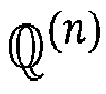

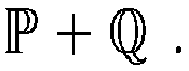


-
THEOREM 1. Letbe certain function class and

 be the distribution of g(Z). Let
 be an n-sample empirical distribution of g(Z) + ε, where Z follows distribution such that


- Letbe the distribution of ĝ(Z), then


- for the constant Cd only depending on d from
Theorem 2. - PROOF. Let,
 and
and be the distribution of g(Z) + ε, g(Z), and ĝ(Z) respectively. By triangle inequality,

- The first term on the RHS can be bounded by

- where the inequality is due to the fact that


- It is sufficient to bound these two terms to obtain the desired result.



- By
Lemma 4 and Jensen's inequality, one obtains
- Since g is an L -Lipschitz function, let
 be n-sample empirical distribution of Z. Suppose


- By
Theorem 2, we have
- By LEMMA (5),

- Combining these bounds, one obtains

as desired. -
LEMMA 4. Let, and
and be distributions on
 , then

- PROOF. Let γ be the optimal joint distribution for the infimum of


- Hence the argument can always be reduced to the case the optimal gamma exists. Hence, without loss of generality, it may be assumed that γ exists. Let γ' be the joint distribution of (X, Y) such that


as desired. -
LEMMA 5. Letand be distributions on
 . Let
. Let and
and be the empirical distribution of
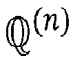 and
and , respectively. Then:

- PROOF. Use the definition


- One obtains

- Introduced is a theorem from Nicolas Fournier and Arnaud Guillin, "On the rate of convergence in Wasserstein distance of the empirical measure," Probability Theory and Related Fields 162, 3-4 (2015), 707-738, which provides the bound between empirical distribution and original distribution in Wasserstein distance.
- THEOREM 2 (
THEOREM 1 in the Fournier and Guillin document referenced above) Letbe distribution on and
and be its n-sample empirical distribution. Suppose


- for some constant Cd only depending on d.
- It shall be noted that these experiments and results are provided by way of illustration and were performed under specific conditions using a specific embodiment or embodiments; accordingly, neither these experiments nor their results shall be used to limit the scope of the disclosure of the current patent document.
- In this section, an embodiment of the likelihood estimation methodology is first evaluated with various data sets. Then, an embodiment of the methodology is applied to anomaly detection tasks. In the following experiments, "InvGAN" is used to represent an embodiment or embodiments of the present patent document. The implementation of the InvGAN embodiment or embodiments used in testing were based on the PaddlePaddle platform.
- In this subsection, an embodiment is investigated using simulated data. There are two independent and identically distributed (iid) latent variables z 1, z 2 following N(0,1) distribution. The samples are simulated with

- A tested embodiment model was compared with two density estimation models FlowGAN, and FlowVAE. FlowGAN is a hybrid model with maximum likelihood estimation (MLE) and adversarial loss. They employ coupling layers (as proposed in Laurent Dinh, Jascha Sohl-Dickstein, and Samy Bengio, "Density estimation using Real NVP," in 5th International Conference on Learning Representations (ICLR), Toulon, France (2017)) for the generator. With the coupling layers, the generator has the same number of dimensions for both latent space and input space. With the coupling layers, the determinate of the generator can be easily computed, and thus the likelihood of the samples. FlowGAN trains the generator based on both MLE and the adversarial the loss functions. A FlowVAE model was built with the decoder that had the same structure as the generator in the FlowGAN model. The InvGAN embodiment and the FlowGAN model had the sample structure for the discriminator, which includes four linear layers and three Relu layers. The same batch size and epoch number was used to train the three models.
- As state previously, the data set was simulated with 2 latent variables, and the dimension of the input (sample) space was 6. Since FlowGAN and FlowVAE use the same dimension number for both input space and the latent space, this may result in a constant offset between the model estimations and the ground truth likelihood. To fairly compare different models in figures, a constant value was added to the likelihood values of both FlowGAN and FlowVAE.
FIG. 4 gives the comparison between the ground truth and the estimated likelihood values for the testing set with three methods, according to embodiments of the present disclosure. - As shown in
FIG. 4 , the upperleft plot 400A shows the InvGAN embodiment log-likelihoods of the simulated testing set; the upperright plot 400B presents the objective loss values over iterations; the lower two plots (400C and 400D) give the log-likelihood values of the simulated data set using FlowVAE and FlowGAN. For plots with log-likelihood values, the Y-axis is the log-likelihood value, and the X-axis is sample index based on the increasing order of the ground truth log-likelihood value. It can be seen that compared with FlowGAN and FlowVAE, the tested embodiment can give more smooth estimations for the likelihood values, and improved fitting with the ground truth likelihood curve. -
FIG. 5 depicts a method for likelihood estimation, according to embodiments of the present disclosure. The depicted method uses (505) a set of input data and three trained networks-a trained generator network (g), a trained inference network (h), and trained variance network (σ). In one or more embodiments, the trained inference network (h) is used to obtain (510) a set of hidden variables (z) corresponding to the set of input data. The set of hidden variables are input (515) into the trained generator network (g) and the trained variance network (σ). A set of Riemannian metric matrices may then be computed (520) using a Jacobian matrix or matrices for the trained generator network (g) and the trained variance network (σ) regarding the set of hidden variables. Finally, log-likelihood values for the set of input data may be computed (525) using the set of Riemannian metric matrices and the log-likelihood values of the set of hidden variablesTable 1: Bits/dim on testing data sets for different models; lower is better Model Data Set 1 Data Set 2Data Set 3RealNVP 1.06 3.49 4.28 Glow 1.05 3.35 4.09 FFJORD 0.99 3.40 - MADE 2.04 5.67 - MAF 1.89 4.31 - FlowGAN 3.26 4.21 - InvGAN 1.29 1.23 1.02 - The tested embodiment was compared with the other likelihood estimation methods using three data sets. The methods listed in the Table 1 include RealNVP, Glow, FFJord, FlowGAN, MADE, and MAF (George Papamakarios, Iain Murray, and Theo Pavlakou, "Masked Autoregressive Flow for Density Estimation," in Advances in Neural Information Processing Systems (NIPS). Long Beach, CA, 2338-2347 (2017)). Most of these methods are based on maximum likelihood estimation (MLE). FlowGAN is a hybrid model combining MLE and adversarial loss. RealNVP, Glow, and FlowGAN rely on revertible coupling layers to preserve the density mass between the input space to latent space. Different from invertible neural network models, MADE and MAF are mask-based neural density estimation methods. For this set of experiments, three convolution layers and one linear layer were used for the generator, the discriminator, and the inference network. More details about the network structures are given in Appendix A.
- For the InvGAN embodiment, different number of dim() may lead to different values of log-likelihood values even for the same data sample (see the

top plot 600A inFIG. 6). FIG. 6 presents, in afirst plot 600A, the average negative log-likelihood values of Data set 1 testing data using the InvGAN embodiment at different latent space dimension (d) 600A, according to embodiments of the present disclosure. The bits-per-dimension metric, i.e., -logpx (x)/D, x ∈ RD, may not apply to the tested embodiment model, as the tested embodiment yields the smallest bits/dim value due the small latent space dimension number used in the model. To fairly compare with the other models, a revised version of bits-per-dimension metric was used in the comparison, which is
bottom plot 600B ofFIG. 6). FIG. 6 presents, in asecond plot 600B, the corresponding bits/dim for the testing set under the revised metric at different d value, according to embodiments of the present disclosure. The new metric can compensate the difference resulted from different latent space dimension numbers. For flow or reversible neural network-based density estimation methods, the value of bits-per-dim does change as they take D = d. The experimental setup in FFJord and FlowGAN was followed, and - Table 1 compares different methods under the new metric on testing data sets. The likelihood values presented in FFJord and FlowGAN were used. It can be seen that even with the revised metric, the tested embodiment model consistently performed better compared with other models.
-
FIG. 7 depicts a method for anomaly detection, according to embodiments of the present disclosure. Given a set of training data, a method like that ofFIGS. 3A-B may be used to train (705) the networks. Given a set of test data (or evaluation data, i.e., data to be evaluated), a method like that ofFIG. 5 may be used to obtain (710) log-likelihood values. In one or more embodiments, the log-likelihood values are used (715) to compute anomaly scores for the set of test data, and responsive to an anomaly score not exceeding a threshold value, the test data sample may be designated (720) as being an anomaly.Table 2: Statistics of the data sets for anomaly detection Data Set Feature Instance Data set 1 ∼1,000 60,000 Data set 2 ∼3,000 60,000 Data set 3 ∼274 ∼450 - In this subsection, a likelihood estimation embodiment is used for three anomaly detection tasks. Table 2 gives more details on the three data sets. For all of the results, the anomaly score was defined similar to Samet Akcay, Amir Atapour Abarghouei, and Toby P. Breckon, "GANomaly: Semi-supervised Anomaly Detection via Adversarial Training," in 14th Asian Conference on Computer Vision (ACCV). Perth, Australia, 622-637 (2018). With the log-likelihood value set,


- Hereis the testing set. The anomaly methods that were compared against an embodiment are given in next subsection.

- Deep Structured Energy Based Models (DSEBM) (Shuangfei Zhai, Yu Cheng, Weining Lu, and Zhongfei Zhang, "Deep Structured Energy Based Models for Anomaly Detection," in Proceedings of the 33nd International Conference on Machine Learning (ICML). New York, NY, 1100-1109 (2016)) are energy-based models for anomaly detection. Similar to denoising auto-encoder, the main idea is to accumulate the energy across layers of neural networks. Two types of anomaly scoring criteria were proposed: energy-based and reconstruction error-based. In the experimental results, DSEBM-r represents results with reconstruction error and DSEBM-e are results with energy-based approach.
- Deep Autoencoding Gaussian Mixture Model (DAGMM) (Bo Zong, Qi Song, Martin Renqiang Min, Wei Cheng, Cristian Lumezanu, Dae-ki Cho, and Haifeng Chen, "Deep Autoencoding Gaussian Mixture Model for Unsupervised Anomaly Detection," in 6th International Conference on Learning Representations (ICLR). Vancouver, BC, Canada (2018)) is an autoencoder-based method for anomaly detection, and it can achieve state-of-the-art results. In DAGMM, an auto-encoder as well as an estimator network are trained jointly. The auto-encoder is used to generate latent space representations, and the estimator is used to output parameters of a GMM modeling the lower-dimensional latent space. The likelihood value of a sample's latent representation computed with the learned GMM is taken as the anomaly detection metric.
- AnoGAN (Thomas Schlegl, Philipp Seeböck, Sebastian M. Waldstein, Ursula Schmidt-Erfurth, and Georg Langs, "Unsupervised Anomaly Detection with Generative Adversarial Networks to Guide Marker Discovery," in Proceedings of 25th International Conference on Information Processing in Medical Imaging (IPMI). Boone, NC, 146-157 (2017)) is a GAN-based method for anomaly detection. The method trains a GAN model to recover a latent representation for each test data sample. The anomaly score is calculated with a combination of the reconstruction error and the discrimination score from the discriminator network. The reconstruction error measures how well the GAN can reconstruct the data via the inferred latent variable and the generator. The authors of AnoGAN compare the two components for the anomaly score and the variant which performed best in the paper was selected.
- Efficient GAN-Based Anomaly Detection (EGBAD) (Houssam Zenati, Manon Romain, Chuan-Sheng Foo, Bruno Lecouat, and Vijay Chandrasekhar, "Adversarially Learned Anomaly Detection," in IEEE International Conference on Data Mining (ICDM). Singapore, 727-736 (2018)) is another anomaly detection method based on GAN. Different from AnoGAN, their model learns an inverse function of the generator to speed up the inference of the latent variable. Similar to AnoGAN, the anomaly score in this approach includes two parts: the fitting error from reconstruction and the discrimination score.
- GANomaly uses a conditional generative adversarial network that jointly learns the generation of high-dimensional image space and the inference of latent space. Employing encoder-decoder-encoder sub-networks in the generator enables the model to map the input image to a lower dimension vector, which is then used to reconstruct the generated output image. The use of the additional encoder network maps this generated image to its latent representation. Minimizing the distance between these images and the latent vectors during training aids in learning the effective representations for the normal samples.
- Adversarially Learned Anomaly Detection (ALAD) (Houssam Zenati, Manon Romain, Chuan-Sheng Foo, Bruno Lecouat, and Vijay Chandrasekhar, "Adversarially Learned Anomaly Detection," in IEEE International Conference on Data Mining (ICDM). Singapore, 727-736 (2018)) is a recently proposed GAN-based anomaly detection method. Similar to EGBAD (Shuangfei Zhai, Yu Cheng, Weining Lu, and Zhongfei Zhang, "Deep Structured Energy Based Models for Anomaly Detection," in Proceedings of the 33nd International Conference on Machine Learning (ICML). New York, NY, 1100-1109 (2016)), ALAD learns an encoding function to infer the latent variable for testing samples. Their model is enhanced with three discriminators. With a cycle consistence between sample space and latent space, the training of their model can be stabilized in learning representations for anomaly detection.
- One Class Support Vector Machines (OC-SVM) (Bernhard Schölkopf, Robert C. Williamson, Alexander J. Smola, John Shawe-Taylor, and John C. Platt, "Support Vector Method for Novelty Detection," in Advances in Neural Information Processing Systems (NIPS). Denver, CO, 582-588 (1999)) are a classic kernel method for anomaly detection and density estimation that learns a decision boundary around normal examples. The radial basis function (RBF) kernel is employed in the experiments. The ν parameter is set to the expected anomaly proportion in the data set, which is assumed to be known, whereas the γ parameter is set to be inversely proportional to the number of input features.
- Isolation Forests (IF) (Fei Tony Liu, Kai Ming Ting, and Zhi-Hua Zhou, "Isolation Forest," in Proceedings of the 8th IEEE International Conference on Data Mining (ICDM). Pisa, Italy, 413-422 (2008)) are a classic machine learning technique that isolates abnormal samples rather than learning the distribution of normal data. The method constructs trees across randomly chosen features according to randomly split values. The anomaly score is defined as the average path length from a testing sample to the root. The experiments results for this model were obtained with the implementation in the scikit-learn package.
- One class of the ten numbers in
Data set 1 were taken as the abnormal class, and the rest classes were taken as the normal class. In the training phase, the images from the nine normal classes were to train GAN and an embodiment of the present disclosure. In the testing state, the images from all ten classes in the testing set were used. The experiment set up followed GANomaly. The results for GANomaly were obtained by running the online code with the optimal parameters given in the script. The results for the other methods were based on the result section in GANomaly, referenced above. Theupper plot 800A inFIG. 8 shows the results of all of the methods on ten classes. Note that the order in each set of five bars inplot 800A is the same: VAE, AnoGAN, EGBAD, GANomaly, and a tested embodiment, which is labeled as InvGAN. The tested embodiment method, InvGAN, outperforms the other methods in all the ten tasks. - Similar to
Data set 1, one class was taken as the abnormal class, and the rest of the classes were taken as normal. The experimental set up as in the GANomaly document, cited above. The testing involved samples from both the normal classes and the abnormal class in the testing data set. As shown in thelower plot 800B inFIG. 8 , the tested embodiment method, InvGAN, leads the best results in all ten anomaly detection tasks, especially for the class dog. Note that the order in each set of four bars inplot 800B is the same: AnoGAN, EGBAD, GANomaly, and a tested embodiment, which is labeled as InvGAN. The anomaly detection results on two real data sets show that the tested embodiment model can perform well on the variance estimation for the distribution samples and outliers.Table 3: Anomaly detection on Data set 1 and Data set 2Data Set Model AUROC DATA SET 1 VAE 0.3420 ± 0.1861 AnoGAN 0.4390 ± 0.116 GANomaly 0.7390 ± 0.0882 InvGAN 0.7920 ± 0.0786 DATA SET 2OC-SVM* 0.5843 ± 0.0956 IF* 0.6025 ± 0.1040 DSEBM-r* 0.6071 ± 0.1007 DSEBM-e* 0.5956 ± 0.1151 ALAD* 0.6072 ± 0.1201 AnoGAN 0.5949 ± 0.1076 EGBAD 0.4450 ± 0.0786 GANomaly 0.6065 ± 0.0390 InvGAN 0.6391 ± 0.0608 - Table 3 presents comparison among different anomaly detection methods for both image data sets. The experimental setups for AnoGAN, EGBAD, GANomaly, and the proposed InvGAN were the same and follow the GANomaly document, cited above. In order to obtain a comprehensive comparison with existing methods, some anomaly detection results for Data set 2 (models marked with * in Table 3) were also included.
- It was noticed that there were some small experimental differences between ALAD and what was used here for
Data set 2. In the ALAD document, they take one class as the normal one, and the rest classes as the abnormal ones. Anomaly detection is essentially a binary classification problem. The numerical results in Table 3 can validate the significance of the tested model embodiment. In summary, the tested method embodiment outperforms the other auto-encoder and GAN based approaches for both data sets. More details about the implementation of the networks are given in Appendix A. - An embodiment was further tested on a tabular data set. The smallest classes were combined to form the anomaly class, and the rest of the classes were combined to form the normal class. Table 4 shows the anomaly detection results with different methods. Due to the small training set, classic methods outperform deep generative models on precision and F1 score. However, the tested method embodiment achieved the highest recall values and a high F1 score as well. With the help of the variance network, the tested embodiment was relatively robust compared with other deep neural network methods. More details about the implementation of the InvGAN embodiment can be found in Appendix B.
FIG. 9 gives the convergence of the loss Lh,σ for different data sets: 900A (Data set 1), 900B (Data set 2), 900C (Data set 3), and 900D (Data set 4).Table 4: Anomaly detection on Data set 4Data Set Model Precision Recall F1 Score Data set 4 OC-SVM 0.5397 0.4082 0.4581 IF 0.5147 0.5469 0.5303 DSEBM-r 0.1515 0.1513 0.1510 DSEBM-e 0.4667 0.4565 0.4601 DAGMM 0.4909 0.5078 0.4983 AnoGAN 0.4118 0.4375 0.4242 ALAD 0.5000 0.5313 0.5152 InvGAN 0.4390 0.6000 0.5070 - In this patent document, embodiments of an approach to estimate the implicit likelihoods of GANs were presented. In one or more embodiments, by leveraging an inference function and a variance network of the generator, the likelihoods of testing samples can be estimated. Simulation study and likelihood testing on data sets validate the advantages of embodiments. An embodiment was further applied to three anomaly detection tasks. Experimental results show that the tested embodiment can outperform classic and other deep neural network-based anomaly detection methods.
- The generator, discriminator, and the inference network for
Data set 1 and Data set 2 are given in Tables 5, 6, and 7. In the experiments, for Data set 3 the same network structure was used as withData set 2, and it is not stated in the tables.Table 5: Generator of InvGAN in likelihood and anomaly detection experiments for Data set 1 and Data set 2Generator Layer Number of Output Kernel Stride Activation function Input z ∼ N(0,1)50 50 Fully-Connected 128∗4∗4 ReLU Transposed convolution 128∗8∗8 4∗4 2 ReLU Transposed convolution 64∗16∗16 4∗4 2 ReLU Transposed convolution 1∗32∗32 (Data set 1) 4∗4 2 Tanh 3∗32∗32 (Data set 2) 4∗4 2 Tanh Table 6: Discriminator of the InvGAN embodiment in likelihood and anomaly detection experiments for Data set 1 and Data set 2Discriminator Layer Number of Output Kernel Stride Activation function Input x 1∗32∗32 (Data set 1) 3∗32∗32 (Data set 2) Convolution 64∗16∗16 4∗4 2 ReLU Convolution 128∗8∗8 4∗4 2 ReLU Convolution 128∗4∗4 4∗4 2 ReLU Fully-Connected 1 1 Sigmoid Table 7: Inference network of the InvGAN embodiment in likelihood and anomaly detection experiments for Data set 1 and Data set 2Inference network Layer Number of Output Kernel Stride Activation function Input x 1∗32∗32 (Data Set 1) 3∗32∗32 (Data Set 2) Convolution 64∗16∗16 4∗4 2 ReLU Convolution 128∗8∗8 4∗4 2 ReLU Convolution 128∗4∗4 4∗4 2 ReLU Fully-Connected 50 50 - The network structures for the generator, the discriminator, and the inference network in the Data set 4 experiments are given in Tables 8, 9, and 10, respectively.
Table 8: Generator of the InvGAN embodiment in Data set 4 anomaly detection experimentsGenerator Layer Number of Output Batch Normalization Activation function Input z ∼ N(0,1) z dim 50 Fully-Connected 128 Y ReLU Fully-Connected 256 Y ReLU Fully-Connected 274 Table 9: Discriminator of the InvGAN embodiment in Data set 4 anomaly detection experimentsDiscriminator Layer Number of Output Batch Normalization Activation function Input x 274 Fully-Connected 256 Y ReLU Fully-Connected 128 Y ReLU Fully-Connected 1 Sigmoid Table 10: Inference network of the InvGAN embodiment in Data set 4 anomaly detection experimentsInference Network Layer Number of Output Batch Normalization Activation function Input x 274 Fully-Connected 256 Y ReLU Fully-Connected 128 Y ReLU Fully-Connected 50 - In one or more embodiments, aspects of the present patent document may be directed to, may include, or may be implemented on one or more information handling systems/computing systems. A computing system may include any instrumentality or aggregate of instrumentalities operable to compute, calculate, determine, classify, process, transmit, receive, retrieve, originate, route, switch, store, display, communicate, manifest, detect, record, reproduce, handle, or utilize any form of information, intelligence, or data. For example, a computing system may be or may include a personal computer (e.g., laptop), tablet computer, phablet, personal digital assistant (PDA), smart phone, smart watch, smart package, server (e.g., blade server or rack server), a network storage device, camera, or any other suitable device and may vary in size, shape, performance, functionality, and price. The computing system may include random access memory (RAM), one or more processing resources such as a central processing unit (CPU) or hardware or software control logic, ROM, and/or other types of memory. Additional components of the computing system may include one or more disk drives, one or more network ports for communicating with external devices as well as various input and output (I/O) devices, such as a keyboard, a mouse, touchscreen and/or a video display. The computing system may also include one or more buses operable to transmit communications between the various hardware components.
-
FIG. 10 depicts a simplified block diagram of a computing device/information handling system (or computing system) according to embodiments of the present disclosure. It will be understood that the functionalities shown forsystem 1000 may operate to support various embodiments of a computing system-although it shall be understood that a computing system may be differently configured and include different components, including having fewer or more components as depicted inFIG. 10 . - As illustrated in
FIG. 10 , thecomputing system 1000 includes one or more central processing units (CPU) 1001 that provides computing resources and controls the computer.CPU 1001 may be implemented with a microprocessor or the like, and may also include one or more graphics processing units (GPU) 1019 and/or a floating-point coprocessor for mathematical computations.System 1000 may also include asystem memory 1002, which may be in the form of random-access memory (RAM), read-only memory (ROM), or both. - A number of controllers and peripheral devices may also be provided, as shown in
FIG. 10 . Aninput controller 1003 represents an interface to various input device(s) 1004, such as a keyboard, mouse, touchscreen, and/or stylus. Thecomputing system 1000 may also include astorage controller 1007 for interfacing with one ormore storage devices 1008 each of which includes a storage medium such as magnetic tape or disk, or an optical medium that might be used to record programs of instructions for operating systems, utilities, and applications, which may include embodiments of programs that implement various aspects of the present disclosure. Storage device(s) 1008 may also be used to store processed data or data to be processed in accordance with the disclosure. Thesystem 1000 may also include adisplay controller 1009 for providing an interface to adisplay device 1011, which may be a cathode ray tube (CRT), a thin film transistor (TFT) display, organic light-emitting diode, electroluminescent panel, plasma panel, or other type of display. Thecomputing system 1000 may also include one or more peripheral controllers orinterfaces 1005 for one ormore peripherals 1006. Examples of peripherals may include one or more printers, scanners, input devices, output devices, sensors, and the like. Acommunications controller 1014 may interface with one ormore communication devices 1015, which enables thesystem 1000 to connect to remote devices through any of a variety of networks including the Internet, a cloud resource (e.g., an Ethernet cloud, a Fiber Channel over Ethernet (FCoE)/Data Center Bridging (DCB) cloud, etc.), a local area network (LAN), a wide area network (WAN), a storage area network (SAN) or through any suitable electromagnetic carrier signals including infrared signals. - In the illustrated system, all major system components may connect to a
bus 1016, which may represent more than one physical bus. However, various system components may or may not be in physical proximity to one another. For example, input data and/or output data may be remotely transmitted from one physical location to another. In addition, programs that implement various aspects of the disclosure may be accessed from a remote location (e.g., a server) over a network. Such data and/or programs may be conveyed through any of a variety of machine-readable medium including, but are not limited to: magnetic media such as hard disks, floppy disks, and magnetic tape; optical media such as CD-ROMs and holographic devices; magneto-optical media; and hardware devices that are specially configured to store or to store and execute program code, such as application specific integrated circuits (ASICs), programmable logic devices (PLDs), flash memory devices, and ROM and RAM devices. - Aspects of the present disclosure may be encoded upon one or more non-transitory computer-readable media with instructions for one or more processors or processing units to cause steps to be performed. It shall be noted that the one or more non-transitory computer-readable media may include volatile and/or non-volatile memory. It shall be noted that alternative implementations are possible, including a hardware implementation or a software/hardware implementation. Hardware-implemented functions may be realized using ASIC(s), programmable arrays, digital signal processing circuitry, or the like. Accordingly, the "means" terms in any claims are intended to cover both software and hardware implementations. Similarly, the term "computer-readable medium or media" as used herein includes software and/or hardware having a program of instructions embodied thereon, or a combination thereof. With these implementation alternatives in mind, it is to be understood that the figures and accompanying description provide the functional information one skilled in the art would require to write program code (i.e., software) and/or to fabricate circuits (i.e., hardware) to perform the processing required.
- It shall be noted that embodiments of the present disclosure may further relate to computer products with a non-transitory, tangible computer-readable medium that have computer code thereon for performing various computer-implemented operations. The media and computer code may be those specially designed and constructed for the purposes of the present disclosure, or they may be of the kind known or available to those having skill in the relevant arts. Examples of tangible computer-readable media include, but are not limited to: magnetic media such as hard disks, floppy disks, and magnetic tape; optical media such as CD-ROMs and holographic devices; magneto-optical media; and hardware devices that are specially configured to store or to store and execute program code, such as application specific integrated circuits (ASICs), programmable logic devices (PLDs), flash memory devices, and ROM and RAM devices. Examples of computer code include machine code, such as produced by a compiler, and files containing higher level code that are executed by a computer using an interpreter. Embodiments of the present disclosure may be implemented in whole or in part as machine-executable instructions that may be in program modules that are executed by a processing device. Examples of program modules include libraries, programs, routines, objects, components, and data structures. In distributed computing environments, program modules may be physically located in settings that are local, remote, or both.
- One skilled in the art will recognize no computing system or programming language is critical to the practice of the present disclosure. One skilled in the art will also recognize that a number of the elements described above may be physically and/or functionally separated into sub-modules or combined together.
- It will be appreciated to those skilled in the art that the preceding examples and embodiments are exemplary and not limiting to the scope of the present disclosure. It is intended that all permutations, enhancements, equivalents, combinations, and improvements thereto that are apparent to those skilled in the art upon a reading of the specification and a study of the drawings are included within the true spirit and scope of the present disclosure. It shall also be noted that elements of any claims may be arranged differently including having multiple dependencies, configurations, and combinations.
Claims (23)
- A computer-implemented method for training a generative adversarial network system, the method comprising:responsive to a stop condition not being reached, repeating steps for training a generative adversarial network system comprising a generator network, a discriminator network, an inference network, and a variance network, the steps comprising:sampling a first minibatch of input data samples from an input data set;sampling a minibatch of hidden variable values from a hidden variable prior distribution;updating the discriminator network using first loss function;sampling a second minibatch of hidden variable values from the hidden variable prior distribution;updating the generator network using a second loss function;sampling a second minibatch of input data samples from the input data set;updating the inference network and the variance network using a third loss function;sampling a third minibatch of hidden variable values from the hidden variable prior distribution; andupdating the inference network and the generator network using a fourth loss function; andresponsive to a stop condition being reached, output a trained generator network, a trained inference network, and a trained variance network.
- The computer-implemented method of Claim 1 further comprising the step of:
obtaining a plurality of clusters of hidden variable values by sampling a number of hidden variable values from the hidden variable prior distribution and using K-means clustering to obtain the plurality of clusters. - The computer-implemented method of Claim 1 wherein the step of updating the inference network comprises:
training the inference network to map a given input data sample in an input space to a hidden variable value that can be mapped back to a value within a region of the input data sample in a manifold. - The computer-implemented method of Claim 1 wherein the third loss function comprises:
a difference between the generator network estimate of an input data sample using as an input the estimate of a hidden variable value obtained using the inference network and the input data sample. - The computer-implemented method of Claim 4 wherein the third loss function further comprises:
for the input data sample, determining a variance value using the variance network operating on the estimate of the hidden variable value obtained using the inference network and the input data sample. - The computer-implemented method of Claim 1 wherein the fourth loss function comprises:
a difference between a sampled hidden variable value and an estimate of the sampled hidden variable value obtained from the inference network using as an input an estimate of an input data sample for the sampled hidden variable, in which the estimate of the input data sample is obtained from the generator network and the sampled hidden variable value. - A computer-implemented method for likelihood estimation of data, the method comprising:obtain a set of latent variable values corresponding to a set of input data values using a trained inference network, which has been trained to map an input data value to a latent variable value that can be mapped back to a value within a region of the input data value in a manifold using a trained generator network;inputting the set of latent variable values into the trained generator network and a trained variance network, which has been trained to map a latent variable to a variance value that captures a local regional uncertainty in an input space;determining a set of Riemannian metric matrices using one or more Jacobian matrices for the trained generator network and the trained variance network regarding the set of latent variable values; anddetermining log-likelihood values for the set of input data values using the set of Riemannian metric matrices and log-likelihood values of the set of latent variable values.
- The computer-implemented method of Claim 7 wherein the trained generator network, the trained inference network, and the trained variance network were obtained by training a Generative Adversarial Network (GAN) system that comprised the generator network, the inference network, and the variance network.
- The computer-implemented method of Claim 7 wherein the step of training the GAN system that comprises the generator network, the inference network, and the variance network comprises the steps of:responsive to a stop condition not being reached, repeating steps for training the GAN system comprising the generator network, a discriminator network, the inference network, and the variance network, the steps comprising:sampling a first minibatch of input data samples from an input data set;sampling a minibatch of latent variable values from a latent variable prior distribution;updating the discriminator network using first loss function;sampling a second minibatch of latent variable values from the latent variable prior distribution;updating the generator network using a second loss function;sampling a second minibatch of input data samples from the input data set;updating the inference network and the variance network using a third loss function;sampling a third minibatch of latent variable values from the latent variable prior distribution; andupdating the inference network and the generator network using a fourth loss function; andresponsive to a stop condition being reached, output a trained generator network, a trained inference network, and a trained variance network.
- The computer-implemented method of Claim 9 further comprising:
obtaining a plurality of clusters of latent variable values by sampling a number of latent variable values from the latent variable prior distribution and using K-means clustering to obtain the plurality of clusters. - The computer-implemented method of Claim 9 wherein the third loss function comprises:
a difference between the generator network estimate of an input data sample using as an input the estimate of a latent variable value obtained using the inference network and the input data sample. - The computer-implemented method of Claim 11 wherein the third loss function further comprises:
for the input data sample, determining a variance value using the variance network operating on the estimate of the latent variable value obtained using the inference network and the input data sample. - The computer-implemented method of Claim 9 wherein the fourth loss function comprises:
a difference between a sampled latent variable value and an estimate of the sampled latent variable value obtained from the inference network using as an input an estimate of an input data sample for the sampled latent variable, in which the estimate of the input data sample is obtained from the generator network and the sampled latent variable value. - A computer-implemented method for anomaly detection, the method comprising:obtain a set of latent variable values corresponding to a set of input data values using a trained inference network, which has been trained to map an input data value to a latent variable value that can be mapped back to a value within a region of the input data value in a manifold using a trained generator network;inputting the set of latent variable values into the trained generator network and a trained variance network, which has been trained to map a latent variable to a variance value that captures a local regional uncertainty in an input space;determining a set of Riemannian metric matrices using one or more Jacobian matrices for the trained generator network and the trained variance network regarding the set of latent variable values; anddetermining log-likelihood values for the set of input data values using the set of Riemannian metric matrices and log-likelihood values of the set of latent variable values;using at least some of the log-likelihood values to determine corresponding anomaly scores corresponding to the set of input data values; andresponsive to an anomaly score not exceeding a threshold value, designating the input data value corresponding to the anomaly score as being an anomaly.
- The computer-implemented method of Claim 14 wherein the trained generator network, the trained inference network, and the trained variance network were obtained by training a Generative Adversarial Network (GAN) system that comprised the generator network, the inference network, and the variance network.
- The computer-implemented method of Claim 14 wherein the step of training the GAN system that comprises the generator network, the inference network, and the variance network comprises the steps of:responsive to a stop condition not being reached, repeating steps for training the GAN system comprising the generator network, a discriminator network, the inference network, and the variance network, the steps comprising:sampling a first minibatch of input data samples from an input data set;sampling a minibatch of latent variable values from a latent variable prior distribution;updating the discriminator network using first loss function;sampling a second minibatch of latent variable values from the latent variable prior distribution;updating the generator network using a second loss function;sampling a second minibatch of input data samples from the input data set;updating the inference network and the variance network using a third loss function;sampling a third minibatch of latent variable values from the latent variable prior distribution; andupdating the inference network and the generator network using a fourth loss function; andresponsive to a stop condition being reached, output a trained generator network, a trained inference network, and a trained variance network.
- The computer-implemented method of Claim 16 further comprising:
obtaining a plurality of clusters of latent variable values by sampling a number of latent variable values from the latent variable prior distribution and using K-means clustering to obtain the plurality of clusters. - The computer-implemented method of Claim 16 wherein the third loss function comprises:
a difference between the generator network estimate of an input data sample using as an input the estimate of a latent variable value obtained using the inference network and the input data sample. - The computer-implemented method of Claim 18 wherein the third loss function further comprises:
for the input data sample, determining a variance value using the variance network operating on the estimate of the latent variable value obtained using the inference network and the input data sample. - The computer-implemented method of Claim 16 wherein the fourth loss function comprises:
a difference between a sampled latent variable value and an estimate of the sampled latent variable value obtained from the inference network using as an input an estimate of an input data sample for the sampled latent variable, in which the estimate of the input data sample is obtained from the generator network and the sampled latent variable value. - A non-transitory machine-readable medium having instructions stored therein, which when executed by a processor, cause the processor to perform the method according to any of claims 1-20.
- A data processing system, comprising:a processor; anda memory coupled to the processor to store instructions, which when executed by the processor, cause the processor to perform the method according to any of claims 1-20.
- A computer program product having computer programs stored therein, which when executed by a processor, cause the processor to perform the method according to any of claims 1-20.
Applications Claiming Priority (1)
| Application Number | Priority Date | Filing Date | Title |
|---|---|---|---|
| US16/840,303 US11783198B2 (en) | 2020-04-03 | 2020-04-03 | Estimating the implicit likelihoods of generative adversarial networks |
Publications (2)
| Publication Number | Publication Date |
|---|---|
| EP3905141A1 true EP3905141A1 (en) | 2021-11-03 |
| EP3905141B1 EP3905141B1 (en) | 2026-02-04 |
Family
ID=73856086
Family Applications (1)
| Application Number | Title | Priority Date | Filing Date |
|---|---|---|---|
| EP20215923.2A Active EP3905141B1 (en) | 2020-04-03 | 2020-12-21 | Estimating the implicit likelihoods of generative adversarial networks |
Country Status (3)
| Country | Link |
|---|---|
| US (1) | US11783198B2 (en) |
| EP (1) | EP3905141B1 (en) |
| CN (1) | CN113496247B (en) |
Families Citing this family (24)
| Publication number | Priority date | Publication date | Assignee | Title |
|---|---|---|---|---|
| EP3671660B1 (en) * | 2018-12-20 | 2025-06-18 | Dassault Systèmes | Designing a 3d modeled object via user-interaction |
| EP3975055B1 (en) * | 2020-09-29 | 2025-09-24 | Robert Bosch GmbH | Estimating reliability of control data |
| US11843623B2 (en) * | 2021-03-16 | 2023-12-12 | Mitsubishi Electric Research Laboratories, Inc. | Apparatus and method for anomaly detection |
| CN116089827B (en) * | 2021-11-01 | 2026-06-05 | 中移(上海)信息通信科技有限公司 | Industrial sensor data anomaly detection methods, devices and equipment |
| CN114037853B (en) * | 2021-11-11 | 2024-03-05 | 西北工业大学 | Depth image clustering method based on Laplacian rank constraint |
| CN114399465B (en) * | 2021-12-08 | 2022-11-25 | 紫东信息科技(苏州)有限公司 | Benign and malignant ulcer identification method and system |
| CN114362859B (en) * | 2021-12-28 | 2024-03-29 | 杭州电子科技大学 | Adaptive channel modeling method and system for enhanced condition generation countermeasure network |
| CN114092472B (en) * | 2022-01-19 | 2022-05-03 | 宁波海棠信息技术有限公司 | Method, device and medium for detecting uncertain samples in defect detection |
| US12299896B1 (en) * | 2022-03-23 | 2025-05-13 | Amazon Technologies, Inc. | Synthetic image generation by manifold modification of a machine learning model |
| CN115130562B (en) * | 2022-06-13 | 2025-06-06 | 深蓝汽车科技有限公司 | A vehicle battery anomaly recognition method and system based on adversarial learning fusion clustering |
| CN117408931A (en) * | 2022-07-06 | 2024-01-16 | 纬创资通(昆山)有限公司 | Image defect detection system, production method and computer-readable recording medium |
| CN115527216B (en) * | 2022-11-09 | 2023-05-23 | 中国矿业大学(北京) | Text image generation method based on modulation fusion and antagonism network generation |
| CN115642603B (en) * | 2022-11-09 | 2026-03-20 | 永嘉县电力实业有限公司 | Large-scale power flow sample solution method based on physical knowledge neural network |
| CN116010875B (en) * | 2022-12-01 | 2026-01-23 | 国网重庆市电力公司营销服务中心 | Method and device for classifying ammeter faults, electronic equipment and computer storage medium |
| CN115905928B (en) * | 2022-12-23 | 2026-02-06 | 焦点科技股份有限公司 | Query abnormality detection method based on semi-supervised learning |
| US20240305522A1 (en) * | 2023-03-08 | 2024-09-12 | Dell Products L.P. | Method to Clone Failure Models for Real-Time Action Sequencing |
| EP4435781B8 (en) * | 2023-03-23 | 2026-04-29 | GN Hearing A/S | Audio device with uncertainty quantification and related methods |
| CN116451095B (en) * | 2023-03-27 | 2026-06-02 | 华南理工大学 | Multi-source heterogeneous medical data multi-view clustering methods, devices, media and equipment |
| CN116754230B (en) * | 2023-04-25 | 2026-05-19 | 山东省计算中心(国家超级计算济南中心) | A Bearing Anomaly Detection and Fault Diagnosis Method Based on Deep Convolutional Generative Adversarial Networks |
| CN116702010B (en) * | 2023-07-05 | 2026-02-10 | 中国电力科学研究院有限公司 | Methods, devices, equipment and media for identifying abnormal events in power distribution networks |
| CN116563673B (en) * | 2023-07-10 | 2023-12-12 | 浙江华诺康科技有限公司 | Smoke training data generation method and device and computer equipment |
| CN117133304B (en) * | 2023-07-20 | 2026-08-11 | 北京交通大学 | A method for fault detection of railway facilities |
| TWI866351B (en) * | 2023-07-25 | 2024-12-11 | 台達電子工業股份有限公司 | Generative adversarial networks-based method for component anomaly detection and device thereof |
| CN121884226A (en) * | 2025-12-29 | 2026-04-17 | 易帮客信息科技(连云港)有限公司 | Intelligent security system and method based on artificial intelligence |
Family Cites Families (37)
| Publication number | Priority date | Publication date | Assignee | Title |
|---|---|---|---|---|
| US4969097A (en) * | 1985-09-18 | 1990-11-06 | Levin Leonid D | Method of rapid entering of text into computer equipment |
| JPH07334625A (en) * | 1994-06-06 | 1995-12-22 | Nec Corp | Character string input device |
| US6321158B1 (en) * | 1994-06-24 | 2001-11-20 | Delorme Publishing Company | Integrated routing/mapping information |
| US5864340A (en) * | 1996-08-22 | 1999-01-26 | International Business Machines Corporation | Mobile client computer programmed to predict input |
| US5805159A (en) * | 1996-08-22 | 1998-09-08 | International Business Machines Corporation | Mobile client computer interdependent display data fields |
| JPH10154144A (en) * | 1996-11-25 | 1998-06-09 | Sony Corp | Text input device and method |
| JP3889466B2 (en) * | 1996-11-25 | 2007-03-07 | ソニー株式会社 | Text input device and method |
| US8479122B2 (en) * | 2004-07-30 | 2013-07-02 | Apple Inc. | Gestures for touch sensitive input devices |
| US6337698B1 (en) * | 1998-11-20 | 2002-01-08 | Microsoft Corporation | Pen-based interface for a notepad computer |
| US7881936B2 (en) * | 1998-12-04 | 2011-02-01 | Tegic Communications, Inc. | Multimodal disambiguation of speech recognition |
| US7293231B1 (en) * | 1999-03-18 | 2007-11-06 | British Columbia Ltd. | Data entry for personal computing devices |
| US7030863B2 (en) * | 2000-05-26 | 2006-04-18 | America Online, Incorporated | Virtual keyboard system with automatic correction |
| US20020024506A1 (en) * | 1999-11-09 | 2002-02-28 | Flack James F. | Motion detection and tracking system to control navigation and display of object viewers |
| US6922810B1 (en) * | 2000-03-07 | 2005-07-26 | Microsoft Corporation | Grammar-based automatic data completion and suggestion for user input |
| US20020049795A1 (en) * | 2000-05-15 | 2002-04-25 | Freeman Alfred Boyd | Computer assisted text input system |
| US20020156864A1 (en) * | 2000-06-06 | 2002-10-24 | Kniest James Newton | System for wireless exchange of data with hand held devices |
| US6704024B2 (en) * | 2000-08-07 | 2004-03-09 | Zframe, Inc. | Visual content browsing using rasterized representations |
| US7194404B1 (en) * | 2000-08-31 | 2007-03-20 | Semantic Compaction Systems | Linguistic retrieval system and method |
| WO2005008444A2 (en) * | 2003-07-14 | 2005-01-27 | Matt Pallakoff | System and method for a portbale multimedia client |
| US20050195221A1 (en) * | 2004-03-04 | 2005-09-08 | Adam Berger | System and method for facilitating the presentation of content via device displays |
| US20060020904A1 (en) * | 2004-07-09 | 2006-01-26 | Antti Aaltonen | Stripe user interface |
| US8381135B2 (en) * | 2004-07-30 | 2013-02-19 | Apple Inc. | Proximity detector in handheld device |
| US7653883B2 (en) * | 2004-07-30 | 2010-01-26 | Apple Inc. | Proximity detector in handheld device |
| US7949642B2 (en) * | 2004-10-12 | 2011-05-24 | Wendy W Yang | System and method for managing and presenting entity information |
| US20060095842A1 (en) * | 2004-11-01 | 2006-05-04 | Nokia Corporation | Word completion dictionary |
| US7886233B2 (en) * | 2005-05-23 | 2011-02-08 | Nokia Corporation | Electronic text input involving word completion functionality for predicting word candidates for partial word inputs |
| US8396582B2 (en) * | 2008-03-08 | 2013-03-12 | Tokyo Electron Limited | Method and apparatus for self-learning and self-improving a semiconductor manufacturing tool |
| US10452992B2 (en) * | 2014-06-30 | 2019-10-22 | Amazon Technologies, Inc. | Interactive interfaces for machine learning model evaluations |
| US10475174B2 (en) * | 2017-04-06 | 2019-11-12 | General Electric Company | Visual anomaly detection system |
| US10034645B1 (en) * | 2017-04-13 | 2018-07-31 | The Board Of Trustees Of The Leland Stanford Junior University | Systems and methods for detecting complex networks in MRI image data |
| CN107563355B (en) * | 2017-09-28 | 2021-04-02 | 哈尔滨工程大学 | A Generative Adversarial Network-Based Hyperspectral Anomaly Detection Method |
| US11030485B2 (en) * | 2018-03-30 | 2021-06-08 | Arizona Board Of Regents On Behalf Of Arizona State University | Systems and methods for feature transformation, correction and regeneration for robust sensing, transmission, computer vision, recognition and classification |
| US11132444B2 (en) * | 2018-04-16 | 2021-09-28 | International Business Machines Corporation | Using gradients to detect backdoors in neural networks |
| US11403750B2 (en) * | 2018-06-13 | 2022-08-02 | Siemens Healthcare Gmbh | Localization and classification of abnormalities in medical images |
| US10719301B1 (en) * | 2018-10-26 | 2020-07-21 | Amazon Technologies, Inc. | Development environment for machine learning media models |
| US11568307B2 (en) * | 2019-05-20 | 2023-01-31 | International Business Machines Corporation | Data augmentation for text-based AI applications |
| US12530775B2 (en) * | 2020-07-01 | 2026-01-20 | University Of Iowa Research Foundation | Model-based deep learning for globally optimal surface segmentation |
-
2020
- 2020-04-03 US US16/840,303 patent/US11783198B2/en active Active
- 2020-12-21 EP EP20215923.2A patent/EP3905141B1/en active Active
- 2020-12-24 CN CN202011554390.9A patent/CN113496247B/en active Active
Non-Patent Citations (20)
| Title |
|---|
| ADITYA GROVERMANIK DHARSTEFANO ERMON: "FlowGAN: Combining Maximum Likelihood and Adversarial Learning in Generative Models", PROCEEDINGS OF THE THIRTY-SECOND AAAI CONFERENCE ON ARTIFICIAL INTELLIGENCE (AAAI), 2018, pages 3069 - 3076 |
| BERNHARD SCHOLKOPFROBERT C. WILLIAMSONALEXANDER J. SMOLAJOHN SHAWE-TAYLORJOHN C. PLATT: "Support Vector Method for Novelty Detection", ADVANCES IN NEURAL INFORMATION PROCESSING SYSTEMS (NIPS), 1999, pages 582 - 588 |
| BO ZONGQI SONGMARTIN RENQIANG MINWEI CHENGCRISTIAN LUMEZANUDAE-KI CHOHAIFENG CHEN: "Deep Autoencoding Gaussian Mixture Model for Unsupervised Anomaly Detection", 6TH INTERNATIONAL CONFERENCE ON LEARNING REPRESENTATIONS (ICLR), 2018 |
| DIEDERIK P. KINGMAPRAFULLA DHARIWAL: "Glow: Generative Flow with Invertible I x I Convolutions", ADVANCES IN NEURAL INFORMATION PROCESSING SYSTEMS (NEURIPS), 2018, pages 10236 - 10245 |
| FEI TONY LIUKAI MING TINGZHI-HUA ZHOU: "Isolation Forest", PROCEEDINGS OF THE 8TH IEEE INTERNATIONAL CONFERENCE ON DATA MINING (ICDM), 2008, pages 413 - 422 |
| GAUERHOF LYDIA ET AL: "Reverse Variational Autoencoder for Visual Attribute Manipulation and Anomaly Detection", 2020 IEEE WINTER CONFERENCE ON APPLICATIONS OF COMPUTER VISION (WACV), IEEE, 1 March 2020 (2020-03-01), pages 2103 - 2112, XP033770970, DOI: 10.1109/WACV45572.2020.9093319 * |
| GEORGE PAPAMAKARIOSLAIN MURRAYTHEO PAVLAKOU: "Masked Autoregressive Flow for Density Estimation", ADVANCES IN NEURAL INFORMATION PROCESSING SYSTEMS (NIPS), 2017, pages 2338 - 2347 |
| GEORGIOS ARVANITIDIS ET AL: "Latent Space Oddity: on the Curvature of Deep Generative Models", ARXIV.ORG, CORNELL UNIVERSITY LIBRARY, 201 OLIN LIBRARY CORNELL UNIVERSITY ITHACA, NY 14853, 31 October 2017 (2017-10-31), XP081307822 * |
| HOUSSAM ZENATIMANON ROMAINCHUAN-SHENG FOOBRUNO LECOUATVIJAY CHANDRASEKHAR: "Adversarially Learned Anomaly Detection", IEEE INTERNATIONAL CONFERENCE ON DATA MINING (ICDM), 2018, pages 727 - 736, XP033485615, DOI: 10.1109/ICDM.2018.00088 |
| LAURENT DINHJASCHA SOHL-DICKSTEINSAMY BENGIO: "Density estimation using Real NVP", 5TH INTERNATIONAL CONFERENCE ON LEARNING REPRESENTATIONS (ICLR), 2017 |
| LAURENT DINHJASCHA SOHL-DICKSTEINSAMY BENGIO: "Density estimation using Real NVP", 5TH INTERNATIONAL CONFERENCE ON LEARNING REPRESENTATIONS (ICLR), TOULON, FRANCE, 2017 |
| MATHIEU GERMAINKAROL GREGORLAIN MURRAYHUGO LAROCHELLE: "MADE: Masked Autoencoder for Distribution Estimation", PROCEEDINGS OF THE 32ND INTERNATIONAL CONFERENCE ON MACHINE LEARNING (ICML), 2015, pages 881 - 889 |
| NICOLAS FOURNIERARNAUD GUILLIN: "On the rate of convergence in Wasserstein distance of the empirical measure", PROBABILITY THEORY AND RELATED FIELDS, vol. 162, no. 3-4, 2015, pages 707 - 738 |
| QICHAO QUEMIKHAIL BELKIN: "Back to the Future: Radial Basis Function Networks Revisited", PROCEEDINGS OF THE 19TH INTERNATIONAL CONFERENCE ON ARTIFICIAL INTELLIGENCE AND STATISTICS (AISTATS), 2016, pages 1375 - 1383 |
| RITHESH KUMAR ET AL: "Maximum Entropy Generators for Energy-Based Models", ARXIV.ORG, CORNELL UNIVERSITY LIBRARY, 201 OLIN LIBRARY CORNELL UNIVERSITY ITHACA, NY 14853, 24 January 2019 (2019-01-24), XP081007833 * |
| SAMET AKCAYAMIR ATAPOUR ABARGHOUEITOBY P. BRECKON: "GANomaly: Semi-supervised Anomaly Detection via Adversarial Training", 14TH ASIAN CONFERENCE ON COMPUTER VISION (ACCV), 2018, pages 622 - 637 |
| SHUANGFEI ZHAIYU CHENGWEINING LUZHONGFEI ZHANG: "Deep Structured Energy Based Models for Anomaly Detection", PROCEEDINGS OF THE 33ND INTERNATIONAL CONFERENCE ON MACHINE LEARNING (ICML), 2016, pages 1100 - 1109 |
| THOMAS SCHLEGLPHILIPP SEEBOCKSEBASTIAN M. WALDSTEINURSULA SCHMIDT-ERFURTHGEORG LANGS: "Unsupervised Anomaly Detection with Generative Adversarial Networks to Guide Marker Discovery", PROCEEDINGS OF 25TH INTERNATIONAL CONFERENCE ON INFORMATION PROCESSING IN MEDICAL IMAGING (IPMI), 2017, pages 146 - 157, XP047416148, DOI: 10.1007/978-3-319-59050-9_12 |
| WILL GRATHWOHLRICKY T. Q. CHENJESSE BETTENCOURTILYA SUTSKEVERDAVID DUVENAUD: "FFJORD: Free-Form Continuous Dynamics for Scalable Reversible Generative Models", 7TH INTERNATIONAL CONFERENCE ON LEARNING REPRESENTATIONS (ICLR), 2019 |
| ZENATI HOUSSAM ET AL: "Adversarially Learned Anomaly Detection", 2018 IEEE INTERNATIONAL CONFERENCE ON DATA MINING (ICDM), IEEE, 17 November 2018 (2018-11-17), pages 727 - 736, XP033485615, DOI: 10.1109/ICDM.2018.00088 * |
Also Published As
| Publication number | Publication date |
|---|---|
| US20210319302A1 (en) | 2021-10-14 |
| EP3905141B1 (en) | 2026-02-04 |
| CN113496247B (en) | 2024-06-25 |
| US11783198B2 (en) | 2023-10-10 |
| CN113496247A (en) | 2021-10-12 |
Similar Documents
| Publication | Publication Date | Title |
|---|---|---|
| EP3905141B1 (en) | Estimating the implicit likelihoods of generative adversarial networks | |
| Zhang et al. | Detecting overlapping communities in networks using spectral methods | |
| US11295207B2 (en) | Quantum deep learning | |
| Wager et al. | Altitude training: Strong bounds for single-layer dropout | |
| US11630989B2 (en) | Mutual information neural estimation with Eta-trick | |
| Le et al. | Estimating a network from multiple noisy realizations | |
| Wang et al. | Non-negative contrastive learning | |
| Fan et al. | On hyperparameter tuning in general clustering problemsm | |
| Kawamoto et al. | Limitations in the spectral method for graph partitioning: Detectability threshold and localization of eigenvectors | |
| Han et al. | Mini-batch spectral clustering | |
| de Miranda Cardoso et al. | Learning bipartite graphs: Heavy tails and multiple components | |
| Nallapareddy et al. | EvCenterNet: Uncertainty estimation for object detection using evidential learning | |
| Górecki et al. | Linear discriminant analysis with a generalization of the Moore–Penrose pseudoinverse | |
| Abbahaddou et al. | Graph neural network generalization with gaussian mixture model based augmentation | |
| Ren et al. | Estimate the implicit likelihoods of GANs with application to anomaly detection | |
| Zhu et al. | Elastic net constraint-based tensor model for high-order graph matching | |
| Arroyo et al. | Overlapping community detection in networks via sparse spectral decomposition | |
| Mazaheri et al. | Robust correction of sampling bias using cumulative distribution functions | |
| Jo et al. | Discrete-valued latent preference matrix estimation with graph side information | |
| Zuo et al. | Hierarchical prompts for rehearsal-free continual learning | |
| Peng et al. | Subspace clustering with active learning | |
| Park et al. | Uncertainty-based data-wise label smoothing for calibrating multiple instance learning in histopathology image classification | |
| Su et al. | On the interplay between graph structure and learning algorithms in graph neural networks | |
| Shivanna et al. | Spectral norm regularization of orthonormal representations for graph transduction | |
| Cavazos et al. | ALPCAHUS: Subspace clustering for heteroscedastic data |
Legal Events
| Date | Code | Title | Description |
|---|---|---|---|
| PUAI | Public reference made under article 153(3) epc to a published international application that has entered the european phase |
Free format text: ORIGINAL CODE: 0009012 |
|
| STAA | Information on the status of an ep patent application or granted ep patent |
Free format text: STATUS: THE APPLICATION HAS BEEN PUBLISHED |
|
| AK | Designated contracting states |
Kind code of ref document: A1 Designated state(s): AL AT BE BG CH CY CZ DE DK EE ES FI FR GB GR HR HU IE IS IT LI LT LU LV MC MK MT NL NO PL PT RO RS SE SI SK SM TR |
|
| B565 | Issuance of search results under rule 164(2) epc |
Effective date: 20211004 |
|
| STAA | Information on the status of an ep patent application or granted ep patent |
Free format text: STATUS: REQUEST FOR EXAMINATION WAS MADE |
|
| 17P | Request for examination filed |
Effective date: 20220429 |
|
| RBV | Designated contracting states (corrected) |
Designated state(s): AL AT BE BG CH CY CZ DE DK EE ES FI FR GB GR HR HU IE IS IT LI LT LU LV MC MK MT NL NO PL PT RO RS SE SI SK SM TR |
|
| STAA | Information on the status of an ep patent application or granted ep patent |
Free format text: STATUS: EXAMINATION IS IN PROGRESS |
|
| 17Q | First examination report despatched |
Effective date: 20231016 |
|
| REG | Reference to a national code |
Ref country code: DE Free format text: PREVIOUS MAIN CLASS: G06N0003040000 Ipc: G06N0003045000 Ref legal event code: R079 Ref document number: 602020066495 Country of ref document: DE |
|
| GRAP | Despatch of communication of intention to grant a patent |
Free format text: ORIGINAL CODE: EPIDOSNIGR1 |
|
| STAA | Information on the status of an ep patent application or granted ep patent |
Free format text: STATUS: GRANT OF PATENT IS INTENDED |
|
| RIC1 | Information provided on ipc code assigned before grant |
Ipc: G06N 3/045 20230101AFI20250722BHEP Ipc: G06N 3/047 20230101ALI20250722BHEP Ipc: G06N 3/084 20230101ALI20250722BHEP Ipc: G06N 3/088 20230101ALI20250722BHEP |
|
| INTG | Intention to grant announced |
Effective date: 20250806 |
|
| GRAS | Grant fee paid |
Free format text: ORIGINAL CODE: EPIDOSNIGR3 |
|
| GRAA | (expected) grant |
Free format text: ORIGINAL CODE: 0009210 |
|
| STAA | Information on the status of an ep patent application or granted ep patent |
Free format text: STATUS: THE PATENT HAS BEEN GRANTED |
|
| AK | Designated contracting states |
Kind code of ref document: B1 Designated state(s): AL AT BE BG CH CY CZ DE DK EE ES FI FR GB GR HR HU IE IS IT LI LT LU LV MC MK MT NL NO PL PT RO RS SE SI SK SM TR |
|
| REG | Reference to a national code |
Ref country code: CH Ref legal event code: F10 Free format text: ST27 STATUS EVENT CODE: U-0-0-F10-F00 (AS PROVIDED BY THE NATIONAL OFFICE) Effective date: 20260204 Ref country code: GB Ref legal event code: FG4D |
|
| REG | Reference to a national code |
Ref country code: DE Ref legal event code: R096 Ref document number: 602020066495 Country of ref document: DE |
|
| REG | Reference to a national code |
Ref country code: IE Ref legal event code: FG4D |
|
| P01 | Opt-out of the competence of the unified patent court (upc) registered |
Free format text: CASE NUMBER: UPC_APP_0002458_3905141/2026 Effective date: 20260123 |
|
| REG | Reference to a national code |
Ref country code: NL Ref legal event code: MP Effective date: 20260204 |
|
| PG25 | Lapsed in a contracting state [announced via postgrant information from national office to epo] |
Ref country code: RS Free format text: LAPSE BECAUSE OF FAILURE TO SUBMIT A TRANSLATION OF THE DESCRIPTION OR TO PAY THE FEE WITHIN THE PRESCRIBED TIME-LIMIT Effective date: 20260504 |
|
| PG25 | Lapsed in a contracting state [announced via postgrant information from national office to epo] |
Ref country code: ES Free format text: LAPSE BECAUSE OF FAILURE TO SUBMIT A TRANSLATION OF THE DESCRIPTION OR TO PAY THE FEE WITHIN THE PRESCRIBED TIME-LIMIT Effective date: 20260204 |
|
| PG25 | Lapsed in a contracting state [announced via postgrant information from national office to epo] |
Ref country code: PL Free format text: LAPSE BECAUSE OF FAILURE TO SUBMIT A TRANSLATION OF THE DESCRIPTION OR TO PAY THE FEE WITHIN THE PRESCRIBED TIME-LIMIT Effective date: 20260204 |
|
| PG25 | Lapsed in a contracting state [announced via postgrant information from national office to epo] |
Ref country code: GR Free format text: LAPSE BECAUSE OF FAILURE TO SUBMIT A TRANSLATION OF THE DESCRIPTION OR TO PAY THE FEE WITHIN THE PRESCRIBED TIME-LIMIT Effective date: 20260505 |
|
| REG | Reference to a national code |
Ref country code: LT Ref legal event code: MG9D |
|
| PG25 | Lapsed in a contracting state [announced via postgrant information from national office to epo] |
Ref country code: LT Free format text: LAPSE BECAUSE OF FAILURE TO SUBMIT A TRANSLATION OF THE DESCRIPTION OR TO PAY THE FEE WITHIN THE PRESCRIBED TIME-LIMIT Effective date: 20260204 |
|
| PG25 | Lapsed in a contracting state [announced via postgrant information from national office to epo] |
Ref country code: NO Free format text: LAPSE BECAUSE OF FAILURE TO SUBMIT A TRANSLATION OF THE DESCRIPTION OR TO PAY THE FEE WITHIN THE PRESCRIBED TIME-LIMIT Effective date: 20260504 |
|
| PG25 | Lapsed in a contracting state [announced via postgrant information from national office to epo] |
Ref country code: FI Free format text: LAPSE BECAUSE OF FAILURE TO SUBMIT A TRANSLATION OF THE DESCRIPTION OR TO PAY THE FEE WITHIN THE PRESCRIBED TIME-LIMIT Effective date: 20260204 Ref country code: AT Free format text: LAPSE BECAUSE OF FAILURE TO SUBMIT A TRANSLATION OF THE DESCRIPTION OR TO PAY THE FEE WITHIN THE PRESCRIBED TIME-LIMIT Effective date: 20260204 Ref country code: SE Free format text: LAPSE BECAUSE OF FAILURE TO SUBMIT A TRANSLATION OF THE DESCRIPTION OR TO PAY THE FEE WITHIN THE PRESCRIBED TIME-LIMIT Effective date: 20260204 |
|
| REG | Reference to a national code |
Ref country code: AT Ref legal event code: MK05 Ref document number: 1884443 Country of ref document: AT Kind code of ref document: T Effective date: 20260204 |
|
| PG25 | Lapsed in a contracting state [announced via postgrant information from national office to epo] |
Ref country code: HR Free format text: LAPSE BECAUSE OF FAILURE TO SUBMIT A TRANSLATION OF THE DESCRIPTION OR TO PAY THE FEE WITHIN THE PRESCRIBED TIME-LIMIT Effective date: 20260204 |
|
| PG25 | Lapsed in a contracting state [announced via postgrant information from national office to epo] |
Ref country code: IS Free format text: LAPSE BECAUSE OF FAILURE TO SUBMIT A TRANSLATION OF THE DESCRIPTION OR TO PAY THE FEE WITHIN THE PRESCRIBED TIME-LIMIT Effective date: 20260604 Ref country code: PT Free format text: LAPSE BECAUSE OF FAILURE TO SUBMIT A TRANSLATION OF THE DESCRIPTION OR TO PAY THE FEE WITHIN THE PRESCRIBED TIME-LIMIT Effective date: 20260605 |
|
| PG25 | Lapsed in a contracting state [announced via postgrant information from national office to epo] |
Ref country code: NL Free format text: LAPSE BECAUSE OF FAILURE TO SUBMIT A TRANSLATION OF THE DESCRIPTION OR TO PAY THE FEE WITHIN THE PRESCRIBED TIME-LIMIT Effective date: 20260204 |
|
| PG25 | Lapsed in a contracting state [announced via postgrant information from national office to epo] |
Ref country code: LV Free format text: LAPSE BECAUSE OF FAILURE TO SUBMIT A TRANSLATION OF THE DESCRIPTION OR TO PAY THE FEE WITHIN THE PRESCRIBED TIME-LIMIT Effective date: 20260204 |
|
| PG25 | Lapsed in a contracting state [announced via postgrant information from national office to epo] |
Ref country code: BG Free format text: LAPSE BECAUSE OF FAILURE TO SUBMIT A TRANSLATION OF THE DESCRIPTION OR TO PAY THE FEE WITHIN THE PRESCRIBED TIME-LIMIT Effective date: 20260204 |