EP3904172A1 - System, method and computer program for determining estimated sensor data - Google Patents
System, method and computer program for determining estimated sensor data Download PDFInfo
- Publication number
- EP3904172A1 EP3904172A1 EP20171463.1A EP20171463A EP3904172A1 EP 3904172 A1 EP3904172 A1 EP 3904172A1 EP 20171463 A EP20171463 A EP 20171463A EP 3904172 A1 EP3904172 A1 EP 3904172A1
- Authority
- EP
- European Patent Office
- Prior art keywords
- time
- sensor data
- sensor
- samples
- processing circuitry
- Prior art date
- Legal status (The legal status is an assumption and is not a legal conclusion. Google has not performed a legal analysis and makes no representation as to the accuracy of the status listed.)
- Granted
Links
Images


Classifications
-
- H—ELECTRICITY
- H04—ELECTRIC COMMUNICATION TECHNIQUE
- H04L—TRANSMISSION OF DIGITAL INFORMATION, e.g. TELEGRAPHIC COMMUNICATION
- H04L7/00—Arrangements for synchronising receiver with transmitter
- H04L7/0016—Arrangements for synchronising receiver with transmitter correction of synchronization errors
- H04L7/0033—Correction by delay
-
- H—ELECTRICITY
- H04—ELECTRIC COMMUNICATION TECHNIQUE
- H04W—WIRELESS COMMUNICATION NETWORKS
- H04W56/00—Synchronisation arrangements
- H04W56/004—Synchronisation arrangements compensating for timing error of reception due to propagation delay
- H04W56/005—Synchronisation arrangements compensating for timing error of reception due to propagation delay compensating for timing error by adjustment in the receiver
Definitions
- Examples relate to a system, method and computer program for determining estimated sensor data using time-series projection.
- Modern vehicles comprise several distributed and embedded systems.
- the climate control unit and the motor unit are separate embedded systems.
- Each of these systems may comprise one or more sensors and an Electronic Control Unit (ECU).
- the ECUs often are connected and exchange information via bus systems.
- the bus communication may require time and thus, many measurements are delayed once they arrive at an ECU.
- Embodiments of the present disclosure are based on the finding, that, in vehicles, the sensor data generated by various sensors often is out-of-sync, e.g. due to delays being introduced by the transmission of the respective sensor data over a bus system of the vehicle, or due to delays being introduced by the encoding and decoding of the sensor data for transportation of the bus.
- the delays that occur in such systems are often deterministic, i.e. they have a fixed value.
- Embodiments use time-series projection to project the trend of the sensor data into the future, to bridge the gap being introduced by the above-mentioned delays.
- Embodiments of the present disclosure may thus use time series prediction to compensate for time delays in signal transmission.
- Embodiments of the present disclosure provide a system for determining estimated sensor data of a sensor.
- the system comprises processing circuitry configured to obtain a plurality of samples of sensor data of the sensor.
- the processing circuitry is configured to obtain information on a time offset between the sensor data of the sensor and a reference time.
- the processing circuitry is configured to perform a time-series projection based on the plurality of samples of the sensor data.
- the time-series projection is performed using an auto-regressive statistical model.
- the processing circuitry is configured to determine an estimate of the sensor data for the reference time based on the time-series projection and based on the time offset between the sensor data and the reference time.
- the time-series projection may be used to bridge the time offset between the sensor data of the sensor and the reference time.
- the auto-regressive statistical model may be an auto-regressive moving average-model.
- the output value depends linearly on the current and one or more past values of a stochastic term.
- the regression error may be a linear combination of current and previous error terms.
- the auto-regressive model is applied on a differentiation of the plurality of samples of the sensor data.
- the sensor data may be made stationary, so it does not depend on the time at which the sensor data is observed.
- the auto-regressive model is applied on a once-derived version of the plurality of samples of the sensor data, which was shown to be appropriate for the types of sensor data being processed by the proposed approach.
- the auto-regressive model may be one of an Autoregressive Integrated Moving Average (ARIMA), or an Autoregressive Moving Average (ARMA) model.
- ARIMA Autoregressive Integrated Moving Average
- ARMA Autoregressive Moving Average
- ARIMA models have shown to provide a good compromise between prediction accuracy and computational effort.
- the time-series projection may be performed using at least 20 samples and/or at most 60 samples of the sensor data of the sensor.
- a lower number of samples may yield a lower computational complexity, while a larger number of samples may yield an increased accuracy.
- a number of 40 samples was found to yield a high prediction accuracy.
- the sensor data of the sensor may relate to a current of a power train of an electric vehicle.
- the sensor data of the power train may be processed in real-time to improve battery management and manage the power draw of the power train.
- the processing circuitry is configured to perform the time-series projection such, that the time offset between the sensor data and the reference time is bridged by the time-series projection.
- the processing circuitry may be configured to output the estimate of the sensor data.
- the time offset may be compensated, and another ECU may use sensor data that is estimated for the reference time.
- the processing circuitry may be configured to perform the time-series projection with a projection horizon that matches the time offset between the sensor data and the reference time.
- the time-series projection may be aimed at projecting the sensor data to the reference time.
- the sensor data may be estimated to allow a synchronization of the sensor data with sensor data of a second sensor, e.g. in order to eliminate a time offset between the two sets of sensor data.
- the reference time may be based on sensor data of a second sensor.
- the sensor data of the second sensor may comprise a second plurality of samples.
- the processing circuitry may be configured to determine the estimate of the sensor data such, that the estimate of the sensor data is time-synchronized to the latest sample of the sensor data of the second sensor. Thus, a time offset between the two sets of sensor data may be eliminated.
- the processing circuitry may be configured to obtain the sensor data of the second sensor.
- the processing circuitry may be configured to derive the time offset between the sensor data of the sensor and the reference time based on the sensor data of the second sensor and based on the sensor data of the sensor.
- the processing circuitry may determine the time offset and compensate for the determined time offset.
- the time offset may be pre-defined, or determined by another system.
- the processing circuitry is configured to output time-synchronized versions of the estimated sensor data of the sensor and of the sensor data of the second sensor. Thus, a subsequent processing of the two sets of sensor data may be facilitated.
- Embodiments of the present disclosure further provide a corresponding method for determining estimated sensor data.
- the method comprises obtaining a plurality of samples of sensor data of a sensor.
- the method comprises obtaining information on a time offset between the sensor data of the sensor and a reference time.
- the method comprises performing a time-series projection based on the plurality of samples of the sensor data.
- the time-series projection is performed using an auto-regressive statistical model.
- the method comprises determining an estimate of the sensor data for the reference time based on the time-series projection and based on the time offset between the sensor data and the reference time.
- Embodiments of the present disclosure further provide a corresponding computer program having a program code for performing the above method, when the computer program is executed on a computer, a processor, or a programmable hardware component.
- Fig. 1a shows a block diagram of an embodiment of a system 10 for determining estimated sensor data of a sensor 20.
- the system 10 comprises processing circuitry 14.
- the system further comprises an interface 12 that is coupled to the processing circuitry 14.
- the functionality of the system is provided by the processing circuitry 14, e.g. in conjunction with the interface 12.
- the processing circuitry is configured to obtain a plurality of samples of sensor data of the sensor 20.
- the processing circuitry is configured to obtain information on a time offset between the sensor data of the sensor and a reference time.
- the processing circuitry is configured to perform a time-series projection based on the plurality of samples of the sensor data.
- the time-series projection is performed using an auto-regressive statistical model.
- the processing circuitry is configured to determine an estimate of the sensor data for the reference time (i.e. with reference to the reference time, or projected to the reference time) based on the time-series projection and based on the time offset between the sensor data and the reference time.
- the system 10 may be used to process sensor data of a sensor 20 of a vehicle.
- Fig.1b shows a block diagram of an embodiment of a vehicle 100 comprising the system 10 and the sensor 20.
- the vehicle may further comprise a second sensor 30 and/or an electronic control unit 40.
- the system 10, the sensor 20 and the optional second sensor 30 and/or the optional electronic control unit 40 may communicate via a communication system (e.g. a bus system) of the vehicle, e.g. via ethernet, via a Controller Area Network Bus (CAN bus) or a Local Interconnect Network (LIN).
- a communication system e.g. a bus system
- CAN bus Controller Area Network Bus
- LIN Local Interconnect Network
- the vehicle 100 may be a land vehicle, a road vehicle, a car, an automobile, an off-road vehicle, a motor vehicle, a truck or a lorry.
- the vehicle may not be limited to roads.
- the vehicle may be a train, a ship or an airplane. While embodiments have been envisioned with vehicles in mind, embodiments may also be applied to other fields, e.g. industrial machines. Embodiments thus provide an industrial machine, such as a power plant or a manufacturing plant comprising the system 10.
- Fig. 1c shows a flow chart of a corresponding method for determining estimated sensor data.
- the method comprises obtaining 110 a plurality of samples of sensor data of a sensor.
- the method comprises obtaining 120 information on a time offset between the sensor data of the sensor and a reference time.
- the method comprises performing 130 a time-series projection based on the plurality of samples of the sensor data.
- the time-series projection is performed using an auto-regressive statistical model.
- the method comprises determining 140 an estimate of the sensor data for the reference time based on the time-series projection and based on the time offset between the sensor data and the reference time.
- Embodiments of the present disclosure relate to a system, method and computer program for determining estimated sensor data.
- the system method and computer program may be used to determine estimated sensor data in cases, in which the sensor data lags behind a reference time, e.g. due to signal processing being performed by the sensor, or due to delays being introduced by transmission of the sensor data within the system e.g. within the vehicle 100.
- the processing circuitry is configured to obtain the plurality of samples of sensor data of the sensor 20.
- the plurality of samples of the sensor data of the sensor may be samples being generated by the sensor 20.
- the plurality of samples may be equidistant in time, i.e. with a pre-defined time interval between samples.
- a timing of the plurality of samples may be based on a pre-defined sampling rate of the sensor 20, or based on pre-defined sample output rate of the sensor 20.
- the distance in time between the plurality of samples of the sensor data of the sensor (which may in the following also be denoted the first sensor) may be the same as the distance in time between a plurality of samples of sensor data of the second sensor 30 as introduced in connection with Fig. 1b ).
- the sensor data may be sensor data of a vehicular sensor, i.e. of a sensor being employed in a vehicle.
- the vehicle may be an electric vehicle (EV)
- the sensor data may be sensor data of a sensor related to the electric power train of the electric vehicle.
- the sensor data of the (first) sensor may relate to a current of a power train of an electric vehicle 100, for example to a current being output by a battery system of the electric vehicle, or to a current being used by one or more electric motors of the electric vehicle 100.
- the sensor may be a sensor of another type of distributed system, e.g. of a machine, such as an industrial plant, a robot or an airplane.
- the distributed system e.g. the vehicle, machine, industrial plant, robot, airplane etc., may comprise the system and the sensor (and optionally the second sensor).
- the processing circuitry is configured to obtain the information on the time offset between the sensor data of the sensor and the reference time.
- the information on the time offset between the sensor data of the sensor and the reference time may indicate, how far the samples of the sensor data lag behind the reference time. For example, if the current time is the reference time, a sample of the plurality of samples of the sensor data of the (first sensor) may be obtained (by the processing circuitry) at time t (e.g. the reference time), but relate to a measurement having occurred at time t - t o , with t o being the time offset.
- a similar logic may be applied if the reference time is not the current time, but for example, being defined by samples of the second sensor.
- t the reference time
- the reference time may be defined by a measurement having occurred at the second sensor, or to a time a sample of the second sensor has been received by the processing circuitry.
- the information on the time offset between the sensor data of the sensor and the reference time may define the lag or delay between the reference time and the time a sample of the sensor data of the (first) sensor is obtained by the processing circuitry, the sample being measured at a pre-defined time relative to the reference time (e.g. at the reference time).
- the information on the time offset between the sensor data of the sensor and the reference time may be received from another system (that has determined the time offset), be read-out from a memory of the system (if the time-offset is at least temporarily constant), or be determined by the processing circuitry, as will be introduced with reference to the second sensor.
- the processing circuitry is configured to perform a time-series projection (also known as time-series prediction) based on the plurality of samples of the sensor data.
- a time-series projection predicts a development of one or more numerical values over a time interval (comprising a plurality of points in time), based on historic data on the one or more numerical values.
- a trend of the one or more numerical values may be predicted based on the historic data on the numerical values, and a time-series on the development of the development of the numerical values may be predicted.
- the samples of the sensor data of the (first) sensor may be seen as time-series, with each of the samples being represented by one or more numerical values.
- the time-series projection may be applied to extend the time-series into the future (relative to the time-series), i.e. towards the reference time.
- the time-series projection may be used to projection the development of the sensor data towards the reference time, thereby closing (or at least reducing) the gap between the latest sample of the sensor data and the reference time.
- the time-series projection may be performed using an auto-regressive statistical model.
- approaches for performing a time-series projection like exponential smoothing, input the received numerical values into a pre-defined formula to obtain the estimated sensor data.
- more advanced means such as machine-learning and/or auto-regressive Markov models may be used to perform time-series projection.
- a middle ground may be used - an auto-regressive statistical model which is more complex than exponential smoothing, but less complex than the training of machine-learning models.
- exponential smoothing might not be seen as statistical models, and neither might machine-learning based approaches, such as auto-regressive Markov models.
- the auto-regressive statistical model may be a statistical model on which an estimation process for the internal parameters of the statistical model is being performed to perform the time-series projection.
- an estimation process is being shown in connection with ARMA and ARIMA models.
- the auto-regressive statistical model may be an ARMA or an ARIMA-based model.
- ARMA, and ARIMA which is an integration-based variant of ARMA, are auto-regressive statistical models that provide a time-series projection of numerical values of a time series.
- - AR stands for Auto Regressive
- MA stands for Moving Average.
- auto-regressive statistical models for time-series projection are statistical models that (only) use previous numerical values of the time-series to perform the regression-based time-series projection, i.e. the projection may be solely based on the previous numerical values of the time-series.
- the output value depends linearly on the current and one or more past values of a stochastic term.
- the regression error may be a linear combination of current and previous error terms.
- the auto-regressive statistical model may be an auto-regressive moving average-model. More details of the ARMA and ARIMA models are shown in a later part of the present disclosure.
- ARIMA models are a variant of ARMA models, where the letter "I" indicates that the model is an integrated model, i.e. a model that comprises an integration component.
- the time-series projection is being applied on differentiated version of the numerical values.
- the auto-regressive model may be applied on a differentiation of the plurality of samples of the sensor data.
- a once-derived version of the numerical values is being used.
- the auto-regressive model may be applied on a once-derived version of the plurality of samples of the sensor data.
- the differentiation may be calculated by calculating a difference between subsequent samples of the plurality of samples.
- the differentiated version (e.g. the once-derived version) of the plurality of samples may be calculated by subtracting, for each sample (bar the first) of the plurality of samples, the previous sample of the plurality of samples from the sample.
- various procedures may be applied to perform the time-series projection.
- the processes “estimation”, “validation” and “application” may be applied within the statistical model.
- estimation relates to the estimation of internal polynomial values representing the time-series.
- the processing circuitry may be configured to estimate the internal polynomial values representing the time-series, e.g. using maximum-likelihood estimation or using least-squares estimation.
- Value refers to the process of validating the time-series projection being performed based on the identified internal polynomial values, e.g.
- the processing circuitry may be configured to validate the estimated internal polynomial values representing the time-series.
- “Application” refers to the process of performing and outputting the time-series projection.
- the processing circuitry may be configured to perform the time-series projection using the estimated internal polynomial values representing the time-series.
- a process "identification” may be applied, to identify the general parameters of the ARMA or ARIMA model.
- the general parameters of the ARMA or ARIMA model may be pre-defined.
- the processing circuitry may be configured to obtain the general parameters of the ARMA or ARIMA model from memory of the system, or to determine the general parameters (e.g. using a bounded exhaustive grid search).
- the Akaike Information Criterion AIC may be used to determine the general parameters of the ARMA or ARIMA model.
- both ARMA and ARIMA models have at least two general parameters, which are generally specified as p , which is the trend autoregression order, and q, which is the trend moving average order.
- ARIMA-based models have the general parameters d , which defines the trend difference order.
- 40 previous samples were found to provide a suitable set of historic data.
- the time-series projection may be performed using at least 20 samples (or at least 30 samples) and/or at most 60 samples (or at most 50 samples) of the sensor data of the sensor, e.g. 40 samples.
- Some auto-regressive statistical models use so-called seasonality to model seasonal variations in the time-series. This is useful in time-series with seasonal changes, such as changes between weekends and weekdays, or between daytime and night-time hours. In embodiments, however, such seasonal changes might not be applicable, e.g. as the time horizon being incorporated may be too small to exhibit seasonality. Accordingly, general parameters related to seasonality may be ignored or set to zero.
- the projection horizon being used may be defined such, that it bridges the gap defined by the time-offset.
- the processing circuitry may be configured to perform the time-series projection with a projection horizon that matches the time offset between the sensor data and the reference time.
- the time-series projection may extend the sensor data of the sensor such, that the gap between the sensor data and the reference time is bridged.
- the processing circuitry may be configured to perform the time-series projection such, that the time offset between the sensor data and the reference time is bridged by the time-series projection.
- the processing circuitry is configured to determine the estimate of the sensor data for the reference time based on the time-series projection and based on the time offset between the sensor data and the reference time.
- the time-series projection may extend the sensor data of the sensor such, that the gap between the sensor data and the reference time is bridged.
- the processing circuitry may be configured to use an output of the time-series projection that corresponds to an estimate of the sensor data for the reference time to determine the estimate of the sensor data for the reference time.
- the processing circuitry may be configured to determine a single estimate of the sensor data for (i.e. at, with reference to) the reference time (relative to the current sensor data), and omit the time between the latest sample and the sample estimated for the reference time.
- the processing circuitry may be configured to output the estimate of the sensor data.
- the distributed system may comprise a second sensor.
- this second sensor may be sensor that provides sensor data with less of a gap to the reference time, or zero gap to the reference time, and may thus be used as a reference.
- the reference time may be based on sensor data of a second sensor 30.
- the reference time may be defined by the latest sample of sensor data of the second sensor, or the reference time may be in a pre-defined relationship with the sensor data of the sensor.
- the time-series projection may be used to synchronize the sensor data of the first and sensor data.
- the sensor data of the second sensor may comprise a second plurality of samples
- the processing circuitry may be configured to determine the estimate of the sensor data such, that the estimate of the sensor data is time-synchronized to the latest sample of the sensor data of the second sensor.
- the estimate of the sensor data may be determined for a point in time that matches the point in time of the latest sample of the second plurality of samples of the second sensor.
- the latest sample of the second plurality of samples may either define the reference time, or be in a pre-defined temporal relationship with the reference time.
- the distributed system e.g. the vehicle, may comprise another electronic control unit (ECU) 40, which is coupled to the system 10 (which may also be an electronic control unit).
- ECU electronice control unit
- Embodiments of the present disclosure may be used to compensate for the delay being introduced by transmissions from one electronic control unit to another, with the transmissions being performed over a bus system of the distributed system/vehicle.
- the reference time may be based on a communication delay between the system 10 and the electronic control unit 40.
- the time offset may correspond to the communication delay (or to the negative of the communication delay) between the system 10 and the electronic control unit 40.
- the processing circuitry is further configured to obtain the sensor data of the second sensor, e.g. via the interface 12.
- the sensor data of the second sensor may be used for at least one of two things - to determine the reference time, and to provide time-synchronized versions of the sensor data of the first and second sensor.
- the processing circuitry may be configured to derive the time offset between the sensor data of the sensor and the reference time based on the sensor data of the second sensor and based on the sensor data of the sensor (as the latest sample of the sensor data of the second sensor can be in a pre-defined temporal relationship with, or define, the reference time.
- the first and second sensor data may be correlated.
- the output of the battery is generally correlated with the current draw of the electric motor(s), and/or with the temperature of one or more components of the power train (as the current is not only used to generate mechanical power, but also corresponding heat in the various components).
- a change in the sensor data of the first sensor may see a corresponding (i.e.
- the processing circuitry may be configured to calculate the correlation between the sensor signal of the first sensor and several time-shifted versions of the sensor data of the second sensor (or vice versa). The time-shifted version that yields the highest degree of correlation may be based on the (correct) time offset. Thus, the processing circuitry may be configured to use a correlation analysis on time-shifted versions of the sensor data of the first and second sensor to determine the time-offset.
- the sensor data of the first and second sensor may be output in a time-synchronized manner.
- the processing circuitry may be configured to output time-synchronized versions of the estimated sensor data of the sensor and of the sensor data of the second sensor.
- the interface 12 may correspond to one or more inputs and/or outputs for receiving and/or transmitting information, which may be in digital (bit) values according to a specified code, within a module, between modules or between modules of different entities.
- the interface 12 may comprise interface circuitry configured to receive and/or transmit information.
- the processing circuitry 14 may be implemented using one or more processing units, one or more processing devices, any means for processing, such as a processor, a computer or a programmable hardware component being operable with accordingly adapted software.
- a processor any means for processing
- the described function of the processing circuitry 14 may as well be implemented in software, which is then executed on one or more programmable hardware components.
- Such hardware components may comprise a general-purpose processor, a Digital Signal Processor (DSP), a micro-controller, etc.
- DSP Digital Signal Processor
- system and method may comprise one or more additional optional features corresponding to one or more aspects of the proposed concept or one or more examples described above or below.
- Embodiments of the present disclosure relate to the enhancement of measurement quality in electronic vehicles.
- Vehicles can be likened to distributed systems, which comprise many control units (ECUs) that are connected and communicate with each other via bus systems.
- ECUs control units
- time delays may occur in bus communication. These lead to delays and thus to a loss of efficiency.
- the delays may be individual for each ECU (as the origin of the signal) and can be determined. After determining the delays, the values between the last received signal and the current time step may still be known.
- autoregressive Markov models (ARMMs) and neural networks may be used to predict the values between the last received signal and the current time step.
- Signal 1 arrives 3 time-steps later than signal 2.
- the time delay may be determined to find out that signal 1 is delayed by 3 time-steps relative to signal 2, and the signal may be corrected accordingly.
- Embodiments of the present disclosure focus on the prediction of the values of signal 1 for the current time step and the two previous time-steps.
- the current measurement signal of the high-voltage storage (HVS) is received by the control unit (ECU) delayed by about 6 time-steps compared to the signal of the electric machine in reality. Accordingly, while the signal can be corrected, and the signal values can be associated with their "actual" time, embodiments may be used to predict the 6 values that have not been received. With the help of the above-mentioned algorithms, these 6 values may be approximated/estimated from the e.g. 20 last received measured values. For example, embodiments may be used in vehicles and machines, airplanes etc.
- Various embodiments of the present disclosure relate to time series prediction for measurements of electric powertrains.
- Real-time systems require up-to-date information.
- Measurement signals in the power train of Electric Vehicles (EVs) are however often received with individual time delays due to the distributed architecture of the power train.
- Embodiments of the present disclosure provide an approach that attempts to compensate the time delays by predicting each signal from the last received value until the present time step.
- 5 time-series prediction algorithms and 2 naive methods are evaluated for time series prediction. The algorithms were applied on real power train data of EVs and the results were evaluated. The evaluation focuses on run-time, precision and accuracy. As will be shown in the following, the evaluated methods achieve a prediction error rate of less than 5 %.
- Modern vehicles comprise several distributed and embedded systems.
- the climate control unit and the motor unit are separate embedded systems.
- Each of these systems comprises one or more sensors and an Electronic Control Unit (ECU).
- the ECUs are connected and exchange information via bus systems.
- the bus communication requires time and thus, many measurements are delayed once they arrive at an ECU (see Fig. 2a ). Conversely, this means that from an ECU's perspective, measurements of the actual time step from other ECUs are not yet available (see Fig. 2b ).
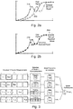
- Figs. 2a and 2b show graphs related to the availability of sensor data.
- a graph is shown, where a difference between a "real" signal 210 (labeled with crosses) and a delayed, received signal 220 (dashed line, labeled with dashed circles) is shown. Due to time delays between the distributed system in the power train of EVs, an ECU receives a delayed version 220 of the original measurement signal 210.
- Fig. 2b a scenario is shown where the delayed signal is corrected 230 (such that the received samples are attributed their correct time), so it becomes evident that the latest samples 240 are missing.
- Embodiments of the present disclosure may attempt to predict the missing values until the present (by performing a time-series projection).
- the missing or delayed availability of measurements is problematic, because many vehicular real-time control functions depend on these data and their timeliness. Especially Electric Vehicles (EVs) lose efficiency and performance due to time delays (see J. Pfeiffer and X. Wu (2019), "Automated Time Delay Estimation for Distributed Sensor Systems of Electric Vehicles ").
- Embodiments of the present disclosure may construct plausible virtual measurement values for not yet received signals. The already received measurements from past time-steps may be used to predict the values until the present.
- Exponential Smoothing is a family of time series prediction algorithms first proposed more than 60 years ago (see R. G. Brown and A. D. Little (1956), “EXPONENTIAL SMOOTHING FOR PREDICTING DEMAND ").
- the simple and the fully additive Holt-Winters model R. J. Hyndman and Y. Khandakar (2008): “Automatic Time Series Forecasting: The forecast Package for R ” is being used.
- Exponential Smoothing The basic idea of Exponential Smoothing is to construct predictions of future values ⁇ t +1 as weighted averages of past observations y t and former predictions ⁇ t . The heavier weight is thereby assigned to the more recent values. Values from the more distant past are weighted less.
- ⁇ , ⁇ and ⁇ are the corresponding smoothing coefficients. These are fitted by an optimization algorithm and have values between 0 and 1.
- ARIMA is a class of statistical models for analyzing and predicting time series data ( V. Kotu and B. Deshpande (2019), Data Science: Concepts and Practice. Cambridge, MA, United States: Elsevier, 2019 ). It is a generalization of the simpler ARMA extended by integration.
- the acronym ARIMA is descriptive and captures the key aspects of the model itself. These can be outlined in the 3 following components:
- the predicted value ⁇ t +1 of the future step t + 1 is therefore a constant and a weighted sum of one or more recent values of y or of one or more recent values of the prediction error e.
- the ARIMA model obtained in this case is a dampedtrend linear Exponential Smoothing. It extrapolates the local trend at the end of the time series. Simultaneously, it flattens the trend out at longer forecast horizons to introduce a note of conservatism.
- the dth difference ⁇ ' t +1 of the future value y t +1 is calculated. The difference is a linear combination of past values of the original time series and past values of the prediction errors.
- y ⁇ ⁇ t + 1 l t + ⁇ 0 y ⁇ ⁇ t + ⁇ 1 y ⁇ ⁇ t ⁇ 1 + ⁇ + ⁇ p y ⁇ ⁇ t ⁇ p + e t + 1 + ⁇ 0 e t + ⁇ + ⁇ q e t ⁇ q
- l t is the local level and e t the prediction error at time step t.
- ⁇ j is the slope coefficient relative to the dth difference ⁇ ' t -1 of y t-j with j ⁇ ⁇ 0,1, 2, ..., p ⁇ .
- ⁇ k is the moving average parameter relative to the prediction error e t-k with k ⁇ ⁇ 0,1, 2, ..., q ⁇ . e t +1 is hereby assumed as white noise.
- the integrated part of ARIMA is reflected in the dth difference ⁇ ' t-j of ⁇ t-j .
- a third group of algorithms relate to Box-cox transformation, ARMA residuals, Trend and Seasonality (BATS) and Trigonometric seasonal, Box-cox transformation, ARMA residuals, Trend and Seasonality (TBATS), which are an extension of the state space modeling framework shown in A. M. De Livera, R. J. Hyndman, and R. D. Snyder (2011): “Forecasting Time Series With Complex Seasonal Patterns Using Exponential Smoothing ". They introduce a comprehensive approach for predicting complex seasonal time series such as those with multiple seasonal periods, high frequency seasonality and non-integer seasonality. This is achieved by leveraging the benefits of Box-Cox transformations, Fourier representations with time varying coefficients, and ARMA error correction.
- the Box-Cox transformation solves the issues of non-linearity in the data.
- the ARMA model addresses the de-correlation of residuals in the time series data.
- De Livera et al. prove that BATS model can improve the prediction performance compared to simple state space models.
- a key feature of both frameworks is that they rely on an optimized method that greatly reduces the computational complexity of the maximum likelihood estimation.
- the BATS model is rooted in Exponential Smoothing.
- y t ⁇ is the observation at time step t Box-Cox transformed with the parameter ⁇ .
- s t i denotes the i -th seasonal component, l t the local level and b t the dampened trend.
- the notation d t stands for the ARMA ( p, q ) process for residuals.
- e t is modeled as a Gaussian white noise process.
- e t -1 stands for the i -th Box-Cox transformed prediction error.
- the Box-Cox trans-formation parameter co, the smoothing parameters ⁇ and ⁇ , the trend damping factor ⁇ , the ARMA coefficients ⁇ i and ⁇ i , as well as the seasonal smoothing factor ⁇ i can all be estimated by the means of a Gaussian likelihood process.
- TBATS extends the BATS model by including a trigonometric formulation for decomposing complex seasonal time series and identifying latent seasonal components.
- s j , t i denotes the stochastic level of the i -th seasonal component.
- s j , t ⁇ t reflects the change in the seasonal component over time.
- the number of harmonics required for the i -th seasonal component is denoted by k i .
- the trigonometric expression of seasonality terms helps to reduce the number of model parameters when the frequencies of seasonality are high. It also adds to the flexibility of the model in dealing with complex seasonality.
- Point forecasts and forecast intervals for both the TBATS and the BATS models can be obtained using the inverse BoxCox transformation of appropriate quantiles of the distribution of y n + h
- h ⁇ . h is hereby the forecasting horizon and n the number of points in the observed data y ( y 1 ,..., y n ).
- a fourth group of algorithms are in the following denoted as "Naive Methods”.
- the naive methods predict the next values of time series without further computational intelligence.
- the lack of computations or advanced models makes them very fast and demonstrates, whether the predictions of the advanced methods are really accurate, or if the same results can be achieved with less effort.
- the second naive method is a driftless Naive Random Walk.
- a time series is said to follow a Random Walk if the differences from one observation to the next one are random. In other words, the series itself is not necessarily random but its first differences are.
- Bootstrap Aggregation is a method for reducing variance without increasing the bias of predictions. It enables to achieve more accurate predictions by combining forecasts of different predictors. Combining predictions is especially useful when the uncertainty about the environment and the prediction method is relatively high, and when errors need to be moderated.
- predictors are trained on bootstrapped versions of the original data. The predictors form an ensemble. Predictions are generated by applying all predictors on the data set at hand and then combining the results. This can be achieved by averaging the obtained results, for example. Bagging tackles the three sources of uncertainties. It helps to moderate data uncertainty and the variation of the inherent random component that exist in time series.
- the reference data consists of an extensive set of recordings of current measurements in power trains of EVs.
- the measurement data are recorded on public roads and reflect the behavior of power trains of EVs under common driving conditions.
- the data set covers in total 4 h of driving data measured at a frequency of 100 Hz.
- the focus was on the 5 HV currents of the HV battery, the electric machine, the electric heating, the air-conditioning compressor and the DC/DC converter.
- the data set at hand was divided into training and test segments to apply nested cross-validation. To this end, the data was split into chunks of constant size. Each chunk consists of 20 data points. In total, 10,480 chunks are taken into consideration.
- Fig. 3 shows a chronological representation of the nested cross-validation pipeline.
- the historical HV current measurements which are split into five chunks are shown on the left.
- a first run one chunk was used as training data and one chunk was used as test data.
- two chunks were used as training data and one chunk as test data
- a third run three chunks were used as training data and one chunk as test data
- in a fourth run four chunks were used as training data and one chunk as test data.
- Training was used to select the model's hyperparameters (with one chunk of data in the first run, two chunks in the second run etc.), and the test data was used to evaluate the model.
- Each run yields an error Error 1 to Error 4
- the model performance was determined by summing Error 1 to Error 4 .
- Root Mean Square Error RMSE
- Mean Absolute Percentage Error MAE
- Analyzing the run-time performance of each prediction algorithm is important for investigating its suitability for real-time systems. If the prediction takes too much time, it may become obsolete. Therefore, all algorithms were executed several times on the same execution platform under the same circumstances and measure their run-time. In the subsequent measurement, a computer with a 2.4 GHz CPU and 8 GB of RAM was used.
- the test setup was used on identify, among a pool of 7 candidate algorithms, or their best combination. Its essence was to link the knowledge on prediction errors of different algorithms to historical data. Therefore, in the following, the focus is on the experiments applied for mapping historical current measurements to prediction method performances. In a first step, the focus is on retrieving the optimal hyper parameters of each algorithm and assessing the individual performances. In the second step, the added value of combining forecasts from different methods in reducing uncertainty and increasing forecasting accuracy is assessed.
- the individual performance of the algorithms in predicting future HV current is assessed.
- the analysis is performed under specific constraints.
- the main constraint is that the inference and prediction of future current values are based only on historical measurements.
- the performance of each algorithm is assessed using the nested cross-validation procedure described before.
- an exhaustive grid search through a manually specified subset of the hyper parameter space on the training splits was performed. This helps to identify the best combination of hyper parameters for each algorithm.
- the Akaike Information Criterion was employed as a selection metric.
- the AIC rewards the goodness of fit as assessed by the likelihood function given the number of estimated parameters k per algorithm. Simultaneously, k and the algorithm's complexity are penalized by the AIC to prevent over-fitting.
- Fig. 4b extends the results described in Fig. 4a to cover computational aspects.
- computational complexity and run-time requirements may be deemed critical to the objective of predicting HV current measurements.
- the methods of seasonal ARIMA, BATS and TBATS may be deemed obsolete. Their respective run-time may exceed our limit of at maximum 200 ms.
- the obtained forecasts may be irrelevant by the time they are computed.
- Fig. 4b shows a comparison per algorithm with regard to accuracy and efficiency.
- the bootstrap aggregation outperformed all individual methods in terms of the MAPE except for ARIMA. Accordingly, bootstrap aggregation fails to improve the overall prediction. Nevertheless, the results may be improved with an adaptive weights approach. Instead of the equal weights approach used in the context of the present disclosure, the adaptive weights approach might be able to benefit from the high accuracy of ARIMA.
- Bootstrap Aggregation has the worst runtime of all considered approaches. As the concept combines the predictions of several algorithms, it also sums up the required run-time of all these algorithms. Especially in the application field outlined above, the execution on ECUs, the long runtime may be considered a disadvantage. Regrettably, this disadvantage might not be equalized by the achieved results.
- ARIMA offers the best compromise between high accuracy and small outliers.
- the naive method is the fastest method.
- its accuracy is not far below the other methods. Its relatively good results show the difficulty of predicting HV measurements of electric power trains accurately.
- Another possibility is to combine the predictions of several algorithms with Bootstrap Aggregation.
- the here implemented equal weights approach outper-forms almost all algorithms, it is not able to achieve the low MAPE value of ARIMA. Further work is necessary to investigate, if an adaptive weights approach is able to outperform ARIMA. Until now, Bootstrap Aggregation requires by far the most run-time.
- Examples may further be or relate to a computer program having a program code for performing one or more of the above methods, when the computer program is executed on a computer or processor. Steps, operations or processes of various above-described methods may be performed by programmed computers or processors. Examples may also cover program storage devices such as digital data storage media, which are machine, processor or computer readable and encode machine-executable, processor-executable or computer-executable programs of instructions. The instructions perform or cause performing some or all of the acts of the above-described methods.
- the program storage devices may comprise or be, for instance, digital memories, magnetic storage media such as magnetic disks and magnetic tapes, hard drives, or optically readable digital data storage media.
- FIG. 1 may also cover computers, processors or control units programmed to perform the acts of the above-described methods or (field) programmable logic arrays ((F)PLAs) or (field) programmable gate arrays ((F)PGAs), programmed to perform the acts of the above-described methods.
- a functional block denoted as "means for " performing a certain function may refer to a circuit that is configured to perform a certain function.
- a "means for s.th.” may be implemented as a "means configured to or suited for s.th.”, such as a device or a circuit configured to or suited for the respective task.
- Functions of various elements shown in the figures may be implemented in the form of dedicated hardware, such as “a signal provider”, “a signal processing unit”, “a processor”, “a controller”, etc. as well as hardware capable of executing software in association with appropriate software.
- a processor the functions may be provided by a single dedicated processor, by a single shared processor, or by a plurality of individual processors, some of which or all of which may be shared.
- processor or “controller” is by far not limited to hardware exclusively capable of executing software, but may include digital signal processor (DSP) hardware, network processor, application specific integrated circuit (ASIC), field programmable gate array (FPGA), read only memory (ROM) for storing software, random access memory (RAM), and nonvolatile storage.
- DSP digital signal processor
- ASIC application specific integrated circuit
- FPGA field programmable gate array
- ROM read only memory
- RAM random access memory
- nonvolatile storage Other hardware, conventional and/or custom, may also be included.
- a block diagram may, for instance, illustrate a high-level circuit diagram implementing the principles of the disclosure.
- a flow chart, a flow diagram, a state transition diagram, a pseudo code, and the like may represent various processes, operations or steps, which may, for instance, be substantially represented in computer readable medium and so executed by a computer or processor, whether or not such computer or processor is explicitly shown.
- Methods disclosed in the specification or in the claims may be implemented by a device having means for performing each of the respective acts of these methods.
- each claim may stand on its own as a separate example. While each claim may stand on its own as a separate example, it is to be noted that - although a dependent claim may refer in the claims to a specific combination with one or more other claims - other examples may also include a combination of the dependent claim with the subject matter of each other dependent or independent claim. Such combinations are explicitly proposed herein unless it is stated that a specific combination is not intended. Furthermore, it is intended to include also features of a claim to any other independent claim even if this claim is not directly made dependent to the independent claim.
Landscapes
- Engineering & Computer Science (AREA)
- Computer Networks & Wireless Communication (AREA)
- Signal Processing (AREA)
- Electric Propulsion And Braking For Vehicles (AREA)
- Testing Or Calibration Of Command Recording Devices (AREA)
- Traffic Control Systems (AREA)
Abstract
Description
- Examples relate to a system, method and computer program for determining estimated sensor data using time-series projection.
- Modern vehicles comprise several distributed and embedded systems. For example, the climate control unit and the motor unit are separate embedded systems. Each of these systems may comprise one or more sensors and an Electronic Control Unit (ECU). The ECUs often are connected and exchange information via bus systems. The bus communication may require time and thus, many measurements are delayed once they arrive at an ECU.
- There may be a desire for an improved concept for dealing with locally-delayed sensor measurements.
- This desire is addressed by the subject-matter of the independent claims.
- Embodiments of the present disclosure are based on the finding, that, in vehicles, the sensor data generated by various sensors often is out-of-sync, e.g. due to delays being introduced by the transmission of the respective sensor data over a bus system of the vehicle, or due to delays being introduced by the encoding and decoding of the sensor data for transportation of the bus. The delays that occur in such systems are often deterministic, i.e. they have a fixed value. Embodiments use time-series projection to project the trend of the sensor data into the future, to bridge the gap being introduced by the above-mentioned delays. Embodiments of the present disclosure may thus use time series prediction to compensate for time delays in signal transmission.
- Embodiments of the present disclosure provide a system for determining estimated sensor data of a sensor. The system comprises processing circuitry configured to obtain a plurality of samples of sensor data of the sensor. The processing circuitry is configured to obtain information on a time offset between the sensor data of the sensor and a reference time. The processing circuitry is configured to perform a time-series projection based on the plurality of samples of the sensor data. The time-series projection is performed using an auto-regressive statistical model. The processing circuitry is configured to determine an estimate of the sensor data for the reference time based on the time-series projection and based on the time offset between the sensor data and the reference time. Thus, the time-series projection may be used to bridge the time offset between the sensor data of the sensor and the reference time.
- There are various types of auto-regressive statistical models. One subset of auto-regressive statistical models is based on the concept of "moving-average". In other words, the auto-regressive statistical model may be an auto-regressive moving average-model. In a moving average model, the output value depends linearly on the current and one or more past values of a stochastic term. In particular, the regression error may be a linear combination of current and previous error terms.
- In some embodiments, the auto-regressive model is applied on a differentiation of the plurality of samples of the sensor data. Using the differentiation, the sensor data may be made stationary, so it does not depend on the time at which the sensor data is observed. For example, the auto-regressive model is applied on a once-derived version of the plurality of samples of the sensor data, which was shown to be appropriate for the types of sensor data being processed by the proposed approach.
- For example, the auto-regressive model may be one of an Autoregressive Integrated Moving Average (ARIMA), or an Autoregressive Moving Average (ARMA) model. In particular ARIMA models have shown to provide a good compromise between prediction accuracy and computational effort.
- For example, the time-series projection may be performed using at least 20 samples and/or at most 60 samples of the sensor data of the sensor. A lower number of samples may yield a lower computational complexity, while a larger number of samples may yield an increased accuracy. In an evaluation of the proposed approach, a number of 40 samples was found to yield a high prediction accuracy.
- For example, the sensor data of the sensor may relate to a current of a power train of an electric vehicle. In electric vehicles (EVs), the sensor data of the power train may be processed in real-time to improve battery management and manage the power draw of the power train.
- In various embodiments, the processing circuitry is configured to perform the time-series projection such, that the time offset between the sensor data and the reference time is bridged by the time-series projection. The processing circuitry may be configured to output the estimate of the sensor data. Thus, the time offset may be compensated, and another ECU may use sensor data that is estimated for the reference time.
- For example, the processing circuitry may be configured to perform the time-series projection with a projection horizon that matches the time offset between the sensor data and the reference time. In other words, the time-series projection may be aimed at projecting the sensor data to the reference time.
- In general, the sensor data may be estimated to allow a synchronization of the sensor data with sensor data of a second sensor, e.g. in order to eliminate a time offset between the two sets of sensor data. For example, the reference time may be based on sensor data of a second sensor. The sensor data of the second sensor may comprise a second plurality of samples. The processing circuitry may be configured to determine the estimate of the sensor data such, that the estimate of the sensor data is time-synchronized to the latest sample of the sensor data of the second sensor. Thus, a time offset between the two sets of sensor data may be eliminated.
- For example, the processing circuitry may be configured to obtain the sensor data of the second sensor. The processing circuitry may be configured to derive the time offset between the sensor data of the sensor and the reference time based on the sensor data of the second sensor and based on the sensor data of the sensor. In other words, the processing circuitry may determine the time offset and compensate for the determined time offset. Alternatively, the time offset may be pre-defined, or determined by another system.
- In various embodiments, the processing circuitry is configured to output time-synchronized versions of the estimated sensor data of the sensor and of the sensor data of the second sensor. Thus, a subsequent processing of the two sets of sensor data may be facilitated.
- Embodiments of the present disclosure further provide a corresponding method for determining estimated sensor data. The method comprises obtaining a plurality of samples of sensor data of a sensor. The method comprises obtaining information on a time offset between the sensor data of the sensor and a reference time. The method comprises performing a time-series projection based on the plurality of samples of the sensor data. The time-series projection is performed using an auto-regressive statistical model. The method comprises determining an estimate of the sensor data for the reference time based on the time-series projection and based on the time offset between the sensor data and the reference time.
- Embodiments of the present disclosure further provide a corresponding computer program having a program code for performing the above method, when the computer program is executed on a computer, a processor, or a programmable hardware component.
- Some examples of apparatuses and/or methods will be described in the following by way of example only, and with reference to the accompanying figures, in which
- Fig. 1a
- shows a block diagram of an embodiment of a system for determining estimated sensor data;
- Fig.1b
- shows a block diagram of an embodiment of a vehicle comprising a system for determining estimated sensor data;
- Fig. 1c
- shows a flow chart of a method for determining estimated sensor data;
- Figs. 2a and 2b
- show graphs related to the availability of sensor data;
- Fig. 3
- shows a chronological representation of a nested cross-validation pipeline; and
- Figs. 4a and 4b
- show tables of overviews of prediction and runtime performance scores obtained by algorithms being evaluated.
- Various examples will now be described more fully with reference to the accompanying drawings in which some examples are illustrated. In the figures, the thicknesses of lines, layers and/or regions may be exaggerated for clarity.
- Accordingly, while further examples are capable of various modifications and alternative forms, some particular examples thereof are shown in the figures and will subsequently be described in detail. However, this detailed description does not limit further examples to the particular forms described. Further examples may cover all modifications, equivalents, and alternatives falling within the scope of the disclosure. Same or like numbers refer to like or similar elements throughout the description of the figures, which may be implemented identically or in modified form when compared to one another while providing for the same or a similar functionality.
- It will be understood that when an element is referred to as being "connected" or "coupled" to another element, the elements may be directly connected or coupled via one or more intervening elements. If two elements A and B are combined using an "or", this is to be understood to disclose all possible combinations, i.e. only A, only B as well as A and B, if not explicitly or implicitly defined otherwise. An alternative wording for the same combinations is "at least one of A and B" or "A and/or B". The same applies, mutatis mutandis, for combinations of more than two Elements.
- The terminology used herein for the purpose of describing particular examples is not intended to be limiting for further examples. Whenever a singular form such as "a," "an" and "the" is used and using only a single element is neither explicitly or implicitly defined as being mandatory, further examples may also use plural elements to implement the same functionality. Likewise, when a functionality is subsequently described as being implemented using multiple elements, further examples may implement the same functionality using a single element or processing entity. It will be further understood that the terms "comprises," "comprising," "includes" and/or "including," when used, specify the presence of the stated features, integers, steps, operations, processes, acts, elements and/or components, but do not preclude the presence or addition of one or more other features, integers, steps, operations, processes, acts, elements, components and/or any group thereof.
- Unless otherwise defined, all terms (including technical and scientific terms) are used herein in their ordinary meaning of the art to which the examples belong.
-
Fig. 1a shows a block diagram of an embodiment of asystem 10 for determining estimated sensor data of asensor 20. Thesystem 10 comprises processingcircuitry 14. Optionally, the system further comprises aninterface 12 that is coupled to theprocessing circuitry 14. In general, the functionality of the system is provided by theprocessing circuitry 14, e.g. in conjunction with theinterface 12. For example, the processing circuitry is configured to obtain a plurality of samples of sensor data of thesensor 20. The processing circuitry is configured to obtain information on a time offset between the sensor data of the sensor and a reference time. The processing circuitry is configured to perform a time-series projection based on the plurality of samples of the sensor data. The time-series projection is performed using an auto-regressive statistical model. The processing circuitry is configured to determine an estimate of the sensor data for the reference time (i.e. with reference to the reference time, or projected to the reference time) based on the time-series projection and based on the time offset between the sensor data and the reference time. - For example, the
system 10 may be used to process sensor data of asensor 20 of a vehicle. Accordingly,Fig.1b shows a block diagram of an embodiment of avehicle 100 comprising thesystem 10 and thesensor 20. Optionally, the vehicle may further comprise asecond sensor 30 and/or anelectronic control unit 40. Thesystem 10, thesensor 20 and the optionalsecond sensor 30 and/or the optionalelectronic control unit 40 may communicate via a communication system (e.g. a bus system) of the vehicle, e.g. via ethernet, via a Controller Area Network Bus (CAN bus) or a Local Interconnect Network (LIN). For example, thevehicle 100 may be a land vehicle, a road vehicle, a car, an automobile, an off-road vehicle, a motor vehicle, a truck or a lorry. In general, the vehicle may not be limited to roads. For example, the vehicle may be a train, a ship or an airplane. While embodiments have been envisioned with vehicles in mind, embodiments may also be applied to other fields, e.g. industrial machines. Embodiments thus provide an industrial machine, such as a power plant or a manufacturing plant comprising thesystem 10. -
Fig. 1c shows a flow chart of a corresponding method for determining estimated sensor data. The method comprises obtaining 110 a plurality of samples of sensor data of a sensor. The method comprises obtaining 120 information on a time offset between the sensor data of the sensor and a reference time. The method comprises performing 130 a time-series projection based on the plurality of samples of the sensor data. The time-series projection is performed using an auto-regressive statistical model. The method comprises determining 140 an estimate of the sensor data for the reference time based on the time-series projection and based on the time offset between the sensor data and the reference time. - The following description relates both to the system of
Figs. 1a and/or 1b and to the method ofFig. 1c . Features described in connection with the system ofFigs. 1a and/or 1b may likewise be applied to the method ofFig. 1c . - Embodiments of the present disclosure relate to a system, method and computer program for determining estimated sensor data. As has been laid out before, the system method and computer program may be used to determine estimated sensor data in cases, in which the sensor data lags behind a reference time, e.g. due to signal processing being performed by the sensor, or due to delays being introduced by transmission of the sensor data within the system e.g. within the
vehicle 100. - The processing circuitry is configured to obtain the plurality of samples of sensor data of the
sensor 20. In general, the plurality of samples of the sensor data of the sensor may be samples being generated by thesensor 20. The plurality of samples may be equidistant in time, i.e. with a pre-defined time interval between samples. For example, a timing of the plurality of samples may be based on a pre-defined sampling rate of thesensor 20, or based on pre-defined sample output rate of thesensor 20. In various embodiments, the distance in time between the plurality of samples of the sensor data of the sensor (which may in the following also be denoted the first sensor) may be the same as the distance in time between a plurality of samples of sensor data of thesecond sensor 30 as introduced in connection withFig. 1b ). - There are a variety of types of sensor data the proposed approach can be applied on. For example, the sensor data may be sensor data of a vehicular sensor, i.e. of a sensor being employed in a vehicle. For example, the vehicle may be an electric vehicle (EV), and the sensor data may be sensor data of a sensor related to the electric power train of the electric vehicle. For example, the sensor data of the (first) sensor may relate to a current of a power train of an
electric vehicle 100, for example to a current being output by a battery system of the electric vehicle, or to a current being used by one or more electric motors of theelectric vehicle 100. Alternatively, the sensor may be a sensor of another type of distributed system, e.g. of a machine, such as an industrial plant, a robot or an airplane. In general, the distributed system, e.g. the vehicle, machine, industrial plant, robot, airplane etc., may comprise the system and the sensor (and optionally the second sensor). - The processing circuitry is configured to obtain the information on the time offset between the sensor data of the sensor and the reference time. In general, the information on the time offset between the sensor data of the sensor and the reference time may indicate, how far the samples of the sensor data lag behind the reference time. For example, if the current time is the reference time, a sample of the plurality of samples of the sensor data of the (first sensor) may be obtained (by the processing circuitry) at time t (e.g. the reference time), but relate to a measurement having occurred at time t - to , with to being the time offset. A similar logic may be applied if the reference time is not the current time, but for example, being defined by samples of the second sensor. In this case, t, the reference time, may be defined by a measurement having occurred at the second sensor, or to a time a sample of the second sensor has been received by the processing circuitry. In any case, the information on the time offset between the sensor data of the sensor and the reference time may define the lag or delay between the reference time and the time a sample of the sensor data of the (first) sensor is obtained by the processing circuitry, the sample being measured at a pre-defined time relative to the reference time (e.g. at the reference time). In general, the information on the time offset between the sensor data of the sensor and the reference time may be received from another system (that has determined the time offset), be read-out from a memory of the system (if the time-offset is at least temporarily constant), or be determined by the processing circuitry, as will be introduced with reference to the second sensor.
- The processing circuitry is configured to perform a time-series projection (also known as time-series prediction) based on the plurality of samples of the sensor data. In general, a time-series projection predicts a development of one or more numerical values over a time interval (comprising a plurality of points in time), based on historic data on the one or more numerical values. In other words, a trend of the one or more numerical values may be predicted based on the historic data on the numerical values, and a time-series on the development of the development of the numerical values may be predicted. In embodiments, the samples of the sensor data of the (first) sensor may be seen as time-series, with each of the samples being represented by one or more numerical values. The time-series projection may be applied to extend the time-series into the future (relative to the time-series), i.e. towards the reference time. In other words, the time-series projection may be used to projection the development of the sensor data towards the reference time, thereby closing (or at least reducing) the gap between the latest sample of the sensor data and the reference time.
- The time-series projection may be performed using an auto-regressive statistical model. In general, there are a variety of approaches for performing a time-series projection. Some approaches, like exponential smoothing, input the received numerical values into a pre-defined formula to obtain the estimated sensor data. Alternatively, more advanced means, such as machine-learning and/or auto-regressive Markov models may be used to perform time-series projection. In embodiments, a middle ground may be used - an auto-regressive statistical model which is more complex than exponential smoothing, but less complex than the training of machine-learning models. In other words, exponential smoothing might not be seen as statistical models, and neither might machine-learning based approaches, such as auto-regressive Markov models. In embodiments, the auto-regressive statistical model may be a statistical model on which an estimation process for the internal parameters of the statistical model is being performed to perform the time-series projection. In the following, such an internal estimation process is being shown in connection with ARMA and ARIMA models.
- As has been laid out before, the auto-regressive statistical model may be an ARMA or an ARIMA-based model. ARMA, and ARIMA, which is an integration-based variant of ARMA, are auto-regressive statistical models that provide a time-series projection of numerical values of a time series. To take apart the acronyms - AR stands for Auto Regressive and MA stands for Moving Average. In general, auto-regressive statistical models for time-series projection are statistical models that (only) use previous numerical values of the time-series to perform the regression-based time-series projection, i.e. the projection may be solely based on the previous numerical values of the time-series. In a moving average model, the output value depends linearly on the current and one or more past values of a stochastic term. In particular, the regression error may be a linear combination of current and previous error terms. Accordingly, the auto-regressive statistical model may be an auto-regressive moving average-model. More details of the ARMA and ARIMA models are shown in a later part of the present disclosure.
- As has been pointed out above, ARIMA models are a variant of ARMA models, where the letter "I" indicates that the model is an integrated model, i.e. a model that comprises an integration component. More particular, in ARIMA, the time-series projection is being applied on differentiated version of the numerical values. In other words, the auto-regressive model may be applied on a differentiation of the plurality of samples of the sensor data. In ARIMA, oftentimes, a once-derived version of the numerical values is being used. In other words, the auto-regressive model may be applied on a once-derived version of the plurality of samples of the sensor data. In general, the differentiation may be calculated by calculating a difference between subsequent samples of the plurality of samples. In other words, the differentiated version (e.g. the once-derived version) of the plurality of samples may be calculated by subtracting, for each sample (bar the first) of the plurality of samples, the previous sample of the plurality of samples from the sample.
- In general, in ARMA or ARIMA-based models, various procedures may be applied to perform the time-series projection. In general, the processes "estimation", "validation" and "application" may be applied within the statistical model. In general, "estimation" relates to the estimation of internal polynomial values representing the time-series. In other words, the processing circuitry may be configured to estimate the internal polynomial values representing the time-series, e.g. using maximum-likelihood estimation or using least-squares estimation. "Validation" refers to the process of validating the time-series projection being performed based on the identified internal polynomial values, e.g. in terms of whether error residuals being generated by the time-series values are uncorrelated and/or whether the error residuals behave like white noise. In other words, the processing circuitry may be configured to validate the estimated internal polynomial values representing the time-series. "Application" refers to the process of performing and outputting the time-series projection. In other words, the processing circuitry may be configured to perform the time-series projection using the estimated internal polynomial values representing the time-series.
- In some embodiments, a process "identification" may be applied, to identify the general parameters of the ARMA or ARIMA model. Alternatively, the general parameters of the ARMA or ARIMA model may be pre-defined. In other words, the processing circuitry may be configured to obtain the general parameters of the ARMA or ARIMA model from memory of the system, or to determine the general parameters (e.g. using a bounded exhaustive grid search). For example, as will be introduced in a later part of the disclosure, the Akaike Information Criterion (AIC) may be used to determine the general parameters of the ARMA or ARIMA model.
- In general, both ARMA and ARIMA models have at least two general parameters, which are generally specified as p, which is the trend autoregression order, and q, which is the trend moving average order. In addition, ARIMA-based models have the general parameters d, which defines the trend difference order. In experiments, the parameter values p = 1, d = 1 and q = 4 were found to be suitable parameters. In other words, the ARMA model may be used with parameters p = 1 and q = 4, and the ARIMA model may be used with p = 1, d = 1 and q = 4. In addition, 40 previous samples were found to provide a suitable set of historic data. In other words, the time-series projection may be performed using at least 20 samples (or at least 30 samples) and/or at most 60 samples (or at most 50 samples) of the sensor data of the sensor, e.g. 40 samples.
- Some auto-regressive statistical models use so-called seasonality to model seasonal variations in the time-series. This is useful in time-series with seasonal changes, such as changes between weekends and weekdays, or between daytime and night-time hours. In embodiments, however, such seasonal changes might not be applicable, e.g. as the time horizon being incorporated may be too small to exhibit seasonality. Accordingly, general parameters related to seasonality may be ignored or set to zero. For example, in ARIMA, general parameters related to the seasonality of the time-series projection may be defined, such as P (Seasonal auto-regressive order), D (Seasonal difference order), Q (Seasonal moving average order) and m (The number of time steps for a single seasonal period). These general parameters may be ignored or set to zero, i.e. (P,D,Q, m) = (0, 0, 0, 0).
- In general, whatever auto-regressive statistical model is used, the projection horizon being used may be defined such, that it bridges the gap defined by the time-offset. In other words, the processing circuitry may be configured to perform the time-series projection with a projection horizon that matches the time offset between the sensor data and the reference time. For example, the time-series projection may extend the sensor data of the sensor such, that the gap between the sensor data and the reference time is bridged. In other words, the processing circuitry may be configured to perform the time-series projection such, that the time offset between the sensor data and the reference time is bridged by the time-series projection.
- The processing circuitry is configured to determine the estimate of the sensor data for the reference time based on the time-series projection and based on the time offset between the sensor data and the reference time. For example, as has been laid out before, the time-series projection may extend the sensor data of the sensor such, that the gap between the sensor data and the reference time is bridged. The processing circuitry may be configured to use an output of the time-series projection that corresponds to an estimate of the sensor data for the reference time to determine the estimate of the sensor data for the reference time. In various embodiments, at any given point in time, the processing circuitry may be configured to determine a single estimate of the sensor data for (i.e. at, with reference to) the reference time (relative to the current sensor data), and omit the time between the latest sample and the sample estimated for the reference time. Finally, the processing circuitry may be configured to output the estimate of the sensor data.
- As has been pointed out before, the distributed system, e.g. the vehicle, may comprise a second sensor. In some embodiments, this second sensor may be sensor that provides sensor data with less of a gap to the reference time, or zero gap to the reference time, and may thus be used as a reference. Accordingly, the reference time may be based on sensor data of a
second sensor 30. For example, the reference time may be defined by the latest sample of sensor data of the second sensor, or the reference time may be in a pre-defined relationship with the sensor data of the sensor. The time-series projection may be used to synchronize the sensor data of the first and sensor data. In more formal terms, the sensor data of the second sensor may comprise a second plurality of samples, and the processing circuitry may be configured to determine the estimate of the sensor data such, that the estimate of the sensor data is time-synchronized to the latest sample of the sensor data of the second sensor. In other words, the estimate of the sensor data may be determined for a point in time that matches the point in time of the latest sample of the second plurality of samples of the second sensor. Again, the latest sample of the second plurality of samples may either define the reference time, or be in a pre-defined temporal relationship with the reference time. - Alternatively or additionally, the distributed system, e.g. the vehicle, may comprise another electronic control unit (ECU) 40, which is coupled to the system 10 (which may also be an electronic control unit). Embodiments of the present disclosure may be used to compensate for the delay being introduced by transmissions from one electronic control unit to another, with the transmissions being performed over a bus system of the distributed system/vehicle. Accordingly, the reference time may be based on a communication delay between the
system 10 and theelectronic control unit 40. For example, the time offset may correspond to the communication delay (or to the negative of the communication delay) between thesystem 10 and theelectronic control unit 40. - In various embodiments, the processing circuitry is further configured to obtain the sensor data of the second sensor, e.g. via the
interface 12. The sensor data of the second sensor may be used for at least one of two things - to determine the reference time, and to provide time-synchronized versions of the sensor data of the first and second sensor. - For example, the processing circuitry may be configured to derive the time offset between the sensor data of the sensor and the reference time based on the sensor data of the second sensor and based on the sensor data of the sensor (as the latest sample of the sensor data of the second sensor can be in a pre-defined temporal relationship with, or define, the reference time. In general, the first and second sensor data may be correlated. As an example, in a power train of an electric vehicle, the output of the battery is generally correlated with the current draw of the electric motor(s), and/or with the temperature of one or more components of the power train (as the current is not only used to generate mechanical power, but also corresponding heat in the various components). Thus, a change in the sensor data of the first sensor may see a corresponding (i.e. correlated) change in the sensor data of the second sensor, the change being perceptible with the same time-offset that is being used in the time-series projection. The processing circuitry may be configured to calculate the correlation between the sensor signal of the first sensor and several time-shifted versions of the sensor data of the second sensor (or vice versa). The time-shifted version that yields the highest degree of correlation may be based on the (correct) time offset. Thus, the processing circuitry may be configured to use a correlation analysis on time-shifted versions of the sensor data of the first and second sensor to determine the time-offset.
- Additionally or alternatively, the sensor data of the first and second sensor may be output in a time-synchronized manner. In other words, the processing circuitry may be configured to output time-synchronized versions of the estimated sensor data of the sensor and of the sensor data of the second sensor.
- The
interface 12 may correspond to one or more inputs and/or outputs for receiving and/or transmitting information, which may be in digital (bit) values according to a specified code, within a module, between modules or between modules of different entities. For example, theinterface 12 may comprise interface circuitry configured to receive and/or transmit information. - In embodiments the
processing circuitry 14 may be implemented using one or more processing units, one or more processing devices, any means for processing, such as a processor, a computer or a programmable hardware component being operable with accordingly adapted software. In other words, the described function of theprocessing circuitry 14 may as well be implemented in software, which is then executed on one or more programmable hardware components. Such hardware components may comprise a general-purpose processor, a Digital Signal Processor (DSP), a micro-controller, etc. - More details and aspects of the system and method are mentioned in connection with the proposed concept or one or more examples described above or below (e.g.
Fig. 2a to 4b ). The system and method may comprise one or more additional optional features corresponding to one or more aspects of the proposed concept or one or more examples described above or below. - Embodiments of the present disclosure relate to the enhancement of measurement quality in electronic vehicles. Vehicles can be likened to distributed systems, which comprise many control units (ECUs) that are connected and communicate with each other via bus systems. Unfortunately, time delays may occur in bus communication. These lead to delays and thus to a loss of efficiency. The delays may be individual for each ECU (as the origin of the signal) and can be determined. After determining the delays, the values between the last received signal and the current time step may still be known. In some other systems, autoregressive Markov models (ARMMs) and neural networks may be used to predict the values between the last received signal and the current time step.
- To give an example:
Signal 1 arrives 3 time-steps later thansignal 2. In embodiments, the time delay may be determined to find out thatsignal 1 is delayed by 3 time-steps relative to signal 2, and the signal may be corrected accordingly. Embodiments of the present disclosure focus on the prediction of the values ofsignal 1 for the current time step and the two previous time-steps. - In the following, an evaluation of different time-series projection algorithms is shown. Five advanced and two naive different algorithms to generate the missing signal values using time series prediction from the already received values were evaluated. The algorithms considered are Exponential Smoothing (in two different versions), ARIMA, Box-cox transformation, ARMA (Autoregressive Moving Average) residuals, Trend and Seasonality (BATS) and Trigonometric seasonal, Box-cox transformation, ARMA residuals, Trend and Seasonality (TBATS) as well as the naive methods "predicted value=last received value" and Random Walk. Additionally, the combination of different algorithms via bagging or bootstrap aggregation were evaluated.
- The current measurement signal of the high-voltage storage (HVS) is received by the control unit (ECU) delayed by about 6 time-steps compared to the signal of the electric machine in reality. Accordingly, while the signal can be corrected, and the signal values can be associated with their "actual" time, embodiments may be used to predict the 6 values that have not been received. With the help of the above-mentioned algorithms, these 6 values may be approximated/estimated from the e.g. 20 last received measured values. For example, embodiments may be used in vehicles and machines, airplanes etc.
- Various embodiments of the present disclosure relate to time series prediction for measurements of electric powertrains. Real-time systems require up-to-date information. Measurement signals in the power train of Electric Vehicles (EVs) are however often received with individual time delays due to the distributed architecture of the power train. Embodiments of the present disclosure provide an approach that attempts to compensate the time delays by predicting each signal from the last received value until the present time step. In the following, 5 time-series prediction algorithms and 2 naive methods are evaluated for time series prediction. The algorithms were applied on real power train data of EVs and the results were evaluated. The evaluation focuses on run-time, precision and accuracy. As will be shown in the following, the evaluated methods achieve a prediction error rate of less than 5 %. As expected, the benchmark naive method is the fastest. Surprisingly, it retrieves comparable results to Exponential Smoothing. Box-cox transformation, ARMA (Autoregressive Moving Average) residuals, Trend and Seasonality (BATS) and Trigonometric seasonal, Box-cox transformation, ARMA residuals, Trend and Seasonality (TBATS) are the slowest algorithms. Nevertheless, they achieve the best accuracy, but suffer from outliers. ARIMA (Autoregressive Integrated Moving Average) has the highest precision and thus the best compromise between outliers and accuracy of all algorithms. Additionally, to further improve the accuracy, the benefits of combining predictions of different algorithms were evaluated.
- Modern vehicles comprise several distributed and embedded systems. For example, the climate control unit and the motor unit are separate embedded systems. Each of these systems comprises one or more sensors and an Electronic Control Unit (ECU). The ECUs are connected and exchange information via bus systems. The bus communication requires time and thus, many measurements are delayed once they arrive at an ECU (see
Fig. 2a ). Conversely, this means that from an ECU's perspective, measurements of the actual time step from other ECUs are not yet available (seeFig. 2b ). -
Figs. 2a and 2b show graphs related to the availability of sensor data. InFig. 2a , a graph is shown, where a difference between a "real" signal 210 (labeled with crosses) and a delayed, received signal 220 (dashed line, labeled with dashed circles) is shown. Due to time delays between the distributed system in the power train of EVs, an ECU receives a delayedversion 220 of theoriginal measurement signal 210. InFig. 2b , a scenario is shown where the delayed signal is corrected 230 (such that the received samples are attributed their correct time), so it becomes evident that thelatest samples 240 are missing. In other words, if the delayed signal is corrected by performing automatic time-delay estimation, it becomes evident that the measurements of the last time-steps 240 have not yet been received. Nevertheless, those actual measurements may be required for controlling the EV. Embodiments of the present disclosure may attempt to predict the missing values until the present (by performing a time-series projection). The missing or delayed availability of measurements is problematic, because many vehicular real-time control functions depend on these data and their timeliness. Especially Electric Vehicles (EVs) lose efficiency and performance due to time delays (see J. Pfeiffer and X. Wu (2019), "Automated Time Delay Estimation for Distributed Sensor Systems of Electric Vehicles"). Embodiments of the present disclosure may construct plausible virtual measurement values for not yet received signals. The already received measurements from past time-steps may be used to predict the values until the present. - In the following, four groups of algorithms are presented.
- A first group of algorithms relate to Exponential Smoothing: Exponential Smoothing is a family of time series prediction algorithms first proposed more than 60 years ago (see R. G. Brown and A. D. Little (1956), "EXPONENTIAL SMOOTHING FOR PREDICTING DEMAND"). In the following, the simple and the fully additive Holt-Winters model (R. J. Hyndman and Y. Khandakar (2008): "Automatic Time Series Forecasting: The forecast Package for R") is being used.
- The basic idea of Exponential Smoothing is to construct predictions of future values ŷ t+1 as weighted averages of past observations yt and former predictions ŷt. The heavier weight is thereby assigned to the more recent values. Values from the more distant past are weighted less. Formally, the simple Exponential Smoothing prediction equation can be written as

- An extension of this basic model is the fully additive Holt-Winters model. It predicts the value for the next time step by considering additive trend and seasonality. The seasonality aspects are included by extending the prediction from equation (1) by the 3 hidden state variables


- A second group of algorithms relate to ARIMA. ARIMA is a class of statistical models for analyzing and predicting time series data (V. Kotu and B. Deshpande (2019), Data Science: Concepts and Practice. Cambridge, MA, United States: Elsevier, 2019). It is a generalization of the simpler ARMA extended by integration. The acronym ARIMA is descriptive and captures the key aspects of the model itself. These can be outlined in the 3 following components:
- 1) Auto-Regressive (AR): A model that uses the dependent relationship between an observation and a number of lagged observations.
- 2) Integrated (I): Differentiation of raw observations to make the time series stationary. This can be achieved by subtracting an observation at the actual time step from an observation at the previous time step.
- 3) Moving Average (MA): A model making use of the dependency between an observation and residual errors from a moving average model applied to lagged observations.
- The predicted value ŷ t+1 of the future step t + 1 is therefore a constant and a weighted sum of one or more recent values of y or of one or more recent values of the prediction error e. In an example, let p = 1, d = 1, q = 2. The ARIMA model obtained in this case is a dampedtrend linear Exponential Smoothing. It extrapolates the local trend at the end of the time series. Simultaneously, it flattens the trend out at longer forecast horizons to introduce a note of conservatism. For the prediction, first, the dth difference ŷ' t+1 of the future value y t+1 is calculated. The difference is a linear combination of past values of the original time series and past values of the prediction errors. It can be computed according to



- A third group of algorithms relate to Box-cox transformation, ARMA residuals, Trend and Seasonality (BATS) and Trigonometric seasonal, Box-cox transformation, ARMA residuals, Trend and Seasonality (TBATS), which are an extension of the state space modeling framework shown in A. M. De Livera, R. J. Hyndman, and R. D. Snyder (2011): "Forecasting Time Series With Complex Seasonal Patterns Using Exponential Smoothing". They introduce a comprehensive approach for predicting complex seasonal time series such as those with multiple seasonal periods, high frequency seasonality and non-integer seasonality. This is achieved by leveraging the benefits of Box-Cox transformations, Fourier representations with time varying coefficients, and ARMA error correction. The Box-Cox transformation solves the issues of non-linearity in the data. The ARMA model addresses the de-correlation of residuals in the time series data. De Livera et al. prove that BATS model can improve the prediction performance compared to simple state space models. A key feature of both frameworks is that they rely on an optimized method that greatly reduces the computational complexity of the maximum likelihood estimation.
The BATS model is rooted in Exponential Smoothing. It reformulates equation (3) as


- Here,


- TBATS extends the BATS model by including a trigonometric formulation for decomposing complex seasonal time series and identifying latent seasonal components. The seasonal component is modeled based on a Fourier series as follows:

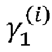


- Point forecasts and forecast intervals for both the TBATS and the BATS models can be obtained using the inverse BoxCox transformation of appropriate quantiles of the distribution of

- A fourth group of algorithms are in the following denoted as "Naive Methods". To benchmark the advanced prediction algorithms presented above and to show their effectiveness, two naive methods are introduced. The naive methods predict the next values of time series without further computational intelligence. The lack of computations or advanced models makes them very fast and demonstrates, whether the predictions of the advanced methods are really accurate, or if the same results can be achieved with less effort. The first naive method simply predicts the last measurement as future value

- The second naive method is a driftless Naive Random Walk. A time series is said to follow a Random Walk if the differences from one observation to the next one are random. In other words, the series itself is not necessarily random but its first differences are. A Random Walk for a time series is written as

- In the following, the concept of Bootstrap Aggregation is introduced. Bootstrap Aggregation, commonly known as Bagging, is a method for reducing variance without increasing the bias of predictions. It enables to achieve more accurate predictions by combining forecasts of different predictors. Combining predictions is especially useful when the uncertainty about the environment and the prediction method is relatively high, and when errors need to be moderated. In Bagging, predictors are trained on bootstrapped versions of the original data. The predictors form an ensemble. Predictions are generated by applying all predictors on the data set at hand and then combining the results. This can be achieved by averaging the obtained results, for example. Bagging tackles the three sources of uncertainties. It helps to moderate data uncertainty and the variation of the inherent random component that exist in time series. It also helps to temper the uncertainty linked with the selection of the optimal model form. Parameter uncertainty can furthermore be softened especially in terms of selecting the best set of parameters for de-scribing the data. Bergmeir et al. show an example of successfully applying bagging for time series prediction (C. Bergmeir, R. J. Hyndman, and J. M. Benitez (2016): "Bagging exponential smoothing methods using STL decomposition and Box-Cox transformation,").
- In the following, the experimental setup and the means for evaluating the results are introduced. The reference data consists of an extensive set of recordings of current measurements in power trains of EVs. The measurement data are recorded on public roads and reflect the behavior of power trains of EVs under common driving conditions. The data set covers in total 4 h of driving data measured at a frequency of 100 Hz. For the experiments, the focus was on the 5 HV currents of the HV battery, the electric machine, the electric heating, the air-conditioning compressor and the DC/DC converter. The data set at hand was divided into training and test segments to apply nested cross-validation. To this end, the data was split into chunks of constant size. Each chunk consists of 20 data points. In total, 10,480 chunks are taken into consideration.
- To better estimate the prediction error of each algorithm, a common approach is to average the errors over all the train/test splits. The technique that was used is based on a method called forward-chaining. It is referred to in the literature as rolling-origin evaluation (L. J. Tashman (2000): "Out-of-sample tests of forecasting accuracy: an analysis and review") or rolling-origin-recalibration evaluation (C. Bergmeir and J. Bentez (2012): "On the use of cross-validation for time series predictor evaluation,"). Based on this method, each data chunk was considered as the test set (see
Fig. 3 ). The previous data was assigned to the training set. Assuming that the data set can be divided in 5 chunks as shown inFig. 3 , four different training and test splits were determined. The pipeline is used to split the data set into, in this exemplary case, five training and test chunks. -
Fig. 3 shows a chronological representation of the nested cross-validation pipeline. The historical HV current measurements, which are split into five chunks are shown on the left. In a first run, one chunk was used as training data and one chunk was used as test data. In a second run, two chunks were used as training data and one chunk as test data, in a third run, three chunks were used as training data and one chunk as test data, and in a fourth run, four chunks were used as training data and one chunk as test data. Training was used to select the model's hyperparameters (with one chunk of data in the first run, two chunks in the second run etc.), and the test data was used to evaluate the model. Each run yields an error Error1 to Error4, and the model performance was determined by summing Error1 to Error4. - By producing multiple different train/test splits, a better assessment of the prediction accuracy of each algorithm was achieved. The error on each split is again averaged in order to compute a robust estimate of each algorithm's error. The overall prediction error ε is mod-eled according to


- To measure the performance of each algorithm in respect of its accuracy and computational efficiency, the following metrics are introduced: Root Mean Square Error (RMSE) and Mean Absolute Percentage Error (MAPE).
- The Root Mean Square Error (RMSE) is a quadratic scoring rule that measures the average magnitude of the error. It is the square root of the average of squared differences between prediction ŷt and actual observation yt. It is given by

- The Mean Absolute Percentage Error (MAPE) is a statistical measure of the accuracy of a prediction model. In a set of predictions divided by the actual values, the MAPE is the average error magnitude. The average error magnitude reflects the average over the test sample of the absolute differences between prediction and actual observation where all individual differences have equal weight. It is given by

- Analyzing the run-time performance of each prediction algorithm is important for investigating its suitability for real-time systems. If the prediction takes too much time, it may become obsolete. Therefore, all algorithms were executed several times on the same execution platform under the same circumstances and measure their run-time. In the subsequent measurement, a computer with a 2.4 GHz CPU and 8 GB of RAM was used.
- The test setup was used on identify, among a pool of 7 candidate algorithms, or their best combination. Its essence was to link the knowledge on prediction errors of different algorithms to historical data. Therefore, in the following, the focus is on the experiments applied for mapping historical current measurements to prediction method performances. In a first step, the focus is on retrieving the optimal hyper parameters of each algorithm and assessing the individual performances. In the second step, the added value of combining forecasts from different methods in reducing uncertainty and increasing forecasting accuracy is assessed.
- In the following, the individual performance of the algorithms in predicting future HV current is assessed. The analysis is performed under specific constraints. The main constraint is that the inference and prediction of future current values are based only on historical measurements. The performance of each algorithm is assessed using the nested cross-validation procedure described before. In a first stage, an exhaustive grid search through a manually specified subset of the hyper parameter space on the training splits was performed. This helps to identify the best combination of hyper parameters for each algorithm. As a selection metric, the Akaike Information Criterion (AIC) was employed. The AIC rewards the goodness of fit as assessed by the likelihood function given the number of estimated parameters k per algorithm. Simultaneously, k and the algorithm's complexity are penalized by the AIC to prevent over-fitting. Let L̂ be the maximum value of the likelihood function for the prediction algorithm. The AIC value of the algorithm is then

- Another aspect in an analysis of the potential added value of Bootstrap Aggregation. It was assumed that combining predictions derived from substantially different methods helps to increase the overall accuracy. Bootstrap Aggregation may be relevant in the present case given that the uncertainty about which method is most accurate and under which conditions the power train is operating are high. Formal procedures were adopted in combining predictions of the algorithms. In the ideal case, prediction errors are negatively related so that they might cancel each other. Thereby, we follow an equal-weights approach as described in the following equation

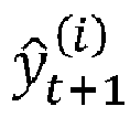
- In the following, the results are presented. Each experiment is discussed separately. First, the individual performance assessment is assessed. In this subsection, the aim is to assess the isolated performance of each prediction algorithm. To this end, the performance metrics discussed above are used. The values obtained for the RMSE and MAPE metrics are summarized in
Fig. 4a . For the comparison of the retrieved prediction performances, the naive method was used as benchmark. It is only outperformed by the ARIMA algorithm in matters of the MAPE. The MAPE improvement achieved by ARIMA is 8 %. These superior results are achieved due to the integration part of ARIMA. Thus, the algorithm can better adjust itself to the non-stationary data. It is also relevant to mention that all considered algorithms except for BATS and TBATS achieved an average prediction error rate of less than 5%. However, the comparison with regard to the RMSE retrieves better results. ARIMA, BATS and TBATS outperform the benchmark. Especially BATS and TBATS achieve much better results. Their good RMSE results are interesting, because they both obtained relatively high MAPE values with respectively 7.47 % and 7.48 %. The other naive method, Random Walk, and the Exponential Smoothing Algorithms achieve comparable results like the benchmark. The discrepancies obtained both in terms of RMSE and MAPE hint that combining the forecasts of several algorithms might result in an improvement of the overall performance.Fig. 4a shows an overview of the prediction performance scores obtained by the algorithms on the test set. - The table shown in
Fig. 4b extends the results described inFig. 4a to cover computational aspects. As discussed above, computational complexity and run-time requirements may be deemed critical to the objective of predicting HV current measurements. Considering the prediction horizon of below 20 time-steps, the methods of seasonal ARIMA, BATS and TBATS may be deemed obsolete. Their respective run-time may exceed our limit of at maximum 200 ms. Under real usage conditions, the obtained forecasts may be irrelevant by the time they are computed. ARIMA misses the run-time limit only shortly. Further optimizations may make this algorithm feasible for the purposes. Without further optimizations, the focus may be set on the remaining simplest methods for deployment.Fig. 4b shows a comparison per algorithm with regard to accuracy and efficiency. - In this section, the results obtained during bootstrap aggregation. For this experiment, the five algorithms with the lowest MAPE were combined. Thus, the algorithms considered for the combination are ARIMA, the simple and Holt-Winters Exponential Smoothing, as well as the Random Walk and the naive method, as can be seen from
Fig. 4a . As mentioned above, an equal weights approach was followed. The prediction values of each algorithm are therefore averaged at each prediction run-through. The hereby discussed results are obtained for the same data sets used above. This enables an objective comparison of the individual and combined performances on the same data. For the same test set, the bootstrap aggregation resulted in an RMSE value of 1.74 and a MAPE value of 4.19 %. This means again a prediction error rate of below 5 %. Compared to the individual performances, the bootstrap aggregation outperformed all individual methods in terms of the MAPE except for ARIMA. Accordingly, bootstrap aggregation fails to improve the overall prediction. Nevertheless, the results may be improved with an adaptive weights approach. Instead of the equal weights approach used in the context of the present disclosure, the adaptive weights approach might be able to benefit from the high accuracy of ARIMA. - As expected, Bootstrap Aggregation has the worst runtime of all considered approaches. As the concept combines the predictions of several algorithms, it also sums up the required run-time of all these algorithms. Especially in the application field outlined above, the execution on ECUs, the long runtime may be considered a disadvantage. Regrettably, this disadvantage might not be equalized by the achieved results.
- Time delays between distributed systems lead to outdated measurement signals. But up-to-date input data is required for control functions, especially in real-time systems like power trains of EVs. A solution to this problem is to predict delayed signals until the present. The goal of this paper is to evaluate which algorithms are suited for time series prediction of delayed measurement signals of power trains of EVs. For this purpose, we evaluate 5 state-of-the-art time series prediction algorithms and 2 naive methods. As it is important for real-time systems to retrieve information in the required time frame, we focus our evaluation not only on accuracy which we measure with the RMSE and the MAPE, but also on the required run-time to execute the prediction. BATS and TBATS are the most accurate algorithms. However, due to their high outliers, they are unsuited for our purposes. ARIMA offers the best compromise between high accuracy and small outliers. As expected, the naive method is the fastest method. Surprisingly, although it is the simplest of all methods, its accuracy is not far below the other methods. Its relatively good results show the difficulty of predicting HV measurements of electric power trains accurately. Thus, further work needs to be done to enable fast and accurate predictions. A possibility for future work is to optimize ARIMA and try to make it faster. Another possibility is to combine the predictions of several algorithms with Bootstrap Aggregation. Although the here implemented equal weights approach outper-forms almost all algorithms, it is not able to achieve the low MAPE value of ARIMA. Further work is necessary to investigate, if an adaptive weights approach is able to outperform ARIMA. Until now, Bootstrap Aggregation requires by far the most run-time.
- The aspects and features mentioned and described together with one or more of the previously detailed examples and figures, may as well be combined with one or more of the other examples in order to replace a like feature of the other example or in order to additionally introduce the feature to the other example.
- Examples may further be or relate to a computer program having a program code for performing one or more of the above methods, when the computer program is executed on a computer or processor. Steps, operations or processes of various above-described methods may be performed by programmed computers or processors. Examples may also cover program storage devices such as digital data storage media, which are machine, processor or computer readable and encode machine-executable, processor-executable or computer-executable programs of instructions. The instructions perform or cause performing some or all of the acts of the above-described methods. The program storage devices may comprise or be, for instance, digital memories, magnetic storage media such as magnetic disks and magnetic tapes, hard drives, or optically readable digital data storage media. Further examples may also cover computers, processors or control units programmed to perform the acts of the above-described methods or (field) programmable logic arrays ((F)PLAs) or (field) programmable gate arrays ((F)PGAs), programmed to perform the acts of the above-described methods.
- The description and drawings merely illustrate the principles of the disclosure. Furthermore, all examples recited herein are principally intended expressly to be only for illustrative purposes to aid the reader in understanding the principles of the disclosure and the concepts contributed by the inventor(s) to furthering the art. All statements herein reciting principles, aspects, and examples of the disclosure, as well as specific examples thereof, are intended to encompass equivalents thereof.
- A functional block denoted as "means for ..." performing a certain function may refer to a circuit that is configured to perform a certain function. Hence, a "means for s.th." may be implemented as a "means configured to or suited for s.th.", such as a device or a circuit configured to or suited for the respective task.
- Functions of various elements shown in the figures, including any functional blocks labeled as "means", "means for providing a signal", "means for generating a signal.", etc., may be implemented in the form of dedicated hardware, such as "a signal provider", "a signal processing unit", "a processor", "a controller", etc. as well as hardware capable of executing software in association with appropriate software. When provided by a processor, the functions may be provided by a single dedicated processor, by a single shared processor, or by a plurality of individual processors, some of which or all of which may be shared. However, the term "processor" or "controller" is by far not limited to hardware exclusively capable of executing software, but may include digital signal processor (DSP) hardware, network processor, application specific integrated circuit (ASIC), field programmable gate array (FPGA), read only memory (ROM) for storing software, random access memory (RAM), and nonvolatile storage. Other hardware, conventional and/or custom, may also be included.
- A block diagram may, for instance, illustrate a high-level circuit diagram implementing the principles of the disclosure. Similarly, a flow chart, a flow diagram, a state transition diagram, a pseudo code, and the like may represent various processes, operations or steps, which may, for instance, be substantially represented in computer readable medium and so executed by a computer or processor, whether or not such computer or processor is explicitly shown. Methods disclosed in the specification or in the claims may be implemented by a device having means for performing each of the respective acts of these methods.
- It is to be understood that the disclosure of multiple acts, processes, operations, steps or functions disclosed in the specification or claims may not be construed as to be within the specific order, unless explicitly or implicitly stated otherwise, for instance for technical reasons. Therefore, the disclosure of multiple acts or functions will not limit these to a particular order unless such acts or functions are not interchangeable for technical reasons. Furthermore, in some examples a single act, function, process, operation or step may include or may be broken into multiple sub-acts, -functions, -processes, -operations or -steps, respectively. Such sub acts may be included and part of the disclosure of this single act unless explicitly excluded.
- Furthermore, the following claims are hereby incorporated into the detailed description, where each claim may stand on its own as a separate example. While each claim may stand on its own as a separate example, it is to be noted that - although a dependent claim may refer in the claims to a specific combination with one or more other claims - other examples may also include a combination of the dependent claim with the subject matter of each other dependent or independent claim. Such combinations are explicitly proposed herein unless it is stated that a specific combination is not intended. Furthermore, it is intended to include also features of a claim to any other independent claim even if this claim is not directly made dependent to the independent claim.
Claims (15)
- A system (10) for determining estimated sensor data of a sensor (20), the system comprising processing circuitry (14) configured to:obtain a plurality of samples of sensor data of the sensor (20);obtain information on a time offset between the sensor data of the sensor and a reference time;perform a time-series projection based on the plurality of samples of the sensor data, the time-series projection being performed using an auto-regressive statistical model;determine an estimate of the sensor data for the reference time based on the time-series projection and based on the time offset between the sensor data and the reference time.
- The system according to claim 1, wherein the auto-regressive statistical model is an auto-regressive moving average-model.
- The system according to one of the claims 1 or 2, wherein the auto-regressive model is applied on a differentiation of the plurality of samples of the sensor data.
- The system according to claim 3, wherein the auto-regressive model is applied on a once-derived version of the plurality of samples of the sensor data.
- The system according to one of the claims 1 to 4, wherein the auto-regressive model is one of an Autoregressive Integrated Moving Average, ARIMA, or an Autoregressive Moving Average, ARMA, model.
- The system according to one of the claims 1 to 5, wherein the time-series projection is performed using at least 20 samples and/or at most 60 samples of the sensor data of the sensor.
- The system according to one of the claims 1 to 6, wherein the sensor data of the sensor relates to a current of a power train of an electric vehicle (100).
- The system according to one of the claims 1 to 7, wherein the processing circuitry is configured to perform the time-series projection such, that the time offset between the sensor data and the reference time is bridged by the time-series projection.
- The system according to claim 8, wherein the processing circuitry is configured to output the estimate of the sensor data.
- The system according to one of the claims 1 to 9, wherein the processing circuitry is configured to perform the time-series projection with a projection horizon that matches the time offset between the sensor data and the reference time.
- The system according to one of the claims 1 to 10, wherein the reference time is based on sensor data of a second sensor (30), the sensor data of the second sensor comprising a second plurality of samples, wherein the processing circuitry is configured to determine the estimate of the sensor data such, that the estimate of the sensor data is time-synchronized to the latest sample of the sensor data of the second sensor.
- The system according to claim 11, wherein the processing circuitry is configured to obtain the sensor data of the second sensor, and to derive the time offset between the sensor data of the sensor and the reference time based on the sensor data of the second sensor and based on the sensor data of the sensor.
- The system according to one of the claims 11 or 12, wherein the processing circuitry is configured to obtain the sensor data of the second sensor, wherein the processing circuitry is configured to output time-synchronized versions of the estimated sensor data of the sensor and of the sensor data of the second sensor.
- A method for determining estimated sensor data, the method comprising:obtaining (110) a plurality of samples of sensor data of a sensor;obtaining (120) information on a time offset between the sensor data of the sensor and a reference time;performing (130) a time-series projection based on the plurality of samples of the sensor data, the time-series projection being performed using an auto-regressive statistical model;determining (140) an estimate of the sensor data for the reference time based on the time-series projection and based on the time offset between the sensor data and the reference time.
- A computer program having a program code for performing the method of claim 14, when the computer program is executed on a computer, a processor, or a programmable hardware component.
Priority Applications (4)
| Application Number | Priority Date | Filing Date | Title |
|---|---|---|---|
| EP20171463.1A EP3904172B1 (en) | 2020-04-27 | 2020-04-27 | System, method and computer program for determining estimated sensor data |
| CN202180025666.0A CN115362093B (en) | 2020-04-27 | 2021-02-02 | Systems, methods, and computer programs for determining estimated sensor data |
| US17/916,965 US12526123B2 (en) | 2020-04-27 | 2021-02-02 | System, method and computer program for determining estimated sensor data |
| PCT/EP2021/052359 WO2021219259A1 (en) | 2020-04-27 | 2021-02-02 | System, method and computer program for determining estimated sensor data |
Applications Claiming Priority (1)
| Application Number | Priority Date | Filing Date | Title |
|---|---|---|---|
| EP20171463.1A EP3904172B1 (en) | 2020-04-27 | 2020-04-27 | System, method and computer program for determining estimated sensor data |
Publications (2)
| Publication Number | Publication Date |
|---|---|
| EP3904172A1 true EP3904172A1 (en) | 2021-11-03 |
| EP3904172B1 EP3904172B1 (en) | 2024-07-31 |
Family
ID=70464952
Family Applications (1)
| Application Number | Title | Priority Date | Filing Date |
|---|---|---|---|
| EP20171463.1A Active EP3904172B1 (en) | 2020-04-27 | 2020-04-27 | System, method and computer program for determining estimated sensor data |
Country Status (4)
| Country | Link |
|---|---|
| US (1) | US12526123B2 (en) |
| EP (1) | EP3904172B1 (en) |
| CN (1) | CN115362093B (en) |
| WO (1) | WO2021219259A1 (en) |
Cited By (3)
| Publication number | Priority date | Publication date | Assignee | Title |
|---|---|---|---|---|
| CN117118510A (en) * | 2023-10-12 | 2023-11-24 | 湖北经济学院 | A machine learning-based optical channel bit error rate prediction method |
| WO2025242285A1 (en) * | 2024-05-21 | 2025-11-27 | Abb Schweiz Ag | A method for an industrial object in an industrial system |
| WO2025242289A1 (en) * | 2024-05-21 | 2025-11-27 | Abb Schweiz Ag | A method for an industrial object in an industrial system |
Families Citing this family (2)
| Publication number | Priority date | Publication date | Assignee | Title |
|---|---|---|---|---|
| CN116361620B (en) * | 2023-06-02 | 2023-08-29 | 西安麦仁网络科技有限公司 | A method for intelligent processing of chip data |
| EP4675497A1 (en) * | 2024-07-02 | 2026-01-07 | Volkswagen Aktiengesellschaft | Method for providing representative load profiles, control unit and vehicle |
Citations (1)
| Publication number | Priority date | Publication date | Assignee | Title |
|---|---|---|---|---|
| US20120239241A1 (en) * | 2011-03-18 | 2012-09-20 | Robert Bosch Gmbh | Yaw rate forecasting |
Family Cites Families (10)
| Publication number | Priority date | Publication date | Assignee | Title |
|---|---|---|---|---|
| US6755266B2 (en) * | 2000-10-31 | 2004-06-29 | Volvo Car Corporation | Method and arrangement in a hybrid vehicle for initiating early engine operation during take-off conditions |
| US7921317B2 (en) * | 2008-09-02 | 2011-04-05 | Unisys Corporation | Method and apparatus for synchronizing central processing units in a multiprocessor apparatus |
| CN104011563B (en) * | 2011-10-24 | 2016-08-17 | 大陆-特韦斯贸易合伙股份公司及两合公司 | Sensing system for its data precision of independent assessment |
| WO2018065061A1 (en) * | 2016-10-06 | 2018-04-12 | Huawei Technologies Co., Ltd. | Receiver and method for compensating a frequency error in a reference clock |
| IT201600130103A1 (en) * | 2016-12-22 | 2018-06-22 | St Microelectronics Srl | SKEW COMPENSATION PROCEDURE FOR CLOCK AND ITS SYSTEM |
| EP3638557A4 (en) * | 2017-05-10 | 2021-02-24 | The Regents of The University of Michigan | FAULT DETECTION AND REACTION |
| EP3438776B1 (en) * | 2017-08-04 | 2022-09-07 | Bayerische Motoren Werke Aktiengesellschaft | Method, apparatus and computer program for a vehicle |
| US10800427B2 (en) * | 2017-10-19 | 2020-10-13 | Uatc, Llc | Systems and methods for a vehicle controller robust to time delays |
| US10773666B2 (en) * | 2018-05-08 | 2020-09-15 | Infineon Technologies Ag | High speed sensor interface |
| EP3815045B1 (en) * | 2018-06-29 | 2025-10-22 | Zoox, Inc. | Sensor calibration |
-
2020
- 2020-04-27 EP EP20171463.1A patent/EP3904172B1/en active Active
-
2021
- 2021-02-02 WO PCT/EP2021/052359 patent/WO2021219259A1/en not_active Ceased
- 2021-02-02 CN CN202180025666.0A patent/CN115362093B/en active Active
- 2021-02-02 US US17/916,965 patent/US12526123B2/en active Active
Patent Citations (1)
| Publication number | Priority date | Publication date | Assignee | Title |
|---|---|---|---|---|
| US20120239241A1 (en) * | 2011-03-18 | 2012-09-20 | Robert Bosch Gmbh | Yaw rate forecasting |
Non-Patent Citations (9)
| Title |
|---|
| A. M. DE LIVERAR. J. HYNDMANR. D. SNYDER, FORECASTING TIME SERIES WITH COMPLEX SEASONAL PATTERNS USING EXPONENTIAL SMOOTHING, 2011 |
| C. BERGMEIRJ. BENTEZ, ON THE USE OF CROSS-VALIDATION FOR TIME SERIES PREDICTOR EVALUATION, 2012 |
| C. BERGMEIRR. J. HYNDMANJ. M. BENITEZ, BAGGING EXPONENTIAL SMOOTHING METHODS USING STL DECOMPOSITION AND BOX-COX TRANSFORMATION, 2016 |
| J. PFEIFFERX. WU, AUTOMATED TIME DELAY ESTIMATION FOR DISTRIBUTED SENSOR SYSTEMS OF ELECTRIC VEHICLES, 2019 |
| L. J. TASHMAN, OUT-OF-SAMPLE TESTS OF FORECASTING ACCURACY: AN ANALYSIS AND REVIEW, 2000 |
| O. GJOL-BERGB.-A. BENGTSSON, FORECASTING QUARTERLY HOG PRICES: SIMPLE AUTOREGRESSIVE MODELS VS. NAIVE PREDICTIONS, 1997 |
| R. G. BROWNA. D. LITTLE, EXPONENTIAL SMOOTHING FOR PREDICTING DEMAND, 1956 |
| R. J. HYNDMANY. KHANDAKAR, AUTOMATIC TIME SERIES FORECASTING: THE FORECAST PACKAGE FOR R, 2008 |
| V. KOTUB. DESHPANDE: "Data Science: Concepts and Practice", 2019, ELSEVIER |
Cited By (4)
| Publication number | Priority date | Publication date | Assignee | Title |
|---|---|---|---|---|
| CN117118510A (en) * | 2023-10-12 | 2023-11-24 | 湖北经济学院 | A machine learning-based optical channel bit error rate prediction method |
| CN117118510B (en) * | 2023-10-12 | 2023-12-22 | 湖北经济学院 | Optical channel error rate prediction method based on machine learning |
| WO2025242285A1 (en) * | 2024-05-21 | 2025-11-27 | Abb Schweiz Ag | A method for an industrial object in an industrial system |
| WO2025242289A1 (en) * | 2024-05-21 | 2025-11-27 | Abb Schweiz Ag | A method for an industrial object in an industrial system |
Also Published As
| Publication number | Publication date |
|---|---|
| CN115362093B (en) | 2025-08-12 |
| EP3904172B1 (en) | 2024-07-31 |
| US12526123B2 (en) | 2026-01-13 |
| CN115362093A (en) | 2022-11-18 |
| WO2021219259A1 (en) | 2021-11-04 |
| US20230140907A1 (en) | 2023-05-11 |
Similar Documents
| Publication | Publication Date | Title |
|---|---|---|
| EP3904172B1 (en) | System, method and computer program for determining estimated sensor data | |
| Arandia et al. | Tailoring seasonal time series models to forecast short-term water demand | |
| Pandey et al. | Hybrid models for water demand forecasting | |
| CN102042848B (en) | Prediction method of multi-functional parameter accelerated degradation testing product life based on multivariate hybrid time sequence analysis | |
| Koukaras et al. | Introducing a novel approach in one-step ahead energy load forecasting | |
| CN112148557B (en) | Method for predicting performance index in real time, computer equipment and storage medium | |
| Saini et al. | A novel probabilistic gradient boosting model with multi-approach feature selection and iterative seasonal trend decomposition for short-term load forecasting | |
| Ayala Solares et al. | Nonlinear model structure detection and parameter estimation using a novel bagging method based on distance correlation metric | |
| CN103793613A (en) | Degradation data missing interpolation method based on regression analysis and RBF neural network | |
| Ketabi et al. | Vehicular traffic density forecasting through the eyes of traffic cameras; a spatio-temporal machine learning study | |
| CN106056239A (en) | Product inventory predicting method and product inventory predicting device | |
| CN118693809A (en) | Day-ahead load forecasting method and device based on CVAE and GPT | |
| Guo et al. | A hybrid residual correction method with auxiliary particle filter and conditional kernel density estimation for remaining useful life prediction | |
| Kissi et al. | Forecasting construction tender price index in Ghana using autoregressive integrated moving average with exogenous variables model | |
| Lee et al. | Very short-Term wind power ensemble forecasting without numerical weather prediction through the predictor design | |
| CN115564466A (en) | A two-tier day-ahead electricity price forecasting method with calibration window integration and coupling market characteristics | |
| Zhang et al. | Method of speed data fusion based on Bayesian combination algorithm and high‐order multi‐variable Markov model | |
| Li et al. | Reducing reinforcement learning to KWIK online regression | |
| Lin et al. | Cloud-based vehicle velocity prediction based on seasonal autoregressive integrated moving average processes | |
| Nikseresht et al. | Adaptive stochastic modeling of nonlinear time series: ARFIMA meets improved fractional Ornstein-Uhlenbeck | |
| Wang et al. | Health indicator forecasting for improving remaining useful life estimation | |
| Wang et al. | Bayesian analysis for NHPP-based software fault detection and correction processes | |
| Pfeiffer et al. | Time Series Prediction for Measurements of Electric Power Trains | |
| Wei et al. | Safety detection and risk early warning model for bridge health monitoring based on neural network algorithm | |
| Jiang et al. | Traffic Flow Prediction: A Hybrid VMD-NRBO-BiLSTM Model Approach |
Legal Events
| Date | Code | Title | Description |
|---|---|---|---|
| PUAI | Public reference made under article 153(3) epc to a published international application that has entered the european phase |
Free format text: ORIGINAL CODE: 0009012 |
|
| STAA | Information on the status of an ep patent application or granted ep patent |
Free format text: STATUS: THE APPLICATION HAS BEEN PUBLISHED |
|
| AK | Designated contracting states |
Kind code of ref document: A1 Designated state(s): AL AT BE BG CH CY CZ DE DK EE ES FI FR GB GR HR HU IE IS IT LI LT LU LV MC MK MT NL NO PL PT RO RS SE SI SK SM TR |
|
| B565 | Issuance of search results under rule 164(2) epc |
Effective date: 20201019 |
|
| STAA | Information on the status of an ep patent application or granted ep patent |
Free format text: STATUS: REQUEST FOR EXAMINATION WAS MADE |
|
| 17P | Request for examination filed |
Effective date: 20220221 |
|
| RBV | Designated contracting states (corrected) |
Designated state(s): AL AT BE BG CH CY CZ DE DK EE ES FI FR GB GR HR HU IE IS IT LI LT LU LV MC MK MT NL NO PL PT RO RS SE SI SK SM TR |
|
| P01 | Opt-out of the competence of the unified patent court (upc) registered |
Effective date: 20230502 |
|
| GRAP | Despatch of communication of intention to grant a patent |
Free format text: ORIGINAL CODE: EPIDOSNIGR1 |
|
| STAA | Information on the status of an ep patent application or granted ep patent |
Free format text: STATUS: GRANT OF PATENT IS INTENDED |
|
| INTG | Intention to grant announced |
Effective date: 20240416 |
|
| P02 | Opt-out of the competence of the unified patent court (upc) changed |
Effective date: 20240502 |
|
| GRAS | Grant fee paid |
Free format text: ORIGINAL CODE: EPIDOSNIGR3 |
|
| GRAA | (expected) grant |
Free format text: ORIGINAL CODE: 0009210 |
|
| STAA | Information on the status of an ep patent application or granted ep patent |
Free format text: STATUS: THE PATENT HAS BEEN GRANTED |
|
| AK | Designated contracting states |
Kind code of ref document: B1 Designated state(s): AL AT BE BG CH CY CZ DE DK EE ES FI FR GB GR HR HU IE IS IT LI LT LU LV MC MK MT NL NO PL PT RO RS SE SI SK SM TR |
|
| REG | Reference to a national code |
Ref country code: CH Ref legal event code: EP Ref country code: GB Ref legal event code: FG4D |
|
| REG | Reference to a national code |
Ref country code: DE Ref legal event code: R096 Ref document number: 602020034727 Country of ref document: DE |
|
| REG | Reference to a national code |
Ref country code: IE Ref legal event code: FG4D |
|
| REG | Reference to a national code |
Ref country code: LT Ref legal event code: MG9D |
|
| REG | Reference to a national code |
Ref country code: NL Ref legal event code: MP Effective date: 20240731 |
|
| PG25 | Lapsed in a contracting state [announced via postgrant information from national office to epo] |
Ref country code: PT Free format text: LAPSE BECAUSE OF FAILURE TO SUBMIT A TRANSLATION OF THE DESCRIPTION OR TO PAY THE FEE WITHIN THE PRESCRIBED TIME-LIMIT Effective date: 20241202 |
|
| REG | Reference to a national code |
Ref country code: AT Ref legal event code: MK05 Ref document number: 1708201 Country of ref document: AT Kind code of ref document: T Effective date: 20240731 |
|
| PG25 | Lapsed in a contracting state [announced via postgrant information from national office to epo] |
Ref country code: PT Free format text: LAPSE BECAUSE OF FAILURE TO SUBMIT A TRANSLATION OF THE DESCRIPTION OR TO PAY THE FEE WITHIN THE PRESCRIBED TIME-LIMIT Effective date: 20241202 |
|
| PG25 | Lapsed in a contracting state [announced via postgrant information from national office to epo] |
Ref country code: NO Free format text: LAPSE BECAUSE OF FAILURE TO SUBMIT A TRANSLATION OF THE DESCRIPTION OR TO PAY THE FEE WITHIN THE PRESCRIBED TIME-LIMIT Effective date: 20241031 |
|
| PG25 | Lapsed in a contracting state [announced via postgrant information from national office to epo] |
Ref country code: GR Free format text: LAPSE BECAUSE OF FAILURE TO SUBMIT A TRANSLATION OF THE DESCRIPTION OR TO PAY THE FEE WITHIN THE PRESCRIBED TIME-LIMIT Effective date: 20241101 Ref country code: FI Free format text: LAPSE BECAUSE OF FAILURE TO SUBMIT A TRANSLATION OF THE DESCRIPTION OR TO PAY THE FEE WITHIN THE PRESCRIBED TIME-LIMIT Effective date: 20240731 Ref country code: NL Free format text: LAPSE BECAUSE OF FAILURE TO SUBMIT A TRANSLATION OF THE DESCRIPTION OR TO PAY THE FEE WITHIN THE PRESCRIBED TIME-LIMIT Effective date: 20240731 Ref country code: PL Free format text: LAPSE BECAUSE OF FAILURE TO SUBMIT A TRANSLATION OF THE DESCRIPTION OR TO PAY THE FEE WITHIN THE PRESCRIBED TIME-LIMIT Effective date: 20240731 |
|
| PG25 | Lapsed in a contracting state [announced via postgrant information from national office to epo] |
Ref country code: BG Free format text: LAPSE BECAUSE OF FAILURE TO SUBMIT A TRANSLATION OF THE DESCRIPTION OR TO PAY THE FEE WITHIN THE PRESCRIBED TIME-LIMIT Effective date: 20240731 |
|
| PG25 | Lapsed in a contracting state [announced via postgrant information from national office to epo] |
Ref country code: LV Free format text: LAPSE BECAUSE OF FAILURE TO SUBMIT A TRANSLATION OF THE DESCRIPTION OR TO PAY THE FEE WITHIN THE PRESCRIBED TIME-LIMIT Effective date: 20240731 |
|
| PG25 | Lapsed in a contracting state [announced via postgrant information from national office to epo] |
Ref country code: IS Free format text: LAPSE BECAUSE OF FAILURE TO SUBMIT A TRANSLATION OF THE DESCRIPTION OR TO PAY THE FEE WITHIN THE PRESCRIBED TIME-LIMIT Effective date: 20241130 Ref country code: AT Free format text: LAPSE BECAUSE OF FAILURE TO SUBMIT A TRANSLATION OF THE DESCRIPTION OR TO PAY THE FEE WITHIN THE PRESCRIBED TIME-LIMIT Effective date: 20240731 |
|
| PG25 | Lapsed in a contracting state [announced via postgrant information from national office to epo] |
Ref country code: HR Free format text: LAPSE BECAUSE OF FAILURE TO SUBMIT A TRANSLATION OF THE DESCRIPTION OR TO PAY THE FEE WITHIN THE PRESCRIBED TIME-LIMIT Effective date: 20240731 |
|
| PG25 | Lapsed in a contracting state [announced via postgrant information from national office to epo] |
Ref country code: ES Free format text: LAPSE BECAUSE OF FAILURE TO SUBMIT A TRANSLATION OF THE DESCRIPTION OR TO PAY THE FEE WITHIN THE PRESCRIBED TIME-LIMIT Effective date: 20240731 Ref country code: RS Free format text: LAPSE BECAUSE OF FAILURE TO SUBMIT A TRANSLATION OF THE DESCRIPTION OR TO PAY THE FEE WITHIN THE PRESCRIBED TIME-LIMIT Effective date: 20241031 |
|
| PG25 | Lapsed in a contracting state [announced via postgrant information from national office to epo] |
Ref country code: RS Free format text: LAPSE BECAUSE OF FAILURE TO SUBMIT A TRANSLATION OF THE DESCRIPTION OR TO PAY THE FEE WITHIN THE PRESCRIBED TIME-LIMIT Effective date: 20241031 Ref country code: PL Free format text: LAPSE BECAUSE OF FAILURE TO SUBMIT A TRANSLATION OF THE DESCRIPTION OR TO PAY THE FEE WITHIN THE PRESCRIBED TIME-LIMIT Effective date: 20240731 Ref country code: NO Free format text: LAPSE BECAUSE OF FAILURE TO SUBMIT A TRANSLATION OF THE DESCRIPTION OR TO PAY THE FEE WITHIN THE PRESCRIBED TIME-LIMIT Effective date: 20241031 Ref country code: NL Free format text: LAPSE BECAUSE OF FAILURE TO SUBMIT A TRANSLATION OF THE DESCRIPTION OR TO PAY THE FEE WITHIN THE PRESCRIBED TIME-LIMIT Effective date: 20240731 Ref country code: LV Free format text: LAPSE BECAUSE OF FAILURE TO SUBMIT A TRANSLATION OF THE DESCRIPTION OR TO PAY THE FEE WITHIN THE PRESCRIBED TIME-LIMIT Effective date: 20240731 Ref country code: IS Free format text: LAPSE BECAUSE OF FAILURE TO SUBMIT A TRANSLATION OF THE DESCRIPTION OR TO PAY THE FEE WITHIN THE PRESCRIBED TIME-LIMIT Effective date: 20241130 Ref country code: HR Free format text: LAPSE BECAUSE OF FAILURE TO SUBMIT A TRANSLATION OF THE DESCRIPTION OR TO PAY THE FEE WITHIN THE PRESCRIBED TIME-LIMIT Effective date: 20240731 Ref country code: GR Free format text: LAPSE BECAUSE OF FAILURE TO SUBMIT A TRANSLATION OF THE DESCRIPTION OR TO PAY THE FEE WITHIN THE PRESCRIBED TIME-LIMIT Effective date: 20241101 Ref country code: FI Free format text: LAPSE BECAUSE OF FAILURE TO SUBMIT A TRANSLATION OF THE DESCRIPTION OR TO PAY THE FEE WITHIN THE PRESCRIBED TIME-LIMIT Effective date: 20240731 Ref country code: ES Free format text: LAPSE BECAUSE OF FAILURE TO SUBMIT A TRANSLATION OF THE DESCRIPTION OR TO PAY THE FEE WITHIN THE PRESCRIBED TIME-LIMIT Effective date: 20240731 Ref country code: BG Free format text: LAPSE BECAUSE OF FAILURE TO SUBMIT A TRANSLATION OF THE DESCRIPTION OR TO PAY THE FEE WITHIN THE PRESCRIBED TIME-LIMIT Effective date: 20240731 Ref country code: AT Free format text: LAPSE BECAUSE OF FAILURE TO SUBMIT A TRANSLATION OF THE DESCRIPTION OR TO PAY THE FEE WITHIN THE PRESCRIBED TIME-LIMIT Effective date: 20240731 |
|
| PG25 | Lapsed in a contracting state [announced via postgrant information from national office to epo] |
Ref country code: DK Free format text: LAPSE BECAUSE OF FAILURE TO SUBMIT A TRANSLATION OF THE DESCRIPTION OR TO PAY THE FEE WITHIN THE PRESCRIBED TIME-LIMIT Effective date: 20240731 Ref country code: RO Free format text: LAPSE BECAUSE OF FAILURE TO SUBMIT A TRANSLATION OF THE DESCRIPTION OR TO PAY THE FEE WITHIN THE PRESCRIBED TIME-LIMIT Effective date: 20240731 Ref country code: SM Free format text: LAPSE BECAUSE OF FAILURE TO SUBMIT A TRANSLATION OF THE DESCRIPTION OR TO PAY THE FEE WITHIN THE PRESCRIBED TIME-LIMIT Effective date: 20240731 |
|
| PG25 | Lapsed in a contracting state [announced via postgrant information from national office to epo] |
Ref country code: EE Free format text: LAPSE BECAUSE OF FAILURE TO SUBMIT A TRANSLATION OF THE DESCRIPTION OR TO PAY THE FEE WITHIN THE PRESCRIBED TIME-LIMIT Effective date: 20240731 |
|
| PG25 | Lapsed in a contracting state [announced via postgrant information from national office to epo] |
Ref country code: CZ Free format text: LAPSE BECAUSE OF FAILURE TO SUBMIT A TRANSLATION OF THE DESCRIPTION OR TO PAY THE FEE WITHIN THE PRESCRIBED TIME-LIMIT Effective date: 20240731 |
|
| PG25 | Lapsed in a contracting state [announced via postgrant information from national office to epo] |
Ref country code: IT Free format text: LAPSE BECAUSE OF FAILURE TO SUBMIT A TRANSLATION OF THE DESCRIPTION OR TO PAY THE FEE WITHIN THE PRESCRIBED TIME-LIMIT Effective date: 20240731 Ref country code: SK Free format text: LAPSE BECAUSE OF FAILURE TO SUBMIT A TRANSLATION OF THE DESCRIPTION OR TO PAY THE FEE WITHIN THE PRESCRIBED TIME-LIMIT Effective date: 20240731 |
|
| REG | Reference to a national code |
Ref country code: DE Ref legal event code: R097 Ref document number: 602020034727 Country of ref document: DE |
|
| PLBE | No opposition filed within time limit |
Free format text: ORIGINAL CODE: 0009261 |
|
| STAA | Information on the status of an ep patent application or granted ep patent |
Free format text: STATUS: NO OPPOSITION FILED WITHIN TIME LIMIT |
|
| 26N | No opposition filed |
Effective date: 20250501 |
|
| PGFP | Annual fee paid to national office [announced via postgrant information from national office to epo] |
Ref country code: DE Payment date: 20250408 Year of fee payment: 6 |
|
| PG25 | Lapsed in a contracting state [announced via postgrant information from national office to epo] |
Ref country code: SE Free format text: LAPSE BECAUSE OF FAILURE TO SUBMIT A TRANSLATION OF THE DESCRIPTION OR TO PAY THE FEE WITHIN THE PRESCRIBED TIME-LIMIT Effective date: 20240731 |
|
| REG | Reference to a national code |
Ref country code: CH Ref legal event code: H13 Free format text: ST27 STATUS EVENT CODE: U-0-0-H10-H13 (AS PROVIDED BY THE NATIONAL OFFICE) Effective date: 20251125 |
|
| PG25 | Lapsed in a contracting state [announced via postgrant information from national office to epo] |
Ref country code: LU Free format text: LAPSE BECAUSE OF NON-PAYMENT OF DUE FEES Effective date: 20250427 |
|
| PG25 | Lapsed in a contracting state [announced via postgrant information from national office to epo] |
Ref country code: MC Free format text: LAPSE BECAUSE OF FAILURE TO SUBMIT A TRANSLATION OF THE DESCRIPTION OR TO PAY THE FEE WITHIN THE PRESCRIBED TIME-LIMIT Effective date: 20240731 |
|
| GBPC | Gb: european patent ceased through non-payment of renewal fee |
Effective date: 20250427 |
|
| REG | Reference to a national code |
Ref country code: BE Ref legal event code: MM Effective date: 20250430 |
|
| PG25 | Lapsed in a contracting state [announced via postgrant information from national office to epo] |
Ref country code: GB Free format text: LAPSE BECAUSE OF NON-PAYMENT OF DUE FEES Effective date: 20250427 |
|
| PG25 | Lapsed in a contracting state [announced via postgrant information from national office to epo] |
Ref country code: FR Free format text: LAPSE BECAUSE OF NON-PAYMENT OF DUE FEES Effective date: 20250430 |
|
| PG25 | Lapsed in a contracting state [announced via postgrant information from national office to epo] |
Ref country code: BE Free format text: LAPSE BECAUSE OF NON-PAYMENT OF DUE FEES Effective date: 20250430 |
|
| PG25 | Lapsed in a contracting state [announced via postgrant information from national office to epo] |
Ref country code: CH Free format text: LAPSE BECAUSE OF NON-PAYMENT OF DUE FEES Effective date: 20250430 |
|
| PG25 | Lapsed in a contracting state [announced via postgrant information from national office to epo] |
Ref country code: IE Free format text: LAPSE BECAUSE OF NON-PAYMENT OF DUE FEES Effective date: 20250427 |