EP3731154A1 - Training a convolutional neural network for image retrieval with a listwise ranking loss function - Google Patents
Training a convolutional neural network for image retrieval with a listwise ranking loss function Download PDFInfo
- Publication number
- EP3731154A1 EP3731154A1 EP19305542.3A EP19305542A EP3731154A1 EP 3731154 A1 EP3731154 A1 EP 3731154A1 EP 19305542 A EP19305542 A EP 19305542A EP 3731154 A1 EP3731154 A1 EP 3731154A1
- Authority
- EP
- European Patent Office
- Prior art keywords
- images
- ranking
- cnn
- batch
- image
- Prior art date
- Legal status (The legal status is an assumption and is not a legal conclusion. Google has not performed a legal analysis and makes no representation as to the accuracy of the status listed.)
- Pending
Links
Images


Classifications
-
- G—PHYSICS
- G06—COMPUTING OR CALCULATING; COUNTING
- G06N—COMPUTING ARRANGEMENTS BASED ON SPECIFIC COMPUTATIONAL MODELS
- G06N3/00—Computing arrangements based on biological models
- G06N3/02—Neural networks
- G06N3/08—Learning methods
- G06N3/084—Backpropagation, e.g. using gradient descent
-
- G—PHYSICS
- G06—COMPUTING OR CALCULATING; COUNTING
- G06F—ELECTRIC DIGITAL DATA PROCESSING
- G06F16/00—Information retrieval; Database structures therefor; File system structures therefor
- G06F16/50—Information retrieval; Database structures therefor; File system structures therefor of still image data
- G06F16/56—Information retrieval; Database structures therefor; File system structures therefor of still image data having vectorial format
-
- G—PHYSICS
- G06—COMPUTING OR CALCULATING; COUNTING
- G06F—ELECTRIC DIGITAL DATA PROCESSING
- G06F16/00—Information retrieval; Database structures therefor; File system structures therefor
- G06F16/20—Information retrieval; Database structures therefor; File system structures therefor of structured data, e.g. relational data
- G06F16/24—Querying
- G06F16/245—Query processing
- G06F16/2457—Query processing with adaptation to user needs
- G06F16/24578—Query processing with adaptation to user needs using ranking
-
- G—PHYSICS
- G06—COMPUTING OR CALCULATING; COUNTING
- G06F—ELECTRIC DIGITAL DATA PROCESSING
- G06F16/00—Information retrieval; Database structures therefor; File system structures therefor
- G06F16/50—Information retrieval; Database structures therefor; File system structures therefor of still image data
- G06F16/53—Querying
- G06F16/532—Query formulation, e.g. graphical querying
-
- G—PHYSICS
- G06—COMPUTING OR CALCULATING; COUNTING
- G06F—ELECTRIC DIGITAL DATA PROCESSING
- G06F17/00—Digital computing or data processing equipment or methods, specially adapted for specific functions
- G06F17/10—Complex mathematical operations
- G06F17/15—Correlation function computation including computation of convolution operations
-
- G—PHYSICS
- G06—COMPUTING OR CALCULATING; COUNTING
- G06F—ELECTRIC DIGITAL DATA PROCESSING
- G06F17/00—Digital computing or data processing equipment or methods, specially adapted for specific functions
- G06F17/10—Complex mathematical operations
- G06F17/18—Complex mathematical operations for evaluating statistical data, e.g. average values, frequency distributions, probability functions, regression analysis
-
- G—PHYSICS
- G06—COMPUTING OR CALCULATING; COUNTING
- G06F—ELECTRIC DIGITAL DATA PROCESSING
- G06F18/00—Pattern recognition
- G06F18/20—Analysing
- G06F18/22—Matching criteria, e.g. proximity measures
-
- G—PHYSICS
- G06—COMPUTING OR CALCULATING; COUNTING
- G06N—COMPUTING ARRANGEMENTS BASED ON SPECIFIC COMPUTATIONAL MODELS
- G06N3/00—Computing arrangements based on biological models
- G06N3/02—Neural networks
- G06N3/04—Architecture, e.g. interconnection topology
- G06N3/045—Combinations of networks
-
- G—PHYSICS
- G06—COMPUTING OR CALCULATING; COUNTING
- G06N—COMPUTING ARRANGEMENTS BASED ON SPECIFIC COMPUTATIONAL MODELS
- G06N3/00—Computing arrangements based on biological models
- G06N3/02—Neural networks
- G06N3/04—Architecture, e.g. interconnection topology
- G06N3/0464—Convolutional networks [CNN, ConvNet]
-
- G—PHYSICS
- G06—COMPUTING OR CALCULATING; COUNTING
- G06N—COMPUTING ARRANGEMENTS BASED ON SPECIFIC COMPUTATIONAL MODELS
- G06N3/00—Computing arrangements based on biological models
- G06N3/02—Neural networks
- G06N3/04—Architecture, e.g. interconnection topology
- G06N3/047—Probabilistic or stochastic networks
-
- G—PHYSICS
- G06—COMPUTING OR CALCULATING; COUNTING
- G06N—COMPUTING ARRANGEMENTS BASED ON SPECIFIC COMPUTATIONAL MODELS
- G06N3/00—Computing arrangements based on biological models
- G06N3/02—Neural networks
- G06N3/08—Learning methods
- G06N3/082—Learning methods modifying the architecture, e.g. adding, deleting or silencing nodes or connections
-
- G—PHYSICS
- G06—COMPUTING OR CALCULATING; COUNTING
- G06N—COMPUTING ARRANGEMENTS BASED ON SPECIFIC COMPUTATIONAL MODELS
- G06N3/00—Computing arrangements based on biological models
- G06N3/02—Neural networks
- G06N3/08—Learning methods
- G06N3/09—Supervised learning
Definitions
- the present disclosure relates to image retrieval and, in particular, to a system, method and computer-readable medium for performing image retrieval using a convolutional neural network (CNN).
- CNN convolutional neural network
- Image retrieval consists in finding, given a "query image", all images containing relevant content within a large database. Relevance here is defined at the image level and retrieval typically consists in ranking in top positions database images with the same object instance as the one in the query image. This important technology serves as a building block for popular applications such as image-based item identification (e.g., fashion items or products) and automatic organization of personal photos.
- CNNs convolutional neural networks
- an approach to image retrieval is presented here that makes use of a listwise ranking loss function directly optimizing the mean average precision metric (abbreviated into mAP metric or simply mAP in the following disclosure) and outperforms prior art approaches. Further, the approach presented in this disclosure relies on a multi-stage optimization scheme that makes training feasible on existing GPUs for arbitrary batch sizes, image resolutions and network depths.
- the mAP metric is optimized directly to improve the ranking of images according to their similarity to a query image.
- the global feature descriptor of an input image is obtained directly as output of the CNN in response to the input image being fed into the CNN.
- the multi-dimensional space in which the global feature descriptors are defined is called the embedding space, and the similarity between two images is computed on the basis of a distance between their global feature descriptors in the embedding space.
- a computer-implemented method of performing image retrieval comprises the steps of: obtaining a query image; computing a global feature descriptor of the query image by inputting the query image into a trained CNN and obtaining the global feature descriptor in an embedding space as output, wherein learnable parameters of the convolutional neural network have been learned by training the CNN on a known batch of training images using a listwise ranking loss function directly optimizing a mean average precision ranking evaluation metric; computing a similarity between the query image and images that have been previously input into the CNN based on a distance in the embedding space between the global feature descriptor of the query image and the global feature descriptors of the images that have been previously input into the CNN; applying a ranking function to the images that have been previously input into the CNN to obtain a ranking of these images based on their similarity to the query image; selecting a set of images based on their similarity to the query image; and outputting a set of identifiers representative of the set of images.
- a computer-implemented method for training learnable parameters of a CNN on a known batch of training images in a memory-efficient way through a three-stage algorithm.
- the method comprises the steps of: computing a global feature descriptor for each image of the batch in the embedding space, but discarding intermediary tensors obtained during the computation of the global feature descriptor in the memory; computing a similarity between each pair of images in the batch, a listwise ranking loss function, and gradients of the loss function with respect to the global feature descriptors, without performing back-propagation of the gradients to the learnable parameters at that time; processing all the images of the batch by: selecting a given image of the batch, re-computing the corresponding global feature descriptor of the given image and the gradients of the loss function with respect to the learnable parameters of the CNN, and keeping the intermediary tensors in the memory, adding, for each given learnable parameter of the CNN, the contribution of the given image to an overall gradient of the loss function with
- one or more computer-readable media storing thereon computer-executable instructions are provided.
- the computer-executable instructions When carried out by a processor, the computer-executable instructions cause the processor to perform the computer-implemented method of performing image retrieval described above.
- one or more other computer-readable media storing thereon computer-executable instructions are provided.
- the computer-executable instructions When carried out by a processor, the computer-executable instructions cause the processor to perform the computer-implemented method described above for training learnable parameters of a CNN on a known batch of training images in a memory-efficient way through a three-stage algorithm.
- an apparatus comprising processing circuitry, wherein the processing circuitry is configured to perform the computer-implemented method of performing image retrieval described above.
- an apparatus comprising processing circuitry, wherein the processing circuitry is configured to perform the computer-implemented method described above for training learnable parameters of a CNN on a known batch of training images in a memory-efficient way through a three-stage algorithm.
- Image retrieval can be seen as a "learning to rank” problem.
- the task is to determine in which order elements from the training set should appear. It is solved using metric learning combined with an appropriate ranking loss function.
- a loss function also called “cost function”, or simply “loss” is a function that maps an event or values of one or more variables onto a real number representing some "cost" associated with the event.
- the “training phase” of the CNN aims at optimizing internal, learnable parameters of the CNN by training it on a set of images for which the expected result is known (i.e., in the present case, the similarity between each pair of images of the set is known in terms of binary ground-truth labels for each pair of images, as explained in more detail below).
- each image of the training set is input in the CNN, which outputs a vector value called a global feature descriptor of the image within a multi-dimensional space (also called the "embedding space”).
- a distance can be defined between any pair of global feature descriptors in the embedding space, according to any suitable distance metric (like e.g. the Euclidean distance metric). Based on this distance, it becomes possible to define a similarity between pairs of images, where the similarity between two images decreases when the distance between them increases. If an image of the set is chosen as starting point (corresponding to the "query image" for which a user may want to find similar images using the CNN once it will have been trained), all the images of the training set can then be ranked in terms of decreasing similarity with respect to the chosen image. An adequately chosen loss function can then be applied to the ranking for evaluating the efficiency (or degree of validity) of this ranking, based on the known similarities between each pair of images. The better the ranking obtained by the CNN is, the smaller will be the result of the loss function.
- any suitable distance metric like e.g. the Euclidean distance metric
- the aim of the training phase is to modify the internal, learnable parameters of the CNN so that they minimize the result of the loss function.
- This optimization of the loss function (which must be convergent towards a minimum) is rendered possible by the back-propagation of so called "loss gradients", which are obtained from the partial derivatives of the loss function with respect to the learnable parameters of the CNN.
- These loss gradients are "back-propagated" to the respective learnable parameters in that they are used to modify (or adapt or update) the learnable parameters to perform better at the next iteration of the training phase.
- the CNN will output global feature descriptors of the images computed with the help of the modified learnable parameters, and these global feature descriptors will be better suited for ranking the images, leading to a better evaluation of the ranking obtained by the CNN (i.e. to a lower value of the loss function) and to a smaller adaptation of the learnable parameters at the next back-propagation of the loss gradients, until the loss function converges towards a minimum and no adaptation of the learnable parameters is necessary anymore. Once the loss function has converged, the CNN has been successfully trained, and it can then be used to perform image retrieval.
- performing image retrieval includes receiving a query image, computing its global feature descriptor, computing the similarities between the query image and any other image for which a global feature descriptor has already been obtained (using the chosen distance metric in the embedding space mentioned above), and then ranking the images in decreasing order of similarity with respect to the query image.
- pairwise or tuplewise (e.g., triplet-based, n-tuple-based) ranking loss functions which are called here local loss functions because they act on a fixed and limited number of examples before computing the gradient.
- Their common principle is to subsample a small set of images, verify that they locally comply with the ranking objective, perform a small model update of the learnable parameters if they do not, and repeat these steps until convergence.
- training consists in repeatedly sampling random and difficult pairs or triplets of images, computing the loss function, and back-propagating its gradients.
- listwise ranking loss function that directly optimizes mAP is described, as illustrated in Fig. 1 .
- listwise loss functions allow to reformulate AP using histogram binning.
- AP is normally non-smooth and not differentiable, and cannot be directly optimized in gradient-based frameworks.
- histogram binning (or soft-binning) is differentiable and can be used to replace the non-differentiable sorting operation in the AP, making it amenable to deep learning.
- This disclosure presents an image retrieval approach based on a CNN directly trained for optimizing a quantized version of mAP called mAP Q .
- mAP Q a quantized version of mAP
- the embodiments described herein for training the CNN spare time and processing resources when compared to prior art methods, and the embodiments described herein for making use of the trained CNN for performing image retrieval provide ranked sets of images similar to the query image that have a higher mean average precision than prior art methods, i.e. they are at least statistically more similar and/or better ranked than the ranked sets of images provided by prior art methods.
- CNN convolutional neural network
- D deep feedforward network
- ⁇ x ⁇ 1
- a global feature descriptor for each image is obtained by inputting the images of one-by-one into the CNN f ⁇ : I ⁇ S , where ⁇ represents the learnable parameters of the CNN.
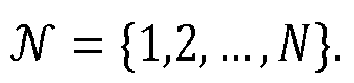
- the goal is to train the learnable parameters 0 of the CNN to rank, for each given query image I q , its similarity to every image from a database ⁇ I i ⁇ 1 ⁇ i ⁇ N of size N.
- Database images are then sorted according to their similarities in decreasing order.
- R N ⁇ N ⁇ N denote the ranking function, where R ( S q ,i ) is the index of the i -th highest value of S q .
- R ( S q ) denotes the ranked list of indexes for the database.
- the quality of the ranking R ( S q ) can then be evaluated with respect to the ground-truth image relevance, which is the above mentioned known similarity between each pair of images of the training set, denoted by the binary ground-truth labels Y q in ⁇ 0,1 ⁇ N , where Y i q is 1 if I i is similar (or "relevant") to I q and 0 otherwise.
- IR metrics such as average precision (AP), F-score, and discounted cumulative gain.
- AP average precision
- F-score F-score
- discounted cumulative gain IR metrics are used to assess how well the search results satisfy the user's query intent. This is rendered possible through the fact that the images of the batch used during the training phase are known and that their respective similarities are known through the above mentioned ground-truth labels.
- One of the IR metrics is the fraction of the images retrieved that are relevant to the user's information need.
- AP is a good metric for IR when the ground-truth labels are binary, as is the case for Y i q as defined above.
- AP does not depend on a threshold, rank position or number of relevant (or similar) images, and is thus simpler to employ and better at generalizing for different queries.
- the learnable parameters of f ⁇ should be trained using stochastic optimization such that they maximize AP on the training set. This is not feasible for the original AP formulation, because of the presence of the indicator function 1[ ⁇ ].
- a listwise ranking loss function developed for histograms is used to overcome this issue.
- the key is to perform the training of the CNN with a relaxation of the AP, obtained by replacing the indicator function by a function ⁇ , whose derivative can be back-propagated to adapt the learnable parameters of the CNN, where ⁇ soft-assigns similarity values into a fixed number of bins.
- This approach is called "histogram binning".
- precision and incremental recall are calculated at every rank k in ⁇ 1, ..., N ⁇ .
- the second step is to use a soft assignment as replacement of the indicator function. This is achieved by using the function ⁇ : R ⁇ 1 , 2 , ... , M ⁇ 0 1 such that each ⁇ ( ⁇ , m ) is a triangular kernel centered around b m and width 2 ⁇ , i.e.
- ⁇ x m max 1 ⁇ x ⁇ b m ⁇ , 0
- ⁇ ( x , m ) is a soft binning of x that approaches the indicator function 1[ x ⁇ b m ] when M ⁇ ⁇ while being differentiable with respect to x :
- ⁇ ⁇ x m ⁇ x ⁇ sign x ⁇ b m ⁇ 1 x ⁇ b m ⁇ ⁇
- ⁇ ( S q , m ) is a vector in [0,1] N that indicates the soft assignment of S q to the bin b m .
- Fig. 2 shows a scatter plot of AP versus AP Q for all queries of the Paris dataset, on which a correlation of circa 0.98 between them is visible.
- the chain rule ensures that each gradient (i.e., partial derivative) of the loss function with respect to one of the learnable parameters of the CNN (which have to be back-propagated to the respective learnable parameters of the CNN to train the CNN) can be decomposed into a sum of sub-gradients, each sub-gradient being computed with respect to a single image of the batch.
- an algorithm exploiting this chain rule is provided, that solves this memory issue and allows the training of a network of arbitrary depth, with arbitrary image resolution and batch size, without approximating the loss function defined above.
- the algorithm consisting of three stages, is illustrated in Fig. 3 and detailed below.
- the global feature descriptors of all training images of a batch of images are computed, but the intermediary tensors obtained during the computation (i.e. the tensors obtained at each internal node of the CNN) are discarded.
- the intermediary tensors are not needed and can be discarded. Since all tensors considered are compact (i.e. the global feature descriptors and the score matrix), this operation consumes little memory.
- the global feature descriptors are recomputed, this time storing the intermediary tensors.
- This operation occupies a lot of memory, but it can now be performed image by image.
- the back-propagation through the network can now be performed.
- each gradient with respect to a given learnable parameter is accumulated, one image at a time, before finally updating the network learnable parameters with the help of the corresponding gradients, as shown in the last step of the algorithm below.
- This updating step corresponds to the above mentioned back-propagation, through which the learnable parameters of the CNN are iteratively adapted until the loss function converges towards a minimum and the training phase is concluded.
- the original Landmarks dataset contains 213,678 images divided into 672 classes. However, since this dataset has been created semi-automatically by querying a search engine, it contains a large number of mislabeled images. An automatic cleaning process can be performed to clean this dataset, and the result is called the L andmarks-clean dataset. It contains 42,410 images and 586 landmarks, and it is the version used to train the CNN in all the experiments discussed below.
- the Revisited Oxford ( Oxford) and Revisited Paris ( Paris) datasets contain 4,993 and 6,322 images respectively, with 70 additional images for each that are used as queries (see Fig. 4 for example queries). These images are further labeled according to the difficulty in identifying which landmark they depict (Easy, Hard, Unclear, and Negative). These categories are then used to determine three evaluation protocols for these datasets:
- a set of 1 million distractor images can be added to each dataset to make the task more realistic. Since these new datasets are essentially updated versions of the original Oxford and Paris datasets, with the same characteristics but more reliable ground-truth labels, these revisited versions have been used in the experiments discussed below.
- ResNet-101 is a specific instantiation of a CNN architecture making use of 101 convolution layers, from the paper " Deep residual learning for image recognition" by K. He, X. Zhang, S. Ren, and J. Sun, in Conference on Computer Vision and Pattern Recognition, CVPR, 2016 . Further, the original final layer of the ResNet-101 CNN (which was specific to a classification algorithm) has been replaced by a generalized-mean pooling (GeM) layer.
- GeM generalized-mean pooling
- the GeM layer is a particular type of layer which performs global feature pooling (i.e. it transforms an image of variable width and height into a fixed size vector).
- the GeM layer contains a single trainable parameter which is trained through back-propagation of the gradients, as the rest of the network parameters.
- the above REsNet-101 network is trained according to the Adam optimizer of D.P. Kingma and J. Ba: "Adam: a method for stochastic optimization", arXiv preprint, 2014 .
- the weight decay (which specifies how the learnable parameters are updated during back-propagation) is set to 10 -6
- the set of training images is augmented by generating additional training images through standard data augmentation (by applying e.g., color jittering, random scaling, rotation and cropping).
- color jittering random scaling, rotation and cropping
- Training images are cropped to a fixed size of 800 ⁇ 800, but during test, the original images (unscaled and undistorted) are fed into the CNN.
- the AP Q loss function depends on the number of quantization bins M in Eq. 7.
- M 20 quantization bins have been used in all other experiments.
- Each batch is constructed by sampling random images from each dataset class (all classes are hence represented in a single batch). Experiments showed that sampling the classes did not lead to any difference, as illustrated by Fig. 7 . Due to the dataset imbalance, certain classes are constantly over-represented at the batch level. To counter-balance this situation, a weight has been introduced in Eq. 12 to weight equally all classes inside a batch. Two CNNs have been trained with and without this weighting. The results are presented in Fig. 8 . The improvement in terms of mean average precision with class weighting is around +2% and shows the importance of this balancing.
- a bias can occur in the ranking of the images according to their similarities if "ties" are present in the embedding space.
- ties relate to images having global feature descriptors in the embedding space that are at the same distance to the query image and therefore equally similar to the query image. In such a case, an uncertainty occurs regarding how these images should be ranked in the final result.
- AP T a tie-aware version of the AP Q loss function
- a simplified tie-aware AP loss function has also been used and its efficiency has been compared to the one of AP Q .
- Fig. 9 The absolute difference in terms of mean average precision is presented in Fig. 9 , which shows that the mAP Q loss function, straightforwardly derived from the definition of AP, consistently outperforms the tie-aware formulation by a small but significant margin. This may be due to the fact that the tie-aware formulation used in practical implementations is in fact an approximation of the theoretical tie-aware AP. Accordingly, the mAP Q loss function has been used in all subsequent experiments.
- Descriptor whitening is frequently used in the art to improve the performance of global feature descriptors. It consists in multiplying a global feature descriptor (extracted e.g. from the Landmarks dataset described above) by a matrix obtained using principal component analysis (PCA) on the image representations of the training set.
- PCA principal component analysis
- a PCA returns the eigenvalues (Dx1 vector) and the eigenvectors (DxD matrix).
- a PCA matrix M diagonal(sqrt(eigenvalues)) * eigenvectors, where diagonal() creates a diagonal matrix from a vector and sqrt() computes the element-wise square-root.
- the global feature descriptors are then normalized at test time using the computed PCA. The above defined square-rooted PCA was found to be more effective. Whitening has been used in all subsequent experiments.
- a deep feedforward network (DFN) or a convolutional forward network (CFN) can be used.
- DNN deep feedforward network
- CNN convolutional forward network
- Fig. 10 is a functional block diagram illustrating a computer-implemented method for training a CNN according to an embodiment. It begins at step 1002 , at which a batch (or a set) of training images is obtained. Obtaining the training images encompasses that they can be received from a user dealing with the training phase of the CNN or from any memory location (e.g. a local or remote computing system, a local or remote database, a cloud storage or any other memory location known in the field) on which they are stored. Alternatively, the images of the batch can be retrieved by a user or automatically retrieved from any of these memory locations. The images of the batch used for the training phase are known, and in particular their respective similarities are known, thereby providing the ground-truth image relevance mentioned above.
- a batch or a set
- Obtaining the training images encompasses that they can be received from a user dealing with the training phase of the CNN or from any memory location (e.g. a local or remote computing system, a local or remote database, a cloud storage
- the ground-truth image relevance consists for example in a set of known binary ground-truth labels (one label for each pair of images of the batch), each label of a given pair of images informing whether these images are similar (in which case, the label is equal to 1) or not (in which case, the label is equal to 0).
- the received batch can be one of the datasets of known images mentioned above, i.e. Paris or Oxford.
- the training images of the batch are high-resolution images of more than 1 Megapixels.
- a global feature descriptor is computed in an embedding space for each image of the received batch. This is achieved by inputting each image of the batch into the CNN to be trained and getting the corresponding global feature descriptor as output of the CNN.
- the global feature descriptors are vectors defined in a multi-dimensional space called the embedding space, and each global feature descriptor describes uniquely the corresponding image in the embedding space.
- the CNN can be a ResNet CNN, for example a ResNet-101, which has 101 convolution layers. However, any number of layers higher than 20 layers, and preferably around 100 layers, may be used as well.
- the original CNN i.e., the CNN with the original values of its learnable parameters before the training phase begins
- any available CNN that has been trained for classification tasks can also be used as original CNN.
- a similarity is computed between each given pair of images of the batch based on a distance between the global feature descriptors in the embedding space.
- Any known distance metric can be used to compute these similarities.
- an Euclidean metric can be used to determine the distance between two global feature descriptors in the embedding space, and the similarity between two images can be a value proportional to the Euclidean distance between the corresponding global feature descriptors.
- any other definition of the similarity can be used, based on any definition of the distance between global feature descriptors in the embedding space, without departing from the scope of the embodiments disclosed herein.
- a ranking function R is applied to the images of the batch to sort them based on their similarities. For example, each image of the batch is considered to be an initial query image, and the remaining images of the batch are ranked (or sorted) according to their similarities to the query image.
- the images of the batch can be ranked by decreasing or by increasing similarity.
- An example of the ranking obtained in this step for a given query image can be found in Fig. 4 discussed above, at different training stages of the CNN (i.e., at different numbers of iterations of the training method illustrated in Fig. 10 ).
- the quality of the obtained rankings is evaluated according to an average precision (AP) ranking evaluation metric.
- AP average precision
- evaluating the quality of a ranking is performed by computing an average precision of the ranking compared to the known relative similarities between the images of the batch.
- the AP is the sum over all images of the product of a precision at rank k times an incremental recall from ranks k-1 to k, where the precision at rank k is the proportion of relevant images found in the k first indexes of the ranking, and the incremental recall is the proportion of relevant images found at rank k out of a total of relevant images.
- the AP is reformulated into a differentiable AP called quantized AP (or AP Q ) using histogram binning and quantization.
- Reformulating the AP ranking evaluation metric into AP Q comprises replacing the indicator function in the AP ranking evaluation metric by a quantization function ⁇ being a set of triangular kernels each centered around a bin center b m of an histogram binning. For details on this step, it is referred to the section "Quantization function" above.
- step 1014 the mean of AP Q (mAP Q ) over the batch of training images is computed.
- mAP Q mean of AP Q
- Training procedure the section "Training procedure” above.
- the listwise ranking loss function L(D,Y) as defined above in Eq. 13 is computed based on mAP Q .
- the listwise ranking loss function is a loss function adapted to optimize ranking during the training phase of the CNN, which takes a variable number of training images at the same time and optimizes their ranking jointly, wherein the listwise ranking loss function is minimal when the variable number of training images has been ranked correctly by the ranking function during the training phase.
- each given learnable parameter of the CNN is adapted through back-propagation of the gradient of mAP Q with respect to the given learnable parameter.
- step 1018 it is determined whether the listwise ranking loss function based on mAP Q has converged towards a minimum (or equivalently whether mAP Q converges towards a maximum), meaning that the ranking function optimally ranks the training images and obtains a result similar to the expected result (complying with the known ground-truth image relevance). For example, this determination can be performed by comparing the newly computed value of mAP Q in step 1014 with the previous value of mAP Q (or the respective new and previous values of the corresponding loss function) and determining whether these values are equal or at least whether the difference between the new value and the previous value falls below a predetermined threshold.
- any other method for determining convergence can be used without departing from the scope of the present disclosure.
- the method ends at step 1020 at which the training phase is concluded.
- the trained CNN can then be applied to image retrieval with any set of images, as will be described in detail in relation with Fig. 11 .
- the training steps 1004 to 1016 are repeated until convergence is achieved.
- determining step 1016 could also be performed immediately after step 1014 and a last adaptation of the learnable parameters could thereby be avoided in case convergence is achieved, since this last adaptation will not modify (or at least not substantially modify) the learnable parameters once convergence has been achieved.
- Fig. 11 is a functional block diagram illustrating a method for image retrieval in response to the reception of a query image according to an embodiment.
- This method can be performed by applying the trained CNN (obtained at the end of the method of Fig. 10 ,) to an unknown set of images distinct from the training batch of images as soon as the training phase illustrated in step 1020 of Fig. 10 has been concluded, i.e. as soon as mAP Q has converged, which means that the learnable parameters of the CNN have been learned successfully and that the CNN is now ready for general image retrieval tasks.
- the steps performed for responding to a query image are at least in part similar to the steps performed during the training phase described in relation with Fig. 10 , but without having to evaluate the ranking function anymore, nor having to adapt the learnable parameters of the CNN.
- the measure of similarities between the images based on the distances between their corresponding global feature descriptors in the embedding space is now optimal.
- the function defining the global feature descriptor of an image, as encoded within the CNN is now optimal for comparing input images and ranking them according to a similarity measure.
- a (potentially unknown) query image is obtained.
- Obtaining the query image encompasses as well embodiments in which the query image is received as embodiments in which the query image is retrieved.
- This query image may be received from a user or from any other source, manually or automatically. Alternatively, it may be retrieved by the user or automatically by programming means like e.g. an application.
- the source may be local or remote, and may be e.g. a database or any type of digital memory or any source from which an image can be digitalized. Alternatively, the source itself may be an application or any type of program code having access to images stored in memory.
- the query image may pertain to the batch of training images, but may be as well any new image that has never been input into the CNN before.
- the query image may be a high-resolution image of at least 65000 pixels.
- the query image is input into the CNN which has been previously trained (e.g. according to the method of Fig. 10 ), and a corresponding global feature descriptor is output by the trained CNN.
- the learnable parameters of the CNN have been learned by training the CNN on a known batch of training images using a listwise ranking loss function directly optimizing a quantized mean average precision, mAP Q , ranking evaluation metric.
- a similarity is measured between the query image and each other image previously input into the CNN, based on a distance in the embedding space between the global feature descriptor of the query image and the respective global feature descriptors of the other images.
- the images that have been previously input into the CNN are ranked based on their similarity to the query image, for example ranked by decreasing similarity.
- a set of images is selected based on the similarity of the images of the set to the query image and a set of identifiers representative of the set of images is output.
- the set of identifiers may identify the images themselves or other data associated with the images such as a class (for image categorization), an object such as a person's name (for facial/retinal recognition), or a location (from location data associated with metadata of images) etc.
- these identifiers and/or the selected set of images itself may then be provided to the user or to any other target person or target location in response to his/her query.
- all the images previously input into the CNN can be provided.
- only a predetermined number of the most similar images could be provided.
- the images can be ranked by decreasing similarity.
- embodiments are also contemplated where the resulting set of images provided to the user is not ranked, or ranked by increasing similarity, or according to any other criterion independent of the similarity.
- Fig. 12 is a functional block diagram illustrating a method for optimizing one iteration of the training of the CNN over a large number of input images according to an embodiment. It corresponds to the algorithm described above in the section "Training for high-resolution images" that can be applied to implement steps 1004 to 1016 of the training phase of the CNN described above in relation with Fig. 10 , for adapting the learnable parameters of the CNN.
- This three-stage algorithm is optimized to spare memory and time, since in view of the fact that the CNN is trained with high-resolution images of arbitrary high size and resolution, computing the gradients of the loss function with respect to all the learnable parameters of the CNN over all the images of the training batch would be infeasible in practice.
- the overall idea behind this algorithm is to use the chain rule in the computation of the gradients (in the second stage of the algorithm) in order to compute the gradients recurrently by successively adding the contribution of each given image to the gradients, one image at a time, thereby freeing the memory of the computations made for one image before treating the contribution of the next image to the gradients.
- step 1202 it begins with a first stage at step 1202 , at which the global feature descriptors of all the images of the training batch are computed, but where all the intermediary tensors obtained during the computation are discarded.
- a second stage at step 1204 the similarities between each pair of images in the batch are computed, as well as the listwise ranking loss function (or, equivalently, mAP Q ), and the gradients of the loss function (or, equivalently, of mAP Q ) with respect to the global feature descriptors of the images of the batch.
- the listwise ranking loss function or, equivalently, mAP Q
- the gradients of the loss function or, equivalently, of mAP Q
- a loop is initiated over the images in the batch (through the determination, at step 1212 , whether there are still one or more images in the batch that have not been treated yet), and for each given image of the batch (selected in step 1206 ), the following steps are performed: first, at step 1208 , its global feature descriptor is recomputed, the gradients of the loss function (or, equivalently, of mAP Q ) with respect to the learnable parameters of the CNN are computed, and this time the intermediary tensors obtained during the computation are kept in memory; secondly, at step 1210 , for each learnable parameter of the CNN, a gradient is computed as follows: after an initialization of all gradients to zero before the first image is treated in this third stage, the contribution of the given image to this gradient is added to the previous value of this gradient. Once all the images of the batch have been treated one by one, the final gradients with respect to each learnable parameter have been fully computed and they can be back-propagated at
- mAP Q is the mean over the batch of training images of a quantized average precision ranking evaluation metric, AP Q , which is a quantized version of an average precision, AP, ranking evaluation metric that has been rendered differentiable using histogram binning and quantization.
- the intermediary tensors of the last image that has been treated can be kept in memory and this image can be the first one to be selected in step 1206, in order to avoid an unnecessary re-computation of the global feature descriptor of the last image.
- Fig. 12 the order and the number of the steps of Fig. 12 are illustrative. They are not meant to be restrictive and all the alternative embodiments that a skilled person would consider in order to implement the same general idea are also contemplated without departing from the scope of the present disclosure.
- the loop performed on the images of the batch can be implemented according to any alternative formulation that would fall within the usual skills of a person skilled in the art.
- Table 1 summarizes the performance of the best-performing methods on the datasets listed in section 5.1 without query or database expansion.
- the notation of (Radenovic et al. 2018) is used as this helps to clarify important aspects about each method. Namely, generalized-mean pooling (Radenovic, Tolias, and Chum 2018) is denoted by GeM and the R-MAC pooling (Tolias, Sicre, and Jegou 2016) is denoted by R-MAC.
- CL contrastive loss
- TL triplet loss
- AP AP Q loss described above
- O if no loss is used (i.e. off-the-shelf features).
- embodiments according to the described model outperform the state of the art by 1% to 5% on all datasets and protocols.
- the described model is more than 4 points ahead of the best reported results (Radenovic, Tolias, and Chum 2018) on the hard protocol of Oxford and Paris.
- This is remarkable since the described model uses a single scale at test time (i.e. the original test images), whereas other methods boost their performance by pooling feature descriptors computed at several scales.
- the trained CNN described above does not undergo any special pre-training step (it has been initialized with ImageNet-trained weights), again unlike most competitors from the state of the art. Empirically one observes that the AP Q loss renders such pre-training stages obsolete.
- the training time is also considerably reduced: training the described CNN from scratch takes a few hours on a single P40 GPU.
- results with query expansion (QE) and database augmentation (DBA) are reported at the bottom of Table 1 .
- the described model with QE outperforms other methods also using QE in 6 protocols out of 8.
- Some or all of the method steps may be implemented by a computer in that they are executed by (or using) a processor, a microprocessor, an electronic circuit or processing circuitry.
- the embodiments described above may be implemented in hardware or in software.
- the implementation can be performed using a non-transitory storage medium such as a computer-readable storage medium, for example a floppy disc, a DVD, a Blu-Ray, a CD, a ROM, a PROM, and EPROM, an EEPROM or a FLASH memory.
- a computer-readable storage medium for example a floppy disc, a DVD, a Blu-Ray, a CD, a ROM, a PROM, and EPROM, an EEPROM or a FLASH memory.
- Such computer-readable media can be any available media that can be accessed by a general-purpose or special-purpose computer system.
- embodiments can be implemented as a computer program product with a program code or computer-executable instructions, the program code or computer-executable instructions being operative for performing one of the methods when the computer program product runs on a computer.
- the program code or the computer-executable instructions may, for example, be stored on a computer-readable storage medium.
- a storage medium (or a data carrier, or a computer-readable medium) comprises, stored thereon, the computer program or the computer-executable instructions for performing one of the methods described herein when it is performed by a processor.
- an apparatus comprises one or more processors and the storage medium mentioned above.
- an apparatus comprises means, for example processing circuitry like e.g. a processor communicating with a memory, the means being configured to, or adapted to, perform one of the methods described herein.
- processing circuitry like e.g. a processor communicating with a memory, the means being configured to, or adapted to, perform one of the methods described herein.
- a further embodiment comprises a computer having installed thereon the computer program or instructions for performing one of the methods described herein.
- Fig. 13 which comprises server 100 and one or more client devices 102 that communicate over a network 104 (which may be wireless and/or wired) such as the Internet for data exchange.
- Server 100 and the client devices 102 include a data processor 112 and memory 113 such as a hard disk.
- the client devices 102 may be any device that communicates with server 100, including autonomous vehicle 102b, robot 102c, computer 102d, or cell phone 102e.
- the query image obtained in step 1102 of the method of performing image retrieval corresponds to a query initiated by client device 102.
- the query is processed at server 100, which returns processed identifiers representative of the set of images to client device 102.
- the query can be processed at the client device 102 that initiated the query.
- the method for training learnable parameters of a CNN may also be performed at server 100 or in an alternate embodiment at a different server or in another alternate embodiment at the client device 102.
Landscapes
- Engineering & Computer Science (AREA)
- Physics & Mathematics (AREA)
- Theoretical Computer Science (AREA)
- General Physics & Mathematics (AREA)
- Data Mining & Analysis (AREA)
- General Engineering & Computer Science (AREA)
- Mathematical Physics (AREA)
- Software Systems (AREA)
- Life Sciences & Earth Sciences (AREA)
- Computing Systems (AREA)
- Computational Linguistics (AREA)
- Evolutionary Computation (AREA)
- Artificial Intelligence (AREA)
- Databases & Information Systems (AREA)
- Molecular Biology (AREA)
- Biophysics (AREA)
- Biomedical Technology (AREA)
- Health & Medical Sciences (AREA)
- General Health & Medical Sciences (AREA)
- Mathematical Optimization (AREA)
- Computational Mathematics (AREA)
- Mathematical Analysis (AREA)
- Pure & Applied Mathematics (AREA)
- Algebra (AREA)
- Bioinformatics & Computational Biology (AREA)
- Evolutionary Biology (AREA)
- Bioinformatics & Cheminformatics (AREA)
- Probability & Statistics with Applications (AREA)
- Operations Research (AREA)
- Computer Vision & Pattern Recognition (AREA)
- Image Analysis (AREA)
- Information Retrieval, Db Structures And Fs Structures Therefor (AREA)
Abstract
Description
- The present disclosure relates to image retrieval and, in particular, to a system, method and computer-readable medium for performing image retrieval using a convolutional neural network (CNN).
- Image retrieval consists in finding, given a "query image", all images containing relevant content within a large database. Relevance here is defined at the image level and retrieval typically consists in ranking in top positions database images with the same object instance as the one in the query image. This important technology serves as a building block for popular applications such as image-based item identification (e.g., fashion items or products) and automatic organization of personal photos.
- Most image retrieval approaches rely on computing image signatures (also called "global feature descriptors" in this disclosure) that are robust to viewpoint variations and other types of noise. Interestingly, descriptors extracted by deep learned models using trained convolutional neural networks (CNNs) have recently outperformed traditional keypoint-based methods. This good performance was enabled by the ability of deep learned models to leverage a family of loss functions well-suited to the ranking problem.
- Early works on image retrieval relied on local patch descriptors (e.g. descriptors obtained through the scale-invariant feature transform, also called SIFT descriptors), aggregated using bag-of-words representations or more elaborate schemes to produce a global feature descriptor for each image, that could then be compared to one another in order to find their closest matches. Recently, global feature descriptors directly extracted with CNNs have emerged as an alternative. While initial work used neuron activations extracted from off-the-shelf networks pre-trained for classification, it was later shown that networks could be trained specifically for the task of image retrieval in an end-to-end manner using a siamese network (which is an artificial neural network that uses the same weights while working in tandem on two different input vectors to compute comparable output vectors). The key was to leverage a loss function that optimizes ranking instead of classification. This class of approaches represents the current state of the art in image retrieval with global representations.
- In the more restrictive context of patch retrieval (where a patch is a small square of up to 100 * 100 pixels with limited visual content within an image and is therefore orders of magnitude smaller than the image in which it is embedded), He et al. (K. He, Y. Lu, and S. Sclaroff: "Local descriptors optimized for average precision", in Conference on Computer Vision and Pattern Recognition, CVPR, 2018) have shown that when training a network for outputting a local feature descriptor for each patch within an image, the mean average precision (mAP) metric can be optimized directly. While the average precision (AP) is a non-smooth and non-differentiable function, He et al. have shown that it can be approximated based on the differentiable approximation to histogram binning proposed by Ustinova et al. (E. Ustinova and V. Lempitsky: "Learning deep embeddings with histogram loss", in Neural Information Processing Systems, NIPS 2016). This approach radically differs from those based on local loss functions. The use of histogram approximations to mAP is called listwise, as the loss function takes a variable (possibly large) number of examples at the same time and optimizes their ranking jointly.
- Apart from He et al., several relaxations or alternative formulations have been proposed in the literature to allow for the direct optimization of the AP loss function (A. Behl et al.: "Optimizing average precision using weakly supervised data", Institute of Electrical and Electronics Engineers, IEEE TPAMI 2015; T. Hazan et al.: "Direct loss minimization for structure prediction", in NIPS 2010; P. Henderson and V. Ferrari: "End-to-end training of object class detectors for mean average precision", in Asian Conference on Computer Vision, ACCV 2016; P. Mohapatra et al: "Efficient optimization for average precision SVM", in Neural Information Processing Systems, NIPS 2014; Y. Song et al.: "Training deep neural networks via direct loss minimization", in International Conference on Machine Learning, ICML 2016; Y. Yue et al.: "A support vector method for optimizing average precision", in Special Interest Group on Information Retrieval, SIGIR 2007). For example, Yue et al. proposed to optimize the AP through a loss-augmented inference problem under a structured learning framework using linear support vector machines (SVMs). Song et al. then expanded this framework to work with non-linear models. However, both works assume that the inference problem in the loss-augmented inference in the structured SVM formulation can be solved efficiently. Moreover, their technique requires using a dynamic-programming approach which requires changes to the optimization algorithm itself, complicating its general use. A loss function based on average precision had not been implemented for the general case of CNNs trained with arbitrary learning algorithms until He et al. and Henderson and Ferrari. Henderson and Ferrari focused on object detection, while He et al. focused on patch verification, retrieval, and image matching based on a set of local feature descriptors obtained for the patches.
- However, a new approach is still needed in the context of image retrieval, where additional hurdles must be cleared because, in particular, the images are orders of magnitude bigger than the patches.
- In order to overcome the above deficiencies, an approach to image retrieval is presented here that makes use of a listwise ranking loss function directly optimizing the mean average precision metric (abbreviated into mAP metric or simply mAP in the following disclosure) and outperforms prior art approaches. Further, the approach presented in this disclosure relies on a multi-stage optimization scheme that makes training feasible on existing GPUs for arbitrary batch sizes, image resolutions and network depths.
- In more detail, for achieving these goals during the training phase of a convolutional neural network (CNN), the mAP metric is optimized directly to improve the ranking of images according to their similarity to a query image. For this purpose, the global feature descriptor of an input image is obtained directly as output of the CNN in response to the input image being fed into the CNN. The multi-dimensional space in which the global feature descriptors are defined is called the embedding space, and the similarity between two images is computed on the basis of a distance between their global feature descriptors in the embedding space. As the AP loss function directly optimizes (a close approximation to) the mAP which is measured when evaluating an image retrieval system, it does not suffer from the aforementioned drawbacks: as will be shown, there is no need for pre-training or hard-negative mining, and the convergence is much faster.
- In an embodiment, a computer-implemented method of performing image retrieval is provided. The method comprises the steps of: obtaining a query image; computing a global feature descriptor of the query image by inputting the query image into a trained CNN and obtaining the global feature descriptor in an embedding space as output, wherein learnable parameters of the convolutional neural network have been learned by training the CNN on a known batch of training images using a listwise ranking loss function directly optimizing a mean average precision ranking evaluation metric; computing a similarity between the query image and images that have been previously input into the CNN based on a distance in the embedding space between the global feature descriptor of the query image and the global feature descriptors of the images that have been previously input into the CNN; applying a ranking function to the images that have been previously input into the CNN to obtain a ranking of these images based on their similarity to the query image; selecting a set of images based on their similarity to the query image; and outputting a set of identifiers representative of the set of images.
- In another embodiment, a computer-implemented method is provided for training learnable parameters of a CNN on a known batch of training images in a memory-efficient way through a three-stage algorithm. The method comprises the steps of: computing a global feature descriptor for each image of the batch in the embedding space, but discarding intermediary tensors obtained during the computation of the global feature descriptor in the memory; computing a similarity between each pair of images in the batch, a listwise ranking loss function, and gradients of the loss function with respect to the global feature descriptors, without performing back-propagation of the gradients to the learnable parameters at that time; processing all the images of the batch by: selecting a given image of the batch, re-computing the corresponding global feature descriptor of the given image and the gradients of the loss function with respect to the learnable parameters of the CNN, and keeping the intermediary tensors in the memory, adding, for each given learnable parameter of the CNN, the contribution of the given image to an overall gradient of the loss function with respect to the given learnable parameter, and repeating the processing steps until it is determined that there is no remaining unselected image in the batch. Once it is determined that there is no remaining unselected image in the batch, back-propagating each overall gradient of the loss function to adapt the corresponding learnable parameter of the CNN, and repeating all steps of the method until it is determined that the listwise ranking loss function has reached a minimum.
- According to a further embodiment, one or more computer-readable media storing thereon computer-executable instructions are provided. When carried out by a processor, the computer-executable instructions cause the processor to perform the computer-implemented method of performing image retrieval described above.
- According to a further embodiment, one or more other computer-readable media storing thereon computer-executable instructions are provided. When carried out by a processor, the computer-executable instructions cause the processor to perform the computer-implemented method described above for training learnable parameters of a CNN on a known batch of training images in a memory-efficient way through a three-stage algorithm.
- According to a further embodiment, an apparatus comprising processing circuitry is provided, wherein the processing circuitry is configured to perform the computer-implemented method of performing image retrieval described above.
- According to a further embodiment, an apparatus comprising processing circuitry is provided, wherein the processing circuitry is configured to perform the computer-implemented method described above for training learnable parameters of a CNN on a known batch of training images in a memory-efficient way through a three-stage algorithm.
- The accompanying drawings are incorporated into and form a part of the specification for the purpose of explaining the principles of the embodiments. The drawings are not to be construed as limiting the embodiments to only the illustrated and described embodiments of how they can be made and used. Further features and advantages will become apparent from the following and more particularly from the description of the embodiments, as illustrated in the accompanying drawings, wherein:
-
Figure 1 illustrates the differences between using a local ranking loss function calculated based on an input of a triplet of images into the CNN (on the left side of the figure) versus using a listwise ranking loss function calculated based on an input of a large number of images into the CNN for training the CNN according to an embodiment (on the right side of the figure); -
Figure 2 is a scatter plot of the average precision (AP) versus the quantized version of the AP (APQ) used in an embodiment for a known set of images calledParis;
-
Figure 3 illustrates an optimized algorithm for training the CNN over a large number of input images according to an embodiment; -
Figure 4 illustrates the evolution of a training process over time through examples of answers to an image query obtained with the trained CNN with the known set of imagesOxford after three given numbers of iterations (8, 48 and 152 iterations);
-
Figure 5 is a plot of mAPQ as a function of the number of quantization bins; -
Figure 6 is a plot of mAPQ as a function of the batch size; -
Figure 7 is a plot of mAPQ as a function of the number of sampled classes per batch; -
Figure 8 is a histogram showing the improvement in terms of mAPQ obtained for four distinct batches of known images by balancing the AP weights when computing the AP loss function such that all classes are weighted equally within a batch, according to an embodiment; -
Figure 9 is a histogram showing the improvement in terms of mAP obtained for four distinct batches of known images when APQ is used, according to an embodiment, when compared to a tie-aware version of AP called APT; -
Figure 10 is a functional block diagram illustrating a method for training the CNN according to an embodiment; -
Figure 11 is a functional block diagram illustrating a method for image retrieval in response to the reception of a query image according to an embodiment; -
Figure 12 is a functional block diagram illustrating a method for optimizing the training of the CNN over a large number of input images according to an embodiment; and -
Figure 13 illustrates an example of architecture in which the disclosed methods may be performed. - Described herein are systems and methods for image retrieval. For purposes of explanation, numerous examples and specific details are set forth in order to provide a thorough understanding of the described embodiments. Embodiments as defined by the claims may include some or all of the features in these examples alone or in combination with other features described below, and may further include modifications and equivalents of the features and concepts described herein. The illustrative embodiments will be described with reference to the drawings wherein like elements and structures are indicated by like reference numbers.
- Image retrieval can be seen as a "learning to rank" problem. In this framework, the task is to determine in which order elements from the training set should appear. It is solved using metric learning combined with an appropriate ranking loss function. In machine learning, a loss function (also called "cost function", or simply "loss") is a function that maps an event or values of one or more variables onto a real number representing some "cost" associated with the event.
- In order to obtain a CNN able to rank images according to their similarity, which can then be used for image retrieval, the CNN must first be "trained". The "training phase" of the CNN aims at optimizing internal, learnable parameters of the CNN by training it on a set of images for which the expected result is known (i.e., in the present case, the similarity between each pair of images of the set is known in terms of binary ground-truth labels for each pair of images, as explained in more detail below). For this purpose, each image of the training set is input in the CNN, which outputs a vector value called a global feature descriptor of the image within a multi-dimensional space (also called the "embedding space"). A distance can be defined between any pair of global feature descriptors in the embedding space, according to any suitable distance metric (like e.g. the Euclidean distance metric). Based on this distance, it becomes possible to define a similarity between pairs of images, where the similarity between two images decreases when the distance between them increases. If an image of the set is chosen as starting point (corresponding to the "query image" for which a user may want to find similar images using the CNN once it will have been trained), all the images of the training set can then be ranked in terms of decreasing similarity with respect to the chosen image. An adequately chosen loss function can then be applied to the ranking for evaluating the efficiency (or degree of validity) of this ranking, based on the known similarities between each pair of images. The better the ranking obtained by the CNN is, the smaller will be the result of the loss function.
- The aim of the training phase is to modify the internal, learnable parameters of the CNN so that they minimize the result of the loss function. This optimization of the loss function (which must be convergent towards a minimum) is rendered possible by the back-propagation of so called "loss gradients", which are obtained from the partial derivatives of the loss function with respect to the learnable parameters of the CNN. These loss gradients are "back-propagated" to the respective learnable parameters in that they are used to modify (or adapt or update) the learnable parameters to perform better at the next iteration of the training phase. Indeed, at the next iteration, the CNN will output global feature descriptors of the images computed with the help of the modified learnable parameters, and these global feature descriptors will be better suited for ranking the images, leading to a better evaluation of the ranking obtained by the CNN (i.e. to a lower value of the loss function) and to a smaller adaptation of the learnable parameters at the next back-propagation of the loss gradients, until the loss function converges towards a minimum and no adaptation of the learnable parameters is necessary anymore. Once the loss function has converged, the CNN has been successfully trained, and it can then be used to perform image retrieval.
- According to an embodiment, performing image retrieval includes receiving a query image, computing its global feature descriptor, computing the similarities between the query image and any other image for which a global feature descriptor has already been obtained (using the chosen distance metric in the embedding space mentioned above), and then ranking the images in decreasing order of similarity with respect to the query image.
- Most works in image retrieval have considered pairwise or tuplewise (e.g., triplet-based, n-tuple-based) ranking loss functions, which are called here local loss functions because they act on a fixed and limited number of examples before computing the gradient. Their common principle is to subsample a small set of images, verify that they locally comply with the ranking objective, perform a small model update of the learnable parameters if they do not, and repeat these steps until convergence. In other words, for such loss functions, training consists in repeatedly sampling random and difficult pairs or triplets of images, computing the loss function, and back-propagating its gradients.
- Compared to classification losses previously used for retrieval with less success, ranking-based loss functions directly optimize for the end task, enforcing intra-class discrimination and more fine-grained image representations. However, despite their effectiveness, properly optimizing a local loss can be a challenging task, for several reasons, and important problems remain. First, it is not clear from a theoretical standpoint if the quantity that these approaches are minimizing, termed the essential loss, is well aligned with standard evaluation metrics such as mean average precision (mAP). Second, the total number of possible pairs or triplets, for instance, is increasing quadratically or cubically with the size of the datasets, but only an unknown fraction of them is in fact useful to the optimization. This total number largely exceeds in practice the allowable training time, thereby preventing to fully exploit the available information during training. For these reasons, many complicated steps are required to obtain good results, e.g., pre-training for classification, combining multiple losses, and using complex hard-negative mining strategies (i.e. biasing the sampling of image pairs by mining hard or semi-hard negative examples). These engineering heuristics are complicated to implement and tune. Besides being less than straightforward, mining hard examples is often time consuming. Another major problem is the fact that local loss functions only optimize an upper bound on the true ranking loss. As such, there is no theoretical guarantee that the minimum of the loss actually corresponds to the minimum of the true ranking loss.
- In this disclosure, a new type of ranking loss function called listwise ranking loss function that directly optimizes mAP is described, as illustrated in
Fig. 1 . As mentioned above, listwise loss functions allow to reformulate AP using histogram binning. AP is normally non-smooth and not differentiable, and cannot be directly optimized in gradient-based frameworks. However, histogram binning (or soft-binning) is differentiable and can be used to replace the non-differentiable sorting operation in the AP, making it amenable to deep learning. - This disclosure presents an image retrieval approach based on a CNN directly trained for optimizing a quantized version of mAP called mAPQ. Compared to previous works, it encompasses many advantages such as excellent performance and fast training while removing the need for costly pre-training and hard-negative mining. Most remarkably, it outperforms previous approaches in terms of optimization of the loss function in common retrieval benchmarks, as will be shown below.
- An additional problem occurs in the context of image retrieval when compared to patch retrieval. To be able to train a network with large batches of high-resolution images that considerably exceed the memory of a GPU, special care must be taken. According to an embodiment, this can be achieved by exploiting the chain-rule, as will be described below. Technically, this allows to make use of batches (sets) of training images of arbitrary size with images of arbitrary resolutions for a network of arbitrary depth, regardless of the available GPU memory.
- Thus, the embodiments described herein for training the CNN spare time and processing resources when compared to prior art methods, and the embodiments described herein for making use of the trained CNN for performing image retrieval provide ranked sets of images similar to the query image that have a higher mean average precision than prior art methods, i.e. they are at least statistically more similar and/or better ranked than the ranked sets of images provided by prior art methods.
- The following sections introduce the mathematical framework of the AP-based listwise ranking loss function and the adapted training procedure adopted for the case of high-resolution images.
- First, some mathematical notations are introduced. Letdenote the space of images used for training a convolutional neural network (CNN) like e.g. a deep feedforward network (DFN) and S denote the unit hypersphere in D-dimensional space, i.e.


 one-by-one into the CNN


- The goal is to train the
learnable parameters 0 of the CNN to rank, for each given query image Iq, its similarity to every image from a database {Ii }1≤i≤N of size N. After computing the global feature descriptors associated with all images by a forward pass in the CNN, the similarity


- Ranking evaluation is performed with one of the information retrieval (IR) metrics, such as average precision (AP), F-score, and discounted cumulative gain. IR metrics are used to assess how well the search results satisfy the user's query intent. This is rendered possible through the fact that the images of the batch used during the training phase are known and that their respective similarities are known through the above mentioned ground-truth labels.
- One of the IR metrics, called "Precision", is the fraction of the images retrieved that are relevant to the user's information need. Another one, called "Recall", is the fraction of the images relevant (or similar) to the query that are successfully retrieved. Both are single-value metrics based on the whole list of images returned by the system. For systems that return a ranked sequence of images, it is desirable to also consider the order in which the returned images are presented. By computing a precision and recall at every position in the ranked sequence of images, one can plot a precision-recall curve, plotting precision p(r) as a function of recall r. Average precision (AP) computes the average value of p(r) over the interval from r = 0 to r = 1. That is the area under the precision-recall curve. This integral is in practice replaced with a finite sum over every position in the ranked sequence of documents.
- In practice, AP is a good metric for IR when the ground-truth labels are binary, as is the case for




- Ideally, the learnable parameters of fΘ should be trained using stochastic optimization such that they maximize AP on the training set. This is not feasible for the original AP formulation, because of the presence of the indicator function 1[·]. Specifically, the function R ↦ 1[R = j] has derivatives with respect to R equal to zero for all R ≠ 0 and its derivative is undefined at R = 0. This derivative thus provides no information for optimization.
- In this disclosure, a listwise ranking loss function developed for histograms is used to overcome this issue. The key is to perform the training of the CNN with a relaxation of the AP, obtained by replacing the indicator function by a function δ, whose derivative can be back-propagated to adapt the learnable parameters of the CNN, where δ soft-assigns similarity values into a fixed number of bins.
- For a given positive integer M, the interval [-1,1] is partitioned into M - 1 equal-sized intervals, each of measure


b m = [max(bm - Δ, -1), min(bm + Δ, 1))] denotes the m-th bin. - The second step is to use a soft assignment as replacement of the indicator function. This is achieved by using the function


b m ] when M → ∞ while being differentiable with respect to x:
b m . - Hence, the quantization


- The quality of the approximation of APQ can be observed in
Fig. 2 , which shows a scatter plot of AP versus APQ for all queries of theParis dataset, on which a correlation of circa 0.98 between them is visible.
- The training procedure and the loss function are defined as follows. Let

labels 


- Since the mAP has to be maximized on the training set of images, the listwise ranking loss function is naturally defined as:

- For simplicity, the listwise ranking loss function defined here will sometimes be called simply the "loss function" (or even "loss") in the following paragraphs.
- In the context of patch retrieval, top performance is reached for large batch sizes. In the context of image retrieval, the same approach cannot be applied directly. Indeed, the memory occupied by a batch is several orders of magnitude larger then that occupied by a patch, making the backpropagation intractable on any number of GPUs. This is because (i) high-resolution images (of about or more than 1 Megapixels, compared to 50 × 50 pixels for patches, typically) should be used to train the network, and (ii) the network used in practice is much deeper than the ones used for patch retrieval (e.g., ResNet-101 with 101 layers and around 44000 parameters is used for performing image retrieval in an exemplary implementation of this disclosure, instead of typically an L2-Net with 7 layers and around 26000 parameters for patch retrieval).
- The chain rule ensures that each gradient (i.e., partial derivative) of the loss function with respect to one of the learnable parameters of the CNN (which have to be back-propagated to the respective learnable parameters of the CNN to train the CNN) can be decomposed into a sum of sub-gradients, each sub-gradient being computed with respect to a single image of the batch. In an embodiment, an algorithm exploiting this chain rule is provided, that solves this memory issue and allows the training of a network of arbitrary depth, with arbitrary image resolution and batch size, without approximating the loss function defined above. The algorithm, consisting of three stages, is illustrated in
Fig. 3 and detailed below. - During the first stage called the evaluation mode, the global feature descriptors of all training images of a batch of images are computed, but the intermediary tensors obtained during the computation (i.e. the tensors obtained at each internal node of the CNN) are discarded.
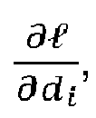
- In the second stage, the score matrix S is computed (according to Eq. 1) as well as the loss function ℓ = L(D,Y), and the gradient of the loss function with respect to the global feature descriptors

- During the last stage, the global feature descriptors are recomputed, this time storing the intermediary tensors. This operation occupies a lot of memory, but it can now be performed image by image. Given the global feature descriptor di for the image Ii and the gradient of the loss function with respect to this global feature descriptor
- The algorithm for efficient training of the gradients for an arbitrary number of images in the set (batch) of training images works as follows:
- Inputs: training batch

- for i in 1..B; do
compute di ← fΘ (Ii ) - create

- create Y ∈ {0,1} B×B such that Yij = 11[yi = yj ]
- ℓ ← L(D,Y) # compute the loss
- compute

- init

- for i in 1..B; do
- compute di ← fΘ (Ii )
- compute

- accumulate
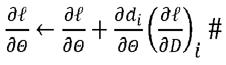
- update

- First, the different datasets used in experiments performed according to an embodiment will be discussed. Then, key parameters of the disclosed embodiments are identified and compared to other results obtained in the field.
- The original Landmarks dataset contains 213,678 images divided into 672 classes. However, since this dataset has been created semi-automatically by querying a search engine, it contains a large number of mislabeled images. An automatic cleaning process can be performed to clean this dataset, and the result is called the Landmarks-clean dataset. It contains 42,410 images and 586 landmarks, and it is the version used to train the CNN in all the experiments discussed below.
- The Revisited Oxford (Oxford) and Revisited Paris (
 Paris) datasets contain 4,993 and 6,322 images respectively, with 70 additional images for each that are used as queries (see
Fig. 4 for example queries). These images are further labeled according to the difficulty in identifying which landmark they depict (Easy, Hard, Unclear, and Negative). These categories are then used to determine three evaluation protocols for these datasets: - Easy: Easy images are considered positive, Hard and Unclear are ignored.
- Medium: Easy and Hard images are considered positive, Unclear are ignored.
- Hard: Hard images are considered positive, Easy and Unclear are ignored.
- Optionally, a set of 1 million distractor images (1M) can be added to each dataset to make the task more realistic. Since these new datasets are essentially updated versions of the original Oxford and Paris datasets, with the same characteristics but more reliable ground-truth labels, these revisited versions have been used in the experiments discussed below.

- The CNN has been trained using stochastic gradient on the public Landmarks-clean dataset. In all experiments discussed below, a ResNet-101 CNN pre-trained on ImageNet is used as a backbone (i.e., a starting state of the CNN before beginning the training phase). ResNet-101 is a specific instantiation of a CNN architecture making use of 101 convolution layers, from the paper "Deep residual learning for image recognition" by K. He, X. Zhang, S. Ren, and J. Sun, in Conference on Computer Vision and Pattern Recognition, CVPR, 2016. Further, the original final layer of the ResNet-101 CNN (which was specific to a classification algorithm) has been replaced by a generalized-mean pooling (GeM) layer. The GeM layer is a particular type of layer which performs global feature pooling (i.e. it transforms an image of variable width and height into a fixed size vector). The GeM layer contains a single trainable parameter which is trained through back-propagation of the gradients, as the rest of the network parameters.
- In an embodiment, the above REsNet-101 network is trained according to the Adam optimizer of D.P. Kingma and J. Ba: "Adam: a method for stochastic optimization", arXiv preprint, 2014. Unless stated otherwise, the following parameters are used: the weight decay (which specifies how the learnable parameters are updated during back-propagation) is set to 10-6, and the set of training images is augmented by generating additional training images through standard data augmentation (by applying e.g., color jittering, random scaling, rotation and cropping). For instance, one actual training image is slightly transformed by applying some slight color noise to it (so called "color jittering"), which makes a new, very similar image. Training images are cropped to a fixed size of 800 × 800, but during test, the original images (unscaled and undistorted) are fed into the CNN.
- In the art, using multiple scales is a common practice to improve test performance. It consists in feeding the input image several times in the CNN, each time with a different scaling (resolution) to get slightly different multiple global representations which are complementary. These multiple representation may be averaged to get an improved final image representation. In the implementation according to the embodiments described above, however, it has been observed that using multiple scales at test time did not lead to any significant improvement. Operating at a single scale makes the global feature descriptor extraction about 3 times faster than state-of-the-art methods for a comparable network backbone.
- The choice of other parameters will now be discussed based on different experimental studies.
- It has been found that the highest learning rate that does not result in divergence gives best results. A linearly decaying learning rate starting from 10-4 and decreasing to 0 after 200 iterations has been used.
- The APQ loss function depends on the number of quantization bins M in Eq. 7. The performance achieved for different values of M is plotted in
Fig. 5 , which shows that this parameter has little impact on the performance of the loss function for training the CNN. M = 20 quantization bins have been used in all other experiments. - The experimental results show that larger batch sizes lead to better results, as illustrated in
Fig. 6 . The performance saturates beyond 4096, and training significantly slows down as well. Accordingly, batches of 4096 images are used in all subsequent experiments. - Each batch is constructed by sampling random images from each dataset class (all classes are hence represented in a single batch). Experiments showed that sampling the classes did not lead to any difference, as illustrated by
Fig. 7 . Due to the dataset imbalance, certain classes are constantly over-represented at the batch level. To counter-balance this situation, a weight has been introduced in Eq. 12 to weight equally all classes inside a batch. Two CNNs have been trained with and without this weighting. The results are presented inFig. 8 . The improvement in terms of mean average precision with class weighting is around +2% and shows the importance of this balancing. - A bias can occur in the ranking of the images according to their similarities if "ties" are present in the embedding space. In this context, ties relate to images having global feature descriptors in the embedding space that are at the same distance to the query image and therefore equally similar to the query image. In such a case, an uncertainty occurs regarding how these images should be ranked in the final result. In order to minimize this bias, a tie-aware version of the APQ loss function (called APT) has been developed for the specific case of ranking integer-valued Hamming distances and also applied to real-valued distances. However, for implementing these tie-aware versions of APQ, approximations are necessary. A simplified tie-aware AP loss function has also been used and its efficiency has been compared to the one of APQ. The APT is computed in a way similar to APQ in Eq. 11, but the precision is replaced by a more accurate approximation:

- The absolute difference in terms of mean average precision is presented in
Fig. 9 , which shows that the mAPQ loss function, straightforwardly derived from the definition of AP, consistently outperforms the tie-aware formulation by a small but significant margin. This may be due to the fact that the tie-aware formulation used in practical implementations is in fact an approximation of the theoretical tie-aware AP. Accordingly, the mAPQ loss function has been used in all subsequent experiments. - Descriptor whitening is frequently used in the art to improve the performance of global feature descriptors. It consists in multiplying a global feature descriptor (extracted e.g. from the Landmarks dataset described above) by a matrix obtained using principal component analysis (PCA) on the image representations of the training set. A PCA returns the eigenvalues (Dx1 vector) and the eigenvectors (DxD matrix). Instead of using only the DxD eigenvector matrix, in one embodiment, a PCA matrix M = diagonal(sqrt(eigenvalues)) * eigenvectors, where diagonal() creates a diagonal matrix from a vector and sqrt() computes the element-wise square-root. The global feature descriptors are then normalized at test time using the computed PCA. The above defined square-rooted PCA was found to be more effective. Whitening has been used in all subsequent experiments.
- Embodiments will now be described in detail in relation to the above and by reference to the drawings of
Figs. 10 to 12 . In the following embodiments, reference is made to training and use of a CNN. According to exemplary embodiments, a deep feedforward network (DFN) or a convolutional forward network (CFN) can be used. -
Fig. 10 is a functional block diagram illustrating a computer-implemented method for training a CNN according to an embodiment. It begins atstep 1002, at which a batch (or a set) of training images is obtained. Obtaining the training images encompasses that they can be received from a user dealing with the training phase of the CNN or from any memory location (e.g. a local or remote computing system, a local or remote database, a cloud storage or any other memory location known in the field) on which they are stored. Alternatively, the images of the batch can be retrieved by a user or automatically retrieved from any of these memory locations. The images of the batch used for the training phase are known, and in particular their respective similarities are known, thereby providing the ground-truth image relevance mentioned above. The ground-truth image relevance consists for example in a set of known binary ground-truth labels (one label for each pair of images of the batch), each label of a given pair of images informing whether these images are similar (in which case, the label is equal to 1) or not (in which case, the label is equal to 0). For example, the received batch can be one of the datasets of known images mentioned above, i.e.Paris or Oxford. In an embodiment, the training images of the batch are high-resolution images of more than 1 Megapixels.
- At
step 1004, a global feature descriptor is computed in an embedding space for each image of the received batch. This is achieved by inputting each image of the batch into the CNN to be trained and getting the corresponding global feature descriptor as output of the CNN. As explained above, the global feature descriptors are vectors defined in a multi-dimensional space called the embedding space, and each global feature descriptor describes uniquely the corresponding image in the embedding space. As mentioned above, in an embodiment, the CNN can be a ResNet CNN, for example a ResNet-101, which has 101 convolution layers. However, any number of layers higher than 20 layers, and preferably around 100 layers, may be used as well. Further, the original CNN (i.e., the CNN with the original values of its learnable parameters before the training phase begins) can be pre-trained on ImageNet. Alternatively, any available CNN that has been trained for classification tasks can also be used as original CNN. - At
step 1006, a similarity is computed between each given pair of images of the batch based on a distance between the global feature descriptors in the embedding space. Any known distance metric can be used to compute these similarities. For example, an Euclidean metric can be used to determine the distance between two global feature descriptors in the embedding space, and the similarity between two images can be a value proportional to the Euclidean distance between the corresponding global feature descriptors. However, any other definition of the similarity can be used, based on any definition of the distance between global feature descriptors in the embedding space, without departing from the scope of the embodiments disclosed herein. - At
step 1008, a ranking function R is applied to the images of the batch to sort them based on their similarities. For example, each image of the batch is considered to be an initial query image, and the remaining images of the batch are ranked (or sorted) according to their similarities to the query image. The images of the batch can be ranked by decreasing or by increasing similarity. An example of the ranking obtained in this step for a given query image can be found inFig. 4 discussed above, at different training stages of the CNN (i.e., at different numbers of iterations of the training method illustrated inFig. 10 ). - At
step 1010, the quality of the obtained rankings is evaluated according to an average precision (AP) ranking evaluation metric. As relative similarities between the images of the batch are known (through e.g. a set of given binary ground-truth labels, as explained above), in an embodiment, evaluating the quality of a ranking is performed by computing an average precision of the ranking compared to the known relative similarities between the images of the batch. In an embodiment, the AP is the sum over all images of the product of a precision at rank k times an incremental recall from ranks k-1 to k, where the precision at rank k is the proportion of relevant images found in the k first indexes of the ranking, and the incremental recall is the proportion of relevant images found at rank k out of a total of relevant images. For details on this step and on the formulation of AP, it is referred to the section "Definitions" above. - At
step 1012, the AP is reformulated into a differentiable AP called quantized AP (or APQ) using histogram binning and quantization. Reformulating the AP ranking evaluation metric into APQ comprises replacing the indicator function in the AP ranking evaluation metric by a quantization function δ being a set of triangular kernels each centered around a bin center bm of an histogram binning. For details on this step, it is referred to the section "Quantization function" above. - At
step 1014, the mean of APQ (mAPQ) over the batch of training images is computed. For details on this step, it is referred to the section "Training procedure" above. - At (optional)
step 1015, the listwise ranking loss function L(D,Y) as defined above in Eq. 13 is computed based on mAPQ. The listwise ranking loss function is a loss function adapted to optimize ranking during the training phase of the CNN, which takes a variable number of training images at the same time and optimizes their ranking jointly, wherein the listwise ranking loss function is minimal when the variable number of training images has been ranked correctly by the ranking function during the training phase. - At
step 1016, each given learnable parameter of the CNN is adapted through back-propagation of the gradient of mAPQ with respect to the given learnable parameter. - Finally, at
step 1018, it is determined whether the listwise ranking loss function based on mAPQ has converged towards a minimum (or equivalently whether mAPQ converges towards a maximum), meaning that the ranking function optimally ranks the training images and obtains a result similar to the expected result (complying with the known ground-truth image relevance). For example, this determination can be performed by comparing the newly computed value of mAPQ instep 1014 with the previous value of mAPQ (or the respective new and previous values of the corresponding loss function) and determining whether these values are equal or at least whether the difference between the new value and the previous value falls below a predetermined threshold. However, any other method for determining convergence can be used without departing from the scope of the present disclosure. - If it is determined that the listwise ranking loss function has converged towards a minimum, the method ends at
step 1020 at which the training phase is concluded. The trained CNN can then be applied to image retrieval with any set of images, as will be described in detail in relation withFig. 11 . However, if it is determined that the listwise ranking loss function has not converged yet, thetraining steps 1004 to 1016 are repeated until convergence is achieved. - It is noted that though the steps of the method illustrated in
Fig. 10 have been described in a given order, this order is not meant to be restrictive and all the alternative embodiments that a skilled person would consider to implement the same general idea are also contemplated without departing from the scope of the present disclosure. For example, the determiningstep 1016 could also be performed immediately afterstep 1014 and a last adaptation of the learnable parameters could thereby be avoided in case convergence is achieved, since this last adaptation will not modify (or at least not substantially modify) the learnable parameters once convergence has been achieved. -
Fig. 11 is a functional block diagram illustrating a method for image retrieval in response to the reception of a query image according to an embodiment. This method can be performed by applying the trained CNN (obtained at the end of the method ofFig. 10 ,) to an unknown set of images distinct from the training batch of images as soon as the training phase illustrated instep 1020 ofFig. 10 has been concluded, i.e. as soon as mAPQ has converged, which means that the learnable parameters of the CNN have been learned successfully and that the CNN is now ready for general image retrieval tasks. - The steps performed for responding to a query image are at least in part similar to the steps performed during the training phase described in relation with
Fig. 10 , but without having to evaluate the ranking function anymore, nor having to adapt the learnable parameters of the CNN. On the contrary, it is now considered that once the training phase has been successfully fulfilled, the measure of similarities between the images based on the distances between their corresponding global feature descriptors in the embedding space is now optimal. In other words, it is now considered that the function defining the global feature descriptor of an image, as encoded within the CNN (through the final values of its learnable parameters obtained at the end of the training phase), is now optimal for comparing input images and ranking them according to a similarity measure. - In detail, at
step 1102, a (potentially unknown) query image is obtained. Obtaining the query image encompasses as well embodiments in which the query image is received as embodiments in which the query image is retrieved. This query image may be received from a user or from any other source, manually or automatically. Alternatively, it may be retrieved by the user or automatically by programming means like e.g. an application. The source may be local or remote, and may be e.g. a database or any type of digital memory or any source from which an image can be digitalized. Alternatively, the source itself may be an application or any type of program code having access to images stored in memory. The query image may pertain to the batch of training images, but may be as well any new image that has never been input into the CNN before. The query image may be a high-resolution image of at least 65000 pixels. - At
step 1104, the query image is input into the CNN which has been previously trained (e.g. according to the method ofFig. 10 ), and a corresponding global feature descriptor is output by the trained CNN. In an embodiment, the learnable parameters of the CNN have been learned by training the CNN on a known batch of training images using a listwise ranking loss function directly optimizing a quantized mean average precision, mAPQ, ranking evaluation metric. - At
step 1106, a similarity is measured between the query image and each other image previously input into the CNN, based on a distance in the embedding space between the global feature descriptor of the query image and the respective global feature descriptors of the other images. - At
step 1108, the images that have been previously input into the CNN are ranked based on their similarity to the query image, for example ranked by decreasing similarity. - Finally, at
step 1110, a set of images is selected based on the similarity of the images of the set to the query image and a set of identifiers representative of the set of images is output. The set of identifiers may identify the images themselves or other data associated with the images such as a class (for image categorization), an object such as a person's name (for facial/retinal recognition), or a location (from location data associated with metadata of images) etc. Optionally, these identifiers and/or the selected set of images itself may then be provided to the user or to any other target person or target location in response to his/her query. For example, all the images previously input into the CNN, or only a subset of the images for which the similarity to the query image is above a predetermined threshold, can be provided. Alternatively, only a predetermined number of the most similar images could be provided. In all these cases, in an embodiment, the images can be ranked by decreasing similarity. Alternatively, embodiments are also contemplated where the resulting set of images provided to the user is not ranked, or ranked by increasing similarity, or according to any other criterion independent of the similarity. - It is noted that these examples are not meant to be restrictive and that all the alternative embodiments that a skilled person would consider in order to implement the same general idea are also contemplated without departing from the scope of the present disclosure.
-
Fig. 12 is a functional block diagram illustrating a method for optimizing one iteration of the training of the CNN over a large number of input images according to an embodiment. It corresponds to the algorithm described above in the section "Training for high-resolution images" that can be applied to implementsteps 1004 to 1016 of the training phase of the CNN described above in relation withFig. 10 , for adapting the learnable parameters of the CNN. This three-stage algorithm is optimized to spare memory and time, since in view of the fact that the CNN is trained with high-resolution images of arbitrary high size and resolution, computing the gradients of the loss function with respect to all the learnable parameters of the CNN over all the images of the training batch would be infeasible in practice. The overall idea behind this algorithm is to use the chain rule in the computation of the gradients (in the second stage of the algorithm) in order to compute the gradients recurrently by successively adding the contribution of each given image to the gradients, one image at a time, thereby freeing the memory of the computations made for one image before treating the contribution of the next image to the gradients. - It begins with a first stage at
step 1202, at which the global feature descriptors of all the images of the training batch are computed, but where all the intermediary tensors obtained during the computation are discarded. - In a second stage at
step 1204, the similarities between each pair of images in the batch are computed, as well as the listwise ranking loss function (or, equivalently, mAPQ), and the gradients of the loss function (or, equivalently, of mAPQ) with respect to the global feature descriptors of the images of the batch. However, no back-propagation of the gradients to adapt the learnable parameters is performed at that time. - On the contrary, in a third stage, a loop is initiated over the images in the batch (through the determination, at
step 1212, whether there are still one or more images in the batch that have not been treated yet), and for each given image of the batch (selected in step 1206), the following steps are performed: first, atstep 1208, its global feature descriptor is recomputed, the gradients of the loss function (or, equivalently, of mAPQ) with respect to the learnable parameters of the CNN are computed, and this time the intermediary tensors obtained during the computation are kept in memory; secondly, atstep 1210, for each learnable parameter of the CNN, a gradient is computed as follows: after an initialization of all gradients to zero before the first image is treated in this third stage, the contribution of the given image to this gradient is added to the previous value of this gradient. Once all the images of the batch have been treated one by one, the final gradients with respect to each learnable parameter have been fully computed and they can be back-propagated atstep 1214 to adapt the learnable parameters. - All the
steps 1202 to 1214 of this algorithm have to be repeated over a number of iterations until convergence is achieved, i.e. until it is determined at thefinal step 1018 of the training phase illustrated inFig. 10 that either mAPQ has reached a maximum, or equivalently that the listwise ranking loss function has reached a minimum. In an embodiment, mAPQ is the mean over the batch of training images of a quantized average precision ranking evaluation metric, APQ, which is a quantized version of an average precision, AP, ranking evaluation metric that has been rendered differentiable using histogram binning and quantization. - As an improvement to the previous algorithm, at the end of
step 1202, the intermediary tensors of the last image that has been treated can be kept in memory and this image can be the first one to be selected instep 1206, in order to avoid an unnecessary re-computation of the global feature descriptor of the last image. - It is noted that the order and the number of the steps of
Fig. 12 are illustrative. They are not meant to be restrictive and all the alternative embodiments that a skilled person would consider in order to implement the same general idea are also contemplated without departing from the scope of the present disclosure. For example, the loop performed on the images of the batch can be implemented according to any alternative formulation that would fall within the usual skills of a person skilled in the art. - The results obtained with the above described model will now be compared with the state of the art. The top part of Table 1 summarizes the performance of the best-performing methods on the datasets listed in section 5.1 without query or database expansion. The notation of (Radenovic et al. 2018) is used as this helps to clarify important aspects about each method. Namely, generalized-mean pooling (Radenovic, Tolias, and Chum 2018) is denoted by GeM and the R-MAC pooling (Tolias, Sicre, and Jegou 2016) is denoted by R-MAC. The type of loss function used to train the model is denoted by CL for the contrastive loss, TL for the triplet loss, AP for the APQ loss described above, and O if no loss is used (i.e. off-the-shelf features).
- Overall, embodiments according to the described model outperform the state of the art by 1% to 5% on all datasets and protocols. For instance, the described model is more than 4 points ahead of the best reported results (Radenovic, Tolias, and Chum 2018) on the hard protocol ofOxford and
 Paris. This is remarkable since the described model uses a single scale at test time (i.e. the original test images), whereas other methods boost their performance by pooling feature descriptors computed at several scales. In addition, the trained CNN described above does not undergo any special pre-training step (it has been initialized with ImageNet-trained weights), again unlike most competitors from the state of the art. Empirically one observes that the APQ loss renders such pre-training stages obsolete. Finally, the training time is also considerably reduced: training the described CNN from scratch takes a few hours on a single P40 GPU.
- Further, results with query expansion (QE) and database augmentation (DBA) are reported at the bottom of Table 1. The α-weighted versions of (Radenovic, Tolias, and Chum 2018) with α = 2 and k = 10 nearest neighbors for both QE and DBA are used in all experiments. The described model with QE outperforms other methods also using QE in 6 protocols out of 8. Using simple α-expansion based DBA, it is also able to outperform the comparatively expensive diffusion-based augmentation scheme (Iscen et al. 2017) on the Oxford dataset by a large margin (+5% on the medium protocol, +9% on the hard protocol), while staying competitive onParis.

- Finally, the results obtained with the trained CNN described above are on par with those of the method proposed by Noh et al. (Noh et al. 2017), which is based on local descriptors. Even though the described method relies on global descriptors, hence lacking any geometric verification, it still outperforms it on theOxford and
 Paris datasets without added distractors.
Table 1: All global representations are learned from a ResNet-101 backbone, with varying pooling layers and fine-tuning losses. Abbreviations: (O) off-the-shelf features; (CL) fine-tuned with contrastive loss; (TL) fine-tuned with triplet loss; (AP) fine-tuned with mAP loss (according to the described embodiments); (SP) spatial verification with RANSAC; (αQE) weighted query expansion (Radenović, Tolias, and Chum 2018); (DFS) query expansion with diffusion (Iscen et al. 2017). Medium Hard Oxf Oxf+1 M
 Par
Par Par+1 M
 Oxf
Oxf Oxf+1 M
 Par
Par Par+1 M
Local descriptors HesAff-rSIFT-ASMK* + SP (Radenović et al. 2018) 60.6 46.8 61.4 42.3 36.7 26.9 35.0 16.8 DELF-ASMK * + SP (Noh et al. 2017) 67.8 53.8 76.9 57.3 43.1 31.2 55.4 26.4 Global representations MAC (O) (Tolias, Sicre, and Jégou 2016) 41.7 24.2 66.2 40.8 18.0 5.7 44.1 18.2 SPoC (O) (Babenko and Lempitsky 2015) 39.8 21.5 69.2 41.6 12.4 2.8 44.7 15.3 CroW (O) (Kalantidis, Mellina, and Osindero 2016) 42.4 21.2 70.4 42.7 13.3 3.3 47.2 16.3 R-MAC (O) (Tolias, Sicre, and Jégou 2016) 49.8 29.2 74.0 49.3 18.5 4.5 52.1 21.3 R-MAC (TL) (Gordo et al. 2017) 60.9 39.3 78.9 54.8 32.4 12.5 59.4 28.0 GeM (O) (Radenović, Tolias, and Chum 2018) 45.0 25.6 70.7 46.2 17.7 4.7 48.7 20.3 GeM (CL) (Radenović, Tolias, and Chum 2018) 64.7 45.2 77.2 52.3 38.5 19.9 56.3 24.7 GeM (AP) [ described embodiments] 67.5 47.5 80.1 52.5 42.8 23.2 60.5 25.1 Query expansion R-MAC (TL) + αQE (Gordo et al. 2017) 64.8 45.7 82.7 61.0 36.8 19.5 65.7 35.0 GeM (CL) + αQE (Radenović, Tolias, and Chum 2018) 67.2 49.0 80.7 58.0 40.8 24.2 61.8 31.0 GeM (AP) [described embodiments] + αQE 71.4 53.1 84.0 60.3 45.9 26.2 67.3 32.3 Query and database expansion R-MAC (TL) + DFS (Gordo et al. 2017) 69.0 56.6 89.5 83.2 44.7 28.4 80.0 70.4 GeM (CL) + DFS (Radenović, Tolias, and Chum 2018) 69.8 61.5 88.9 84.9 40.5 33.1 78.5 71.6 GeM (AP) [ described embodiments] + αQE + αDBA 75.3 - 86.9 - 53.8 - 73.4 - - While some specific embodiments have been described in detail above, it will be apparent to those skilled in the art that various modifications, variations and improvements of the embodiments may be made in the light of the above teachings and within the content of the appended claims without departing from the intended scope of the embodiments. In addition, those areas in which it is believed that those of ordinary skill in the art are familiar have not been described herein in order not to unnecessarily obscure the embodiments described herein. Accordingly, it is to be understood that the embodiments are not to be limited by the specific illustrative embodiments, but only by the scope of the appended claims.
- Although the above embodiments have been described in the context of method steps, they also represent a description of a corresponding component, module or feature of a corresponding apparatus or system.
- Some or all of the method steps may be implemented by a computer in that they are executed by (or using) a processor, a microprocessor, an electronic circuit or processing circuitry.
- The embodiments described above may be implemented in hardware or in software. The implementation can be performed using a non-transitory storage medium such as a computer-readable storage medium, for example a floppy disc, a DVD, a Blu-Ray, a CD, a ROM, a PROM, and EPROM, an EEPROM or a FLASH memory. Such computer-readable media can be any available media that can be accessed by a general-purpose or special-purpose computer system.
- Generally, embodiments can be implemented as a computer program product with a program code or computer-executable instructions, the program code or computer-executable instructions being operative for performing one of the methods when the computer program product runs on a computer. The program code or the computer-executable instructions may, for example, be stored on a computer-readable storage medium.
- In an embodiment, a storage medium (or a data carrier, or a computer-readable medium) comprises, stored thereon, the computer program or the computer-executable instructions for performing one of the methods described herein when it is performed by a processor. In a further embodiment, an apparatus comprises one or more processors and the storage medium mentioned above.
- In a further embodiment, an apparatus comprises means, for example processing circuitry like e.g. a processor communicating with a memory, the means being configured to, or adapted to, perform one of the methods described herein.
- A further embodiment comprises a computer having installed thereon the computer program or instructions for performing one of the methods described herein.
- The above-mentioned methods and embodiments may be implemented within an architecture such as illustrated in
Fig. 13 , which comprisesserver 100 and one or more client devices 102 that communicate over a network 104 (which may be wireless and/or wired) such as the Internet for data exchange.Server 100 and the client devices 102 include a data processor 112 and memory 113 such as a hard disk. The client devices 102 may be any device that communicates withserver 100, includingautonomous vehicle 102b,robot 102c,computer 102d, orcell phone 102e. - More precisely in one embodiment, the query image obtained in
step 1102 of the method of performing image retrieval corresponds to a query initiated by client device 102. The query is processed atserver 100, which returns processed identifiers representative of the set of images to client device 102. In an alternate embodiment, the query can be processed at the client device 102 that initiated the query. The method for training learnable parameters of a CNN may also be performed atserver 100 or in an alternate embodiment at a different server or in another alternate embodiment at the client device 102.
Claims (15)
- A computer-implemented method of performing image retrieval, the method comprising:obtaining (1102) a query image;computing (1104) a global feature descriptor of the query image by inputting the query image into a trained convolutional neural network, CNN, and obtaining the global feature descriptor in an embedding space as output, wherein learnable parameters of the CNN have been learned by training the CNN on a known batch of training images using a listwise ranking loss function directly optimizing a quantized mean average precision, mAPQ, ranking evaluation metric;computing (1106) a similarity between the query image and images that have been previously input into the CNN based on a distance in the embedding space between the global feature descriptor of the query image and the global feature descriptors of the images that have been previously input into the CNN;applying (1108) a ranking function to the images that have been previously input into the CNN to obtain a ranking of these images based on their similarity to the query image; andselecting (1110) a set of images based on their similarity to the query image and outputting a set of identifiers representative of the set of images.
- The method of claim 1, wherein the CNN is a ResNet network with more than 20 layers, preferably around 100 layers.
- The method of claim 1 or 2, wherein the training images of the batch are high-resolution images with a size of at least 65000 pixels.
- The method of one of claims 1 to 3, wherein the listwise ranking loss function is a loss function adapted to optimize ranking during a training phase of the CNN, which takes a variable number of training images at the same time and optimizes their ranking jointly, wherein the listwise ranking loss function is minimal when the variable number of training images has been ranked correctly by the ranking function during the training phase.
- The method of one of claims 1 to 4, wherein training the CNN on a known batch of training images includes:a1) obtaining (1002) a batch of training images;b1) computing (1004) a global feature descriptor of each given image of the batch in the embedding space by inputting the given image into the CNN and obtaining the global feature descriptor of the given image as output of the CNN;c1) computing (1006) a similarity between each given pair of images of the batch based on a distance between the global feature descriptors of the images of the given pair in the embedding space;d1) applying (1008) a ranking function to the images of the batch to obtain a ranking of the images of the batch based on their similarities;e1) evaluating (1010) the quality of the ranking using an average precision, AP, ranking evaluation metric, the AP ranking evaluation metric containing a non-differentiable indicator function;f1) reformulating (1012) the AP ranking evaluation metric into a differentiable AP ranking evaluation metric called quantized AP, APQ, using histogram binning and quantization;g1) computing (1014) a mean of APQ, which is the quantized mean average precision mAPQ, over the batch of training images;h1) for each given learnable parameter of the CNN, adapting (1016) the given learnable parameter of the CNN by back-propagating a gradient of mAPQ with respect to the given learnable parameter;i1) determining (1018) whether the listwise ranking loss function based on mAPQ has reached a minimum;if it is determined that the listwise ranking loss function has not reached a minimum, repeating the previous steps b1) to i1) until it is determined that mAPQ has reached a maximum; andif it is determined that the listwise ranking loss function has reached a minimum, concluding (1020) the training phase.
- The method of claim 5, further comprising computing (1015) the listwise ranking loss function based on mAPQ as being equal to 1 - mAPQ, and wherein determining whether the listwise ranking loss function based on mAPQ has reached a minimum is equivalent to determining that mAPQ has reached a maximum.
- The method of claim 5 or 6, wherein reformulating the AP ranking evaluation metric into APQ comprises replacing the indicator function in the AP ranking evaluation metric by a quantization function δ being a set of triangular kernels each centered around a bin center bm of a histogram binning.
- The method of one of claims 5 to 7, wherein relative similarities between the images of the batch are known, and wherein evaluating the quality of the ranking using an average precision, AP, ranking evaluation metric is performed by computing an average precision of the ranking compared to the known relative similarities between the images of the batch.
- The method of one of claims 5 to 8, where the AP is the sum over all images of the product of a precision at rank k times an incremental recall from ranks k-1 to k, where the precision at rank k is the proportion of relevant images found in the k first indexes of the ranking, and the incremental recall is the proportion of relevant images found at rank k out of a total of relevant images.
- The method of one of claims 5 to 9, wherein training the CNN on a known batch of training images is performed in a memory-efficient way through a three-stage algorithm comprising:a2) computing (1004; 1202) a global feature descriptor of each given image of the batch in the embedding space further includes discarding intermediary tensors obtained during the computation of the global feature descriptor in the memory;b2) computing (1006; 1204) a similarity between each given pair of images of the batch;c2) computing (1204) the listwise ranking loss function, and gradients of the loss function with respect to the global feature descriptors, without performing back-propagation of the gradients to the learnable parameters at that time;d2) processing all the images of the batch by:a') selecting (1206) a given image of the batch;b') re-computing (1208) the corresponding global feature descriptor of the given image and the gradients of the loss function with respect to the learnable parameters of the CNN, and keeping the intermediary tensors in the memory;c') for each given learnable parameter of the CNN, adding (1210) the contribution of the given image to an overall gradient of the loss function with respect to the given learnable parameter; andrepeating steps a') to c') until it is determined (1212) that there is no remaining unselected image in the batch;e2) once it is determined that there is no remaining unselected image in the batch, adapting (1016; 1214) the given learnable parameters of the CNN by back-propagating each overall gradient of the loss function to adapt the corresponding learnable parameter of the CNN; andf2) repeating steps a2) to e2) of the algorithm until it is determined that the loss function has reached a minimum.
- The method of one of claims 1 to 10, wherein selecting a set of images comprises selecting a predefined number of images most similar to the query image in a ranked order according to their similarity to the query image in decreasing order.
- A computer-implemented method for training learnable parameters of a convolutional neural network, CNN, on a known batch of training images in a memory-efficient way through a three-stage algorithm, the method comprising:a3) computing (1202) a global feature descriptor for each image of the batch in the embedding space, but discarding intermediary tensors obtained during the computation of the global feature descriptor in the memory;b3) computing (1204) a similarity between each pair of images in the batch, a listwise ranking loss function, and gradients of the loss function with respect to the global feature descriptors, without performing back-propagation of the gradients to the learnable parameters at that time;c3) processing all the images of the batch by:a') selecting (1206) a given image of the batch;b') re-computing (1208) the corresponding global feature descriptor of the given image and the gradients of the loss function with respect to the learnable parameters of the CNN, and keeping the intermediary tensors in the memory;c') for each given learnable parameter of the CNN, adding (1210) the contribution of the given image to an overall gradient of the loss function with respect to the given learnable parameter; andrepeating steps a') to c') until it is determined (1212) that there is no remaining unselected image in the batch;d3) once it is determined that there is no remaining unselected image in the batch, back-propagating (1214) each overall gradient of the loss function to adapt the corresponding learnable parameter of the CNN; ande3) repeating steps a3) to d3) of the algorithm until it is determined that the listwise ranking loss function has reached a minimum.
- The method of claim 12, wherein determining that the listwise ranking loss function has reached a minimum is equivalent to determining whether a quantized mean average precision ranking evaluation metric, mAPQ, has reached a maximum, and wherein mAPQ is the mean over the batch of training images of a quantized average precision ranking evaluation metric, APQ, which is a quantized version of an average precision, AP, ranking evaluation metric that has been rendered differentiable using histogram binning and quantization.
- One or more computer-readable media storing thereon computer-executable instructions that, when carried out by a processor, cause the processor to perform the method of one of claims 1 to 13.
- An apparatus comprising processing circuitry, the processing circuitry being configured to perform the method of one of claims 1 to 13.
Priority Applications (3)
| Application Number | Priority Date | Filing Date | Title |
|---|---|---|---|
| EP19305542.3A EP3731154A1 (en) | 2019-04-26 | 2019-04-26 | Training a convolutional neural network for image retrieval with a listwise ranking loss function |
| US16/787,594 US11521072B2 (en) | 2019-04-26 | 2020-02-11 | Training a convolutional neural network for image retrieval with a listwise ranking loss function |
| KR1020200046792A KR20200125468A (en) | 2019-04-26 | 2020-04-17 | Training a convolutional neural network for image retrieval with a listwise ranking loss function |
Applications Claiming Priority (1)
| Application Number | Priority Date | Filing Date | Title |
|---|---|---|---|
| EP19305542.3A EP3731154A1 (en) | 2019-04-26 | 2019-04-26 | Training a convolutional neural network for image retrieval with a listwise ranking loss function |
Publications (1)
| Publication Number | Publication Date |
|---|---|
| EP3731154A1 true EP3731154A1 (en) | 2020-10-28 |
Family
ID=67139676
Family Applications (1)
| Application Number | Title | Priority Date | Filing Date |
|---|---|---|---|
| EP19305542.3A Pending EP3731154A1 (en) | 2019-04-26 | 2019-04-26 | Training a convolutional neural network for image retrieval with a listwise ranking loss function |
Country Status (3)
| Country | Link |
|---|---|
| US (1) | US11521072B2 (en) |
| EP (1) | EP3731154A1 (en) |
| KR (1) | KR20200125468A (en) |
Cited By (9)
| Publication number | Priority date | Publication date | Assignee | Title |
|---|---|---|---|---|
| CN113033704A (en) * | 2021-04-22 | 2021-06-25 | 江西理工大学 | Intelligent judging method for copper converter converting copper making period end point based on pattern recognition |
| CN113223068A (en) * | 2021-05-31 | 2021-08-06 | 西安电子科技大学 | Multi-modal image registration method and system based on depth global features |
| CN114090816A (en) * | 2021-11-23 | 2022-02-25 | 中国科学技术大学 | Visual reordering method, system, equipment and storage medium for image retrieval |
| CN114187610A (en) * | 2021-12-02 | 2022-03-15 | 南京理工大学 | Low-cost pedestrian re-identification method based on deep active learning |
| CN114429192A (en) * | 2022-04-02 | 2022-05-03 | 中国科学技术大学 | Image matching method and device and electronic equipment |
| US20230091062A1 (en) * | 2020-03-10 | 2023-03-23 | Sensen Networks Group Pty Ltd. | Systems and Methods for Image-Based Location Determination and Parking Monitoring |
| CN117556273A (en) * | 2024-01-05 | 2024-02-13 | 支付宝(杭州)信息技术有限公司 | A method and device for calculating contrast loss through multiple graphics processors |
| CN120045737A (en) * | 2025-01-24 | 2025-05-27 | 清华大学深圳国际研究生院 | Two-stage place recognition method based on similarity constraint depth hash |
| CN120634934A (en) * | 2025-08-13 | 2025-09-12 | 崂山国家实验室 | Underwater image enhancement method and system based on vision-text fusion |
Families Citing this family (44)
| Publication number | Priority date | Publication date | Assignee | Title |
|---|---|---|---|---|
| GB2585005B (en) * | 2019-06-24 | 2021-06-23 | Roadmetric Ltd | Training a machine to recognize a motor vehicle driver using a mobile device |
| EP3767536B1 (en) * | 2019-07-17 | 2025-02-19 | Naver Corporation | Latent code for unsupervised domain adaptation |
| CN112362679B (en) * | 2019-07-23 | 2024-06-04 | 纬创资通股份有限公司 | Image recognition device, image recognition method and computer program product thereof |
| CN112308816B (en) * | 2019-07-23 | 2024-02-06 | 纬创资通股份有限公司 | Image recognition device, image recognition method and storage medium thereof |
| CN112304952B (en) * | 2019-07-23 | 2024-04-02 | 纬创资通股份有限公司 | Image recognition device, image recognition method and computer program product thereof |
| US10943353B1 (en) | 2019-09-11 | 2021-03-09 | International Business Machines Corporation | Handling untrainable conditions in a network architecture search |
| US11023783B2 (en) * | 2019-09-11 | 2021-06-01 | International Business Machines Corporation | Network architecture search with global optimization |
| CN114930824B (en) * | 2020-01-08 | 2025-09-16 | 谷歌有限责任公司 | Depth palette prediction |
| JP7268069B2 (en) * | 2020-02-21 | 2023-05-02 | アクタピオ,インコーポレイテッド | LEARNING DEVICE, LEARNING METHOD, LEARNING PROGRAM, EVALUATION DEVICE, EVALUATION METHOD, AND EVALUATION PROGRAM |
| US11468294B2 (en) * | 2020-02-21 | 2022-10-11 | Adobe Inc. | Projecting images to a generative model based on gradient-free latent vector determination |
| EP4009195B1 (en) * | 2020-12-01 | 2025-04-30 | Airbus Defence and Space SAS | Method for storing information with indexed image fields and method for retrieving the same |
| CN112465124B (en) * | 2020-12-15 | 2023-03-10 | 武汉智能装备工业技术研究院有限公司 | Twin depth space-time neural network model acquisition/fault diagnosis method and device |
| CN112699777A (en) * | 2020-12-29 | 2021-04-23 | 成都信息工程大学 | Blind signal modulation type identification method based on convolutional neural network |
| CN112633517B (en) * | 2020-12-29 | 2024-02-02 | 重庆星环人工智能科技研究院有限公司 | Training method of machine learning model, computer equipment and storage medium |
| KR102705824B1 (en) * | 2021-01-28 | 2024-09-10 | 주식회사 카카오엔터프라이즈 | Apparatus for image learning, program and control method thereof |
| CN112801208B (en) * | 2021-02-25 | 2023-01-03 | 清华大学 | Depth measurement learning method and device based on structured agent |
| US11914641B2 (en) | 2021-02-26 | 2024-02-27 | Adobe Inc. | Text to color palette generator |
| WO2022213003A2 (en) * | 2021-03-04 | 2022-10-06 | Arizona Board Of Regents On Behalf Of The University Of Arizona | Oracle-a phm test & validation platform for anomaly detection in biotic or abiotic sensor data |
| CN113177132B (en) * | 2021-06-30 | 2021-09-14 | 中国海洋大学 | Image retrieval method based on depth cross-modal hash of joint semantic matrix |
| CN115661502A (en) * | 2021-07-07 | 2023-01-31 | 华为技术有限公司 | Image processing method, electronic device and storage medium |
| CN113468364B (en) * | 2021-07-21 | 2024-04-09 | 京东科技信息技术有限公司 | Image processing method and device |
| CN113326390B (en) * | 2021-08-03 | 2021-11-02 | 中国海洋大学 | Image retrieval method based on deep feature consistent hashing algorithm |
| CN113343020B (en) * | 2021-08-06 | 2021-11-26 | 腾讯科技(深圳)有限公司 | Image processing method and device based on artificial intelligence and electronic equipment |
| CN113807516B (en) * | 2021-09-13 | 2024-05-14 | 新长城科技有限公司 | Training method and image retrieval method of neural network model |
| CN113920303B (en) * | 2021-09-13 | 2024-06-21 | 哈尔滨工业大学 | A convolutional neural network-based weakly supervised category-independent image similarity retrieval system and its control method |
| US12093308B2 (en) * | 2021-11-04 | 2024-09-17 | Adobe Inc. | Embedding-based color-object retrieval |
| CN113792150B (en) * | 2021-11-15 | 2022-02-11 | 湖南科德信息咨询集团有限公司 | Man-machine cooperative intelligent demand identification method and system |
| KR20230073871A (en) | 2021-11-19 | 2023-05-26 | 삼성전자주식회사 | Image processing apparatus and operating method for the same |
| CN114332561B (en) * | 2021-12-24 | 2025-06-27 | 腾讯科技(深圳)有限公司 | Super-resolution model training method, device, equipment and medium |
| US12307748B2 (en) * | 2022-04-26 | 2025-05-20 | Google Llc | Category discovery using machine learning |
| CN115168336A (en) * | 2022-05-13 | 2022-10-11 | 清华大学 | Cross-mechanism Hash retrieval method and device based on multiple clients |
| KR20250002533A (en) * | 2022-05-19 | 2025-01-07 | 구글 엘엘씨 | Image generation using sequences of generative neural networks |
| US12400434B2 (en) * | 2022-07-08 | 2025-08-26 | Tata Consultancy Services Limited | Method and system for identifying and mitigating bias while training deep learning models |
| US12131406B2 (en) | 2022-11-04 | 2024-10-29 | Lemon Inc. | Generation of image corresponding to input text using multi-text guided image cropping |
| US12136141B2 (en) | 2022-11-04 | 2024-11-05 | Lemon Inc. | Generation of image corresponding to input text using dynamic value clipping |
| US12079902B2 (en) * | 2022-11-04 | 2024-09-03 | Lemon Inc. | Generation of images corresponding to input text using multi-algorithm diffusion sampling |
| CN116258938B (en) * | 2022-12-09 | 2025-10-24 | 西北工业大学 | Image retrieval and recognition method based on autonomous evolution loss |
| US12299796B2 (en) | 2022-12-16 | 2025-05-13 | Lemon Inc. | Generation of story videos corresponding to user input using generative models |
| US12444027B2 (en) | 2023-05-20 | 2025-10-14 | Earthcam Inc. | Processes to create a docu-narrative, including evidentiary quality images and evidentiary objects within the images, and an image chain of custody, with multi-level authentication and certification |
| TWI881895B (en) * | 2023-07-30 | 2025-04-21 | 鴻海精密工業股份有限公司 | Machine learning method |
| CN116681973B (en) * | 2023-08-03 | 2023-11-03 | 浪潮电子信息产业股份有限公司 | Image processing method, device, system, equipment and computer storage medium |
| CN119206438B (en) * | 2024-09-23 | 2025-08-01 | 杭州电子科技大学 | Self-adaptive pooling method and system based on feature distribution |
| CN119151014B (en) * | 2024-11-13 | 2025-03-18 | 成都赛力斯科技有限公司 | A vehicle fault diagnosis model and its training and use method, device and medium |
| CN119514535B (en) * | 2025-01-14 | 2025-04-15 | 江西农业大学 | Multi-dimensional feature associated agricultural product purchasing intention weak supervision analysis method and system |
Family Cites Families (23)
| Publication number | Priority date | Publication date | Assignee | Title |
|---|---|---|---|---|
| US8340405B2 (en) * | 2009-01-13 | 2012-12-25 | Fuji Xerox Co., Ltd. | Systems and methods for scalable media categorization |
| US8787682B2 (en) * | 2011-03-22 | 2014-07-22 | Nec Laboratories America, Inc. | Fast image classification by vocabulary tree based image retrieval |
| US9668699B2 (en) * | 2013-10-17 | 2017-06-06 | Siemens Healthcare Gmbh | Method and system for anatomical object detection using marginal space deep neural networks |
| US20170309004A1 (en) * | 2014-09-09 | 2017-10-26 | Thomson Licensing | Image recognition using descriptor pruning |
| US9767381B2 (en) * | 2015-09-22 | 2017-09-19 | Xerox Corporation | Similarity-based detection of prominent objects using deep CNN pooling layers as features |
| US9946933B2 (en) * | 2016-08-18 | 2018-04-17 | Xerox Corporation | System and method for video classification using a hybrid unsupervised and supervised multi-layer architecture |
| US10587776B2 (en) * | 2017-07-24 | 2020-03-10 | Samsung Electronics Co., Ltd. | Electronic device and method for controlling the electronic device |
| CN110019903A (en) * | 2017-10-10 | 2019-07-16 | 阿里巴巴集团控股有限公司 | Generation method, searching method and terminal, the system of image processing engine component |
| US10937540B2 (en) * | 2017-12-21 | 2021-03-02 | International Business Machines Coporation | Medical image classification based on a generative adversarial network trained discriminator |
| CN110139109B (en) * | 2018-02-08 | 2023-01-10 | 北京三星通信技术研究有限公司 | Image coding method and corresponding terminal |
| US11295140B2 (en) * | 2018-03-14 | 2022-04-05 | Comcast Cable Communications, Llc | Methods and systems for determining object activity within a region of interest |
| US10726313B2 (en) * | 2018-04-19 | 2020-07-28 | Adobe Inc. | Active learning method for temporal action localization in untrimmed videos |
| CN109308679B (en) * | 2018-08-13 | 2022-08-30 | 深圳市商汤科技有限公司 | Image style conversion method and device, equipment and storage medium |
| CN109740670B (en) * | 2019-01-02 | 2022-01-11 | 京东方科技集团股份有限公司 | Video classification method and device |
| CN109919251B (en) * | 2019-03-21 | 2024-08-09 | 腾讯科技(深圳)有限公司 | Image-based target detection method, model training method and device |
| WO2020193708A1 (en) * | 2019-03-28 | 2020-10-01 | F. Hoffmann-La Roche Ag | Machine learning using distance-based similarity labels |
| EP3719811A1 (en) * | 2019-04-02 | 2020-10-07 | Siemens Healthcare Diagnostics Inc. | Consistency of data markings in medical image processing for cell classification |
| FR3095878B1 (en) * | 2019-05-10 | 2021-10-08 | Univ De Brest | Method of automatic image analysis to automatically recognize at least one rare characteristic |
| FR3097353B1 (en) * | 2019-06-12 | 2021-07-02 | Commissariat Energie Atomique | COLLABORATIVE LEARNING METHOD OF AN ARTIFICIAL NEURON NETWORK WITHOUT DISCLOSURE OF LEARNING DATA |
| KR102806741B1 (en) * | 2019-09-23 | 2025-05-14 | 삼성에스디에스 주식회사 | Apparatus and method for medical diagnostic |
| CA3094507A1 (en) * | 2019-10-25 | 2021-04-25 | The Governing Council Of The University Of Toronto | Systems, devices and methods for transfer learning with a mixture of experts model |
| US11443468B2 (en) * | 2020-03-04 | 2022-09-13 | Naver Corporation | Training and using an ensemble of complimentary convolutional neural networks for cross-domain retrieval of fashion item images |
| US12236665B2 (en) * | 2021-01-22 | 2025-02-25 | Samsung Electronics Co., Ltd. | Method and apparatus with neural network training |
-
2019
- 2019-04-26 EP EP19305542.3A patent/EP3731154A1/en active Pending
-
2020
- 2020-02-11 US US16/787,594 patent/US11521072B2/en active Active
- 2020-04-17 KR KR1020200046792A patent/KR20200125468A/en active Pending
Non-Patent Citations (11)
| Title |
|---|
| A. BEHL ET AL.: "Optimizing average precision using weakly supervised data", INSTITUTE OF ELECTRICAL AND ELECTRONICS ENGINEERS, IEEE TPAMI, 2015 |
| D.P. KINGMA ANDJ. BA: "Adam: a method for stochastic optimization", ARXIV PREPRINT, 2014 |
| E. USTINOVAV. LEMPITSKY: "Learning deep embeddings with histogram loss", NEURAL INFORMATION PROCESSING SYSTEMS, NIPS, 2016 |
| K. HEX. ZHANGS. RENJ. SUN: "Deep residual learning for image recognition", CONFERENCE ON COMPUTER VISION AND PATTERN RECOGNITION, CVPR, 2016 |
| K. HEY. LUS. SCLAROFF: "Local descriptors optimized for average precision", CONFERENCE ON COMPUTER VISION AND PATTERN RECOGNITION, CVPR, 2018 |
| NIMIT SHARAD SOHONI ET AL: "Low-Memory Neural Network Training: A Technical Report", ARXIV.ORG, CORNELL UNIVERSITY LIBRARY, 201 OLIN LIBRARY CORNELL UNIVERSITY ITHACA, NY 14853, 24 April 2019 (2019-04-24), XP081172957 * |
| P. HENDERSONV. FERRARI: "End-to-end training of object class detectors for mean average precision", ASIAN CONFERENCE ON COMPUTER VISION, ACCV, 2016 |
| P. MOHAPATRA ET AL.: "Efficient optimization for average precision SVM", NEURAL INFORMATION PROCESSING SYSTEMS, NIPS, 2014 |
| T. HAZAN ET AL.: "Direct loss minimization for structure prediction", NIPS, 2010 |
| Y. SONG ET AL.: "Training deep neural networks via direct loss minimization", INTERNATIONAL CONFERENCE ON MACHINE LEARNING, ICML, 2016 |
| Y. YUE ET AL.: "A support vector method for optimizing average precision", SPECIAL INTEREST GROUP ON INFORMATION RETRIEVAL, SIGIR, 2007 |
Cited By (13)
| Publication number | Priority date | Publication date | Assignee | Title |
|---|---|---|---|---|
| US20230091062A1 (en) * | 2020-03-10 | 2023-03-23 | Sensen Networks Group Pty Ltd. | Systems and Methods for Image-Based Location Determination and Parking Monitoring |
| CN113033704A (en) * | 2021-04-22 | 2021-06-25 | 江西理工大学 | Intelligent judging method for copper converter converting copper making period end point based on pattern recognition |
| CN113033704B (en) * | 2021-04-22 | 2023-11-07 | 江西理工大学 | Intelligent judging method and system for copper converter converting copper-making final point based on pattern recognition |
| CN113223068A (en) * | 2021-05-31 | 2021-08-06 | 西安电子科技大学 | Multi-modal image registration method and system based on depth global features |
| CN113223068B (en) * | 2021-05-31 | 2024-02-02 | 西安电子科技大学 | A multi-modal image registration method and system based on deep global features |
| CN114090816A (en) * | 2021-11-23 | 2022-02-25 | 中国科学技术大学 | Visual reordering method, system, equipment and storage medium for image retrieval |
| CN114187610A (en) * | 2021-12-02 | 2022-03-15 | 南京理工大学 | Low-cost pedestrian re-identification method based on deep active learning |
| CN114429192B (en) * | 2022-04-02 | 2022-07-15 | 中国科学技术大学 | An image matching method, device and electronic device |
| CN114429192A (en) * | 2022-04-02 | 2022-05-03 | 中国科学技术大学 | Image matching method and device and electronic equipment |
| CN117556273A (en) * | 2024-01-05 | 2024-02-13 | 支付宝(杭州)信息技术有限公司 | A method and device for calculating contrast loss through multiple graphics processors |
| CN117556273B (en) * | 2024-01-05 | 2024-04-05 | 支付宝(杭州)信息技术有限公司 | Method and device for calculating contrast loss through multiple graphic processors |
| CN120045737A (en) * | 2025-01-24 | 2025-05-27 | 清华大学深圳国际研究生院 | Two-stage place recognition method based on similarity constraint depth hash |
| CN120634934A (en) * | 2025-08-13 | 2025-09-12 | 崂山国家实验室 | Underwater image enhancement method and system based on vision-text fusion |
Also Published As
| Publication number | Publication date |
|---|---|
| US11521072B2 (en) | 2022-12-06 |
| KR20200125468A (en) | 2020-11-04 |
| US20200342328A1 (en) | 2020-10-29 |
Similar Documents
| Publication | Publication Date | Title |
|---|---|---|
| US11521072B2 (en) | Training a convolutional neural network for image retrieval with a listwise ranking loss function | |
| US12154030B2 (en) | Method and apparatus for data-free post-training network quantization and generating synthetic data based on a pre-trained machine learning model | |
| US9767381B2 (en) | Similarity-based detection of prominent objects using deep CNN pooling layers as features | |
| CN106909924B (en) | Remote sensing image rapid retrieval method based on depth significance | |
| Opelt et al. | Incremental learning of object detectors using a visual shape alphabet | |
| US8676725B1 (en) | Method and system for entropy-based semantic hashing | |
| WO2021188354A1 (en) | Automated and adaptive design and training of neural networks | |
| CN111709311A (en) | A pedestrian re-identification method based on multi-scale convolutional feature fusion | |
| Gould et al. | Superpixel graph label transfer with learned distance metric | |
| CN111198959A (en) | A Two-Stage Image Retrieval Method Based on Convolutional Neural Networks | |
| US9842279B2 (en) | Data processing method for learning discriminator, and data processing apparatus therefor | |
| CN113269070A (en) | Pedestrian re-identification method fusing global and local features, memory and processor | |
| CN113111814B (en) | Regularization constraint-based semi-supervised pedestrian re-identification method and device | |
| CN115578755A (en) | Lifelong learning pedestrian re-identification method based on knowledge update and knowledge integration | |
| CN114596546A (en) | Vehicle re-identification method, device and computer, and readable storage medium | |
| CN118506101A (en) | A class-incremental image classification method based on virtual feature generation and replay | |
| CN111444816A (en) | Multi-scale dense pedestrian detection method based on fast RCNN | |
| CN118038277B (en) | A robot scene recognition method based on lifelong learning | |
| Faivishevsky et al. | Unsupervised feature selection based on non-parametric mutual information | |
| WO2015146113A1 (en) | Identification dictionary learning system, identification dictionary learning method, and recording medium | |
| CN111177447B (en) | Pedestrian image identification method based on depth network model | |
| US20170309004A1 (en) | Image recognition using descriptor pruning | |
| CN111401252B (en) | Book spine matching method and equipment of book checking system based on vision | |
| CN111695526B (en) | Network model generation method, pedestrian re-recognition method and device | |
| Rashno et al. | Mars image segmentation with most relevant features among wavelet and color features |
Legal Events
| Date | Code | Title | Description |
|---|---|---|---|
| PUAI | Public reference made under article 153(3) epc to a published international application that has entered the european phase |
Free format text: ORIGINAL CODE: 0009012 |
|
| STAA | Information on the status of an ep patent application or granted ep patent |
Free format text: STATUS: THE APPLICATION HAS BEEN PUBLISHED |
|
| AK | Designated contracting states |
Kind code of ref document: A1 Designated state(s): AL AT BE BG CH CY CZ DE DK EE ES FI FR GB GR HR HU IE IS IT LI LT LU LV MC MK MT NL NO PL PT RO RS SE SI SK SM TR |
|
| AX | Request for extension of the european patent |
Extension state: BA ME |
|
| STAA | Information on the status of an ep patent application or granted ep patent |
Free format text: STATUS: REQUEST FOR EXAMINATION WAS MADE |
|
| 17P | Request for examination filed |
Effective date: 20210301 |
|
| RBV | Designated contracting states (corrected) |
Designated state(s): AL AT BE BG CH CY CZ DE DK EE ES FI FR GB GR HR HU IE IS IT LI LT LU LV MC MK MT NL NO PL PT RO RS SE SI SK SM TR |
|
| STAA | Information on the status of an ep patent application or granted ep patent |
Free format text: STATUS: EXAMINATION IS IN PROGRESS |
|
| 17Q | First examination report despatched |
Effective date: 20231106 |