EP3640822A1 - State estimation device - Google Patents
State estimation device Download PDFInfo
- Publication number
- EP3640822A1 EP3640822A1 EP17913138.8A EP17913138A EP3640822A1 EP 3640822 A1 EP3640822 A1 EP 3640822A1 EP 17913138 A EP17913138 A EP 17913138A EP 3640822 A1 EP3640822 A1 EP 3640822A1
- Authority
- EP
- European Patent Office
- Prior art keywords
- state
- equation
- value
- time
- nonlinear
- Prior art date
- Legal status (The legal status is an assumption and is not a legal conclusion. Google has not performed a legal analysis and makes no representation as to the accuracy of the status listed.)
- Withdrawn
Links
Images


Classifications
-
- G—PHYSICS
- G06—COMPUTING OR CALCULATING; COUNTING
- G06F—ELECTRIC DIGITAL DATA PROCESSING
- G06F17/00—Digital computing or data processing equipment or methods, specially adapted for specific functions
- G06F17/10—Complex mathematical operations
- G06F17/17—Function evaluation by approximation methods, e.g. inter- or extrapolation, smoothing, least mean square method
-
- G—PHYSICS
- G01—MEASURING; TESTING
- G01R—MEASURING ELECTRIC VARIABLES; MEASURING MAGNETIC VARIABLES
- G01R31/00—Arrangements for testing electric properties; Arrangements for locating electric faults; Arrangements for electrical testing characterised by what is being tested not provided for elsewhere
- G01R31/36—Arrangements for testing, measuring or monitoring the electrical condition of accumulators or electric batteries, e.g. capacity or state of charge [SoC]
- G01R31/367—Software therefor, e.g. for battery testing using modelling or look-up tables
-
- G—PHYSICS
- G05—CONTROLLING; REGULATING
- G05B—CONTROL OR REGULATING SYSTEMS IN GENERAL; FUNCTIONAL ELEMENTS OF SUCH SYSTEMS; MONITORING OR TESTING ARRANGEMENTS FOR SUCH SYSTEMS OR ELEMENTS
- G05B13/00—Adaptive control systems, i.e. systems automatically adjusting themselves to have a performance which is optimum according to some preassigned criterion
- G05B13/02—Adaptive control systems, i.e. systems automatically adjusting themselves to have a performance which is optimum according to some preassigned criterion electric
- G05B13/04—Adaptive control systems, i.e. systems automatically adjusting themselves to have a performance which is optimum according to some preassigned criterion electric involving the use of models or simulators
- G05B13/048—Adaptive control systems, i.e. systems automatically adjusting themselves to have a performance which is optimum according to some preassigned criterion electric involving the use of models or simulators using a predictor
-
- G—PHYSICS
- G06—COMPUTING OR CALCULATING; COUNTING
- G06F—ELECTRIC DIGITAL DATA PROCESSING
- G06F17/00—Digital computing or data processing equipment or methods, specially adapted for specific functions
- G06F17/10—Complex mathematical operations
Definitions
- the present invention relates to a state estimation device that estimates a state or parameter of a target system.
- Non-Patent Literature 1 discloses a state estimation device that uses an extended Kalman filter (EKF).
- EKF extended Kalman filter
- Extended Kalman filter is used for estimation of an internal state of a system on the basis of both an output from a target system and a nonlinear discrete-time system that is the modeled target system.
- the system is converted into an expanded system containing the unknown parameter as a state, and an extended Kalman filter is then applied thereto to estimate the state and the parameter.
- the system is linearized using first-order Taylor approximation, which requires the Jacobian of a state equation or observation equation.
- the state equation should be discretized beforehand if the state equation is given in continuous time.
- Patent Literature 1 discloses a technology that, where the target system is represented as a nonlinear continuous-time system, discretizes the target system beforehand by using an Euler method, and then applies an extended Kalman filter to thereby estimate the state and an unknown parameter.
- Patent Literature 1 Japanese Patent Application Laid-open No. 2005-248946
- Non-Patent Literature 1 Takashi YAHAGI, "Kalman Filter and Adaptive Signal Processing", Corona publishing, Dec. 2005, pp.48-51
- the present invention has been made in view of the foregoing, and it is an object of the present invention to provide a state estimation device capable of estimating a state with high accuracy by using an extended Kalman filter in a case in which the state equation of a target system is a nonlinear continuous-time function.
- the present invention provides a state estimation device to receive, as inputs, an output from a target system and a nonlinear model for estimating a state of the target system by using an extended Kalman filter, the nonlinear model being a modeled target system, wherein the nonlinear model includes a nonlinear continuous-time state equation
- the state estimation device comprising: a state-and-error estimation unit to, on a basis of an observation equation of the nonlinear model, obtain an estimated state value and an estimated value of an error covariance matrix of the estimated state value, the estimated state value estimating a state of the target system at a certain time point; a state-equation discretization unit to obtain a discrete-time state equation by discretizing the nonlinear continuous-time state equation on the basis of the estimated state value at the time point, by using a quadratic or higher-order integration technique; a state-equation linearization unit to obtain an approximate value of a Jacobian at the time point by using the discrete-
- the state estimation device is capable of estimating the state with the high accuracy by using an extended Kalman filter in a case in which the state equation of the target system is the nonlinear continuous-time function.
- the parameters are vector values except for the time t and the scalar value ⁇ .
- a vector value is indicated in bold in a mathematical formula.
- temporal differentiation is expressed as (d/dt)x in the specification, but is indicated by a dot above the applicable letter in a mathematical formula.
- a predicted value and an estimated value are indicated by a notation of "(hat)” in the specification, but by a hat symbol above the applicable letter in a mathematical formula.
- a state value or an equation of an expanded system model is indicated by a notation of "(tilde)", but by a tilde above the applicable letter in a mathematical formula.
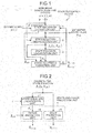
- FIG. 1 is a block diagram illustrating an outline of the overall configuration of a state estimation device according to this embodiment.
- a state estimation device 10 illustrated in FIG. 1 includes a state-and-error estimation unit 1, a state-equation discretization unit 2, a state-equation linearization unit 3, and a state-and-error prediction unit 4.
- the state estimation device uses a system noise covariance matrix Q and an observation noise covariance matrix R, both of which are design parameters.
- the state-and-error estimation unit 1 provides an estimated value x k
- the state-equation discretization unit 2 outputs a discrete-time state equation f d (t k , x k
- the state-equation linearization unit 3 calculates, from the discrete-time state equation f d (t k , x k
- the suffix T indicates a transposed matrix.
- FIG. 2 is a block diagram illustrating details of the state-and-error prediction unit 4 illustrated in FIG. 1 .
- the state-and-error prediction unit 4 illustrated in FIG. 2 includes a state prediction unit 5 and an error prediction unit 6.
- the state prediction unit 5 outputs the discrete-time state equation f d (t k , x k
- t t k
- x x k
- k (hat), and the system noise covariance matrix Q the error prediction unit 6 calculates a predicted value of the error covariance matrix ⁇ k+1
- FIG. 3 is a block diagram illustrating a hardware configuration of the state estimation device 10 illustrated in FIG. 1 .
- the state estimation device 10 illustrated in FIG. 3 includes a processor 21, a memory 22, and a system interface 23.
- the processor 21 performs state estimation.
- the memory 22 stores a program and data.
- the system interface 23 reads an output from the target system.
- the state estimation device 10 is connected to an input device 24 and a display device 25.
- the input device 24 receives inputs of initial values and design parameters.
- the display device 25 is an example of a unit for outputting an estimation result.
- the processor 21 executes a program stored in the memory 22 to calculate an estimated state value of the target system on the basis of: initial values and design parameters that are set via the input device 24; and an output value from the target system obtained via the system interface 23.
- the estimated state value output from the processor 21 is displayed on the display device 25.
- the processor 21 is, for example, a central processing unit (CPU).
- the memory 22 is, for example, a random access memory (RAM), a read-only memory (ROM), or a flash memory.
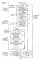
- FIG. 4 is a flowchart illustrating an operation of the state estimation device according to this embodiment.
- the nonlinear model of the target system can be expressed by the nonlinear state equation and the linear observation equation of Formula (1) below.
- the state value and the error covariance matrix value at the time t k estimated on the basis of the output value y(t k ) at the time t k are represented as x k
- the state value and the error covariance matrix value at a next time point t k+1 predicted on the basis of the output value y(t k ) at the time t k are represented as x k+1
- the state-and-error estimation unit 1 performs initialization (S1). Specifically, the state-and-error estimation unit 1 provides initial values that are a predicted state value x 1
- the state-and-error estimation unit 1 calculates a Kalman gain K k (S2). Specifically, the state-and-error estimation unit 1 calculates a Kalman gain K k by using below Formula (2) at the time t k , on the basis of: the predicted current error covariance matrix value ⁇ k
- k-1 (hat) is an n ⁇ n matrix
- R is a q ⁇ q matrix
- K k is an n ⁇ q matrix.
- the suffix "-1" indicates an inverse matrix.
- K k ⁇ ⁇ k
- the state-and-error estimation unit 1 calculates the estimated error covariance matrix value ⁇ k
- Formula (3) represents a difference between the predicted error covariance matrix value ⁇ k
- k (hat) is an n ⁇ n matrix. [Formula 3] ⁇ ⁇ k
- k ⁇ ⁇ k
- the state-and-error estimation unit 1 calculates the estimated state value x k
- Formula (4) represents a sum of the predicted state value x k
- k (hat) is an n ⁇ 1 matrix.
- the state x(t k+1 ) for the next time point is expressed by below Formula (5) representing a sum of the current state x(t k ) and an integral value of the state equation from the time t k to the time t k+1 .
- Formula (5) representing a sum of the current state x(t k ) and an integral value of the state equation from the time t k to the time t k+1 .
- the quadratic or higher-order numerical integration technique is, for example, a calculation technique using a fourth-order Runge-Kutta method as discussed below.
- the state-equation discretization unit 2 then substitutes x k
- the state prediction unit 5 calculates the predicted state value x k+1
- k f d t k x ⁇ k
- the state-equation linearization unit 3 calculates the approximate Jacobian value F k on the basis of the discrete-time state equation f d and a predetermined infinitesimal scalar value ⁇ by using a difference method. Note that F k is an n ⁇ n matrix.
- the state-equation linearization unit 3 first calculates a value x i (hat) (S8). Specifically, as shown by below Formula (7), the state-equation linearization unit 3 multiplies only the i-th component of the state by (1+ ⁇ ) with respect to the current estimated state value x k
- the state-equation linearization unit 3 then performs a calculation using a quadratic or higher-order numerical integration (S9), and calculates the i-th column of the Jacobian approximate value by using a difference method (S10). Specifically, the state-equation linearization unit 3 calculates the value of the discrete-time state equation on the basis of x i (hat) by using the above described numerical integration technique.
- the error prediction unit 6 calculates the predicted error covariance matrix value ⁇ k+1
- k F k ⁇ ⁇ k
- the state estimation device 10 then advances the time from t k to t k+1 , and thus repeats the above steps S2 to S11 to output the estimated state value at each time point.
- the calculation operations at the above steps are performed in the processor 21.
- the calculated values obtained at the corresponding steps such as the Kalman gain K k , the estimated values x k
- the state estimation device enables a high-order, i.e., quadratic or higher-order, integration technique to be applied to discretization of the state equation because an approximate Jacobian value is calculated on the basis of the estimated state value at each time point. This can reduce the discretization error in the process of state estimation that uses an extended Kalman filter, and can thus improve state estimation accuracy.
- One known state estimation device for a nonlinear system other than one that uses an extended Kalman filter is a state estimation device that uses an unscented Kalman filter.
- Use of an extended Kalman filter enables the state estimation device according to the present invention to reduce the number of design parameters requiring adjustment, and also reduce the amount of calculation as compared to when an unscented Kalman filter is used.
- the state estimation device of this embodiment uses a fourth-order Runge-Kutta method for the approximation relating to Formula (5) described above, but the present invention is not limited thereto.
- An integration technique having accuracy of quadratic or higher-order approximation, such as Heun's method, can be satisfactorily used.
- the infinitesimal scalar value ⁇ which the state-equation linearization unit 3 uses in a difference method is preferably as low a value as possible depending on the target system, and may be externally changeable via the input device 24 depending on an estimation result displayed on the display device 25. Externally changing the infinitesimal scalar value ⁇ to a minimum value without causing an anomaly such as divergence of an estimation result can reduce the error caused by approximation of the Jacobian.
- a matrix of vector n ⁇ 1 may be used as the parameter ⁇ , such that the calculation is performed using an infinitesimal value ⁇ (i) that is partially or wholly different across the states, as given by Formula (10) below.
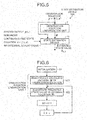
- FIG. 5 is a block diagram illustrating an outline of the overall configuration of a state estimation device according to this embodiment.
- a state estimation device 10A illustrated in FIG. 5 includes an observation-equation linearization unit 7 and the state estimation device 10 illustrated in FIG. 1 . Note that description of components and operations similar to those of the first embodiment will be omitted.
- the state estimation device 10A receives, as inputs, these equations and the system output y(t k ) at each time point, and uses the system noise covariance matrix Q and the observation noise covariance matrix R both of which are design parameters.
- the observation-equation linearization unit 7 analytically calculates a Jacobian H from the observation equation h(t, x). From the Jacobian H k of the observation equation, the system output y(t k ), the predicted current state value x k
- the state-equation discretization unit 2, the state-equation linearization unit 3, and the state-and-error prediction unit 4 operate similarly to the first embodiment.
- the operation of the state estimation device 10A illustrated in FIG. 6 further includes an operation of the observation-equation linearization unit 7 between step S1 and step S2 of the flowchart illustrated in FIG. 4 .
- the observation-equation linearization unit 7 substitutes, at each time point, the predicted state value x k
- k-1 (hat) is an n ⁇ 1 matrix
- H k is a q ⁇ n matrix.
- state estimation is performed by replacing the coefficient C of the observation equation in the first embodiment with the Jacobian H k , and by using the original nonlinear function h(t k , x k
- the calculation operations at the above steps are performed in the processor 21.
- the calculated values obtained at the corresponding steps such as the Kalman gain K k , the estimated values x k
- the state estimation device can reduce the amount of calculation by analytically calculating the Jacobian of the observation equation that needs no discretization. Further, the state estimation device according to this embodiment enables a high-order, i.e., quadratic or higher-order, integration technique to be applied to discretization of the state equation because an approximate value of the Jacobian of the state equation is calculated on the basis of the estimated state value at each time point. As a result, it becomes possible to reduce the discretization error in the process of state estimation that uses an extended Kalman filter, and thus improve state estimation accuracy.
- FIG. 7 is a block diagram illustrating an outline of the overall configuration of a state estimation device according to this embodiment.
- a state estimation device 10B illustrated in FIG. 7 includes the observation-equation linearization unit 7, the state-and-error estimation unit 1, the state-equation discretization unit 2, the state-equation linearization unit 3, the state prediction unit 5, and the error prediction unit 6. Note that description of components and operations similar to those of the first and second embodiments will be omitted.
- the hardware configuration is that which is discussed with reference to FIG. 3
- the flowchart is that which is discussed with reference to FIG. 6 .
- the state estimation device uses design parameters: the system noise covariance matrix Q; the observation noise covariance matrix R; and the infinitesimal scalar value ⁇ to be used in a difference method.
- the observation-equation linearization unit 7 analytically calculates the Jacobian H from the observation equation h(t, x, u). From the Jacobian H k of the observation equation, system output y(t k ), the predicted current state value x k
- the state-equation discretization unit 2 outputs a discrete-time state equation f d (t k , x k
- k (hat), u(t k )), which has been discretized using a fourth-order Runge-Kutta method, on the basis of: the nonlinear continuous-time state equation (d/dt)x f(t, x, u); the current state and error covariance matrix x k
- the state-equation linearization unit 3 calculates the Jacobian ⁇ f d (t, x, u)/ ⁇ x T
- k (hat), u u(t k ) of the state equation by using a difference method.
- the state prediction unit 5 outputs the discretization-time state equation f d (t k , x k
- the error prediction unit 6 calculates the predicted error covariance matrix value ⁇ k+1
- the initialization operation at step S1 is similar to the initialization operation in the first embodiment.
- the observation-equation linearization unit 7 substitutes, at each time point, the predicted state value x k
- k-1 (hat) is an n ⁇ 1 matrix
- H k is a q ⁇ n matrix.
- the state-and-error estimation unit 1 calculates the Kalman gain K k from: the predicted current error covariance matrix value ⁇ k
- K k ⁇ ⁇ k
- the state-and-error estimation unit 1 calculates the current estimated error covariance matrix value ⁇ k
- k (hat) is the difference between the predicted error covariance matrix value ⁇ k
- k (hat) is an n ⁇ n matrix. [Formula 20] ⁇ ⁇ k
- k ⁇ ⁇ k
- the state-and-error estimation unit 1 calculates the current estimated state value x k
- k (hat) is a sum of the predicted current state value x k
- k (hat) is an n ⁇ 1 matrix.
- the state x(t k+1 ) for the next time point is expressed by a sum of the current state x(t k ) and an integral value of the state equation from the time t k to the time t k+1 , as shown by below Formula (22).
- the quadratic or higher-order numerical integration technique is, for example, a calculation technique using a fourth-order Runge-Kutta method that also takes into account the system input.
- x t k + 1 x t k + ⁇ t k t k + 1 f t , x t , u t dt
- ⁇ f(t k +( ⁇ T/2), ⁇ ,, u(t k )) is calculated using the result of calculation of this ⁇ .
- ⁇ f(t k+1 , ⁇ , u(t k )) is calculated using the result of calculation of this ⁇ .
- the state-equation discretization unit 2 then substitutes the current estimated state value x k
- the state prediction unit 5 outputs the discrete-time state equation f d (t k , x k
- k f d t k , x ⁇ k
- the state-equation linearization unit 3 calculates the approximate Jacobian value F k on the basis of the discrete-time state equation f d (t k , x k
- the state-equation linearization unit 3 first calculates x i (hat) from the current estimated state value x k
- the error prediction unit 6 calculates the error covariance matrix ⁇ k+1
- Q is an n ⁇ n matrix.
- the calculation operations at the above steps are performed in the processor 21.
- the calculated values obtained at the corresponding steps such as the Kalman gain K k , the estimated values x k
- the state estimation device enables a high-order, i.e., quadratic or higher-order, integration technique to be applied to discretization of the state equation because an approximate Jacobian value is calculated on the basis of the estimated state value at each time point. This can reduce the discretization error in the process of state estimation that uses an extended Kalman filter, and can thus improve state estimation accuracy.
- the state estimation device uses a fourth-order Runge-Kutta method for the approximation relating to Formula (22) described above, but the present invention is not limited thereto.
- An integration technique having accuracy of quadratic or higher-order approximation, such as Heun's method, can be satisfactorily used.
- the present invention is also applicable to a case in which the observation equation is a linear function.
- the case in which the observation equation is a linear function can be addressed by omitting the observation-equation linearization unit 7, and using H k that is the coefficient matrix for the state in the observation equation.
- the infinitesimal scalar value ⁇ used in a difference method is preferably as low a value as possible depending on the target system, and may be externally changeable via the input device 24 depending on an estimation result displayed on the display device 25. Externally changing the infinitesimal scalar value ⁇ to a minimum value without causing an anomaly such as divergence of the estimation result can reduce the error caused by approximation of the Jacobian.
- a matrix of vector n ⁇ 1 may be used as the parameter ⁇ , such that the calculation is performed using an infinitesimal value ⁇ (i) that is partially or wholly different across the states, as given by Formula (26) below.
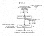
- FIG. 8 is a block diagram illustrating an outline of the overall configuration of a state estimation device according to this embodiment.
- a state estimation device 10C illustrated in FIG. 8 includes a model conversion unit 8 and the state estimation device 10B illustrated in FIG. 7 . Note that description of components and operations similar to those of the first to third embodiments will be omitted.
- the hardware configuration is that which is discussed with reference to FIG. 3
- the flowchart is that which is discussed with reference to FIG. 4 .
- the state estimation device 10C uses design parameters: the system noise covariance matrix Q; the observation noise covariance matrix R; and the infinitesimal scalar value ⁇ to be used in a difference method.
- the state estimation device 10C estimates the unknown parameter ⁇ and the state x at the same time.
- the model conversion unit 8 converts the continuous-time models into respective nonlinear continuous-time models using a new state vector having therein the state x and the unknown parameter ⁇ before conversion.
- the state estimation device 10B uses, as inputs, the nonlinear continuous-time model generated by the conversion, and calculates an estimated value of the new state vector.
- the observation-equation linearization unit 7, the state-and-error estimation unit 1, the state-equation discretization unit 2, the state-equation linearization unit 3, the state prediction unit 5, and the error prediction unit 6 of the state estimation device 10B are identical to those of the first to third embodiments.
- the process includes an additional operation to be performed by the model conversion unit 8 before the initialization step (S1) in FIG. 4 or FIG. 6 .
- x (tilde) is an (n+p) ⁇ 1 matrix.
- the unknown parameter ⁇ in a case in which the unknown parameter ⁇ varies in time, the unknown parameter ⁇ is modeled, and is set as n+1:n+p components of the function f (tilde).
- the n+1:n+p components of the function f (tilde) are set to zero.
- the subsequent operations are similar to those shown in FIG. 4 , and the estimated value of the new vector x (tilde) is calculated using Formula (30) below. [Formula 30] x ⁇ ⁇ k
- k x ⁇ k
- the calculation operations at the above steps are performed in the processor 21.
- the calculated values obtained at the corresponding steps such as the Kalman gain K k , the estimated values x k
- the state estimation device can estimate the state by conversion of the continuous-time model into a model having a new state having therein the state and the unknown parameter before conversion. This can reduce the discretization error, and can thus perform state estimation and parameter estimation with high accuracy.
- the continuous-time model containing an unknown parameter, used as inputs in this embodiment may be nonlinear or linear, and even linear continuous-time model is output as a nonlinear model from the model conversion unit.
- the continuous-time model causes the model conversion unit to provide an output that includes a nonlinear continuous-time state equation
- the unknown parameter may be contained in one or both of the state equation and the observation equation.
- the continuous-time models may or may not contain a system input.
- 1 state-and-error estimation unit 2 state-equation discretization unit; 3 state-equation linearization unit; 4 state-and-error prediction unit; 5 state prediction unit; 6 error prediction unit; 7 observation-equation linearization unit; 8 model conversion unit; 10, 10A, 10B, 10C state estimation device; 21 processor; 22 memory; 23 system interface; 24 input device; 25 display device.
Landscapes
- Engineering & Computer Science (AREA)
- Physics & Mathematics (AREA)
- General Physics & Mathematics (AREA)
- Software Systems (AREA)
- Health & Medical Sciences (AREA)
- Artificial Intelligence (AREA)
- Computer Vision & Pattern Recognition (AREA)
- Evolutionary Computation (AREA)
- Medical Informatics (AREA)
- Automation & Control Theory (AREA)
- Computational Mathematics (AREA)
- Mathematical Analysis (AREA)
- Mathematical Optimization (AREA)
- Pure & Applied Mathematics (AREA)
- Data Mining & Analysis (AREA)
- Mathematical Physics (AREA)
- Theoretical Computer Science (AREA)
- Algebra (AREA)
- Databases & Information Systems (AREA)
- General Engineering & Computer Science (AREA)
- Management, Administration, Business Operations System, And Electronic Commerce (AREA)
- Complex Calculations (AREA)
Abstract
Description
- The present invention relates to a state estimation device that estimates a state or parameter of a target system.
- As one example of a conventional state estimation device for a nonlinear system, Non-Patent Literature 1 discloses a state estimation device that uses an extended Kalman filter (EKF). Extended Kalman filter is used for estimation of an internal state of a system on the basis of both an output from a target system and a nonlinear discrete-time system that is the modeled target system. In addition, when that system has an unknown parameter, the system is converted into an expanded system containing the unknown parameter as a state, and an extended Kalman filter is then applied thereto to estimate the state and the parameter. For such extended Kalman filter to be applied to a nonlinear system, the system is linearized using first-order Taylor approximation, which requires the Jacobian of a state equation or observation equation. Moreover, as the target system is a nonlinear discrete-time system, the state equation should be discretized beforehand if the state equation is given in continuous time.
- For example,
Patent Literature 1 discloses a technology that, where the target system is represented as a nonlinear continuous-time system, discretizes the target system beforehand by using an Euler method, and then applies an extended Kalman filter to thereby estimate the state and an unknown parameter. - In other words, where the target system is the nonlinear discrete-time system and the state equation is given in continuous time, the use of an extended Kalman filter requires the discretization. The process for estimating the state by using an extended Kalman filter needs calculation of the Jacobian of the state equation.
- Patent Literature 1: Japanese Patent Application Laid-open No.
2005-248946 - Non-Patent Literature 1: Takashi YAHAGI, "Kalman Filter and Adaptive Signal Processing", Corona publishing, Dec. 2005, pp.48-51
- Unfortunately, the conventional technology described above has difficulties in calculating a Jacobian in a case in which a quadratic or higher-order discretization technique is used for discretization of a continuous-time state equation. To address this issue, the discretization needs to be performed using an Euler method that can analytically derive a Jacobian. However, such an Euler method, which provides accuracy of first-order approximation, poses a problem of only conducting the estimation with low accuracy due to a large discretization error in a case in which the target is formulated by a continuous-time state equation.
- The present invention has been made in view of the foregoing, and it is an object of the present invention to provide a state estimation device capable of estimating a state with high accuracy by using an extended Kalman filter in a case in which the state equation of a target system is a nonlinear continuous-time function.
- To solve the above problem and achieve the object, the present invention provides a state estimation device to receive, as inputs, an output from a target system and a nonlinear model for estimating a state of the target system by using an extended Kalman filter, the nonlinear model being a modeled target system, wherein the nonlinear model includes a nonlinear continuous-time state equation, the state estimation device comprising: a state-and-error estimation unit to, on a basis of an observation equation of the nonlinear model, obtain an estimated state value and an estimated value of an error covariance matrix of the estimated state value, the estimated state value estimating a state of the target system at a certain time point; a state-equation discretization unit to obtain a discrete-time state equation by discretizing the nonlinear continuous-time state equation on the basis of the estimated state value at the time point, by using a quadratic or higher-order integration technique; a state-equation linearization unit to obtain an approximate value of a Jacobian at the time point by using the discrete-time state equation at the time point and a difference method; and a state-and-error prediction unit to predict, from the approximate value of the Jacobian, the error covariance matrix provided after a lapse of an infinitesimal time period since the time point, and to predict, from the discrete-time state equation, the state provided after a lapse of the infinitesimal time period since the time point.
- The state estimation device according to the present invention is capable of estimating the state with the high accuracy by using an extended Kalman filter in a case in which the state equation of the target system is the nonlinear continuous-time function.
-
-
FIG. 1 is a block diagram illustrating an outline of the overall configuration of a state estimation device according to a first embodiment. -
FIG. 2 is a block diagram illustrating details of the state-and-error prediction unit illustrated inFIG. 1 . -
FIG. 3 is a block diagram illustrating a hardware configuration of the state estimation device illustrated inFIG. 1 . -
FIG. 4 is a flowchart illustrating an operation of the state estimation device according to the first embodiment. -
FIG. 5 is a block diagram illustrating an outline of the overall configuration of a state estimation device according to a second embodiment. -
FIG. 6 is a flowchart illustrating an operation of the state estimation device according to the second embodiment. -
FIG. 7 is a block diagram illustrating an outline of the overall configuration of a state estimation device according to a third embodiment. -
FIG. 8 is a block diagram illustrating an outline of the overall configuration of a state estimation device according to a fourth embodiment. - A state estimation device according to embodiments of the present invention will be described in detail below with reference to the drawings. Note that these embodiments are not intended to limit the scope of this invention.
- Note that, in the description below, the parameters are vector values except for the time t and the scalar value ε. However, no particular distinction is made therebetween in the specification, but a vector value is indicated in bold in a mathematical formula. In addition, temporal differentiation is expressed as (d/dt)x in the specification, but is indicated by a dot above the applicable letter in a mathematical formula. Furthermore, a predicted value and an estimated value are indicated by a notation of "(hat)" in the specification, but by a hat symbol above the applicable letter in a mathematical formula. A state value or an equation of an expanded system model is indicated by a notation of "(tilde)", but by a tilde above the applicable letter in a mathematical formula.
-
FIG. 1 is a block diagram illustrating an outline of the overall configuration of a state estimation device according to this embodiment. Astate estimation device 10 illustrated inFIG. 1 includes a state-and-error estimation unit 1, a state-equation discretization unit 2, a state-equation linearization unit 3, and a state-and-error prediction unit 4. The state estimation device according to this embodiment receives, as inputs, a target-system nonlinear continuous-time state equation (d/dt)x=f(t, x), a linear observation equation y=Cx, and a system output y(tk) at each time point. The state estimation device uses a system noise covariance matrix Q and an observation noise covariance matrix R, both of which are design parameters. - The state-and-
error estimation unit 1 provides an estimated value xk|k (hat) of a current state and an estimated value ∑k|k (hat) of a current error covariance matrix, on the basis of: a coefficient C of the linear observation equation; the system output y(tk) at a current time tk; the observation noise covariance matrix R; and a predicted current state value xk|k-1 (hat) and a predicted current error covariance matrix value ∑k|k-1 (hat) both of which were calculated at a previous time point. - The state-
equation discretization unit 2 outputs a discrete-time state equation fd(tk, xk|k (hat)), which has been discretized using a fourth-order Runge-Kutta method, on the basis of the nonlinear continuous-time state equation f(t, x) and the current estimated state value xk|k (hat). - The state-
equation linearization unit 3 calculates, from the discrete-time state equation fd(tk, xk|k (hat)), an approximate value of the Jacobian ∂fd(t, x)/∂xT|t=tk, x=xk|k (hat) of the state equation by using a difference method. Note that the suffix T indicates a transposed matrix. -
FIG. 2 is a block diagram illustrating details of the state-and-error prediction unit 4 illustrated inFIG. 1 . The state-and-error prediction unit 4 illustrated inFIG. 2 includes astate prediction unit 5 and anerror prediction unit 6. - The
state prediction unit 5 outputs the discrete-time state equation fd(tk, xk|k (hat)) as the predicted state value xk+1|k (hat) for a next time point. From ∂fd(t, x)/∂xT|t=tk, x=xk|k (hat) (i.e., the Jacobian Fk of the state equation), the estimated current error covariance matrix value ∑k|k (hat), and the system noise covariance matrix Q, theerror prediction unit 6 calculates a predicted value of the error covariance matrix ∑k+1|k (hat) for the next time point. -
FIG. 3 is a block diagram illustrating a hardware configuration of thestate estimation device 10 illustrated inFIG. 1 . Thestate estimation device 10 illustrated inFIG. 3 includes aprocessor 21, a memory 22, and asystem interface 23. Theprocessor 21 performs state estimation. The memory 22 stores a program and data. Thesystem interface 23 reads an output from the target system. Thestate estimation device 10 is connected to aninput device 24 and a display device 25. Theinput device 24 receives inputs of initial values and design parameters. The display device 25 is an example of a unit for outputting an estimation result. Theprocessor 21 executes a program stored in the memory 22 to calculate an estimated state value of the target system on the basis of: initial values and design parameters that are set via theinput device 24; and an output value from the target system obtained via thesystem interface 23. The estimated state value output from theprocessor 21 is displayed on the display device 25. Theprocessor 21 is, for example, a central processing unit (CPU). The memory 22 is, for example, a random access memory (RAM), a read-only memory (ROM), or a flash memory. -
FIG. 4 is a flowchart illustrating an operation of the state estimation device according to this embodiment. Assume that the nonlinear model of the target system can be expressed by the nonlinear state equation and the linear observation equation of Formula (1) below.
[Formula 1]
- In addition, the state value and the error covariance matrix value at the time tk estimated on the basis of the output value y(tk) at the time tk are represented as xk|k (hat) and ∑k|k (hat), respectively. The state value and the error covariance matrix value at a next time point tk+1 predicted on the basis of the output value y(tk) at the time tk are represented as xk+1|k (hat) and ∑k+1|k (hat), respectively.
- First, the state-and-
error estimation unit 1 performs initialization (S1). Specifically, the state-and-error estimation unit 1 provides initial values that are a predicted state value x1|0 (hat) and a predicted error covariance matrix value ∑1|0 (hat) at a state estimation start time t1. - Next, the state-and-
error estimation unit 1 calculates a Kalman gain Kk (S2). Specifically, the state-and-error estimation unit 1 calculates a Kalman gain Kk by using below Formula (2) at the time tk, on the basis of: the predicted current error covariance matrix value ∑k|k-1 (hat) calculated at a previous time point tk-1; the coefficient C of the linear observation equation; and the observation noise covariance matrix R. Note here that ∑k|k-1 (hat) is an n×n matrix, R is a q×q matrix, and Kk is an n×q matrix. Note that the suffix "-1" indicates an inverse matrix.
[Formula 2]
- Next, the state-and-
error estimation unit 1 calculates the estimated error covariance matrix value ∑k|k (hat) (S3). Specifically, the state-and-error estimation unit 1 calculates the current estimated error covariance matrix value ∑k|k (hat) by using below Formula (3). Formula (3) represents a difference between the predicted error covariance matrix value ∑k|k-1 (hat) and a matrix that is a product obtained by multiplying this predicted value ∑k|k-1 (hat) by both the Kalman gain Kk and the coefficient C of the linear observation equation. Note that ∑k|k (hat) is an n×n matrix.
[Formula 3]
- Then, the state-and-
error estimation unit 1 calculates the estimated state value xk|k (hat) (S4). Specifically, the state-and-error estimation unit 1 calculates the current estimated state value xk|k (hat) by using below Formula (4). Formula (4) represents a sum of the predicted state value xk|k-1 (hat) and a value that is obtained by multiplying a difference by the Kalman gain Kk, the difference being obtained by subtracting, from the current system output y(tk), the system output yk|k-1 (hat) predicted using the linear observation equation. Note that xk|k (hat) is an n×1 matrix.
[Formula 4]
- In the state-
equation discretization unit 2, the state x(tk+1) for the next time point is expressed by below Formula (5) representing a sum of the current state x(tk) and an integral value of the state equation from the time tk to the time tk+1.
[Formula 5]
- Therefore, the state
equation discretization unit 2 calculates an approximate value of the nonlinear discrete-time state equation x(tk+1) = fd(tk, x(tk)) by using a quadratic or higher-order integration technique. The quadratic or higher-order numerical integration technique is, for example, a calculation technique using a fourth-order Runge-Kutta method as discussed below. - First, α=f(tk, x(tk)) is calculated from the current state x(tk).
- Next, β=x(tk)+(ΔT/2)α is calculated using the result of calculation of this α and a time interval ΔT=tk+1-tk.
- Then, γ=f(tk+(ΔT/2), β) is calculated using the result of calculation of this β.
- Then, λ=x(tk) + (ΔT/2)γ is calculated using the result of calculation of this γ.
- Then, ζ=f(tk+(ΔT/2), λ) is calculated using the result of calculation of this λ.
- Then, η=x(tk)+ΔTζ is calculated using the result of calculation of this ζ.
- Then, ξ=f(tk+1, η) is calculated using the result of calculation of this η.
- Then, the discrete-time state equation fd(tk, x(tk)) = x(tk) + (ΔT/6) (α+2(γ+ζ)+ξ) is calculated.
- The state-
equation discretization unit 2 then substitutes xk|k (hat) for x(tk) (S5), and performs a calculation using a quadratic or higher-order numerical integration technique (S6). Specifically, the state-equation discretization unit 2 substitutes the current estimated state value xk|k (hat) for the current state x(tk), and calculates the discrete-time state equation fd(tk, xk|k (hat)) by using the above Runge-Kutta method. - The
state prediction unit 5 calculates the predicted state value xk+1|k (hat) (S7). Specifically, as shown by below Formula (6), thestate prediction unit 5 outputs the value of the discrete-time state equation fd(tk, xk|k (hat)) as the predicted state value xk+1|k (hat) for the next time point tk+1.
[Formula 6]
- The state-
equation linearization unit 3 calculates the approximate Jacobian value Fk on the basis of the discrete-time state equation fd and a predetermined infinitesimal scalar value ε by using a difference method. Note that Fk is an n×n matrix. The state-equation linearization unit 3 first calculates a value xi (hat) (S8). Specifically, as shown by below Formula (7), the state-equation linearization unit 3 multiplies only the i-th component of the state by (1+ε) with respect to the current estimated state value xk|k (hat), thereby providing the resulting value xi (hat).
[Formula 7]

n × n matrix having (i, i) elements being 1, and the other elements being 0 - The state-
equation linearization unit 3 then performs a calculation using a quadratic or higher-order numerical integration (S9), and calculates the i-th column of the Jacobian approximate value by using a difference method (S10). Specifically, the state-equation linearization unit 3 calculates the value of the discrete-time state equation on the basis of xi (hat) by using the above described numerical integration technique. Then, as shown by below Formula (8), the state-equation linearization unit 3 approximates the i-th column (i=1, 2, ..., n) of the Jacobian by providing a value obtained by dividing, by a value εxk|k(i) (hat), the difference from the discrete-time state equation fd(tk, xk|k (hat)) for the current estimated state value xk|k (hat), the value εxk|k(i) (hat) being obtained by multiplying the i-th component of the current estimated state value by ε. Note that this operation is consecutively repeated from i=1 to i=n.
[Formula 8]
- Then, the
error prediction unit 6 calculates the predicted error covariance matrix value ∑k+1|k (hat) (S11). Specifically, theerror prediction unit 6 calculates the error covariance matrix ∑k+1|k (hat) for the next time point on the basis of: the approximate Jacobian value Fk; the current estimated error covariance matrix value ∑k|k (hat); and the system noise covariance matrix Q, by using Formula (9) below. Note that Q is an n×n matrix.
[Formula 9]
- The
state estimation device 10 then advances the time from tk to tk+1, and thus repeats the above steps S2 to S11 to output the estimated state value at each time point. The calculation operations at the above steps are performed in theprocessor 21. The calculated values obtained at the corresponding steps, such as the Kalman gain Kk, the estimated values xk|k (hat) and ∑k|k (hat), the predicted values xk|k-1 (hat) and ∑k|k-1 (hat), the discrete-time state equation fd, and the approximate Jacobian value Fk of the state equation are stored in the memory 22 and are read from the memory 22 and used at the corresponding steps. - As described above, even when the state equation of a target system is given by a nonlinear continuous-time function, the state estimation device according to this embodiment enables a high-order, i.e., quadratic or higher-order, integration technique to be applied to discretization of the state equation because an approximate Jacobian value is calculated on the basis of the estimated state value at each time point. This can reduce the discretization error in the process of state estimation that uses an extended Kalman filter, and can thus improve state estimation accuracy.
- One known state estimation device for a nonlinear system other than one that uses an extended Kalman filter is a state estimation device that uses an unscented Kalman filter. Use of an extended Kalman filter enables the state estimation device according to the present invention to reduce the number of design parameters requiring adjustment, and also reduce the amount of calculation as compared to when an unscented Kalman filter is used. Note that the state estimation device of this embodiment uses a fourth-order Runge-Kutta method for the approximation relating to Formula (5) described above, but the present invention is not limited thereto. An integration technique having accuracy of quadratic or higher-order approximation, such as Heun's method, can be satisfactorily used.
- The infinitesimal scalar value ε which the state-
equation linearization unit 3 uses in a difference method is preferably as low a value as possible depending on the target system, and may be externally changeable via theinput device 24 depending on an estimation result displayed on the display device 25. Externally changing the infinitesimal scalar value ε to a minimum value without causing an anomaly such as divergence of an estimation result can reduce the error caused by approximation of the Jacobian. In addition, instead of using an infinitesimal scalar value ε, a matrix of vector n×1 may be used as the parameter ε, such that the calculation is performed using an infinitesimal value ε(i) that is partially or wholly different across the states, as given by Formula (10) below.
[Formula 10]
- Moreover, if a relationship of xk|k(i) (hat)≈0 applies, Formula (11) below may be used instead, which uses an infinitesimal value ε' temporarily or for the entire period.
[Formula 11]

n-dimensional vector having an i-th component being 1, and the other elements being 0 -
FIG. 5 is a block diagram illustrating an outline of the overall configuration of a state estimation device according to this embodiment. Astate estimation device 10A illustrated inFIG. 5 includes an observation-equation linearization unit 7 and thestate estimation device 10 illustrated inFIG. 1 . Note that description of components and operations similar to those of the first embodiment will be omitted. For the state estimation device according to this embodiment, a target system is represented by the nonlinear continuous-time state equation (d/dt)x=f(t, x) and a nonlinear observation equation y=h(t, x). Thestate estimation device 10A receives, as inputs, these equations and the system output y(tk) at each time point, and uses the system noise covariance matrix Q and the observation noise covariance matrix R both of which are design parameters. The nonlinear observation equation y=h(t, x) is used in place of the linear observation equation y=Cx. - The observation-
equation linearization unit 7 analytically calculates a Jacobian H from the observation equation h(t, x). From the Jacobian Hk of the observation equation, the system output y(tk), the predicted current state value xk|k-1 (hat), and ∑k|k-1 (hat), the state-and-error estimation unit 1 provides the current estimated value xk|k (hat) of the state and the current estimated valus ∑k|k (hat) of the error covariance matrix. The state-equation discretization unit 2, the state-equation linearization unit 3, and the state-and-error prediction unit 4 operate similarly to the first embodiment. -
FIG. 6 is a flowchart illustrating an operation of the state estimation device according to this embodiment. Steps S1 and S2 to S11 of the flowchart ofFIG. 6 are those which are discussed with reference toFIG. 4 . Note that this mention of steps S2 to S11 includes the operations of i=1 and i++. Assume that the nonlinear model of the target system can be expressed by the nonlinear continuous-time state equation and the nonlinear observation equation of Formula (12) below.
[Formula 12]
- The operation of the
state estimation device 10A illustrated inFIG. 6 further includes an operation of the observation-equation linearization unit 7 between step S1 and step S2 of the flowchart illustrated inFIG. 4 . The observation-equation linearization unit 7 analytically calculates the Jacobian H of the observation equation, as shown by below Formula (13) (S21). Note that H is a q×n matrix.
[Formula 13]
- Next, the observation-
equation linearization unit 7 substitutes, at each time point, the predicted state value xk|k-1 (hat) for the current time tk in the Jacobian of the observation equation as shown by below Formula (14), and thus obtains the current Jacobian Hk of the observation equation (S22). Note that xk|k-1 (hat) is an n×1 matrix, and Hk is a q×n matrix.
[Formula 14]
- From Formula (14), the observation equation can be approximated by a product obtained by multiplying the state by the Jacobian in a vicinity of the predicted current state value xk|k-1 (hat), as shown by below Formula (15) .
[Formula 15]
- Thus, state estimation is performed by replacing the coefficient C of the observation equation in the first embodiment with the Jacobian Hk, and by using the original nonlinear function h(tk, xk|k-1 (hat)) for the purpose of calculation of the predicted output value yk|k-1 (hat). The calculation operations at the above steps are performed in the
processor 21. The calculated values obtained at the corresponding steps, such as the Kalman gain Kk, the estimated values xk|k (hat) and ∑k|k (hat), the predicted values xk|k-1 (hat) and ∑k|k-1. (hat), the discrete-time state equation fd, and the approximate Jacobian value Fk of the state equation are stored in the memory 22, and are read from the memory 22 and used at the corresponding steps. - As described above, even when the state equation of a target system is a nonlinear continuous-time function, and the observation equation is given by a nonlinear function, the state estimation device according to this embodiment can reduce the amount of calculation by analytically calculating the Jacobian of the observation equation that needs no discretization. Further, the state estimation device according to this embodiment enables a high-order, i.e., quadratic or higher-order, integration technique to be applied to discretization of the state equation because an approximate value of the Jacobian of the state equation is calculated on the basis of the estimated state value at each time point. As a result, it becomes possible to reduce the discretization error in the process of state estimation that uses an extended Kalman filter, and thus improve state estimation accuracy.
-
FIG. 7 is a block diagram illustrating an outline of the overall configuration of a state estimation device according to this embodiment. Astate estimation device 10B illustrated inFIG. 7 includes the observation-equation linearization unit 7, the state-and-error estimation unit 1, the state-equation discretization unit 2, the state-equation linearization unit 3, thestate prediction unit 5, and theerror prediction unit 6. Note that description of components and operations similar to those of the first and second embodiments will be omitted. The hardware configuration is that which is discussed with reference toFIG. 3 , and the flowchart is that which is discussed with reference toFIG. 6 . - The state estimation device according to this embodiment receives, as inputs, a target-system nonlinear continuous-time state equation (d/dt)x=f(t, x, u), an observation equation y=h(t, x, u), and system input and output u(tk) and y(tk) at each time point. The state estimation device according to this embodiment uses design parameters: the system noise covariance matrix Q; the observation noise covariance matrix R; and the infinitesimal scalar value ε to be used in a difference method. The nonlinear observation equation y=h(t, x, u) is used in place of the linear observation equation y=Cx.
- The observation-
equation linearization unit 7 analytically calculates the Jacobian H from the observation equation h(t, x, u). From the Jacobian Hk of the observation equation, system output y(tk), the predicted current state value xk|k-1 (hat), and the predicted current error covariance matrix value ∑k|k-1 (hat), the state-and-error estimation unit 1 provides the current estimated value xk|k (hat) of the state and the current estimated value ∑k|k (hat) of the error covariance matrix. - The state-
equation discretization unit 2 outputs a discrete-time state equation fd(tk, xk|k (hat), u(tk)), which has been discretized using a fourth-order Runge-Kutta method, on the basis of: the nonlinear continuous-time state equation (d/dt)x=f(t, x, u); the current state and error covariance matrix xk|k (hat) and ∑k|k (hat); and the system input u(tk). - From the discretization-time state equation fd(tk, xk|k (hat), u(tk)) and the infinitesimal scalar value ε, the state-
equation linearization unit 3 calculates the Jacobian ∂ fd(t, x, u)/∂xT|t=tk, x=xk|k (hat), u=u(tk) of the state equation by using a difference method. Thestate prediction unit 5 outputs the discretization-time state equation fd (tk, xk|k (hat), u(tk)) as the predicted state value xk+1|k (hat) for the next time point. From the Jacobian ∂fd(t, x, u)/∂xT|t=tk, x=xk|k (hat), u=u(tk) of the state equation, the current estimated error covariance matrix value ∑k|k (hat), and the system noise covariance matrix Q, theerror prediction unit 6 calculates the predicted error covariance matrix value ∑k+1|k (hat) for the next time point. - The state estimation device according to this embodiment will next be described in detail. First, assume that the nonlinear model of the target system can be expressed by the state equation and the observation equation of below Formula (16).
[Formula 16]
- The initialization operation at step S1 is similar to the initialization operation in the first embodiment. The observation-
equation linearization unit 7 analytically calculates the Jacobian H of the observation equation, as shown by below Formula (17) (S21). Note that H is a q×n matrix.
[Formula 17]
- Next, the observation-
equation linearization unit 7 substitutes, at each time point, the predicted state value xk|k-1 (hat) and the system input u(tk) for the current time tk into the Jacobian of the observation equation, and thus obtains the current Jacobian Hk as shown by below Formula (18) (S22). Note that xk|k-1 (hat) is an n×1 matrix, and Hk is a q×n matrix.
[Formula 18]
- Then, as shown by below Formula (19), the state-and-
error estimation unit 1 calculates the Kalman gain Kk from: the predicted current error covariance matrix value ∑k|k-1 (hat); the Jacobian Hk; and the observation noise covariance matrix R (S2).
[Formula 19]
- Next, the state-and-
error estimation unit 1 calculates the current estimated error covariance matrix value ∑k|k (hat) as shown by below Formula (20) (S3). The the current estimated error covariance matrix value ∑k|k (hat) is the difference between the predicted error covariance matrix value ∑k|k-1 (hat) and a matrix that is a product obtained by multiplying the predicted value ∑k|k-1 (hat) by both the Kalman gain Kk and the coefficient Hk of the observation equation. Note that ∑k|k (hat) is an n×n matrix.
[Formula 20]
- Then, the state-and-
error estimation unit 1 calculates the current estimated state value xk|k (hat) as shown by below Formula (21) (S4). The current estimated state value xk|k (hat) is a sum of the predicted current state value xk|k-1 (hat) and a product of the Kalman gain and a difference between the current system output y(tk) and the system output yk|k-1 (hat) that is predicted using the observation equation on the basis of the predicted state value xk|k-1 (hat) and the system input u(tk). Note that xk|k (hat) is an n×1 matrix.
[Formula 21]
- In the state-
equation discretization unit 2, the state x(tk+1) for the next time point is expressed by a sum of the current state x(tk) and an integral value of the state equation from the time tk to the time tk+1, as shown by below Formula (22). Thus, the state-equation discretization unit 2 calculates an approximate value of the nonlinear discrete-time state equation x(tk+1)=fd(tk, x(tk), u(tk)) by using a quadratic or higher-order integration technique. The quadratic or higher-order numerical integration technique is, for example, a calculation technique using a fourth-order Runge-Kutta method that also takes into account the system input.
[Formula 22]
- First, α=f(tk, x(tk), u(tk)) is calculated from the current state x(tk) and the system input u(tk).
- Next, β=x(tk)+(ΔT/2)α is calculated using the result of calculation of this α and a time interval ΔT=tk+1-tk.
- Then, γ=f(tk+(ΔT/2), β,, u(tk)) is calculated using the result of calculation of this β.
- Then, λ=x(tk)+(ΔT/2)γ is calculated using the result of calculation of this γ.
- Then, ζ=f(tk+(ΔT/2), λ, u(tk)) is calculated using the result of calculation of this λ.
- Then, η=x(tk)+ΔTζ is calculated using the result of calculation of this ζ.
- Then, ξ=f(tk+1, η, u(tk)) is calculated using the result of calculation of this η.
- Then, the discrete-time state equation fd(tk, x(tk), u(tk))=x(tk)+(ΔT/6) (α+2(γ+ζ)+ξ) is calculated.
- The state-
equation discretization unit 2 then substitutes the current estimated state value xk|k (hat) for the current state x(tk) (S5), and calculates the discrete-time state equation fd(tk, xk|k (hat), u(tk)) by using the above Runge-Kutta method (S6). - As shown by below Formula (23), the
state prediction unit 5 outputs the discrete-time state equation fd(tk, xk|k (hat), u(tk)) as the predicted state value ×k+1|k (hat) for the next time point tk+1 (S7).
[Formula 23]
- The state-
equation linearization unit 3 calculates the approximate Jacobian value Fk on the basis of the discrete-time state equation fd(tk, xk|k (hat), u(tk)) and the predetermined infinitesimal scalar value ε, by using a difference method. Note that Fk is an n×n matrix. The state-equation linearization unit 3 first calculates xi (hat) from the current estimated state value xk|k (hat), as shown by above Formula (7) (S8). - Next, the state-
equation linearization unit 3 calculates the value of the discrete-time state equation on the basis of xi (hat) by using the numerical integration technique described above (S9). Then, as shown by below Formula (24), the state-equation linearization unit 3 approximates the i-th column (i=1, 2, ..., n) of the Jacobian (S10) by providing a value obtained by dividing, by a value εxk|k(i) (hat), the difference from the discrete-time state equation fd(tk, xk|k (hat), u(tk)) for the current estimated state value xk|k (hat), the value εxk|k(i) (hat) being obtained by multiplying the i-th component of the current estimated state value by ε.
[Formula 24]

n × n matrix having (i, i) elements being 1, and the other elements being 0 - The
error prediction unit 6 then calculates the error covariance matrix ∑k+1|k (hat) for the next time point, on the basis of: the approximate Jacobian value Fk; the current estimated error covariance matrix value ∑k|k (hat); and the system noise covariance matrix Q, by using below Formula (25) (S11). Note that Q is an n×n matrix.
[Formula 25]
- The calculation operations at the above steps are performed in the
processor 21. The calculated values obtained at the corresponding steps, such as the Kalman gain Kk, the estimated values xk|k (hat) and ∑k|k (hat), the predicted values xk|k-1 (hat) and ∑k|k-1 (hat), the discrete-time state equation fd, and the approximate Jacobian value Fk of the state equation are stored in the memory 22, and are read from the memory 22 and used at the corresponding steps. - As described above, even when a target system receives an input, and the state equation of the target system is given by a nonlinear continuous-time function, the state estimation device according to this embodiment enables a high-order, i.e., quadratic or higher-order, integration technique to be applied to discretization of the state equation because an approximate Jacobian value is calculated on the basis of the estimated state value at each time point. This can reduce the discretization error in the process of state estimation that uses an extended Kalman filter, and can thus improve state estimation accuracy.
- Note that the state estimation device according to this embodiment uses a fourth-order Runge-Kutta method for the approximation relating to Formula (22) described above, but the present invention is not limited thereto. An integration technique having accuracy of quadratic or higher-order approximation, such as Heun's method, can be satisfactorily used.
- Although this embodiment is based on the assumption that the observation equation of the target system is nonlinear, the present invention is also applicable to a case in which the observation equation is a linear function. The case in which the observation equation is a linear function can be addressed by omitting the observation-
equation linearization unit 7, and using Hk that is the coefficient matrix for the state in the observation equation. - The infinitesimal scalar value ε used in a difference method is preferably as low a value as possible depending on the target system, and may be externally changeable via the
input device 24 depending on an estimation result displayed on the display device 25. Externally changing the infinitesimal scalar value ε to a minimum value without causing an anomaly such as divergence of the estimation result can reduce the error caused by approximation of the Jacobian. In addition, instead of using an infinitesimal scalar value ε, a matrix of vector n×1 may be used as the parameter ε, such that the calculation is performed using an infinitesimal value ε(i) that is partially or wholly different across the states, as given by Formula (26) below.
[Formula 26]
- Moreover, if a relationship of xk|k(i) (hat)≈0 applies, Formula (27) below may be used instead, which uses an infinitesimal value ε' temporarily or for the entire period.
[Formula 27]
-
FIG. 8 is a block diagram illustrating an outline of the overall configuration of a state estimation device according to this embodiment. A state estimation device 10C illustrated inFIG. 8 includes amodel conversion unit 8 and thestate estimation device 10B illustrated inFIG. 7 . Note that description of components and operations similar to those of the first to third embodiments will be omitted. The hardware configuration is that which is discussed with reference toFIG. 3 , and the flowchart is that which is discussed with reference toFIG. 4 . - The state estimation device according to this embodiment receives, as inputs, a continuous-time model (d/dt)x=f(t, x, θ) and y=h(t, x, θ) containing an unknown parameter θ of the target system, and the system output y(tk) at each time point. The state estimation device 10C uses design parameters: the system noise covariance matrix Q; the observation noise covariance matrix R; and the infinitesimal scalar value ε to be used in a difference method. The state estimation device 10C estimates the unknown parameter θ and the state x at the same time. The nonlinear observation equation y=h(t, x, θ) is used in place of the linear observation equation y=Cx.
- The
model conversion unit 8 converts the continuous-time models into respective nonlinear continuous-time models using a new state vector having therein the state x and the unknown parameter θ before conversion. - The
state estimation device 10B uses, as inputs, the nonlinear continuous-time model generated by the conversion, and calculates an estimated value of the new state vector. The observation-equation linearization unit 7, the state-and-error estimation unit 1, the state-equation discretization unit 2, the state-equation linearization unit 3, thestate prediction unit 5, and theerror prediction unit 6 of thestate estimation device 10B are identical to those of the first to third embodiments. - A process for estimating the state and the parameter by the state estimation device according to this embodiment will next be described in detail. Assume that the model of the target system can be expressed by the following continuous-time state equation and observation equation each containing an unknown parameter θ, as shown by Formula (28) below.
[Formula 28]
- The process includes an additional operation to be performed by the
model conversion unit 8 before the initialization step (S1) inFIG. 4 orFIG. 6 . - The
model conversion unit 8 converts the continuous-time model of the system containing an unknown parameter θ into new nonlinear continuous-time models shown by below Formula (29) using a new state vector x (tilde)=[xT θT]T having therein the state x and the unknown parameter θ before conversion. Note that x (tilde) is an (n+p)×1 matrix.
[Formula 29]
- In this process, in a case in which the unknown parameter θ varies in time, the unknown parameter θ is modeled, and is set as n+1:n+p components of the function f (tilde). Alternatively, in a case in which the unknown parameter θ is constant or varies in time at a
rate 10 or more times slower than the sampling rate, the n+1:n+p components of the function f (tilde) are set to zero. The subsequent operations are similar to those shown inFIG. 4 , and the estimated value of the new vector x (tilde) is calculated using Formula (30) below.
[Formula 30]
- The calculation operations at the above steps are performed in the
processor 21. The calculated values obtained at the corresponding steps, such as the Kalman gain Kk, the estimated values xk|k (tilde) (hat) and ∑k|k (hat), the predicted values xk|x-1 (tilde) (hat) and ∑k|x-1 (hat), the discrete-time state equation fd (tilde), and the approximate Jacobian value Fk (tilde) of the state equation are stored in the memory 22, and are read from the memory 22 and used at the corresponding steps. - As described above, even when the state equation of a target system is a continuous-time function, and contains an unknown parameter, the state estimation device according to this embodiment can estimate the state by conversion of the continuous-time model into a model having a new state having therein the state and the unknown parameter before conversion. This can reduce the discretization error, and can thus perform state estimation and parameter estimation with high accuracy.
- Note that the continuous-time model containing an unknown parameter, used as inputs in this embodiment may be nonlinear or linear, and even linear continuous-time model is output as a nonlinear model from the model conversion unit. In addition, as long as the continuous-time model causes the model conversion unit to provide an output that includes a nonlinear continuous-time state equation, the unknown parameter may be contained in one or both of the state equation and the observation equation. Moreover, the continuous-time models may or may not contain a system input.
- The configurations described in the foregoing embodiments are merely examples of various aspects of the present invention. These configurations may be combined with a known other technology, and moreover, a part of such configurations may be omitted and/or modified without departing from the spirit of the present invention.
- 1 state-and-error estimation unit; 2 state-equation discretization unit; 3 state-equation linearization unit; 4 state-and-error prediction unit; 5 state prediction unit; 6 error prediction unit; 7 observation-equation linearization unit; 8 model conversion unit; 10, 10A, 10B, 10C state estimation device; 21 processor; 22 memory; 23 system interface; 24 input device; 25 display device.
Claims (6)
- A state estimation device to receive, as inputs, an output from a target system and a nonlinear model for estimating a state of the target system by using an extended Kalman filter, the nonlinear model being a modeled target system, wherein
the nonlinear model includes a nonlinear continuous-time state equation, the state estimation device comprising:a state-and-error estimation unit to, on a basis of an observation equation of the nonlinear model, obtain an estimated state value and an estimated value of an error covariance matrix of the estimated state value, the estimated state value estimating a state of the target system at a certain time point;a state-equation discretization unit to obtain a discrete-time state equation by discretizing the nonlinear continuous-time state equation on the basis of the estimated state value at the time point, by using a quadratic or higher-order integration technique;a state-equation linearization unit to obtain an approximate value of a Jacobian at the time point by using the discrete-time state equation at the time point and a difference method; anda state-and-error prediction unit to predict, from the approximate value of the Jacobian, the error covariance matrix provided after a lapse of an infinitesimal time period since the time point, and to predict, from the discrete-time state equation, the state provided after a lapse of the infinitesimal time period since the time point. - The state estimation device according to claim 1, wherein
an infinitesimal scalar value to be used in a difference method is used as an input, and
the state-equation linearization unit obtains the approximate value of the Jacobian on the basis of the discrete-time state equation and the infinitesimal scalar value by using the difference method. - The state estimation device according to claim 1, wherein
an infinitesimal value vector to be used in a difference method is used as an input, and
the state-equation linearization unit obtains, from the discrete-time state equation, approximate values of partial differentiation of the state equation for each of states, on the basis of a corresponding one of elements of the infinitesimal value vector, by using the difference method. - The state estimation device according to any one of claims 1 to 3, wherein the observation equation of the nonlinear model is nonlinear, and comprising an observation-equation linearization unit, disposed upstream of the state-and-error estimation unit, to analytically obtain a Jacobian of the nonlinear observation equation.
- The state estimation device according to any one of claims 1 to 4, comprising a model discretization unit to discretize the nonlinear continuous-time state equation on the basis of an input at each time point and the estimated state value of the target system, by using a quadratic or higher-order integration technique.
- The state estimation device according to any one of claims 1 to 5,
wherein the target system is modeled into a continuous-time model that contains an unknown parameter,
the device comprising a model conversion unit to convert the continuous-time model into an expanded system nonlinear continuous-time model for a new state represented by a vector having the unknown parameter and the state before the conversion, and
wherein the nonlinear model received as an input is the expanded system nonlinear continuous-time model obtained by the conversion by the model conversion unit.
Applications Claiming Priority (1)
| Application Number | Priority Date | Filing Date | Title |
|---|---|---|---|
| PCT/JP2017/021964 WO2018229898A1 (en) | 2017-06-14 | 2017-06-14 | State estimation device |
Publications (2)
| Publication Number | Publication Date |
|---|---|
| EP3640822A1 true EP3640822A1 (en) | 2020-04-22 |
| EP3640822A4 EP3640822A4 (en) | 2020-07-08 |
Family
ID=64660249
Family Applications (1)
| Application Number | Title | Priority Date | Filing Date |
|---|---|---|---|
| EP17913138.8A Withdrawn EP3640822A4 (en) | 2017-06-14 | 2017-06-14 | DEVICE FOR ESTIMATING THE CONDITION |
Country Status (4)
| Country | Link |
|---|---|
| US (1) | US20200132775A1 (en) |
| EP (1) | EP3640822A4 (en) |
| JP (1) | JP6768155B2 (en) |
| WO (1) | WO2018229898A1 (en) |
Cited By (2)
| Publication number | Priority date | Publication date | Assignee | Title |
|---|---|---|---|---|
| CN110727196A (en) * | 2019-09-26 | 2020-01-24 | 南京航空航天大学 | Fault detection method of positive linear network control system based on robust filter |
| CN113626983A (en) * | 2021-07-06 | 2021-11-09 | 南京理工大学 | Method for recursively predicting miss distance of antiaircraft projectile based on state equation |
Families Citing this family (20)
| Publication number | Priority date | Publication date | Assignee | Title |
|---|---|---|---|---|
| WO2021014499A1 (en) * | 2019-07-19 | 2021-01-28 | 三菱電機株式会社 | Parameter identification device, parameter identification method, and computer program |
| JP6980199B2 (en) * | 2020-02-21 | 2021-12-15 | 株式会社東京測振 | Estimator, vibration sensor system, method performed by the estimator, and program |
| US12208809B2 (en) * | 2020-07-17 | 2025-01-28 | Toyota Research Institute, Inc. | Systems and methods for automatically generating solver code for nonlinear model predictive control solvers |
| CN112115419B (en) * | 2020-09-14 | 2024-07-12 | 深圳大学 | System state estimation method and system state estimation device |
| CN112491393B (en) * | 2020-11-30 | 2024-05-10 | 长沙师范学院 | Linear filtering method based on unknown covariance matrix of observed noise |
| CN112653410B (en) * | 2020-12-15 | 2024-08-02 | 中国地质大学(武汉) | Design method of Gaussian filter of noise correlation and measurement one-step random delay system |
| CN112847334B (en) * | 2020-12-16 | 2022-09-23 | 北京无线电测量研究所 | Mechanical arm target tracking method based on visual servo |
| CN114282335A (en) * | 2021-03-29 | 2022-04-05 | 图优化(北京)科技有限公司 | Optimal estimation method and system |
| KR102543488B1 (en) * | 2021-04-19 | 2023-06-13 | 재단법인대구경북과학기술원 | Apparatus and method for system state estimation |
| JP7531450B2 (en) * | 2021-04-28 | 2024-08-09 | 三菱重工業株式会社 | Piecewise linear model creating device, piecewise linear model creating method and program |
| CN113343453B (en) * | 2021-05-28 | 2023-02-10 | 华南理工大学 | A Modeling Method for Power Electronics Cascaded Converters Based on Small-step Discretization |
| CN113472318B (en) * | 2021-07-14 | 2024-02-06 | 青岛杰瑞自动化有限公司 | Hierarchical self-adaptive filtering method and system considering observation model errors |
| CN114595634B (en) * | 2022-03-10 | 2024-07-23 | 中南大学 | Modeling method, device, equipment and medium for thermal power unit control system |
| CN114994601B (en) * | 2022-06-02 | 2024-12-06 | 合肥联睿微电子科技有限公司 | Generalized Kalman filter positioning method and system based on distance measurement |
| JP7612124B2 (en) * | 2022-10-14 | 2025-01-10 | 三菱電機株式会社 | Model parameter estimation device and method |
| CN117521018B (en) * | 2024-01-08 | 2024-03-26 | 鹏城实验室 | Fusion estimation method, device, equipment and storage medium based on extended observation |
| CN117990112B (en) * | 2024-04-03 | 2024-07-02 | 中国人民解放军海军工程大学 | Unmanned aerial vehicle photoelectric platform target positioning method based on robust unscented Kalman filtering |
| CN118311616B (en) * | 2024-04-18 | 2025-02-14 | 哈尔滨工业大学 | State estimation method, device, equipment and medium for flat-panel satellite |
| CN119225228B (en) * | 2024-08-27 | 2025-09-30 | 武汉理工大学 | A method, device, equipment and medium for active control of vehicle axle vibration response |
| CN119472363B (en) * | 2024-09-02 | 2025-09-30 | 武汉理工大学 | Semi-active control method, device, equipment and medium for axle vibration |
Family Cites Families (3)
| Publication number | Priority date | Publication date | Assignee | Title |
|---|---|---|---|---|
| US20050193739A1 (en) | 2004-03-02 | 2005-09-08 | General Electric Company | Model-based control systems and methods for gas turbine engines |
| US9437005B2 (en) * | 2011-07-08 | 2016-09-06 | Canon Kabushiki Kaisha | Information processing apparatus and information processing method |
| JP5874996B2 (en) * | 2011-09-08 | 2016-03-02 | 国立大学法人九州工業大学 | Object motion estimation apparatus, object motion estimation method, and program |
-
2017
- 2017-06-14 JP JP2019524625A patent/JP6768155B2/en active Active
- 2017-06-14 EP EP17913138.8A patent/EP3640822A4/en not_active Withdrawn
- 2017-06-14 WO PCT/JP2017/021964 patent/WO2018229898A1/en not_active Ceased
- 2017-06-14 US US16/606,770 patent/US20200132775A1/en not_active Abandoned
Cited By (3)
| Publication number | Priority date | Publication date | Assignee | Title |
|---|---|---|---|---|
| CN110727196A (en) * | 2019-09-26 | 2020-01-24 | 南京航空航天大学 | Fault detection method of positive linear network control system based on robust filter |
| CN110727196B (en) * | 2019-09-26 | 2021-09-17 | 南京航空航天大学 | Fault detection method of positive linear network control system based on robust filter |
| CN113626983A (en) * | 2021-07-06 | 2021-11-09 | 南京理工大学 | Method for recursively predicting miss distance of antiaircraft projectile based on state equation |
Also Published As
| Publication number | Publication date |
|---|---|
| WO2018229898A1 (en) | 2018-12-20 |
| EP3640822A4 (en) | 2020-07-08 |
| JPWO2018229898A1 (en) | 2019-11-07 |
| US20200132775A1 (en) | 2020-04-30 |
| JP6768155B2 (en) | 2020-10-14 |
Similar Documents
| Publication | Publication Date | Title |
|---|---|---|
| EP3640822A1 (en) | State estimation device | |
| Raıssi et al. | Set membership state and parameter estimation for systems described by nonlinear differential equations | |
| Sirisup et al. | Equation-free/Galerkin-free POD-assisted computation of incompressible flows | |
| Geuzaine et al. | Design and analysis of ALE schemes with provable second-order time-accuracy for inviscid and viscous flow simulations | |
| Wang et al. | A new approach for reliability analysis with time-variant performance characteristics | |
| Gronskis et al. | Inflow and initial conditions for direct numerical simulation based on adjoint data assimilation | |
| Gunnarsson et al. | On the disturbance properties of high order iterative learning control algorithms | |
| US20150039280A1 (en) | Method and system for empirical modeling of time-varying, parameter-varying, and nonlinear systems via iterative linear subspace computation | |
| JP2015170361A (en) | Method for continuous model predictive control of systems and continuous model predictive controller for controlling systems | |
| Caponetto et al. | A semi-analytical method for the computation of the Lyapunov exponents of fractional-order systems | |
| Ohtsuka | A tutorial on C/GMRES and automatic code generation for nonlinear model predictive control | |
| Al-Hosani et al. | Parameters estimation using sliding mode observer with shift operator | |
| Lozi et al. | A new reliable numerical method for computing chaotic solutions of dynamical systems: the Chen attractor case | |
| Wang et al. | Novel cubature Kalman filtering for systems involving nonlinear states and linear measurements | |
| Mechee et al. | Derivation of embedded explicit RK type methods for directly solving class of seventh-order ordinary differential equations | |
| CN104749953A (en) | Method and device for providing a sparse gaussian process model for calculation in an engine control unit | |
| Murillo et al. | Iterated non-linear model predictive control based on tubes and contractive constraints | |
| Bartels et al. | Error control for the approximation of Allen–Cahn and Cahn–Hilliard equations with a logarithmic potential | |
| Tufa et al. | Closed-loop identification of systems with uncertain time delays using ARX–OBF structure | |
| Deng et al. | New spatial basis functions for the model reduction of nonlinear distributed parameter systems | |
| Ryckelynck et al. | A robust adaptive model reduction method for damage simulations | |
| Cottone et al. | Fractional spectral moments for digital simulation of multivariate wind velocity fields | |
| Dutra | Uncertainty estimation in equality-constrained MAP and maximum likelihood estimation with applications to system identification and state estimation | |
| Naderi Lordejani et al. | On extended model order reduction for linear time delay systems | |
| Yazid et al. | Identification of slow drift motions of a truss spar platform using parametric Volterra model |
Legal Events
| Date | Code | Title | Description |
|---|---|---|---|
| STAA | Information on the status of an ep patent application or granted ep patent |
Free format text: STATUS: THE INTERNATIONAL PUBLICATION HAS BEEN MADE |
|
| PUAI | Public reference made under article 153(3) epc to a published international application that has entered the european phase |
Free format text: ORIGINAL CODE: 0009012 |
|
| STAA | Information on the status of an ep patent application or granted ep patent |
Free format text: STATUS: REQUEST FOR EXAMINATION WAS MADE |
|
| 17P | Request for examination filed |
Effective date: 20191209 |
|
| AK | Designated contracting states |
Kind code of ref document: A1 Designated state(s): AL AT BE BG CH CY CZ DE DK EE ES FI FR GB GR HR HU IE IS IT LI LT LU LV MC MK MT NL NO PL PT RO RS SE SI SK SM TR |
|
| AX | Request for extension of the european patent |
Extension state: BA ME |
|
| A4 | Supplementary search report drawn up and despatched |
Effective date: 20200605 |
|
| RIC1 | Information provided on ipc code assigned before grant |
Ipc: G05B 13/02 20060101ALI20200529BHEP Ipc: G06F 17/10 20060101AFI20200529BHEP |
|
| DAV | Request for validation of the european patent (deleted) | ||
| DAX | Request for extension of the european patent (deleted) | ||
| STAA | Information on the status of an ep patent application or granted ep patent |
Free format text: STATUS: EXAMINATION IS IN PROGRESS |
|
| 17Q | First examination report despatched |
Effective date: 20220401 |
|
| STAA | Information on the status of an ep patent application or granted ep patent |
Free format text: STATUS: THE APPLICATION IS DEEMED TO BE WITHDRAWN |
|
| 18D | Application deemed to be withdrawn |
Effective date: 20220812 |