EP3465870B1 - A method, a controller and a network - Google Patents
A method, a controller and a network Download PDFInfo
- Publication number
- EP3465870B1 EP3465870B1 EP17728947.7A EP17728947A EP3465870B1 EP 3465870 B1 EP3465870 B1 EP 3465870B1 EP 17728947 A EP17728947 A EP 17728947A EP 3465870 B1 EP3465870 B1 EP 3465870B1
- Authority
- EP
- European Patent Office
- Prior art keywords
- network
- energy
- source
- resonant
- power
- Prior art date
- Legal status (The legal status is an assumption and is not a legal conclusion. Google has not performed a legal analysis and makes no representation as to the accuracy of the status listed.)
- Active
Links
Images






Classifications
-
- H—ELECTRICITY
- H02—GENERATION; CONVERSION OR DISTRIBUTION OF ELECTRIC POWER
- H02J—ELECTRIC POWER NETWORKS; CIRCUIT ARRANGEMENTS OR SYSTEMS FOR SUPPLYING OR DISTRIBUTING ELECTRIC POWER; SYSTEMS FOR STORING ELECTRIC ENERGY
- H02J50/00—Circuit arrangements or systems for wireless supply or distribution of electric power
- H02J50/10—Circuit arrangements or systems for wireless supply or distribution of electric power using inductive coupling
Definitions
- the present disclosure relates to a method, a controller and a network as set out in the appended claims.
- Prior art according to WO-2011/031143 is acknowledged here. Therein, determination of a fixed relation between energy in a source and energy stored in a network is disclosed.
- the prior art is rigid and not sufficiently flexible to cope with loads and sources being added or removed.
- efficiency could be improved on and losses reduced.
- the present disclosure teaches adaptively balancing energy of the source (E source ) against energy in the network (E network ).
- balancing is achieved by the steps in the characterizing portion of the appended independent method claim.
- the invention allows for ascertaining the effect in terms of approximation of a desired maximal minimum of ⁇ , and progressively adapting this ⁇ towards the desired maximal minimum value.
- a control input ( u p ) is varied, instead of directly the balance factor (a), under an assumption that u p ⁇ 2 ⁇ ⁇ ⁇ constant as set out herein below in deductions resulting in equation 25.
- a source could be considered required, but a load node may also verify, upon connection to a network, if any source or sufficient source capacity is available. Further, a number of loads can include no loads being connected to the network.
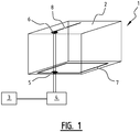
- Figure 1 shows a schematic perspective view of an electric supply network 1 arranged in a rectangular shaped chamber 2. Via a monitoring element 4 the network 1 is connected to a grid point 3 of a public electric power supply system. From the monitoring element 4, a mains line extends towards the chamber 2. The mains line includes distribution points 5, 6 branching off electric supply lines 7, 8 that are located near the floor and the ceiling respectively. Electric loads, such as domestic electrical appliances, can be connected to the electric supply lines 7, 8 in an inductive manner, as explained in more detail below.
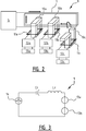
- FIG. 2 shows a schematic view of a part 9 of the electric supply network 1.
- a distribution point 5 is connected to an electric supply line 7 at the floor of the chamber 2.
- the distribution point 5 includes a capacitor that is arranged in series with the electric supply line 7.
- the electric supply line 7 is formed as an electrically conducting wire in a closed loop, so that the line 7 and the capacitor form a resonance circuit, also called LC-circuit or resonant tank.
- the distribution point 5 also includes a converter for converting electrical energy from the electrical source, e.g. a harmonic 50 Hz signal, into electrical energy having a central frequency at the resonance frequency of the resonant tank.
- the converter comprises an adaptive controller according to the invention for controlling energy supplied by an electrical source, viz. from the grid point 3, to the resonant tank connectable to an electric load.
- a magnetic ferrite kernel 10a-c can be shifted around a section of the electric supply line 7 that forms a primary coil.
- a secondary coil 11a-c extends so that a transformer element is formed.
- the secondary coil 11a-c is connected to an output converter 12a-c for converting the resonance signal to a harmonic signal that is suitable for powering the electrical load 13a-c, viz. a 230 V, 50 Hz signal. Since the electrical load 13a-c is inductively connected, there is no danger for an electrical short cut.
- FIG. 3 shows a simple electric scheme of the partial electric supply network 9.
- the resonant power converter including the controller for controlling electrical energy supplied to the resonant tank is represented by a controlled electrical source 14.
- the capacitor C r included in the grid point 5
- the inductor L r representing the coil 7.
- the resonant tank C r , L r is connected in series with electrical loads 13a-b.
- another number of electrical loads might be connected to the resonant tank, e.g. a single load or three loads.
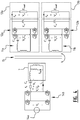
- Figure 4 shows a more detailed electric scheme of the partial electric supply network 9 and figure 5 exemplified a further simplified representation thereof.
- the inductance representing the electric supply line is replaced by a more complex inductor circuit 7 while the controlled electrical source 14 is separated in an electrical source 14a and a converter including a switching stage 14b and the controller for controlling the energy supplied to the resonant tank.
- the switching stage 14b is interconnected between terminals of the electrical source 14a and the resonant tank, respectively.
- the controller drives switching stage 14b switching elements, e.g. semiconductor switches, preferably high power MOSFET switches.
- the output converter 12a-b includes a switching stage that is controlled to generate a desired electrical signal from the resonance signal in the resonant tank.
- the secondary coil 11a is inductively connected to the primary coil via a magnetic coupling 15.
- Figure 6 shows an exemplary inductive connection of a load to the electric supply network 1.
- the coil of the electric supply line 7 has an elongated structure such that an offset between electrically conducting elements of the coil is small with respect to the length of said conducting elements, so that magnetic fields by the individual electrically conducting elements mutually substantially cancel.
- a first section 22 of the coil including conducting elements wherein, during use, electrical currents flow in a particular direction 20 surround a second section 23 of the coil including conducting elements wherein electrical currents flow in an opposite direction 21.
- the electric supply line 7 can be split, e.g. by using a clamp, at least locally, so that the inner section 21 of conducting elements or wires can be pulled locally out of the surrounding outer section 22 of elements.
- the magnetic ferrite kernel 10 can then be moved between the first and second section of the primary coil, so that the magnetic field can be coupled to the secondary coil 11.
- information of energy in the resonant tank is used as a basis for determining an energy amount to be supplied to the resonant tank.
- Figure 7 shows a number of energy plots associated with energy in the resonant tank (E Lr + E Cr ) as a function of time.
- the upper left plot shows the inductive energy E Lr as a function of time t.
- the upper right plot shows the capacitive energy E Cr as a function of time t.
- the lower left plot shows the total energy (inductive energy E Lr added to capacitive energy E Cr ) as a function of time.
- the total energy is mainly constant meeting an ideal situation wherein the amount of energy that is input to the resonant tank is equal to the energy that is output to the loads.
- the right lower graph of figure 7 exemplifies energy supplied by the source (E in ) and energy absorbed by the loads (E out ) changing in time. Due to a disturbance with respect to the ideal situation, a seemingly harmonic ripple is present in the total energy, as exemplified in the left lower graph of figure 7 .
- the lower right plot shows the energy E in (dashed line) that is input to the tank and the energy E out (solid line) that is output from the tank.
- the ripple in the total energy is associated with an instantaneous buffer component of the resonant tank energy.
- the instantaneous buffer component might be set strictly positive while the component is also minimized.
- the energy buffer component is used as a basis of information of energy in the resonant tank for the purpose of determining an energy amount to be supplied to the resonant tank.
- a filtered increase of resonant tank energy is integrated and subsequently controlled to a value depending on energy supplied to the resonant tank.
- said value might be related to the supplied energy in a linear or quadratic way.
- a proper relation of said value with the supplied energy can be established.
- the time scale of the filtering process is then different, preferably larger than the time scale of the integrating process, so that a filtered increase of the instantaneous energy buffer component is integrated and related to said value depending on energy supplied to the resonant tank.
- Resonant tank energy information can be determined by measuring at least one physical parameter associated with the resonant tank, e.g. an electrical current and/or an electrical voltage.
- a control objective such as relating a filtered increase of resonant tank energy to a value depending on energy supplied to the resonant tank, can be implemented in various ways, e.g. depending on the converter type and switch stage type.
- PWM pulse width modulation
- PSM phase-shift modulation
- FM frequency modulation
- QC quantum conversion
- control algorithms can be applied, both linear and non-linear.
- a controller based on sliding-mode control theory is explained in more detail below. In order to arrive at a specific controlling method, one or more control objects have to be rewritten as a valid sliding surface.
- Clamps 11a, 11b, 11c all in principle comprise the same configuration, for example in terms of the switch stage applied therein.
- the system as a whole, comprising cable 15, clamps 11, switching stages 12, 14, and other components, such as possibly externally arranged capacitors, may be referred to as an electronic power converter, connected to the resonant source.
- This disturbance of the ideal transfer is the buffer energy or surplus energy, which may be absorbed back by the source, referred to above in relation to figure 7 as a ripple due to a disturbance.
- buffer energy at any given time can be positive, defining a reserve or buffer, or negative, defining a shortage.
- it's possible to separate the buffer from the "perfect" DC-component where the idea is to ensure that the buffer component is always positive and thus that sufficient energy is present at all times for the load(s).
- the amount should be as low as possible and at the same time sufficient to avoid that the buffer component becomes negative, in which case control of the buffer component may be or become unstable.
- this representation is filtered, in which the differentiator t is referred to as being "slow".
- the filtered increase may be represented as an average or integrated value ⁇ E LC t ⁇ .
- control objective is to set the integrated filtered energy increase in the tank equal to a portion of the input energy.
- the resonant tank comprises all the necessary information to tune the source and load(s), without a need for communication across inductive couplings.
- the integrated change (differentiation) is used on different time scales, because a filter alters the time scale. Normally, integration of a differentiation should yield the original; mathematically not effective operation will have been performed, which is why the different time scales are of the essence.
- figure 4 In the configuration of figure 4 relates to a series-resonant converter, of which it is assumed that a single source is provided with a plurality of loads, but the representation of figure 5 allows for more complex configurations forming for example a parallel-resonant converter and/or comprising multiple sources and one or more than one load (see below in relation to figures 9 and higher).
- Pulse Width Modulation allows for "grasping" the input voltage using a fixed frequency, but for example at different times within one period of the frequency, such as at 30% of such a period from a a beginning thereof.
- Frequency modulation FM
- Combinations of the two modulations can be considered, as well.
- a disadvantage of PWM and of FM in current day resonant converters is the control range thereof in terms of power. For this reason an alternative modulation technique has been considered, which is Quantum Conversion (QC).
- QC Quantum Conversion
- Figure 9 exemplifies switch behavior in conjunction with modulation. Thick lines indicate current flowing and switches along a path of a thick line are conductive or open. All other switches are closed. This relates to the switching stages 12 at source 14a in figure 4 . In figure 9a energy is supplied to the circuit, and in figure 9b the source disconnected and output pins are short circuited.
- Figure 9c relates to energy flowing back into the source from the circuit.
- the modeled configuration of figure 4 is controlled by a power controller to implement the elementary switching modulation method of figure 9 , wherein the power controller sets each individual switch to be open or closed.
- SMCT sliding-Mode Control Theory
- SMCT is prima facie just one of many linear or non-linear algorithms, that may lead to a workable controller.
- SMCT is implemented, as it corresponds closely the type of control challenge underlying the present disclosure.
- SMCT is mainly based on defining a sliding surface to comply with three mathematical conditions, whereby control objectives of formula 2a or of formula 2b are transformed into a valid sliding surface.
- the input sliding surface is to relate to the input converter formed by switching stage 14b in figure 4 .
- the switching stages 12 in clamps 13 are also controlled on a basis of an output sliding surface.
- the DC input voltage is denoted V in and the control input is denoted by u p .
- the first right hand side term represents the buffer energy in the resonant tank when it is multiplied by the resonant current.
- the second term represents a fraction ⁇ of the supplied energy, when also multiplied by the resonant current. Note that both terms originally contained the same resonant current factor i r , which has been left out of the equation, but the energetic origin of the terms is still clear.
- Equation (13) contains the entire dynamics of the closed-loop system. Consulting linear system analysis, stability of the linear system is assured when ⁇ v i ⁇ r r ⁇ ⁇ 0 and 2 ⁇ c v i ⁇ ⁇ i 4 ⁇ c L r ⁇ > 0 .
- Condition (15) simply states that the input current must be larger than load current plus the current through the output filter capacitor.
- the input existence condition is the most interesting one.
- the conditions follow from the fact that the equivalent input control parameter must be between 0 and 1: 0 ⁇ u p,eq ⁇ 1. Setting the equivalent input larger than 0 leads to (16). r r > ⁇ 2 4 ⁇ c L r
- Equation (16) reflects the idea that the 'filtered' impedance of the averaged resonant tank must be smaller than the loss resistance in order to have enough real damping. In other words, the resonant tank must be able to release its energy fast enough.
- Expression (17) has the structure of an energy balance. On the right hand side, 'loss' terms are present. To be precise, from left to right: copper loss energy, virtual resonant tank energy, filter capacitor energy and load energy. The 'virtual' energy will be explained shortly. On the left hand side of (17) source terms are present. The left-most term is clearly the averaged input energy, while the right term represents the averaged stored resonant tank energy.
- the virtual energy term with ⁇ turns out to be a safety measure. It represents the dynamics of the resonant tank in essence.
- the momentary resonant tank energy can not be viewed as a term completely available (to compensate instantaneously) for the loss energies, because when the tank is empty it must be charged, before it can transfer energy again.
- the control parameter ⁇ is a function of i r (and vice versa) through the sliding surface and the state-space dynamics.
- i r is a function of its own derivative; see (13).
- the resulting first order differential equation is difficult to solve analytically, due to the nonhomogeneous sinusoidal output terms.
- Table 1 shows values for the parameters as introduced in Fig. 4 .
- Table I Parameter values for two-clamp cable prototype as referred to in Fig. 4 Symbol QUANTITY Value V i input DC voltage 600 [V] L r input side leakage inductance 40 [uH] r r Primary side winding resistance 2 [ ⁇ ] r o1 , r o2 output load resistances 240 [ ⁇ ] ⁇ c radial resonant frequency 100k [Hz] V o1 , V o2 required output voltages 240 [V] P o1 , P o2 required output powers 240 [W] n number of clamps 2
- the input sliding surface exists if (19) holds: 600 ⁇ ⁇ 2 4 2 ⁇ ⁇ 10 5 ⁇ 40 ⁇ 10 ⁇ 6 ⁇ ⁇ 480 ⁇ 600 ⁇ 2 ⁇ 1 2 > 2 ⁇ ⁇ 2 4 2 ⁇ ⁇ 10 5 ⁇ 40 ⁇ 10 ⁇ 6 480 ⁇ 600 ⁇ 2 ⁇ + 480 ⁇ 0.8 ⁇ ⁇ ⁇ 9.7
- ⁇ represents the fraction of the input energy that is used for the buffer energy in the tank
- the best (i.e., most energy efficient) solution for ⁇ is the minimum allowed value in (20).
- FIG. 8 shows a flow chart of an embodiment of the above described method.
- a controlling method is used for controlling energy supplied by an electrical source to a resonant tank connectable to an electric load.
- the method comprises the step 100 of determining an energy amount to be supplied based on information of energy in the resonant tank.
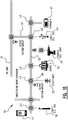
- Figure 10 exemplifies a more flexible network 30, enabling easy connection or disconnection of different types of loads, each having specific requirements in terms of connecting voltage or current, and sources, as well as storages.
- the system 30 can be connected to a DC grid 31 and a utility grid 35, from which the system can receive energy and to which energy can also be fed via respective connections 32, 36.
- the system has a back bone conductor 33, to which a source 34 and a buffer or storage 37 may be connected.
- loads may connected to the backbone conductor 33, such as a 12V (re)chargeable tooth brush 38, a 230V power tool 39, a 5V network apparatus 40, such as a 5V USB device, etc.
- a network controller 41 may be embodied in the form of an app on a mobile device.
- Each of these load apparatuses is connected to the backbone conductor 33, which could have a flexible or rigid form, via a coupler 42.
- couplers or nodes 42 are the same for source and loads.
- Nodes 42 are autonomous in the sense that no data transfer is required between nodes and / or between sources and nodes and/or between sources.
- the additional challenge of this more versatile configuration is how sources can determine autonomously (without data transfer) how much power they are to insert into the network over the backbone conductor 33, in a sufficient amount for all the loads to be able to function.
- WO-2011/031143 relating to a basic algorithm, system and method to determine a power need for all connected loads from a single source.
- the network in its entirety is configured to distribute power in accordance with a novel and inventive algorithm from one or more than one source to one or more than one load.
- the parameter ⁇ is constant and is determined beforehand, in advance of an actual use situation.
- the determination, beforehand, of the parameter ⁇ is based on expectations about maximum anticipated load power requirement (max ⁇ P 0 ⁇ ) in the network. Based on this assumption, control of the source in the network and the network itself will normally be robust and not lead to unstable operation. Determination beforehand of parameter ⁇ has a number of drawbacks.
- a fixed value of ⁇ can result in a limitation on the degree to which the full source power can be deployed, so that a maximum less than full source power is available to be released onto the network.
- the source cannot prevent that the assumed maximum load requirement max ⁇ P 0 ⁇ is exceeded, for example if more loads are connected to the backbone conductor 33.
- An optimal value of ⁇ is, at any given time, determined by an actual value of a sum of all loads ⁇ P 0 rather than any expectation about a maximum max ⁇ P 0 ⁇ thereof. This has for a consequence that for all situations, wherein ⁇ P 0 ⁇ max ⁇ P 0 ⁇ , efficiency is less than optimal for the network; more power is made available over the network than what is required to drive and supply power to the actually connected and combined loads.
- the graph in figure 11 provides relations between ⁇ and u p in accordance with equation (23), for three distinct load profiles ⁇ P 0 (1), ⁇ P 0 (2), and ⁇ P 0 (3). Also shown is max ⁇ P 0 , on which the prior art determination of a fixed ⁇ is based. It is evident, that in the prior art, ⁇ is determined at a level or value that is relatively high for all of the three distinct load profiles, indicating that energy supplied to the loads is too high for the actually connected loads according to each of the three load profiles ⁇ P 0 (1), ⁇ P 0 (2), and ⁇ P 0 (3). Thus efficiency is reduced.
- the source has no control over the amount or power requirement of connectable or even connected loads.
- the graph of figure 12 clearly exhibits that an unwanted unstable situation may occur unpredictably and undesirably in the prior art, if more loads are connected than anticipated or at least if the power requirement of the actually connected load(s) exceed(s) the anticipated max ⁇ P 0 ⁇ .
- WO-2011/031143 refers to adaptive control, but in fact, due to fixing ⁇ at a value determined a priori and then set, there's no temporal adaptation of ⁇ .
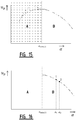
- the core issue underlying the present disclosure is how to enable determination of ⁇ min (t); how is it possible to determine between area's A (unstable) and B (stable) in figure 14 .
- the answer to this question is not in formula (22) above.
- This formula (22) only reveals a single point (at the questions mark "?" in Figure 14 ), while the rest of the shape and form of the graph associated with the determined point is unknown. In fact, the entire curve is unknown, which can also be the reason for the indication of a question mark in figure 14 .
- the bulge shape in dashed line is referred to above as an anomaly, this is not precisely correct as it is simply the curve in area A, having a higher MAX(u P ) than at the sought ⁇ min (t), thus rendering a strategy of maximizing u P to escape from area A unworkable.
- ⁇ P 0 does not vary faster than a rate of variation of ⁇ (t). This is considered to be a consequence of an actual difference in desired power delivery. This result in a further requirement: ⁇ ⁇ t ⁇ ⁇ ⁇ P o ⁇ t
- the adaptive controlling method for controlling energy supplied by an electrical source to a resonant tank connectable to an electric load can be performed using dedicated hardware structures, such as FPGA and/or ASIC components. Otherwise, the method can also at least partially be performed using a computer program product comprising instructions for causing a processor of the computer system to perform the above described one or more steps of the method according to the invention. All steps can in principle be performed on a single processor. However, it is noted that at least one step can be performed on a separate processor, e.g. the step of minimizing a buffer component of the resonant tank energy.
- a source can have a double role as energy can be supplied for example to a utility grid 35, then acting as a load, and at other times the utility grid 35 may supply energy.
- a battery that may charge or discharge to respectively act as a load and a source.
- the network primarily serves to transfer power from at least one source to a number of loads (including zero loads).
- the at least one source and the number of loads are connected inductively via nodes 42.
- Each node is autonomous, avoiding a need for any information exchange between nodes 42.
- WO-2011/031143 a basic approach is described to determine a required amount of power for all of the connected load nodes.
- a source node comprises a capacitor to define the resonant tank with the inductance of the network. In a case of a plurality of nodes, there's no singular source. Therefore the above sliding surface needs some adjustment, but still holds for a plurality of inductively coupled sources.
- An average current amplitude through the resonant tank inductance corresponds with the sum of the energy through the tank and energy stored in the tank.
- E source , j is the total input power.
- S j ⁇ j t ⁇ E source , j + ⁇ i # j E source , i ⁇ E network , stored the summation ⁇ i ⁇ j E source, i is not known for source j.
- Source node j has no direct knowledge about energy supplied by each of the other source nodes connected to the inductive network.
- This sliding surface is the definition of a relationship between power going through the tank, and power stored in the tank and elsewhere in storages or sources connected to the network.
- a node connecting a source to the network comprises a resonant capacitor to generate a resonant current.
- the reference to power going through the tank and stored in the tank is therefore to be interpreted as referring to the combined sources, inductively coupled to the network via the resonant capacitors in each of the source connecting nodes, and themselves therefore outside the network.
- ⁇ j (t) is not necessarily the same for each source node, and hence the subscript j, since for each source node the ratio ⁇ j (t) may converge to it's own optimum, as disclosed above.
- Figure 18 exhibits measured i r (or V cr ).
- Figure 19 exhibits the absolute values of the measured values.
- Energy stored in the tank per resonant half period can be determined based on peak-difference measurements. Energy passing through the tank per resonant half period can be characterized by the amplitude - peak difference measurements.
- V cr over the resonant capacities may be employed as an alternative for current through the network i r .
- a combination of both measurements may be employed.
- the amplitude measurements may follow the sequence from a to b to c to d.
- the peak difference measurement follow (a - ?) to (b - a) to (c - b) to (d - c).
- the peak difference measurements are based on i r or V Cr as these provide an indication of E network, stored , and the peak difference measurements reflect changes in the sliding surface equation. Successive values thereof change and the changes indicate changes in E network, stored and quantify the resulting changes ⁇ . By monitoring the peak differences, it's turned out to be possible to monitor ⁇ .
- the sources may be galvanic connected or inductively connected to the network via nodes, just like the loads, in contrast with the prior art according to WO-2011/031143 , where it was implicitly assumed that the source was connected directly and in series to the network itself.
- any defect of a source or source node would necessarily result in shut down, pending repairs.
- inductive coupling of the source(s) an adaptation of the remaining sources to supply a desired amount of energy to the network will be possible.
- Inductively connected source(s) (nodes) result in a consideration that the physical location of the source(s) (nodes) does not actually matter.
- a node may be equipped with a (resonant) capacitor, for example on the primary side of the source node. Equally, a resonant capacitor may be provided on the network side.
- the present disclosure also encompasses configurations having a plurality of sources physically connected to the network, and thus physically part of the network, rather than being inductively coupled thereto.
- One of the basic concepts of the present multi source approach of this disclosure is that one or more than one source will send a quasi-sinusoidal current through the network, potentially using one or more than one resonant capacitor.
- the sinusoidal shape of the network current an/or of the voltage over the (resonant) capacitor(s) reveals characteristics of the loads and other sources connected to the network, which can be used based on amplitude and peak-difference determination, because in a multi source configuration, the simplification of eq. 22 does not apply.
- the contribution of each source is not known at any of the other sources.
- the network current characteristics or those of the voltage V cr over the resonant capacities can yield the necessary information to allow each of the sources to optimise its corresponding contribution and maintain a sufficient supply over the network to each load.
- the invention is not restricted to the embodiments described herein. It will be understood that many variants are possible. For instance and without limitation: It is noted that the electric supply network according to the invention might in principle be arranged in building rooms having an arbitrary room geometry, such as in a house or in an office, or even outside where inductive coupling has specific benefits, such as less susceptibility to water, cold and the like.
- the resonant tank can be formed otherwise, e.g. as a capacitor arranged in parallel with the coil of the electric supply line. Further, the electrical loads might be arranged in parallel with the resonant tank.
- the resonant tank can not only be implemented as a first order LC-circuit but also as a higher order circuit including more than two reactive elements.
- one or more electrical loads might be connected to the resonant tank by using an electrically conducting connection without eliminating the operation of the adaptive controller according to the invention.
Landscapes
- Engineering & Computer Science (AREA)
- Computer Networks & Wireless Communication (AREA)
- Power Engineering (AREA)
- Supply And Distribution Of Alternating Current (AREA)
Description
- The present disclosure relates to a method, a controller and a network as set out in the appended claims.
- Prior art according to
WO-2011/031143 is acknowledged here. Therein, determination of a fixed relation between energy in a source and energy stored in a network is disclosed. The prior art is rigid and not sufficiently flexible to cope with loads and sources being added or removed. Moreover, by basing the approach of this prior art on a heaviest possible accumulated load (∑P0), efficiency could be improved on and losses reduced. - It is acknowledged here that
WO-2008/149275 discloses a prior art method and system. However, at least the features in the characterizing portion of the appended independent claim are novel over this prior art. - The present disclosure teaches adaptively balancing energy of the source (Esource) against energy in the network (Enetwork). According to the present disclosure, balancing is achieved by the steps in the characterizing portion of the appended independent method claim. Thereby, by willfully and continuously or iteratively, adapting a value of a balance factor α in α * Esource = Enetwork, the invention allows for ascertaining the effect in terms of approximation of a desired maximal minimum of α, and progressively adapting this α towards the desired maximal minimum value. A control input (up ) is varied, instead of directly the balance factor (a), under an assumption that

- A source could be considered required, but a load node may also verify, upon connection to a network, if any source or sufficient source capacity is available. Further, a number of loads can include no loads being connected to the network.
- Advantageous embodiments according to the invention are described in the appended dependent claims. More detailed information on the present disclosure is provided below.
- By way of example only, embodiments of the present invention will be described herein below, with reference to the accompanying figures in which
-
Fig. 1 shows a schematic perspective view of an electric supply network according to the invention; -
Fig. 2 shows a schematic view of a part of the electric supply network ofFig. 1 ; -
Fig. 3 shows a simple electric scheme of the partial electric supply network ofFig. 2 ; -
Fig. 4 shows a more detailed electric scheme of the partial electric supply network ofFig. 2 ; -
Fig. 5 a more schematic representation of the configuration according tofigure 4 ; -
Fig. 6 shows an inductive connection of a load to the electric supply network ofFig. 1 ; -
Fig. 7 shows a number of energy plots; -
Fig. 8 shows a flow chart of a prior method; -
Fig. 9 exemplifies switch behavior; -
Fig. 10 exhibits an exemplary flexible network with more freely connectable loads and at least one and possibly more than one source; - Fig.'s 11-17 exemplify graphs and curves for explaining considerations underlying the present disclosure;
- Fig.'s 18 and 19 exemplify characteristics of a network current or a voltage over a resonant capacitor.
- The figures are merely schematic views of preferred embodiments according to the present disclosure. In the figures, the same reference numbers may refer to the same and/or corresponding parts.
-
Figure 1 shows a schematic perspective view of anelectric supply network 1 arranged in a rectangularshaped chamber 2. Via amonitoring element 4 thenetwork 1 is connected to agrid point 3 of a public electric power supply system. From themonitoring element 4, a mains line extends towards thechamber 2. The mains line includesdistribution points electric supply lines electric supply lines -
Figure 2 shows a schematic view of a part 9 of theelectric supply network 1. Here, adistribution point 5 is connected to anelectric supply line 7 at the floor of thechamber 2. Thedistribution point 5 includes a capacitor that is arranged in series with theelectric supply line 7. Theelectric supply line 7 is formed as an electrically conducting wire in a closed loop, so that theline 7 and the capacitor form a resonance circuit, also called LC-circuit or resonant tank. Thedistribution point 5 also includes a converter for converting electrical energy from the electrical source, e.g. a harmonic 50 Hz signal, into electrical energy having a central frequency at the resonance frequency of the resonant tank. The converter comprises an adaptive controller according to the invention for controlling energy supplied by an electrical source, viz. from thegrid point 3, to the resonant tank connectable to an electric load. - In order to connect an electrical load to the
electric supply line 7, a magnetic ferrite kernel 10a-c can be shifted around a section of theelectric supply line 7 that forms a primary coil. Through the opening of the magnetic ferrite kernel 10a-c also asecondary coil 11a-c extends so that a transformer element is formed. Thesecondary coil 11a-c is connected to anoutput converter 12a-c for converting the resonance signal to a harmonic signal that is suitable for powering theelectrical load 13a-c, viz. a 230 V, 50 Hz signal. Since theelectrical load 13a-c is inductively connected, there is no danger for an electrical short cut. -
Figure 3 shows a simple electric scheme of the partial electric supply network 9. Here, the resonant power converter including the controller for controlling electrical energy supplied to the resonant tank is represented by a controlledelectrical source 14. Further, the capacitor Cr, included in thegrid point 5, is shown as well as the inductor Lr representing thecoil 7. The resonant tank Cr, Lr is connected in series withelectrical loads 13a-b. Obviously, also another number of electrical loads might be connected to the resonant tank, e.g. a single load or three loads. -
Figure 4 shows a more detailed electric scheme of the partial electric supply network 9 andfigure 5 exemplified a further simplified representation thereof. The inductance representing the electric supply line is replaced by a morecomplex inductor circuit 7 while the controlledelectrical source 14 is separated in anelectrical source 14a and a converter including aswitching stage 14b and the controller for controlling the energy supplied to the resonant tank. Theswitching stage 14b is interconnected between terminals of theelectrical source 14a and the resonant tank, respectively. The controller drives switchingstage 14b switching elements, e.g. semiconductor switches, preferably high power MOSFET switches. At the load side, theoutput converter 12a-b includes a switching stage that is controlled to generate a desired electrical signal from the resonance signal in the resonant tank. Thesecondary coil 11a is inductively connected to the primary coil via amagnetic coupling 15. -
Figure 6 shows an exemplary inductive connection of a load to theelectric supply network 1. Advantageously, the coil of theelectric supply line 7 has an elongated structure such that an offset between electrically conducting elements of the coil is small with respect to the length of said conducting elements, so that magnetic fields by the individual electrically conducting elements mutually substantially cancel. In the shown embodiment inFig. 5 , afirst section 22 of the coil including conducting elements wherein, during use, electrical currents flow in aparticular direction 20, surround asecond section 23 of the coil including conducting elements wherein electrical currents flow in anopposite direction 21. By arranging the coil in such a way, afirst section 22 of conducting elements or wires surround asecond section 21 of conducting elements or wires, and a net magnetic field outside theelectric supply line 7 substantially vanish. Further, theelectric supply line 7 can be split, e.g. by using a clamp, at least locally, so that theinner section 21 of conducting elements or wires can be pulled locally out of the surroundingouter section 22 of elements. Themagnetic ferrite kernel 10 can then be moved between the first and second section of the primary coil, so that the magnetic field can be coupled to the secondary coil 11. - During operation of the adaptive controller according to the invention, information of energy in the resonant tank is used as a basis for determining an energy amount to be supplied to the resonant tank.
-
Figure 7 shows a number of energy plots associated with energy in the resonant tank (ELr + ECr) as a function of time. The upper left plot shows the inductive energy ELr as a function of time t. Similarly, the upper right plot shows the capacitive energy ECr as a function of time t. The lower left plot shows the total energy (inductive energy ELr added to capacitive energy ECr) as a function of time. As expected, the total energy is mainly constant meeting an ideal situation wherein the amount of energy that is input to the resonant tank is equal to the energy that is output to the loads. The right lower graph offigure 7 exemplifies energy supplied by the source (Ein) and energy absorbed by the loads (Eout) changing in time. Due to a disturbance with respect to the ideal situation, a seemingly harmonic ripple is present in the total energy, as exemplified in the left lower graph offigure 7 . The lower right plot shows the energy Ein (dashed line) that is input to the tank and the energy Eout (solid line) that is output from the tank. - It is noted that the ripple in the total energy is associated with an instantaneous buffer component of the resonant tank energy. In the process of controlling an amount of energy to be supplied to the tank, the instantaneous buffer component might be set strictly positive while the component is also minimized. Thus, the energy buffer component is used as a basis of information of energy in the resonant tank for the purpose of determining an energy amount to be supplied to the resonant tank. Advantageously, a filtered increase of resonant tank energy is integrated and subsequently controlled to a value depending on energy supplied to the resonant tank. As an example, said value might be related to the supplied energy in a linear or quadratic way. Depending on a particular application, a proper relation of said value with the supplied energy can be established. Further, the time scale of the filtering process is then different, preferably larger than the time scale of the integrating process, so that a filtered increase of the instantaneous energy buffer component is integrated and related to said value depending on energy supplied to the resonant tank.
- Resonant tank energy information can be determined by measuring at least one physical parameter associated with the resonant tank, e.g. an electrical current and/or an electrical voltage.
- A control objective, such as relating a filtered increase of resonant tank energy to a value depending on energy supplied to the resonant tank, can be implemented in various ways, e.g. depending on the converter type and switch stage type. As an example, pulse width modulation (PWM), phase-shift modulation (PSM) or frequency modulation (FM) can be employed. Also a combination is possible. As a further example, a quantum conversion (QC) modulation method can be used wherein the modulation is controlled synchronous with the resonance frequency of the resonant tank.
- Further, different control algorithms can be applied, both linear and non-linear. As an example, a controller based on sliding-mode control theory is explained in more detail below. In order to arrive at a specific controlling method, one or more control objects have to be rewritten as a valid sliding surface.
- In a state-space annotation, the configuration of
figures 4 and5 may be expressed as follows:

- It is intended to transport energy from the
source 14a, Vi infigures 4 and5 to the load(s) as efficiently as possible. Power control may be achieved by appropriate driving of switchingstage 14b.Clamps cable 15, clamps 11, switchingstages 12, 14, and other components, such as possibly externally arranged capacitors, may be referred to as an electronic power converter, connected to the resonant source. - By modeling
figure 4 into the simplified representation offigure 5 , it becomes apparent that monitoring the tank's behavior may result in appropriate control of the tank's output. The resonant tank, modeled by the dashed lines box infigure 5 , has relevant information and in any case all information necessary, for tuning input energy Ein and the total output energy ∑Eout (=E clamp 1 + E clamp.... . + Eclamp n). Power supplied by the resonant tank and energy stored therein may then be expressed as follows:

- The amount of energy ELC in the resonant tank at any given time consists essentially of two components, of which one represents ideal energy transfer at Ein = ∑Eout, where the other component is a disturbance of the ideal energy transfer. This disturbance of the ideal transfer is the buffer energy or surplus energy, which may be absorbed back by the source, referred to above in relation to
figure 7 as a ripple due to a disturbance. - In principle, buffer energy at any given time can be positive, defining a reserve or buffer, or negative, defining a shortage. However, it's possible to separate the buffer from the "perfect" DC-component, where the idea is to ensure that the buffer component is always positive and thus that sufficient energy is present at all times for the load(s). To avoid this leading to waste of energy, the amount should be as low as possible and at the same time sufficient to avoid that the buffer component becomes negative, in which case control of the buffer component may be or become unstable.
- The buffer component represents an increase of energy in the tank, being

- However, this representation is filtered, in which the differentiator t is referred to as being "slow". The filtered increase may be represented as an average or integrated value

- By equating an integral of the filtered energy increase and a positive constant will ensure that the energy component of the buffer remains constant, in which case there will be at all times a surplus of energy for the loads. However, at the same time it is desirable to reduce this surplus to as low a constant value as possible. It has been found that an amplitude of the ripple, referred to above in relation to
figure 7 , in relation to the constant energy component of the buffer is responsible for how low the constant of the buffer component can be set. The magnitude of the4 ripple superimposed on the average buffer component is then dependent on absolute or total input power. For this reason the buffer component is not just set to just any constant, but to have a relation with the input energy: constant ' Ein. In summary, the control objective is to set the integrated filtered energy increase in the tank equal to a portion of the input energy. This can be expressed in one of several formulae, such as:

- In any case, to arrive at this control objective, it was necessary to understand and utilize, that the resonant tank comprises all the necessary information to tune the source and load(s), without a need for communication across inductive couplings. To this end the integrated change (differentiation) is used on different time scales, because a filter alters the time scale. Normally, integration of a differentiation should yield the original; mathematically not effective operation will have been performed, which is why the different time scales are of the essence.
- In the configuration of
figure 4 relates to a series-resonant converter, of which it is assumed that a single source is provided with a plurality of loads, but the representation offigure 5 allows for more complex configurations forming for example a parallel-resonant converter and/or comprising multiple sources and one or more than one load (see below in relation tofigures 9 and higher). - Even implementation of a transformer is not a necessary precondition for implementing the invention according to the present application.
- For the switching stages 12, 14, a number of modulation methods are available. Pulse Width Modulation (PWM) allows for "grasping" the input voltage using a fixed frequency, but for example at different times within one period of the frequency, such as at 30% of such a period from a a beginning thereof. Frequency modulation (FM) can "grasp" the input voltage using a variable frequency. Combinations of the two modulations can be considered, as well. A disadvantage of PWM and of FM in current day resonant converters is the control range thereof in terms of power. For this reason an alternative modulation technique has been considered, which is Quantum Conversion (QC). When implementing Quantum Conversion, switching is performed precisely in synch with the resonant frequency of the tank. In theory, the control range is infinite, when implementing Quantum Conversion.
-
Figure 9 exemplifies switch behavior in conjunction with modulation. Thick lines indicate current flowing and switches along a path of a thick line are conductive or open. All other switches are closed. This relates to the switching stages 12 atsource 14a infigure 4 . Infigure 9a energy is supplied to the circuit, and infigure 9b the source disconnected and output pins are short circuited. -
Figure 9c relates to energy flowing back into the source from the circuit. - The modeled configuration of
figure 4 is controlled by a power controller to implement the elementary switching modulation method offigure 9 , wherein the power controller sets each individual switch to be open or closed. - Several distinct elementary control methods are available, which allow division into several groups, such as linear and non-linear algorithms. An example of a non-linear method is based on so-called "Sliding-Mode Control Theory" (SMCT). Although SMCT is prima facie just one of many linear or non-linear algorithms, that may lead to a workable controller. In the present instance, SMCT is implemented, as it corresponds closely the type of control challenge underlying the present disclosure. SMCT is mainly based on defining a sliding surface to comply with three mathematical conditions, whereby control objectives of formula 2a or of formula 2b are transformed into a valid sliding surface.
- The input sliding surface is to relate to the input converter formed by switching
stage 14b infigure 4 . The switching stages 12 in clamps 13 are also controlled on a basis of an output sliding surface. - Herein below, first a candidate input sliding surface is determined. Then it will be proven when (for which α) the candidate sliding surface complies with conditions under the implemented theory. Finally, an exemplary configuration is proposed, and the minimal and therefore optimal α is determined.
- A key observation is that the tank transfers energy from one quantum period to the next, although each of the tank components discharges completely during a (quantum) period. Next important observation is the fact that the resonant inductor Lr can not transfer energy between periods, because by definition a consecutive period starts with zero current, and therefore with an energetic empty resonant inductor. The buffer energy of formula 2a above is developed into:

- As schematically indicated at the formula (3) above, the contribution of ir · L (dir/dt) is negligible and can be approximated as 0 (zero). The right-hand side of (2a) is provided in (4).

- The input sliding surface - related to the input converter - then follows in (5) as the difference of equations (3) and (4) .

- The purpose of (5) is to become zero, which implies that (5) can be divided by the average of ir .

- While surface (6) is the basic sliding surface, a rewritten form is better suited for mathematical analysis. First step is to rewrite the second right hand term in (6) into (7).

- In (7), the DC input voltage is denoted Vin and the control input is denoted by up . The left term is rewritten by noting that


- The motivation behind the (close) approximation (8) is that applying the low-pass filter on νr sgn(ir ) is equivalent to the average of ir (up to the constant C), when accepting the loss of phase information between voltage and current. Though, one of the strengths of quantum conversion is that phase information is not used at all, because switching occurs only at zero resonant current. If for example the control method would be applied to a different conversion method than quantum conversion (e.g., PWM or FM, see previous paragraph), (8) would not be true.
- Substitution of (7) and (8) in sliding surface (6) leads to the rewritten sliding surface (9). Note that phase information is also discarded from the second right hand term by only using the magnitude of the filter.

- Interpreting (9), the first right hand side term represents the buffer energy in the resonant tank when it is multiplied by the resonant current. The second term represents a fraction α of the supplied energy, when also multiplied by the resonant current. Note that both terms originally contained the same resonant current factor ir, which has been left out of the equation, but the energetic origin of the terms is still clear.
- The intuitive reason that (9) 'works' is that the supplied energy reacts little more slowly than the buffer tank energy. For example, adopting the common control law (10), it is clear that the buffer will grow faster than the average supplied energy when Sp >0 and as a result Sp becomes <0, and vice versa.

- In the following a formal proof of the validness of (candidate) sliding surface (9) is provided. In sliding-mode control theory the following 3 conditions must be formally met to guarantee stable closed-loop operation: Reaching condition, Existence condition and Stability condition. Reaching considers the fact that the control law must assure to reach the sliding surface (in finite time) starting from all possible initial states. Existence means that the system dynamics must be able to stay at the sliding surface once it is reached. The stability condition considers internal stability of the closed-loop system. Sliding mode control design effectively linearizes the non-linear plant system, but those invisible reminiscent terms must be checked on stability also.
- We start with forming the closed-loop system dynamics with the help of the sliding surfaces. First step is to put Sp equal to zero. Rewriting (9) with Sp=0 results in (11).

- Substituting for


- Substituting (12) in (0a) leads to a linear first-order -2 differential expression in


- Equation (13) contains the entire dynamics of the closed-loop system. Consulting linear system analysis, stability of the linear system is assured when

- Rewriting the latter equations leads to the stability condition for α in (14).

- This shows the upper bound of α for which the system is stable. Result of choosing α larger than the bound in (14) is an unlimited increase of stored energy in the primary circuit. There is no lower bound from a stability point of view, because we look from the primary side (assuming the secondary side dynamics being situated at the sliding surface) and the system will converge to zero-power throughput in the worst case. See Fig. x2 for an illustration.
- The existence conditions will put a lower bound for α, in order to assure stable regime; enough input power to supply the secondary sides. For the outputs the existence conditions are straightforward:

- Condition (15) simply states that the input current must be larger than load current plus the current through the output filter capacitor.
- The input existence condition is the most interesting one. The conditions follow from the fact that the equivalent input control parameter must be between 0 and 1: 0< up,eq <1. Setting the equivalent input larger than 0 leads to (16).

- Note that in (16) the radial frequency is the cut-off frequency of the low-pass filter and not the resonant frequency. Equation (16) reflects the idea that the 'filtered' impedance of the averaged resonant tank must be smaller than the loss resistance in order to have enough real damping. In other words, the resonant tank must be able to release its energy fast enough.
- The remaining condition, up,eq <1, reveals when the buffer-energy percentage in the resonant tank is enough to assure local stability. Substituting for up,eq the expression in (12) and rewriting, the final condition follows in (17).

- Expression (17) has the structure of an energy balance. On the right hand side, 'loss' terms are present. To be precise, from left to right: copper loss energy, virtual resonant tank energy, filter capacitor energy and load energy. The 'virtual' energy will be explained shortly. On the left hand side of (17) source terms are present. The left-most term is clearly the averaged input energy, while the right term represents the averaged stored resonant tank energy.
- The virtual energy term with α turns out to be a safety measure. It represents the dynamics of the resonant tank in essence. The momentary resonant tank energy can not be viewed as a term completely available (to compensate instantaneously) for the loss energies, because when the tank is empty it must be charged, before it can transfer energy again.
- The control parameter α is a function of
i r (and vice versa) through the sliding surface and the state-space dynamics. The only problem to advance further into an explicit condition for α is thati r is a function of its own derivative; see (13). The resulting first order differential equation is difficult to solve analytically, due to the nonhomogeneous sinusoidal output terms. - The following simplification is justified by the fact that interest is in a (rough) design guidance value for α ; in practice the value for α will be tuned by observation. Returning to expression (13), the simplification consists of assuming zero ripple in ir(t), which makes the left hand side of (13) equal to 0. Rewriting (13) results in an approximate expression for
i r as a function of α:
- In (18), Poj replaces


- In the following the previous design conditions are applied to a design
example. Table 1 shows values for the parameters as introduced inFig. 4 .Table I Parameter values for two-clamp cable prototype as referred to in Fig. 4 Symbol QUANTITY Value Vi input DC voltage 600 [V] Lr input side leakage inductance 40 [uH] rr Primary side winding resistance 2 [Ω] ro1, ro2 output load resistances 240 [Ω] ω c radial resonant frequency 100k [Hz] Vo1, Vo2 required output voltages 240 [V] Po1, Po2 required output powers 240 [W] n number of clamps 2 - Stability is assured when (14) applies:

- The sliding surface for the output exists if (15) holds, where expression (18) is substituted for
ir :
- The input sliding surface exists if (19) holds:

- Combining the previous conditions, the design solution gives:

- Whereas α represents the fraction of the input energy that is used for the buffer energy in the tank, the best (i.e., most energy efficient) solution for α is the minimum allowed value in (20).
-
Figure 8 shows a flow chart of an embodiment of the above described method. A controlling method is used for controlling energy supplied by an electrical source to a resonant tank connectable to an electric load. The method comprises thestep 100 of determining an energy amount to be supplied based on information of energy in the resonant tank. - Up to here the description relates to setting an α to be robust and essentially fixed, at a level for safe operation, basically based on a galvanic connection of a source to the network.
- Building on the above theoretical basis, it was already indicated at a reference to
figure 5 that the principles underlying the determination of a minimal and thus optimal α could additionally apply to a configuration with more than one source and one or more than one load. Additionally, a fixed α results in potentially rigid configurations, whilst it would be desirable to be able to use the system and method of the present disclosure also under varying circumstances, such as adding or removing loads and / or sources, with the same efficiency and keeping to the desires and objectives as set out above, of minimizing α, while at the same time preventing instability of the control and ensuring that the buffer component doesn't become negative.Figure 10 exemplifies a moreflexible network 30, enabling easy connection or disconnection of different types of loads, each having specific requirements in terms of connecting voltage or current, and sources, as well as storages. Thesystem 30 can be connected to aDC grid 31 and autility grid 35, from which the system can receive energy and to which energy can also be fed viarespective connections back bone conductor 33, to which asource 34 and a buffer orstorage 37 may be connected. Several types of loads may connected to thebackbone conductor 33, such as a 12V (re)chargeable tooth brush 38, a230V power tool 39, a5V network apparatus 40, such as a 5V USB device, etc. Anetwork controller 41 may be embodied in the form of an app on a mobile device. Each of these load apparatuses is connected to thebackbone conductor 33, which could have a flexible or rigid form, via acoupler 42. In principle couplers ornodes 42 are the same for source and loads.Nodes 42 are autonomous in the sense that no data transfer is required between nodes and / or between sources and nodes and/or between sources. As a consequence the additional challenge of this more versatile configuration is how sources can determine autonomously (without data transfer) how much power they are to insert into the network over thebackbone conductor 33, in a sufficient amount for all the loads to be able to function. Herein above prior art is described, which originates from the inventor's own previous publicationWO-2011/031143 , relating to a basic algorithm, system and method to determine a power need for all connected loads from a single source. - In order to allow for a desired degree of versatility, further developments have been contemplated. Therein, the network in its entirety is configured to distribute power in accordance with a novel and inventive algorithm from one or more than one source to one or more than one load.
- Again it is assumed that a power requirement of all loads ∑P0 together is available or can at least be deduced from the energy in the source, which may be a resonant tank or an arbitrary energy buffer of the network. Temporary energy storage or buffering appears to be very important though possibly not essential to the invention. This may point to an inductive network or as an alternative, potentially an adequate buffer connected to the
backbone conductor 33 may suffice. In any case, where in the following description reference is made to a resonant tank in an inductive network, these exemplary features are not to be taken as limitations on the scope of protection. - A sliding surface equation for a source may be expressed, in line with the principles underlying the prior art discussed above, see formula (4) above. However, this is where all comparison ends:

- Namely, in the prior art technology described above, the parameter α is constant and is determined beforehand, in advance of an actual use situation. The determination, beforehand, of the parameter α is based on expectations about maximum anticipated load power requirement (max{∑P0}) in the network. Based on this assumption, control of the source in the network and the network itself will normally be robust and not lead to unstable operation. Determination beforehand of parameter α has a number of drawbacks.
- A fixed value of α can result in a limitation on the degree to which the full source power can be deployed, so that a maximum less than full source power is available to be released onto the network.
- The source cannot prevent that the assumed maximum load requirement max{∑P0} is exceeded, for example if more loads are connected to the
backbone conductor 33. - An optimal value of α is, at any given time, determined by an actual value of a sum of all loads ∑P0 rather than any expectation about a maximum max{∑P0} thereof. This has for a consequence that for all situations, wherein ∑P0 < max{∑P0}, efficiency is less than optimal for the network; more power is made available over the network than what is required to drive and supply power to the actually connected and combined loads.
- Formula (21) does not suffice to tune α in operation and continuously to an instantaneous optimum thereof, taking the actually connected combined loads into account. Surprisingly, as it turns out, the information missing to be able to achieve instantaneous adaptation of α has been found to reside in formula 18 above, which is reproduced here for completeness, brevity and clarity:

- By further developing formula (21) above, it is obtained that:


- The graph in
figure 11 provides relations between α and up in accordance with equation (23), for three distinct load profiles ∑P0(1), ∑P0(2), and ∑P0(3). Also shown is max∑P0, on which the prior art determination of a fixed α is based. It is evident, that in the prior art, α is determined at a level or value that is relatively high for all of the three distinct load profiles, indicating that energy supplied to the loads is too high for the actually connected loads according to each of the three load profiles ∑P0(1), ∑P0(2), and ∑P0(3). Thus efficiency is reduced. - In relation to each profile ∑P0(1), ∑P0(2), and ∑P0(3), there's a minimal α (α min, x), at which there's certainty that the source and the controller thereof insert precisely enough power into the network for all actually connected loads in combination, and as little more as is needed to prevent with certainty that the unstable state, referred to above, occurs.
- On the other hand, to be able to set a beforehand determined value of α as a fixed parameter, this value needs to be set higher than a maximum value of α at any load situation, which could be referred to as max(α min, x). Such a "maximal minimum" would therefore correspond with a maximum load max∑P0. At such a value of α, network efficiency would be less than optimal for all of the potentially realistic power profiles. However, this issue can be addressed using an adaptive approach to α. In
figure 11 , the precise load profile is not known beforehand. However, it is known in advance of any load profile potentially occurring, that the following functioning occurs:α = αmin,x ↔ stabiel & η max stability and high efficiency α > αmin,x ↔ stabiel & η↓ Stability, but reduced η α < αmin,x ↔ instabiel Unstable, or even instable - The source has no control over the amount or power requirement of connectable or even connected loads. As a consequence, stabile and highly efficient, inefficient but stable and unstable behavior may occur, in particular respectively when:


- However, it is uncertain in which area or zone operation of the system is, when it isn't known how many loads are actually connected and what the respective power requirement(s) thereof is/are, as there is no communication about such aspects over the
backbone conductor 33. - The graph of
figure 12 clearly exhibits that an unwanted unstable situation may occur unpredictably and undesirably in the prior art, if more loads are connected than anticipated or at least if the power requirement of the actually connected load(s) exceed(s) the anticipated max{∑P0}. - One further result of the prior art worst case approach, according to which the predetermined fixed α, which is calculated and then fixed a priori, may be much higher than required for an actually connected (amount of) load at any given time (αa priori >> αmin(t)), as shown in
figure 13 , is considerable efficiency loss and costs, although the system remains to be stable. - The above described basic disclosure of
WO-2011/031143 refers to adaptive control, but in fact, due to fixing α at a value determined a priori and then set, there's no temporal adaptation of α. - Therefore, the core issue underlying the present disclosure is how to enable determination of αmin(t); how is it possible to determine between area's A (unstable) and B (stable) in
figure 14 . The answer to this question is not in formula (22) above. This formula (22) only reveals a single point (at the questions mark "?" inFigure 14 ), while the rest of the shape and form of the graph associated with the determined point is unknown. In fact, the entire curve is unknown, which can also be the reason for the indication of a question mark infigure 14 . - The solution to this challenge turned out to reside in formula (18) above, as already indicated. This will be explained herein below.
- In area B of
figure 14 , the total load power may be assumed constant, based for area B on:
- This formula (24) results, based on formula (23) above, in

- This formula (25) only holds in area B of
figures 14 - 16 . By continuously varying α, which can be achieved by varying up, the following algorithm in formula (26) provides a proper indication of the direction (decrease /increase) in which α needs to be varied further to most closely approximate the most optimal and stable value:
- As long as the criterion of formula (25) is complied with, it may be established that:

- This is precisely what was sought. However, from the bulge shaped anomaly in the left hand side of
figure 15 , indicated by the dashed line therein, it will be evident to the skilled person that the criterion of formulae 25 may be complied with, and that it could be then erroneously be assumed that formula (27) also holds. However, based on the notion that formula (25) only holds in area B offigures 14 - 16 , the error can be prevented. Apparently, it does not suffice to determine αmin(t) by maximizing up. After all, in area A infigures 14 and15 , the shape of the graph is not fixed and may vary, which is why the bulge shaped anomaly is represented in the dashed line graph shape infigure 15 . The reason for this is that in area A the load power has become a function of α and consequently of the power in time, depending on α: ∑P0(α, t). In other words, the maximum of up could be in area A, as shown at the bulge shaped, dash lined anomaly in the graph offigure 15 , as indicated in the dashed line, even though the conditions of formulae (25) and (26) are met. - Although the bulge shape in dashed line is referred to above as an anomaly, this is not precisely correct as it is simply the curve in area A, having a higher MAX(uP) than at the sought αmin(t), thus rendering a strategy of maximizing uP to escape from area A unworkable.
- The shape of the curve [α, uP] in area B of
figures 14 and15 is to a considerable degree fixed, and is defined inequation 23 above. However, as an absolute value of ∑P0 is unknown, the controller is unable to determine a current position on the curve in area B, as shown infigure 16 . On the other hand, surprisingly, this position does not necessarily have to be determined precisely in order to arrive at a determination of αmin(t). To determine an αmin(t) it suffices - again surprisingly - to have the shape of the curve infigure 16 . By slightly varying α, from α1 to α2 infigure 16 or vice versa, the effect on uP becomes apparent, as it changes frompoint 1 on the curve to point 2 (or vice versa). Thus, by varying α, the shape of the curve becomes apparent, at least in and for area B, and then α can be adapted further to approximate αmin(t) better, by hollowing the shape of the curve in the predicted direction, which is to the left infigure 16 , by decreasing the value of α. In fact this finding is the algorithm of formula (26) above. - In contrast, and as shown in
figure 17 , the shape of the curve in area A to the left of the unknown αmin(t) is unknown.Figure 17 exemplifies some of the erratic shapes that the curve can have in area A. This is understandable from the fact that the slidingsurface equation 22 above does not hold in area A. Most often, the behavior may followcurve 2 infigure 17 . However, the occurrence ofcurve 1 cannot be excluded. - As a first strategy to try to resolve this matter, the skilled person may decide to maximize uP, which could resolve for
curves figure 17 , but not forcurve 1. Although this obvious strategy may succeed in some situations, it would not be robust for all situations, such as forcurve 1 infigure 17 . - To resolve this issue, surprisingly the solution is provided on the basis of the fact that in area A, behavior does not follow the sliding
surface equation 22 above, and behavior does not follow formula (25). In other words, in area A the curve is not the one of area B, and/or formula (25) does not hold in area A, because ∑P0 varies in area A. A reason why the curve can exhibit erratic shapes in area A is because instantaneous power input intoconductor 33 at any given time is Pi = uP * Vi * ir. In the slidingsurface equation 22 above, resonant current is shared by all sources and loads. All of the deductions fromequation 22 rely on the assumption of a small ripple on the amplitude of the resonant current ir, whereas this holds true to a larger or lesser extent, depending on the low-level switch-modulation method. - In short, and in simplified representation, when a series uP = [1, 0, 1] (on average 2/3) occurs with averaged ir = [1, 3, 1], this yields less input power Pi = 2 than in a situation wherein up = [0, 1, 0] (on average 1/3) and averaged ir = [1, 3, 1], yielding Pi = 3. As a consequence, it is possible to provide relatively less energy at a relatively high average of uP.
- Further, it is assumed that ∑P0 does not vary faster than a rate of variation of α(t). This is considered to be a consequence of an actual difference in desired power delivery. This result in a further requirement:

- Yet, α(t) should not vary too quickly, as formula (22) must have time to stabilize to zero, which involves reaching phase in sliding mode control:

- In summary: for a predetermined α, this will be robust only if ∑P0(∞) < max∑P0, but involves a loss of efficiency η if at any given time ∑P0(t) < max∑P0. The minimum of α at any given time can always be robust and at all times secure optimal network efficiency. In order to determine, it is proposed to vary α, or varying any of
- In case that α is in the undesired area A, the algorithm of

- The adaptive controlling method for controlling energy supplied by an electrical source to a resonant tank connectable to an electric load can be performed using dedicated hardware structures, such as FPGA and/or ASIC components. Otherwise, the method can also at least partially be performed using a computer program product comprising instructions for causing a processor of the computer system to perform the above described one or more steps of the method according to the invention. All steps can in principle be performed on a single processor. However, it is noted that at least one step can be performed on a separate processor, e.g. the step of minimizing a buffer component of the resonant tank energy.
- Reverting to the configuration of
figure 10 , multiple sources are connected, such asDC grid 31,source X 34,utility grid 35 andstorage X 37. A source can have a double role as energy can be supplied for example to autility grid 35, then acting as a load, and at other times theutility grid 35 may supply energy. The same holds for a battery that may charge or discharge to respectively act as a load and a source. - The network primarily serves to transfer power from at least one source to a number of loads (including zero loads). The at least one source and the number of loads are connected inductively via
nodes 42. Each node is autonomous, avoiding a need for any information exchange betweennodes 42. In the inventor's own previous prior art disclosureWO-2011/031143 a basic approach is described to determine a required amount of power for all of the connected load nodes. - However, in
WO-2011/031143 , the source was coupled to the network via a galvanic connection. Referring back to formulae (1c) and (1d) above, P designated power transferred through the tank and E designated energy stored on the tank. Through deductions a sliding surface was determined that
- As mentioned above, the starting point of the disclosure of
WO-2011/031143 is a galvanic connection of the source to the network. Below, this starting point does not apply and the source or sources will be connected through a galvanic connection or inductively to the network. For the below discussion, an inductive connection is assumed, though the disclosure is not limited thereto. To this end a source node comprises a capacitor to define the resonant tank with the inductance of the network. In a case of a plurality of nodes, there's no singular source. Therefore the above sliding surface needs some adjustment, but still holds for a plurality of inductively coupled sources.
- A preceding implementation of the sliding
surface equation 21 above is provided informula 22, based on a simplification:
- However, here (with more than one source):


- An average current amplitude through the resonant tank inductance corresponds with the sum of the energy through the tank and energy stored in the tank. A more formal definition of eq. 34 is therefore:

- Rewriting eq. 35 to the format of eq. 21 results in:


- In an inductively coupled multi-source configuration, for a single source node j, the sliding surface can be expressed as:

- Therein, Esource, j is the total input power. In a configuration of a plurality of sources:

- The challenge in this approach resides in the fact that in the sliding surface j for multiple sources:

- As a solution to this challenge, the summation ∑i≠j E source,i is determined indirectly. By reverting to sliding surface equation (21):

- The basic idea of this sliding surface is the definition of a relationship between power going through the tank, and power stored in the tank and elsewhere in storages or sources connected to the network.
- It should be noted that in case of multiple sources, these may be approximated as a single distributed source. Thus reference here to the tank implies the combined sources connected to the network, but not forming part of the network. The distributed sources are each connected inductively to the network in order to avoid - in the case of direct connection of the multiple sources - that the entire network needs to be shut down when one source fails. As a consequence, a node connecting a source to the network comprises a resonant capacitor to generate a resonant current. Further, the reference to power going through the tank and stored in the tank is therefore to be interpreted as referring to the combined sources, inductively coupled to the network via the resonant capacitors in each of the source connecting nodes, and themselves therefore outside the network.
- The ratio between these powers through and stored in the "tank" defines as, assuming S = 0 for the most efficient result:

- Again reverting to eq. 21, yields:

- Since it is of no importance which source (node) delivers the required amount of energy. As a consequence each individual source node can rely on the same surface form:

- Therein, αj(t) is not necessarily the same for each source node, and hence the subscript j, since for each source node the ratio αj(t) may converge to it's own optimum, as disclosed above.
- Again assuming S=0, based on

- In order to be able to determine Enetwork, throughput this term must be separated from Enetwork, stored, again using eq. 22:

- At the stage of developments of obtaining eq. 22, the aforementioned separation was not yet necessary, since for a single source the value of Enetwork, throughput is known. For a plurality of sources (source nodes) it will therefore be necessary to determine (by measurement) peak-difference values, in addition to amplitude measurement of ir. These measurements together characterize the behaviour of the combined total tank or combination of source nodes.
-
Figure 18 exhibits measured ir (or Vcr).Figure 19 exhibits the absolute values of the measured values. - Energy stored in the tank per resonant half period can be determined based on peak-difference measurements. Energy passing through the tank per resonant half period can be characterized by the amplitude - peak difference measurements.
- For these measurements, as an alternative for ir, voltage Vcr over the resonant capacities may be employed as an alternative for current through the network ir. To enhance robustness and accuracy, a combination of both measurements may be employed.
- In
figure 19 , the amplitude measurements may follow the sequence from a to b to c to d. The peak difference measurement follow (a - ?) to (b - a) to (c - b) to (d - c). The peak difference measurements are based on ir or VCr as these provide an indication of Enetwork, stored, and the peak difference measurements reflect changes in the sliding surface equation. Successive values thereof change and the changes indicate changes in Enetwork, stored and quantify the resulting changes α. By monitoring the peak differences, it's turned out to be possible to monitor α. - In relation to the multi source approach, it is noted that the sources may be galvanic connected or inductively connected to the network via nodes, just like the loads, in contrast with the prior art according to
WO-2011/031143 , where it was implicitly assumed that the source was connected directly and in series to the network itself. In a multi-source approach, any defect of a source or source node would necessarily result in shut down, pending repairs. By inductive coupling of the source(s), an adaptation of the remaining sources to supply a desired amount of energy to the network will be possible. - Inductively connected source(s) (nodes) result in a consideration that the physical location of the source(s) (nodes) does not actually matter. In such inductively connected sources, a node may be equipped with a (resonant) capacitor, for example on the primary side of the source node. Equally, a resonant capacitor may be provided on the network side.
- Nevertheless, the present disclosure also encompasses configurations having a plurality of sources physically connected to the network, and thus physically part of the network, rather than being inductively coupled thereto.
- One of the basic concepts of the present multi source approach of this disclosure is that one or more than one source will send a quasi-sinusoidal current through the network, potentially using one or more than one resonant capacitor. The sinusoidal shape of the network current an/or of the voltage over the (resonant) capacitor(s) reveals characteristics of the loads and other sources connected to the network, which can be used based on amplitude and peak-difference determination, because in a multi source configuration, the simplification of eq. 22 does not apply. The contribution of each source is not known at any of the other sources. To resolve for this challenge, the network current characteristics or those of the voltage Vcr over the resonant capacities can yield the necessary information to allow each of the sources to optimise its corresponding contribution and maintain a sufficient supply over the network to each load.
- The invention is not restricted to the embodiments described herein. It will be understood that many variants are possible. For instance and without limitation:
It is noted that the electric supply network according to the invention might in principle be arranged in building rooms having an arbitrary room geometry, such as in a house or in an office, or even outside where inductive coupling has specific benefits, such as less susceptibility to water, cold and the like. - It is further noted that the resonant tank can be formed otherwise, e.g. as a capacitor arranged in parallel with the coil of the electric supply line. Further, the electrical loads might be arranged in parallel with the resonant tank. The resonant tank can not only be implemented as a first order LC-circuit but also as a higher order circuit including more than two reactive elements.
- It is also noted that, as an alternative to an inductive connection, one or more electrical loads might be connected to the resonant tank by using an electrically conducting connection without eliminating the operation of the adaptive controller according to the invention.
Claims (8)
- A method of controlling power input into an energy transferring resonant inductive network, the network comprising:- a resonant tank exhibiting a resonance frequency; and- a number of power consuming loads connected to the resonant tank at the resonance frequency, and being connected with at least one energy source comprising at least a converter connecting the source to the network, and configured to convert energy from the source into energy having a central frequency at the resonance frequency of the resonant tank, wherein the method comprises:varying, during energy transfer to the number of power consuming loads, at least a sliding-mode control input up for the converter;- determining an amount of power to be input by the source into the network by adaptively balancing energy of the source Esource against energy in the network Enetwork, CHARACTERISED BY
determining whether a balance factor α increases or decreases with the variation of the control input (up ); and
varying at least the control input (up ) further to approximate a minimum value of the balance factor (α), at which

- The method of claim 1, further comprising varying the control input (up ) more quickly than any change in a sum of power drawn from the network by the at least one load (∑P0).
- The method of claim 2, further comprising varying the control input (up ) slow enough to allow a sliding surface condition to stabilize, with the sliding surface condition representing a system comprising the at least one source and the network.
- The method of at least one of claims 1, 2 and 3, further comprising: determining if the varied at least one of the control input (up ) and the balance factor (α) yields unstable operation, and varying the varied at least one of the control input (up ) and the balance factor (α) at an accelerated pace towards more stable operation.
- The method of at least one of the preceding claims, comprising: for each of a plurality of sources connected to the network independently, determining the minimal value of the balance factor (α) separately for energy throughput through the network and energy stored in the network.
- The method according to claim 5, further comprising measuring peak-difference values of network current or of resonant capacitor voltage in addition to amplitude measurements, to enable adaptive optimization of the ratio between energy throughput through the network and energy stored therein, in relation to each source independently.
- A controller configured to perform the method of any one or more than one of the preceding claims 1 - 5.
- A network comprising a controller according to claim 7 .
Applications Claiming Priority (2)
| Application Number | Priority Date | Filing Date | Title |
|---|---|---|---|
| NL2016810A NL2016810B1 (en) | 2016-05-23 | 2016-05-23 | A method, a controller and a network |
| PCT/NL2017/050323 WO2017204629A1 (en) | 2016-05-23 | 2017-05-23 | A method, a controller and a network |
Publications (2)
| Publication Number | Publication Date |
|---|---|
| EP3465870A1 EP3465870A1 (en) | 2019-04-10 |
| EP3465870B1 true EP3465870B1 (en) | 2021-07-14 |
Family
ID=56936474
Family Applications (1)
| Application Number | Title | Priority Date | Filing Date |
|---|---|---|---|
| EP17728947.7A Active EP3465870B1 (en) | 2016-05-23 | 2017-05-23 | A method, a controller and a network |
Country Status (3)
| Country | Link |
|---|---|
| EP (1) | EP3465870B1 (en) |
| NL (1) | NL2016810B1 (en) |
| WO (1) | WO2017204629A1 (en) |
Family Cites Families (5)
| Publication number | Priority date | Publication date | Assignee | Title |
|---|---|---|---|---|
| DE3783551T2 (en) * | 1986-10-17 | 1993-07-15 | Toshiba Kawasaki Kk | POWER SUPPLY DEVICE FOR DISCHARGE LOAD. |
| EP0587923A1 (en) * | 1992-09-14 | 1994-03-23 | U.R.D. Co. Ltd. | High-frequency constant-current feeding system |
| EP1845755A3 (en) * | 2006-04-10 | 2014-04-02 | EMD Technologies, Inc. | Illumination systems |
| WO2008149275A1 (en) * | 2007-06-06 | 2008-12-11 | Koninklijke Philips Electronics N.V. | Driver device for driving a plurality of leds |
| NL2003450C2 (en) | 2009-09-08 | 2011-03-09 | Univ Delft Tech | An adaptive controlling method, an adaptive controller and a computer program product. |
-
2016
- 2016-05-23 NL NL2016810A patent/NL2016810B1/en not_active IP Right Cessation
-
2017
- 2017-05-23 EP EP17728947.7A patent/EP3465870B1/en active Active
- 2017-05-23 WO PCT/NL2017/050323 patent/WO2017204629A1/en not_active Ceased
Non-Patent Citations (1)
| Title |
|---|
| FRANK F. A. VAN DER PIJL ET AL: "Adaptive Sliding-Mode Control for a Multiple-User Inductive Power Transfer System Without Need for Communication", IEEE TRANSACTIONS ON INDUSTRIAL ELECTRONICS., vol. 60, no. 1, 18 February 2012 (2012-02-18), USA, pages 271 - 279, XP055653797, ISSN: 0278-0046, DOI: 10.1109/TIE.2012.2200209 * |
Also Published As
| Publication number | Publication date |
|---|---|
| EP3465870A1 (en) | 2019-04-10 |
| WO2017204629A1 (en) | 2017-11-30 |
| NL2016810B1 (en) | 2017-11-30 |
Similar Documents
| Publication | Publication Date | Title |
|---|---|---|
| US11387654B2 (en) | Battery energy storage control systems and methods for a grid tie inverter coupled to a photovoltaic system | |
| EP3479465B1 (en) | Converter apparatus having single-phase and multi-phase operation modes | |
| JP6048970B2 (en) | A method for optimizing power flow in a power grid. | |
| JP2021531719A (en) | A method for controlling the frequency of the input voltage of a DC-DC converter | |
| KR102871177B1 (en) | Method for controlling a DCDC converter for a bidirectional electric storage battery charger | |
| RU2633696C2 (en) | Method, device and data medium for pulsed rectifier start-up control | |
| KR102657323B1 (en) | Charging apparatus capable of reducing low frequency leakage current | |
| D'Arco et al. | Estimation of sub-module capacitor voltages in modular multilevel converters | |
| CN108141061B (en) | Method and circuit configured to enable multi-phase wireless power transfer | |
| CN111301170A (en) | Charging device capable of reducing low-frequency leakage current | |
| US20130194847A1 (en) | Universal power conversion methods and systems | |
| JP2018102054A (en) | Non-contact power receiving apparatus and non-contact power transmission system | |
| CN104038054A (en) | Modular high-frequency converter and method for operating the same | |
| EP2476178B1 (en) | Adaptive control method and adaptive controller for controlling energy supplied to a resonant tank | |
| US8885373B1 (en) | Earth leakage current control for a multi-level grounded inverter | |
| US8823338B2 (en) | Universal single-stage power converter | |
| Singh et al. | Battery energy storage system for PV output power leveling | |
| Asa et al. | Efficiency analysis of a Bi-directional DC/DC converter for wireless energy transfer applications | |
| NL2016810B1 (en) | A method, a controller and a network | |
| Neath et al. | Controller synthesis of a bidirectional inductive power interface for electric vehicles | |
| Feng et al. | Impedance modeling and stability analysis of triple-phase-shift-based dual active bridge converter with LC filter | |
| CN116667309A (en) | Device and control method for parallel connection of multiple portable energy storage power supply units | |
| CN105743335B (en) | A kind of DC Bus voltage compensatory circuit of uninterruptible power supply | |
| Sposito et al. | State-Plane Centric Control of Bidirectional Dual Active Bridge Converters in V2X Applications | |
| Bratcu et al. | Control of energy storage systems for three-phase applications |
Legal Events
| Date | Code | Title | Description |
|---|---|---|---|
| STAA | Information on the status of an ep patent application or granted ep patent |
Free format text: STATUS: UNKNOWN |
|
| STAA | Information on the status of an ep patent application or granted ep patent |
Free format text: STATUS: THE INTERNATIONAL PUBLICATION HAS BEEN MADE |
|
| PUAI | Public reference made under article 153(3) epc to a published international application that has entered the european phase |
Free format text: ORIGINAL CODE: 0009012 |
|
| STAA | Information on the status of an ep patent application or granted ep patent |
Free format text: STATUS: REQUEST FOR EXAMINATION WAS MADE |
|
| 17P | Request for examination filed |
Effective date: 20181218 |
|
| AK | Designated contracting states |
Kind code of ref document: A1 Designated state(s): AL AT BE BG CH CY CZ DE DK EE ES FI FR GB GR HR HU IE IS IT LI LT LU LV MC MK MT NL NO PL PT RO RS SE SI SK SM TR |
|
| AX | Request for extension of the european patent |
Extension state: BA ME |
|
| DAV | Request for validation of the european patent (deleted) | ||
| DAX | Request for extension of the european patent (deleted) | ||
| STAA | Information on the status of an ep patent application or granted ep patent |
Free format text: STATUS: EXAMINATION IS IN PROGRESS |
|
| 17Q | First examination report despatched |
Effective date: 20200115 |
|
| GRAP | Despatch of communication of intention to grant a patent |
Free format text: ORIGINAL CODE: EPIDOSNIGR1 |
|
| STAA | Information on the status of an ep patent application or granted ep patent |
Free format text: STATUS: GRANT OF PATENT IS INTENDED |
|
| INTG | Intention to grant announced |
Effective date: 20210209 |
|
| GRAS | Grant fee paid |
Free format text: ORIGINAL CODE: EPIDOSNIGR3 |
|
| GRAA | (expected) grant |
Free format text: ORIGINAL CODE: 0009210 |
|
| STAA | Information on the status of an ep patent application or granted ep patent |
Free format text: STATUS: THE PATENT HAS BEEN GRANTED |
|
| AK | Designated contracting states |
Kind code of ref document: B1 Designated state(s): AL AT BE BG CH CY CZ DE DK EE ES FI FR GB GR HR HU IE IS IT LI LT LU LV MC MK MT NL NO PL PT RO RS SE SI SK SM TR |
|
| REG | Reference to a national code |
Ref country code: GB Ref legal event code: FG4D |
|
| REG | Reference to a national code |
Ref country code: DE Ref legal event code: R096 Ref document number: 602017042105 Country of ref document: DE |
|
| REG | Reference to a national code |
Ref country code: IE Ref legal event code: FG4D |
|
| REG | Reference to a national code |
Ref country code: AT Ref legal event code: REF Ref document number: 1411415 Country of ref document: AT Kind code of ref document: T Effective date: 20210815 |
|
| REG | Reference to a national code |
Ref country code: NL Ref legal event code: FP |
|
| REG | Reference to a national code |
Ref country code: SE Ref legal event code: TRGR |
|
| REG | Reference to a national code |
Ref country code: LT Ref legal event code: MG9D |
|
| REG | Reference to a national code |
Ref country code: AT Ref legal event code: MK05 Ref document number: 1411415 Country of ref document: AT Kind code of ref document: T Effective date: 20210714 |
|
| PG25 | Lapsed in a contracting state [announced via postgrant information from national office to epo] |
Ref country code: RS Free format text: LAPSE BECAUSE OF FAILURE TO SUBMIT A TRANSLATION OF THE DESCRIPTION OR TO PAY THE FEE WITHIN THE PRESCRIBED TIME-LIMIT Effective date: 20210714 Ref country code: HR Free format text: LAPSE BECAUSE OF FAILURE TO SUBMIT A TRANSLATION OF THE DESCRIPTION OR TO PAY THE FEE WITHIN THE PRESCRIBED TIME-LIMIT Effective date: 20210714 Ref country code: BG Free format text: LAPSE BECAUSE OF FAILURE TO SUBMIT A TRANSLATION OF THE DESCRIPTION OR TO PAY THE FEE WITHIN THE PRESCRIBED TIME-LIMIT Effective date: 20211014 Ref country code: AT Free format text: LAPSE BECAUSE OF FAILURE TO SUBMIT A TRANSLATION OF THE DESCRIPTION OR TO PAY THE FEE WITHIN THE PRESCRIBED TIME-LIMIT Effective date: 20210714 Ref country code: LT Free format text: LAPSE BECAUSE OF FAILURE TO SUBMIT A TRANSLATION OF THE DESCRIPTION OR TO PAY THE FEE WITHIN THE PRESCRIBED TIME-LIMIT Effective date: 20210714 Ref country code: PT Free format text: LAPSE BECAUSE OF FAILURE TO SUBMIT A TRANSLATION OF THE DESCRIPTION OR TO PAY THE FEE WITHIN THE PRESCRIBED TIME-LIMIT Effective date: 20211115 Ref country code: NO Free format text: LAPSE BECAUSE OF FAILURE TO SUBMIT A TRANSLATION OF THE DESCRIPTION OR TO PAY THE FEE WITHIN THE PRESCRIBED TIME-LIMIT Effective date: 20211014 Ref country code: FI Free format text: LAPSE BECAUSE OF FAILURE TO SUBMIT A TRANSLATION OF THE DESCRIPTION OR TO PAY THE FEE WITHIN THE PRESCRIBED TIME-LIMIT Effective date: 20210714 Ref country code: ES Free format text: LAPSE BECAUSE OF FAILURE TO SUBMIT A TRANSLATION OF THE DESCRIPTION OR TO PAY THE FEE WITHIN THE PRESCRIBED TIME-LIMIT Effective date: 20210714 |
|
| PG25 | Lapsed in a contracting state [announced via postgrant information from national office to epo] |
Ref country code: PL Free format text: LAPSE BECAUSE OF FAILURE TO SUBMIT A TRANSLATION OF THE DESCRIPTION OR TO PAY THE FEE WITHIN THE PRESCRIBED TIME-LIMIT Effective date: 20210714 Ref country code: LV Free format text: LAPSE BECAUSE OF FAILURE TO SUBMIT A TRANSLATION OF THE DESCRIPTION OR TO PAY THE FEE WITHIN THE PRESCRIBED TIME-LIMIT Effective date: 20210714 Ref country code: GR Free format text: LAPSE BECAUSE OF FAILURE TO SUBMIT A TRANSLATION OF THE DESCRIPTION OR TO PAY THE FEE WITHIN THE PRESCRIBED TIME-LIMIT Effective date: 20211015 |
|
| REG | Reference to a national code |
Ref country code: DE Ref legal event code: R097 Ref document number: 602017042105 Country of ref document: DE |
|
| PG25 | Lapsed in a contracting state [announced via postgrant information from national office to epo] |
Ref country code: DK Free format text: LAPSE BECAUSE OF FAILURE TO SUBMIT A TRANSLATION OF THE DESCRIPTION OR TO PAY THE FEE WITHIN THE PRESCRIBED TIME-LIMIT Effective date: 20210714 |
|
| PLBE | No opposition filed within time limit |
Free format text: ORIGINAL CODE: 0009261 |
|
| STAA | Information on the status of an ep patent application or granted ep patent |
Free format text: STATUS: NO OPPOSITION FILED WITHIN TIME LIMIT |
|
| PG25 | Lapsed in a contracting state [announced via postgrant information from national office to epo] |
Ref country code: SM Free format text: LAPSE BECAUSE OF FAILURE TO SUBMIT A TRANSLATION OF THE DESCRIPTION OR TO PAY THE FEE WITHIN THE PRESCRIBED TIME-LIMIT Effective date: 20210714 Ref country code: SK Free format text: LAPSE BECAUSE OF FAILURE TO SUBMIT A TRANSLATION OF THE DESCRIPTION OR TO PAY THE FEE WITHIN THE PRESCRIBED TIME-LIMIT Effective date: 20210714 Ref country code: RO Free format text: LAPSE BECAUSE OF FAILURE TO SUBMIT A TRANSLATION OF THE DESCRIPTION OR TO PAY THE FEE WITHIN THE PRESCRIBED TIME-LIMIT Effective date: 20210714 Ref country code: EE Free format text: LAPSE BECAUSE OF FAILURE TO SUBMIT A TRANSLATION OF THE DESCRIPTION OR TO PAY THE FEE WITHIN THE PRESCRIBED TIME-LIMIT Effective date: 20210714 Ref country code: CZ Free format text: LAPSE BECAUSE OF FAILURE TO SUBMIT A TRANSLATION OF THE DESCRIPTION OR TO PAY THE FEE WITHIN THE PRESCRIBED TIME-LIMIT Effective date: 20210714 Ref country code: AL Free format text: LAPSE BECAUSE OF FAILURE TO SUBMIT A TRANSLATION OF THE DESCRIPTION OR TO PAY THE FEE WITHIN THE PRESCRIBED TIME-LIMIT Effective date: 20210714 |
|
| 26N | No opposition filed |
Effective date: 20220419 |
|
| REG | Reference to a national code |
Ref country code: BE Ref legal event code: MM Effective date: 20220531 |
|
| PG25 | Lapsed in a contracting state [announced via postgrant information from national office to epo] |
Ref country code: MC Free format text: LAPSE BECAUSE OF FAILURE TO SUBMIT A TRANSLATION OF THE DESCRIPTION OR TO PAY THE FEE WITHIN THE PRESCRIBED TIME-LIMIT Effective date: 20210714 Ref country code: LU Free format text: LAPSE BECAUSE OF NON-PAYMENT OF DUE FEES Effective date: 20220523 |
|
| PG25 | Lapsed in a contracting state [announced via postgrant information from national office to epo] |
Ref country code: IE Free format text: LAPSE BECAUSE OF NON-PAYMENT OF DUE FEES Effective date: 20220523 |
|
| PG25 | Lapsed in a contracting state [announced via postgrant information from national office to epo] |
Ref country code: BE Free format text: LAPSE BECAUSE OF NON-PAYMENT OF DUE FEES Effective date: 20220531 |
|
| PGFP | Annual fee paid to national office [announced via postgrant information from national office to epo] |
Ref country code: GB Payment date: 20230524 Year of fee payment: 7 |
|
| PG25 | Lapsed in a contracting state [announced via postgrant information from national office to epo] |
Ref country code: HU Free format text: LAPSE BECAUSE OF FAILURE TO SUBMIT A TRANSLATION OF THE DESCRIPTION OR TO PAY THE FEE WITHIN THE PRESCRIBED TIME-LIMIT; INVALID AB INITIO Effective date: 20170523 |
|
| PG25 | Lapsed in a contracting state [announced via postgrant information from national office to epo] |
Ref country code: MK Free format text: LAPSE BECAUSE OF FAILURE TO SUBMIT A TRANSLATION OF THE DESCRIPTION OR TO PAY THE FEE WITHIN THE PRESCRIBED TIME-LIMIT Effective date: 20210714 Ref country code: CY Free format text: LAPSE BECAUSE OF FAILURE TO SUBMIT A TRANSLATION OF THE DESCRIPTION OR TO PAY THE FEE WITHIN THE PRESCRIBED TIME-LIMIT Effective date: 20210714 |
|
| PGFP | Annual fee paid to national office [announced via postgrant information from national office to epo] |
Ref country code: CH Payment date: 20240603 Year of fee payment: 8 |
|
| PG25 | Lapsed in a contracting state [announced via postgrant information from national office to epo] |
Ref country code: MT Free format text: LAPSE BECAUSE OF FAILURE TO SUBMIT A TRANSLATION OF THE DESCRIPTION OR TO PAY THE FEE WITHIN THE PRESCRIBED TIME-LIMIT Effective date: 20210714 |
|
| REG | Reference to a national code |
Ref country code: SE Ref legal event code: EUG |
|
| GBPC | Gb: european patent ceased through non-payment of renewal fee |
Effective date: 20240523 |
|
| PG25 | Lapsed in a contracting state [announced via postgrant information from national office to epo] |
Ref country code: GB Free format text: LAPSE BECAUSE OF NON-PAYMENT OF DUE FEES Effective date: 20240523 |
|
| PGFP | Annual fee paid to national office [announced via postgrant information from national office to epo] |
Ref country code: NL Payment date: 20250527 Year of fee payment: 9 |
|
| PGFP | Annual fee paid to national office [announced via postgrant information from national office to epo] |
Ref country code: DE Payment date: 20250527 Year of fee payment: 9 |
|
| PGFP | Annual fee paid to national office [announced via postgrant information from national office to epo] |
Ref country code: IT Payment date: 20250527 Year of fee payment: 9 |
|
| PGFP | Annual fee paid to national office [announced via postgrant information from national office to epo] |
Ref country code: FR Payment date: 20250527 Year of fee payment: 9 |
|
| PG25 | Lapsed in a contracting state [announced via postgrant information from national office to epo] |
Ref country code: SE Free format text: LAPSE BECAUSE OF NON-PAYMENT OF DUE FEES Effective date: 20240524 |
|
| PG25 | Lapsed in a contracting state [announced via postgrant information from national office to epo] |
Ref country code: TR Free format text: LAPSE BECAUSE OF FAILURE TO SUBMIT A TRANSLATION OF THE DESCRIPTION OR TO PAY THE FEE WITHIN THE PRESCRIBED TIME-LIMIT Effective date: 20210714 |
|
| REG | Reference to a national code |
Ref country code: CH Ref legal event code: H13 Free format text: ST27 STATUS EVENT CODE: U-0-0-H10-H13 (AS PROVIDED BY THE NATIONAL OFFICE) Effective date: 20251223 |
|
| PGFP | Annual fee paid to national office [announced via postgrant information from national office to epo] |
Ref country code: SE Payment date: 20231012 Year of fee payment: 7 |
|
| PG25 | Lapsed in a contracting state [announced via postgrant information from national office to epo] |
Ref country code: CH Free format text: LAPSE BECAUSE OF NON-PAYMENT OF DUE FEES Effective date: 20250531 |