EP3465551B1 - Processing time-varying data streams using sparse predictive hierarchies - Google Patents
Processing time-varying data streams using sparse predictive hierarchies Download PDFInfo
- Publication number
- EP3465551B1 EP3465551B1 EP17732643.6A EP17732643A EP3465551B1 EP 3465551 B1 EP3465551 B1 EP 3465551B1 EP 17732643 A EP17732643 A EP 17732643A EP 3465551 B1 EP3465551 B1 EP 3465551B1
- Authority
- EP
- European Patent Office
- Prior art keywords
- encoder
- input
- output
- processing stage
- decoder
- Prior art date
- Legal status (The legal status is an assumption and is not a legal conclusion. Google has not performed a legal analysis and makes no representation as to the accuracy of the status listed.)
- Active
Links
Images






Classifications
-
- G—PHYSICS
- G06—COMPUTING OR CALCULATING; COUNTING
- G06N—COMPUTING ARRANGEMENTS BASED ON SPECIFIC COMPUTATIONAL MODELS
- G06N5/00—Computing arrangements using knowledge-based models
- G06N5/04—Inference or reasoning models
-
- G—PHYSICS
- G06—COMPUTING OR CALCULATING; COUNTING
- G06N—COMPUTING ARRANGEMENTS BASED ON SPECIFIC COMPUTATIONAL MODELS
- G06N3/00—Computing arrangements based on biological models
- G06N3/02—Neural networks
- G06N3/04—Architecture, e.g. interconnection topology
- G06N3/049—Temporal neural networks, e.g. delay elements, oscillating neurons or pulsed inputs
-
- G—PHYSICS
- G06—COMPUTING OR CALCULATING; COUNTING
- G06N—COMPUTING ARRANGEMENTS BASED ON SPECIFIC COMPUTATIONAL MODELS
- G06N20/00—Machine learning
-
- G—PHYSICS
- G06—COMPUTING OR CALCULATING; COUNTING
- G06N—COMPUTING ARRANGEMENTS BASED ON SPECIFIC COMPUTATIONAL MODELS
- G06N3/00—Computing arrangements based on biological models
- G06N3/02—Neural networks
- G06N3/04—Architecture, e.g. interconnection topology
- G06N3/045—Combinations of networks
- G06N3/0455—Auto-encoder networks; Encoder-decoder networks
-
- G—PHYSICS
- G06—COMPUTING OR CALCULATING; COUNTING
- G06N—COMPUTING ARRANGEMENTS BASED ON SPECIFIC COMPUTATIONAL MODELS
- G06N3/00—Computing arrangements based on biological models
- G06N3/02—Neural networks
- G06N3/04—Architecture, e.g. interconnection topology
- G06N3/0495—Quantised networks; Sparse networks; Compressed networks
-
- G—PHYSICS
- G06—COMPUTING OR CALCULATING; COUNTING
- G06N—COMPUTING ARRANGEMENTS BASED ON SPECIFIC COMPUTATIONAL MODELS
- G06N3/00—Computing arrangements based on biological models
- G06N3/02—Neural networks
- G06N3/04—Architecture, e.g. interconnection topology
- G06N3/0499—Feedforward networks
-
- G—PHYSICS
- G06—COMPUTING OR CALCULATING; COUNTING
- G06N—COMPUTING ARRANGEMENTS BASED ON SPECIFIC COMPUTATIONAL MODELS
- G06N3/00—Computing arrangements based on biological models
- G06N3/02—Neural networks
- G06N3/06—Physical realisation, i.e. hardware implementation of neural networks, neurons or parts of neurons
- G06N3/063—Physical realisation, i.e. hardware implementation of neural networks, neurons or parts of neurons using electronic means
- G06N3/065—Analogue means
-
- G—PHYSICS
- G06—COMPUTING OR CALCULATING; COUNTING
- G06N—COMPUTING ARRANGEMENTS BASED ON SPECIFIC COMPUTATIONAL MODELS
- G06N3/00—Computing arrangements based on biological models
- G06N3/02—Neural networks
- G06N3/08—Learning methods
- G06N3/0895—Weakly supervised learning, e.g. semi-supervised or self-supervised learning
-
- G—PHYSICS
- G06—COMPUTING OR CALCULATING; COUNTING
- G06N—COMPUTING ARRANGEMENTS BASED ON SPECIFIC COMPUTATIONAL MODELS
- G06N3/00—Computing arrangements based on biological models
- G06N3/02—Neural networks
- G06N3/08—Learning methods
- G06N3/09—Supervised learning
-
- G—PHYSICS
- G06—COMPUTING OR CALCULATING; COUNTING
- G06N—COMPUTING ARRANGEMENTS BASED ON SPECIFIC COMPUTATIONAL MODELS
- G06N3/00—Computing arrangements based on biological models
- G06N3/02—Neural networks
- G06N3/08—Learning methods
- G06N3/092—Reinforcement learning
-
- G—PHYSICS
- G06—COMPUTING OR CALCULATING; COUNTING
- G06N—COMPUTING ARRANGEMENTS BASED ON SPECIFIC COMPUTATIONAL MODELS
- G06N3/00—Computing arrangements based on biological models
- G06N3/02—Neural networks
- G06N3/08—Learning methods
- G06N3/098—Distributed learning, e.g. federated learning
-
- G—PHYSICS
- G06—COMPUTING OR CALCULATING; COUNTING
- G06N—COMPUTING ARRANGEMENTS BASED ON SPECIFIC COMPUTATIONAL MODELS
- G06N3/00—Computing arrangements based on biological models
- G06N3/02—Neural networks
- G06N3/08—Learning methods
- G06N3/088—Non-supervised learning, e.g. competitive learning
-
- H—ELECTRICITY
- H04—ELECTRIC COMMUNICATION TECHNIQUE
- H04N—PICTORIAL COMMUNICATION, e.g. TELEVISION
- H04N19/00—Methods or arrangements for coding, decoding, compressing or decompressing digital video signals
- H04N19/50—Methods or arrangements for coding, decoding, compressing or decompressing digital video signals using predictive coding
Definitions
- the present invention relates generally to computerized technology for processing temporal sequences of data, and, more particularly, to computerized techniques for efficiently processing and predicting such sequences.
- GPUs Graphical Processing Units
- any module, unit, component, server, computer, terminal or device exemplified herein that executes instructions may include or otherwise have access to computer readable media such as storage media, computer storage media, or data storage devices (removable and/or non-removable) such as, for example, magnetic disks, optical disks, or tape.
- Computer storage media may include volatile and non-volatile, removable and non-removable media implemented in any method or technology for storage of information, such as computer readable instructions, data structures, program modules, or other data.
- Examples of computer storage media include RAM, ROM, EEPROM, flash memory or other memory technology, CD-ROM, digital versatile disks (DVD) or other optical storage, magnetic cassettes, magnetic tape, magnetic disk storage or other magnetic storage devices, or any other medium which can be used to store the desired information and which can be accessed by an application, module, or both. Any such computer storage media may be part of the device or accessible or connectable thereto. Any application or module herein described may be implemented using computer readable executable instructions that may be stored or otherwise held by such computer readable media.
- a "frame” of data is the term used for any amount of data (not limited to image frames) which is presented to the system at any given moment
- a "stream” or “flow” or “sequence” or “signal” of data is a series of successive frames of data which are each recorded or received at the same time (or close together in time), or stored together in a storage medium.
- a video camera may produce a sequence of image frames, 30 per second, and such a sequence may be stored in a computer file or on a digital tape.
- An “encoder” is a piece of componentry which transforms each frame of data in one form into another form, possibly in combination with other frames from the same stream, and also with other data.
- the frame of data produced by an encoder is usually called the "encoding" of the input frame or frames.
- a "decoder” is a piece of componentry which transforms a frame of data in the language or form of an encoding back into a form similar to that expected as input to an encoder.
- an encoder for video might take frames of pixel color values and transform them into a compressed form for storage and transmission, and a decoder might later take such a compressed file and decode it into a form suitable for display.
- a “sparse encoding” is a frame of numeric data where most values are zero and only some are non-zero.
- a “binary sparse encoding” is one where the non-zero values are all equal to one.
- each vector of scalar values in the same position in the several layers is referred to as a "cell.”
- the predictive hierarchy comprises a stack of "processing stages", each processing stage including a paired encoder and decoder.
- the processing stages form autoencoder-like "layers,” in which feedforward signals are fed up the hierarchy in a chain of encoder modules, feedback and predictive signals are passed down the hierarchy via a chain of decoders, and recurrent connections across and between layers allow for learning and prediction assistance at both the local and network levels.
- the succession of steps for encoding and prediction in a Sparse Predictive Hierarchy during a single timestep t are described as follows: receive input at timestep t from the time-varying stream of data provided to the apparatus via the sensor and action input, generate encoding 1 in the first processing stage using this input (and previous values), generate encoding 2 in the second processing stage using the encoding from the first processing stage, and so on until the N th processing stage will generate encoding N. Using the resulting encoding, the decoder of the N th processing stage will generate prediction N, which predicts the immediately next input value that will be received at the encoder of the N th processing stage at the next timestep.
- This prediction is sent to the decoder of the ( N - 1) th processing stage, where it is combined with the already-produced encoding for time t output by the corresponding encoder of the ( N - 1) th processing stage.
- the succession is continued at each i th processing stage, where a feedback prediction from the decoder of the ( i + 1) th processing stage is combined with the already-produced encoding for time t output by the corresponding encoder of the i th processing stage, and decoded to produce a prediction of the same encoder's input at the next time step.
- the decoder of the second processing stage will generate prediction 2 and provide this prediction to the decoder of the first processing stage, which will generate prediction 1. This prediction will be used to predict the immediately next input value at the next timestep of the Sparse Predictive Hierarchy.
- Each predictive hierarchy processing stage by virtue of its recurrent and lateral connections, is capable of locally and independently processing its inputs and generating both spatiotemporal encodings and predictions of future inputs, thus learning a spatiotemporal model of its (feedforward and feedback) sensorimotor world.
- the hierarchical spatiotemporal structure in real world data is modelled in the structure of the network, so learning and prediction is enhanced in each layer.
- the predictive hierarchy network can be very easily distributed across heterogeneous computing devices connected by low-bandwidth links.
- low-power devices running the lower processing stages of the hierarchy may be dynamically augmented by adding higher processing stages running on more powerful cloud infrastructure. This design is robust to network outages, as all connected processing stages at the bottom of the hierarchy will continue to function in a graceful degradation.
- Replacing modules is described herein, where a continuous high-dimensional input is encoded to sparse binary form in the first processing stage by an iterative solver module, and the upper layers consist of encoders based on a spike propagating ("SpikeProp") variation of the Delay Encoder described below.
- SpikeProp spike propagating
- the effect of the lateral connections between encoder and decoder may also be varied by the implementer of a predictive hierarchy system.
- a predictive hierarchy system For example we describe two embodiments of what are denoted Routed Predictive Hierarchies, in which the encoders control the activity of feedforward neural networks in the first, and swarms of reinforcement learning agents in the second. It will be clear to those skilled in the art that the improvements provided by the predictive hierarchy may easily be thus incorporated into existing machine learning or control systems.
- the predictive hierarchy itself is a component which may be used in various ways in different embodiment. For example, we detail embodiments which predict the immediately next input value of the input data streams.
- the present invention is designed to be easily re-implemented in any modern programming language and on all kinds of hardware, including single-core or multi-core Central Processing Unit (CPU), Graphical Processing Unit (GPU), Field Programmable Gate Array (FPGA) etc.
- CPU Central Processing Unit
- GPU Graphical Processing Unit
- FPGA Field Programmable Gate Array
- example embodiments are described in which an entire system runs on a single device, in which a system is distributed across multiple devices, in which a network of systems is formed, and in which a system can be dynamically augmented with extra processing stages.
- the encoders and decoders in the predictive hierarchy may, furthermore, be implemented using hardware circuitry, both traditional analog and digital, discrete and integrated, and also using non-traditional circuitry such as neuromorphic and memcomputing circuitry.
- separate instances of the present invention may communicate their internal memory structures using a standard buffer library. For example, this allows pretraining of a system using high-performance server clusters for eventual deployment on a low-power, mobile or embedded device where compute power or data transmission for training is infeasible. It also allows devices to perform backup and recovery of learned models in case of failure or error. Further, it allows redeployment of systems from a single device to a cluster, from a cluster of one size to one of another, and so on, as the operator requires.
- An embodiment of the present invention is capable of immediate online learning and predictive performance without pretraining or supervision of any kind, the performance improving as it continues to learn the data.
- the system may, depending on its settings, continuously adapt to any trending changes in the characteristics of the data. Further, we detail embodiments which use the system in a fully- and weakly- or semi-supervised regime, as well as reinforcement learning.
- One class of embodiments of the present invention comprises one or more server devices (which e.g. include CPU processor circuitry, computer memory, persistent storage, GPU and/or FPGA circuitry etc), loading and executing a stored program code which implements the componentry described herein, and connected to a device which is a source of temporal data signals (e.g. toencephalograph (MEG) sensors), or to storage which contains a recording of said data.
- server devices which e.g. include CPU processor circuitry, computer memory, persistent storage, GPU and/or FPGA circuitry etc
- MEG toencephalograph
- the input data is used by the apparatus to automatically learn about the spatial and temporal structure of a problem and to form predictions.
- the apparatus then provides the user with information relevant to a task which is derived from these predictions and anomalies.
- each encoder module consists of an optional input transformer (usually a linear transformation), and a globally or locally connected weight matrix, which transforms the derived inputs into a stimulus layer.
- an optional input transformer usually a linear transformation
- a globally or locally connected weight matrix which transforms the derived inputs into a stimulus layer.
- the encoder module may in some embodiments combine its companion decoder's predictions (or their prediction errors) with its own inputs, either by merging or by concatenation, depending on the embodiment.
- feedback from higher layers may similarly be combined, either raw or with some preprocessing, with the feedforward stimulus as drawn from the weight matrix.
- inputs, stimuli and activations may all be formed with respect to their own histories in various ways described herein, and the overall performance of each processing stage, as measured by prediction errors, may be used to guide the updates of the encoder and decoder weight matrices.
- Each delay encoder comprises an autoencoder-like two-layer architecture, containing a "visible” (input) layer and a “hidden” (output) layer.
- the hidden layer is connected to the input layer through a set of synapse-like weighted connections.
- Each connection contains two values: A weight, and an eligibility trace.
- These connections feed into the array of hidden layer "cells,” which can be of a different dimension.
- Each cell contains four variables: the "stimulus,” “activation,” “trace,” and (output) "state.” Together these variables form a sort of time-keeping system.
- each cell also has a homeostatic regulation variable (bias).
- each input also has an associated trace, which can simply be the cell trace if the input corresponds to a cell from another layer.
- the delay encoder layer first computes the stimulus of the hidden cells using a matrix multiplication, or simply multiplying each input by its corresponding weight. This step is similar to the operation of standard feed-forward neural networks and autoencoders.
- the encoder adds it to the current activation value of each cell, and subtracts the cell bias. This means that the activation either increases or decreases with each stimulus. Some embodiments may constrain the activations to only be positive.
- the encoder sets the output cell states to 1 for the top K highest-activation cells, where K is the target sparsity level, while the rest of the output states are set to 0. Once a cell's state is 1 (which is referred to as a spike), its activation is reset to 0.
- This example method of operation is a simplified version of standard spiking neurons, but with an important difference: Neurons only fire and reset their activations when they are part of the top K highest activations. This can be thought of as implementing a sort of neural stack, where the top K elements are popped from every simulation tick. This distinction allows cells to remain unaltered by the state of other cells until it is their "turn" to fire, and cells cannot fire on their own, they must be higher than some percentage of the population of cells.
- a delay encoder learns using a novel spike-timing dependent plasticity (STDP) based learning rule.
- STDP spike-timing dependent plasticity
- Each connection in the delay encoder computes a STDP function that indicates the preferred temporal direction the connection would like the corresponding cell to take.
- the STDP values of all connections are averaged together to get the total temporal direction the cell should move in order to maximize the number of inputs the cell is predicting.
- each cell can be updated to fire either sooner or later depending on the desired temporal direction. This is done by maintaining another set of per-connection traces, which accumulate inputs and are reset to 0 when the cell emits a spike.
- the final update to the connection weights is then a product of the desired temporal direction and the eligibility trace for a connection.
- the encoder includes for each cell a homeostatic regulatory variable - its bias.
- the bias is an additional value subtracted from the activation of a cell in each simulation tick. It is updated to make sure that the total stimulus of a cell is on average 0.
- a decoder (which, in typical embodiments, is a simple linear combination of the hidden states of the encoder) provides predictions from each encoder by using the standard perceptron learning rule with a time delay.
- this decoder solely provides predictions from the encoder hidden state, and can feed back in to the encoder (as when using the previously described STDP-based learning rule for the encoder).
- the connection is used to provide additional information to the delay encoder about decoder prediction errors.
- a single delay encoder (paired with an appropriate decoder) can learn complex sequences on its own, but the complexity of the system can be reduced (improved) by adopting a hierarchical approach.
- the idea is to simply stack several delay encoders, where the input layer of one encoder is either the input to the whole system or the hidden layer (output) of a lower delay encoder.
- the decoders then go in the opposite direction, each generating a prediction of the next hidden state of its corresponding delay encoder using information from the paired encoder and higher-layer encoders or decoders.
- the activation phase of the system is separated into two phases to improve performance with respect to computational resources.
- the STDP portion of the learning rule is assumed to be the standard temporal association STDP learning rule (excitatory STDP). However, it is vital for the delay encoder that these STDP values do not directly update the connection weights as in most literature, but rather that they are averaged (possibly with weighting) to determine the cell's temporal direction, where the direction then modulates a set of per-connection eligibility traces in order to update the connection weights.
- Chunk Encoder is an improved piece of componentry which may be used as a replacement for other encoders in the Predictive Hierarchy as described elsewhere.
- the Chunk Encoder splits its output hidden state layer into small tiles called “chunks,” which operate as small, semi-independent self-organising representers of the underlying input data.
- Chunks These operate as small, semi-independent self-organising representers of the underlying input data.
- Each chunk chooses a winning cell by inhibition for each timestep, and the weights in the chunk's units are updated to try to follow the winner for the given input.
- the Chunk Encoder improves on other encoder designs by further localising the transformations between visible and hidden activations, thus reducing the size of the matrices used.
- uniform, constant sparsity is imposed by the tiling of the layer, and the complexity of the inhibition step is reduced to finding the maximal activation in each chunk, rather than the more expensive operation of finding the top- k activations in the whole layer.
- learning is simplified by using chunk-local rules, and applying the updates over smaller, chunk-local matrices.
- the representation of the encoding is compact and easily processed downstream, being a matrix of indices of chunk winners.
- Time Division Feedback is an improvement to the componentry of the Sparse and/or Routed Predictive Hierarchy as described herein, in which the effect of the decoder output of an upper processing stage/layer is to modify the signal fed from encoder to decoder in the lower processing stage, so as to share the learning-prediction burden of lower processing stages.
- the upper processing stages operate on successively longer timescales (alternatively at a lower frequency), so they more efficiently store context information which lower processing stages need not learn in full.
- the feedforward signal of the encoders to higher processing stages may be either simply a higher-level representation, or a prediction error signal, and in turn the feedback signal will either be corrective of that representation, or will compensate for the prediction errors, respectively.
- each encoder passes upward a sparse (often binary) code which represents an encoded prediction of its own next feedforward input, as described elsewhere. Due to its finite capacity, the encoder's prediction will have some error for each timestep.
- the decoder used a linear combination of the encoder output and the feedback from the higher processing stage to generate its prediction, but with Time Division Feedback it uses instead a single encoding which is produced by using the feedback signal to correct that of the encoder.
- each encoder computes its prediction error and passes this up instead of the full representative code.
- the higher processing stage now models the errors in the lower encoder and attempts to predict those errors for the next step.
- the difference between the actual and predicted encoder errors automatically represents the corrective signal which improves the encoder's prediction given the higher-level context knowledge in the higher processing stage.
- a higher processing stage combines inputs over a small number (called the stride n s ) of input timesteps to produce a more slowly-varying encoding, a process known as "striding". This is achieved by maintaining a separate collection of connection parameters (usually in a weight matrix) for each of the n s inputs, and choosing the appropriate transformation for each substep of the input, and similarly for the "destrided" decoding of each feedback predictive encoding.
- the stride n s depends on the layers, for simplicity we describe embodiments with a single value of n s .
- Time Division Feedback augmentation may also be applied to Encoders (and Decoders) constructed from traditional Artificial Neural Networks. This allows the use of widely-adopted and familiar toolkits and platforms, with the additional power and efficiency of Time Division Feedback.
- the Sparse Predictive Hierarchy with Time Division Feedback is described.
- the hierarchy is described by augmenting the Sparse Predictive Hierarchy (of any variant described herein) with a Predictor module for each layer.
- the Predictor module is connected to the feedback signals from higher layers as well as the upward-passing Encoder signal, and delivers its corrected output to the Decoder module for the down-pass.
- the Predictor applies a corrective supplementation to the Encoder output by using the upper layer feedback signal.
- This is suitable in many embodiments described below, but it may be omitted in favour of the standard feedback path as described elsewhere, ie the Decoder receives a destrided feedback signal and an uncorrected encoder signal, and combines them using two weight matrices.
- the advantage of the striding/destriding is preserved.
- the Sparse Predictive Hierarchy and its variants may be implemented (in part or in whole) in analog and/or digital electronic circuits (including those with photonic elements), whether discrete or in integrated circuit form, as can its interfaces with its inputs, outputs and controls.
- embodiments of the hierarchy may involve combinations of circuit-based and computer software-based modules, with appropriate signalling componentry.
- encoder and decoder modules are constructed using circuitry which includes memresistors, memcapacitors, and/or meminductors (whose physical circuit parameters may be altered by control signals), and/or circuitry which emulates such memcomputing elements using ordinary components (such as those involving delayed and/or adjusting feedback loops, switched feedback loops etc.).
- circuitry which includes memresistors, memcapacitors, and/or meminductors (whose physical circuit parameters may be altered by control signals), and/or circuitry which emulates such memcomputing elements using ordinary components (such as those involving delayed and/or adjusting feedback loops, switched feedback loops etc.).
- Such circuitry has two important characteristics. Firstly, the internal states and outputs of such circuitry depend not only on the current inputs, but also on the history of those inputs. Secondly, the internal characteristics of the circuitry may be adjusted using control inputs.
- modules are constructed which include photonic delay circuitry, which also has storage and control capabilities.
- Another class of embodiments includes modules which are implemented in neuromorphic circuitry, both spiking and non-spiking forms.
- the transformations and learning are carried out by running software on many cores, while in others they are carried out by configuring the circuitry itself.
- a further class of embodiments has modules which utilises analog or digital signal processing circuitry which has been configured and connected to carry out transformations of the signals equivalent to those specified in the computer software embodiments.
- Another class of embodiments includes Field Programmable Gate Arrays and similar reprogrammable integrated circuits (both digital and analog), which are configured to transform signals and data appropriately for the Predictive Hierarchy.
- Yet another class of embodiments uses Digital Differential Analyser circuitry, whether realised in an FPGA or in an application-specific integrated circuit (ASIC).
- ASIC application-specific integrated circuit
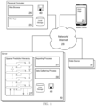
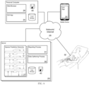
- FIG. 1 shows an example embodiment in which the system comprises one or more server devices [29] (each including eg a CPU processor circuit, memory, storage, GPU, FPGA etc) connected via a network/Internet connection [28] to one or more client devices, which may for example be a personal computer [33] or mobile device, and also to one or more data sources [32] (ie componentry which transforms or stores a record of some information of interest).
- the server device(s) execute program instructions from the stored program code [40], such that one or more Sparse Predictive Hierarchy [27] structures are constructed in memory, as well as a data gathering process componentry [30] and a reporting process componentry [31].
- the user interacts with the system using a mobile and/or a personal computer [33], which may have either a Graphical User Interface Application [25] or a web-based application [26], that may also be connected over a network/Internet connection [28].
- the Sparse Predictive Hierarchy [27] by learning to model the patterns of temporal evolution of the streams of signals from the data sources [32], is capable of detecting and signalling to the user, via the Graphical User Interface Application [25] on the client device, the presence of anomalous patterns in the measured data, allowing them to take appropriate action.
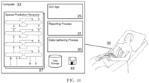
- FIG. 2 shows an Embodiment in which the system is contained in a single computer device (including eg a CPU processor circuit, memory, storage, GPU, FPGA etc), for example a personal computer [33], connected via a network/Internet connection [28] or other electronic signal communication to one or more data sources [32] (ie componentry which transforms or stores a record of some information of interest).
- the device executes program instructions from the stored program code [40], such that one or more Sparse Predictive Hierarchy [27] structures are constructed in memory, as well as a data gathering process componentry [30] and a reporting process componentry [31].
- the user interacts with the system using a Graphical User Interface Application [25] or a web-based application [26].
- the Sparse Predictive Hierarchy [27] by learning to model the patterns of temporal evolution of the streams of signals from the data sources [32], is capable of detecting and signalling to the user, via the Graphical User Interface Application [25], the presence of anomalous patterns in the measured data, allowing them to take appropriate action.
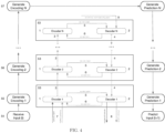
- FIG. 3 shows an arrangement of a typical embodiment of the Sparse Predictive Hierarchy.
- each processing stage [53] composed of a encoder [1] and a decoder [2] with encoder-decoder connection [5] and decoder-encoder connection [6], between them that enables the decoder [2] to predict the data coming from the encoder [1], also using its feedback connection [4], and the encoder [1] to represent the upcoming data from the feedforward connection [3] with the prediction errors of the decoder [2] via the decoder-encoder connection [6].
- the ladder is fed medical sensors and action input [7] and an optional top-down input [9], and produces a sensor prediction and chosen action output [8].
- FIG. 4 the succession of steps for encoding and prediction in a Sparse Predictive Hierarchy during a single timestep t are described in a flowchart, namely: receive input at timestep t [54] from the time-varying streams of data provided to the apparatus via the medical sensors and action input [7], generate encoding 1 [55] in the first processing stage [53] using this input (and previous values), generate encoding 2 [56] in the second processing stage using the encoding from the first processing stage [53], and so on until the N th processing stage will generate encoding N [57].
- the decoder of the N th processing stage will generate prediction N [58], which predicts the immediately next input value that will be received at the encoder of the N th processing stage at the next timestep. This prediction is sent to the decoder of the ( N - 1) th processing stage, where it is combined with the already-produced encoding for time t output by the corresponding encoder of the ( N - 1) th processing stage.
- the succession is continued at each i th processing stage, where a feedback prediction from the decoder of the ( i + 1) th processing stage is combined with the already-produced encoding for time t output by the corresponding encoder of the i th processing stage, and decoded to produce a prediction of the same encoder's input at an immediately next time step.
- the decoder of the second processing stage will generate prediction 2 [59] and provide this prediction to the decoder of the first processing stage, which will generate prediction 1 [60]. This prediction is used to predict the input at an immediately next timestep [61] of the Sparse Predictive Hierarchy.
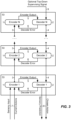
- FIG. 5 shows an arrangement of a typical embodiment of a single processing stage, which comprises Encoder/Decoder pair.
- the sensor and action input [7] multiplied by the feedforward weight matrix [10] to produce the stimulus vector [11].
- the previous activation [15] is combined with the stimulus vector [11] and cell biases [12] to update activation [16] values in the activation vector [17]. That is then fed through a top-k chooser [18] to produce a sparse activation [19], which is used to update states [20].
- the resulting states form the output of the encoder [1] which is passed up the feedforward connection [3].
- FIG. 5 further shows that the output from the encoder [1] is passed via the encoder-decoder connection [5] to the top of the decoder, where it is multiplied by the predictive weight matrix [22].
- the feedback signal from the feedback connection [4] is similarly multiplied by the feedback weight matrix [23], and the predictive and feedback signals are fed through a summation and a nonlinearity [24] to produce the decoder's sensor prediction and chosen action output [8].
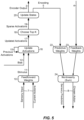
- FIG. 6 the succession of steps for learning in the Sparse Predictor encoder are described in a flowchart, namely: calculate prediction errors [34], calculate stimulus scale [35], calculate temporal difference [36] and multiply [37], update weights [38], and update biases [39].
- FIG. 7 shows an arrangement of a typical embodiment of a single Delay Encoder/Decoder pair.
- the sensor and action input [7] multiplied by the feedforward weight matrix [10] to produce the stimulus vector [11].
- the previous activation [15] is combined with the update activation [16], stimulus vector [11], and cell biases [12], to produce the activation vector [17]. That is then fed through a top-k chooser [18] to produce a sparse activation [19], which is used to update states [20].
- the resulting states form the output of the encoder [1] which is passed up the feedforward connection [3]. This output is further used to zero the firing activations [21] as those cells have already fired.
- FIG. 7 further shows that the output from the encoder [1] is passed via the encoder-decoder connection [5] to the top of the decoder, where it is multiplied by the predictive weight matrix [22].
- the feedback signal from the feedback connection [4] is similarly multiplied by the feedback weight matrix [23], and the predictive and feedback signals are fed through a summation and a nonlinearity [24] to produce the decoder's sensor prediction and chosen action output [8].
- FIG. 8 the succession of steps for learning in the Delay Encoder are described in a flowchart, namely: calculate feedforward traces [34], calculate importance matrix [35], calculate STDP matrix [36], calculate temporal direction [37], update weights [38], and update biases [39].
- a medical practitioner is concerned with the output from one or more medical sensors, in this example a heart monitor or Electrocardiograph (ECG).
- the heart monitor sensors are configured as data sources [32] and connected via a network/Internet connection [28] to one or more server devices [29], each of which contains at least one Sparse Predictive Hierarchy [27] as well as a data gathering process componentry [30] and a reporting process componentry [31].
- the user interacts with the system using a mobile and/or a personal computer [33], which may have either a Graphical User Interface Application [25] or a web-based application [26], that may also be connected over a network/Internet connection [28].
- the Sparse Predictive Hierarchy [27] by learning to model the patterns of temporal evolution of the streams of signals from the data sources [32], is capable of detecting and signalling to the user, via the Graphical User Interface Application [25], the presence of anomalous patterns in the measured heart, allowing the user and/or the medical practitioner to take appropriate action, such as providing appropriate treatment to prevent or mitigate harm to the patient.
- the user and patient are one and the same, and the entire system is contained in a mobile application (following the schematic of FIG. 10 ), connected to an ECG sensor array.
- the system is designed to provide an early-warning to the user/patient that anomalous patterns have been detected and that appropriate action should be taken.
- FIG. 11 shows an arrangement of a typical embodiment of the Routed Predictive Hierarchy Network.
- a series of layers each composed of an encoder [1] and a neural net layer [41] with preferable connections, encoder modulation connection [42] between them that enables the neural net layer [41] to form a subnetwork chosen by the data coming from the encoder [1], which modulates its inputs via the feedback connection [4], and the encoder [1] to represent the upcoming data from the feedforward connection [3].
- the hierarchy is fed medical sensors and action input [7] and an optional top-down input [9], and produces a sensor prediction and chosen action output [8].
- FIG. 12 depicts the cell components including activations, states, and connections in an example embodiment of a delay encoder module.
- FIG. 13 shows an arrangement of a distributed embodiment of the Sparse Predictive Hierarchy Network.
- the lower hierarchy [43] can operate in standalone mode or can be augmented by at least one upper hierarchy [44], which may be running in a server cluster or local PC's.
- the lower hierarchy [43] may be connected via a network/Internet connection [28] to the upper hierarchy [44] by one or both of the links depicted, namely the upward directed links [45] and downward directed links [46], which typically serve the same purpose as the feedforward connection [3] and feedback connection [4] respectively inside a Sparse Predictive Hierarchy Network. It may be seen that any number of devices may be connected in this manner to operate the distributed embodiment.
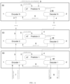
- FIG. 14 shows an arrangement of a typical embodiment of the Sparse Predictive Hierarchy Network with Time Division Feedback.
- a series of layers each composed of a encoder [1], a time division feedback predictor [47] and a decoder [2] with encoder-decoder connection [5] and decoder-encoder connection [6], between them that enables the decoder [2] to predict the data coming from the encoder [1], also using its feedback connection [4], and the encoder [1] to represent the upcoming data from the feedforward connection [3] with the prediction errors of the decoder [2] via the decoder-encoder connection [6].
- the hierarchy is fed medical sensors and action input [7] and an optional top-down input [9], and produces a sensor prediction and chosen action output [8].
- the time division feedback predictor [47] performs the transformation of the upper layer feedback output into the appropriate signal to combine with that from the same-layer encoder. In representation mode, this feedback signal is used to augment the representation produced by the encoder. In predictive coding mode, this feedback signal is used to correct the encoder's prediction signal. In either mode, the time division feedback predictor [47] feeds the decoder [2] with the feedback-corrected prediction [48] signal.
- the feedforward connection [3] and feedback connection [4] between each layer are each composed of n s connections, one for each lower layer timestep, thus requiring an equal number of weight matrices.
- the stimulus in each encoder is thus calculated by summing the stimuli for n s inputs together, and likewise the feedback connection [4] provides n s feedback signals to the lower layer, one for each of its timesteps.
- a stride of 2 or 3 is sufficient to ensure that many hundreds of bottom layer inputs are strided by layers only ten or so layers up.
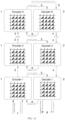
- FIG. 15 shows an schematic of a typical embodiment of the Chunk Encoder.
- Each chunk (four are shown) in the encoder has a visible receptive field [49] in its input layer, which is transformed by the chunk's local weight matrix [50], giving rise to a pattern of activation in the hidden chunk [51].
- the highest activated units in each chunk are chosen as the chunk winners [52], which are used as the encoding for the entire encoder.
- FIG. 16 shows an arrangement of a typical embodiment of the Sparse Predictive Hierarchy Network based on Memristor Crossbar Circuitry.
- FIG. 16 one sees a series of layers, each composed of a encoder [1] and a decoder [2] with encoder-decoder connection [5] and decoder-encoder connection [6], between them that enables the decoder [2] to predict the data coming from the encoder [1], also using its feedback connection [4], and the encoder [1] to represent the upcoming data from the feedforward connection [3] with the prediction errors of the decoder [2] via the decoder-encoder connection [6].
- the hierarchy is fed medical sensors and action input [7] and an optional top-down input [9], and produces a sensor prediction and chosen action output [8].
- the encoders and decoders using Memristor Crossbar Circuitry as depicted in FIG. 16 may be replaced by analog discrete circuits, digital differential analyser circuits, integrated ASIC circuitry (both analog and digital), FPGA circuitry, or any combinations thereof.
- Such circuits may be constructed so as to exactly correspond to the encoder/decoder designs as described elsewhere in the instant application, or as appropriate, they may use variations on such designs which take advantage of the properties of the hardware circuitry.
- each predictive hierarchy is constructed in the memory of the system as follows (for l layers, m in ⁇ n in inputs, and m out ⁇ n out outputs):
- Each sparse predictor contains a collection of visible and hidden layers indexed by i .
- Visible (input-facing) layers have size m vis i ⁇ n vis i
- hidden (output-facing) layers have size m hid i ⁇ n hid i .
- Each sparse predictor visible layer is constructed as follows:
- Each sparse predictor hidden layer is constructed as follows:
- the derived input D stores a copy of the immediate input x ij in d ij 1 , along with a moving average of past inputs in d ij 2 , and the temporal difference d ij 1 ⁇ d ij 2 is used in several places in the system.
- each sparse predictor is constructed with a "previous" copy of each 2D array and 4D weight matrix described above, denoted by a bar symbol, thus for example the previous activations are denoted A .
- the arrays and weight matrices are swapped, so for example A takes on the values of A , and A is either reset to zero or simply overwritten with new values during the processing.
- 3D matrices in place of 4D matrices as described herein.
- values may be calculated by ranging over a neighbourhood N ( ij , r ) of some position ( i , j) with a "radius" r.
- This neighbourhood ranges from i - r to i + r in one dimension, and from j - r to j + r in the other.
- the system calculates a "center" ( k 0 , l 0 ) in the second array corresponding to the position ( i , j ) in the first, and this is denoted as follows ( k 0 , l 0 ) ⁇ projection S ⁇ D ( i , j ). In this case the neighbourhood will be N ( k 0 , l 0 , r ).
- the window may or may not include the "center” element itself (eg inhibition ignores the center).
- simStep(inputs, learn) runs the hierarchy encoding and decoding passes, generates predictions and performs learning optionally.
- the upward pass involves feeding the encoders at each layer with the output of the lower layer encoder (or the input in the case of the bottom layer).
- the downward pass likewise involves running the decoders from top to bottom, processing top-down feedback from higher layers and the encoder output from the same layer.
- the prediction errors for each layer are then computed by comparing the predictions with the actual outputs and finally learning in the hierarchy updates the various weights and biases.
- the inputs here are shown as a single array of values for simplicity.
- the surrounding application or agent provides this input in each embodiment, so the structure and semantics of each input are application-dependent.
- the input may consist not only of medical sensory inputs such as video or image data, but may also include, for example, action selection information for a learning agent performing a task (e.g. in robotic applications).
- action selection information for a learning agent performing a task (e.g. in robotic applications).
- the output of the hierarchy may represent the choice of action the agent should take, along with its sensory prediction.
- the hierarchy may be configured to produce any desired form of output simply by specifying the size of the output of the bottom decoder.
- encodeHierarchy() passes input into the hierarchy, and run the up-pass for each layer.
- the input to the hierarchy may be preprocessed in some way (this is called whiten () in the example pseudocode below).
- whiten the encoder component processes the input, the encoder output states may then be optionally max-pooled (to add invariance), and the output is then passed up to the next higher layer.
- activateEncoder() and its kernels pass the hierarchy's inputs up from layer to layer. The input is first combined with its historical values to generate a derived input , and then converted into a stimulus which is the size and shape of the output encoding.
- the stimulus is combined with each unit's bias to produce the activation (which may include information about previous stimuli), and finally the usually sparse hidden states are computed as the output of the encoder stage.
- deriveInputKernel produces a pair of inputs for the encoder, one a copy of the input and the other a moving average of recent inputs.
- encodeKernel produces the encoder's stimulus, which is a weighted sum of each unit's derived inputs.
- the second element of the stimulus is a running sum of the squared norm of the weights used for each unit, which is used later to scale the encoder weight updates.
- the inputs on each connection are a kind of "delta" of the current input and the running average, as computed by the deriveInput function. This is merely one choice of input which is appropriate for many embodiments and tasks, but other choices may be used by the implementor.
- the stimulus in this example pseudocode is computed by a weighted sum of inputs over a neighbourhood of input units "centered" in the input array. This is one possible choice of computation, and it will be clear that other versions of such a computation may be used instead.
- the inputs to a unit may be randomly chosen from all inputs, or with a probability which varies with distance from the "center", and so on.
- activateKernel updates the hidden activations by combining the stimuli and biases.
- the stimulus is combined with the bias for each unit by addition, and then "temporally pooled" with the previous activation.
- This pooling allows activations to build up in a unit over a number of inputs, allowing for the activation to represent a temporal combination of a number of inputs in the past.
- solveHiddenKernel implements local inhibition on the activations to produce a sparse binary hidden state. First, each unit gathers information about its neighbours' relative levels, and then compares the number of more active neighbours with a threshold, only becoming active when the threshold is exceeded.
- the example pseudocode implements a local inhibition process over a neighbourhood N ( ij , r ) of a unit, and imposes a local sparsity level which is a parameter for the encoder. This will be seen as one choice among several which may be used to control the number of active or firing units in the encoding. For example, an embodiment may use a global inhibition process which ignores the positions of the most active units and simply chooses the top k activations among all units.
- this pseudocode produces a sparse binary encoding, but some embodiments or implementors may employ other, non-binary encodings, such as for example employing a rectified linear unit (ReLU) to produce a sparse continuous output.
- ReLU rectified linear unit
- some embodiments may impose a "refractory period" on active states, for example by not allowing a unit to become active if it was active in the previous step (or in some number of previous steps). In such a case, the units will be prevented from remaining active too much, creating a kind of temporal sparsity in the encoding.
- Other similar methods might involve maintaining a decaying trace of previous firing and thus smoothly inhibit the reactivation of a unit.
- this temporal feedback inhibition may employ the process of setting the corresponding activation value of a unit to zero if it fires in the current timestep (as used in the Delay Encoder described elsewhere).
- Another class of encoder embodiments may perform other versions of processes to generate the encoding.
- One such example is an iterative solver, which cycles over a number of substeps for each timestep, performing recurrent inhibition over the activations as they are accumulated, counting the number of times each unit fires during the timestep, and using that to perform inhibition and generate the states.
- maxPoolKernel creates a summarised representation of the hidden state.
- Decoding information passes down the hierarchy, as each layer generates predictions by decoding its encoder's output, combined with feedback from higher layer decoder predictions.
- the feedback input Z fb is either the higher layer decoder output or the current hidden state in the case of the top layer.
- the decoder produces two predictions, one based on the feedback and the other, lateral prediction, on the corresponding encoder hidden state. These predictions are combined to produce the decoder's output.
- the decoder will use other inputs besides the (usually binary) hidden encoder states and higher layer decoder outputs.
- the activation values used in the encoder may be used instead, since they contain more of the distributed information passing up the hierarchy.
- decodeKernel transforms either the hidden or feedback inputs to the decoder using a weight matrix, forming a partial prediction.
- the above example pseodocode uses a weighted sum over a centered neighbourhood to compute the decoder's prediction for an output unit.
- This choice (which we denote as a "Linear Decoder") is one among many as mentioned earlier.
- combinePredKernel blends the feedback and lateral predictions to produce a continuous (typically for the output decoder) or optionally locally sparse prediction output from the decoder.
- the above example pseudocode provides two options for the decoding, one of which is continuous-valued across the prediction, and the other which is sparse and binary. This is designed to allow the output to match the properties of the corresponding encoder's input (which will often be continuous for the bottom layer and sparse for upper layers). Clearly this is just one choice for producing an appropriate prediction, and variations may be employed as the task demands.
- the decoding to a sparse prediction described in the example pseudocode above uses local inhibition in similar manner to the encoder described above. Similarly, variations on this choice of imposition of sparsity may be used for the decoder's prediction.
- Prediction Errors are used in the hierarchy to drive local learning, both in the encoder and decoder.
- a target is computed, and compared with the prediction to generate a raw prediction error E Y in the input space of each layer. This is then used to compute an encoder hidden state error E Z which is an estimate of the errors in the encoder output.
- propagateErrors reverses the decoding transformation to derive the errors in the encoder hidden states.
- This example pseudocode effectively reverses the decoder's processing of lateral encoder outputs, in order to generate an error vector in the encoding space. It uses a process which is analogous to that used in decodeKernel , namely weighted sums over neighbourhoods, using the same encoding matrix W lat (transposed). This reverse process may be varied as appropriate to correspond to that used in the forward version.
- Learning in the hierarchy involves using the prediction errors and the decoder inputs (hidden states or feedback) to update decoder weights, and a Spike-time Dependent Plasticity (STDP)-like rule to update the encoding weights.
- learnDecoder updates the decoder weights by combining the prediction error on the output with the input to that weighted connection.
- learnEncoder uses a STDP-like mechanism to update the encoder weights, combining the hidden errors, the hidden state, and the derived inputs at each end of the weight's connection.
- the second component of the weights tensor is a trace of past correlations of hidden states and inputs.
- the factor scale uses the second component of the stimulus tensor, which is the squared norm of the incoming encoder weights.
- the biases may be updated in several manners, in a way such that the states of a unit have a desired lifetime sparsity.
- One such method is to updated the biases such that the average stimulus received by a unit approaches zero.
- the above learning rules represent a typical embodiment. Depending on the task, other embodiments may adapt these rules or use alternative rules.
- the pseudocode is provided only as an example, and a reader skilled in the art will understand that the system can be implemented in any modern computer language, depending on the platform and performance characteristics of relevance. For example, the system has been built and operated in C++, Go and Java as well as Python, and run on CPU and CPU/GPU systems.
- the following describes another class of embodiment of the invention, which is denoted as a Routed Predictive Hierarchy.
- This variation differs from the aforementioned in that encoders and decoders interact through modulation as opposed to error propagation.
- the encoders in what follows are trained separately from the decoding phase, and the decoding phase consists of a decoder network whose states are modulated by the encoders. This causes the encoders to choose sub-networks for the decoder network, simplifying training and more importantly adding spatiotemporal context to predictions.
- simStep(inputs, learn) runs the hierarchy encoding and decoding passes, generates predictions and performs learning optionally.
- encode() pass input into the hierarchy, and runs the up-pass for each layer.
- deriveInputKernel produces a pair of inputs to the encoder, one a copy of the input and the other a moving average of recent inputs.
- encodeKernel produces the encoder's stimulus, which is a weighted sum of each unit's derived inputs.
- solveHiddenKernel implements local inhibition on the activations to produce a sparse binary hidden state.
- hierarchyPredict() The previously stated algorithms comprise the encoder section of the Routed Predictive Hierarchy. The prediction is handled by a standard feed-forward deep neural network, with the caveat that the activations are modulated by the states of the encoder portion of the system.
- This prediction network is trained via backpropagation or other means while taking into account the modulating states Z from the encoder hierarchy.
- This modulation forms subnetworks of the predictor network that are specific to a spatiotemporal state, allowing for improved generalization capabilities as well as fast online training.
- the predictor network can be a linear function approximator, simplifying the credit assignment problem due to lack of a vanishing gradient.
- An example embodiment is one which uses for decoding a standard feed-forward deep neural network operated upside down (from upper layers towards the input layer). The following describes how decoding is performed in this embodiment.
- Decoding information passes down the hierarchy, as each layer generates predictions by decoding its input from higher layer decoder predictions, modulated by its encoder's hidden states (ie z ij mod ⁇ z ij ⁇ b z ij ).
- decodeKernel transforms the modulated feedback inputs to the decoder using a weight matrix, adding biases, and forming a partial prediction via an optional nonlinearity (defaults to the identity function).
- hierarchyLearn runs the learning for each layer's encoder.
- the Routed Predictive Hierarchy in particular is well-suited to reinforcement learning due to the ease of combining additional networks through state modulation.
- the Routed Predictive Hierarchy may be incorporated in a reinforcement learning focused embodiment by using the encoder hierarchy to modulate a collection (or "swarm") of small reinforcement learning agents.
- Each visible state is paired with a small reinforcement learning agent whose actions are modulated by the encoders.
- each spatiotemporal state creates a different ensemble of small reinforcement learning agents.
- the agents produce actions which are either treated as action outputs, or are fed in as input to the next lower layer agents. This creates a form of hierarchical reinforcement learning.
- Such reinforcement learners as with a prediction network, are trained online with the help of the modulatory encoder hidden states. This also allows one to easily use eligibility traces to improve learning speed.
- the underlying algorithm behind each agent in the ensemble can vary between implementations as well as within individual layers in order to better encompass the task at hand.
- a simpler but more limited embodiment uses an encoder-modulated feed forward backpropagation network to learn Q values for different actions.
- this method doesn't readily exploit hierarchical action selection or continuous (or discrete approximations of continuous) actions. Though less powerful, it may be more suitable if the surrounding apparatus requires such a design.
- Routed Predictive Hierarchy may be used not only in the various embodiments and configurations described herein, but in combination with and acting as a spatiotemporally-aware controller and modulator for learning systems of any kind.
- the operation of a system based on the Sparse Predictive Hierarchy or Routed Predictive Hierarchy may, as previously described, be enhanced for certain tasks by replacing some encoder/decoder modules with encoder/decoder variants which are more suitable for the task.
- encoder/decoder variants which are more suitable for the task.
- the first variant module is denoted the Binary Iterative Shrinkage-Thresholding Algorithm (BISTA) encoder. It learns to produce a sparse binary code for a high-dimensional continuous-valued bottom-layer input which can be directly decoded by the decoder component. This provides sparse codes for higher layers, at the cost of some iteration in the bottom layer only.
- BISTA Binary Iterative Shrinkage-Thresholding Algorithm
- the second variant module is called the Spike Propagation (SpikeProp) encoder. It is a variation on the Delay Encoder as described above. As will be described, the SpikeProp encoder uses the actual sparse binary input (usually from a lower encoder), backpropagated through the decoder transformation, to produce a target spike pattern for the encoder hidden layer, and this target is used to drive STDP learning instead of the actual hidden output (and transformed prediction error) as used in the Delay Encoder described earlier.
- SpikeProp uses the actual sparse binary input (usually from a lower encoder), backpropagated through the decoder transformation, to produce a target spike pattern for the encoder hidden layer, and this target is used to drive STDP learning instead of the actual hidden output (and transformed prediction error) as used in the Delay Encoder described earlier.
- the BISTA encoder activate() and its kernels pass the hierarchy's inputs up from layer to layer. Each step around the iterative solver, the previous spike pattern is used to generate a reconstruction of the input.
- the reconstruction error E recon forms the input to generate new stimuli S , which are then used to generate activations A, and those are inhibited to generate the new spike pattern.
- derivelnputKernel produces a pair of inputs to the encoder, one a copy of the input and the other a moving average of recent inputs.
- reverseKernel calculates the current reconstruction error given the current hidden solution and the derived inputs.
- encodeKernel produces the encoder's stimulus, which is a weighted sum of each unit's input reconstruction errors.
- activateKernel produces the encoder's activations from the stimulus.
- solveHiddenKernel implements local inhibition on the activations to produce a sparse binary hidden state.
- the result of the iterative solving is a sparse code which represents a number of steps towards the minimisation of reconstruction errors of the encoder.
- the remainder of the hierarchy uses the SpikeProp encoders.
- encodeHierarchy() pass input into the hierarchy, and run the up-pass for each layer.
- the BISTA layer converts the inputs into a sparse binary hidden state, and then each successive layer builds its representation.
- the activateEncoder() and its kernels pass the hierarchy's inputs up from layer to layer.
- the encoding and decoding are combined.
- deriveInputKernel produces a pair of inputs to the encoder, one a copy of the input and the other a moving average of recent inputs.
- encodeKernel produces the encoder's stimulus, which is a weighted sum of each unit's derived inputs.
- activateKernel produces the encoder's activations from the stimulus, the previous activations, and the previous states. The activation is constrained non-negative by a Rectified Linear Unit. solveHiddenKernel implements local inhibition on the activations to produce a sparse binary hidden state.
- decodeKernel transforms the hidden inputs to the decoder using a weight matrix, forming a partial prediction. hierarchyLearn runs the learning for each layer's encoder. propagatelnputs reverses the decoding transformation to derive the stimulus for spike propagation. stimulusKernel computes the stimulus due to the raw inputs.
- learnEncoder uses a STDP-like mechanism to update the encoder weights, using the hidden state due to the input at each end of the weight's connection. learnDecoder updates lateral weights.
- each delay encoder is constructed in the memory of the system as follows (for m inputs and n outputs):
- ⁇ refers to elementwise multiplication of same-sized vectors or matrices; ⁇ refers to an outer product of arbitrary vectors, forming a matrix result.
- J n is an n-dimensional vector of all 1's, and J n,m is an n ⁇ m- dimensional matrix of all I's.
- W i is the i th row of matrix W .
- Example code (in Python) for activation is as follows:
- T t ⁇ T t ⁇ 1 ⁇ J n , m ⁇ Z t ⁇ 1 + X t ⁇ 1
- Example code (in Python) for learning is as follows:
- the above learning rules represent a typical embodiment. Depending on the task, other embodiments may adapt these rules or use alternative rules.
- the Python code is provided only as an example, and a reader skilled in the art will understand that the system can be implemented in any modern computer language, depending on the platform and performance characteristics of relevance. For example, the system has been built and operated in C++ and Go as well as Python, and run on CPU and CPU/GPU systems.
- STDP spike time dependent plasticity
- the activation update can be modified to remove the non-linearity (max): a ij ⁇ ⁇ a a ⁇ ij 1 ⁇ z ⁇ ij + 1 ⁇ ⁇ a s ij which results in an activation that is bounded to s ij through a running average with its own decay rate ⁇ a .
- the Chunk Encoder is an improved piece of componentry which may be used as a replacement for other encoders in the Predictive Hierarchy as described elsewhere in the instant application.
- the Chunk Encoder splits its output hidden state layer into small tiles called chunks, which operate as small, semi-independent self-organising representers of the underlying input data. Each chunk chooses a winning cell by inhibition for each timestep, and the weights in the chunk's units are updated to try to follow the winner for the given input.
- activate and its kernels pass the hierarchy's inputs up from layer to layer.
- the input is first combined with its historical values to generate a derived input, and then converted into a stimulus which is the size and shape of the output encoding.
- the stimulus is combined with each unit's bias to produce the activation (which may include information about previous stimuli), and finally the usually sparse hidden states are computed as the output of the encoder stage.
- Listing 1 sfcDerivelnputs transforms the input into a delta of the input and previous trace, and a new trace value, a running average of previous inputs.
- Listing 2 sfcAddSample makes a shifted copy of the samples tensor samplesBack and adds the new input from visibleState at index 0, placing the result in samplesFront.
- Listing 3 sfcStimulus computes the stimulus hiddenSummationTempFront by taking a window of inputs from visibleStates, subtracting a weight (taken from weights) from each input, and summing the squares.
- Listing 4 sfcActivate calculates the activations by adding the stimulus to the bias for each unit.
- Listing 5 sfcInhibit performs chunk-wise inhibition for each activation
- Listing 6 sfcInhibitOther performs chunk-wise inhibition on the encoder output states.
- Listing 7 sfcReconstruct forms a prediction from the encoder hidden states, using a linear transformation. learn runs the learning kernel sfcLearnWeights in the Chunk Encoder. The learning mechanism operates on each chunk of hidden states, using the chunk winner as a target for each weight leading into a hidden unit.
- sfsLearnWeights is an alternative learning process for previous encoders as detailed earlier.
- the learning uses a variant of Spike Time Dependent Plasticity, as before, but in this case the delta ⁇ stdp is (minus) the product of the previous state z kl and the change in the input ( d ij - d ij ) .
- Listing 10 sfsLearnWeights uses an improved STDP learning rule for the Delay Encoder.
- fhPool performs max-pooling over time (MPoT) to slow changes passed up the hierarchy. This has the effect of allowing higher layers to learn longer-range features of the input stream and thus provide higher-level context to assist lower layers in prediction.
- This kernel is run at the end of the Encoder's activate step as described earlier.
- Listing 11 fhPool performs max-pooling over time (MPoT) to slow changes passed up the hierarchy.
- encoders are shown and described, such as delay encoders and chunk encoders, one should appreciate that these are merely examples. Other types of encoders may be used, provided they generate nonlinear encodings at their outputs that are based upon both current inputs and previous inputs.
- the words “comprising,” “including,” “containing,” and “having” are intended to set forth certain items, steps, elements, or aspects of something in an open-ended fashion.
- the word “set” means one or more of something. This is the case regardless of whether the phrase “set of” is followed by a singular or plural object and regardless of whether it is conjugated with a singular or plural verb.
- ordinal expressions such as “first,” “second,” “third,” and so on, may be used as adjectives herein, such ordinal expressions are used for identification purposes and, unless specifically indicated, are not intended to imply any ordering or sequence.
- a "second” event may take place before or after a "first event,” or even if no first event ever occurs.
- an identification herein of a particular element, feature, or act as being a “first” such element, feature, or act should not be construed as requiring that there must also be a "second” or other such element, feature or act. Rather, the "first” item may be the only one.
Landscapes
- Engineering & Computer Science (AREA)
- Theoretical Computer Science (AREA)
- Physics & Mathematics (AREA)
- Software Systems (AREA)
- Artificial Intelligence (AREA)
- Data Mining & Analysis (AREA)
- Evolutionary Computation (AREA)
- Computing Systems (AREA)
- General Engineering & Computer Science (AREA)
- General Physics & Mathematics (AREA)
- Mathematical Physics (AREA)
- Computational Linguistics (AREA)
- Life Sciences & Earth Sciences (AREA)
- Health & Medical Sciences (AREA)
- Biomedical Technology (AREA)
- Biophysics (AREA)
- General Health & Medical Sciences (AREA)
- Molecular Biology (AREA)
- Medical Informatics (AREA)
- Computer Vision & Pattern Recognition (AREA)
- Neurology (AREA)
- Compression Or Coding Systems Of Tv Signals (AREA)
- Image Analysis (AREA)
Description
- This applications claims the benefit of the filing date of the following provisional patent applications:
U.S. Application No. 62/341,790, filed May 26, 2016 U.S. Application No. 62/382,992, filed September 2, 2016 U.S. Application No. 62/424,226, filed November 18, 2016 U.S. Application No. 62/464,090, filed February 27, 2017 - The present invention relates generally to computerized technology for processing temporal sequences of data, and, more particularly, to computerized techniques for efficiently processing and predicting such sequences.
- Many applications in industry, consumer devices and healthcare involve the processing and transformation of raw information signals into useful or improved outputs which can be interpreted by users or passed on for further analysis, processing and decision making. These signals are often both high-dimensional and high-velocity, for example vehicle camera video, Magnetoencephalograph (MEG), and sensors embedded in large machines.
- Such applications traditionally require the manufacturer to develop complex hardware and software systems in order to process the raw inputs from sensors and generate outputs which are valuable to the user. This incurs significant research, development, testing and maintenance costs, which adds to the expense and running costs of the system. This is exacerbated by the need to largely rewrite or re-engineer such systems when new components are added, the sensor technology changes, or the system is repurposed for a new application domain.
- Traditional systems of this kind also usually require the employment of experts at every stage, from the identifying of requirements, to vendor selection and purchasing, installation, integration, maintenance and most importantly operation. Such experts may be rare and costly, and are diverted from other productive tasks in an organisation. All this complication and cost reduces the scale at which new analytical and diagnostic systems can be adopted, and thus significantly reduces the benefits available to industry, consumers and health practitioners of advances in sensor technology.
- In answer to this, some progress has been made by using machine learning to replace or augment traditional hand-engineered and hand-coded componentry in such systems. Unfortunately, most such machine learning methods are ill-suited to the particular conditions which exist in the domains under discussion, for a variety of reasons. Examples for machine learning approaches are known e.g. from Pezeshki et al., Deconstructing the ladder network architecture; axXiv: 1511.06430v4 and Rasmus et al., Semi-supervised learning with ladder networks, arXiv: 1507.02672v2.
- First, such systems themselves require high expertise in both the configuration of the learning system and its application to the type of data of interest. Such expertise may be unavailable or in short supply, and in any case will be expensive.
- Second, most machine learning systems are trained in a supervised manner, which requires a very large amount of previously prepared labelled data which acts as a target. Producing labelled data is often an expensive process which itself requires significant expertise. When the training is complete, such systems may have to work on data which differs significantly from that found in the training set, and indeed may change from time to time, from machine to machine or from patient to patient.
- Third, most machine learning methods either ignore temporal structure completely, or else treat it only as a dimension of finite extent. Many processes in industry, medicine and the outside world are very complex dynamical systems, where correlation-based strategies might not be appropriate, and so the ability to model the data temporally and dynamically is of crucial importance.
- Finally, most such methods often have very high computational costs in terms of processor speed, power consumption, and memory, and often need high-end Graphical Processing Units (GPUs), or even clusters of them, to perform training and/or inference. Such systems may be infeasible or impossible in many applications, and in any case will add significantly to their purchase, installation and running costs.
- The invention is set out in the appended set of claims.
- For a more complete understanding of the invention, reference is made to the following description and accompanying drawings, in which:
-
FIG. 1 is a block diagram of an example network arrangement in which embodiments of the invention can be practiced; -
FIG. 2 is a block diagram of an example single-machine arrangement in which embodiments of the invention can be practiced; -
FIG. 3 is a block diagram of an example Sparse Predictive Hierarchy Network, which may be suitable for use in the arrangements ofFIGS. 1 and2 ; -
FIG. 4 is a flowchart showing an example method performed by the Sparse Predictive Hierarchy Network ofFIG. 3 ; -
FIG. 5 is a block diagram showing an example Encoder/Decoder pair, which may be employed in the Sparse Predictive Hierarchy Network ofFIGS. 3 and4 ; -
FIG. 6 is a flowchart showing an example method of encoder learning; -
FIG. 7 is a block diagram of an example Delay Encoder/Linear Decoder pair; -
FIG. 8 is a flowchart showing an example method for delay encoder learning; -
FIG. 9 is a block diagram showing an example network arrangement in which the Sparse Predictive Hierarchy Network ofFIGS. 3 and4 may be employed in an Electrocardiograph (ECG) measurement system; -
FIG. 10 is a block diagram showing an example single-machine arrangement in which the Sparse Predictive Hierarchy Network ofFIGS. 3 and4 may be employed in an Electrocardiograph (ECG) measurement system; -
FIG. 11 is a block diagram of an example Routed Predictive Hierarchy Network; -
FIG. 12 is a schematic diagram showing production of delay encoder states; -
FIG. 13 is a block diagram of an example Distributed Sparse Predictive Hierarchy; -
FIG. 14 is a block diagram of an example of a Time Division Feedback Sparse Predictive Hierarchy; -
FIG. 15 is a perspective view of an example tiled Chunk Encoder; and -
FIG. 16 is a schematic diagram of an example Sparse Predictive Hierarchy based on Memristor Crossbars. - Embodiments will now be described with reference to the figures. It will be appreciated that for simplicity and clarity of illustration, where considered appropriate, reference numerals may be repeated among the figures to indicate corresponding or analogous elements. In addition, numerous specific details are set forth in order to provide a thorough understanding of the embodiments described herein. However, it will be understood by those of ordinary skill in the art that the embodiments described herein may be practiced without these specific details. In other instances, well-known methods, procedures and components have not been described in detail so as not to obscure the embodiments described herein. Also, the description is not to be considered as limiting the scope of the embodiments described herein.
- It will also be appreciated that any module, unit, component, server, computer, terminal or device exemplified herein that executes instructions may include or otherwise have access to computer readable media such as storage media, computer storage media, or data storage devices (removable and/or non-removable) such as, for example, magnetic disks, optical disks, or tape. Computer storage media may include volatile and non-volatile, removable and non-removable media implemented in any method or technology for storage of information, such as computer readable instructions, data structures, program modules, or other data. Examples of computer storage media include RAM, ROM, EEPROM, flash memory or other memory technology, CD-ROM, digital versatile disks (DVD) or other optical storage, magnetic cassettes, magnetic tape, magnetic disk storage or other magnetic storage devices, or any other medium which can be used to store the desired information and which can be accessed by an application, module, or both. Any such computer storage media may be part of the device or accessible or connectable thereto. Any application or module herein described may be implemented using computer readable executable instructions that may be stored or otherwise held by such computer readable media.
- The following describes in detail the construction of appropriate networks, the structure of several module designs and the transformations they perform, the processes involving the signalling between modules, and the steps involved in learning in the modules.
- In the following, a "frame" of data is the term used for any amount of data (not limited to image frames) which is presented to the system at any given moment, and a "stream" or "flow" or "sequence" or "signal" of data is a series of successive frames of data which are each recorded or received at the same time (or close together in time), or stored together in a storage medium. For example, a video camera may produce a sequence of image frames, 30 per second, and such a sequence may be stored in a computer file or on a digital tape.
- An "encoder" is a piece of componentry which transforms each frame of data in one form into another form, possibly in combination with other frames from the same stream, and also with other data. The frame of data produced by an encoder is usually called the "encoding" of the input frame or frames.
- Conversely, a "decoder" is a piece of componentry which transforms a frame of data in the language or form of an encoding back into a form similar to that expected as input to an encoder. For example, an encoder for video might take frames of pixel color values and transform them into a compressed form for storage and transmission, and a decoder might later take such a compressed file and decode it into a form suitable for display.
- A "sparse encoding" is a frame of numeric data where most values are zero and only some are non-zero. A "binary sparse encoding" is one where the non-zero values are all equal to one.
- Several terms appear in the following which are used conventionally in machine learning and neural networks, for example "hidden" and "visible" layers and units, "feedforward", "feedback" and "recurrent", "activation", "weight" etc. These terms will be recognised by those skilled in the art to have their usual meanings.
- As found conventionally in machine learning and neural networks, collections or arrays of scalar values may be referred to herein as "layers" of "units". When a component (encoder or decoder) has several layers of the same dimensions, each vector of scalar values in the same position in the several layers is referred to as a "cell."
- An innovation of the invention, the "Predictive Hierarchy", is part of the componentry in the apparatus. The predictive hierarchy comprises a stack of "processing stages", each processing stage including a paired encoder and decoder. The processing stages form autoencoder-like "layers," in which feedforward signals are fed up the hierarchy in a chain of encoder modules, feedback and predictive signals are passed down the hierarchy via a chain of decoders, and recurrent connections across and between layers allow for learning and prediction assistance at both the local and network levels.
- The succession of steps for encoding and prediction in a Sparse Predictive Hierarchy during a single timestep t are described as follows: receive input at timestep t from the time-varying stream of data provided to the apparatus via the sensor and action input, generate encoding 1 in the first processing stage using this input (and previous values), generate encoding 2 in the second processing stage using the encoding from the first processing stage, and so on until the Nth processing stage will generate encoding N. Using the resulting encoding, the decoder of the Nth processing stage will generate prediction N, which predicts the immediately next input value that will be received at the encoder of the Nth processing stage at the next timestep. This prediction is sent to the decoder of the (N - 1) th processing stage, where it is combined with the already-produced encoding for time t output by the corresponding encoder of the (N - 1) th processing stage. The succession is continued at each ith processing stage, where a feedback prediction from the decoder of the (i + 1) th processing stage is combined with the already-produced encoding for time t output by the corresponding encoder of the ith processing stage, and decoded to produce a prediction of the same encoder's input at the next time step. Finally, the decoder of the second processing stage will generate
prediction 2 and provide this prediction to the decoder of the first processing stage, which will generateprediction 1. This prediction will be used to predict the immediately next input value at the next timestep of the Sparse Predictive Hierarchy. - Each predictive hierarchy processing stage, by virtue of its recurrent and lateral connections, is capable of locally and independently processing its inputs and generating both spatiotemporal encodings and predictions of future inputs, thus learning a spatiotemporal model of its (feedforward and feedback) sensorimotor world.
- Simply by stacking processing stages in the predictive hierarchy, the hierarchical spatiotemporal structure in real world data is modelled in the structure of the network, so learning and prediction is enhanced in each layer.
- Due to the self-contained processing power of each predictive hierarchy processing stage and the small size of sparse encodings, the predictive hierarchy network can be very easily distributed across heterogeneous computing devices connected by low-bandwidth links. For example, low-power devices running the lower processing stages of the hierarchy may be dynamically augmented by adding higher processing stages running on more powerful cloud infrastructure. This design is robust to network outages, as all connected processing stages at the bottom of the hierarchy will continue to function in a graceful degradation.
- Due to its modular nature, involving a uniform Application Programming Interface (API) for encoders, decoders, and the communication between them, the implementer of a predictive hierarchy system can replace any particular processing stage described herein with variants or complete replacements conforming to their needs.
- Replacing modules is described herein, where a continuous high-dimensional input is encoded to sparse binary form in the first processing stage by an iterative solver module, and the upper layers consist of encoders based on a spike propagating ("SpikeProp") variation of the Delay Encoder described below.
- The effect of the lateral connections between encoder and decoder may also be varied by the implementer of a predictive hierarchy system. For example we describe two embodiments of what are denoted Routed Predictive Hierarchies, in which the encoders control the activity of feedforward neural networks in the first, and swarms of reinforcement learning agents in the second. It will be clear to those skilled in the art that the improvements provided by the predictive hierarchy may easily be thus incorporated into existing machine learning or control systems.
- Due to its uniform API, the predictive hierarchy itself is a component which may be used in various ways in different embodiment. For example, we detail embodiments which predict the immediately next input value of the input data streams.
- The present invention is designed to be easily re-implemented in any modern programming language and on all kinds of hardware, including single-core or multi-core Central Processing Unit (CPU), Graphical Processing Unit (GPU), Field Programmable Gate Array (FPGA) etc. In addition, example embodiments are described in which an entire system runs on a single device, in which a system is distributed across multiple devices, in which a network of systems is formed, and in which a system can be dynamically augmented with extra processing stages.
- The encoders and decoders in the predictive hierarchy may, furthermore, be implemented using hardware circuitry, both traditional analog and digital, discrete and integrated, and also using non-traditional circuitry such as neuromorphic and memcomputing circuitry.
- Due to the uniform structure of the internal learned model data, separate instances of the present invention may communicate their internal memory structures using a standard buffer library. For example, this allows pretraining of a system using high-performance server clusters for eventual deployment on a low-power, mobile or embedded device where compute power or data transmission for training is infeasible. It also allows devices to perform backup and recovery of learned models in case of failure or error. Further, it allows redeployment of systems from a single device to a cluster, from a cluster of one size to one of another, and so on, as the operator requires.
- An embodiment of the present invention is capable of immediate online learning and predictive performance without pretraining or supervision of any kind, the performance improving as it continues to learn the data. In addition, the system may, depending on its settings, continuously adapt to any trending changes in the characteristics of the data. Further, we detail embodiments which use the system in a fully- and weakly- or semi-supervised regime, as well as reinforcement learning.
- One class of embodiments of the present invention comprises one or more server devices (which e.g. include CPU processor circuitry, computer memory, persistent storage, GPU and/or FPGA circuitry etc), loading and executing a stored program code which implements the componentry described herein, and connected to a device which is a source of temporal data signals (e.g. toencephalograph (MEG) sensors), or to storage which contains a recording of said data. The input data is used by the apparatus to automatically learn about the spatial and temporal structure of a problem and to form predictions. The apparatus then provides the user with information relevant to a task which is derived from these predictions and anomalies.
- In a typical example embodiment, each encoder module consists of an optional input transformer (usually a linear transformation), and a globally or locally connected weight matrix, which transforms the derived inputs into a stimulus layer.
- The encoder module may in some embodiments combine its companion decoder's predictions (or their prediction errors) with its own inputs, either by merging or by concatenation, depending on the embodiment. In addition, feedback from higher layers may similarly be combined, either raw or with some preprocessing, with the feedforward stimulus as drawn from the weight matrix.
- To incorporate temporal structure in the encoder representations, inputs, stimuli and activations may all be formed with respect to their own histories in various ways described herein, and the overall performance of each processing stage, as measured by prediction errors, may be used to guide the updates of the encoder and decoder weight matrices.
- An innovation of the invention, the "Delay Encoder", is part of the componentry in the apparatus in some embodiments. Each delay encoder comprises an autoencoder-like two-layer architecture, containing a "visible" (input) layer and a "hidden" (output) layer. The hidden layer is connected to the input layer through a set of synapse-like weighted connections. Each connection contains two values: A weight, and an eligibility trace. These connections feed into the array of hidden layer "cells," which can be of a different dimension. Each cell contains four variables: the "stimulus," "activation," "trace," and (output) "state." Together these variables form a sort of time-keeping system. In addition to those time-keeping variables, each cell also has a homeostatic regulation variable (bias). Finally, each input also has an associated trace, which can simply be the cell trace if the input corresponds to a cell from another layer.
- The delay encoder layer first computes the stimulus of the hidden cells using a matrix multiplication, or simply multiplying each input by its corresponding weight. This step is similar to the operation of standard feed-forward neural networks and autoencoders.
- Having computed the stimulus, the encoder adds it to the current activation value of each cell, and subtracts the cell bias. This means that the activation either increases or decreases with each stimulus. Some embodiments may constrain the activations to only be positive.
- Finally, the encoder sets the output cell states to 1 for the top K highest-activation cells, where K is the target sparsity level, while the rest of the output states are set to 0. Once a cell's state is 1 (which is referred to as a spike), its activation is reset to 0.
- This example method of operation is a simplified version of standard spiking neurons, but with an important difference: Neurons only fire and reset their activations when they are part of the top K highest activations. This can be thought of as implementing a sort of neural stack, where the top K elements are popped from every simulation tick. This distinction allows cells to remain unaltered by the state of other cells until it is their "turn" to fire, and cells cannot fire on their own, they must be higher than some percentage of the population of cells.
- In a typical embodiment, a delay encoder learns using a novel spike-timing dependent plasticity (STDP) based learning rule. Each connection in the delay encoder computes a STDP function that indicates the preferred temporal direction the connection would like the corresponding cell to take. The STDP values of all connections are averaged together to get the total temporal direction the cell should move in order to maximize the number of inputs the cell is predicting. Using this direction vector, each cell can be updated to fire either sooner or later depending on the desired temporal direction. This is done by maintaining another set of per-connection traces, which accumulate inputs and are reset to 0 when the cell emits a spike. The final update to the connection weights is then a product of the desired temporal direction and the eligibility trace for a connection.
- To make sure the system doesn't diverge, the encoder includes for each cell a homeostatic regulatory variable - its bias. As aforementioned, the bias is an additional value subtracted from the activation of a cell in each simulation tick. It is updated to make sure that the total stimulus of a cell is on average 0.
- We assume that a decoder (which, in typical embodiments, is a simple linear combination of the hidden states of the encoder) provides predictions from each encoder by using the standard perceptron learning rule with a time delay. In some embodiments, this decoder solely provides predictions from the encoder hidden state, and can feed back in to the encoder (as when using the previously described STDP-based learning rule for the encoder). In other embodiments the connection is used to provide additional information to the delay encoder about decoder prediction errors.
- A single delay encoder (paired with an appropriate decoder) can learn complex sequences on its own, but the complexity of the system can be reduced (improved) by adopting a hierarchical approach. The idea is to simply stack several delay encoders, where the input layer of one encoder is either the input to the whole system or the hidden layer (output) of a lower delay encoder. The decoders then go in the opposite direction, each generating a prediction of the next hidden state of its corresponding delay encoder using information from the paired encoder and higher-layer encoders or decoders.
- In a typical embodiment, the activation phase of the system is separated into two phases to improve performance with respect to computational resources. One can first perform an upwards-pass that activates all delay encoders in order, and then a downwards-pass that activates all decoders in order while referencing the encoders. This avoids iterative solving for a dynamical system.
- The STDP portion of the learning rule is assumed to be the standard temporal association STDP learning rule (excitatory STDP). However, it is vital for the delay encoder that these STDP values do not directly update the connection weights as in most literature, but rather that they are averaged (possibly with weighting) to determine the cell's temporal direction, where the direction then modulates a set of per-connection eligibility traces in order to update the connection weights.
- The "Chunk Encoder" is an improved piece of componentry which may be used as a replacement for other encoders in the Predictive Hierarchy as described elsewhere. The Chunk Encoder splits its output hidden state layer into small tiles called "chunks," which operate as small, semi-independent self-organising representers of the underlying input data. Each chunk chooses a winning cell by inhibition for each timestep, and the weights in the chunk's units are updated to try to follow the winner for the given input.
- The Chunk Encoder improves on other encoder designs by further localising the transformations between visible and hidden activations, thus reducing the size of the matrices used. In addition, uniform, constant sparsity is imposed by the tiling of the layer, and the complexity of the inhibition step is reduced to finding the maximal activation in each chunk, rather than the more expensive operation of finding the top-k activations in the whole layer. Further, learning is simplified by using chunk-local rules, and applying the updates over smaller, chunk-local matrices. Finally, the representation of the encoding is compact and easily processed downstream, being a matrix of indices of chunk winners.
- "Time Division Feedback" is an improvement to the componentry of the Sparse and/or Routed Predictive Hierarchy as described herein, in which the effect of the decoder output of an upper processing stage/layer is to modify the signal fed from encoder to decoder in the lower processing stage, so as to share the learning-prediction burden of lower processing stages. Furthermore, the upper processing stages operate on successively longer timescales (alternatively at a lower frequency), so they more efficiently store context information which lower processing stages need not learn in full. Depending on the chosen mode of operation, the feedforward signal of the encoders to higher processing stages may be either simply a higher-level representation, or a prediction error signal, and in turn the feedback signal will either be corrective of that representation, or will compensate for the prediction errors, respectively.
- In representation coding embodiments, each encoder passes upward a sparse (often binary) code which represents an encoded prediction of its own next feedforward input, as described elsewhere. Due to its finite capacity, the encoder's prediction will have some error for each timestep. In versions of the Sparse Predictive Hierarchy as described elsewhere, the decoder used a linear combination of the encoder output and the feedback from the higher processing stage to generate its prediction, but with Time Division Feedback it uses instead a single encoding which is produced by using the feedback signal to correct that of the encoder.
- In predictive coding embodiments, each encoder computes its prediction error and passes this up instead of the full representative code. The higher processing stage now models the errors in the lower encoder and attempts to predict those errors for the next step. Thus, the difference between the actual and predicted encoder errors automatically represents the corrective signal which improves the encoder's prediction given the higher-level context knowledge in the higher processing stage.
- A higher processing stage combines inputs over a small number (called the stride ns ) of input timesteps to produce a more slowly-varying encoding, a process known as "striding". This is achieved by maintaining a separate collection of connection parameters (usually in a weight matrix) for each of the ns inputs, and choosing the appropriate transformation for each substep of the input, and similarly for the "destrided" decoding of each feedback predictive encoding. The stride ns depends on the layers, for simplicity we describe embodiments with a single value of ns .
- Since each processing stage's encoding changes only once every ns timesteps of its inputs, the prediction and learning burden is reduced exponentially with each step up in the hierarchy. This allows for highly efficient upper layers, so that a large number of processing stages can be used with low computational overhead. In the distributed embodiments described elsewhere, the communication overhead between nodes is similarly more efficient.
- In addition to the Sparse Predictive Hierarchy Encoders described elsewhere in this document, the Time Division Feedback augmentation may also be applied to Encoders (and Decoders) constructed from traditional Artificial Neural Networks. This allows the use of widely-adopted and familiar toolkits and platforms, with the additional power and efficiency of Time Division Feedback.
- In the following, the Sparse Predictive Hierarchy with Time Division Feedback is described. The hierarchy is described by augmenting the Sparse Predictive Hierarchy (of any variant described herein) with a Predictor module for each layer. The Predictor module is connected to the feedback signals from higher layers as well as the upward-passing Encoder signal, and delivers its corrected output to the Decoder module for the down-pass.
- It will be clear to those skilled in the art that this augmentation may be applied generally to variants of the Sparse and/or Routed Predictive Hierarchy as described elsewhere in the instant application.
- In the above described augmentation, the Predictor applies a corrective supplementation to the Encoder output by using the upper layer feedback signal. This is suitable in many embodiments described below, but it may be omitted in favour of the standard feedback path as described elsewhere, ie the Decoder receives a destrided feedback signal and an uncorrected encoder signal, and combines them using two weight matrices. In this class of embodiments, the advantage of the striding/destriding is preserved.
- In addition to computer software-based embodiments described elsewhere in the instant application, the Sparse Predictive Hierarchy and its variants may be implemented (in part or in whole) in analog and/or digital electronic circuits (including those with photonic elements), whether discrete or in integrated circuit form, as can its interfaces with its inputs, outputs and controls. Furthermore, embodiments of the hierarchy may involve combinations of circuit-based and computer software-based modules, with appropriate signalling componentry.
- In the following, a number of details are set forth to aid understanding of embodiments described herein. However, it will be understood by those of ordinary skill in the art that the embodiments described herein may be practiced without these specific details. In particular, those of ordinary skill in the art will understand that numerous circuits with appropriate properties may be used in place of those described herein.
- In such hardware-based embodiments, some or all the transformation of signals by software described in the instant application is instead carried out by the circuitry, the storage of past information is instead carried out using elements with memory, feedback circuitry and/or delay loops, and the learning rules are replaced by controlled adjustment of circuit characteristics, and/or updating the contents of elements with memory.
- In one class of embodiments, encoder and decoder modules are constructed using circuitry which includes memresistors, memcapacitors, and/or meminductors (whose physical circuit parameters may be altered by control signals), and/or circuitry which emulates such memcomputing elements using ordinary components (such as those involving delayed and/or adjusting feedback loops, switched feedback loops etc.). Such circuitry has two important characteristics. Firstly, the internal states and outputs of such circuitry depend not only on the current inputs, but also on the history of those inputs. Secondly, the internal characteristics of the circuitry may be adjusted using control inputs.
- In another class of embodiments, modules are constructed which include photonic delay circuitry, which also has storage and control capabilities.
- Another class of embodiments includes modules which are implemented in neuromorphic circuitry, both spiking and non-spiking forms. In some embodiments, the transformations and learning are carried out by running software on many cores, while in others they are carried out by configuring the circuitry itself.
- A further class of embodiments has modules which utilises analog or digital signal processing circuitry which has been configured and connected to carry out transformations of the signals equivalent to those specified in the computer software embodiments.
- Another class of embodiments includes Field Programmable Gate Arrays and similar reprogrammable integrated circuits (both digital and analog), which are configured to transform signals and data appropriately for the Predictive Hierarchy.
- Yet another class of embodiments uses Digital Differential Analyser circuitry, whether realised in an FPGA or in an application-specific integrated circuit (ASIC).
- As those skilled in the art will appreciate, the use of hardware circuitry may be used as described here for any and all variants of the Sparse and/or Routed Predictive Hierarchy as described in the instant application.
-
FIG. 1 shows an example embodiment in which the system comprises one or more server devices [29] (each including eg a CPU processor circuit, memory, storage, GPU, FPGA etc) connected via a network/Internet connection [28] to one or more client devices, which may for example be a personal computer [33] or mobile device, and also to one or more data sources [32] (ie componentry which transforms or stores a record of some information of interest). The server device(s) execute program instructions from the stored program code [40], such that one or more Sparse Predictive Hierarchy [27] structures are constructed in memory, as well as a data gathering process componentry [30] and a reporting process componentry [31]. The user interacts with the system using a mobile and/or a personal computer [33], which may have either a Graphical User Interface Application [25] or a web-based application [26], that may also be connected over a network/Internet connection [28]. The Sparse Predictive Hierarchy [27], by learning to model the patterns of temporal evolution of the streams of signals from the data sources [32], is capable of detecting and signalling to the user, via the Graphical User Interface Application [25] on the client device, the presence of anomalous patterns in the measured data, allowing them to take appropriate action. -
FIG. 2 shows an Embodiment in which the system is contained in a single computer device (including eg a CPU processor circuit, memory, storage, GPU, FPGA etc), for example a personal computer [33], connected via a network/Internet connection [28] or other electronic signal communication to one or more data sources [32] (ie componentry which transforms or stores a record of some information of interest). The device executes program instructions from the stored program code [40], such that one or more Sparse Predictive Hierarchy [27] structures are constructed in memory, as well as a data gathering process componentry [30] and a reporting process componentry [31]. The user interacts with the system using a Graphical User Interface Application [25] or a web-based application [26]. The Sparse Predictive Hierarchy [27], by learning to model the patterns of temporal evolution of the streams of signals from the data sources [32], is capable of detecting and signalling to the user, via the Graphical User Interface Application [25], the presence of anomalous patterns in the measured data, allowing them to take appropriate action. -
FIG. 3 shows an arrangement of a typical embodiment of the Sparse Predictive Hierarchy. InFIG. 3 , one sees a series of processing stages (layers), each processing stage [53] composed of a encoder [1] and a decoder [2] with encoder-decoder connection [5] and decoder-encoder connection [6], between them that enables the decoder [2] to predict the data coming from the encoder [1], also using its feedback connection [4], and the encoder [1] to represent the upcoming data from the feedforward connection [3] with the prediction errors of the decoder [2] via the decoder-encoder connection [6]. The ladder is fed medical sensors and action input [7] and an optional top-down input [9], and produces a sensor prediction and chosen action output [8]. - In
FIG. 4 , the succession of steps for encoding and prediction in a Sparse Predictive Hierarchy during a single timestep t are described in a flowchart, namely: receive input at timestep t [54] from the time-varying streams of data provided to the apparatus via the medical sensors and action input [7], generate encoding 1 [55] in the first processing stage [53] using this input (and previous values), generate encoding 2 [56] in the second processing stage using the encoding from the first processing stage [53], and so on until the Nth processing stage will generate encoding N [57]. Using the resulting encoding, the decoder of the Nth processing stage will generate prediction N [58], which predicts the immediately next input value that will be received at the encoder of the Nth processing stage at the next timestep. This prediction is sent to the decoder of the (N - 1) th processing stage, where it is combined with the already-produced encoding for time t output by the corresponding encoder of the (N - 1) th processing stage. The succession is continued at each ith processing stage, where a feedback prediction from the decoder of the (i + 1) th processing stage is combined with the already-produced encoding for time t output by the corresponding encoder of the ith processing stage, and decoded to produce a prediction of the same encoder's input at an immediately next time step. Finally, the decoder of the second processing stage will generate prediction 2 [59] and provide this prediction to the decoder of the first processing stage, which will generate prediction 1 [60]. This prediction is used to predict the input at an immediately next timestep [61] of the Sparse Predictive Hierarchy. -
FIG. 5 shows an arrangement of a typical embodiment of a single processing stage, which comprises Encoder/Decoder pair. InFIG. 5 , one sees the sensor and action input [7] multiplied by the feedforward weight matrix [10] to produce the stimulus vector [11]. The previous activation [15] is combined with the stimulus vector [11] and cell biases [12] to update activation [16] values in the activation vector [17]. That is then fed through a top-k chooser [18] to produce a sparse activation [19], which is used to update states [20]. The resulting states form the output of the encoder [1] which is passed up the feedforward connection [3]. -
FIG. 5 further shows that the output from the encoder [1] is passed via the encoder-decoder connection [5] to the top of the decoder, where it is multiplied by the predictive weight matrix [22]. The feedback signal from the feedback connection [4] is similarly multiplied by the feedback weight matrix [23], and the predictive and feedback signals are fed through a summation and a nonlinearity [24] to produce the decoder's sensor prediction and chosen action output [8]. -
FIG. 6 , the succession of steps for learning in the Sparse Predictor encoder are described in a flowchart, namely: calculate prediction errors [34], calculate stimulus scale [35], calculate temporal difference [36] and multiply [37], update weights [38], and update biases [39]. -
FIG. 7 shows an arrangement of a typical embodiment of a single Delay Encoder/Decoder pair. InFIG. 7 , one sees the sensor and action input [7] multiplied by the feedforward weight matrix [10] to produce the stimulus vector [11]. The previous activation [15] is combined with the update activation [16], stimulus vector [11], and cell biases [12], to produce the activation vector [17]. That is then fed through a top-k chooser [18] to produce a sparse activation [19], which is used to update states [20]. The resulting states form the output of the encoder [1] which is passed up the feedforward connection [3]. This output is further used to zero the firing activations [21] as those cells have already fired. -
FIG. 7 further shows that the output from the encoder [1] is passed via the encoder-decoder connection [5] to the top of the decoder, where it is multiplied by the predictive weight matrix [22]. The feedback signal from the feedback connection [4] is similarly multiplied by the feedback weight matrix [23], and the predictive and feedback signals are fed through a summation and a nonlinearity [24] to produce the decoder's sensor prediction and chosen action output [8]. -
FIG. 8 , the succession of steps for learning in the Delay Encoder are described in a flowchart, namely: calculate feedforward traces [34], calculate importance matrix [35], calculate STDP matrix [36], calculate temporal direction [37], update weights [38], and update biases [39]. - In an application, a medical practitioner is concerned with the output from one or more medical sensors, in this example a heart monitor or Electrocardiograph (ECG). Following the schematic of
FIG. 9 , the heart monitor sensors are configured as data sources [32] and connected via a network/Internet connection [28] to one or more server devices [29], each of which contains at least one Sparse Predictive Hierarchy [27] as well as a data gathering process componentry [30] and a reporting process componentry [31]. The user interacts with the system using a mobile and/or a personal computer [33], which may have either a Graphical User Interface Application [25] or a web-based application [26], that may also be connected over a network/Internet connection [28]. The Sparse Predictive Hierarchy [27], by learning to model the patterns of temporal evolution of the streams of signals from the data sources [32], is capable of detecting and signalling to the user, via the Graphical User Interface Application [25], the presence of anomalous patterns in the measured heart, allowing the user and/or the medical practitioner to take appropriate action, such as providing appropriate treatment to prevent or mitigate harm to the patient. - In an application, the user and patient are one and the same, and the entire system is contained in a mobile application (following the schematic of
FIG. 10 ), connected to an ECG sensor array. In this case, the system is designed to provide an early-warning to the user/patient that anomalous patterns have been detected and that appropriate action should be taken. - In both these applications, the fact that the Sparse Predictive Hierarchy [27] is an efficient, low-complexity system for online learning of individual streams of data, requiring little or no expert setup, configuration or monitoring, is key to the practical usefulness of embodiments of the invention and the example application embodiments.
-
FIG. 11 shows an arrangement of a typical embodiment of the Routed Predictive Hierarchy Network. InFIG. 11 , one sees a series of layers, each composed of an encoder [1] and a neural net layer [41] with preferable connections, encoder modulation connection [42] between them that enables the neural net layer [41] to form a subnetwork chosen by the data coming from the encoder [1], which modulates its inputs via the feedback connection [4], and the encoder [1] to represent the upcoming data from the feedforward connection [3]. The hierarchy is fed medical sensors and action input [7] and an optional top-down input [9], and produces a sensor prediction and chosen action output [8]. -
FIG. 12 depicts the cell components including activations, states, and connections in an example embodiment of a delay encoder module. -
FIG. 13 shows an arrangement of a distributed embodiment of the Sparse Predictive Hierarchy Network. InFIG. 13 , the lower hierarchy [43] can operate in standalone mode or can be augmented by at least one upper hierarchy [44], which may be running in a server cluster or local PC's. The lower hierarchy [43] may be connected via a network/Internet connection [28] to the upper hierarchy [44] by one or both of the links depicted, namely the upward directed links [45] and downward directed links [46], which typically serve the same purpose as the feedforward connection [3] and feedback connection [4] respectively inside a Sparse Predictive Hierarchy Network. It may be seen that any number of devices may be connected in this manner to operate the distributed embodiment. -
FIG. 14 shows an arrangement of a typical embodiment of the Sparse Predictive Hierarchy Network with Time Division Feedback. InFIG. 14 , one sees a series of layers, each composed of a encoder [1], a time division feedback predictor [47] and a decoder [2] with encoder-decoder connection [5] and decoder-encoder connection [6], between them that enables the decoder [2] to predict the data coming from the encoder [1], also using its feedback connection [4], and the encoder [1] to represent the upcoming data from the feedforward connection [3] with the prediction errors of the decoder [2] via the decoder-encoder connection [6]. The hierarchy is fed medical sensors and action input [7] and an optional top-down input [9], and produces a sensor prediction and chosen action output [8]. - The time division feedback predictor [47] performs the transformation of the upper layer feedback output into the appropriate signal to combine with that from the same-layer encoder. In representation mode, this feedback signal is used to augment the representation produced by the encoder. In predictive coding mode, this feedback signal is used to correct the encoder's prediction signal. In either mode, the time division feedback predictor [47] feeds the decoder [2] with the feedback-corrected prediction [48] signal.
- In the Sparse Predictive Hierarchy Network with Time Division Feedback depicted in
FIG. 14 , the feedforward connection [3] and feedback connection [4] between each layer are each composed of ns connections, one for each lower layer timestep, thus requiring an equal number of weight matrices. The stimulus in each encoder is thus calculated by summing the stimuli for ns inputs together, and likewise the feedback connection [4] provides ns feedback signals to the lower layer, one for each of its timesteps. A stride of 2 or 3 is sufficient to ensure that many hundreds of bottom layer inputs are strided by layers only ten or so layers up. -
FIG. 15 shows an schematic of a typical embodiment of the Chunk Encoder. Each chunk (four are shown) in the encoder has a visible receptive field [49] in its input layer, which is transformed by the chunk's local weight matrix [50], giving rise to a pattern of activation in the hidden chunk [51]. The highest activated units in each chunk are chosen as the chunk winners [52], which are used as the encoding for the entire encoder. -
FIG. 16 shows an arrangement of a typical embodiment of the Sparse Predictive Hierarchy Network based on Memristor Crossbar Circuitry. InFIG. 16 , one sees a series of layers, each composed of a encoder [1] and a decoder [2] with encoder-decoder connection [5] and decoder-encoder connection [6], between them that enables the decoder [2] to predict the data coming from the encoder [1], also using its feedback connection [4], and the encoder [1] to represent the upcoming data from the feedforward connection [3] with the prediction errors of the decoder [2] via the decoder-encoder connection [6]. The hierarchy is fed medical sensors and action input [7] and an optional top-down input [9], and produces a sensor prediction and chosen action output [8]. - It will be clear to those skilled in the art that the encoders and decoders using Memristor Crossbar Circuitry as depicted in
FIG. 16 may be replaced by analog discrete circuits, digital differential analyser circuits, integrated ASIC circuitry (both analog and digital), FPGA circuitry, or any combinations thereof. Such circuits may be constructed so as to exactly correspond to the encoder/decoder designs as described elsewhere in the instant application, or as appropriate, they may use variations on such designs which take advantage of the properties of the hardware circuitry. - When the computer begins the execution of the stored program code, each predictive hierarchy is constructed in the memory of the system as follows (for l layers, min × nin inputs, and mout × nout outputs):
- 1. allocate sparse predictors for each layer
- 2. allocate 2D arrays for each layer for pooling data. array size is proportional to the layer size.
- Each sparse predictor contains a collection of visible and hidden layers indexed by i. Visible (input-facing) layers have size


- Each sparse predictor visible layer is constructed as follows:
- 1. allocate

- 2. if the layer is designed for input; allocate 4D arrays W enc for encoder weights, initially random. In one class of embodiments, connections are sparse, so weight matrices are of size


- 3. if the layer is designed to perform predictions; allocate 4D arrays for feedback decoder weights W fb and lateral decoder weights W lat , and 2D arrays for predictions Y, feedback predictions Yfb , and laterally-sourced predictions Ylat. 2D arrays are of size

- Each sparse predictor hidden layer is constructed as follows:
- 1. allocate

- 2. randomly initialize the biases array B, and zero fill the activation and state arrays.
- Several of the 2D arrays and 4D matrices (including D, S, Z in some embodiments, and the W's) described above will actually contain a second "plane" of values, often used to store some history information of additional utility when combined with the values in the first "plane". Thus, for example, the derived input D stores a copy of the immediate input xij in


- Since the componentry is designed to model temporal evolution of the data, each sparse predictor is constructed with a "previous" copy of each 2D array and 4D weight matrix described above, denoted by a bar symbol, thus for example the previous activations are denoted
A . At the beginning of each timestep, the arrays and weight matrices are swapped, so for exampleA takes on the values of A, and A is either reset to zero or simply overwritten with new values during the processing. - Depending on the platform, hardware or programming system employed in a particular embodiment of the invention, it may be more appropriate to employ 3D matrices in place of 4D matrices as described herein. In such cases the dimensions of the 3D matrix would be (m̂vis × n̂vis , mhid , nhid ) and the element w ijkl of the 4D matrix would be the element w î kl of the 3D matrix, where î = in̂vis + j. Similar reshaping to use only 1D arrays if necessary will be familiar to those skilled in the art.
- In the following, values may be calculated by ranging over a neighbourhood N(ij, r) of some position (i, j) with a "radius" r. This neighbourhood ranges from i - r to i + r in one dimension, and from j - r to j + r in the other. In some embodiments the "radii" in each dimension may not be identical, so in general r = (rx , ry ) may define a rectangular neighbourhood or window which is used for the calculation. In some cases where the sizes of the arrays differ, the system calculates a "center" (k 0, l 0) in the second array corresponding to the position (i, j) in the first, and this is denoted as follows (k 0, l 0) ← projection S→D (i, j). In this case the neighbourhood will be N(k 0, l 0, r). Finally, depending on the embodiment or parameters chosen by the user, the window may or may not include the "center" element itself (eg inhibition ignores the center).
- simStep(inputs, learn) runs the hierarchy encoding and decoding passes, generates predictions and performs learning optionally. The upward pass involves feeding the encoders at each layer with the output of the lower layer encoder (or the input in the case of the bottom layer). The downward pass likewise involves running the decoders from top to bottom, processing top-down feedback from higher layers and the encoder output from the same layer. The prediction errors for each layer are then computed by comparing the predictions with the actual outputs and finally learning in the hierarchy updates the various weights and biases.

- The inputs here are shown as a single array of values for simplicity. The surrounding application or agent provides this input in each embodiment, so the structure and semantics of each input are application-dependent.
- In some cases, the input may consist not only of medical sensory inputs such as video or image data, but may also include, for example, action selection information for a learning agent performing a task (e.g. in robotic applications). In this case the output of the hierarchy may represent the choice of action the agent should take, along with its sensory prediction.
- In addition, the hierarchy may be configured to produce any desired form of output simply by specifying the size of the output of the bottom decoder.
- encodeHierarchy() passes input into the hierarchy, and run the up-pass for each layer. In some embodiments, and depending on the settings, the input to the hierarchy may be preprocessed in some way (this is called whiten() in the example pseudocode below). For each layer, the encoder component processes the input, the encoder output states may then be optionally max-pooled (to add invariance), and the output is then passed up to the next higher layer.

- The whiten() function above is one example of preprocessing, in this case being a component which shifts the values of an input image frame such that its mean and variance are of an appropriate value. It will be clear to those skilled in the art that input data of various types may be preprocessed in a number of ways in order to alter the characteristics of the data as deemed most suitable to the task at hand.
activateEncoder() and its kernels pass the hierarchy's inputs up from layer to layer. The input is first combined with its historical values to generate a derived input, and then converted into a stimulus which is the size and shape of the output encoding. The stimulus is combined with each unit's bias to produce the activation (which may include information about previous stimuli), and finally the usually sparse hidden states are computed as the output of the encoder stage.deriveInputKernel produces a pair of inputs for the encoder, one a copy of the input and the other a moving average of recent inputs. encodeKernel produces the encoder's stimulus, which is a weighted sum of each unit's derived inputs. The second element of the stimulus is a running sum of the squared norm of the weights used for each unit, which is used later to scale the encoder weight updates.

- In the above example pseudocode, the inputs on each connection are a kind of "delta" of the current input and the running average, as computed by the deriveInput function. This is merely one choice of input which is appropriate for many embodiments and tasks, but other choices may be used by the implementor.
- The stimulus in this example pseudocode is computed by a weighted sum of inputs over a neighbourhood of input units "centered" in the input array. This is one possible choice of computation, and it will be clear that other versions of such a computation may be used instead. For example, the inputs to a unit may be randomly chosen from all inputs, or with a probability which varies with distance from the "center", and so on.
activateKernel updates the hidden activations by combining the stimuli and biases.
- In this example pseudocode, the stimulus is combined with the bias for each unit by addition, and then "temporally pooled" with the previous activation. This pooling allows activations to build up in a unit over a number of inputs, allowing for the activation to represent a temporal combination of a number of inputs in the past. This process is similar to that used in the Delay Encoder described elsewhere. It may be seen that by varying the pooling parameter β in this component, either uniformly in the hierarchy or not, that the operator may vary the extent to which temporal pooling occurs in each encoder layer, and thus over which timescales the encoder gathers information about the predictive structure of the data.
solveHiddenKernel implements local inhibition on the activations to produce a sparse binary hidden state. First, each unit gathers information about its neighbours' relative levels, and then compares the number of more active neighbours with a threshold, only becoming active when the threshold is exceeded.
- The example pseudocode implements a local inhibition process over a neighbourhood N(ij, r) of a unit, and imposes a local sparsity level which is a parameter for the encoder. This will be seen as one choice among several which may be used to control the number of active or firing units in the encoding. For example, an embodiment may use a global inhibition process which ignores the positions of the most active units and simply chooses the top k activations among all units.
- In addition, this pseudocode produces a sparse binary encoding, but some embodiments or implementors may employ other, non-binary encodings, such as for example employing a rectified linear unit (ReLU) to produce a sparse continuous output.
- Further, some embodiments may impose a "refractory period" on active states, for example by not allowing a unit to become active if it was active in the previous step (or in some number of previous steps). In such a case, the units will be prevented from remaining active too much, creating a kind of temporal sparsity in the encoding. Other similar methods might involve maintaining a decaying trace of previous firing and thus smoothly inhibit the reactivation of a unit. Finally, this temporal feedback inhibition may employ the process of setting the corresponding activation value of a unit to zero if it fires in the current timestep (as used in the Delay Encoder described elsewhere).
- Another class of encoder embodiments may perform other versions of processes to generate the encoding. One such example is an iterative solver, which cycles over a number of substeps for each timestep, performing recurrent inhibition over the activations as they are accumulated, counting the number of times each unit fires during the timestep, and using that to perform inhibition and generate the states.
maxPoolKernel creates a summarised representation of the hidden state.
- Decoding information passes down the hierarchy, as each layer generates predictions by decoding its encoder's output, combined with feedback from higher layer decoder predictions. The feedback input Zfb is either the higher layer decoder output or the current hidden state in the case of the top layer. The decoder produces two predictions, one based on the feedback and the other, lateral prediction, on the corresponding encoder hidden state. These predictions are combined to produce the decoder's output.

- In some embodiments, the decoder will use other inputs besides the (usually binary) hidden encoder states and higher layer decoder outputs. For example, the activation values used in the encoder may be used instead, since they contain more of the distributed information passing up the hierarchy.
decodeKernel transforms either the hidden or feedback inputs to the decoder using a weight matrix, forming a partial prediction.
- As stated earlier, the above example pseodocode uses a weighted sum over a centered neighbourhood to compute the decoder's prediction for an output unit. This choice (which we denote as a "Linear Decoder") is one among many as mentioned earlier.
combinePredKernel blends the feedback and lateral predictions to produce a continuous (typically for the output decoder) or optionally locally sparse prediction output from the decoder.
- The above example pseudocode provides two options for the decoding, one of which is continuous-valued across the prediction, and the other which is sparse and binary. This is designed to allow the output to match the properties of the corresponding encoder's input (which will often be continuous for the bottom layer and sparse for upper layers). Clearly this is just one choice for producing an appropriate prediction, and variations may be employed as the task demands.
- The decoding to a sparse prediction described in the example pseudocode above uses local inhibition in similar manner to the encoder described above. Similarly, variations on this choice of imposition of sparsity may be used for the decoder's prediction.
- Prediction Errors are used in the hierarchy to drive local learning, both in the encoder and decoder. First, a target is computed, and compared with the prediction to generate a raw prediction error EY in the input space of each layer. This is then used to compute an encoder hidden state error EZ which is an estimate of the errors in the encoder output.

- It will be clear that this is one of many possible ways to compute prediction errors, and that other choices may be made depending on the embodiment.
propagateErrors reverses the decoding transformation to derive the errors in the encoder hidden states.
- This example pseudocode effectively reverses the decoder's processing of lateral encoder outputs, in order to generate an error vector in the encoding space. It uses a process which is analogous to that used in decodeKernel, namely weighted sums over neighbourhoods, using the same encoding matrix W lat (transposed). This reverse process may be varied as appropriate to correspond to that used in the forward version.
- Learning in the hierarchy involves using the prediction errors and the decoder inputs (hidden states or feedback) to update decoder weights, and a Spike-time Dependent Plasticity (STDP)-like rule to update the encoding weights.learnDecoder updates the decoder weights by combining the prediction error on the output with the input to that weighted connection.
 learnEncoder uses a STDP-like mechanism to update the encoder weights, combining the hidden errors, the hidden state, and the derived inputs at each end of the weight's connection. The second component of the weights tensor is a trace of past correlations of hidden states and inputs. The factor scale uses the second component of the stimulus tensor, which is the squared norm of the incoming encoder weights.

- The biases may be updated in several manners, in a way such that the states of a unit have a desired lifetime sparsity. One such method is to updated the biases such that the average stimulus received by a unit approaches zero.

- The above learning rules represent a typical embodiment. Depending on the task, other embodiments may adapt these rules or use alternative rules. The pseudocode is provided only as an example, and a reader skilled in the art will understand that the system can be implemented in any modern computer language, depending on the platform and performance characteristics of relevance. For example, the system has been built and operated in C++, Go and Java as well as Python, and run on CPU and CPU/GPU systems.
- The following describes another class of embodiment of the invention, which is denoted as a Routed Predictive Hierarchy. This variation differs from the aforementioned in that encoders and decoders interact through modulation as opposed to error propagation. The encoders in what follows are trained separately from the decoding phase, and the decoding phase consists of a decoder network whose states are modulated by the encoders. This causes the encoders to choose sub-networks for the decoder network, simplifying training and more importantly adding spatiotemporal context to predictions.
simStep(inputs, learn) runs the hierarchy encoding and decoding passes, generates predictions and performs learning optionally.encode() pass input into the hierarchy, and runs the up-pass for each layer. activate() and its kernels pass the hierarchy's inputs up from layer to layer.
 deriveInputKernel produces a pair of inputs to the encoder, one a copy of the input and the other a moving average of recent inputs.
 encodeKernel produces the encoder's stimulus, which is a weighted sum of each unit's derived inputs.
 solveHiddenKernel implements local inhibition on the activations to produce a sparse binary hidden state.
 hierarchyPredict(): The previously stated algorithms comprise the encoder section of the Routed Predictive Hierarchy. The prediction is handled by a standard feed-forward deep neural network, with the caveat that the activations are modulated by the states of the encoder portion of the system. This prediction network is trained via backpropagation or other means while taking into account the modulating states Z from the encoder hierarchy. This modulation forms subnetworks of the predictor network that are specific to a spatiotemporal state, allowing for improved generalization capabilities as well as fast online training. As the modulation introduces a nonlinearity into the system, the predictor network can be a linear function approximator, simplifying the credit assignment problem due to lack of a vanishing gradient.
- An example embodiment is one which uses for decoding a standard feed-forward deep neural network operated upside down (from upper layers towards the input layer). The following describes how decoding is performed in this embodiment.
- Decoding information passes down the hierarchy, as each layer generates predictions by decoding its input from higher layer decoder predictions, modulated by its encoder's hidden states (ie
 decodeKernel transforms the modulated feedback inputs to the decoder using a weight matrix, adding biases, and forming a partial prediction via an optional nonlinearity (defaults to the identity function).
 hierarchyLearn runs the learning for each layer's encoder.

- Learning the encoders is performed using a form of STDP.

- In the following embodiment of the bias update rule, we achieve lifetime sparsity in the state of a unit by incrementing the bias when the state is too low (average below the target sparsity), and proportionally decrementing it when the state is too high (average above the target sparsity).

- This ends the description of the Routed Predictive Hierarchy.
- The aforementioned embodiments, as well as the architecture in general, lend themselves to combination with reinforcement learning (RL). With the addition of reinforcement learning, the resulting agent can learn and act upon its environment. The Routed Predictive Hierarchy in particular is well-suited to reinforcement learning due to the ease of combining additional networks through state modulation.
- To achieve this, the Routed Predictive Hierarchy may be incorporated in a reinforcement learning focused embodiment by using the encoder hierarchy to modulate a collection (or "swarm") of small reinforcement learning agents. Each visible state is paired with a small reinforcement learning agent whose actions are modulated by the encoders. As a result each spatiotemporal state creates a different ensemble of small reinforcement learning agents. The agents produce actions which are either treated as action outputs, or are fed in as input to the next lower layer agents. This creates a form of hierarchical reinforcement learning.
- Such reinforcement learners, as with a prediction network, are trained online with the help of the modulatory encoder hidden states. This also allows one to easily use eligibility traces to improve learning speed. The underlying algorithm behind each agent in the ensemble can vary between implementations as well as within individual layers in order to better encompass the task at hand.
- A simpler but more limited embodiment uses an encoder-modulated feed forward backpropagation network to learn Q values for different actions. However, this method doesn't readily exploit hierarchical action selection or continuous (or discrete approximations of continuous) actions. Though less powerful, it may be more suitable if the surrounding apparatus requires such a design.
- It will be clear to those skilled in the art that the Routed Predictive Hierarchy may be used not only in the various embodiments and configurations described herein, but in combination with and acting as a spatiotemporally-aware controller and modulator for learning systems of any kind.
- The operation of a system based on the Sparse Predictive Hierarchy or Routed Predictive Hierarchy may, as previously described, be enhanced for certain tasks by replacing some encoder/decoder modules with encoder/decoder variants which are more suitable for the task. Here we describe a class of embodiments which incorporates two such variant modules.
- The first variant module is denoted the Binary Iterative Shrinkage-Thresholding Algorithm (BISTA) encoder. It learns to produce a sparse binary code for a high-dimensional continuous-valued bottom-layer input which can be directly decoded by the decoder component. This provides sparse codes for higher layers, at the cost of some iteration in the bottom layer only.
- The second variant module is called the Spike Propagation (SpikeProp) encoder. It is a variation on the Delay Encoder as described above. As will be described, the SpikeProp encoder uses the actual sparse binary input (usually from a lower encoder), backpropagated through the decoder transformation, to produce a target spike pattern for the encoder hidden layer, and this target is used to drive STDP learning instead of the actual hidden output (and transformed prediction error) as used in the Delay Encoder described earlier.
- The BISTA encoder activate() and its kernels pass the hierarchy's inputs up from layer to layer. Each step around the iterative solver, the previous spike pattern is used to generate a reconstruction of the input. The reconstruction error Erecon forms the input to generate new stimuli S, which are then used to generate activations A, and those are inhibited to generate the new spike pattern.derivelnputKernel produces a pair of inputs to the encoder, one a copy of the input and the other a moving average of recent inputs.
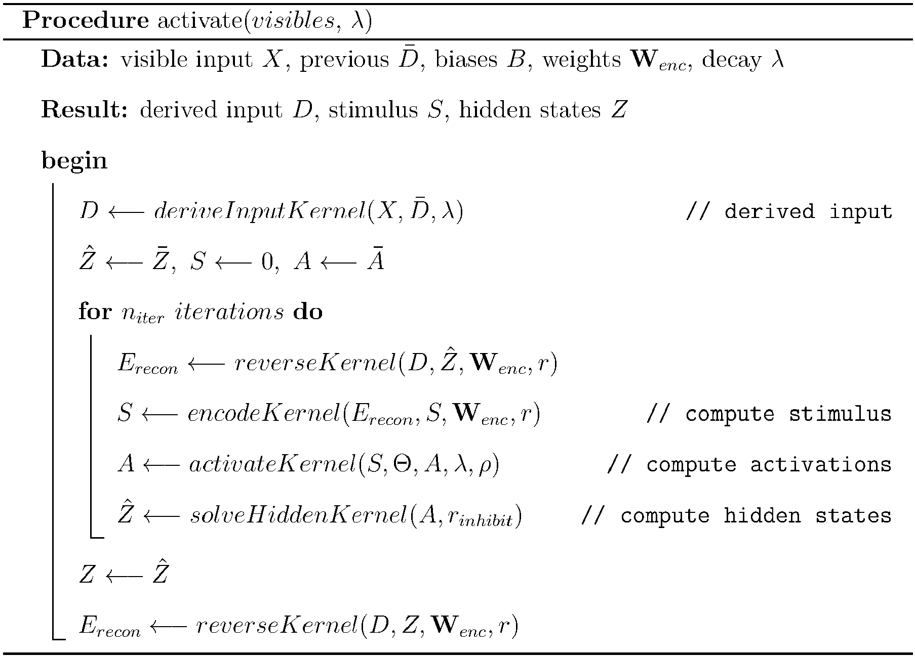 reverseKernel calculates the current reconstruction error given the current hidden solution and the derived inputs.
 encodeKernel produces the encoder's stimulus, which is a weighted sum of each unit's input reconstruction errors.
 activateKernel produces the encoder's activations from the stimulus.
 solveHiddenKernel implements local inhibition on the activations to produce a sparse binary hidden state.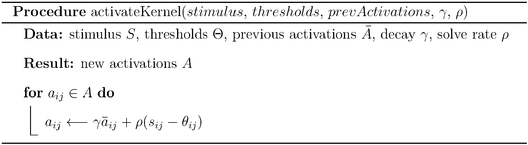
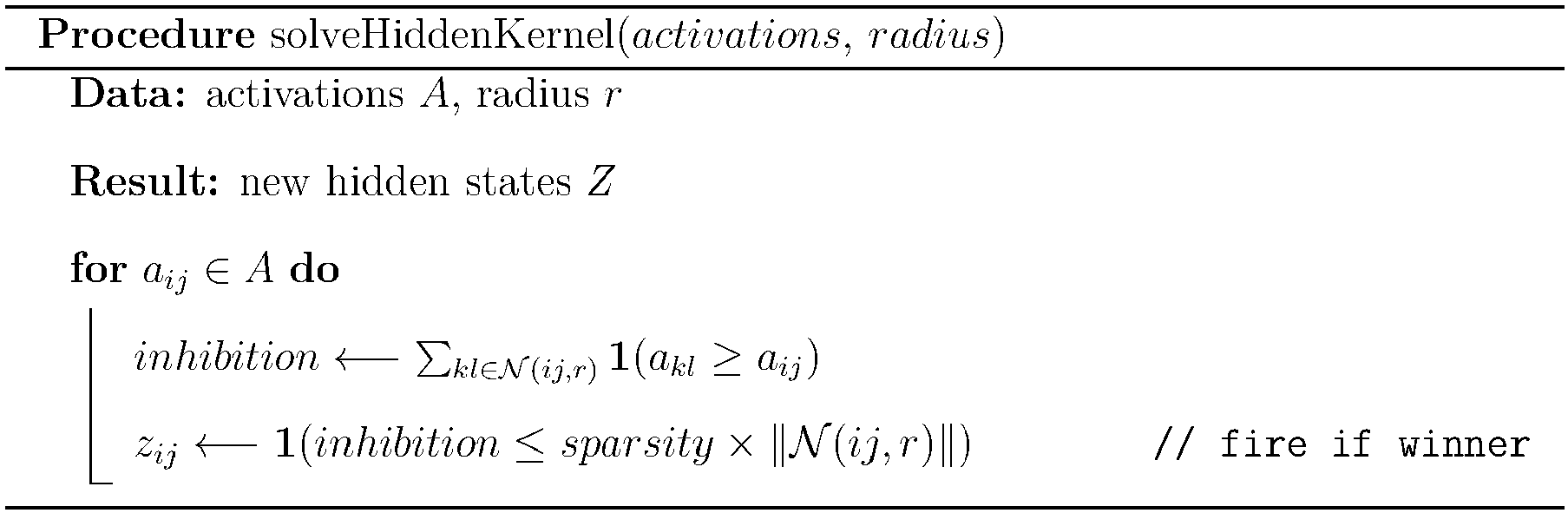
- The result of the iterative solving is a sparse code which represents a number of steps towards the minimisation of reconstruction errors of the encoder.
- Learning in the BISTA encoder is performed using a form of reconstruction error minimisation.

- In the following embodiment of the threshold update rule, we achieve lifetime sparsity in the state of a unit by incrementing the threshold when the state is too low (average below the target sparsity), and proportionally decrementing it when the state is too high (average above the target sparsity).

- Once the BISTA encoder has produced a sparse binary encoding of its input, the remainder of the hierarchy uses the SpikeProp encoders. encodeHierarchy() pass input into the hierarchy, and run the up-pass for each layer. First, the BISTA layer converts the inputs into a sparse binary hidden state, and then each successive layer builds its representation.

- The activateEncoder() and its kernels pass the hierarchy's inputs up from layer to layer. The encoding and decoding are combined.deriveInputKernel produces a pair of inputs to the encoder, one a copy of the input and the other a moving average of recent inputs.
 encodeKernel produces the encoder's stimulus, which is a weighted sum of each unit's derived inputs.
 activateKernel produces the encoder's activations from the stimulus, the previous activations, and the previous states. The activation is constrained non-negative by a Rectified Linear Unit.
 solveHiddenKernel implements local inhibition on the activations to produce a sparse binary hidden state.
 decodeKernel transforms the hidden inputs to the decoder using a weight matrix, forming a partial prediction.
 hierarchyLearn runs the learning for each layer's encoder.
 propagatelnputs reverses the decoding transformation to derive the stimulus for spike propagation.
 stimulusKernel computes the stimulus due to the raw inputs.
 learnEncoder uses a STDP-like mechanism to update the encoder weights, using the hidden state due to the input at each end of the weight's connection.
 learnDecoder updates lateral weights.

- In the following embodiment of the bias update rule, we achieve lifetime sparsity in the state of a unit by decrementing the bias when the stimulus is too high, and incrementing it when the stimulus is too low.

- When the computer begins the execution of the stored program code, each delay encoder is constructed in the memory of the system as follows (for m inputs and n outputs):
- 1. allocate 1-d arrays of length n for the activations, the previous activations, the output values, the previous outputs, the stimulus, the previous stimulus, the output traces, and the biases. Initialise to zero.
- 2. allocate 1-d arrays of length m for the inputs, the previous inputs, and the input traces. Initialise to zero.
- 3. allocate a 2-d n×m array of feedforward weights, output values, initially random and small, and a n × m array of feedforward traces, initially all zero.
- In the following, the symbol ⊙ refers to elementwise multiplication of same-sized vectors or matrices; ⊗ refers to an outer product of arbitrary vectors, forming a matrix result. J n is an n-dimensional vector of all 1's, and J n,m is an n × m-dimensional matrix of all I's. W i is the ith row of matrix W.
- Calculate the stimulus vector


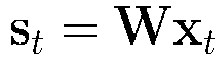


- Example code (in Python) for activation is as follows:


- Maintain a trace matrix T for previous activity taking reset into account (derived from Real-Time Recurrent Learning):

Determine importance of the feed forward weights:


- Example code (in Python) for learning is as follows:
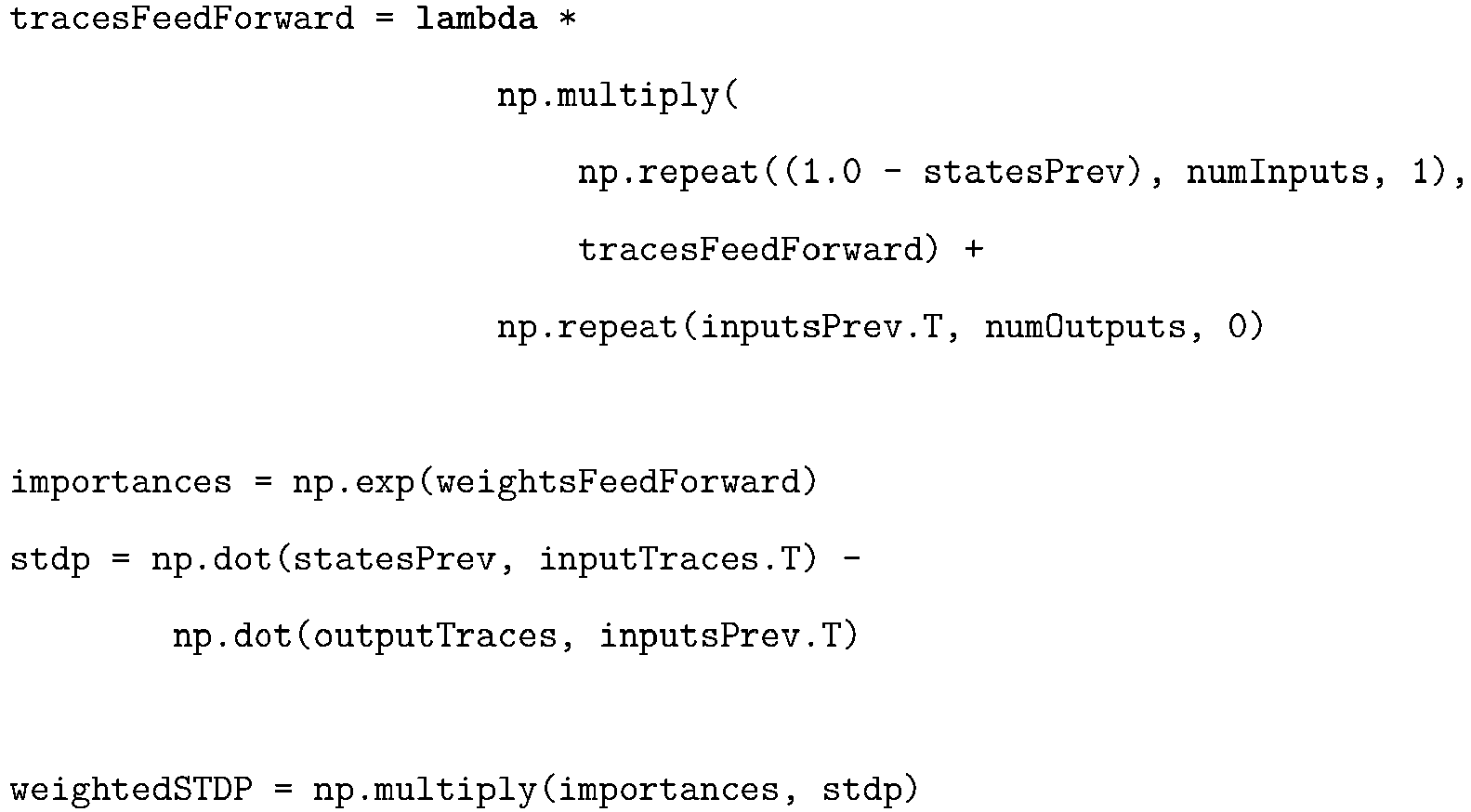

- The above learning rules represent a typical embodiment. Depending on the task, other embodiments may adapt these rules or use alternative rules. The Python code is provided only as an example, and a reader skilled in the art will understand that the system can be implemented in any modern computer language, depending on the platform and performance characteristics of relevance. For example, the system has been built and operated in C++ and Go as well as Python, and run on CPU and CPU/GPU systems.
- The Delay Encoder described elsewhere may be affected in terms of stability for certain embodiments or tasks as follows:
Calculate the importance-weighted spike time dependent plasticity (STDP) value for each connection: This change makes the STDP rule operate more symmetrically in time, so that the spiking pattern changes in the direction of the nearest correct output, whether this is backward or forward in time.
Further, the activation update can be modified to remove the non-linearity (max):
- The Chunk Encoder is an improved piece of componentry which may be used as a replacement for other encoders in the Predictive Hierarchy as described elsewhere in the instant application. The Chunk Encoder splits its output hidden state layer into small tiles called chunks, which operate as small, semi-independent self-organising representers of the underlying input data. Each chunk chooses a winning cell by inhibition for each timestep, and the weights in the chunk's units are updated to try to follow the winner for the given input.
- The primary procedures in the following which govern the operation of the hierarchy are activate and learn.
activate and its kernels pass the hierarchy's inputs up from layer to layer. The input is first combined with its historical values to generate a derived input, and then converted into a stimulus which is the size and shape of the output encoding. The stimulus is combined with each unit's bias to produce the activation (which may include information about previous stimuli), and finally the usually sparse hidden states are computed as the output of the encoder stage.
- The following listings contain example OpenCL kernel code for the Chunk Encoder.Listing 1: sfcDerivelnputs transforms the input into a delta of the input and previous trace, and a new trace value, a running average of previous inputs.
 Listing 2: sfcAddSample makes a shifted copy of the samples tensor samplesBack and adds the new input from visibleState at
index 0, placing the result in samplesFront.Listing 3: sfcStimulus computes the stimulus hiddenSummationTempFront by taking a window of inputs from visibleStates, subtracting a weight (taken from weights) from each input, and summing the squares. The result is normalised to the count of inputs, exponentiated and added to the previous stimulus. Listing 4: sfcActivate calculates the activations by adding the stimulus to the bias for each unit.
 Listing 5: sfcInhibit performs chunk-wise inhibition for each activation
 Listing 6: sfcInhibitOther performs chunk-wise inhibition on the encoder output states.
 Listing 7: sfcReconstruct forms a prediction from the encoder hidden states, using a linear transformation.
learn runs the learning kernel sfcLearnWeights in the Chunk Encoder. The learning mechanism operates on each chunk of hidden states, using the chunk winner as a target for each weight leading into a hidden unit. This target-following mechanism leads chunks of hidden units to behave as small self-organising maps (SOM's). The strength of the influence of the chunk winner on the hidden unit exponentially decays with the distance to the winner, and the weight is updated a little in the direction of the sampled input. The weight tensor W enc is indexed by i,j for the input plane, by k,l for the hidden unit plane, and by m for the nsample samples. Listing 8: sfcLearnWeights

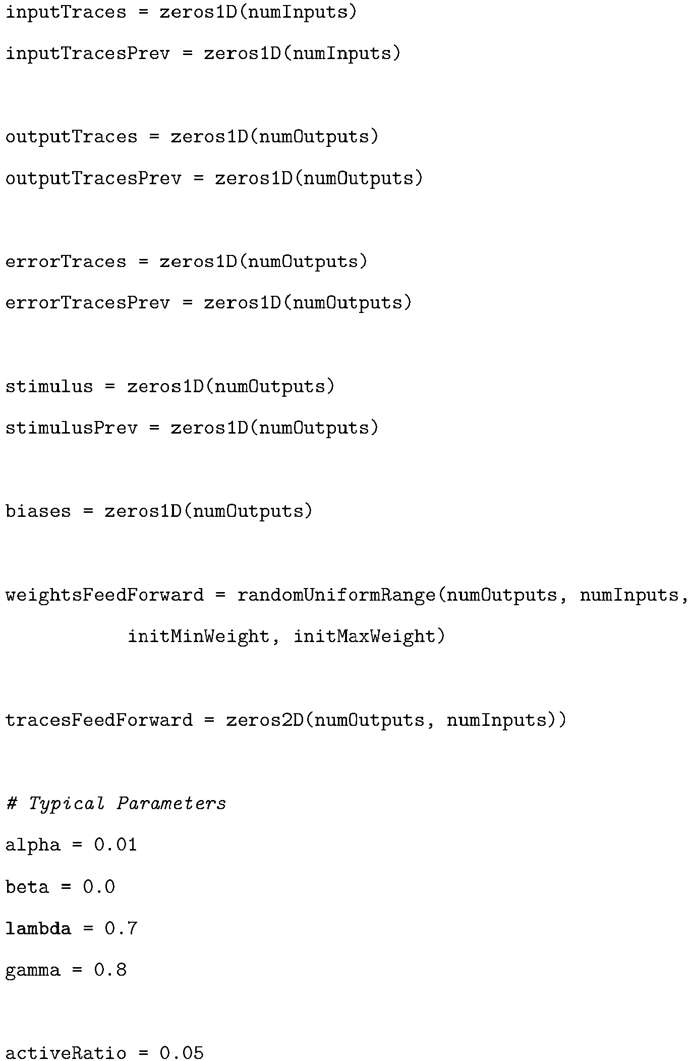
void kernel sfcLearnBiases(read_only image2d_t hiddenStimuli,
    read_only image2d_t hiddenStates, read_only image2d_t biasesBack,
    write_only image2d_t biasesFront, float activeRatio, float biasalpha)
    { int2 hiddenPosition = (int2)(get_global_id(0), get_global_id(1));
    float hiddenState = read_imagef(hiddenStates, defaultSampler, hiddenPosition).x;
    float hiddenStimulus = read_imagef(hiddenStimuli, defaultSampler, hiddenPosition).x;
    // Bias update
    float biasPrev = read_imagef(biasesBack, defaultSampler, hiddenPosition).x;
    write_imagef(biasesFront, hiddenPosition,
        (float4)(biasPrev + biasalpha * (activeRatio - hiddenState)));
        }
Listing 9: sfcLearnBiases


Claims (3)
- An apparatus (33) for detecting anomalous patterns in output of medical sensors monitoring a patient, the output of the medical sensors providing streams of time-varying data, the apparatus (33) comprising:processing means configured to implement first through N-th processing stages (53), N>1, each i-th processing stage (i = 1 to N) of the first through N-th processing stages (53) including an encoder (1) and a respective decoder (2),the encoder (1) of the first processing stage (53) having an input (3) configured to receive, as a sequence of input values, the streams of time-varying data, and an output configured to produce, as a sequence of encoded values, an encoded stream of time-varying data, each encoded value based upon both a current input value of the streams of time-varying data received by that encoder (1) and a set of previous input values of the streams of time-varying data received by that encoder (1), the input (3) of the encoder (1) of the first processing stage providing an input of the apparatus,the encoder (1) of each i-th processing stage (53), for i greater than 1, having an input (3) configured to receive, as a sequence of input values, a respective stream of time-varying data and an output (5) configured to produce, as a sequence of encoded values, a respective encoded stream of time- varying data, each encoded value based upon both a current input value of the stream of time-varying data received by that encoder (1) and a set of previous input values of the stream of time-varying data received by that encoder (1), the output of the encoder (1) of each i-th processing stage except the N-th processing stage coupled to the input (3) of the encoder (1) of the (i+1)-th processing stage,the decoder (2) of each i-th processing stage (53) having an input (3) coupled to the output of the respective encoder (1) of the same processing stage and an output configured to provide a prediction of an immediately next input value that will be received at the input (3) of the respective encoder (1) of the same processing stage, the output of the decoder (2) of each i-th processing stage (53) except the first processing stage (53) configured to provide the respective prediction as feedback to the decoder (2) of the (i-1)-th processing stage (53), the output of the decoder (2) of the first processing stage providing an output of the apparatus (33), characterized in thatthe first through N-th processing stages (53) of the apparatus (33) are configured to learn to model patterns of temporal evolution of the streams of time-varying data from the output of the medical sensors and to detect, based on the learned modeling of these patterns, an anomalous pattern in the output of the medical sensors that indicates a potential health risk to the patient,wherein each of the first through N-th processing stages (53) is coupled to a timing reference, the timing reference configured to produce a sequence of time steps,wherein the encoders (1) in the first through N-th processing stages (53) are configured to generate respective encoded values at their respective outputs in order from first through N-th during a current time step,wherein the decoders (2) in the first through N-th processing stages (53) are configured to generate respective predictions at their respective outputs in reverse order from N-th to first during the current time step, the prediction from the decoder (2) of the first processing stage (53) configured to predict an immediately next input value of the time-varying data that will be received at the input of the encoder (1) of the first processing stage (53) during an immediately next time step,wherein each of the decoders (2) in the first through N-th processing stages (53) is configured to generate the respective prediction during the current time step but after the respective encoder (11) has produced a respective encoded value of the encoded stream of time-varying data during the current time step,wherein the encoders of higher processing stages combine inputs over a small number of timesteps, ns , to produce more slowly varying encodings than do lower processing stages, in a striding process, wherein a corresponding destriding process is performed from higher to lower processing stages by the decoders, and wherein, at each processing stage, ns is the same for the encoder and the decoder and depends on the processing stages.
- The apparatus (33) of claim 1, wherein the apparatus (33) is configured to generate an output value at the output of the apparatus from an input value from the streams of time-varying data received at the input of the apparatus by way of a single processing path that starts at the encoder (1) of the first processing stage (53) and proceeds, in a single direction and without reversal, from the encoder (1) of the first processing stage (53), to the encoder (1) of the N-th processing stage (53), to the decoder (2) of the Nth processing stage (53), and to the decoder (2) of the first processing stage (53).
- The apparatus (33) of claim 2, wherein the apparatus (33) is configured to produce a new output value at the output of the apparatus, based on a new input value from the streams of time-varying data received at the input of the apparatus, during each of multiple successive time steps by processing each new input value received at the input of the apparatus (33) via the single processing path to generate the respective output value of the apparatus, each new output value produced at the output of the apparatus (33) during each time step providing a prediction of a new input value that will be received at the input of the apparatus (33) during a respective immediate next time step.
Applications Claiming Priority (5)
| Application Number | Priority Date | Filing Date | Title |
|---|---|---|---|
| US201662341790P | 2016-05-26 | 2016-05-26 | |
| US201662382992P | 2016-09-02 | 2016-09-02 | |
| US201662424226P | 2016-11-18 | 2016-11-18 | |
| US201762464090P | 2017-02-27 | 2017-02-27 | |
| PCT/US2017/034867 WO2017205850A1 (en) | 2016-05-26 | 2017-05-26 | Processing time-varying data streams using sparse predictive hierarchies |
Publications (2)
| Publication Number | Publication Date |
|---|---|
| EP3465551A1 EP3465551A1 (en) | 2019-04-10 |
| EP3465551B1 true EP3465551B1 (en) | 2024-05-15 |
Family
ID=59153275
Family Applications (1)
| Application Number | Title | Priority Date | Filing Date |
|---|---|---|---|
| EP17732643.6A Active EP3465551B1 (en) | 2016-05-26 | 2017-05-26 | Processing time-varying data streams using sparse predictive hierarchies |
Country Status (3)
| Country | Link |
|---|---|
| US (1) | US10579929B2 (en) |
| EP (1) | EP3465551B1 (en) |
| WO (1) | WO2017205850A1 (en) |
Families Citing this family (17)
| Publication number | Priority date | Publication date | Assignee | Title |
|---|---|---|---|---|
| US11875245B1 (en) * | 2018-02-22 | 2024-01-16 | United States Of America As Represented By The Secretary Of The Air Force | System, apparatus and method for spiking neural network |
| CN108814585B (en) * | 2018-05-03 | 2021-05-28 | 深圳竹信科技有限公司 | ECG signal processing method, device and computer-readable storage medium |
| CN109543727B (en) * | 2018-11-07 | 2022-12-20 | 复旦大学 | A semi-supervised anomaly detection method based on competitive reconstruction learning |
| US11689726B2 (en) * | 2018-12-05 | 2023-06-27 | Google Llc | Hybrid motion-compensated neural network with side-information based video coding |
| US11601644B2 (en) * | 2018-12-11 | 2023-03-07 | Google Llc | Image and video coding using machine learning prediction coding models |
| EP3722998A1 (en) * | 2019-04-11 | 2020-10-14 | Teraki GmbH | Data analytics on pre-processed signals |
| US20200401876A1 (en) * | 2019-06-24 | 2020-12-24 | Washington University | Method for designing scalable and energy-efficient analog neuromorphic processors |
| US11245600B2 (en) * | 2019-07-18 | 2022-02-08 | Citrix Systems, Inc. | System and method for processing network data |
| DE102019217073A1 (en) * | 2019-11-06 | 2021-05-06 | Robert Bosch Gmbh | Method for determining an impermissible deviation of the system behavior of a technical facility from a standard value range |
| CN112990053B (en) * | 2021-03-29 | 2023-07-25 | 腾讯科技(深圳)有限公司 | Image processing method, device, equipment and storage medium |
| US12266431B2 (en) * | 2021-04-05 | 2025-04-01 | Cerner Innovation, Inc. | Machine learning engine and rule engine for document auto-population using historical and contextual data |
| US12135529B2 (en) | 2021-12-14 | 2024-11-05 | Applied Materials, Inc. | Post preventative maintenance chamber condition monitoring and simulation |
| US20230222394A1 (en) * | 2022-01-07 | 2023-07-13 | Applied Materials, Inc. | Predictive modeling for chamber condition monitoring |
| TWI816579B (en) * | 2022-10-14 | 2023-09-21 | 財團法人工業技術研究院 | Network intrusion detecting system and network intrusion detecting method |
| US12530022B2 (en) | 2023-01-23 | 2026-01-20 | Applied Materials, Inc. | Process chamber qualification for maintenance process endpoint detection |
| CN117725543B (en) * | 2024-02-18 | 2024-05-03 | 中国民航大学 | Multi-element time sequence anomaly prediction method, electronic equipment and storage medium |
| CN118428547B (en) * | 2024-05-17 | 2024-12-13 | 南京邮电大学 | A link prediction method, system and storage medium for highly sparse mobile social networks |
Family Cites Families (1)
| Publication number | Priority date | Publication date | Assignee | Title |
|---|---|---|---|---|
| US11353833B2 (en) * | 2016-08-08 | 2022-06-07 | Goldman Sachs & Co. LLC | Systems and methods for learning and predicting time-series data using deep multiplicative networks |
-
2017
- 2017-05-26 US US16/304,396 patent/US10579929B2/en active Active
- 2017-05-26 EP EP17732643.6A patent/EP3465551B1/en active Active
- 2017-05-26 WO PCT/US2017/034867 patent/WO2017205850A1/en not_active Ceased
Also Published As
| Publication number | Publication date |
|---|---|
| US20190294980A1 (en) | 2019-09-26 |
| US10579929B2 (en) | 2020-03-03 |
| WO2017205850A1 (en) | 2017-11-30 |
| EP3465551A1 (en) | 2019-04-10 |
Similar Documents
| Publication | Publication Date | Title |
|---|---|---|
| US10579929B2 (en) | Processing time-varying data streams using sparse predictive hierarchies | |
| Millidge et al. | Predictive coding: a theoretical and experimental review | |
| Kriegeskorte et al. | Cognitive computational neuroscience | |
| Boerlin et al. | Predictive coding of dynamical variables in balanced spiking networks | |
| US20220383126A1 (en) | Low-Rank Adaptation of Neural Network Models | |
| Becker | Unsupervised learning procedures for neural networks | |
| US20190114391A1 (en) | Deep Learning-Based Aberrant Splicing Detection | |
| JP2021500654A (en) | Promoting the efficiency of neural networks | |
| Ororbia et al. | Backpropagation-free deep learning with recursive local representation alignment | |
| Ororbia et al. | Backprop-free reinforcement learning with active neural generative coding | |
| Bahmer et al. | Modern artificial neural networks: Is evolution cleverer? | |
| Wauthier et al. | Sleep: Model reduction in deep active inference | |
| Gilson et al. | Spectral analysis of input spike trains by spike-timing-dependent plasticity | |
| Sarmashghi et al. | Integrating statistical and machine learning approaches for neural classification | |
| Huo et al. | Research on SNN Learning Algorithms and Networks Based on Biological Plausibility | |
| Philipona et al. | Model of granular layer encoding in the cerebellum | |
| Woźniak et al. | Deep learning incorporating biologically-inspired neural dynamics | |
| Liu et al. | Artificial neural networks condensation: A strategy to facilitate adaption of machine learning in medical settings by reducing computational burden | |
| CN114872040B (en) | Musculoskeletal robot control method and device based on cerebellum prediction and correction | |
| Soo | Recurrent neural networks in cognitive and vision neuroscience | |
| Jain | Computing over in-vitro predictive coding neural cultures | |
| Dzemyda et al. | Combining Multidimensional Scaling with Artificial Neural Networks | |
| Tandale | Sustainable brain-inspired networks and deep-learning methods in structural mechanics | |
| US20260050838A1 (en) | One-shot, automated, multi-seasonal autoregressive tabular-forecaster | |
| US20230316081A1 (en) | Meta-Learning Bi-Directional Gradient-Free Artificial Neural Networks |
Legal Events
| Date | Code | Title | Description |
|---|---|---|---|
| STAA | Information on the status of an ep patent application or granted ep patent |
Free format text: STATUS: UNKNOWN |
|
| STAA | Information on the status of an ep patent application or granted ep patent |
Free format text: STATUS: THE INTERNATIONAL PUBLICATION HAS BEEN MADE |
|
| PUAI | Public reference made under article 153(3) epc to a published international application that has entered the european phase |
Free format text: ORIGINAL CODE: 0009012 |
|
| STAA | Information on the status of an ep patent application or granted ep patent |
Free format text: STATUS: REQUEST FOR EXAMINATION WAS MADE |
|
| 17P | Request for examination filed |
Effective date: 20181116 |
|
| AK | Designated contracting states |
Kind code of ref document: A1 Designated state(s): AL AT BE BG CH CY CZ DE DK EE ES FI FR GB GR HR HU IE IS IT LI LT LU LV MC MK MT NL NO PL PT RO RS SE SI SK SM TR |
|
| AX | Request for extension of the european patent |
Extension state: BA ME |
|
| DAV | Request for validation of the european patent (deleted) | ||
| DAX | Request for extension of the european patent (deleted) | ||
| STAA | Information on the status of an ep patent application or granted ep patent |
Free format text: STATUS: EXAMINATION IS IN PROGRESS |
|
| 17Q | First examination report despatched |
Effective date: 20210514 |
|
| REG | Reference to a national code |
Ref country code: DE Ref legal event code: R079 Free format text: PREVIOUS MAIN CLASS: G06N0003040000 Ipc: G06N0003045500 Ref country code: DE Ref legal event code: R079 Ref document number: 602017081913 Country of ref document: DE Free format text: PREVIOUS MAIN CLASS: G06N0003040000 Ipc: G06N0003045500 |
|
| GRAP | Despatch of communication of intention to grant a patent |
Free format text: ORIGINAL CODE: EPIDOSNIGR1 |
|
| STAA | Information on the status of an ep patent application or granted ep patent |
Free format text: STATUS: GRANT OF PATENT IS INTENDED |
|
| INTG | Intention to grant announced |
Effective date: 20231215 |
|
| RIC1 | Information provided on ipc code assigned before grant |
Ipc: G06N 3/092 20230101ALN20231204BHEP Ipc: G06N 3/09 20230101ALN20231204BHEP Ipc: G06N 3/088 20230101ALN20231204BHEP Ipc: G06N 3/065 20230101ALI20231204BHEP Ipc: G06N 3/049 20230101ALI20231204BHEP Ipc: G06N 3/0455 20230101AFI20231204BHEP |
|
| GRAS | Grant fee paid |
Free format text: ORIGINAL CODE: EPIDOSNIGR3 |
|
| GRAA | (expected) grant |
Free format text: ORIGINAL CODE: 0009210 |
|
| STAA | Information on the status of an ep patent application or granted ep patent |
Free format text: STATUS: THE PATENT HAS BEEN GRANTED |
|
| AK | Designated contracting states |
Kind code of ref document: B1 Designated state(s): AL AT BE BG CH CY CZ DE DK EE ES FI FR GB GR HR HU IE IS IT LI LT LU LV MC MK MT NL NO PL PT RO RS SE SI SK SM TR |
|
| REG | Reference to a national code |
Ref country code: CH Ref legal event code: EP Ref country code: GB Ref legal event code: FG4D |
|
| REG | Reference to a national code |
Ref country code: DE Ref legal event code: R096 Ref document number: 602017081913 Country of ref document: DE |
|
| REG | Reference to a national code |
Ref country code: IE Ref legal event code: FG4D |
|
| REG | Reference to a national code |
Ref country code: LT Ref legal event code: MG9D |
|
| REG | Reference to a national code |
Ref country code: NL Ref legal event code: MP Effective date: 20240515 |
|
| PG25 | Lapsed in a contracting state [announced via postgrant information from national office to epo] |
Ref country code: IS Free format text: LAPSE BECAUSE OF FAILURE TO SUBMIT A TRANSLATION OF THE DESCRIPTION OR TO PAY THE FEE WITHIN THE PRESCRIBED TIME-LIMIT Effective date: 20240915 |
|
| PG25 | Lapsed in a contracting state [announced via postgrant information from national office to epo] |
Ref country code: BG Free format text: LAPSE BECAUSE OF FAILURE TO SUBMIT A TRANSLATION OF THE DESCRIPTION OR TO PAY THE FEE WITHIN THE PRESCRIBED TIME-LIMIT Effective date: 20240515 |
|
| PG25 | Lapsed in a contracting state [announced via postgrant information from national office to epo] |
Ref country code: FI Free format text: LAPSE BECAUSE OF FAILURE TO SUBMIT A TRANSLATION OF THE DESCRIPTION OR TO PAY THE FEE WITHIN THE PRESCRIBED TIME-LIMIT Effective date: 20240515 Ref country code: HR Free format text: LAPSE BECAUSE OF FAILURE TO SUBMIT A TRANSLATION OF THE DESCRIPTION OR TO PAY THE FEE WITHIN THE PRESCRIBED TIME-LIMIT Effective date: 20240515 |
|
| PG25 | Lapsed in a contracting state [announced via postgrant information from national office to epo] |
Ref country code: GR Free format text: LAPSE BECAUSE OF FAILURE TO SUBMIT A TRANSLATION OF THE DESCRIPTION OR TO PAY THE FEE WITHIN THE PRESCRIBED TIME-LIMIT Effective date: 20240816 |
|
| PG25 | Lapsed in a contracting state [announced via postgrant information from national office to epo] |
Ref country code: PT Free format text: LAPSE BECAUSE OF FAILURE TO SUBMIT A TRANSLATION OF THE DESCRIPTION OR TO PAY THE FEE WITHIN THE PRESCRIBED TIME-LIMIT Effective date: 20240916 |
|
| REG | Reference to a national code |
Ref country code: AT Ref legal event code: MK05 Ref document number: 1687507 Country of ref document: AT Kind code of ref document: T Effective date: 20240515 |
|
| PG25 | Lapsed in a contracting state [announced via postgrant information from national office to epo] |
Ref country code: NL Free format text: LAPSE BECAUSE OF FAILURE TO SUBMIT A TRANSLATION OF THE DESCRIPTION OR TO PAY THE FEE WITHIN THE PRESCRIBED TIME-LIMIT Effective date: 20240515 |
|
| PG25 | Lapsed in a contracting state [announced via postgrant information from national office to epo] |
Ref country code: ES Free format text: LAPSE BECAUSE OF FAILURE TO SUBMIT A TRANSLATION OF THE DESCRIPTION OR TO PAY THE FEE WITHIN THE PRESCRIBED TIME-LIMIT Effective date: 20240515 |
|
| PG25 | Lapsed in a contracting state [announced via postgrant information from national office to epo] |
Ref country code: AT Free format text: LAPSE BECAUSE OF FAILURE TO SUBMIT A TRANSLATION OF THE DESCRIPTION OR TO PAY THE FEE WITHIN THE PRESCRIBED TIME-LIMIT Effective date: 20240515 |
|
| PG25 | Lapsed in a contracting state [announced via postgrant information from national office to epo] |
Ref country code: PL Free format text: LAPSE BECAUSE OF FAILURE TO SUBMIT A TRANSLATION OF THE DESCRIPTION OR TO PAY THE FEE WITHIN THE PRESCRIBED TIME-LIMIT Effective date: 20240515 |
|
| PG25 | Lapsed in a contracting state [announced via postgrant information from national office to epo] |
Ref country code: LV Free format text: LAPSE BECAUSE OF FAILURE TO SUBMIT A TRANSLATION OF THE DESCRIPTION OR TO PAY THE FEE WITHIN THE PRESCRIBED TIME-LIMIT Effective date: 20240515 |
|
| PG25 | Lapsed in a contracting state [announced via postgrant information from national office to epo] |
Ref country code: PT Free format text: LAPSE BECAUSE OF FAILURE TO SUBMIT A TRANSLATION OF THE DESCRIPTION OR TO PAY THE FEE WITHIN THE PRESCRIBED TIME-LIMIT Effective date: 20240916 Ref country code: PL Free format text: LAPSE BECAUSE OF FAILURE TO SUBMIT A TRANSLATION OF THE DESCRIPTION OR TO PAY THE FEE WITHIN THE PRESCRIBED TIME-LIMIT Effective date: 20240515 Ref country code: NO Free format text: LAPSE BECAUSE OF FAILURE TO SUBMIT A TRANSLATION OF THE DESCRIPTION OR TO PAY THE FEE WITHIN THE PRESCRIBED TIME-LIMIT Effective date: 20240815 Ref country code: NL Free format text: LAPSE BECAUSE OF FAILURE TO SUBMIT A TRANSLATION OF THE DESCRIPTION OR TO PAY THE FEE WITHIN THE PRESCRIBED TIME-LIMIT Effective date: 20240515 Ref country code: LV Free format text: LAPSE BECAUSE OF FAILURE TO SUBMIT A TRANSLATION OF THE DESCRIPTION OR TO PAY THE FEE WITHIN THE PRESCRIBED TIME-LIMIT Effective date: 20240515 Ref country code: IS Free format text: LAPSE BECAUSE OF FAILURE TO SUBMIT A TRANSLATION OF THE DESCRIPTION OR TO PAY THE FEE WITHIN THE PRESCRIBED TIME-LIMIT Effective date: 20240915 Ref country code: HR Free format text: LAPSE BECAUSE OF FAILURE TO SUBMIT A TRANSLATION OF THE DESCRIPTION OR TO PAY THE FEE WITHIN THE PRESCRIBED TIME-LIMIT Effective date: 20240515 Ref country code: GR Free format text: LAPSE BECAUSE OF FAILURE TO SUBMIT A TRANSLATION OF THE DESCRIPTION OR TO PAY THE FEE WITHIN THE PRESCRIBED TIME-LIMIT Effective date: 20240816 Ref country code: FI Free format text: LAPSE BECAUSE OF FAILURE TO SUBMIT A TRANSLATION OF THE DESCRIPTION OR TO PAY THE FEE WITHIN THE PRESCRIBED TIME-LIMIT Effective date: 20240515 Ref country code: ES Free format text: LAPSE BECAUSE OF FAILURE TO SUBMIT A TRANSLATION OF THE DESCRIPTION OR TO PAY THE FEE WITHIN THE PRESCRIBED TIME-LIMIT Effective date: 20240515 Ref country code: BG Free format text: LAPSE BECAUSE OF FAILURE TO SUBMIT A TRANSLATION OF THE DESCRIPTION OR TO PAY THE FEE WITHIN THE PRESCRIBED TIME-LIMIT Effective date: 20240515 Ref country code: AT Free format text: LAPSE BECAUSE OF FAILURE TO SUBMIT A TRANSLATION OF THE DESCRIPTION OR TO PAY THE FEE WITHIN THE PRESCRIBED TIME-LIMIT Effective date: 20240515 Ref country code: RS Free format text: LAPSE BECAUSE OF FAILURE TO SUBMIT A TRANSLATION OF THE DESCRIPTION OR TO PAY THE FEE WITHIN THE PRESCRIBED TIME-LIMIT Effective date: 20240815 |
|
| REG | Reference to a national code |
Ref country code: CH Ref legal event code: PL |
|
| PG25 | Lapsed in a contracting state [announced via postgrant information from national office to epo] |
Ref country code: DK Free format text: LAPSE BECAUSE OF FAILURE TO SUBMIT A TRANSLATION OF THE DESCRIPTION OR TO PAY THE FEE WITHIN THE PRESCRIBED TIME-LIMIT Effective date: 20240515 |
|
| PG25 | Lapsed in a contracting state [announced via postgrant information from national office to epo] |
Ref country code: LU Free format text: LAPSE BECAUSE OF NON-PAYMENT OF DUE FEES Effective date: 20240526 |
|
| PG25 | Lapsed in a contracting state [announced via postgrant information from national office to epo] |
Ref country code: EE Free format text: LAPSE BECAUSE OF FAILURE TO SUBMIT A TRANSLATION OF THE DESCRIPTION OR TO PAY THE FEE WITHIN THE PRESCRIBED TIME-LIMIT Effective date: 20240515 |
|
| PG25 | Lapsed in a contracting state [announced via postgrant information from national office to epo] |
Ref country code: CZ Free format text: LAPSE BECAUSE OF FAILURE TO SUBMIT A TRANSLATION OF THE DESCRIPTION OR TO PAY THE FEE WITHIN THE PRESCRIBED TIME-LIMIT Effective date: 20240515 |
|
| PG25 | Lapsed in a contracting state [announced via postgrant information from national office to epo] |
Ref country code: SK Free format text: LAPSE BECAUSE OF FAILURE TO SUBMIT A TRANSLATION OF THE DESCRIPTION OR TO PAY THE FEE WITHIN THE PRESCRIBED TIME-LIMIT Effective date: 20240515 Ref country code: RO Free format text: LAPSE BECAUSE OF FAILURE TO SUBMIT A TRANSLATION OF THE DESCRIPTION OR TO PAY THE FEE WITHIN THE PRESCRIBED TIME-LIMIT Effective date: 20240515 |
|
| PG25 | Lapsed in a contracting state [announced via postgrant information from national office to epo] |
Ref country code: SM Free format text: LAPSE BECAUSE OF FAILURE TO SUBMIT A TRANSLATION OF THE DESCRIPTION OR TO PAY THE FEE WITHIN THE PRESCRIBED TIME-LIMIT Effective date: 20240515 |
|
| PG25 | Lapsed in a contracting state [announced via postgrant information from national office to epo] |
Ref country code: SM Free format text: LAPSE BECAUSE OF FAILURE TO SUBMIT A TRANSLATION OF THE DESCRIPTION OR TO PAY THE FEE WITHIN THE PRESCRIBED TIME-LIMIT Effective date: 20240515 Ref country code: SK Free format text: LAPSE BECAUSE OF FAILURE TO SUBMIT A TRANSLATION OF THE DESCRIPTION OR TO PAY THE FEE WITHIN THE PRESCRIBED TIME-LIMIT Effective date: 20240515 Ref country code: RO Free format text: LAPSE BECAUSE OF FAILURE TO SUBMIT A TRANSLATION OF THE DESCRIPTION OR TO PAY THE FEE WITHIN THE PRESCRIBED TIME-LIMIT Effective date: 20240515 Ref country code: LU Free format text: LAPSE BECAUSE OF NON-PAYMENT OF DUE FEES Effective date: 20240526 Ref country code: EE Free format text: LAPSE BECAUSE OF FAILURE TO SUBMIT A TRANSLATION OF THE DESCRIPTION OR TO PAY THE FEE WITHIN THE PRESCRIBED TIME-LIMIT Effective date: 20240515 Ref country code: DK Free format text: LAPSE BECAUSE OF FAILURE TO SUBMIT A TRANSLATION OF THE DESCRIPTION OR TO PAY THE FEE WITHIN THE PRESCRIBED TIME-LIMIT Effective date: 20240515 Ref country code: CZ Free format text: LAPSE BECAUSE OF FAILURE TO SUBMIT A TRANSLATION OF THE DESCRIPTION OR TO PAY THE FEE WITHIN THE PRESCRIBED TIME-LIMIT Effective date: 20240515 Ref country code: CH Free format text: LAPSE BECAUSE OF NON-PAYMENT OF DUE FEES Effective date: 20240531 |
|
| PG25 | Lapsed in a contracting state [announced via postgrant information from national office to epo] |
Ref country code: IT Free format text: LAPSE BECAUSE OF FAILURE TO SUBMIT A TRANSLATION OF THE DESCRIPTION OR TO PAY THE FEE WITHIN THE PRESCRIBED TIME-LIMIT Effective date: 20240515 Ref country code: MC Free format text: LAPSE BECAUSE OF FAILURE TO SUBMIT A TRANSLATION OF THE DESCRIPTION OR TO PAY THE FEE WITHIN THE PRESCRIBED TIME-LIMIT Effective date: 20240515 |
|
| REG | Reference to a national code |
Ref country code: DE Ref legal event code: R097 Ref document number: 602017081913 Country of ref document: DE |
|
| REG | Reference to a national code |
Ref country code: BE Ref legal event code: MM Effective date: 20240531 |
|
| PLBE | No opposition filed within time limit |
Free format text: ORIGINAL CODE: 0009261 |
|
| STAA | Information on the status of an ep patent application or granted ep patent |
Free format text: STATUS: NO OPPOSITION FILED WITHIN TIME LIMIT |
|
| PG25 | Lapsed in a contracting state [announced via postgrant information from national office to epo] |
Ref country code: IE Free format text: LAPSE BECAUSE OF NON-PAYMENT OF DUE FEES Effective date: 20240526 |
|
| 26N | No opposition filed |
Effective date: 20250218 |
|
| PG25 | Lapsed in a contracting state [announced via postgrant information from national office to epo] |
Ref country code: BE Free format text: LAPSE BECAUSE OF NON-PAYMENT OF DUE FEES Effective date: 20240531 Ref country code: SI Free format text: LAPSE BECAUSE OF FAILURE TO SUBMIT A TRANSLATION OF THE DESCRIPTION OR TO PAY THE FEE WITHIN THE PRESCRIBED TIME-LIMIT Effective date: 20240515 |
|
| PGFP | Annual fee paid to national office [announced via postgrant information from national office to epo] |
Ref country code: DE Payment date: 20250529 Year of fee payment: 9 |
|
| PGFP | Annual fee paid to national office [announced via postgrant information from national office to epo] |
Ref country code: GB Payment date: 20250527 Year of fee payment: 9 |
|
| PGFP | Annual fee paid to national office [announced via postgrant information from national office to epo] |
Ref country code: FR Payment date: 20250526 Year of fee payment: 9 |
|
| PG25 | Lapsed in a contracting state [announced via postgrant information from national office to epo] |
Ref country code: HU Free format text: LAPSE BECAUSE OF FAILURE TO SUBMIT A TRANSLATION OF THE DESCRIPTION OR TO PAY THE FEE WITHIN THE PRESCRIBED TIME-LIMIT; INVALID AB INITIO Effective date: 20170526 |
|
| PG25 | Lapsed in a contracting state [announced via postgrant information from national office to epo] |
Ref country code: SE Free format text: LAPSE BECAUSE OF FAILURE TO SUBMIT A TRANSLATION OF THE DESCRIPTION OR TO PAY THE FEE WITHIN THE PRESCRIBED TIME-LIMIT Effective date: 20240515 |
|
| PG25 | Lapsed in a contracting state [announced via postgrant information from national office to epo] |
Ref country code: CY Free format text: LAPSE BECAUSE OF FAILURE TO SUBMIT A TRANSLATION OF THE DESCRIPTION OR TO PAY THE FEE WITHIN THE PRESCRIBED TIME-LIMIT; INVALID AB INITIO Effective date: 20170526 |