EP3330812A1 - Method for controlling a technical system with a two degree of freedom controller and its parameterization - Google Patents
Method for controlling a technical system with a two degree of freedom controller and its parameterization Download PDFInfo
- Publication number
- EP3330812A1 EP3330812A1 EP16201898.0A EP16201898A EP3330812A1 EP 3330812 A1 EP3330812 A1 EP 3330812A1 EP 16201898 A EP16201898 A EP 16201898A EP 3330812 A1 EP3330812 A1 EP 3330812A1
- Authority
- EP
- European Patent Office
- Prior art keywords
- plant
- controller
- variable
- output
- nonlinear
- Prior art date
- Legal status (The legal status is an assumption and is not a legal conclusion. Google has not performed a legal analysis and makes no representation as to the accuracy of the status listed.)
- Granted
Links
Images





Classifications
-
- G—PHYSICS
- G05—CONTROLLING; REGULATING
- G05B—CONTROL OR REGULATING SYSTEMS IN GENERAL; FUNCTIONAL ELEMENTS OF SUCH SYSTEMS; MONITORING OR TESTING ARRANGEMENTS FOR SUCH SYSTEMS OR ELEMENTS
- G05B11/00—Automatic controllers
-
- G—PHYSICS
- G05—CONTROLLING; REGULATING
- G05B—CONTROL OR REGULATING SYSTEMS IN GENERAL; FUNCTIONAL ELEMENTS OF SUCH SYSTEMS; MONITORING OR TESTING ARRANGEMENTS FOR SUCH SYSTEMS OR ELEMENTS
- G05B13/00—Adaptive control systems, i.e. systems automatically adjusting themselves to have a performance which is optimum according to some preassigned criterion
- G05B13/02—Adaptive control systems, i.e. systems automatically adjusting themselves to have a performance which is optimum according to some preassigned criterion electric
- G05B13/04—Adaptive control systems, i.e. systems automatically adjusting themselves to have a performance which is optimum according to some preassigned criterion electric involving the use of models or simulators
-
- G—PHYSICS
- G05—CONTROLLING; REGULATING
- G05B—CONTROL OR REGULATING SYSTEMS IN GENERAL; FUNCTIONAL ELEMENTS OF SUCH SYSTEMS; MONITORING OR TESTING ARRANGEMENTS FOR SUCH SYSTEMS OR ELEMENTS
- G05B2219/00—Program-control systems
- G05B2219/20—Pc systems
- G05B2219/25—Pc structure of the system
- G05B2219/25409—Feedforward of control signal to compensate for delay in execution
-
- G—PHYSICS
- G05—CONTROLLING; REGULATING
- G05B—CONTROL OR REGULATING SYSTEMS IN GENERAL; FUNCTIONAL ELEMENTS OF SUCH SYSTEMS; MONITORING OR TESTING ARRANGEMENTS FOR SUCH SYSTEMS OR ELEMENTS
- G05B2219/00—Program-control systems
- G05B2219/30—Nc systems
- G05B2219/39—Robotics, robotics to robotics hand
- G05B2219/39301—Learn feedforward control
-
- G—PHYSICS
- G05—CONTROLLING; REGULATING
- G05B—CONTROL OR REGULATING SYSTEMS IN GENERAL; FUNCTIONAL ELEMENTS OF SUCH SYSTEMS; MONITORING OR TESTING ARRANGEMENTS FOR SUCH SYSTEMS OR ELEMENTS
- G05B2219/00—Program-control systems
- G05B2219/30—Nc systems
- G05B2219/41—Servomotor, servo controller till figures
- G05B2219/41012—Adjust feedforward gain
-
- G—PHYSICS
- G05—CONTROLLING; REGULATING
- G05B—CONTROL OR REGULATING SYSTEMS IN GENERAL; FUNCTIONAL ELEMENTS OF SUCH SYSTEMS; MONITORING OR TESTING ARRANGEMENTS FOR SUCH SYSTEMS OR ELEMENTS
- G05B2219/00—Program-control systems
- G05B2219/30—Nc systems
- G05B2219/41—Servomotor, servo controller till figures
- G05B2219/41233—Feedforward simulation filter, with model
-
- G—PHYSICS
- G05—CONTROLLING; REGULATING
- G05B—CONTROL OR REGULATING SYSTEMS IN GENERAL; FUNCTIONAL ELEMENTS OF SUCH SYSTEMS; MONITORING OR TESTING ARRANGEMENTS FOR SUCH SYSTEMS OR ELEMENTS
- G05B2219/00—Program-control systems
- G05B2219/30—Nc systems
- G05B2219/41—Servomotor, servo controller till figures
- G05B2219/41453—Inverse, feedforward controller is inverse of closed loop system
-
- G—PHYSICS
- G05—CONTROLLING; REGULATING
- G05B—CONTROL OR REGULATING SYSTEMS IN GENERAL; FUNCTIONAL ELEMENTS OF SUCH SYSTEMS; MONITORING OR TESTING ARRANGEMENTS FOR SUCH SYSTEMS OR ELEMENTS
- G05B2219/00—Program-control systems
- G05B2219/30—Nc systems
- G05B2219/42—Servomotor, servo controller kind till VSS
- G05B2219/42065—Feedforward combined with pid feedback
Definitions
- the invention pertains to a method for controlling a technical system as plant with a Two Degree of Freedom controller having a feedforward controller providing an output and a feedback controller providing an output whereas the feedforward controller uses an inverse of the plant and the Two Degree of Freedom controller is designed to calculate a control variable of the plant from the output of the feedforward controller and the output of the feedback controller to achieve a setpoint value of an output variable of the plant in dependence from a state variable of the plant. Furthermore, the invention pertains to the parameterization of the Two Degree of Freedom controller for controlling the technical system.
- a plant also often called controlled system
- a plant represents the technical system to be controlled.
- An example of a technical system is an engine testbed on which the engine torque of the internal combustion engine (unit under test on the testbed) has to be controlled in accordance to set reference values (e.g. a demanded torque).
- the controller has to be designed and/or parameterized to adapt the controller to the static and dynamic behaviour of the actual plant. Only a correctly tuned controller is able to adequately and sufficiently control the plant, e.g. with respect to control error, stability, controllability, etc. Many plants, however, show a (highly) nonlinear dynamic behaviour in practice, which makes the controller design and/or parameterization difficult.
- a given controller design with a set of controller parameters is used for a given plant or control task which is then only parameterized (assigning values to the controller parameters) by tuning the controller parameters in order to achieve a desired, given control behaviour.
- the controller design can be simple, tuning of the controller parameters has proven to be difficult because of the nonlinear behaviour of the plant. Therefore often highly trained and experienced experts are required to successfully parameterize such a controller.
- an Enhanced Progressive Adaptive Controller is often used for the engine testbed example, but also for other testbed applications as e.g. for a transmission testbed, drive train testbed, vehicle testbed, roller testbed, etc.
- an Enhanced Progressive Adaptive Controller is often used.
- tuning of an ENPAC is a rather difficult and time consuming task.
- controllers There are of course also other controller designs known. Especially a known Two Degree of Freedom (2DoF) controller is well suited for many applications, as such controller show good reference tracking performance and disturbance rejection.
- 2DoF Two Degree of Freedom
- the problem with such a controller is that the controller uses an inversion of the plant in the feedforward part of the controller. For a linear plant, an inversion is usually easy to determine. But this does not apply to a nonlinear plant. Therefore a 2DoF controller cannot easily be used for controlling a nonlinear plant.
- a Two Degree of Freedom controller for designing and parameterizing such a Two Degree of Freedom (2DoF) controller for a nonlinear plant, which preferably allows also an automated parameterization of the controller.
- the inverse of the plant is constituted by a nonlinear dynamic part and a nonlinear static part
- a static map of the plant is provided that maps the control variable and the state variable onto the output variable and the nonlinear static part is formed by an inverse of this static map
- the plant is modelled with a model with a chosen model structure having system parameters and that the nonlinear dynamic part is formed as function of the system parameters of the model and of a desired output variable of a desired closed loop behaviour of the plant and the output of the nonlinear dynamic part and the state variable are fed into the inverse of the static map of the nonlinear static part that outputs the control variable for controlling the plant.
- nonlinear static and nonlinear dynamic part it is possible to approximate the inverse of the nonlinear plant model, which can then be used in the feedforward controller.
- the nonlinear dynamic part approximates the dynamic behaviour of the plant and the nonlinear static part the static behaviour.
- By modelling the nonlinear static part as static map it is possible to determine its inverse which is fed by the output of the nonlinear dynamic part.
- This controller can be parameterized by carrying out a first defined testrun on the testbed with the unit under test and by collecting first testrun data during the first testrun which is used to identify the static map of the plant that maps the control variable and the state variable onto the output variable and this static map is inverted to form the nonlinear static part of the feedforward controller, and by carrying out a second defined testrun on the testbed with the unit under test and by collecting second testrun data during the second testrun which is used for identification of the system parameters of the model of the plant for the nonlinear dynamic part.
- This allows for an easy parameterization of the Two Degree of Freedom controller, or its feedforward controller, with an easy to follow routine that could also be performed fully automatically on the test bed.
- the feedback controller can be regarded as being parameterized, as its parameters are easy to parameterize or to tune, especially as there are no high demands on the feedback controller.
- Fig.1 the general and well known controller structure of a Two Degree of Freedom (2DoF) controller 2 for controlling a plant 1 is shown.
- the Two Degree of Freedom controller 2 comprises a feedforward controller 3 and a feedback controller 4.
- a Two Degree of Freedom (2DoF) controller 2 with two degrees of freedom can be used as is shown in Fig.1 .
- the plant 1 is a dynamic technical system that needs to be controlled.
- the technical system is for example a testbed 10 with a unit under test 11 arranged and operated on the testbed 10 as shown in Fig.2 .
- the load machine 13 can also be part of the plant 1.
- the testbed 10 can be an engine testbed with an internal combustion engine 14 as unit under test 11 that is connected to a dynamometer (e.g. an electric motor or a water brake dynamometer) as load machine 13.
- a dynamometer e.g. an electric motor or a water brake dynamometer
- the plant 1 is controlled with a control variable u calculated by the controller 2 which is implemented (software and/or hardware) in a plant control unit 15.
- the control variable u is e.g. used to adjust at least one actuator of the plant 1.
- the control variable u of an engine 14 can be the percentage ⁇ of the applied throttle pedal, for example.
- the controller 2 controls an output variable y of the plant 1 according to a given setpoint y set .
- the setpoint y set can be a demanded torque T D , for example.
- the output variable y of an engine 14 is for example the actual engine torque T.
- the current value of the output variable y can be measured by a suitable sensor 16, e.g. a torque sensor, can be calculated by using a simulation model, e.g. of the unit under test 11, of a vehicle into which the unit under test 11 is arranged, etc., or can be estimated with an observer from other known (e.g. by measured) variables of the plant 1.
- the output variable y is fed back in known manner to the controller 2 for feedback control.
- the 2DoF controller 2 utilizes usually also certain state variables x of the plant 1, e.g. an engine speed n in case of an engine 14.
- the state variable x can be measured by using a sensor 17, can be calculated by using a simulation model, e.g. of the unit under test 11, of a vehicle into which the unit under test 11 is arranged, etc., or can be estimated with an observer for the state variable x from other known (e.g. measured) variables of the plant 1.
- the control variable u for the plant 1 calculated in the 2DoF controller 2 comprises a control variable u FF of the feedforward controller 3 and a control variable u FB of the feedback controller 4, which are summed to form the control variable u for the plant 1.
- the setpoint y set is fed to the feedforward controller 3 and to the feedback controller 4.
- the controller design is usually done with a (mathematical) model of the plant 1 that comprises also certain state variables x.
- the model of the plant 1 maps the input (control variable u) to the output y.
- the feedforward controller 3 embodies an inverse of the controlled plant 1, i.e. an inverse of the model of the plant 1.
- the model of a dynamic technical system as the plant 1 is usually nonlinear.
- the most challenging task of the design of the inventive 2DoF controller 2 is the implementation of the feedforward controller 3.
- the necessary inversion of the plant 1 according to the invention is described in the following, without limitation, on the example of a plant model having a known first order model structure.
- K is the gain and ⁇ the time constant, which are both given system parameters defined by the implementation of the plant 1 and can be regarded as being known.
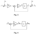
- the known model structure of the first order plant is shown in Fig.3 , where s represents the known Laplace operator.
- the parameters K and ⁇ , and also C1, C2 if present, are dependent from a current operating point (output variable y and state variable x at a certain point in time) of the dynamic system and the equation is nonlinear and therefore not directly invertible.
- a desired closed loop behaviour of the plant 1 is chosen as shown in Fig.4 .
- the chosen desired behaviour is defined by the desired time constant ⁇ des which produces a desired output variable y des .
- the structure of the desired plant ( Fig.4 ) is preferably the same as the structure of the plant model ( Fig.3 ). I.e., if the response of the plant 1 can be characterized as a first order response, then the desired behaviour is preferably also a first order model, if the plant response is of second order then the desired behaviour is preferably of second order, and so on.
- the above equation comprises a nonlinear dynamic part ⁇ K y ⁇ des + 1 K y des and a nonlinear static part C 1 ⁇ 1 K C 2.
- the nonlinear dynamic part is a function of system parameters of the model of the plant 1 and of a desired output variable y des .
- a map 20 is exemplarily shown in Fig.5 for the example of an engine map for an engine 14, with the engine torque T as output variable y, the percentage ⁇ of the applied throttle pedal as control variable u and the engine speed n as state variable x.
- the function f is monotonically increasing over the entire range of the control variable u for a given state variable x, then it is easily possible to determine its inverse, i.e. the function f -1 , with known methods. For example the inverse could be found with help of the Matlab (Matlab is a known software of the company The MathWorks) function interp1(), that realises a 1-D data interpolation. This leads to the inverted map 21 of the map 20.
- Matlab Matlab is a known software of the company The MathWorks
- a monotonization step is carried out first.
- the monotonization can be done as described in the following with reference to Fig.6 .
- a map 20 is usually stored as multidimensional (according to the dimension of the map 20) table with multiple datapoints DP where every datapoint DP has the dimension of the map 20. Then the state variable x is held constant and the function of the output variable y in dependence from the control variable u is analysed. If the output variable y is not monotonically increasing over the entire range of the control variable u, the last datapoint D1 where the function is still monotonically increasing is searched. From this datapoint D1 and the datapoint D2 of the maximum value of the output variable y the slope of a line connecting the datapoints D1 and D2 is calculated. This slope is then added to all the datapoints DP in the region where the output variable y is not monotonically increasing.
- Fig.6 the dotted line shows the original non-monotonically increasing output variable function f and the solid line shows the resulting monotonized output variable function f. This is repeated for different values of the state variable x in order to obtain the monotonized map 20'.
- a known smoothing of the monotonized map 20' can be applied to all the manipulated datapoints DP. In this way a monotonically increasing output variable function f can be guaranteed and the shape of the original function f can basically be preserved.
- the map 20 is at least monotonically increasing along the axis of the control variable u (i.e. for a given, fixed state variable x).
- the resulting monotonized map 20' can then be inverted with known means as described above.
- the final inverted map 21 of the monotonized map 20' of the map 20 in Fig.5 is shown exemplarily in Fig.7 .
- the inverted map 21 outputs the control variable u (e.g. pedal position ⁇ ) for a given operating point, given by a state variable x (e.g. speed n) and a given output variable y (e.g. torque T).
- the above nonlinear static part C 1 ⁇ 1 K C 2 is embedded in the map 20 and consequently also in the inverted map 21.
- the nonlinear dynamic part ⁇ K y ⁇ des + 1 K y des comprises the system parameters ⁇ and K of the plant 1 as functions of the operating point of the system given by the output variable y and state variable x.
- the operating point could be given by the engine torque T and engine speed n.
- K the dynamic system is first identified and modelled with a local model network (LMN) that models the nonlinear dynamic behaviour of the system, i.e. the plant 1.
- the weighing is done with a validity function ⁇ i , which is a function of a scheduling vector ⁇ that defines the operating point of the system.
- the validity functions ⁇ i define the activation level of local models M i at a particular operating point (given as scheduling vector ⁇ ). This means that not every local model M i contributes in every operating point in the same amount to the estimation of the output variable ⁇ .
- a suitable model structure is chosen, usually a linear function of the data vector ⁇ and with local model parameters in form of a parameter vector ⁇ , although it is also possible to choose a nonlinear function as local Model M i .
- the estimation ⁇ of the output variable y could also be calculated from the LMN by blending the parameters ⁇ instead of blending the local outputs ⁇ i .
- the identified parameters a in , b im in the discrete time domain could be transformed into the continuous time domain, for example with the help of the well-known bilinear transformation.
- the system parameters K and ⁇ could also directly be identified using the chosen model structure, as e.g. shown in Fig.3 .
- a step could be applied as input u to the plant 1 and the output y could be recorded. Then the same input is applied to the chosen model structure and the parameters of the model, here e.g.
- parameters K and ⁇ are varied to produce the same output or to optimize, preferably minimize, (according to a given criteria) the cost function (e.g. mean square error) of the difference between the model output and the measured output.
- the cost function e.g. mean square error
- LMNs are identified from given data from the technical system, e.g. measured data from the technical system. LMNs and its identification are therefore not explained in more detail here.
- the control parameter of the feedforward controller 4 is the chosen desired behaviour of the plant 1.
- the design parameter would be the desired time constant ⁇ des (see Fig.4 ).
- the desired time constant ⁇ des By setting the desired time constant ⁇ des the behaviour of the controlled dynamic system can be affected.
- the desired output y des and its time derivative ⁇ des are calculated in accordance to the chosen desired closed loop behaviour (in the example as shown in Fig.4 ).
- model structures could be used instead of a first order model structure.
- Another simple model structure could be an also known second order model structure or a polynomial model structure.
- External disturbances and an unavoidable model mismatch are compensated for by the feedback controller 4 of the 2DoF controller 2.
- the time delay D is used to delay the setpoint y set before it is fed into the feedback controller 4-
- the time delay D could also be identified in course of the identification of the LMN and could also be given by a map in dependence from the operating point (output y and state variable x). To this end the time delay D could also be measured during the identification of the LMN.
- the time delay D could then be used in the 2DoF controller 2 4 to delay the desired output y des that is used in the feedback controller 4.
- the output of the trajectory block 5 of the feedforward controller 3 can be used, as exemplarily shown in Fig.9 .
- the output setpoint y set and the state variable x could directly be used as input of the map for the time delay D.
- the parameterisation of the Two Degree of Freedom controller 2 can be fully automatized for a given plant 1 as is described in the following.
- the model structures of the plant model and of the local models M i of the LMN are defined, e.g. a first order model structure as described above.
- the method for parameterisation comprises the identification of the nonlinear static part as map 20 (and its inverse) and of the system parameters of the plant 1 which are required for the nonlinear dynamic part. The order of these identification procedures is not important.
- testrun For identification of the nonlinear static part a predefined testrun is carried out with the unit under test 11 on the testbed 10.
- the automatic identification implies of course that the testbed 10 is fully automatized so that the testrun can be performed without the need of an operator. If this is not the case the support of an operator would be required which would lead to semi-automatic identification.
- a possible exemplary testrun for identifying an engine map as static map 20 of an engine 14 is exemplarily shown in Fig.10 .
- the testrun is advantageously designed to identify the static behaviour of the plant 1, e.g. preferably without transient changes.
- the testrun comprises a number of speed n (state variable x) steps accompanied with a slow variation of the pedal position ⁇ (control variable u) for every speed n step.
- testrun with generates data with optimum information content for identification of a system.
- the defined testrun is carried out on the testbed 10 with the unit under test 11 and the output y (torque T) is measured.
- the pedal position ⁇ (input variable u) and the engine speed n (state variable x) are varied and the torque T is measured as output y.
- Part of the generated measured data (training data TD) is used for the identification of the map 20.
- the rest of the data (or part of the rest of the data can be used for verification).
- the training data TD is shown in Fig.11 with the plus-sign for the example of an engine 14.
- a Gaussian process approach e.g.
- the number and distribution (validity function ⁇ i ) of the local models M i has to be defined first. For example fifteen local models M i (three in each speed n step of the above map 20 identification) could be placed in the regions of the measured data in Fig.11 where the engine torque T does not saturate. To identify the LMN another testrun is used, this time a testrun that advantageously allows identification of the local dynamic behaviour of the plant 1. Again DoE methods could be used to define the testrun. A possible testrun is shown in Fig. 12 and comprises speed n steps and this time transient changes of pedal position ⁇ for every speed n step.
- the testrun should of course be designed to stimulate the plant 1 in the region of the operating points the local models M i are placed.
- This dynamic testrun is again automatically, or semi-automatically, run on the testbed 10 with the unit under test 11.
- the measured response (output y for the varying input u and a given state x) for the testrun of Fig.12 is shown in Fig.13 .
- the collected data of the testrun (measured torque T) is then split in training data and validation data and the training data is used for identification of the LMN, e.g. as described in Hametner, C., et al., "Local model network identification for online engine modelling", 2013, Information Sciences 220 (0), S.210-225 .
- the collected data could also be divided in single sequences. Every sequence can then be used to identify the local model M i assigned to this sequence.
- the sequence Sn in Fig.13 is for example used to identify the n-th local model M n , and so on.
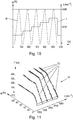
- the identification leads to the parameters ⁇ i of the local models M i that are blended as describes above. From the parameters ⁇ i the parameter maps for the system parameters, here e.g. ⁇ , K and D (if used), are generated. In Fig.14 the three parameter maps for parameters gain K, time constant ⁇ and time delay D are shown. The identified parameters for the different operating points (defined by the testrun) are shown as dots. Again a Gaussian process modelling approach can be used to generate the shown parameter maps from the single dots.
- the feedforward controller 3 of the 2DoF controller 2 is fully parameterized.
- the feedback controller 4 compensates for the model mismatch and provides disturbance rejection. Since the closed loop is linearised by application of the feedforward controller 3, the feedback controller 4 can be simple (e.g. a simple PI- or PID-controller or any other known conventional controller) and does not need to be fine tuned.
- the parameters of the feedback controller 4 can either be preset to reasonable values, which is in most cases sufficient.
- the parameters of the feedback controller 4 can also be tuned, for example using a simple known Ziegler-Nichols tuning method.
- the Ziegler-Nichols method is a well-known heuristic method of tuning a PID or PI controller. It is basically performed by increasing the parameters of the chosen controller until a satisfactory behaviour is reached. It is of course also possible to apply other known methods for designing the feedback controller 4 and/or for tuning the parameters of the feedback controller 4 or to apply different and also more complex control strategies with the feedback controller 4.
- the engine 14 on the testbed 10 passed a standardized emission test cycle testrun as shown in Fig. 15 .
- the 2DoF controller 2 is used to control the engine 14 on the testbed 10 according to the emission test cycle.
- This means that the defined testcycle provides the setpoints y set (torque T dem ) and the 2DoF controller 2 calculates the pedal position ⁇ as control variable u.
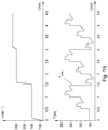
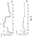
- the results are shown in Fig.16 for a zoomed-in portion of the emission test cycle testrun in which the performance of the inventive controller 2 (curve 30) is compared with the performance of an ENPAC controller (Curve 31) mentioned in the introductory part of the specification. From Fig.16 it is apparent that the inventive controller 2 is able to track the demanded torque T dem better than the ENPAC controller.
Landscapes
- Engineering & Computer Science (AREA)
- Physics & Mathematics (AREA)
- General Physics & Mathematics (AREA)
- Automation & Control Theory (AREA)
- Health & Medical Sciences (AREA)
- Artificial Intelligence (AREA)
- Computer Vision & Pattern Recognition (AREA)
- Evolutionary Computation (AREA)
- Medical Informatics (AREA)
- Software Systems (AREA)
- Feedback Control In General (AREA)
Abstract
Description
- The invention pertains to a method for controlling a technical system as plant with a Two Degree of Freedom controller having a feedforward controller providing an output and a feedback controller providing an output whereas the feedforward controller uses an inverse of the plant and the Two Degree of Freedom controller is designed to calculate a control variable of the plant from the output of the feedforward controller and the output of the feedback controller to achieve a setpoint value of an output variable of the plant in dependence from a state variable of the plant. Furthermore, the invention pertains to the parameterization of the Two Degree of Freedom controller for controlling the technical system.
- There are many applications where a plant has to be controlled using a controller. A plant (also often called controlled system), as expression of control theory, represents the technical system to be controlled. An example of a technical system is an engine testbed on which the engine torque of the internal combustion engine (unit under test on the testbed) has to be controlled in accordance to set reference values (e.g. a demanded torque). The controller has to be designed and/or parameterized to adapt the controller to the static and dynamic behaviour of the actual plant. Only a correctly tuned controller is able to adequately and sufficiently control the plant, e.g. with respect to control error, stability, controllability, etc. Many plants, however, show a (highly) nonlinear dynamic behaviour in practice, which makes the controller design and/or parameterization difficult. Therefore, often a given controller design with a set of controller parameters is used for a given plant or control task which is then only parameterized (assigning values to the controller parameters) by tuning the controller parameters in order to achieve a desired, given control behaviour. Although the controller design can be simple, tuning of the controller parameters has proven to be difficult because of the nonlinear behaviour of the plant. Therefore often highly trained and experienced experts are required to successfully parameterize such a controller. For the engine testbed example, but also for other testbed applications as e.g. for a transmission testbed, drive train testbed, vehicle testbed, roller testbed, etc., an Enhanced Progressive Adaptive Controller (ENPAC) is often used. However, as mentioned before, tuning of an ENPAC is a rather difficult and time consuming task.
- There are of course also other controller designs known. Especially a known Two Degree of Freedom (2DoF) controller is well suited for many applications, as such controller show good reference tracking performance and disturbance rejection. The problem with such a controller is that the controller uses an inversion of the plant in the feedforward part of the controller. For a linear plant, an inversion is usually easy to determine. But this does not apply to a nonlinear plant. Therefore a 2DoF controller cannot easily be used for controlling a nonlinear plant.
- It is therefore an object of the present invention to provide a method for controlling a technical system as nonlinear plant with a Two Degree of Freedom controller and for designing and parameterizing such a Two Degree of Freedom (2DoF) controller for a nonlinear plant, which preferably allows also an automated parameterization of the controller.
- This object is achieved in that the inverse of the plant is constituted by a nonlinear dynamic part and a nonlinear static part, a static map of the plant is provided that maps the control variable and the state variable onto the output variable and the nonlinear static part is formed by an inverse of this static map, whereas the inverse outputs the control variable for a given state variable and output variable, the plant is modelled with a model with a chosen model structure having system parameters and that the nonlinear dynamic part is formed as function of the system parameters of the model and of a desired output variable of a desired closed loop behaviour of the plant and the output of the nonlinear dynamic part and the state variable are fed into the inverse of the static map of the nonlinear static part that outputs the control variable for controlling the plant. With the nonlinear static and nonlinear dynamic part it is possible to approximate the inverse of the nonlinear plant model, which can then be used in the feedforward controller. The nonlinear dynamic part approximates the dynamic behaviour of the plant and the nonlinear static part the static behaviour. By modelling the nonlinear static part as static map it is possible to determine its inverse which is fed by the output of the nonlinear dynamic part.
- This controller can be parameterized by carrying out a first defined testrun on the testbed with the unit under test and by collecting first testrun data during the first testrun which is used to identify the static map of the plant that maps the control variable and the state variable onto the output variable and this static map is inverted to form the nonlinear static part of the feedforward controller, and by carrying out a second defined testrun on the testbed with the unit under test and by collecting second testrun data during the second testrun which is used for identification of the system parameters of the model of the plant for the nonlinear dynamic part. This allows for an easy parameterization of the Two Degree of Freedom controller, or its feedforward controller, with an easy to follow routine that could also be performed fully automatically on the test bed. The feedback controller can be regarded as being parameterized, as its parameters are easy to parameterize or to tune, especially as there are no high demands on the feedback controller.
- The present invention is explained in greater detail below with reference to
Figures 1 to 16 , which show by way of example, schematically and without limitation, advantageous embodiments of the invention. In the drawings: - Fig.1
- the known structure of a 2DoF controller,
- Fig.2
- an example of a technical system in form of an engine testbed as controlled plant,
- Fig.3
- a first order model structure as model of the plant,
- Fig.4
- a desired closed loop behaviour of the plant,
- Fig.5
- a static map of the plant,
- Fig.6
- the monotonization of the static map,
- Fig.7
- the inverse of the static map,
- Fig.8
- an example of the structure of the feedforward controller,
- Fig.9
- the implementation of a time delay in the 2DoF controller,
- Fig.10
- a testrun for identification of the static map,
- Fig.11
- a measured static map during the testrun,
- Fig.12
- a dynamic testrun for identification of the system parameters,
- Fig.13
- the measured response during the dynamic testrun,
- Fig.14
- identified maps of the system parameters,
- Fig.15
- a standardized emission test cycle and
- Fig.16
- the measured response during the standardized emission test cycle.
- In
Fig.1 the general and well known controller structure of a Two Degree of Freedom (2DoF)controller 2 for controlling aplant 1 is shown. The Two Degree of Freedomcontroller 2 comprises afeedforward controller 3 and afeedback controller 4. As it is often impossible to achieve good setpoint tracking and fast disturbance rejection at the same time with an ordinary feedback controller with one degree of freedom, a Two Degree of Freedom (2DoF)controller 2 with two degrees of freedom can be used as is shown inFig.1 . - The
plant 1 is a dynamic technical system that needs to be controlled. The technical system is for example atestbed 10 with a unit undertest 11 arranged and operated on thetestbed 10 as shown inFig.2 . There can also aload machine 13 be arranged on thetestbed 10 which is connected to the unit undertest 11 for applying a load (e.g. a load torque) to the unit undertest 11. Theload machine 13 can also be part of theplant 1. Thetestbed 10 can be an engine testbed with aninternal combustion engine 14 as unit undertest 11 that is connected to a dynamometer (e.g. an electric motor or a water brake dynamometer) asload machine 13. Theplant 1 is controlled with a control variable u calculated by thecontroller 2 which is implemented (software and/or hardware) in aplant control unit 15. The control variable u is e.g. used to adjust at least one actuator of theplant 1. The control variable u of anengine 14 can be the percentage α of the applied throttle pedal, for example. Thecontroller 2 controls an output variable y of theplant 1 according to a given setpoint yset. For anengine 14 the setpoint yset can be a demanded torque TD, for example. Theplant 1, or in general the technical system, responses with the output variable y if the input variable u is applied to theplant 1. The output variable y of anengine 14 is for example the actual engine torque T. The current value of the output variable y can be measured by asuitable sensor 16, e.g. a torque sensor, can be calculated by using a simulation model, e.g. of the unit undertest 11, of a vehicle into which the unit undertest 11 is arranged, etc., or can be estimated with an observer from other known (e.g. by measured) variables of theplant 1. The output variable y is fed back in known manner to thecontroller 2 for feedback control. - For the Two Degree of
Freedom controller 2 as shown inFig.1 , the output variable y is fed back to the input of thefeedback controller 4, to form the control error e as input to thefeedback controller 4. The2DoF controller 2 utilizes usually also certain state variables x of theplant 1, e.g. an engine speed n in case of anengine 14. The state variable x can be measured by using asensor 17, can be calculated by using a simulation model, e.g. of the unit undertest 11, of a vehicle into which the unit undertest 11 is arranged, etc., or can be estimated with an observer for the state variable x from other known (e.g. measured) variables of theplant 1. - The control variable u for the
plant 1 calculated in the2DoF controller 2 comprises a control variable uFF of thefeedforward controller 3 and a control variable uFB of thefeedback controller 4, which are summed to form the control variable u for theplant 1. The setpoint yset is fed to thefeedforward controller 3 and to thefeedback controller 4. The controller design is usually done with a (mathematical) model of theplant 1 that comprises also certain state variables x. The model of theplant 1 maps the input (control variable u) to the output y. There can of course also be more than one output variable y and/or state variable x and are consequently to be understood generally as vectors with dimension ≥1. - In well-known manner, the
feedforward controller 3 embodies an inverse of the controlledplant 1, i.e. an inverse of the model of theplant 1. Unfortunately, the model of a dynamic technical system as theplant 1 is usually nonlinear. As it is difficult to determine the inverse of a nonlinear plant model, the most challenging task of the design of theinventive 2DoF controller 2 is the implementation of thefeedforward controller 3. The necessary inversion of theplant 1 according to the invention is described in the following, without limitation, on the example of a plant model having a known first order model structure. - A first order plant is in general defined as τ·ẏ+y=K·u with the input u, the output y and the time derivative of the output ẏ, which leads to the model structure as shown in
Fig.3 . K is the gain and τ the time constant, which are both given system parameters defined by the implementation of theplant 1 and can be regarded as being known. The known model structure of the first order plant is shown inFig.3 , where s represents the known Laplace operator. In the shown structure C1 and C2 represent input and output offsets, respectively. From the structure inFig.3 the equation
plant 1 is a dynamic technical system, the parameters K and τ, and also C1, C2 if present, are dependent from a current operating point (output variable y and state variable x at a certain point in time) of the dynamic system and the equation is nonlinear and therefore not directly invertible. - For designing the
feedforward controller 3 of the Two Degree ofFreedom controller 2 despite the nonlinear plant model a desired closed loop behaviour of theplant 1 is chosen as shown inFig.4 . The chosen desired behaviour is defined by the desired time constant τdes which produces a desired output variable ydes. It should be noted that the structure of the desired plant (Fig.4 ) is preferably the same as the structure of the plant model (Fig.3 ). I.e., if the response of theplant 1 can be characterized as a first order response, then the desired behaviour is preferably also a first order model, if the plant response is of second order then the desired behaviour is preferably of second order, and so on. Now, by comparison, it is possible to substitute ẏ* and y in above equation of the plant model with ẏdes and ydes of the desired plant which leads to
plant 1. In this equation û is the input variable that would be required to achieve the desired output variable ydes. In other words, if the new input variable û is applied to theplant 1, theplant 1 would response with the desired output variable ydes. From that it is apparent that this equation represents an approximation of the inverse of the plant model with a design parameter τdes or ydes and with the system parameters K, τ of theplant 1. - This can be used to design the
feedforward controller 3. The above equation comprises a nonlinear dynamic part
static part 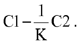
plant 1 and of a desired output variable ydes. - As nonlinear static part a
map 20 of the output variable y in dependence of the control variable u and state variable x is used in accordance with the invention, that is y(k) = f(x(k), u(k)) where k represents the actual time step of the control and f a function that maps the control variably u and state variable x to the output variable y. Such amap 20 is exemplarily shown inFig.5 for the example of an engine map for anengine 14, with the engine torque T as output variable y, the percentage α of the applied throttle pedal as control variable u and the engine speed n as state variable x. The inverse of the nonlinear static part can then be written as û(k) = f-1(x(k), y(k)). For an exact inversion û(k) = u(k) would hold. - If the function f is monotonically increasing over the entire range of the control variable u for a given state variable x, then it is easily possible to determine its inverse, i.e. the function f-1, with known methods. For example the inverse could be found with help of the Matlab (Matlab is a known software of the company The MathWorks) function interp1(), that realises a 1-D data interpolation. This leads to the
inverted map 21 of themap 20. - If the function f is not monotonically increasing over the entire range of the control variable u, however, then a monotonization step is carried out first. The monotonization can be done as described in the following with reference to
Fig.6 . - A
map 20 is usually stored as multidimensional (according to the dimension of the map 20) table with multiple datapoints DP where every datapoint DP has the dimension of themap 20. Then the state variable x is held constant and the function of the output variable y in dependence from the control variable u is analysed. If the output variable y is not monotonically increasing over the entire range of the control variable u, the last datapoint D1 where the function is still monotonically increasing is searched. From this datapoint D1 and the datapoint D2 of the maximum value of the output variable y the slope of a line connecting the datapoints D1 and D2 is calculated. This slope is then added to all the datapoints DP in the region where the output variable y is not monotonically increasing. InFig.6 the dotted line shows the original non-monotonically increasing output variable function f and the solid line shows the resulting monotonized output variable function f. This is repeated for different values of the state variable x in order to obtain the monotonized map 20'. Finally also a known smoothing of the monotonized map 20' can be applied to all the manipulated datapoints DP. In this way a monotonically increasing output variable function f can be guaranteed and the shape of the original function f can basically be preserved. For the inversion step it is important that themap 20 is at least monotonically increasing along the axis of the control variable u (i.e. for a given, fixed state variable x). - The monotonization of the
map 20 introduces of course an additional control error. This error is seen as model mismatch which is compensated for by thefeedback controller 4. - The resulting monotonized map 20' can then be inverted with known means as described above. The final
inverted map 21 of the monotonized map 20' of themap 20 inFig.5 is shown exemplarily inFig.7 . Theinverted map 21 outputs the control variable u (e.g. pedal position α) for a given operating point, given by a state variable x (e.g. speed n) and a given output variable y (e.g. torque T). The above nonlinearstatic part 
map 20 and consequently also in theinverted map 21. - The nonlinear dynamic part

plant 1 as functions of the operating point of the system given by the output variable y and state variable x. For the example of anengine 14 the operating point could be given by the engine torque T and engine speed n. To determine the system parameters τ̇, K the dynamic system is first identified and modelled with a local model network (LMN) that models the nonlinear dynamic behaviour of the system, i.e. theplant 1. LMNs are well-known in the art and calculate an estimation ŷ of the output variable y as a weighted combination of a number i=1,...,m outputs ŷi of local models Mi that are combined to form a global model. The weighing is done with a validity function ρi, which is a function of a scheduling vector Φ that defines the operating point of the system. The scheduling vector is usually a subvector of a data vector ψ=(u, x, y)T. The validity functions ρi define the activation level of local models Mi at a particular operating point (given as scheduling vector Φ). This means that not every local model Mi contributes in every operating point in the same amount to the estimation of the output variable ŷ. The output ŷ of the LMN can generally be written as
- For the local models Mi a suitable model structure is chosen, usually a linear function of the data vector ψ and with local model parameters in form of a parameter vector Θ, although it is also possible to choose a nonlinear function as local Model Mi. For a linear local model Mi the local output ŷi can generally be written as ŷi =Ψ·Θi and the LMN as

- A local model Mi can for example be defined as polynomial according to ŷi(k)=ai1yi(k-1)+...+ainyi(k-n)+...+bi1u(k)+...+bimu(k-m)+di with n past output y and present and m past input u samples. With such a model Mi the data vector ψ follows as Ψ=(y(k-1) ··· y(k-n) u(k) ··· u(k-m) 1)T and the parameter vector Θ as

- In case of a first order model structure, the local model Mi could be given by

- If all local models Mi share the same model structure (which is usually and also in this application the case), the estimation ŷ of the output variable y could also be calculated from the LMN by blending the parameters Θ instead of blending the local outputs ŷi. In this case the LMN can be written as

- For this calculation the identified parameters ain, bim in the discrete time domain could be transformed into the continuous time domain, for example with the help of the well-known bilinear transformation. This leads to parameters a, b for a given operating point in continuous time domain. The parameters K and τ could then be calculated as


Fig.3 . At different operating points a step could be applied as input u to theplant 1 and the output y could be recorded. Then the same input is applied to the chosen model structure and the parameters of the model, here e.g. parameters K and τ, are varied to produce the same output or to optimize, preferably minimize, (according to a given criteria) the cost function (e.g. mean square error) of the difference between the model output and the measured output. By that it is possible to determine the system parameters K and τ for different operating points. - The use of LMNs to model nonlinear systems is well known, e.g. from Gregorcic, G., et al., "Nonlinear system identification: From multiple-model networks to Gaussian processes", Engineering Applications of Artificial Intelligence 21 (2008), p.1035-1055. The identification of a LMN for a given technical system for modelling the technical system is also well documented in the prior art, e.g. in Hametner, C., et al., ,,Local model network identification for online engine modelling", 2013, Information Sciences 220 (0), S.210-225. Basically LMNs are identified from given data from the technical system, e.g. measured data from the technical system. LMNs and its identification are therefore not explained in more detail here.
- By identifying the
plant 1 with a LMN using blended model parameters maps of the system parameters K, τ in dependence from an operating point can be obtained. These system parameter maps for the parameters K, τ can then directly be used in the nonlinear dynamic part
feedforward controller 4. - It would also be possible to use another global model instead of the LMN as long as the global model utilizes model structures according to the model structure of the
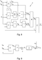
plant 1. This allows identification of the system parameters of theplant 1 with the global model which can then be used to approximate the inverse of the plant model as described above The nonlinear static part and the nonlinear dynamic part need to be combined in order to form the output uFF of thefeedforward controller 3. This is done as described with reference toFig.8 and for the above example of a first order model structure. - The control parameter of the
feedforward controller 4 is the chosen desired behaviour of theplant 1. In the above example of a first order model structure, the design parameter would be the desired time constant τdes (seeFig.4 ). By setting the desired time constant τdes the behaviour of the controlled dynamic system can be affected. In thetrajectory block 5 the desired output ydes and its time derivative ẏdes are calculated in accordance to the chosen desired closed loop behaviour (in the example as shown inFig.4 ). With the (offline and beforehand) identified system parameter maps the system parameters τ, K are determined for the current operating point (given by the state variable x and setpoint yset) which are used to calculate the nonlinear dynamic part
static map 21 which in turn outputs the control variable uFF of thefeedforward controller 3. This means that a shaped dynamic output variable ydyn is input into the invertedstatic map 21 to achieve the desired behaviour of theplant 1. - From the above it is apparent that also other model structures could be used instead of a first order model structure. Another simple model structure could be an also known second order model structure or a polynomial model structure.
- External disturbances and an unavoidable model mismatch (e.g. caused by the inversion of the map or the identification of the parameter maps) are compensated for by the
feedback controller 4 of the2DoF controller 2. - It would also be possible to extend the model structure with a system time delay D which is given by the time that is required for the output y of the system (plant 1) to respond if the input u is changed. Consideration of the time delay D is advantageous to ensure that the
feedback controller 4 is in synchronization with thefeedback controller 3 and the system response. When the output uFF of thefeedforward controller 3 calculated from a new setpoint yset is applied to theplant 1, theplant 1 responds to this input only after the time delay D. But thefeedback controller 4 would immediately react on the new setpoint yset. Therefore, the time delay D is used to delay the setpoint yset before it is fed into the feedback controller 4-The time delay D could also be identified in course of the identification of the LMN and could also be given by a map in dependence from the operating point (output y and state variable x). To this end the time delay D could also be measured during the identification of the LMN. The time delay D could then be used in the2DoF controller 2 4 to delay the desired output ydes that is used in thefeedback controller 4. To this end the output of thetrajectory block 5 of thefeedforward controller 3 can be used, as exemplarily shown inFig.9 . In an alternative implementation the output setpoint yset and the state variable x could directly be used as input of the map for the time delay D. - The parameterisation of the Two Degree of
Freedom controller 2 can be fully automatized for a givenplant 1 as is described in the following. For the parameterisation the model structures of the plant model and of the local models Mi of the LMN are defined, e.g. a first order model structure as described above. The method for parameterisation comprises the identification of the nonlinear static part as map 20 (and its inverse) and of the system parameters of theplant 1 which are required for the nonlinear dynamic part. The order of these identification procedures is not important. - For identification of the nonlinear static part a predefined testrun is carried out with the unit under
test 11 on thetestbed 10. The automatic identification implies of course that thetestbed 10 is fully automatized so that the testrun can be performed without the need of an operator. If this is not the case the support of an operator would be required which would lead to semi-automatic identification. A possible exemplary testrun for identifying an engine map asstatic map 20 of anengine 14 is exemplarily shown inFig.10 . The testrun is advantageously designed to identify the static behaviour of theplant 1, e.g. preferably without transient changes. The testrun comprises a number of speed n (state variable x) steps accompanied with a slow variation of the pedal position α (control variable u) for every speed n step. There are of course also known methods, so called design of experiments DoE, to define a testrun with generates data with optimum information content for identification of a system. The defined testrun is carried out on thetestbed 10 with the unit undertest 11 and the output y (torque T) is measured. For anengine 14 the pedal position α (input variable u) and the engine speed n (state variable x) are varied and the torque T is measured as output y. Part of the generated measured data (training data TD) is used for the identification of themap 20. The rest of the data (or part of the rest of the data can be used for verification). The training data TD is shown inFig.11 with the plus-sign for the example of anengine 14. A Gaussian process approach (e.g. as described in Gregorcic, G., et al., "Gaussian process approach for modelling of nonlinear systems", Engineering Applications of Artificial Intelligence 22 (2009), p.522-533) can be utilised to obtain thestatic map 20 from the training data TD. Thestatic map 20 can then be inverted as described above to obtain theinverted map 21. - For identification of the LMN the number and distribution (validity function ρi) of the local models Mi has to be defined first. For example fifteen local models Mi (three in each speed n step of the
above map 20 identification) could be placed in the regions of the measured data inFig.11 where the engine torque T does not saturate. To identify the LMN another testrun is used, this time a testrun that advantageously allows identification of the local dynamic behaviour of theplant 1. Again DoE methods could be used to define the testrun. A possible testrun is shown inFig. 12 and comprises speed n steps and this time transient changes of pedal position α for every speed n step. The testrun should of course be designed to stimulate theplant 1 in the region of the operating points the local models Mi are placed. This dynamic testrun is again automatically, or semi-automatically, run on thetestbed 10 with the unit undertest 11. The measured response (output y for the varying input u and a given state x) for the testrun ofFig.12 is shown inFig.13 . The collected data of the testrun (measured torque T) is then split in training data and validation data and the training data is used for identification of the LMN, e.g. as described in Hametner, C., et al., "Local model network identification for online engine modelling", 2013, Information Sciences 220 (0), S.210-225. - When the testrun is designed with sequences that especially stimulate single local models Mi (as in
Fig.12 ), the collected data could also be divided in single sequences. Every sequence can then be used to identify the local model Mi assigned to this sequence. The sequence Sn inFig.13 is for example used to identify the n-th local model Mn, and so on. - The identification leads to the parameters Θi of the local models Mi that are blended as describes above. From the parameters Θi the parameter maps for the system parameters, here e.g. τ, K and D (if used), are generated. In
Fig.14 the three parameter maps for parameters gain K, time constant τ and time delay D are shown. The identified parameters for the different operating points (defined by the testrun) are shown as dots. Again a Gaussian process modelling approach can be used to generate the shown parameter maps from the single dots. - With the parameter maps (
Fig.14 ) and thestatic map 20, or its inverse, thefeedforward controller 3 of the2DoF controller 2 is fully parameterized. - The
feedback controller 4 compensates for the model mismatch and provides disturbance rejection. Since the closed loop is linearised by application of thefeedforward controller 3, thefeedback controller 4 can be simple (e.g. a simple PI- or PID-controller or any other known conventional controller) and does not need to be fine tuned. The parameters of thefeedback controller 4 can either be preset to reasonable values, which is in most cases sufficient. The parameters of thefeedback controller 4 can also be tuned, for example using a simple known Ziegler-Nichols tuning method. The Ziegler-Nichols method is a well-known heuristic method of tuning a PID or PI controller. It is basically performed by increasing the parameters of the chosen controller until a satisfactory behaviour is reached. It is of course also possible to apply other known methods for designing thefeedback controller 4 and/or for tuning the parameters of thefeedback controller 4 or to apply different and also more complex control strategies with thefeedback controller 4. - To verify the design of the
2DoF controller 2 theengine 14 on thetestbed 10 passed a standardized emission test cycle testrun as shown inFig. 15 . The2DoF controller 2 is used to control theengine 14 on thetestbed 10 according to the emission test cycle. This means that the defined testcycle provides the setpoints yset (torque Tdem) and the2DoF controller 2 calculates the pedal position α as control variable u. The results are shown inFig.16 for a zoomed-in portion of the emission test cycle testrun in which the performance of the inventive controller 2 (curve 30) is compared with the performance of an ENPAC controller (Curve 31) mentioned in the introductory part of the specification. FromFig.16 it is apparent that theinventive controller 2 is able to track the demanded torque Tdem better than the ENPAC controller.
Claims (9)
- Method for controlling a technical system as plant (1) with a Two Degree of Freedom controller (2) having a feedforward controller (3) providing a first output (uFF) and a feedback controller (4) providing a second output (uFB) whereas the feedforward controller (3) uses an inverse of the plant (1) and the Two Degree of Freedom controller (2) is designed to calculate a control variable (u) of the plant (1) from the first output (uFF) of the feedforward controller (3) and the second output (uFB) of the feedback controller (4) to achieve a setpoint value (yset) of an output variable (y) of the plant (1) in dependence from a state variable (x) of the plant (1), characterized in that the inverse of the plant (1) is constituted by a nonlinear dynamic part and a nonlinear static part, that a static map (20) of the plant (1) is provided that maps the control variable (u) and the state variable (x) onto the output variable (y) and the nonlinear static part is formed as inverted map (21) of this static map (20), whereas the inverted map (21) outputs the control variable (u) for a given state variable (x) and output variable (y), that the plant (1) is modelled with a model with a chosen model structure having system parameters (K, τ) and that the nonlinear dynamic part is formed as function of the system parameters (K, τ) of the model and of a desired output variable (ydes) of a desired closed loop behaviour of the plant (1) and that the dynamic output (ydyn) of the nonlinear dynamic part and the state variable (x) are fed into the inverted map (21) of the nonlinear static part that outputs the first output (uFF) of the feedforward controller (3).
- Method according to claim 1, characterized in that the plant (1) is modelled as first order plant with a gain (K) and a time constant (τ) as system parameters.
- Method according to claim 1, characterized in that the setpoint value of the output variable (yset) or the desired output variable (ydes) is delayed by a system time delay (D) before it is fed into the feedback controller (4).
- Method for parameterization of a Two Degree of Freedom controller (2) used for controlling a technical system with a testbed (10) and a unit under test (11) arranged on the testbed (10) as plant (1), whereas the Two Degree of Freedom controller (2) comprises a feedforward controller (3) and a feedback controller (4) and the feedforward controller (3) embodies an inverse of the plant (1) which is constituted by a nonlinear dynamic part and a nonlinear static part, whereas- a first defined testrun is carried out on the testbed (10) with the unit under test (11) and first testrun data is collected during the first testrun and the collected first testrun data is used to identify a static map (20) of the plant (1) that maps a control variable (u) and a state variable (x) onto an output variable (y) of the plant (1) and this static map (20) is inverted to a inverted static map (21) which represents the nonlinear static part of the feedforward controller (3), and- a second defined testrun is carried out on the testbed (10) with the unit under test (11) and second testrun data is collected during the second testrun and the collected second testrun data is used for identification of the system parameters (K, τ) of a model of the plant (1), which represents the nonlinear dynamic part.
- Method according to claim 4, characterized in that the identified static map (20) is monotonized before its inversion.
- Method according to claim 5, characterized in that for monotonization for at least one constant state variable (x) a first datapoint (D1) is searched as the last datapoint (DP) for which the output variable (y) is still monotonically increasing in dependence from the control variable (u), and in that a second datapoint (D2) of the maximum value of the output variable (y) is searched and the slope of a line connecting the first datapoint (D1) and the second datapoint (D2) is calculated and this slope is added to all datapoints (DP) in the region where the output variable (y) is not monotonically increasing.
- Method according to claim 4, characterized in that a local model network that models the nonlinear dynamic behaviour of the plant (1) is identified with the collected second testrun data and the system parameters (K, τ) are determined from the parameters (a, b) of the local model network.
- Method according to claim 7, characterized in that the system parameters (K, τ) are identified as parameter maps mapping the output variable (y) and the state variable (x) onto the system parameters (K, τ).
- Method according to claims 7 or 8, characterized in that a system time delay (D) is determined as further system parameter.
Priority Applications (1)
| Application Number | Priority Date | Filing Date | Title |
|---|---|---|---|
| EP16201898.0A EP3330812B1 (en) | 2016-12-02 | 2016-12-02 | Method for controlling a technical system with a two degree of freedom controller and its parameterization |
Applications Claiming Priority (1)
| Application Number | Priority Date | Filing Date | Title |
|---|---|---|---|
| EP16201898.0A EP3330812B1 (en) | 2016-12-02 | 2016-12-02 | Method for controlling a technical system with a two degree of freedom controller and its parameterization |
Publications (2)
| Publication Number | Publication Date |
|---|---|
| EP3330812A1 true EP3330812A1 (en) | 2018-06-06 |
| EP3330812B1 EP3330812B1 (en) | 2021-10-27 |
Family
ID=57754919
Family Applications (1)
| Application Number | Title | Priority Date | Filing Date |
|---|---|---|---|
| EP16201898.0A Active EP3330812B1 (en) | 2016-12-02 | 2016-12-02 | Method for controlling a technical system with a two degree of freedom controller and its parameterization |
Country Status (1)
| Country | Link |
|---|---|
| EP (1) | EP3330812B1 (en) |
Cited By (4)
| Publication number | Priority date | Publication date | Assignee | Title |
|---|---|---|---|---|
| CN114755914A (en) * | 2022-04-11 | 2022-07-15 | 中国航发控制系统研究所 | Aero-engine servo controller design method based on IMC-PID |
| DE102023111180B4 (en) | 2022-05-03 | 2024-05-16 | Avl List Gmbh | Method for identifying a law for the feedforward control of a control parameter of a powertrain from measurement data |
| EP4686985A1 (en) * | 2024-08-01 | 2026-02-04 | ABB Schweiz AG | Control method and control device with anomaly detection |
| CN122411077A (en) * | 2026-06-15 | 2026-07-17 | 福建睿斯科医疗技术有限公司 | Method and system for controlling beam current track of accelerator based on neural network inverse model |
Citations (2)
| Publication number | Priority date | Publication date | Assignee | Title |
|---|---|---|---|---|
| US20060241786A1 (en) * | 1996-05-06 | 2006-10-26 | Eugene Boe | Method and apparatus for approximating gains in dynamic and steady-state processes for prediction, control, and optimization |
| CN1877105B (en) * | 2006-06-30 | 2012-02-08 | 清华大学 | Automobile longitudinal acceleration tracking control method |
-
2016
- 2016-12-02 EP EP16201898.0A patent/EP3330812B1/en active Active
Patent Citations (2)
| Publication number | Priority date | Publication date | Assignee | Title |
|---|---|---|---|---|
| US20060241786A1 (en) * | 1996-05-06 | 2006-10-26 | Eugene Boe | Method and apparatus for approximating gains in dynamic and steady-state processes for prediction, control, and optimization |
| CN1877105B (en) * | 2006-06-30 | 2012-02-08 | 清华大学 | Automobile longitudinal acceleration tracking control method |
Non-Patent Citations (5)
| Title |
|---|
| BINGZHAO GAO ET AL: "Position Control of Electric Clutch Actuator Using a Triple-Step Nonlinear Method", IEEE TRANSACTIONS ON INDUSTRIAL ELECTRONICS., vol. 61, no. 12, 1 December 2014 (2014-12-01), USA, pages 6995 - 7003, XP055375697, ISSN: 0278-0046, DOI: 10.1109/TIE.2014.2317131 * |
| GREGORCIC, G. ET AL.: "Gaussian process approach for modelling of nonlinear systems", ENGINEERING APPLICATIONS OF ARTIFICIAL INTELLIGENCE, vol. 22, 2009, pages 522 - 533 |
| GREGORCIC, G. ET AL.: "Nonlinear system identification: From multiple-model networks to Gaussian processes", ENGINEERING APPLICATIONS OF ARTIFICIAL INTELLIGENCE, vol. 21, 2008, pages 1035 - 1055 |
| HAMETNER, C. ET AL.: "Local model network identification for online engine modelling", INFORMATION SCIENCES, vol. 220, no. 0, 2013, pages 210 - 225 |
| PRODROMOS DAOUTIDIS ET AL: "Synthesis of FeedforwardIState Feedback Controllers for Nonlinear Processes", AICHE JOURNAL, 1 October 1989 (1989-10-01), pages 1602 - 1616, XP055376265, Retrieved from the Internet <URL:https://deepblue.lib.umich.edu/bitstream/handle/2027.42/37404/690351004_ftp.pdf;sequence=1> [retrieved on 20170526] * |
Cited By (4)
| Publication number | Priority date | Publication date | Assignee | Title |
|---|---|---|---|---|
| CN114755914A (en) * | 2022-04-11 | 2022-07-15 | 中国航发控制系统研究所 | Aero-engine servo controller design method based on IMC-PID |
| DE102023111180B4 (en) | 2022-05-03 | 2024-05-16 | Avl List Gmbh | Method for identifying a law for the feedforward control of a control parameter of a powertrain from measurement data |
| EP4686985A1 (en) * | 2024-08-01 | 2026-02-04 | ABB Schweiz AG | Control method and control device with anomaly detection |
| CN122411077A (en) * | 2026-06-15 | 2026-07-17 | 福建睿斯科医疗技术有限公司 | Method and system for controlling beam current track of accelerator based on neural network inverse model |
Also Published As
| Publication number | Publication date |
|---|---|
| EP3330812B1 (en) | 2021-10-27 |
Similar Documents
| Publication | Publication Date | Title |
|---|---|---|
| EP3330812B1 (en) | Method for controlling a technical system with a two degree of freedom controller and its parameterization | |
| CN109976145B (en) | Method for adjusting PID parameters, main controller and storage medium | |
| Sekine et al. | MPC for artificial muscles using FRIT based optimized pseudo linearization model | |
| Jarvis et al. | Stabilizing global mean surface temperature: A feedback control perspective | |
| Sawyer | Gain-scheduled control of a quadcopter UAV | |
| Fuh et al. | Adaptive parameter identification of servo control systems with noise and high-frequency uncertainties | |
| Albin et al. | Nonlinear mpc for combustion engine control: A parameter study for realizing real-time feasibility | |
| Shafiq et al. | U-model-based internal model control for non-linear dynamic plants | |
| Lamara et al. | High dynamic engine-dynamometer identification and control | |
| Wicher et al. | Tuning optimization of extended state observer for two mass system with elastic joint and backlash | |
| Alkhafaji et al. | Proposed a novel method for optimization DC motor controller | |
| Kaur et al. | H-infinity controller design for pneumatic servosystem: a comparative study | |
| Ladaci et al. | Fractional order self-tuning control | |
| Horn et al. | Second-order sliding mode control of electronic throttle valves | |
| Ruderman et al. | Extended SDRE control of 1-DOF robotic manipulator with nonlinearities | |
| Zubkov et al. | Method for Controlling Tracking Actuator | |
| CN104806302A (en) | Steam turbine generator main steam valve opening degree prediction control method based on non-linear interference observer | |
| Shi et al. | Process-model-free design of MPC via a reference-model-based PI controller for the gas turbine | |
| Chou et al. | Design of PID controllers using genetic algorithms approach for low damping, slow response plants | |
| Montanez et al. | Comparison of model predictive control techniques for active suspension | |
| Bosche et al. | A robust analysis approach for a class of uncertain BPV systems | |
| Santoso et al. | Control Strategy Design for DC Motor Speed Regulation Using PID Controller | |
| Sato et al. | Improvement of tracking performance in designing a GPC‐based PID controller using a time‐varying proportional gain | |
| AYDOĞDU et al. | Adaptive control of a time-varying rotary servo system using a fuzzy model reference learning controller with variable adaptation gain | |
| Nezamzadeh et al. | Fault Tolerant Control of Synchronous Generator Using a New MPC Controller Approach |
Legal Events
| Date | Code | Title | Description |
|---|---|---|---|
| PUAI | Public reference made under article 153(3) epc to a published international application that has entered the european phase |
Free format text: ORIGINAL CODE: 0009012 |
|
| STAA | Information on the status of an ep patent application or granted ep patent |
Free format text: STATUS: THE APPLICATION HAS BEEN PUBLISHED |
|
| AK | Designated contracting states |
Kind code of ref document: A1 Designated state(s): AL AT BE BG CH CY CZ DE DK EE ES FI FR GB GR HR HU IE IS IT LI LT LU LV MC MK MT NL NO PL PT RO RS SE SI SK SM TR |
|
| AX | Request for extension of the european patent |
Extension state: BA ME |
|
| STAA | Information on the status of an ep patent application or granted ep patent |
Free format text: STATUS: REQUEST FOR EXAMINATION WAS MADE |
|
| 17P | Request for examination filed |
Effective date: 20181205 |
|
| RBV | Designated contracting states (corrected) |
Designated state(s): AL AT BE BG CH CY CZ DE DK EE ES FI FR GB GR HR HU IE IS IT LI LT LU LV MC MK MT NL NO PL PT RO RS SE SI SK SM TR |
|
| RAP1 | Party data changed (applicant data changed or rights of an application transferred) |
Owner name: AVL LIST GMBH |
|
| GRAP | Despatch of communication of intention to grant a patent |
Free format text: ORIGINAL CODE: EPIDOSNIGR1 |
|
| STAA | Information on the status of an ep patent application or granted ep patent |
Free format text: STATUS: GRANT OF PATENT IS INTENDED |
|
| INTG | Intention to grant announced |
Effective date: 20210531 |
|
| GRAS | Grant fee paid |
Free format text: ORIGINAL CODE: EPIDOSNIGR3 |
|
| GRAA | (expected) grant |
Free format text: ORIGINAL CODE: 0009210 |
|
| STAA | Information on the status of an ep patent application or granted ep patent |
Free format text: STATUS: THE PATENT HAS BEEN GRANTED |
|
| AK | Designated contracting states |
Kind code of ref document: B1 Designated state(s): AL AT BE BG CH CY CZ DE DK EE ES FI FR GB GR HR HU IE IS IT LI LT LU LV MC MK MT NL NO PL PT RO RS SE SI SK SM TR |
|
| REG | Reference to a national code |
Ref country code: GB Ref legal event code: FG4D |
|
| REG | Reference to a national code |
Ref country code: CH Ref legal event code: EP |
|
| REG | Reference to a national code |
Ref country code: DE Ref legal event code: R096 Ref document number: 602016065351 Country of ref document: DE |
|
| REG | Reference to a national code |
Ref country code: AT Ref legal event code: REF Ref document number: 1442323 Country of ref document: AT Kind code of ref document: T Effective date: 20211115 |
|
| REG | Reference to a national code |
Ref country code: IE Ref legal event code: FG4D |
|
| REG | Reference to a national code |
Ref country code: LT Ref legal event code: MG9D |
|
| REG | Reference to a national code |
Ref country code: NL Ref legal event code: MP Effective date: 20211027 |
|
| PG25 | Lapsed in a contracting state [announced via postgrant information from national office to epo] |
Ref country code: RS Free format text: LAPSE BECAUSE OF FAILURE TO SUBMIT A TRANSLATION OF THE DESCRIPTION OR TO PAY THE FEE WITHIN THE PRESCRIBED TIME-LIMIT Effective date: 20211027 Ref country code: LT Free format text: LAPSE BECAUSE OF FAILURE TO SUBMIT A TRANSLATION OF THE DESCRIPTION OR TO PAY THE FEE WITHIN THE PRESCRIBED TIME-LIMIT Effective date: 20211027 Ref country code: FI Free format text: LAPSE BECAUSE OF FAILURE TO SUBMIT A TRANSLATION OF THE DESCRIPTION OR TO PAY THE FEE WITHIN THE PRESCRIBED TIME-LIMIT Effective date: 20211027 Ref country code: BG Free format text: LAPSE BECAUSE OF FAILURE TO SUBMIT A TRANSLATION OF THE DESCRIPTION OR TO PAY THE FEE WITHIN THE PRESCRIBED TIME-LIMIT Effective date: 20220127 |
|
| PG25 | Lapsed in a contracting state [announced via postgrant information from national office to epo] |
Ref country code: IS Free format text: LAPSE BECAUSE OF FAILURE TO SUBMIT A TRANSLATION OF THE DESCRIPTION OR TO PAY THE FEE WITHIN THE PRESCRIBED TIME-LIMIT Effective date: 20220227 Ref country code: SE Free format text: LAPSE BECAUSE OF FAILURE TO SUBMIT A TRANSLATION OF THE DESCRIPTION OR TO PAY THE FEE WITHIN THE PRESCRIBED TIME-LIMIT Effective date: 20211027 Ref country code: PT Free format text: LAPSE BECAUSE OF FAILURE TO SUBMIT A TRANSLATION OF THE DESCRIPTION OR TO PAY THE FEE WITHIN THE PRESCRIBED TIME-LIMIT Effective date: 20220228 Ref country code: PL Free format text: LAPSE BECAUSE OF FAILURE TO SUBMIT A TRANSLATION OF THE DESCRIPTION OR TO PAY THE FEE WITHIN THE PRESCRIBED TIME-LIMIT Effective date: 20211027 Ref country code: NO Free format text: LAPSE BECAUSE OF FAILURE TO SUBMIT A TRANSLATION OF THE DESCRIPTION OR TO PAY THE FEE WITHIN THE PRESCRIBED TIME-LIMIT Effective date: 20220127 Ref country code: NL Free format text: LAPSE BECAUSE OF FAILURE TO SUBMIT A TRANSLATION OF THE DESCRIPTION OR TO PAY THE FEE WITHIN THE PRESCRIBED TIME-LIMIT Effective date: 20211027 Ref country code: LV Free format text: LAPSE BECAUSE OF FAILURE TO SUBMIT A TRANSLATION OF THE DESCRIPTION OR TO PAY THE FEE WITHIN THE PRESCRIBED TIME-LIMIT Effective date: 20211027 Ref country code: HR Free format text: LAPSE BECAUSE OF FAILURE TO SUBMIT A TRANSLATION OF THE DESCRIPTION OR TO PAY THE FEE WITHIN THE PRESCRIBED TIME-LIMIT Effective date: 20211027 Ref country code: GR Free format text: LAPSE BECAUSE OF FAILURE TO SUBMIT A TRANSLATION OF THE DESCRIPTION OR TO PAY THE FEE WITHIN THE PRESCRIBED TIME-LIMIT Effective date: 20220128 Ref country code: ES Free format text: LAPSE BECAUSE OF FAILURE TO SUBMIT A TRANSLATION OF THE DESCRIPTION OR TO PAY THE FEE WITHIN THE PRESCRIBED TIME-LIMIT Effective date: 20211027 |
|
| REG | Reference to a national code |
Ref country code: DE Ref legal event code: R097 Ref document number: 602016065351 Country of ref document: DE |
|
| PG25 | Lapsed in a contracting state [announced via postgrant information from national office to epo] |
Ref country code: SM Free format text: LAPSE BECAUSE OF FAILURE TO SUBMIT A TRANSLATION OF THE DESCRIPTION OR TO PAY THE FEE WITHIN THE PRESCRIBED TIME-LIMIT Effective date: 20211027 Ref country code: SK Free format text: LAPSE BECAUSE OF FAILURE TO SUBMIT A TRANSLATION OF THE DESCRIPTION OR TO PAY THE FEE WITHIN THE PRESCRIBED TIME-LIMIT Effective date: 20211027 Ref country code: RO Free format text: LAPSE BECAUSE OF FAILURE TO SUBMIT A TRANSLATION OF THE DESCRIPTION OR TO PAY THE FEE WITHIN THE PRESCRIBED TIME-LIMIT Effective date: 20211027 Ref country code: MC Free format text: LAPSE BECAUSE OF FAILURE TO SUBMIT A TRANSLATION OF THE DESCRIPTION OR TO PAY THE FEE WITHIN THE PRESCRIBED TIME-LIMIT Effective date: 20211027 Ref country code: EE Free format text: LAPSE BECAUSE OF FAILURE TO SUBMIT A TRANSLATION OF THE DESCRIPTION OR TO PAY THE FEE WITHIN THE PRESCRIBED TIME-LIMIT Effective date: 20211027 Ref country code: DK Free format text: LAPSE BECAUSE OF FAILURE TO SUBMIT A TRANSLATION OF THE DESCRIPTION OR TO PAY THE FEE WITHIN THE PRESCRIBED TIME-LIMIT Effective date: 20211027 Ref country code: CZ Free format text: LAPSE BECAUSE OF FAILURE TO SUBMIT A TRANSLATION OF THE DESCRIPTION OR TO PAY THE FEE WITHIN THE PRESCRIBED TIME-LIMIT Effective date: 20211027 |
|
| REG | Reference to a national code |
Ref country code: CH Ref legal event code: PL |
|
| PLBE | No opposition filed within time limit |
Free format text: ORIGINAL CODE: 0009261 |
|
| STAA | Information on the status of an ep patent application or granted ep patent |
Free format text: STATUS: NO OPPOSITION FILED WITHIN TIME LIMIT |
|
| REG | Reference to a national code |
Ref country code: BE Ref legal event code: MM Effective date: 20211231 |
|
| 26N | No opposition filed |
Effective date: 20220728 |
|
| PG25 | Lapsed in a contracting state [announced via postgrant information from national office to epo] |
Ref country code: LU Free format text: LAPSE BECAUSE OF NON-PAYMENT OF DUE FEES Effective date: 20211202 Ref country code: IE Free format text: LAPSE BECAUSE OF NON-PAYMENT OF DUE FEES Effective date: 20211202 Ref country code: AL Free format text: LAPSE BECAUSE OF FAILURE TO SUBMIT A TRANSLATION OF THE DESCRIPTION OR TO PAY THE FEE WITHIN THE PRESCRIBED TIME-LIMIT Effective date: 20211027 |
|
| PG25 | Lapsed in a contracting state [announced via postgrant information from national office to epo] |
Ref country code: SI Free format text: LAPSE BECAUSE OF FAILURE TO SUBMIT A TRANSLATION OF THE DESCRIPTION OR TO PAY THE FEE WITHIN THE PRESCRIBED TIME-LIMIT Effective date: 20211027 Ref country code: BE Free format text: LAPSE BECAUSE OF NON-PAYMENT OF DUE FEES Effective date: 20211231 |
|
| PG25 | Lapsed in a contracting state [announced via postgrant information from national office to epo] |
Ref country code: LI Free format text: LAPSE BECAUSE OF NON-PAYMENT OF DUE FEES Effective date: 20211231 Ref country code: CH Free format text: LAPSE BECAUSE OF NON-PAYMENT OF DUE FEES Effective date: 20211231 |
|
| PG25 | Lapsed in a contracting state [announced via postgrant information from national office to epo] |
Ref country code: HU Free format text: LAPSE BECAUSE OF FAILURE TO SUBMIT A TRANSLATION OF THE DESCRIPTION OR TO PAY THE FEE WITHIN THE PRESCRIBED TIME-LIMIT; INVALID AB INITIO Effective date: 20161202 |
|
| P01 | Opt-out of the competence of the unified patent court (upc) registered |
Effective date: 20230502 |
|
| PG25 | Lapsed in a contracting state [announced via postgrant information from national office to epo] |
Ref country code: CY Free format text: LAPSE BECAUSE OF FAILURE TO SUBMIT A TRANSLATION OF THE DESCRIPTION OR TO PAY THE FEE WITHIN THE PRESCRIBED TIME-LIMIT Effective date: 20211027 |
|
| REG | Reference to a national code |
Ref country code: AT Ref legal event code: UEP Ref document number: 1442323 Country of ref document: AT Kind code of ref document: T Effective date: 20211027 |
|
| PG25 | Lapsed in a contracting state [announced via postgrant information from national office to epo] |
Ref country code: MK Free format text: LAPSE BECAUSE OF FAILURE TO SUBMIT A TRANSLATION OF THE DESCRIPTION OR TO PAY THE FEE WITHIN THE PRESCRIBED TIME-LIMIT Effective date: 20211027 |
|
| PG25 | Lapsed in a contracting state [announced via postgrant information from national office to epo] |
Ref country code: TR Free format text: LAPSE BECAUSE OF FAILURE TO SUBMIT A TRANSLATION OF THE DESCRIPTION OR TO PAY THE FEE WITHIN THE PRESCRIBED TIME-LIMIT Effective date: 20211027 |
|
| PG25 | Lapsed in a contracting state [announced via postgrant information from national office to epo] |
Ref country code: MT Free format text: LAPSE BECAUSE OF FAILURE TO SUBMIT A TRANSLATION OF THE DESCRIPTION OR TO PAY THE FEE WITHIN THE PRESCRIBED TIME-LIMIT Effective date: 20211027 |
|
| PGFP | Annual fee paid to national office [announced via postgrant information from national office to epo] |
Ref country code: GB Payment date: 20251218 Year of fee payment: 10 |
|
| PGFP | Annual fee paid to national office [announced via postgrant information from national office to epo] |
Ref country code: AT Payment date: 20251215 Year of fee payment: 10 |
|
| PGFP | Annual fee paid to national office [announced via postgrant information from national office to epo] |
Ref country code: FR Payment date: 20251217 Year of fee payment: 10 |
|
| PGFP | Annual fee paid to national office [announced via postgrant information from national office to epo] |
Ref country code: DE Payment date: 20251222 Year of fee payment: 10 |
|
| PGFP | Annual fee paid to national office [announced via postgrant information from national office to epo] |
Ref country code: IT Payment date: 20251231 Year of fee payment: 10 |