EP3163771A1 - Method for nonlinear fourier analysis in optical transmission systems - Google Patents

Method for nonlinear fourier analysis in optical transmission systems Download PDF

Info

Publication number
EP3163771A1
EP3163771A1 EP15306711.1A EP15306711A EP3163771A1 EP 3163771 A1 EP3163771 A1 EP 3163771A1 EP 15306711 A EP15306711 A EP 15306711A EP 3163771 A1 EP3163771 A1 EP 3163771A1
Authority
EP
European Patent Office
Prior art keywords
spectral
waveform
function
nonlinear
matrix
Prior art date
Legal status (The legal status is an assumption and is not a legal conclusion. Google has not performed a legal analysis and makes no representation as to the accuracy of the status listed.)
Withdrawn
Application number
EP15306711.1A
Other languages
German (de)
French (fr)
Inventor
Vahid Aref
Henning Bülow
Current Assignee (The listed assignees may be inaccurate. Google has not performed a legal analysis and makes no representation or warranty as to the accuracy of the list.)
Alcatel Lucent SAS
Original Assignee
Alcatel Lucent SAS
Priority date (The priority date is an assumption and is not a legal conclusion. Google has not performed a legal analysis and makes no representation as to the accuracy of the date listed.)
Filing date
Publication date
Application filed by Alcatel Lucent SAS filed Critical Alcatel Lucent SAS
Priority to EP15306711.1A priority Critical patent/EP3163771A1/en
Publication of EP3163771A1 publication Critical patent/EP3163771A1/en
Withdrawn legal-status Critical Current

Links

Images

Classifications

    • HELECTRICITY
    • H04ELECTRIC COMMUNICATION TECHNIQUE
    • H04BTRANSMISSION
    • H04B10/00Transmission systems employing electromagnetic waves other than radio-waves, e.g. infrared, visible or ultraviolet light, or employing corpuscular radiation, e.g. quantum communication
    • H04B10/50Transmitters
    • H04B10/508Pulse generation, e.g. generation of solitons
    • HELECTRICITY
    • H04ELECTRIC COMMUNICATION TECHNIQUE
    • H04BTRANSMISSION
    • H04B10/00Transmission systems employing electromagnetic waves other than radio-waves, e.g. infrared, visible or ultraviolet light, or employing corpuscular radiation, e.g. quantum communication
    • H04B10/25Arrangements specific to fibre transmission
    • H04B10/2507Arrangements specific to fibre transmission for the reduction or elimination of distortion or dispersion
    • H04B10/25077Arrangements specific to fibre transmission for the reduction or elimination of distortion or dispersion using soliton propagation
    • HELECTRICITY
    • H04ELECTRIC COMMUNICATION TECHNIQUE
    • H04BTRANSMISSION
    • H04B10/00Transmission systems employing electromagnetic waves other than radio-waves, e.g. infrared, visible or ultraviolet light, or employing corpuscular radiation, e.g. quantum communication
    • H04B10/60Receivers
    • H04B10/66Non-coherent receivers, e.g. using direct detection
    • HELECTRICITY
    • H04ELECTRIC COMMUNICATION TECHNIQUE
    • H04LTRANSMISSION OF DIGITAL INFORMATION, e.g. TELEGRAPHIC COMMUNICATION
    • H04L27/00Modulated-carrier systems
    • H04L27/26Systems using multi-frequency codes
    • H04L27/2601Multicarrier modulation systems
    • H04L27/2626Arrangements specific to the transmitter only
    • H04L27/2627Modulators
    • H04L27/2628Inverse Fourier transform modulators, e.g. inverse fast Fourier transform [IFFT] or inverse discrete Fourier transform [IDFT] modulators

Definitions

  • This application relates to transmitters and receivers for optical transmission systems using a nonlinear channel, particularly for modulation over nonlinear spectrum including nonlinear frequency division multiplexing (NFDM).
  • NFDM nonlinear frequency division multiplexing
  • Nonlinear Schrödinger equation characterizes the interplay between dispersion and Kerr nonlinearity in the transmission channel and that NLSE can be therefore used to model signal propagation in an optical fiber.
  • NFT nonlinear Fourier transform
  • NFDM nonlinear frequency division multiplexing
  • NFDM nonlinear frequency division multiplexing
  • a nonlinear-dispersive fiber is a favorable "linear" channel in nonlinear spectral domain.
  • the information is modulated over nonlinear spectrum and is transformed to a waveform in time domain via Inverse Nonlinear Fourier Transform (INFT).
  • IFT Inverse Nonlinear Fourier Transform
  • the waveforms which are transformed nonlinearly in time domain have linear transformations in nonlinear Fourier spectrum.
  • the changes of waveforms can be easily tracked in nonlinear spectral domain, i.e. the distortion of the waveforms caused by both fiber nonlinearity and dispersion can be easily analyzed and compensated in spectral domain, which motivates to first modulate information in nonlinear spectrum and then to map, via INFT, the nonlinear spectrum to the corresponding optical fields in time domain.
  • the optical fields are subsequently propagating in an optical fiber causing waveform distortion of the optical fields.
  • the nonlinearly distorted waveforms can be successfully detected by a Nonlinear Fourier Transform (NFT) algorithm at a receiver from corresponding nonlinear spectrum.
  • NFT Nonlinear Fourier Transform
  • the information can be retrieved from the nonlinear spectrum of the received optical fields computed by NFT.
  • NFT Nonlinear Fourier Transform
  • the main reason of modulating information in nonlinear spectrum is that the equivalent channel in nonlinear spectral domain is linear and the information can be retrieved by applying linear filters/equalizers.
  • the nonlinear spectrum can be divided into two parts: the continuous spectrum, corresponding to the "dispersive” signal components, and the discrete spectrum, corresponding to the "solitonic" (non-dispersive) signal components.
  • the discrete spectrum is characterized by ( ⁇ i , Q d ( ⁇ i )) where ⁇ i is an isolated "nonlinear frequency" in upper complex plane, i.e. the eigenvalue of Lax operator, and Q d ( ⁇ i ) is the discrete spectral modulation function at ⁇ i , i.e. the spectral amplitude at this eigenvalue.
  • INFT can be computed by solving a Riemann-Hilbert system of algebraic equations.
  • the computational complexity of the method grows cubic in terms of the number of eigenvalues of discrete spectrum. For instance, if the discrete nonlinear spectrum comprises N pairs: ( ⁇ i , Q d ( ⁇ i )), i.e. there are N non-zero eigenvalues (in the positive complex plane), one needs to inverse a matrix of size N for each signal sample. Therefore, the complexity scales O ( N 2.80 ) per sample. Alternatively, Darboux transform (DT) which has the complexity O ( N 2 ) can be used.
  • a multi-soliton signal can be generated from given eigenvalues ⁇ i but it is not known how to design a signal if the desired spectral amplitudes Q d ( ⁇ i ) shall also be included.
  • the method needs additional 2 N initial parameters which determine the spectral amplitudes. It is not yet known how to choose these initial parameters for the desired spectral amplitudes.
  • the nonlinear Fourier transform is usually defined based on the Zakharov-Shabat system.
  • the pulse q(t) can be represented by N samples.
  • the nonlinear spectrum can be numerically computed by numerical methods such as Forward discretization, Crank-Nicolson method, Layer-peeling method and Ablowitz-Ladick discretization.
  • most of these methods converge slowly and show unacceptable numerical error in estimating discrete spectra when N is not very large.
  • a better estimation like Layer-peeling algorithm usually results in higher computational complexity.
  • the present application proposes a more stable and numerically more precise algorithm to be used in an optical transmitter and an optical receiver of a nonlinear optical transmission system.
  • the present document proposes methods and devices having the features of the respective independent claims for generating at least one waveform in an optical transmission system having a nonlinear-dispersive channel, where the at least one waveform is generated based on at least one spectral modulation function, each spectral modulation function depending on a spectral value, and for detecting at least one waveform having a nonlinear spectrum received via the nonlinear-dispersive channel in the optical transmission system.
  • An aspect of the disclosure relates to a waveform generating method.
  • the method may comprise receiving the at least one spectral modulation function and the at least one corresponding spectral value. Data may be encoded onto the at least one spectral modulation function.
  • the at least one spectral modulation function may comprise, for example, spectral amplitudes Q d ( ⁇ i ) of a discrete nonlinear spectrum of the waveform.
  • the method may comprise setting at least one initial spectral condition, e.g. B i , based on the at least one spectral modulation function and the at least one spectral value, e.g. ⁇ i .
  • the method may comprise generating at least one initial spectral function based on the at least one initial spectral condition.
  • the at least one initial spectral function may be a vector function, e.g. v i 0 , or a scalar function, e.g. ⁇ i 0 .
  • the at least one initial spectral condition may comprise, for example, a first initial parameter, e.g. A i , and a second initial parameter, e.g. B i ,.
  • the first initial parameter may comprise a constant value c i .
  • the second initial parameter may be proportional to the at least one spectral modulation function.
  • the method may further comprise generating at least one spectral function based on the at least one initial spectral function v i 0 t or ⁇ i 0 t and the at least one spectral value ⁇ i .
  • the at least one initial spectral function may be update based on the at least one spectral value.
  • the method may further comprise determining the waveform based on the at least one spectral function.
  • the at least one waveform may be determined based on the at least one initial spectral function.
  • generating the at least one spectral function may comprise recursively updating a current spectral function based on the at least one spectral value and a previously generated spectral function.
  • the at least one spectral function may be obtained in response to updating the at least one initial spectral function and the at least one spectral function may be updated recursively based on the at least one spectral value.
  • the at least one spectral function may be a vector function, e.g. v k i t , or a scalar function, e.g. ⁇ k i t .
  • determining the waveform may comprise recursively updating a current waveform based on a previously generated waveform, the at least one spectral function and the at least one spectral value.
  • the at least one waveform may be recursively updated based on the at least one updated spectral function.
  • the at least one spectral function may be updated recursively until each of a plurality of spectral values has been considered.
  • the at least one waveform may be updated recursively until each of the spectral values has been considered.
  • the step of updating the at least one spectral function or the at least one waveform may be based on Darboux transform.
  • the at least one spectral modulation function may comprise a discrete nonlinear spectrum of the at least one waveform.
  • the discrete nonlinear spectrum may be encoded with data and may be given or predetermined according to a desired nonlinear spectrum.
  • the at least one waveform may comprise a solitary waveform, e.g. a multi-soliton waveform.
  • the at least one waveform may comprise a plurality of samples.
  • the method may further comprise updating recursively the at least one waveform for the plurality of samples.
  • the at least one waveform can be efficiently generated from the at least one spectral modulation function, i.e. the desired nonlinear discrete spectrum, thereby reducing the computational complexity for INFT.
  • the method may comprise receiving the at least one waveform from the nonlinear channel.
  • the at least one received waveform may have associated at least one spectral modulation function of the nonlinear spectrum depending on at least one spectral value.
  • the method may comprise generating a plurality of samples of the at least one received waveform by sampling the at least one received waveform.
  • the at least one received waveform may have a finite pulse width.
  • the method may further comprise truncating the at least one received waveform.
  • the method may further comprise dividing the plurality of samples of the at least one received waveform into a first sample portion and a second sample portion.
  • the first sample portion and the second sample portion may comprise a same number of samples. That is, the duration of the first sample portion may be equal to the duration of the second sample portion, which may correspond to one half of the pulse width of the at least one received waveform.
  • dividing the plurality of samples of the received waveform into the first sample portion and the second sample portion may be based on a sample portion dividing ratio c.
  • the sample portion dividing ratio c may be any arbitrary value between 0 and 1.
  • T 0 represents the one half of the pulse width of the received waveform and ⁇ represents the imaginary part of the at least one spectral value.
  • the method may further comprise computing a first spectral matrix in a forward sample direction, during the first sample portion of the at least one received waveform, and computing a second spectral matrix in a backward sample direction, during the second sample portion of the at least one received waveform.
  • the first spectral matrix and the second spectral matrix may be computed based on Trapezoid Discretization method.
  • the computation of the first spectral matrix and the second spectral matrix may also be based on any integration based methods such as Crank-Nicolson algorithm or Ablowitz-Ladik discretization algorithm.
  • the method may comprise obtaining the at least one spectral modulation function for the at least one received waveform based on the first spectral matrix and the second spectral matrix.
  • the at least one received waveform may comprise a 2-solitonic pulse and the at least one spectral modulation function may comprise one or more spectral coefficients.
  • the at least one spectral modulation function may be computed based on one or more spectral coefficients.
  • the steps of dividing the plurality of samples of the at least one received waveform into the first sample portion and the second sample portion, computing the first spectral matrix in the forward sample direction and the second spectral matrix in the backward sample direction and obtaining the at least one spectral modulation function for the at least one received waveform may be implemented for each spectral value, e.g. ⁇ i , to calculate/compute the corresponding spectral modulation function, e.g. Q d ( ⁇ i ). Accordingly, these aforementioned steps may be repeated until each spectral value has been considered.
  • the transmitter may be configured to generate at least one waveform for transmission via a nonlinear channel.
  • the at least one waveform may be generated based on at least one spectral modulation function depending on at least one spectral value.
  • the transmitter may comprise an encoder and a processor.
  • the encoder may be configured to encode data onto the at least one spectral modulation function.
  • the processor may be coupled with the encoder and may be configured to receive the at least one spectral modulation function encoded with the data from the encoder and the at least one corresponding spectral value.
  • the processor may be configured to set at least one initial spectral condition, for example, B i , based on the at least one spectral modulation function, e.g. Q d ( ⁇ i ), and the at least one spectral value, e.g. ⁇ i .
  • the at least one initial spectral condition may comprise, for example, a first initial parameter, e.g. A i , and a second initial parameter, e.g.
  • the first initial parameter may comprise a constant value c i .
  • the second initial parameter may be proportional to the at least one spectral modulation function.
  • the processor may be further configured to generate at least one initial spectral function based on the at least one initial spectral condition.
  • the at least one initial spectral function may be a vector function, e.g. v i 0 , or a scalar function, e.g. ⁇ i 0 .
  • the processor may be configured to generate at least one spectral function based on the at least one initial spectral function and the at least one spectral value.
  • the at least one initial spectral function may be updated based on the at least one spectral value.
  • the processor may be configured to further determine the waveform based on the at least one spectral function.
  • the at least one waveform may be determined based on the at least one initial spectral function.
  • the at least one spectral function may be a vector function, e.g. v k i t , or a scalar function, e.g. ⁇ k i t .
  • the determined waveform(s) may then be transmitted via the nonlinear channel to a receiver to convey information in an optical transmission system.
  • the receiver may be configured to detect at least one waveform having a nonlinear spectrum received via a nonlinear channel in an optical transmission system.
  • the at least one received waveform may have associated at least one spectral modulation function of the nonlinear spectrum depending on at least one spectral value.
  • the receiver may comprise a processor.
  • the processor may be configured to generate a plurality of samples of the at least one received waveform by sampling the at least one received waveform.
  • the processor may be configured to divide the plurality of samples of the at least one received waveform into a first sample portion and a second sample portion.
  • the plurality of samples of the received waveform may be divided into the first sample portion and the second sample portion based on a sample portion dividing ratio c.
  • the sample portion dividing ratio c may be any arbitrary value between 0 and 1.
  • T 0 represents the one half of the pulse width of the received waveform and ⁇ represents the imaginary part of the at least one spectral value.
  • the processor may be further configured to compute a first spectral matrix in a forward sample direction during the first sample portion of the at least one received waveform and compute a second spectral matrix in a backward sample direction during the second sample portion of the at least one received waveform. Furthermore, the processor may be configured to obtain the at least one spectral modulation function for the at least one received waveform based on the first spectral matrix and the second spectral matrix.
  • dividing the plurality of samples of the at least one received waveform into the first sample portion and the second sample portion, computing the first spectral matrix in the forward sample direction and the second spectral matrix in the backward sample direction and obtaining the at least one spectral modulation function for the at least one received waveform may be implemented for each of the at least one spectral value, e.g. ⁇ i , to calculate/compute the corresponding spectral modulation function, e.g. Q d ( ⁇ i ), and may accordingly be repeated until each of the at least one spectral value has been considered.
  • the receiver may further comprise a decoder to decode data from the obtained at least one spectral modulation function ( Q d ( ⁇ i )) for the received waveform (R(t)), thereby determining the information transmitted via the nonlinear channel.
  • a decoder to decode data from the obtained at least one spectral modulation function ( Q d ( ⁇ i )) for the received waveform (R(t)), thereby determining the information transmitted via the nonlinear channel.
  • the proposed transmitter and receiver are implemented with more stable and numerically more precise algorithms to efficiently generate and detect, with improved accuracy, solitary waveforms according to desired nonlinear spectrum for nonlinear optical transmission.
  • the INFT and NFT computations become more efficient by using the proposed devices, thereby reducing the complexity of hardware implementations.
  • improved robustness of the proposed devices is suitable for the future NFDM optical systems.
  • This disclosure comprises providing an optical transmitter and an optical receiver of a nonlinear optical transmission system with a more stable and numerically more precise algorithm to efficiently generate and detect solitary waveforms for desired nonlinear spectrum with improved accuracy.
  • the nonlinear optical transmission system may be based on the system architecture proposed in the documents " V. Aref et.al., 'Experimental Demonstration of Nonlinear Frequency Division Multiplexed Transmission,' ECOC 2015 “, and “ H. Bülow, 'Experimental Demonstration of Optical Signal Detection Using Nonlinear Fourier Transform,' JLT, vol. 33, no. 7, 2015 " which are incorporated herein by reference in their entirety.
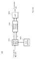
  • Fig.1(a) is a schematic illustration of coherent optical system model with modulating information over nonlinear spectrum.
  • a nonlinear optical transmission system 100 comprises a coherent transmitter 102, a coherent receiver 103 and an optical fiber 105.
  • the optical fiber 105 is preferably a nonlinear-dispersive fiber and may be implemented with single-mode fiber (SMF) or non-zero dispersion-shifted fiber (NZ-DSF) or other fiber types.
  • the coherent transmitter 102 as illustrated in Fig. 1(c) , comprises a digital-to-analog converter (DAC) 1021, an optical source 1023 and an electrical-to-optical converter 1022, e.g. a Mach-Zehnder IQ modulator.
  • DAC digital-to-analog converter
  • the nonlinear optical transmission system 100 further comprises a transmitter processor 101 and a receiver processor 104.
  • Information (or data) is firstly encoded through, for example, an encoder (not shown) and then sent to the transmitter processor 101 to generate a time-domain signal based on the encoded information.
  • the transmitter processor 101 is configured to generate at least one waveform in time domain q(t), e.g. soliton pulse(s), with an INFT algorithm such as Darboux Transform preferably.
  • information is encoded on nonlinear spectrum based on eigenvalue patterns ⁇ i 106 and a spectral modulation function 107 comprising discrete nonlinear spectrum Q d ( ⁇ i ).
  • the spectral modulation function 107 of each eigenvalue forms a QPSK constellation.
  • each 4 bits are mapped to a 2-soliton symbol of the constellation set.
  • each 2 bits are mapped to one of the spectral modulation function 107 and the corresponding soliton signal q(t) is then generated by the transmitter processor 101 with Darboux transform algorithm. Subsequently, the signal q(t) is sent to the coherent transmitter 102 for generating the corresponding optical signal to be transmitted.
  • the coherent receiver 103 After transmission over the optical fiber 105, the optical signal becomes distorted and the coherent receiver 103 detects the distorted signal.
  • the coherent receiver 103 as illustrated in Fig. 1(d) , comprises an optical local oscillator 1033 and an optical hybrid mixer 1031 together with optical-to-electrical converters 1032 which convert the optical signal into the corresponding electrical signal.
  • the converted distorted electrical signal in an analog form is sampled via an analog-to-digital converter (ADC) 1034 and processed by the receiver processor 104 that applies an NFT algorithm to recover both QPSK spectral phases of the distorted signal R(t).
  • ADC analog-to-digital converter
  • a nonlinear channel provided by the optical fiber 105 is equivalent to a linear channel in spectral domain and the information can be retrieved by applying linear filters/equalizers in the receiver processor 104.
  • Fig. 1(b) shows the equivalent linear channel model of the nonlinear optical transmission system 100 in Fig. 1(a) , indicating that the optical fiber 105 is equivalent to the linear channel 110 in spectral domain.
  • the transmitter processor 101 and the receiver processor 104 are placed outside the coherent transmitter 102 and the coherent receiver 103, it should be noted that they can be part of the coherent transmitter 108 and the coherent receiver 109, respectively, as illustrated in Fig. 1(b) .
  • Fig. 2 illustrates a method 200 comprising processing steps taken place in the transmitter processor 101 for generating a time-domain waveform with the INFT algorithm according to embodiments of the disclosure.
  • the INFT algorithm is configured to generate a multi-soliton waveform q(t) from discrete nonlinear spectrum pairs including spectral values and spectral modulation function, i.e. ( ⁇ i , Q d ( ⁇ i )), based on Darboux transform.
  • the method 200 further comprises a signal update step 205 and a spectral function update step 206.
  • the signal update step 205 updates the time-domain solitary waveform q(t) with spectral functions v k ( t ) which have been updated based on spectral values corresponding to eigenvalues ⁇ i at the spectral function update step 206.
  • at least one spectral function can be generated based on the at least one initial spectral function and the at least one spectral value at step 206 and the waveform can then be determined based on the at least one spectral function at step 205.
  • the signal update step 205 and the spectral function update step 206 are implemented recursively adding a new spectral value corresponding to ⁇ i to the current waveform.
  • the method 200 therefore comprises determining, at step 204, whether each of the N spectral values ⁇ i have been considered for the signal update step 205 and the spectral function update step 206. If each of the N spectral values ⁇ i have been considered, the INFT algorithm outputs a final waveform having the N desired spectral values at step 207 and ends at step 208. Otherwise, the INFT algorithm will repeat the signal update step 205 and the spectral function update step 206 until each of the N spectral values ⁇ i have been added to the time-domain solitary waveform q(t). It should be noted that the embodiment of Fig. 2 calculates the signal q ( t ) for every sample and the same procedure is also implemented for M signal samples at ( t 1 , t 2 , ..., t M ).
  • NFT Nonlinear Schrödiger
  • the inverse nonlinear Fourier transform maps the spectral components to the corresponding solution in time domain.
  • both pairs of ( ⁇ P ( t ; ⁇ ), ⁇ P ( t ; ⁇ *)) and ( ⁇ N ( t ; ⁇ ), ⁇ N ( t ; ⁇ * )) can be used as a basis for the solutions of (2) for ⁇ and are called canonical solutions.
  • the matrix S a ⁇ b * ⁇ * b ⁇ - a * ⁇ * is called the scattering matrix and it captures the required information to identify q(t). More precisely, at t ⁇ - ⁇ , where q(t) is absent, ⁇ N ( t ; ⁇ ) ⁇ e -j ⁇ t (1,0) T . For any finite t 0 , ⁇ N ( t 0 ; ⁇ ) captures the information of q ( t ), t ⁇ ( - ⁇ , t 0 ) by integrating over q ( t ) according to the temporal evolution. As a result, the signal q(t) can be uniquely described by knowing a ( ⁇ ) and b ( ⁇ ) for some particular ⁇ ⁇ C + .
  • the continuous spectrum corresponds to the dispersive part of signal q ( t ).
  • the discrete spectrum corresponds to the solitonic part of signal q(t).
  • b ⁇ lim t ⁇ + ⁇ e - j ⁇ t ⁇ 2 N
  • the signal q(t) can be characterized from Q c ( ⁇ ), ⁇ ⁇ R and the set of ( ⁇ i , Q d ( ⁇ i )) using an inverse nonlinear Fourier transform such as Riemann-Hilbert method.
  • an inverse nonlinear Fourier transform such as Riemann-Hilbert method.
  • the proposed algorithm based on the Darboux transformation is very useful when q(t) has only a discrete spectrum.
  • the discrete spectrum of q ⁇ ( t, z ) comprises the eigenvalues of q ( t , z ) and also ⁇ 0 (and ⁇ 0 * ),
  • the initial spectral conditions may include two parameters, e.g. a first initial parameter A i and a second initial parameter B i , where A i can be an arbitrary constant value.
  • a i can be an arbitrary constant value.
  • B i depends on eigenvalues ⁇ k and corresponding spectral amplitudes Q d ( ⁇ k ).
  • Fig. 3 illustrates a method 300 for implementing the initialization step 203 of method 200 according to embodiments of the disclosure.
  • i is set to be zero at step 302.
  • the method 300 comprises setting at least one initial spectral condition based on the at least one spectral modulation function for the corresponding spectral values at step 304.
  • the method 300 further comprises generating at least one initial spectral function v i ( t ), which comprises two components v i ,1 ( t ) and v i ,2 ( t ), for the corresponding spectral values based on the at least one initial spectral condition at step 305.
  • the first initial parameter A i can also be an arbitrary non-zero value except 1. Since there is one degree of freedom, if A i is set to some number, B i will result accordingly.
  • the step 304 and the step 305 are implemented recursively until each spectral values have been considered for setting the initial spectral conditions to the INFT algorithm.
  • Fig. 4 illustrates a method 400 for implementing the signal update step 205 of method 200 according to embodiments of the disclosure.
  • the method 400 determines the at least one waveform by recursively updating a current waveform based on a previously generated waveform, the at least one spectral function and the at least one spectral value.
  • the method 400 comprises updating, at step 402, the at least one waveform q(t) based on the at least one initial spectral function and continuing to update recursively the at least one waveform based on at least one updated spectral function until each spectral values have been considered.
  • the embodiment of Fig. 4 calculates the signal update of q ( t ) for every sample and the same procedure is also implemented for M signal samples at time instants ( t 1 , t 2 ,..., t M ).
  • Fig. 5 illustrates a method 500 for implementing the spectral function update step 206 of method 200 according to embodiments of the disclosure.
  • the method 500 generates the at least one spectral function by recursively updating a current spectral function based on the at least one spectral value and a previously generated spectral function.
  • the method 500 comprises updating, at step 504 and step 505, the at least one initial spectral function based on the at least one spectral value and continuing to update recursively at least one spectral function based on the at least one spectral value until each spectral values have been considered.
  • the method 500 therefore comprises determining, at step 503, whether each spectral value ⁇ i has been considered for the step 504 and the step 505. If all spectral values ⁇ i have been considered, the INFT algorithm outputs the updated spectral function v k ( t ) at step 506 to be used for the signal update step 205 and ends at step 507. Otherwise, the INFT algorithm will repeat the step 504 and the step 505 until all spectral values ⁇ i have been considered.
  • the embodiment of Fig. 5 calculates the updated spectral functions v k ( t ) for every sample and the same procedure is also implemented for M signal samples at ( t 1 , t 2 ,..., t M ).
  • v i ( v i ,1 , v i, 2 ) updates q(t) at step 205 or 400 and then this v i updates v k for k ⁇ i + 1 at step 500. Subsequently, the index i is increased and the signal update process 400 is continued.
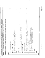
  • Algorithm 1 an example pseudo-code of the proposed INFT algorithm is shown in Algorithm 1 below (see also Fig. 10 ).
  • the pseudo-code computes the signal waveform q(t) for all spectral values (i.e. eigenvalues) ⁇ i at a time sample, which may be repeated for all time samples to generate the signal waveform q(t) at every sampling time t.
  • the pseudo-code can be simplified as shown in Algorithm 2 below (see also Fig. 11 ), resulting in a complexity to be further reduced by a factor of 2.
  • the proposed method can efficiently generate a multi-soliton waveform from the given discrete spectrum ( ⁇ i , Q d ( ⁇ i )).
  • solitary waveforms are generated for desired nonlinear spectrum.
  • the efficiency of the employed algorithms, e.g. Darboux transformation, for recursively generating an exact multi-soliton signal from the desired spectral amplitudes can be significantly improved through the proposed method.
  • Fig. 6 illustrates a method 600 comprising processing steps taken place in the receiver processor 104 for detecting at least one received waveform with NFT algorithm according to embodiments of the disclosure.
  • the NFT algorithm is configured to numerically compute the nonlinear spectrum of received pulses R ( t ) from samples thereof.
  • the method 600 comprises receiving the at least one waveform from the nonlinear channel at step 601.
  • the at least one received waveform comprises at least one spectral modulation function Q d ( ⁇ i ) of the nonlinear spectrum corresponding to at least one spectral value ⁇ i .
  • the at least one spectral modulation function comprises one or more spectral coefficients, e.g.
  • the method 600 comprises generating, at step 602, a plurality of samples of the at least one received waveform by sampling the at least one received waveform.
  • the method 600 further comprises dividing the plurality of samples of the at least one received waveform into a first sample portion and a second sample portion at step 603, computing a first spectral matrix in a forward sample direction during the first sample portion of the at least one received waveform at step 604, computing a second spectral matrix in a backward sample direction during the second sample portion of the at least one received waveform at step 605 and obtaining, at step 606, the at least one spectral modulation function for each of the at least one received waveform based on the first spectral matrix and the second spectral matrix.
  • the steps of dividing the plurality of samples of the at least one received waveform into the first sample portion and the second sample portion (603), computing the first spectral matrix in the forward sample direction (604) and the second spectral matrix in the backward sample direction (605) and obtaining the at least one spectral modulation function for the at least one received waveform (606) may be implemented for each eigenvalue/spectral value ⁇ i to calculate the corresponding spectral modulation function Q d ( ⁇ i ). Therefore, these steps may be repeatedly computed until each of the at least one spectral value ⁇ i has been considered.
  • Nonlinear Fourier transform is usually defined based on the Zakharov-Shabat system.
  • ⁇ ( t; ⁇ ) ( ⁇ 1 ( t; ⁇ ), ⁇ 2 ( t; ⁇ )) T
  • a ( ⁇ ) e + j ⁇ T 0 ⁇ 1 ( T 0 ; ⁇ )
  • b ( ⁇ ) e -j ⁇ T 0 ⁇ 2 ( T 0 ; ⁇ )
  • the discrete spectrum corresponds to the solitonic part of signal q(t).
  • the proposed method employing "forward-backward” algorithm is a general/universal method which can be applied to any integration based methods such as Crank-Nicolson algorithm to improve the numerical performance thereof. Using one of these methods, it numerically solves equation (9) partly in forward direction and partly in backward direction. Finally it combines the results to compute the nonlinear spectrum. With the same complexity, it has a much higher precision than the underlying method. Without loss of generality, this method is explained here for a particular underlying method which has a simple representation and estimates the spectrum with higher precision than the above mentioned algorithms. This underlying algorithm is called “Trapezoid Discretization" as it is based on trapezoid rule of integral.
  • the proposed method computes the nonlinear spectrum based on Trapezoid Discretization algorithm.
  • the trapezoid rule can be used to numerically compute ⁇ (T 0 ; ⁇ ).
  • the Trapezoid Discretization method shows the best accuracy compared to the other methods.
  • G n cos q n h sin q n h e j ⁇ n + j 2 ⁇ t n - sin q n h e - j ⁇ n - j 2 ⁇ t n cos q n h
  • G n ⁇ + j 2 t n sin q n h 0 e j ⁇ n + j 2 ⁇ t n e - j ⁇ n - j 2 ⁇ t n 0 .
  • w n + 1 ⁇ d d ⁇ w n + 1 , 1 , d d ⁇ w n + 1 , 2 T .
  • the final recursion looks like the layer-peeling algorithm. However, there are some small differences.
  • the layer-peeling algorithm is a kind of forward (Euler) algorithm and obtained from approximating q(t) as a piece-wise constant function.
  • the proposed algorithm is a kind of mid-point algorithms (Trapezoid rule) which usually provides better approximations (see Fig. 7 ).
  • the matrix F ( t ) can be approximated as a piece-wise constant function.
  • the other practical advantage is the equation has a much simpler form than the layer-peeling algorithm.
  • the first order approximation of G n gives the forward (Euler) discretization method.
  • h 1, cos(
  • h one has G n ⁇ 1 h q t n e j 2 ⁇ t n - h q * t n e - j 2 ⁇ t n 1 .
  • G n can be re-written as: G n ⁇ 1 1 + h 2 4 q n 2 1 - h 2 4 q n 2 h q t n e j 2 ⁇ t n - h q * t n e - j 2 ⁇ t n 1 - h 2 4 q n 2 , which is the normalized matrix of the Crank-Nicolson method for solving, i.e. ⁇ t n + 1 ⁇ - ⁇ t
  • the estimation error may exponentially grow with a slight change of step-size h.
  • a small numerical error in a ( ⁇ ) may lead to an exponentially large error in estimating b ( ⁇ ).
  • G n,kl denote the entry ( k, l ) of matrix G n .
  • the forward recursion computes ( L 11 , L 21 ) and its derivative, for 1 ⁇ n ⁇ m .
  • w n G n w n - 1
  • w 0 G 0 1 2 1
  • w n ⁇ G n w n - 1 ⁇ + G n ⁇ w n - 1
  • w 0 ⁇ G 0 1 2 ⁇ 1 0
  • the backward recursion computes (- R 12 , R 11 ) and its derivative, for m ⁇ n ⁇ N.
  • ⁇ n - 1 G n - 1 ⁇ n
  • ⁇ N ⁇ G N 1 2 ⁇ 0 1
  • G n - 1 is obtained by replacing h with -h in G n as follows:
  • the at least one received waveform comprises a 2-solitonic pulse.
  • This received pulse q(t) is symmetric and has only an imaginary component.
  • the proposed method further comprises truncating the pulse outside the interval t ⁇ [-5,5] in which contains more than 99.9% of pulse energy.
  • the truncated pulse is uniformly sampled by N samples to be supplied to the proposed forward-backward algorithm (FB).
  • the first spectral matrix and the second spectral matrix are computed based on the Trapezoid Discretization (TD) method. It should be noted that the first spectral matrix and the second spectral matrix may also be computed based on other numerical NFT algorithms such as Crank-Nicolson algorithm (CN) and Ablowitz-Ladik discretization algorithm (AL).
  • Table 1 shows the discrete spectral amplitudes (i.e. the spectral modulation function) Q d ( ⁇ i ) and the corresponding spectral coefficients a ( ⁇ ) computed by applying different algorithms in terms of N.
  • the sample portion dividing ratio c can also be any arbitrary value, or be chosen based on equation (21).
  • the results are compared for the different algorithms: AL, CN, TD and FB, where FB combines the proposed forward-backward algorithm with the Trapezoid Discretization method whereas AL, CN and TD merely apply their corresponding integration based methods alone (i.e.
  • Fig. 8(b) shows the results of ⁇ 1 ( t ; ⁇ )
  • Fig. 8(c) shows the results of ⁇ 2 ( t ; ⁇ )
  • N 10 6
  • the proposed method employing the forward-backward algorithm provides an efficient way to compute the nonlinear spectrum of pulses with finite pulse width.
  • the proposed "forward-backward method” is more accurate and more robust than other discretization algorithms.
  • it can be implemented in parallel which increases computation speed by a factor of 2 and the total computational complexity of the proposed method is O ( N ) per eigenvalue.
  • a more stable and numerically more precise algorithm is provided to an optical transmitter and an optical receiver of a nonlinear optical transmission system, in order to efficiently generate and detect solitary waveforms for desired nonlinear spectrum with improved accuracy.
  • the proposed method enhances the efficiency for the INFT, which can be implemented, for example, in the future Nonlinear Frequency Division Multiplexing (NFDM) schemes which improve the signal-to-noise ratio (SNR) and/or spectral efficiency performance of optical transport systems while keeping the very-large-scale integration (VLSI) complexity low.
  • NFDM Nonlinear Frequency Division Multiplexing
  • SNR signal-to-noise ratio
  • VLSI very-large-scale integration
  • the proposed method has lower complexity than the other algorithms to generate a waveform with desired nonlinear spectrum.
  • the proposed method has higher stability and higher accuracy in numerically computing the nonlinear spectrum from samples of a waveform than other discretization algorithms, especially when the sampling rate is low, showing an advantage of parallel implementation in hardware which can reduce the computation time.
  • the proposed method is a good candidate for the future NFDM optical systems as it is simple, robust and sufficiently precise for NFT implementation.
  • any block diagrams herein represent conceptual views of illustrative circuitry embodying the principles of the invention.
  • any flow charts, flow diagrams, state transition diagrams, pseudo code, and the like represent various processes which may be substantially represented in computer readable medium and so executed by a computer or processor, whether or not such computer or processor is explicitly shown.
  • processor or “computer” should not be construed to refer exclusively to hardware capable of executing software, and may implicitly include, without limitation, digital signal processor (DSP) hardware, network processor, application specific integrated circuit (ASIC), field programmable gate array (FPGA), read-only memory (ROM) for storing software, random-access memory (RAM), and non-volatile storage.
  • DSP digital signal processor
  • ASIC application specific integrated circuit
  • FPGA field programmable gate array
  • ROM read-only memory
  • RAM random-access memory
  • non-volatile storage Other hardware, conventional and/or custom, may also be included.

Landscapes

  • Physics & Mathematics (AREA)
  • Engineering & Computer Science (AREA)
  • Computer Networks & Wireless Communication (AREA)
  • Signal Processing (AREA)
  • Electromagnetism (AREA)
  • Discrete Mathematics (AREA)
  • General Physics & Mathematics (AREA)
  • Mathematical Physics (AREA)
  • Optical Communication System (AREA)

Abstract

This application relates to a method for generating a waveform in an optical transmission system having a nonlinear channel, wherein the waveform is generated based on at least one spectral modulation function depending on at least one spectral value. The method comprises: receiving the at least one spectral modulation function and the at least one corresponding spectral value, setting an initial spectral condition based on the at least one spectral modulation function, generating at least one initial spectral function based on the initial spectral condition and the at least one spectral value, generating at least one spectral function based on the at least one initial spectral function and the at least one spectral value and determining the at least one waveform based on the at least one spectral function. This application also relates to a method for detecting a waveform having a nonlinear spectrum received via a nonlinear channel, the method comprises receiving the waveform from the nonlinear channel, wherein the received waveform has associated at least one spectral modulation function of the nonlinear spectrum depending on at least one spectral value, generating, by sampling the waveform, a plurality of samples of the waveform, dividing the plurality of samples into a first sample portion and a second sample portion, computing a first spectral matrix in a forward sample direction for the first sample portion, computing a second spectral matrix in a backward sample direction for the second sample portion, and obtaining, based on the first spectral matrix and the second spectral matrix, the at least one spectral modulation function for the received waveform.

Description

    Technical Field
  • This application relates to transmitters and receivers for optical transmission systems using a nonlinear channel, particularly for modulation over nonlinear spectrum including nonlinear frequency division multiplexing (NFDM).
  • Background
  • It is well-known that Nonlinear Schrödinger equation (NLSE) characterizes the interplay between dispersion and Kerr nonlinearity in the transmission channel and that NLSE can be therefore used to model signal propagation in an optical fiber. To study how the optical fields propagate in an optical fiber according to NLSE, a suitable method called nonlinear Fourier transform (NFT) has been applied, which describes the optical fields by a nonlinear spectrum and results in a simple linear channel transfer function even for strongly nonlinear propagation along a fiber link. In particular, general principles for modulation over nonlinear spectrum including nonlinear frequency division multiplexing (NFDM) have been investigated and current promising experiments show a high potential of "Nonlinear Frequency Division Multiplexing (NFDM)" schemes to be the future of long-haul fiber optical transmission. In principle, a nonlinear-dispersive fiber is a favorable "linear" channel in nonlinear spectral domain. In an NFDM scheme, the information is modulated over nonlinear spectrum and is transformed to a waveform in time domain via Inverse Nonlinear Fourier Transform (INFT). The waveforms which are transformed nonlinearly in time domain have linear transformations in nonlinear Fourier spectrum. Therefore, the changes of waveforms can be easily tracked in nonlinear spectral domain, i.e. the distortion of the waveforms caused by both fiber nonlinearity and dispersion can be easily analyzed and compensated in spectral domain, which motivates to first modulate information in nonlinear spectrum and then to map, via INFT, the nonlinear spectrum to the corresponding optical fields in time domain. The optical fields are subsequently propagating in an optical fiber causing waveform distortion of the optical fields. The nonlinearly distorted waveforms can be successfully detected by a Nonlinear Fourier Transform (NFT) algorithm at a receiver from corresponding nonlinear spectrum. In the receiver, the information can be retrieved from the nonlinear spectrum of the received optical fields computed by NFT. The main reason of modulating information in nonlinear spectrum is that the equivalent channel in nonlinear spectral domain is linear and the information can be retrieved by applying linear filters/equalizers.
  • The nonlinear spectrum can be divided into two parts: the continuous spectrum, corresponding to the "dispersive" signal components, and the discrete spectrum, corresponding to the "solitonic" (non-dispersive) signal components. The discrete spectrum is characterized by (λi , Qd (λi )) where λi is an isolated "nonlinear frequency" in upper complex plane, i.e. the eigenvalue of Lax operator, and Qd (λi ) is the discrete spectral modulation function at λi , i.e. the spectral amplitude at this eigenvalue. In general, INFT can be computed by solving a Riemann-Hilbert system of algebraic equations. However, the computational complexity of the method grows cubic in terms of the number of eigenvalues of discrete spectrum. For instance, if the discrete nonlinear spectrum comprises N pairs: (λi , Qd (λi )), i.e. there are N non-zero eigenvalues (in the positive complex plane), one needs to inverse a matrix of size N for each signal sample. Therefore, the complexity scales O(N 2.80) per sample. Alternatively, Darboux transform (DT) which has the complexity O(N 2) can be used. In the currently known method based on Darboux transform, a multi-soliton signal can be generated from given eigenvalues λi but it is not known how to design a signal if the desired spectral amplitudes Qd (λi ) shall also be included. In particular, the method needs additional 2N initial parameters which determine the spectral amplitudes. It is not yet known how to choose these initial parameters for the desired spectral amplitudes.
  • Furthermore, the nonlinear Fourier transform is usually defined based on the Zakharov-Shabat system. Considering a pulse q(t) with a finite pulse width, in practice, the pulse q(t) can be represented by N samples. At the receiver, the nonlinear spectrum can be numerically computed by numerical methods such as Forward discretization, Crank-Nicolson method, Layer-peeling method and Ablowitz-Ladick discretization. However, most of these methods converge slowly and show unacceptable numerical error in estimating discrete spectra when N is not very large. A better estimation like Layer-peeling algorithm usually results in higher computational complexity.
  • Accordingly, there is a need for a nonlinear optical transmission system to efficiently generate and detect solitary waveforms for desired nonlinear spectrum with improved accuracy. In order to solve the aforementioned problems, the present application proposes a more stable and numerically more precise algorithm to be used in an optical transmitter and an optical receiver of a nonlinear optical transmission system.
  • Summary
  • In view of this need, the present document proposes methods and devices having the features of the respective independent claims for generating at least one waveform in an optical transmission system having a nonlinear-dispersive channel, where the at least one waveform is generated based on at least one spectral modulation function, each spectral modulation function depending on a spectral value, and for detecting at least one waveform having a nonlinear spectrum received via the nonlinear-dispersive channel in the optical transmission system.
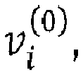
  • An aspect of the disclosure relates to a waveform generating method. The method may comprise receiving the at least one spectral modulation function and the at least one corresponding spectral value. Data may be encoded onto the at least one spectral modulation function. The at least one spectral modulation function may comprise, for example, spectral amplitudes Qd (λi ) of a discrete nonlinear spectrum of the waveform. The method may comprise setting at least one initial spectral condition, e.g. Bi , based on the at least one spectral modulation function and the at least one spectral value, e.g. λi . The method may comprise generating at least one initial spectral function based on the at least one initial spectral condition. In an embodiment, the at least one initial spectral function may be a vector function, e.g. v i 0 ,
    Figure imgb0001
    or a scalar function, e.g. ρ i 0 .
    Figure imgb0002
    In particular, the at least one initial spectral condition may comprise, for example, a first initial parameter, e.g. Ai, and a second initial parameter, e.g. Bi ,. Preferably, the first initial parameter may comprise a constant value ci . Furthermore, the second initial parameter may be proportional to the at least one spectral modulation function. For example, the second initial parameter may be set or computed based on a formula of B i = - c i Q d λ i λ i - λ i * k = 1 , k i N λ i - λ k λ i - λ k * .
    Figure imgb0003
  • The method may further comprise generating at least one spectral function based on the at least one initial spectral function v i 0 t
    Figure imgb0004
    or ρ i 0 t
    Figure imgb0005
    and the at least one spectral value λi. For example, the at least one initial spectral function may be update based on the at least one spectral value. The method may further comprise determining the waveform based on the at least one spectral function. For example, the at least one waveform may be determined based on the at least one initial spectral function.
  • According to the disclosure, generating the at least one spectral function may comprise recursively updating a current spectral function based on the at least one spectral value and a previously generated spectral function. For example, the at least one spectral function may be obtained in response to updating the at least one initial spectral function and the at least one spectral function may be updated recursively based on the at least one spectral value. In an embodiment, the at least one spectral function may be a vector function, e.g. v k i t ,
    Figure imgb0006
    or a scalar function, e.g. ρ k i t .
    Figure imgb0007
    Furthermore, determining the waveform may comprise recursively updating a current waveform based on a previously generated waveform, the at least one spectral function and the at least one spectral value. For example, the at least one waveform may be recursively updated based on the at least one updated spectral function. In embodiments, the at least one spectral function may be updated recursively until each of a plurality of spectral values has been considered. Moreover, the at least one waveform may be updated recursively until each of the spectral values has been considered. In a preferred embodiment, the step of updating the at least one spectral function or the at least one waveform may be based on Darboux transform.
  • According to the disclosure, the at least one spectral modulation function may comprise a discrete nonlinear spectrum of the at least one waveform. The discrete nonlinear spectrum may be encoded with data and may be given or predetermined according to a desired nonlinear spectrum. In embodiments, the at least one waveform may comprise a solitary waveform, e.g. a multi-soliton waveform. The at least one waveform may comprise a plurality of samples. The method may further comprise updating recursively the at least one waveform for the plurality of samples.
  • Configured as above, by setting appropriate initial spectral conditions, based on the at least one spectral modulation function, and generating at least one initial spectral function, based on the at least one initial spectral condition, the at least one waveform can be efficiently generated from the at least one spectral modulation function, i.e. the desired nonlinear discrete spectrum, thereby reducing the computational complexity for INFT.
  • Another aspect of the disclosure relates to a waveform detecting method. The method may comprise receiving the at least one waveform from the nonlinear channel. In particular, the at least one received waveform may have associated at least one spectral modulation function of the nonlinear spectrum depending on at least one spectral value. The method may comprise generating a plurality of samples of the at least one received waveform by sampling the at least one received waveform. In embodiments, the at least one received waveform may have a finite pulse width. In such embodiments, the method may further comprise truncating the at least one received waveform.
  • The method may further comprise dividing the plurality of samples of the at least one received waveform into a first sample portion and a second sample portion. In an embodiment, the first sample portion and the second sample portion may comprise a same number of samples. That is, the duration of the first sample portion may be equal to the duration of the second sample portion, which may correspond to one half of the pulse width of the at least one received waveform. However, other partitions of the waveform samples are possible. In another embodiment, dividing the plurality of samples of the received waveform into the first sample portion and the second sample portion may be based on a sample portion dividing ratio c. The sample portion dividing ratio c may be any arbitrary value between 0 and 1. Preferably, the sample portion dividing ratio may be chosen based on formula: c = arg min t = T 0 2 c - 1 q t exp 2 η t .
    Figure imgb0008
    where T 0 represents the one half of the pulse width of the received waveform and η represents the imaginary part of the at least one spectral value.
  • According to the disclosure, the method may further comprise computing a first spectral matrix in a forward sample direction, during the first sample portion of the at least one received waveform, and computing a second spectral matrix in a backward sample direction, during the second sample portion of the at least one received waveform. In a preferred embodiment, the first spectral matrix and the second spectral matrix may be computed based on Trapezoid Discretization method. In other embodiments, the computation of the first spectral matrix and the second spectral matrix may also be based on any integration based methods such as Crank-Nicolson algorithm or Ablowitz-Ladik discretization algorithm. Furthermore, the method may comprise obtaining the at least one spectral modulation function for the at least one received waveform based on the first spectral matrix and the second spectral matrix. In embodiments, the at least one received waveform may comprise a 2-solitonic pulse and the at least one spectral modulation function may comprise one or more spectral coefficients. In other words, the at least one spectral modulation function may be computed based on one or more spectral coefficients.
  • Furthermore, the steps of dividing the plurality of samples of the at least one received waveform into the first sample portion and the second sample portion, computing the first spectral matrix in the forward sample direction and the second spectral matrix in the backward sample direction and obtaining the at least one spectral modulation function for the at least one received waveform may be implemented for each spectral value, e.g. λi , to calculate/compute the corresponding spectral modulation function, e.g. Qd (λi ). Accordingly, these aforementioned steps may be repeated until each spectral value has been considered.
  • Configured as above, by computing the nonlinear spectrum partly in forward direction and partly in backward direction, the numerical estimation of the nonlinear spectrum is improved, providing a more stable and more precise algorithm for NFT especially in case of low sampling rate. In other words, the proposed method enables a simple, robust and sufficiently precise NFT, thereby advantageously reducing computational time to allow parallel implementation in hardware, which is a potential candidate for the future NFDM optical systems. Another aspect of the disclosure relates to a transmitter. The transmitter may be configured to generate at least one waveform for transmission via a nonlinear channel. In particular, the at least one waveform may be generated based on at least one spectral modulation function depending on at least one spectral value. The transmitter may comprise an encoder and a processor. The encoder may be configured to encode data onto the at least one spectral modulation function. The processor may be coupled with the encoder and may be configured to receive the at least one spectral modulation function encoded with the data from the encoder and the at least one corresponding spectral value. The processor may be configured to set at least one initial spectral condition, for example, Bi , based on the at least one spectral modulation function, e.g. Qd (λi ), and the at least one spectral value, e.g. λi . In particular, the at least one initial spectral condition may comprise, for example, a first initial parameter, e.g. Ai , and a second initial parameter, e.g. Bi ,. Preferably, the first initial parameter may comprise a constant value ci . Furthermore, the second initial parameter may be proportional to the at least one spectral modulation function. For example, the second initial parameter may be set or computed based on a formula B i = - c i Q d λ i λ i - λ i * k = 1 , k i N λ i - λ k λ i - λ k * .
    Figure imgb0009
  • According to the disclosure, the processor may be further configured to generate at least one initial spectral function based on the at least one initial spectral condition. In an embodiment, the at least one initial spectral function may be a vector function, e.g. v i 0 ,
    Figure imgb0010
    or a scalar function, e.g. ρ i 0 .
    Figure imgb0011
    Furthermore, the processor may be configured to generate at least one spectral function based on the at least one initial spectral function and the at least one spectral value. For example, the at least one initial spectral function may be updated based on the at least one spectral value. The processor may be configured to further determine the waveform based on the at least one spectral function. For example, the at least one waveform may be determined based on the at least one initial spectral function. In an embodiment, the at least one spectral function may be a vector function, e.g. v k i t ,
    Figure imgb0012
    or a scalar function, e.g. ρ k i t .
    Figure imgb0013
  • The determined waveform(s) may then be transmitted via the nonlinear channel to a receiver to convey information in an optical transmission system.
  • Another aspect of the disclosure relates to a receiver. The receiver may be configured to detect at least one waveform having a nonlinear spectrum received via a nonlinear channel in an optical transmission system. In particular, the at least one received waveform may have associated at least one spectral modulation function of the nonlinear spectrum depending on at least one spectral value. The receiver may comprise a processor. The processor may be configured to generate a plurality of samples of the at least one received waveform by sampling the at least one received waveform. The processor may be configured to divide the plurality of samples of the at least one received waveform into a first sample portion and a second sample portion. In embodiments, the plurality of samples of the received waveform may be divided into the first sample portion and the second sample portion based on a sample portion dividing ratio c. In one embodiment, the sample portion dividing ratio c may be any arbitrary value between 0 and 1. In another embodiment, the sample portion dividing ratio may be chosen based on formula: c = arg min t = T 0 2 c - 1 q t exp 2 η t .
    Figure imgb0014
    where T 0 represents the one half of the pulse width of the received waveform and η represents the imaginary part of the at least one spectral value.
  • According to the disclosure, the processor may be further configured to compute a first spectral matrix in a forward sample direction during the first sample portion of the at least one received waveform and compute a second spectral matrix in a backward sample direction during the second sample portion of the at least one received waveform. Furthermore, the processor may be configured to obtain the at least one spectral modulation function for the at least one received waveform based on the first spectral matrix and the second spectral matrix.
  • Furthermore, dividing the plurality of samples of the at least one received waveform into the first sample portion and the second sample portion, computing the first spectral matrix in the forward sample direction and the second spectral matrix in the backward sample direction and obtaining the at least one spectral modulation function for the at least one received waveform may be implemented for each of the at least one spectral value, e.g. λi , to calculate/compute the corresponding spectral modulation function, e.g. Qd (λi ), and may accordingly be repeated until each of the at least one spectral value has been considered.
  • The receiver may further comprise a decoder to decode data from the obtained at least one spectral modulation function (Qd (λi )) for the received waveform (R(t)), thereby determining the information transmitted via the nonlinear channel.
  • Configured as above, the proposed transmitter and receiver are implemented with more stable and numerically more precise algorithms to efficiently generate and detect, with improved accuracy, solitary waveforms according to desired nonlinear spectrum for nonlinear optical transmission. In other words, the INFT and NFT computations become more efficient by using the proposed devices, thereby reducing the complexity of hardware implementations. Furthermore, improved robustness of the proposed devices is suitable for the future NFDM optical systems.
  • It will be appreciated that method steps and device features may be interchanged in many ways. In particular, the details of the disclosed device can be implemented as a method, as the skilled person will appreciate.
  • Brief Description of the Figures
  • Embodiments of the disclosure are explained below in an exemplary manner with reference to the accompanying drawings, wherein
    • Fig.1(a) schematically illustrates a coherent optical system model with modulating information over nonlinear spectrum;
    • Fig.1(b) schematically illustrates an equivalent linear channel model of a nonlinear optical transmission system of Fig. 1(a);
    • Fig. 1(c) schematically illustrates an example of a coherent transmitter used in the nonlinear optical transmission system of Fig. 1(a);
    • Fig. 1(d) schematically illustrates an example of a coherent receiver used in the nonlinear optical transmission system of Fig. 1(a);
    • Fig. 2 illustrates an example of the proposed method for generating time-domain waveform with INFT algorithm according to embodiments of the disclosure;
    • Fig. 3 illustrates an example of the proposed method for implementing the initialization step 203 of Fig. 2 according to embodiments of the disclosure;
    • Fig. 4 illustrates an example of the proposed method for implementing the signal update step 205 of Fig. 2 according to embodiments;
    • Fig. 5 illustrates an example of the proposed method for implementing the spectral function update step 206 of Fig. 2 according to embodiments;
    • Fig. 6 illustrates an example of the proposed method for detecting at least one received waveform with NFT algorithm according to embodiments;
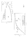
    • Fig. 7(a) illustrates a comparison of the precision for numerical solutions with respect to x(t) = exp(t 2/2) using different numerical methods;
    • Fig. 7(b) illustrates a comparison of the precision for numerical solutions with respect to x(t) = exp(∫ sech(t)dt) using different numerical methods;
    • Fig. 8(a) illustrates absolute value of samples of a 2-solitonic pulse q(tn ) received via a nonlinear channel in an optical transmission system of Fig. 1(a) according to embodiments;
    • Fig. 8(b)-(d) illustrates a comparison of the precision for numerical estimation of ψ(tn ;λ) using FB and AL discretization algorithm according to embodiments;
    • Fig. 9 shows Table 1 indicating discrete spectral amplitudes Qd (λi ) and corresponding spectral coefficients a(λ) computed by different algorithms;
    • Fig. 10 shows a first example algorithm for computing the inverse nonlinear Fourier transform based on the Darboux transform; and
    • Fig. 11 shows a second example algorithm for computing the inverse nonlinear Fourier transform based on the Darboux transform.
    Detailed Description
  • This disclosure comprises providing an optical transmitter and an optical receiver of a nonlinear optical transmission system with a more stable and numerically more precise algorithm to efficiently generate and detect solitary waveforms for desired nonlinear spectrum with improved accuracy.
  • The nonlinear optical transmission system may be based on the system architecture proposed in the documents "V. Aref et.al., 'Experimental Demonstration of Nonlinear Frequency Division Multiplexed Transmission,' ECOC 2015", and "H. Bülow, 'Experimental Demonstration of Optical Signal Detection Using Nonlinear Fourier Transform,' JLT, vol. 33, no. 7, 2015" which are incorporated herein by reference in their entirety.
  • Fig.1(a) is a schematic illustration of coherent optical system model with modulating information over nonlinear spectrum. A nonlinear optical transmission system 100 comprises a coherent transmitter 102, a coherent receiver 103 and an optical fiber 105. The optical fiber 105 is preferably a nonlinear-dispersive fiber and may be implemented with single-mode fiber (SMF) or non-zero dispersion-shifted fiber (NZ-DSF) or other fiber types. The coherent transmitter 102, as illustrated in Fig. 1(c), comprises a digital-to-analog converter (DAC) 1021, an optical source 1023 and an electrical-to-optical converter 1022, e.g. a Mach-Zehnder IQ modulator. The nonlinear optical transmission system 100 further comprises a transmitter processor 101 and a receiver processor 104. Information (or data) is firstly encoded through, for example, an encoder (not shown) and then sent to the transmitter processor 101 to generate a time-domain signal based on the encoded information. The transmitter processor 101 is configured to generate at least one waveform in time domain q(t), e.g. soliton pulse(s), with an INFT algorithm such as Darboux Transform preferably. To achieve NFDM transmission in the nonlinear optical transmission system 100, information is encoded on nonlinear spectrum based on eigenvalue patterns λi 106 and a spectral modulation function 107 comprising discrete nonlinear spectrum Qd (λi ). In one example, NFDM transmission is demonstrated based on modulation of discrete spectrum by generating a constellation set from multiplexing two eigenvalues, λ 1 = 0.5j and λ 2= 1j, where j = - 1 ,
    Figure imgb0015
    according to the eigenvalue patterns 106. The spectral modulation function 107 of each eigenvalue forms a QPSK constellation. In the example, each 4 bits are mapped to a 2-soliton symbol of the constellation set. In particular, each 2 bits are mapped to one of the spectral modulation function 107 and the corresponding soliton signal q(t) is then generated by the transmitter processor 101 with Darboux transform algorithm. Subsequently, the signal q(t) is sent to the coherent transmitter 102 for generating the corresponding optical signal to be transmitted.
  • After transmission over the optical fiber 105, the optical signal becomes distorted and the coherent receiver 103 detects the distorted signal. It should be understood that the coherent receiver 103, as illustrated in Fig. 1(d), comprises an optical local oscillator 1033 and an optical hybrid mixer 1031 together with optical-to-electrical converters 1032 which convert the optical signal into the corresponding electrical signal. The converted distorted electrical signal in an analog form is sampled via an analog-to-digital converter (ADC) 1034 and processed by the receiver processor 104 that applies an NFT algorithm to recover both QPSK spectral phases of the distorted signal R(t). Since information is modulated in nonlinear spectrum, a nonlinear channel provided by the optical fiber 105 is equivalent to a linear channel in spectral domain and the information can be retrieved by applying linear filters/equalizers in the receiver processor 104. Fig. 1(b) shows the equivalent linear channel model of the nonlinear optical transmission system 100 in Fig. 1(a) , indicating that the optical fiber 105 is equivalent to the linear channel 110 in spectral domain. Although it is shown in Fig. 1(a) that the transmitter processor 101 and the receiver processor 104 are placed outside the coherent transmitter 102 and the coherent receiver 103, it should be noted that they can be part of the coherent transmitter 108 and the coherent receiver 109, respectively, as illustrated in Fig. 1(b) .
  • Fig. 2 illustrates a method 200 comprising processing steps taken place in the transmitter processor 101 for generating a time-domain waveform with the INFT algorithm according to embodiments of the disclosure. In the embodiments, the INFT algorithm is configured to generate a multi-soliton waveform q(t) from discrete nonlinear spectrum pairs including spectral values and spectral modulation function, i.e. (λi ,Qd (λi )), based on Darboux transform. After starting the INFT algorithm at step 201, the method 200 comprises receiving at least one spectral modulation function and at least one corresponding spectral value at step 202 where N discrete spectrum pairs (λi, Qd (λi )), i = 1, ..., N, and M signal samples at (t1 , t 2,..., tM ) are given, followed by an initialization step 203 which sets initial spectral conditions for the INFT algorithm (i = 0). The method 200 further comprises a signal update step 205 and a spectral function update step 206. The signal update step 205 updates the time-domain solitary waveform q(t) with spectral functions vk (t) which have been updated based on spectral values corresponding to eigenvalues λi at the spectral function update step 206. In other words, at least one spectral function can be generated based on the at least one initial spectral function and the at least one spectral value at step 206 and the waveform can then be determined based on the at least one spectral function at step 205. In particular, the signal update step 205 and the spectral function update step 206 are implemented recursively adding a new spectral value corresponding to λi to the current waveform. The method 200 therefore comprises determining, at step 204, whether each of the N spectral values λi have been considered for the signal update step 205 and the spectral function update step 206. If each of the N spectral values λi have been considered, the INFT algorithm outputs a final waveform having the N desired spectral values at step 207 and ends at step 208. Otherwise, the INFT algorithm will repeat the signal update step 205 and the spectral function update step 206 until each of the N spectral values λi have been added to the time-domain solitary waveform q(t). It should be noted that the embodiment of Fig. 2 calculates the signal q(t) for every sample and the same procedure is also implemented for M signal samples at (t 1, t 2, ..., tM ).
  • In the following, the principle of the proposed method generating the desirable solitary waveform is explained. Considering the Nonlinear Schrödiger (NLS) equation, z q t z - 2 t 2 q t z = 2 q t z 2 q t z .
    Figure imgb0016
    where z is the transmission distance. Nonlinear Fourier Transform (NFT) (or inverse scattering method) is an efficient way to solve this nonlinear differential equation or track the evolution of its solutions. NFT is a bijective mapping of a solution from time domain into a different domain, e.g. frequency/spectral domain, called nonlinear spectrum. The spectral components transform in z linearly. The inverse nonlinear Fourier transform (INFT) maps the spectral components to the corresponding solution in time domain. One can use Zakharov-Shabat system to characterize the nonlinear spectrum. The NLS equation is the compatibility condition of the following two linear equations: t v t z q λ = - q t z - q * t z v t z q λ ,
    Figure imgb0017
    z v t z q λ = 2 2 - j q t z 2 - 2 λq t z - jq t t z 2 λ q * t z - j q t * t z - 2 2 + j q 2 v t z q λ ,
    Figure imgb0018
    where λ is the spectral parameter, v(t,z; q,λ) is a 2 × 1 vector, qt denotes ∂q/∂t and q* denotes complex conjugate of q. It is understood that j = - 1
    Figure imgb0019
    for representing complex numbers. By differentiating (2) and (3) with respect to z and t, the right sides become equal if q(t,z) satisfies the NLS equation (1) . In particular, this implies that the nonlinear Schrödinger equation possess a "hidden linearity" in the form of (2) and (3). The temporal linear operator (2) and the spatial linear operator (3) are called the Lax pair of (1).
  • Assuming that |q(t,z)| vanishes sufficiently fast as |t| → ∞, or z → ∞, then, the following result is obtained: t v t z q λ t - 0 0 v t z q λ .
    Figure imgb0020
  • It is implied that v t z q λ t c 1 e - jλt , c 2 e + jλt T
    Figure imgb0021
    for some constants c 1, c 2C, i.e. a set of complex numbers. Similarly, v t z q λ z z 1 e + 2 z , z 2 e - 2 z T .
    Figure imgb0022
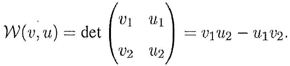
    Focusing on the temporal equation and reviewing some results, for presentation simplicity, dependency on z is omitted. Considering v(t;λ) as the elements of the vector space V equipped with the Wronskian product, W v u = det v 1 u 1 v 2 u 2 = v 1 u 2 - v 1 v 2 .
    Figure imgb0023
    the adjoint of any vector v(t) ∈ V is defined as v t = v 2 * - v 1 * .
    Figure imgb0024
  • Here, the following properties are shown:
    • u(t; µ) = v(t; λ = µ*) is a solution of (2) for λ = µ if v(t; µ*) is its solution for λ = µ*.
    • Let v(t;λ) be a solution of (2). W( v, v) = |v 1|2 + |v 2|2 = c for some constant cR independent of t.
    • If W( v ,v) ≠ 0, then v (t;λ*) and v(t;λ) are linearly independent and hence, they form a basis for the solution subspace of λ.
  • Some initial conditions are required for determining a specific temporal solution. Assuming λC +, i.e. the eigenvalues are located on the upper complex plane, and defining φP (t;λ), φ P (t;λ*), φN (t;λ) and φ N (t;λ*) with the following boundary conditions: ϕ P t λ t 0 1 e jλt , ϕ N t λ t 1 0 e - jλt
    Figure imgb0025
    ϕ P t λ * t 1 0 e - jλt , ϕ N t λ * t 0 - 1 e jλt
    Figure imgb0026
    one can see that W(φP (t;λ), φ P (t;λ*)) = -1 and W(φN (t;λ), φ N (t;λ*)) = -1. Therefore, both pairs of (φP (t;λ), φ P (t;λ*)) and (φN (t;λ), φ N (t;λ*)) can be used as a basis for the solutions of (2) for λ and are called canonical solutions. Thus, ϕ N t λ , ϕ N t λ * = ϕ P t λ * , ϕ P t λ a λ b * λ * b λ - a * λ * ,
    Figure imgb0027
    where a(λ) = W(φN (t;λ),φP (t;λ)) and b(λ) = W( φ P (t;λ*),φN (t;λ)). Note that a(λ) and b(λ) are independent of t. The matrix S = a λ b * λ * b λ - a * λ *
    Figure imgb0028
    is called the scattering matrix and it captures the required information to identify q(t). More precisely, at t → -∞, where q(t) is absent, φN (t;λ) → e-jλt (1,0) T. For any finite t 0, φN (t 0;λ) captures the information of q(t), t ∈ (-∞, t 0) by integrating over q(t) according to the temporal evolution. As a result, the signal q(t) can be uniquely described by knowing a(λ) and b(λ) for some particular λC +.
  • If q(t) decays faster than any polynomial, it is shown that φN (t;λ)e +jλt and φP (t;λ)e-jλt are analytic in upper-half complex plane and consequently, a(λ) = W(φN (t;λ),φP (t;λ)) is analytic in the same domain. It implies that the zeros of a(λ) are isolated. It is noted that φP (t;λ)e +jλt is only analytic in lower-half complex plane and therefore, b(λ) is not analytic in general.
  • Moreover, the projection (4) is well-defined for λR as the canonical solutions are bounded. It has been explained that solutions for λ* can be constructed from the solutions for λ. Therefore, one needs to focus on upper or lower half of complex plane. For λC +, φN (t;λ) and φ P (t;λ*) are unbounded as t → +∞. However, the projection (4) is still well-defined when a(λ) = 0. These λ (and λ*) are the eigenvalues of the corresponding spectral operator: j t - q t z - q * t z - t v = λv .
    Figure imgb0029
  • This can be immediately derived from reordering the temporal equation (2). The Zakharov-Shabat system has two types of spectrum: the discrete spectrum and the continuous spectrum. The latter is defined as: Q c λ = b λ a λ
    Figure imgb0030
    for λR. The continuous spectrum corresponds to the dispersive part of signal q(t). The discrete spectrum is defined over zeros of a(λ): Q d λ i = b λ i λ i ,
    Figure imgb0031
    where a'(λi ) = λ a λ | λ = λ i
    Figure imgb0032
    for all {λ 1,···,λn } ⊂ C + \R with the finite set satisfying a(λ) = 0.
  • The discrete spectrum corresponds to the solitonic part of signal q(t). Here, the spectral coefficients a(λ) and b(λ) are given by a λ = lim t + e + jλt ϕ 1 N , b λ = lim t + e - jλt ϕ 2 N
    Figure imgb0033
  • The signal q(t) can be characterized from Qc (λ), λR and the set of (λi ,Qd (λi )) using an inverse nonlinear Fourier transform such as Riemann-Hilbert method. On the other hand, the proposed algorithm based on the Darboux transformation is very useful when q(t) has only a discrete spectrum.
  • The Darboux transform (DT) was first introduced in the context of Sturm-Liouville differential equations. Later, it was extended to nonlinear integrable systems, providing the possibility to construct from one solution of an integrable equation another solution. The proposed algorithm works based on the following theorem.
  • Theorem: Considering an absolutely integrable q(t,z) with the scattering functions a(λ) and b(λ) at z = 0 and assuming that the nontrivial (ψ 1(t,z),ψ 2(t,z)) T fulfills (2) and (3) for some λ 0 such that λ 0 - λ 0 * > 0
    Figure imgb0034
    and a(λ 0) ≠ 0 (it is not an eigenvalue), i.e. t ψ 1 t z , t ψ 2 t z T = P q t z , λ 0 ψ 1 t z , ψ 2 t z T z ψ 1 t z , z ψ 2 t z T = M q t z , λ 0 ψ 1 t z , ψ 2 t z T ,
    Figure imgb0035
    where P(q(t,z),λ 0) and M(q(t,z),λ 0) are given in (2) and (3), respectively. It is defined that ∑ = ΨΛ0Ψ-1, where Ψ = ψ 1 ψ 2 * ψ 2 - ψ 1 * ,
    Figure imgb0036
    Λ 0 = λ 0 0 0 λ 0 * .
    Figure imgb0037
  • Defining q ˜ t z = q t z - 2 j λ 0 - λ 0 * ψ 2 * t z ψ 1 t z ψ 1 t z 2 + ψ 2 t z 2 ,
    Figure imgb0038
    it can thus be observed that,
    1. (a) If v(t,z; q,µ) satisfies (2) and (3), then u(t,z;q̃,µ) = (µI - ∑)v(t,z; q,µ) satisfies (2) and (3) for (t, z) and spectral parameter µ.
    2. (b) Non-zero constants can be assumed, as λ 0 is not an eigenvalue of q: lim t + e j λ 0 t ψ 1 t = ψ 1 + , lim t + e - j λ 0 t ψ 2 t = ψ 2 -
      Figure imgb0039
  • The discrete spectrum of (t, z) comprises the eigenvalues of q(t,z) and also λ 0 (and λ0 *), In the following, (λ) and (λ) are given to denote the scattering functions of (t) ≡ (t, z = 0): a ˜ λ = λ - λ 0 λ - λ 0 * a λ , for λ C + ,
    Figure imgb0040
    b ˜ λ = b λ for λ R U eigenvalues of q t , z = 0 ,
    Figure imgb0041
    b ˜ λ 0 = - ψ 2 - ψ 1 + ,
    Figure imgb0042
    Q c ˜ λ = λ - λ 0 * λ - λ 0 Q c λ , λ R ,
    Figure imgb0043
    Q d ˜ λ i = λ i - λ 0 * λ i - λ 0 Q d λ i for λ i eigenvalues of q t , z = 0
    Figure imgb0044
    Q d ˜ λ 0 = - λ 0 - λ 0 * a λ 0 × ψ 2 - ψ 1 + .
    Figure imgb0045
    where Q c ˜ λ
    Figure imgb0046
    and Q d ˜ λ i
    Figure imgb0047
    denote the continuous and discrete spectrum of q(t) and Qc (λ) and Qd (λi ) denote the continuous and discrete spectrum of q(t) = q(t, z = 0).
  • From the theorem above, the initial conditions (Ai , Bi ) can be easily shown in the proposed method. The scattering functions of q (i)(t) can be represented by (a (i)(λ), b (i)(λ)) with q (0) = 0, a (0) = 1. Considering the recursion i, i ≥ 1, the following equation can be observed: ψ 1 ψ 2 = v i i - 1 t = λ i I - Σ i - 1 λ i I - Σ i - 2 λ i I - Σ 1 × A i e - j λ i t B i e + j λ i t .
    Figure imgb0048
  • Although ∑ k depends on v k k - 1 t ,
    Figure imgb0049
    its limits are only a function of λ k , i.e. lim t - Σ k = λ k * 0 0 λ k , lim t - Σ k = λ k 0 0 λ k *
    Figure imgb0050
  • It implies that ψ 1 + = k = 1 i - 1 λ i - λ k A i ,
    Figure imgb0051
    and ψ 2 - = k = 1 i - 1 λ i - λ k B i .
    Figure imgb0052
    They are finite non-zero values, and (b) of the above theorem can be applied. One can verify that a i = k = 1 i λ i - λ k λ i - λ k *
    Figure imgb0053
    and b i λ i = - ψ 2 - ψ 1 + = - B i A i .
    Figure imgb0054
    At the end, b (N)(λi ) = b (i)(λi ) (b(λ) at eigenvalues does not change by applying the Darboux transform) and a N = k = 1 N λ - λ k λ - λ k * ,
    Figure imgb0055
    implying that Q d λ i = λ i - λ i * k = 1 , k i N λ i - λ i * λ i - λ k × - B i A i .
    Figure imgb0056
  • If Ai = 1 is set, the desired Bi can be obtained.
  • Therefore, considering the first order soliton with discrete spectrum λ = 1 2 ω + 1 2 σ , Q d λ = A e ,
    Figure imgb0057
    the proposed method leads to: q t = - exp - jωt - 2 σ A exp σt + A σ exp - σt = - jσexp - jωt - sech σt + ln σ A
    Figure imgb0058
    which is the closed-form equation for the first order solution.
  • According to the above disclosure, the initial spectral conditions may include two parameters, e.g. a first initial parameter Ai and a second initial parameter Bi, where Ai can be an arbitrary constant value. In general, Bi depends on eigenvalues λk and corresponding spectral amplitudes Qdk). For simplicity, Ai is preferably set to 1 and Bi can then be calculated based on the at least one spectral modulation function Qd (λi ) through the formula B i = - Q d λ i λ i - λ i * k = 1 , k i N λ i - λ k λ i - λ k * .
    Figure imgb0059
    It is further noted that Bi is proportional to the spectral modulation functions Qd (λi ), even though Bi may be adapted accordingly in case that Ai ≠ 1.
  • Fig. 3 illustrates a method 300 for implementing the initialization step 203 of method 200 according to embodiments of the disclosure. In the beginning of the initialization step 203, i is set to be zero at step 302. The method 300 comprises setting at least one initial spectral condition based on the at least one spectral modulation function for the corresponding spectral values at step 304. The method 300 further comprises generating at least one initial spectral function vi (t), which comprises two components v i,1(t) and v i,2(t), for the corresponding spectral values based on the at least one initial spectral condition at step 305. As mentioned above, the first initial parameter Ai may be set to 1 and only the second initial parameter B i = - Q d λ i λ i - λ i * k = 1 , k i N λ i - λ k λ i - λ k *
    Figure imgb0060
    may be considered for the initial spectral conditions. Alternatively, the first initial parameter Ai can also be an arbitrary non-zero value except 1. Since there is one degree of freedom, if Ai is set to some number, Bi will result accordingly.
  • In the embodiment of Fig. 3, ci is given to represent the first initial parameter with an arbitrary non-zero value, e.g. ci ≠ 1, to better distinguish from the case of Ai = 1, and the second initial parameter should therefore be B i = - c i Q d λ i λ i - λ i * k = 1 , k i N λ i - λ k λ i - λ k * .
    Figure imgb0061
    In particular, the step 304 and the step 305 are implemented recursively until each spectral values have been considered for setting the initial spectral conditions to the INFT algorithm. The method 300 therefore comprises determining, at step 303, whether each of the N spectral values λi have been considered for the step 304 and the step 305. If each of the N spectral values λi has been considered, the INFT algorithm outputs an initial waveform q(t) = 0 and the initial spectral functions vi (t) at step 306 and ends at step 307. Otherwise, the INFT algorithm will repeat the step 304 and the step 305 until each of the N spectral values λi have been considered for setting the initial spectral conditions at the step 304 and the step 305. Similarly, the embodiment of Fig. 3 calculates the initial spectral functions vi (t) for every sample and the same procedure is also implemented for M signal samples at (t 1, t 2,..., tM ).
  • Fig. 4 illustrates a method 400 for implementing the signal update step 205 of method 200 according to embodiments of the disclosure. The method 400 determines the at least one waveform by recursively updating a current waveform based on a previously generated waveform, the at least one spectral function and the at least one spectral value. For example, the method 400 comprises updating, at step 402, the at least one waveform q(t) based on the at least one initial spectral function and continuing to update recursively the at least one waveform based on at least one updated spectral function until each spectral values have been considered. Likewise, the embodiment of Fig. 4 calculates the signal update of q(t) for every sample and the same procedure is also implemented for M signal samples at time instants (t 1, t 2,...,tM ).
  • Fig. 5 illustrates a method 500 for implementing the spectral function update step 206 of method 200 according to embodiments of the disclosure. The method 500 starts from k = i + 1 as shown at step 502. The method 500 generates the at least one spectral function by recursively updating a current spectral function based on the at least one spectral value and a previously generated spectral function. For example, the method 500 comprises updating, at step 504 and step 505, the at least one initial spectral function based on the at least one spectral value and continuing to update recursively at least one spectral function based on the at least one spectral value until each spectral values have been considered. The method 500 therefore comprises determining, at step 503, whether each spectral value λi has been considered for the step 504 and the step 505. If all spectral values λi have been considered, the INFT algorithm outputs the updated spectral function vk (t) at step 506 to be used for the signal update step 205 and ends at step 507. Otherwise, the INFT algorithm will repeat the step 504 and the step 505 until all spectral values λi have been considered. Again, the embodiment of Fig. 5 calculates the updated spectral functions vk (t) for every sample and the same procedure is also implemented for M signal samples at (t 1, t 2,..., tM ).
  • It is appreciated that the method 500 is implemented for updating the spectral function vk (t) = (v k,1 ,v k,2) for k = i + 1 to N, i.e. the N -th spectral value, which are used for updating q(t) in the next recursion. For example, vi = (v i,1,v i,2) updates q(t) at step 205 or 400 and then this vi updates vk for ki + 1 at step 500. Subsequently, the index i is increased and the signal update process 400 is continued.
  • Some of the mathematical expressions shown in Fig. 4 and Fig. 5 can be derived according to the documents "M. I. Yousefi, 'Information transmission using the nonlinear Fourier transform,' Ph.D. dissertation, University of Toronto, 2013", and "J. LIN, 'Evolution of the scattering data under the classical darboux transform for su(2) soliton systems,' Acta Mathematicae Applicatae Sinica, vol. 6, no. 4, pp. 308-316, 1990", which are incorporated herein by reference in their entirety.
  • According to the method illustrated in embodiments of flow charts 200, 300, 400 and 500, an example pseudo-code of the proposed INFT algorithm is shown in Algorithm 1 below (see also Fig. 10). In the embodiment of Algorithm 1, the first initial parameter Ai is set to 1 and the second initial parameter Bi = - Q d λ i λ i - λ i * k = 1 , k i N λ i - λ k λ i - λ k *
    Figure imgb0062
    is considered for the initial spectral conditions. Accordingly, the initial spectral functions employed with vector functions herein are determined by Ai and Bi as v i 0 t = A i e - j λ i t B i e j λ i t
    Figure imgb0063
    with Ai = 1 and j = - 1 .
    Figure imgb0064
    Furthermore, the pseudo-code computes the signal waveform q(t) for all spectral values (i.e. eigenvalues) λ i at a time sample, which may be repeated for all time samples to generate the signal waveform q(t) at every sampling time t. In other embodiments, when the first initial parameter is an arbitrary non-zero value except 1, for example, ci , ci may be added to the pseudo-code to modify the second initial parameter as B i = - c i Q d λ i λ i - λ i * k = 1 , k i N λ i - λ k λ i - λ k *
    Figure imgb0065
    so that v i 0 t =
    Figure imgb0066
    c i e - j λ i t B i e j λ i t ,
    Figure imgb0067
    as shown in Fig. 3,
  • Alternatively, the pseudo-code can be simplified as shown in Algorithm 2 below (see also Fig. 11), resulting in a complexity to be further reduced by a factor of 2. In the embodiment of Algorithm 2, similarly, the first initial parameter Ai is set to 1 and the second initial parameter B i = - Q d λ i λ i - λ i * k = 1 , k i N λ i - λ k λ i - λ k *
    Figure imgb0068
    is considered for the initial spectral conditions. However, the initial spectral functions employed with scalar functions herein are determined as ρ i 0 t = Q d λ i λ i - λ i * k = 1 , k i N λ i - λ k λ i - λ k * e 2 i t .
    Figure imgb0069
    Figure imgb0070
  • As such, by setting the appropriate initial spectral conditions for the at least one spectral function, the proposed method can efficiently generate a multi-soliton waveform from the given discrete spectrum (λi , Qd (λi )). In other words, solitary waveforms are generated for desired nonlinear spectrum. It is appreciated that the efficiency of the employed algorithms, e.g. Darboux transformation, for recursively generating an exact multi-soliton signal from the desired spectral amplitudes can be significantly improved through the proposed method.
    Figure imgb0071
  • Fig. 6 illustrates a method 600 comprising processing steps taken place in the receiver processor 104 for detecting at least one received waveform with NFT algorithm according to embodiments of the disclosure. In the embodiments, the NFT algorithm is configured to numerically compute the nonlinear spectrum of received pulses R(t) from samples thereof. The method 600 comprises receiving the at least one waveform from the nonlinear channel at step 601. The at least one received waveform comprises at least one spectral modulation function Qd i ) of the nonlinear spectrum corresponding to at least one spectral value λi . The at least one spectral modulation function comprises one or more spectral coefficients, e.g. a(λ) and b(λ), where the discrete nonlinear spectrum Qdi ) = b λ i λ i .
    Figure imgb0072
    The method 600 comprises generating, at step 602, a plurality of samples of the at least one received waveform by sampling the at least one received waveform. The method 600 further comprises dividing the plurality of samples of the at least one received waveform into a first sample portion and a second sample portion at step 603, computing a first spectral matrix in a forward sample direction during the first sample portion of the at least one received waveform at step 604, computing a second spectral matrix in a backward sample direction during the second sample portion of the at least one received waveform at step 605 and obtaining, at step 606, the at least one spectral modulation function for each of the at least one received waveform based on the first spectral matrix and the second spectral matrix.
  • It may be further noted that the steps of dividing the plurality of samples of the at least one received waveform into the first sample portion and the second sample portion (603), computing the first spectral matrix in the forward sample direction (604) and the second spectral matrix in the backward sample direction (605) and obtaining the at least one spectral modulation function for the at least one received waveform (606) may be implemented for each eigenvalue/spectral value λi to calculate the corresponding spectral modulation function Qd (λi ). Therefore, these steps may be repeatedly computed until each of the at least one spectral value λi has been considered.
  • The principle of the proposed method computing the nonlinear spectrum of received pulses R(t) based on nonlinear Fourier transform is explained as follows. In the following, the received pulses are represented by a time-domain pulse signal q(t) for being consistent with the mathematical expressions shown above. Nonlinear Fourier transform is usually defined based on the Zakharov-Shabat system. Considering the following partial differential equation for a pulse q(t) with a finite pulse width t ∈ [-T 0, T 0]: t ϕ t λ = - q t - q * ϕ t λ , ϕ - T 0 ; λ = 1 0 e jλT 0 .
    Figure imgb0073
    where φ(t;λ) = (φ 1(t;λ),φ 2(t;λ)) T , a(λ) = e+jλT 0 φ 1(T 0; λ) and b(λ) = e -jλT 0 φ 2(T 0;λ) can be defined.
  • The Nonlinear spectrum of signal q(t) has two parts: the continuous part Q c λ = b λ a λ
    Figure imgb0074
    for λR and the discrete part Q d λ i = b λ i λ i ,
    Figure imgb0075
    where a'(λi ) = λ a λ | λ = λ i
    Figure imgb0076
    for all {λ 1 ,···n } ⊂ C +\R with the finite set satisfying a(λ) = 0. The discrete spectrum corresponds to the solitonic part of signal q(t). This can be observed when it is assumed to be symmetric around zero, which can be attained by taking a larger symmetry or more efficiently, by translation in time which modifies the nonlinear spectrum by a multiplicative factor, according to the document "M. I. Yousefi, 'Information transmission using the nonlinear Fourier transform,' Ph.D. dissertation, University of Toronto, 2013", which is incorporated herein by reference in its entirety.
  • According to the present disclosure, the proposed method employing "forward-backward" algorithm is a general/universal method which can be applied to any integration based methods such as Crank-Nicolson algorithm to improve the numerical performance thereof. Using one of these methods, it numerically solves equation (9) partly in forward direction and partly in backward direction. Finally it combines the results to compute the nonlinear spectrum. With the same complexity, it has a much higher precision than the underlying method. Without loss of generality, this method is explained here for a particular underlying method which has a simple representation and estimates the spectrum with higher precision than the above mentioned algorithms. This underlying algorithm is called "Trapezoid Discretization" as it is based on trapezoid rule of integral.
  • Assuming that the pulse q(t) is uniformly sampled with N + 1 samples, it provides samples q(tn ) where t n = -T 0 + nh, 0 ≤ nN and h = 2T 0/N. Let m = cN for some 0 < c < 1. The computation procedure can be divided into two parts:
    • the forward recursion, for 1 ≤ nm, w n = G n w n - 1 , w 0 = G 0 1 2 1 0
      Figure imgb0077
      w n ʹ = G n w n - 1 ʹ + G n ʹ w n - 1 , w 0 ʹ = G 0 1 2 ʹ 1 0
      Figure imgb0078
    • and the backward recursion, for m < nN, v n - 1 = G n - 1 v n , v N = G N 1 2 0 1
      Figure imgb0079
      v n - 1 ʹ = G n - 1 v n ʹ + G n - 1 ʹ v n , v N ʹ = G 0 1 2 ʹ 0 1
      Figure imgb0080
  • Merging two recursions a N λ = w m , 1 v m , 2 - v m , 1 w m , 2
    Figure imgb0081
    a N ʹ λ = w m , 1 ʹ v m , 2 + w m , 1 v m , 2 ʹ - v m , 1 ʹ w m , 2 - w m , 1 w m , 2 ʹ
    Figure imgb0082
    and Q c λ = b N λ a N λ , b N λ = a N λ v m , 1 * v m , 2 + w m , 2 v m , 2 , for λ R ,
    Figure imgb0083
    Q d λ i = b N λ i a N ʹ λ i , b N λ i = w m , 2 v m , 2 , for λ i C + the eigenvalues of q t
    Figure imgb0084
    |qn | = |q(tn )| and e j θ n = q t n q t n
    Figure imgb0085
    are defined. G n α
    Figure imgb0086
    and G n α ʹ
    Figure imgb0087
    for α = ± 1 , ± 1 2
    Figure imgb0088
    is given by: G n α = cos q n αh sin q n αh e j θ n + j 2 λ t n - sin q n αh e - j θ n - j 2 λ t n cos q n αh ,
    Figure imgb0089
    and G n α ʹ = + j 2 t n sin q n αh 0 e j θ n + j 2 λ t n e - j θ n - j 2 λ t n 0 .
    Figure imgb0090
  • According to an embodiment, the proposed method computes the nonlinear spectrum based on Trapezoid Discretization algorithm. Considering the equation (9) and assuming ψ t λ = ψ 1 ψ 2 = ϕ 1 e + jλt ϕ 2 e - jλt
    Figure imgb0091
    one can apply ψ(t = -T 0; λ) = (1,0) T and the temporal equation (9) is then changed to t ψ t λ = 0 q t e + j 2 λt - q * t e - j 2 λt 0 ψ t λ ,
    Figure imgb0092
    and a(λ) = ψ 1(T0) and b(λ) = ψ 2(T 0). The trapezoid rule can be used to numerically compute ψ(T0; λ). In the embodiment, the following scalar ordinary differential equation is considered: t x t = f t x t , with initial condition x 0 = 1.
    Figure imgb0093
  • Its unique solution is x T = exp 0 T f τ
    Figure imgb0094
  • Now the trapezoid rule is used to estimate the integral. Let tn = hn, 0 ≤ nN where h = T/N, then 0 T f τ = h n = 0 N 1 2 f t n + f t n + 1 + R e
    Figure imgb0095
    and the error term is R e = T 3 12 N 2 f ʹ ʹ t c ,
    Figure imgb0096
    for some tc ∈ [0,T]. Neglecting the error term, x(T) ≈ xN can be recursively estimated as follows: x n + 1 = e h 2 f t n + 1 e h 2 f t n x n
    Figure imgb0097
  • Defining y n = e h 2 f t n x n ,
    Figure imgb0098
    y n+1 = e hf(t n+1) yn and y 0 = exp h 2 f 0 ,
    Figure imgb0099
    it is noted that x n+1 is the exact solution of following differential equation at t = tn, d d t x t = f ˜ t x t , with initial condition x 0 = 1 ,
    Figure imgb0100
    and f(t) is a step function defined as f ˜ t = { f 0 0 t < h / 2 f t n n h - h / 2 t < n h + h / 2 and 1 n < N f T T - h / 2 t T
    Figure imgb0101
  • The precision of Trapezoid Discretization method is shown for two test functions f(t) = t and f(t) = sech(t) in Fig. 7(a) and Fig. 7(b), respectively, where this method is also compared with the Forward (Euler) method and the Crank-Nicolson method. Curves 701 and 705 represent the analytical solutions of the two test function x(t) = exp(t 2/2), and x(t) = exp(∫ sech(t) dt), respectively. Fig. 7(a) compares the numerical solutions with respect to x(t) = exp(t 2/2) shown by the curve 701, based on the Trapezoid Discretization method (curve 702), the Forward (Euler) method (curve 703) and the Crank-Nicolson method (curve 704). Fig. 7(b) compares the numerical solutions with respect to x(t) = exp(∫ sech(t) dt) shown by the curve 705, based on the Trapezoid Discretization method (curve 706), the Forward (Euler) method (curve 707) and the Crank-Nicolson method (curve 708). One can clearly observe that the Trapezoid Discretization method shows the best accuracy compared to the other methods.
  • It would be more convenient if the solution of differential equation (10) could be written as follows: ψ t λ = exp - T 0 t F τ T d τ 1 0 , for t - T 0
    Figure imgb0102
    where F τ λ = 0 q τ e + j 2 λ τ - q * τ e - j 2 λ τ 0 .
    Figure imgb0103
  • However, this is not allowed since F(τ 1; λ)F(τ 2; λ) ≠ F(τ2; λ)F(τ 1; λ). Nevertheless, the step function F(t; λ) following the trapezoid rule of integral can still be defined. Let h = 2T 0/N where N is the discretization number and tn = -T 0 + nh.
  • Define F ˜ t λ = { F - T 0 ; λ - T 0 t < - T 0 + h / 2 F t n λ t n - h / 2 t < t n + h / 2 and 1 n < N F T 0 λ t N - h / 2 t T 0
    Figure imgb0104
  • Considering (10) again in the interval t E [tn, t n+1) t ψ t λ = F t λ ψ t λ F ˜ t λ ψ t λ .
    Figure imgb0105
    and partitioning [ t n , t n + 1 ) = [ t n , t n + h 2 ) [ t n + 1 - h 2 , t n + 1 ) ,
    Figure imgb0106
    the following equation can be obtained: ψ t n + 1 λ exp F t n + 1 λ h 2 exp F t n λ h 2 ψ t n λ .
    Figure imgb0107
  • The above equation is similar to the equation (11) which is obtained from the trapezoid rule of integral for a scalar differential equation. One can define w n + 1 = exp F t n + 1 λ h w n , w 0 = exp F t 0 λ h 2 1 0
    Figure imgb0108
  • Therefore, ψ t n exp - F t n λ h 2 w n ,
    Figure imgb0109
    and a N λ b N λ = exp - F t N λ h 2 w N ,
    Figure imgb0110
    where aN (λ) and bN (λ) are the numerical approximation of a(λ) and b(λ). It is noted that as N → ∞, aN (λ) → a(λ) and bN (λ) → b(λ). Computing exp(F(tn ;λ)h), for |qn | = |q(tn )| and e j θ n = q t n q t n ,
    Figure imgb0111
    the following can be verified by the eigenvalue decomposition: F t n λ = 1 2 1 j e j θ n + j 2 λ t n j e - j θ n - j 2 λ t n 1 j q n 0 0 - j q n 1 - j e j θ n + j 2 λ t n - j e - j θ n - j 2 λ t n 1 ,
    Figure imgb0112
    and thus, exp F t n λ h = 1 2 1 j e j θ n + j 2 λ t n j e - j θ n - j 2 λ t n 1 e j q n h 0 0 e - j q n h 1 - j e j θ n + j 2 λ t n - j e - j θ n - j 2 λ t n 1 = cos q n h sin q n h e j θ n + j 2 λ t n - sin q n h e - j θ n - j 2 λ t n cos q n h
    Figure imgb0113
  • It is noted that exp ± F t n λ h 2
    Figure imgb0114
    is obtained by replacing h with ± h 2
    Figure imgb0115
    in the above matrix. Consequently, one obtains w n = cos q n h sin q n h e j θ n + j 2 λ t n - sin q n h e - j θ n - j 2 λ t n cos q n h w n - 1
    Figure imgb0116
  • To compute the discrete spectrum, a ʹ λ = d d λ a λ
    Figure imgb0117
    needs to be estimated.
  • Defining G n = cos q n h sin q n h e j θ n + j 2 λ t n - sin q n h e - j θ n - j 2 λ t n cos q n h ,
    Figure imgb0118
    and G n ʹ = + j 2 t n sin q n h 0 e j θ n + j 2 λ t n e - j θ n - j 2 λ t n 0 .
    Figure imgb0119
  • it is noted that exp ± F t n λ h 2 = G n ± h 2 .
    Figure imgb0120
  • Differentiating from (12), w n + 1 ʹ = G n + 1 w n ʹ + G n + 1 ʹ w n , w 0 ʹ = G 0 1 2 ʹ 1 0
    Figure imgb0121
    where w n + 1 ʹ = d d λ w n + 1 , 1 , d d λ w n + 1 , 2 T .
    Figure imgb0122
  • One can also verify that ψ ʹ t n λ G n - 1 2 ( w n ʹ - 2 j t n sin q n h 2 0 e j θ n + j 2 λ t n e - j θ n - j 2 λ t n 0 G n - 1 2 w n ) = G n - 1 2 w n ʹ - 2 j t n sin q n h 2 0 e j θ n + j 2 λ t n e - j θ n - j 2 λ t n 0 w n ,
    Figure imgb0123
    where G n - 1 2 = cos q n h 2 - sin q n h 2 e j θ n + j 2 λ t n - sin q n h 2 e - j θ n - j 2 λ t n cos q n h 2 ,
    Figure imgb0124
  • Finally, a'(λ) and b'(λ) can be represented by: a ʹ λ b ʹ λ b N ʹ λ b N ʹ λ = G n - 1 2 w n ʹ - 2 j t n sin q N h 2 0 e j θ N + j 2 λ t N e - j θ n - j 2 λ t N 0 w N .
    Figure imgb0125
  • Therefore, a(λ), b(λ) = and a'(λ) can be numerically computed from (12), (13), (15) and (16).
  • The final recursion looks like the layer-peeling algorithm. However, there are some small differences. The layer-peeling algorithm is a kind of forward (Euler) algorithm and obtained from approximating q(t) as a piece-wise constant function. The proposed algorithm is a kind of mid-point algorithms (Trapezoid rule) which usually provides better approximations (see Fig. 7). Moreover, the matrix F(t) can be approximated as a piece-wise constant function. The other practical advantage is the equation has a much simpler form than the layer-peeling algorithm.
  • The first order approximation of Gn gives the forward (Euler) discretization method. When |qn |h << 1, cos(|qn |h) ≈ 1 and sin(|qn |h) ≈ |qn |h, one has G n 1 h q t n e j 2 λ t n - h q * t n e - j 2 λ t n 1 .
    Figure imgb0126
  • The second order approximation of Gn gives the promising Crank-Nicolson method. Using the relations cos(2θ) = (1 - tan2(θ))/(1 + tan2(θ)) and sin(2θ) = (2 tan(θ))/(1 + tan2(θ)) and approximation tan q n h 2 q n h 2 ,
    Figure imgb0127
    Gn can be re-written as: G n 1 1 + h 2 4 q n 2 1 - h 2 4 q n 2 h q t n e j 2 λ t n - h q * t n e - j 2 λ t n 1 - h 2 4 q n 2 ,
    Figure imgb0128
    which is the normalized matrix of the Crank-Nicolson method for solving, i.e. ψ t n + 1 λ - ψ t n λ h 1 2 F t n λ ψ t n λ + F t n + 1 λ ψ t n + 1 λ .
    Figure imgb0129
  • The Trapezoid Discretization method and all the one-step discretization NFT methods, e.g. Ablowitz-Ladik algorithms, Crank-Nicolson method, Runge-Kutta method, Layer-peeling method, are robust in estimation of the continuous spectrum and can be used to find the eigenvalues (a(λ) = 0) with a small numerical error. However, they are very naive in estimation of the discrete spectral amplitudes, Qd (λi ). The estimation error may exponentially grow with a slight change of step-size h. A small numerical error in a(λ) may lead to an exponentially large error in estimating b(λ). Considering the temporal equation (10) at an eigenvalue of q(t), namely λ = ω + with η > 0. It is known that a(λ) = 0 and b(λ) = is a finite complex number. Assuming that a numerical method estimates ψ̃(T 0 - 1) = ψ(T 0 - 1) + (δ 1, δ 2) T where (δ 1,δ 2) T is its estimation error, looking at (10) for T 0 - 1 < t < T 0, the changes in t ψ 1
    Figure imgb0130
    is proportional to |q(t)|exp(-2ηt)δ 2 which is very small when T 0 >> 1 and thus, a(ω + ) is finally approximated by ψ 1 ˜ T 0 δ 1 .
    Figure imgb0131
    However, the change in t ψ 2
    Figure imgb0132
    is proportional to |q(t)|exp(+2ηt)δ 1 which can be very large for a large η. It means that the gap ψ 2 ˜ T 0 - b λ
    Figure imgb0133
    can become exponentially large for a small error δ 1 in a(λ). One can observe that ψ 2 ˜
    Figure imgb0134
    diverges exponentially from the exact solution ψ 2(t) when h is not small enough.
  • However, a one-step NFT method can be significantly stabilized by the proposed forward-backward algorithm. Herein the algorithm is explained based on the Trapezoid Discretization method but the algorithm can be applied to any one-step method. Considering equation (14), one can write, a N λ b N λ = G n - 1 2 G N G N - 1 G 2 G 1 G 0 + 1 2 1 0 = R N L N 1 0 ,
    Figure imgb0135
    where R N = G N - 1 2 G N G N - 1 G m + 1
    Figure imgb0136
    and L N = G m G m - 1 G 1 G 0 1 2
    Figure imgb0137
    and the integer m = cN, 0 < c < 1. First, let N → ∞. Then, (aN (λ),bN (λ)) → (a(λ),b(λ)) and LN L where L is the scattering matrix of q(t)|{-T 0<t<T 0(2c-1)} and RN R where R is the scattering matrix of q(t)|{T 0(2c-1)≤t<T 0 }. Let Rkl and Lkl denote the entry (k, l) of matrices R and L. Then, a λ = R 11 L 11 + R 12 L 21
    Figure imgb0138
    a ʹ λ = L 11 d d λ R 11 + R 11 d d λ L 11 + L 21 d d λ R 12 + R 12 d d λ L 21
    Figure imgb0139
    b λ = R 21 L 11 + R 22 L 21
    Figure imgb0140
  • The determinant of matrices Gn is one. It implies that R has determinant one, i.e. R 11 R 22 - R 12 R 21 = 1. Therefore, R - 1 = G m + 1 - 1 G m + 2 - 1 G N - 1 - 1 G N - 1 G N 1 2 = R 22 - R 12 - R 21 R 11 .
    Figure imgb0141
  • Let Gn,kl denote the entry (k, l) of matrix Gn . One can verify that if λR, then G n , 22 = G n , 11 *
    Figure imgb0142
    and G n , 21 = - G n , 12 * .
    Figure imgb0143
    It implies that R 22 = R 11 *
    Figure imgb0144
    and R 21 = - R 12 *
    Figure imgb0145
    for λR. We have L 11 L 21 = L 1 0 , - R 12 R 11 = R - 1 0 1 .
    Figure imgb0146
  • It has shown a(λ) and a'(λ) as a function of L 11, L 21, R 11 and R 12. b(λ) = can also be represented in terms of these parameters: b λ = R 21 L 11 + R 22 L 21 = R 21 L 11 + 1 + R 12 R 21 R 11 L 21 = R 21 R 11 L 11 + R 12 L 21 + L 21 R 11 = a λ R 21 R 11 + L 21 R 11 .
    Figure imgb0147
  • For λR, b λ = - a λ R 12 * R 11 + L 21 R 11 .
    Figure imgb0148
  • For eigenvalue λi of q(t) (i.e. a(λi ) = 0), b λ i = L 21 R 11 .
    Figure imgb0149
  • In equation (18), the contribution of a λ i R 21 R 11
    Figure imgb0150
    from b(λi ) is removed as a(λi ) = 0. This part causes a large numerical error in one-step methods. One can verify that R 21 is very large when Imag λ = 1 2 λ - λ * > 0.
    Figure imgb0151
    Then small numerical error aN (λi ) = δ 1 leads to a large numerical error δ 1 R 21 R 11
    Figure imgb0152
    in estimation b N(λi ).
  • Considering a finite N, (L 11,L 21) and (-R 12,R 11) can be estimated from two separate recursions:
  • The forward recursion computes (L 11,L 21) and its derivative, for 1 ≤ nm. w n = G n w n - 1 , w 0 = G 0 1 2 1 0
    Figure imgb0153
    w n ʹ = G n w n - 1 ʹ + G n ʹ w n - 1 , w 0 ʹ = G 0 1 2 ʹ 1 0
    Figure imgb0154
  • 1 The above equations are the same as (14) and (15) in which Gn, G n ʹ ,
    Figure imgb0155
    G 0 1 2
    Figure imgb0156
    and G 0 1 2 ʹ
    Figure imgb0157
    are defined. Thus, L 11 L 21 w m = w m , 1 w m , 2 , d d λ L 11 d d λ L 21 w m ʹ = w m , 1 ʹ w m , 2 ʹ
    Figure imgb0158
  • Moreover, the backward recursion computes (-R 12, R 11) and its derivative, for m<nN. υ n - 1 = G n - 1 υ n , υ N = G N 1 2 0 1
    Figure imgb0159
    υ n - 1 ʹ = G n - 1 υ n ʹ + G n - 1 ʹ υ n , υ N ʹ = G N 1 2 ʹ 0 1
    Figure imgb0160
    G n - 1
    Figure imgb0161
    is obtained by replacing h with -h in Gn as follows: G n - 1 = cos q n h - sin q n h e j θ n + j 2 λ t n + sin q n h e - j θ n - j 2 λ t n cos q n h ,
    Figure imgb0162
    and, G n - 1 ʹ = - j 2 t n sin q n h 0 e j θ n + j 2 λ t n e - j θ n - j 2 λ t n 0 .
    Figure imgb0163
  • As a result, - R 12 R 11 v m = v m , 1 v m , 2 , - d d λ R 12 d d λ R 11 v m ʹ = w m , 1 ʹ w m , 2 ʹ
    Figure imgb0164
  • From (19) and (20), we have a N λ = w m , 1 v m , 2 - v m , 1 w m , 2
    Figure imgb0165
    a N ʹ λ = w m , 1 ʹ v m , 2 + w m , 1 v m , 2 ʹ - v m , 1 ʹ w m , 2 - w m , 1 w m , 2 ʹ
    Figure imgb0166
    and b N λ = a N λ υ m , 1 * υ m , 2 + υ m , 2 υ m , 2 , for λ R ,
    Figure imgb0167
    b N λ i = w m , 2 v m , 2 , for λ i C + the eigenvalues of q t
    Figure imgb0168
  • The main question is how to choose m = cN, c is the sample portion dividing ratio. Considering the update matrix Gn for λ = ω + : |G n,12| = |q(tn )|exp(-2ηtn ) and |G n,21| = |q(tn )|exp(+2ηtn ), the scattering parameter L 21 is the integral of G n,21 and thus, the numerical estimation error in L 21 becomes large when G n,21 is large. A similar behaviour is between R 12 and G n,12.
  • Therefore, one can choose c = arg min t = T 0 2 c - 1 q t exp 2 η t .
    Figure imgb0169
  • In a preferred embodiment, the at least one received waveform comprises a 2-solitonic pulse. The 2-solitonic pulse with eigenvalues λ 1 = 0.5j and λ 2 = 1j and with Qd (λ 1) = 3 and Qd (λ 2) = -6 is considered. This received pulse q(t) is symmetric and has only an imaginary component. The proposed method further comprises truncating the pulse outside the interval t ∈ [-5,5] in which contains more than 99.9% of pulse energy. The pulse q(t) therefore has a finite pulse width and its absolute value is plotted in Fig. 8(a) with N = 64 samples, as illustrated by curve 801. According to the embodiment, the truncated pulse is uniformly sampled by N samples to be supplied to the proposed forward-backward algorithm (FB). Preferably, the first spectral matrix and the second spectral matrix are computed based on the Trapezoid Discretization (TD) method. It should be noted that the first spectral matrix and the second spectral matrix may also be computed based on other numerical NFT algorithms such as Crank-Nicolson algorithm (CN) and Ablowitz-Ladik discretization algorithm (AL).
  • Table 1 shows the discrete spectral amplitudes (i.e. the spectral modulation function) Qd (λi ) and the corresponding spectral coefficients a(λ) computed by applying different algorithms in terms of N. In this example, the sample portion dividing ratio is chosen as c = 1/2 (i.e. = N/2). In other embodiments, the sample portion dividing ratio c can also be any arbitrary value, or be chosen based on equation (21). The results are compared for the different algorithms: AL, CN, TD and FB, where FB combines the proposed forward-backward algorithm with the Trapezoid Discretization method whereas AL, CN and TD merely apply their corresponding integration based methods alone (i.e. without the forward-backward algorithm). As shown in Table 1, the proposed forward-backward algorithm combining with TD method is much more precise and stable than the others. In particular, it approximates the discrete spectrum with an acceptable precision when N is as small as 32. This can be seen more clearly in Fig. 8(b) -(d), where the solution of temporal equation (10), ψ(t; λ) = (ψ 1(t; λ), ψ 2(t; λ)), is numerically computed using AL algorithm and the proposed FB algorithm from N = 64 samples of q(t). It should be noted that parameters such as c and N are not limited to the value given herein and other possible values can also be assigned.
  • Fig. 8(b) shows the results of ψ 1(t; λ), Fig. 8(c) shows the results of ψ 2(t; λ) and Fig. 8(d) shows the results of ψ 1 ʹ t λ = d d λ ψ 1 t λ .
    Figure imgb0170
    The exact solutions are obtained by letting N = 106 and represented by the solid curves (e.g. 802b, 802c and 802d for the eigenvalue λ 1 = 0.5j). The results of applying AL and FB algorithm at the eigenvalue λ 1 = 0.5j are presented by curves 804 and 806, respectively. Comparing numerical estimations of ψ(tn ) using FB with AL algorithm, one can see the estimations of the proposed FB algorithm closely follow the exact solutions for both eigenvalues, whereas the estimation of AL algorithm diverges from the exact solution when N is not large enough. For example, curves 806b, 806c and 806d show better approximation to curves 802b, 802c and 802d than curves 804b, 804c and 804d do. Although the results shown herein are related to a single pulse, it should be noted, however, that the proposed method can be applied also for a plurality of pulses.
  • As such, the proposed method employing the forward-backward algorithm provides an efficient way to compute the nonlinear spectrum of pulses with finite pulse width. The proposed "forward-backward method" is more accurate and more robust than other discretization algorithms. Moreover, it can be implemented in parallel which increases computation speed by a factor of 2 and the total computational complexity of the proposed method is O(N) per eigenvalue.
  • In the present application, a more stable and numerically more precise algorithm is provided to an optical transmitter and an optical receiver of a nonlinear optical transmission system, in order to efficiently generate and detect solitary waveforms for desired nonlinear spectrum with improved accuracy. The proposed method enhances the efficiency for the INFT, which can be implemented, for example, in the future Nonlinear Frequency Division Multiplexing (NFDM) schemes which improve the signal-to-noise ratio (SNR) and/or spectral efficiency performance of optical transport systems while keeping the very-large-scale integration (VLSI) complexity low. In particular, the proposed method has lower complexity than the other algorithms to generate a waveform with desired nonlinear spectrum.
  • It is further appreciated that the proposed method has higher stability and higher accuracy in numerically computing the nonlinear spectrum from samples of a waveform than other discretization algorithms, especially when the sampling rate is low, showing an advantage of parallel implementation in hardware which can reduce the computation time. Advantageously, the proposed method is a good candidate for the future NFDM optical systems as it is simple, robust and sufficiently precise for NFT implementation.
  • It should be noted that the method features described above correspond to respective device features that may however not explicitly be described, for reasons of conciseness (and vice versa). The disclosure of the present document is considered to extend also to such corresponding device/method features.
  • It should be further noted that the description and drawings merely illustrate the principles of the proposed device. Those skilled in the art will be able to implement various arrangements that, although not explicitly described or shown herein, embody the principles of the invention and are included within its spirit and scope. Furthermore, all examples and embodiment outlined in the present document are principally intended expressly to be only for explanatory purposes to help the reader in understanding the principles of the proposed device. Furthermore, all statements herein providing principles, aspects, and embodiments of the invention, as well as specific examples thereof, are intended to encompass equivalents thereof.
  • Finally, it should be noted that any block diagrams herein represent conceptual views of illustrative circuitry embodying the principles of the invention. Similarly, it will be appreciated that any flow charts, flow diagrams, state transition diagrams, pseudo code, and the like represent various processes which may be substantially represented in computer readable medium and so executed by a computer or processor, whether or not such computer or processor is explicitly shown.
  • The functions of the various elements shown in the figures may be provided through the use of dedicated hardware as well as hardware capable of executing software in association with appropriate software. When provided by a processor, the functions may be provided by a single dedicated processor, by a single shared processor, or by a plurality of individual processors, some of which may be shared. Moreover, the explicit use of the term "processor" or "computer" should not be construed to refer exclusively to hardware capable of executing software, and may implicitly include, without limitation, digital signal processor (DSP) hardware, network processor, application specific integrated circuit (ASIC), field programmable gate array (FPGA), read-only memory (ROM) for storing software, random-access memory (RAM), and non-volatile storage. Other hardware, conventional and/or custom, may also be included.

Claims (15)

  1. A method for generating a waveform (q(t)) for transmission via a nonlinear channel, the waveform (q(t)) being generated based on at least one spectral modulation function (Qd (λi )) depending on at least one spectral value (λi ), the method comprising:
    receiving (101) the at least one spectral modulation function (Qd (λi )) and the at least one corresponding spectral value (λi );
    setting (304) an initial spectral condition (Bi ) based on the at least one spectral modulation function (Qd (λi )) and the at least one spectral value (λi );
    generating (305) at least one initial spectral function v i 0 ρ i 0
    Figure imgb0171
    based on the initial spectral condition (Bi );
    generating (504, 505) at least one spectral function v k i t , ρ k i t
    Figure imgb0172
    based on the at least one initial spectral function v i 0 ρ i 0
    Figure imgb0173
    and the at least one spectral value (λi ); and
    determining (402) the waveform (q(t)) based on the at least one spectral function v k i t , ρ k i t .
    Figure imgb0174
  2. The method of claim 1, wherein the initial spectral condition (Bi ) is set based on a formula: B i = - Q d λ i λ i - λ i * k = 1 , k i N λ i - λ k λ i - λ k * , i = 1 , 2 , , N .
    Figure imgb0175
  3. The method of claim 1, wherein generating (504, 505) the at least one spectral function v k i t , ρ k i t
    Figure imgb0176
    comprises recursively updating a current spectral function based on the at least one spectral value (λi ) and a previously generated spectral function.
  4. The method of claim 1, wherein determining (402) the waveform (q(t)) comprises recursively updating a current waveform based on a previously generated waveform, the at least one spectral function v k i t , ρ k i t
    Figure imgb0177
    and the at least one spectral value (λi ).
  5. The method of claim 3, wherein a plurality of spectral values (λi ) are provided and the at least one spectral function v k i t , ρ k i t
    Figure imgb0178
    is updated recursively until each spectral value (λi ) has been considered.
  6. The method of claim 4, wherein a plurality of spectral values (λi ) are provided and the waveform (q(t)) is updated recursively until each spectral value (λi ) has been considered.
  7. The method of any of claims 3-6, wherein updating the at least one spectral function v k i t , ρ k i t
    Figure imgb0179
    or the waveform (q(t)) is based on Darboux transform.
  8. The method of any of the preceding claims, wherein the waveform (q(t)) comprises a solitary waveform.
  9. The method of any of the preceding claims, wherein the waveform (q(t)) comprises a plurality of samples, further comprising updating recursively the waveform (q(t)) for the plurality of samples.
  10. A method for detecting a waveform (R(t)) having a nonlinear spectrum received via a nonlinear channel, the method comprising:
    receiving the waveform (R(t)) from the nonlinear channel, the received waveform (R(t)) having associated at least one spectral modulation function (Qd (λi )) of the nonlinear spectrum depending on at least one spectral value (λi );
    generating, by sampling the received waveform (R(t)), a plurality of samples of the received waveform (R(t));
    dividing the plurality of samples of the received waveform (R(t)) into a first sample portion and a second sample portion;
    computing a first spectral matrix ((L 11, L 21)) in a forward sample direction for the first sample portion of the received waveform (R(t));
    computing a second spectral matrix ((-R 12, R 11)) in a backward sample direction for the second sample portion of the received waveform (R(t)); and
    obtaining, based on the first spectral matrix ((L 11, L 21)) and the second spectral matrix ((-R 12, R 11)), the at least one spectral modulation function Qd (λi ) for the received waveform (R(t)).
  11. The method of claim 10, wherein the first spectral matrix ((L 11, L 21)) and the second spectral matrix ((-R 12, R 11)) are computed based on a trapezoid discretization method.
  12. The method of claim 10 or 11, wherein dividing the plurality of samples of the received waveform (R(t)) into the first sample portion and the second sample portion is based on a sample portion dividing ratio (c), wherein the sample portion dividing ratio is chosen as c = 1/2 or preferably, based on formula: c = arg min t = T 0 2 c - 1 q t exp 2 η t .
    Figure imgb0180
    where T 0 represents one half of a pulse width of the received waveform and η represents an imaginary part of the at least one spectral value.
  13. The method of any of claims 10-12, wherein the steps of dividing the plurality of samples and computing the first spectral matrix ((L 11, L 21)) and the second spectral matrix ((-R 12, R 11)) are repeated until each of the at least one spectral value (λi ) has been considered.
  14. A transmitter (101) configured to generate a waveform (q(t)) for transmission via a nonlinear channel, the waveform (q(t)) being generated based on at least one spectral modulation function (Qd (λi )) depending on at least one spectral value (λi ), the transmitter (101) comprising:
    an encoder configured to encode data onto the at least one spectral modulation function (Qd (λi )); and
    a processor coupled with the encoder, configured to:
    receive, from the encoder, the at least one spectral modulation function (Qd (λi )) encoded with the data and the at least one corresponding spectral value (λi );
    set at least one initial spectral condition (Bi ) based on the at least one spectral modulation function (Qd (λi )) and the at least one spectral value (λi );
    generate at least one initial spectral function v i 0 ρ i 0
    Figure imgb0181
    based on the at least one initial spectral condition (Bi );
    generate at least one spectral function v k i t , ρ k i t
    Figure imgb0182
    based on the at least one initial spectral function v i 0 ρ i 0
    Figure imgb0183
    and the at least one spectral value (λi ); and
    determine the waveform (q(t)) based on the at least one spectral function v k i t , ρ k i t .
    Figure imgb0184
  15. A receiver (104) configured to detect a waveform (R(t)) having a nonlinear spectrum received via a nonlinear channel, the receiver (104) comprising a processor, the received waveform (R(t)) having associated at least one spectral modulation function (Qd (λi )) of the nonlinear spectrum depending on at least one spectral value (λi ), the processor configured to:
    generate, by sampling the received waveform (R(t)), a plurality of samples of the received waveform (R(t));
    divide the plurality of samples of the received waveform (R(t)) into a first sample portion and a second sample portion;
    compute a first spectral matrix ((L 11, L 21)) in a forward sample direction during the first sample portion of the received waveform (R(t));
    compute a second spectral matrix ((-R 12 R 11)) in a backward sample direction during the second sample portion of the received waveform (R(t)); and
    obtain, based on the first spectral matrix ((L 11, L 21)) and the second spectral matrix ((-R 12, R 11)), the at least one spectral modulation function (Qd (λi )) for the received waveform (R(t)),
    the receiver (104) further comprising a decoder to decode data from the obtained at least one spectral modulation function (Qd (λi )) for the received waveform (R(t)).
EP15306711.1A 2015-10-26 2015-10-26 Method for nonlinear fourier analysis in optical transmission systems Withdrawn EP3163771A1 (en)

Priority Applications (1)

Application Number Priority Date Filing Date Title
EP15306711.1A EP3163771A1 (en) 2015-10-26 2015-10-26 Method for nonlinear fourier analysis in optical transmission systems

Applications Claiming Priority (1)

Application Number Priority Date Filing Date Title
EP15306711.1A EP3163771A1 (en) 2015-10-26 2015-10-26 Method for nonlinear fourier analysis in optical transmission systems

Publications (1)

Publication Number Publication Date
EP3163771A1 true EP3163771A1 (en) 2017-05-03

Family

ID=54396806

Family Applications (1)

Application Number Title Priority Date Filing Date
EP15306711.1A Withdrawn EP3163771A1 (en) 2015-10-26 2015-10-26 Method for nonlinear fourier analysis in optical transmission systems

Country Status (1)

Country Link
EP (1) EP3163771A1 (en)

Cited By (4)

* Cited by examiner, † Cited by third party
Publication number Priority date Publication date Assignee Title
CN112865869A (en) * 2021-01-27 2021-05-28 香港理工大学深圳研究院 Multi-symbol combined digital signal processing method based on nonlinear discrete spectrum signal
CN115051755A (en) * 2022-05-25 2022-09-13 北京邮电大学 Method and device for generating double-offset full-spectrum modulation signal
CN116436742A (en) * 2022-08-15 2023-07-14 广东工业大学 A Frequency Offset Estimation Method for Discrete Spectrum Modulation Nonlinear Frequency Division Multiplexing System
CN116488981A (en) * 2022-10-27 2023-07-25 广东工业大学 A Blind Frequency Offset Estimation Method for Discrete Spectrum Modulation Nonlinear Frequency Division Multiplexing Systems

Non-Patent Citations (7)

* Cited by examiner, † Cited by third party
Title
AREF VAHID ET AL: "Experimental demonstration of nonlinear frequency division multiplexed transmission", 2015 EUROPEAN CONFERENCE ON OPTICAL COMMUNICATION (ECOC), VIAJES EL CORTE INGLES, VECISA, 27 September 2015 (2015-09-27), pages 1 - 3, XP032820205, DOI: 10.1109/ECOC.2015.7341903 *
H. BOLOW: "Experimental Demonstration of Optical Signal Detection Using Nonlinear Fourier Transform", JLT, vol. 33, no. 7, 2015
HARI SIDDARTH ET AL: "Multi-eigenvalue communication via the nonlinear Fourier transform", 2014 27TH BIENNIAL SYMPOSIUM ON COMMUNICATIONS (QBSC), IEEE, 1 June 2014 (2014-06-01), pages 92 - 95, XP032610186, DOI: 10.1109/QBSC.2014.6841191 *
J. LIN: "Evolution of the scattering data under the classical darboux transform for su(2) soliton systems", ACTA MATHEMATICAE APPLICATAE SINICA, vol. 6, no. 4, 1990, pages 308 - 316
M. I. YOUSEFI: "Information transmission using the nonlinear Fourier transform", PH.D. DISSERTATION, 2013
V. AREF: "Experimental Demonstration of Nonlinear Frequency Division Multiplexed Transmission", ECOC, 2015
YOUSEFI MANSOOR I ET AL: "Information Transmission Using the Nonlinear Fourier Transform, Part I: Mathematical Tools", IEEE TRANSACTIONS ON INFORMATION THEORY, IEEE PRESS, USA, vol. 60, no. 7, 1 July 2014 (2014-07-01), pages 4312 - 4328, XP011550436, ISSN: 0018-9448, [retrieved on 20140612], DOI: 10.1109/TIT.2014.2321143 *

Cited By (5)

* Cited by examiner, † Cited by third party
Publication number Priority date Publication date Assignee Title
CN112865869A (en) * 2021-01-27 2021-05-28 香港理工大学深圳研究院 Multi-symbol combined digital signal processing method based on nonlinear discrete spectrum signal
CN115051755A (en) * 2022-05-25 2022-09-13 北京邮电大学 Method and device for generating double-offset full-spectrum modulation signal
CN115051755B (en) * 2022-05-25 2024-03-29 北京邮电大学 Method and device for generating double-bias full-spectrum modulation signal
CN116436742A (en) * 2022-08-15 2023-07-14 广东工业大学 A Frequency Offset Estimation Method for Discrete Spectrum Modulation Nonlinear Frequency Division Multiplexing System
CN116488981A (en) * 2022-10-27 2023-07-25 广东工业大学 A Blind Frequency Offset Estimation Method for Discrete Spectrum Modulation Nonlinear Frequency Division Multiplexing Systems

Similar Documents

Publication Publication Date Title
EP3163771A1 (en) Method for nonlinear fourier analysis in optical transmission systems
Redyuk et al. Compensation of nonlinear impairments using inverse perturbation theory with reduced complexity
Helsen et al. Thrifty shadow estimation: reusing quantum circuits and bounding tails
Liu et al. Characterizing entanglement dimensionality from randomized measurements
CN103312414B (en) A kind of inverse channel device and comprise the transmitter of this device, receiver and system
Herzog et al. Distinguishing mixed quantum states: Minimum-error discrimination versus optimum unambiguous discrimination
EP2768190B1 (en) Measuring device and measuring method for joint estimation of parameters
Zhang et al. Quantum computing quantum monte carlo
Bülow et al. Modulation on discrete nonlinear spectrum: Perturbation sensitivity and achievable rates
Prins et al. Soliton phase shift calculation for the Korteweg–de Vries equation
US9450675B2 (en) Method and apparatus for estimating cross-phase modulation impairments
Aref et al. Design aspects of multi-soliton pulses for optical fiber transmission
CN105471507A (en) Nonlinear compensation method and device
EP4401340A1 (en) Network controller, estimation method, and computer program
Span et al. Successive eigenvalue removal for multi-soliton spectral amplitude estimation
Lee et al. Characterizing first arrival position channels: Noise distribution and capacity analysis
Zhang et al. On the identifiability from modulo measurements under DFT sensing matrix
Wu et al. The effect of acceleration on continuous-variable quantum key distribution with discrete modulation
Kaliski Jr A quantum" magic box" for the discrete logarithm problem
Aref et al. An efficient nonlinear Fourier transform algorithm for detection of eigenvalues from continuous spectrum
Shulkind et al. Estimating the Volterra series transfer function over coherent optical OFDM for efficient monitoring of the fiber channel nonlinearity
EP3157180A1 (en) Fiber nonlinearities compensation
Yousefi et al. Nonlinear frequency-division multiplexing
de Koster et al. Experimental investigation of nonlinear Fourier transform based fibre nonlinearity characterisation
Aref Nonlinear fourier transform of truncated multi-soliton pulses

Legal Events

Date Code Title Description
PUAI Public reference made under article 153(3) epc to a published international application that has entered the european phase

Free format text: ORIGINAL CODE: 0009012

STAA Information on the status of an ep patent application or granted ep patent

Free format text: STATUS: THE APPLICATION HAS BEEN PUBLISHED

AK Designated contracting states

Kind code of ref document: A1

Designated state(s): AL AT BE BG CH CY CZ DE DK EE ES FI FR GB GR HR HU IE IS IT LI LT LU LV MC MK MT NL NO PL PT RO RS SE SI SK SM TR

AX Request for extension of the european patent

Extension state: BA ME

STAA Information on the status of an ep patent application or granted ep patent

Free format text: STATUS: THE APPLICATION IS DEEMED TO BE WITHDRAWN

RAP1 Party data changed (applicant data changed or rights of an application transferred)

Owner name: ALCATEL LUCENT

18D Application deemed to be withdrawn

Effective date: 20171104