EP3140509B1 - Fluid inflow - Google Patents
Fluid inflow Download PDFInfo
- Publication number
- EP3140509B1 EP3140509B1 EP15721810.8A EP15721810A EP3140509B1 EP 3140509 B1 EP3140509 B1 EP 3140509B1 EP 15721810 A EP15721810 A EP 15721810A EP 3140509 B1 EP3140509 B1 EP 3140509B1
- Authority
- EP
- European Patent Office
- Prior art keywords
- well
- temperature
- inflow
- slug
- fluid
- Prior art date
- Legal status (The legal status is an assumption and is not a legal conclusion. Google has not performed a legal analysis and makes no representation as to the accuracy of the status listed.)
- Active
Links
- 239000012530 fluid Substances 0.000 title claims description 108
- 239000000835 fiber Substances 0.000 claims description 60
- 238000000034 method Methods 0.000 claims description 55
- 239000007788 liquid Substances 0.000 claims description 23
- 239000013307 optical fiber Substances 0.000 claims description 21
- 238000012544 monitoring process Methods 0.000 claims description 20
- 238000012545 processing Methods 0.000 claims description 19
- 230000003287 optical effect Effects 0.000 claims description 18
- 230000005855 radiation Effects 0.000 claims description 17
- 230000000630 rising effect Effects 0.000 claims description 3
- 238000005070 sampling Methods 0.000 claims description 3
- 230000002277 temperature effect Effects 0.000 claims description 2
- 239000007789 gas Substances 0.000 description 49
- XLYOFNOQVPJJNP-UHFFFAOYSA-N water Substances O XLYOFNOQVPJJNP-UHFFFAOYSA-N 0.000 description 41
- 230000008859 change Effects 0.000 description 35
- 241000237858 Gastropoda Species 0.000 description 19
- 230000000694 effects Effects 0.000 description 16
- 229930195733 hydrocarbon Natural products 0.000 description 16
- 150000002430 hydrocarbons Chemical class 0.000 description 16
- 239000004215 Carbon black (E152) Substances 0.000 description 15
- 238000001816 cooling Methods 0.000 description 11
- 238000004519 manufacturing process Methods 0.000 description 11
- 238000001914 filtration Methods 0.000 description 10
- 238000005259 measurement Methods 0.000 description 9
- 230000008569 process Effects 0.000 description 8
- 238000012546 transfer Methods 0.000 description 6
- 230000008901 benefit Effects 0.000 description 5
- 238000013442 quality metrics Methods 0.000 description 5
- 239000000243 solution Substances 0.000 description 5
- 230000008878 coupling Effects 0.000 description 4
- 238000010168 coupling process Methods 0.000 description 4
- 238000005859 coupling reaction Methods 0.000 description 4
- 230000007423 decrease Effects 0.000 description 4
- 239000000203 mixture Substances 0.000 description 4
- 239000000126 substance Substances 0.000 description 4
- 238000004458 analytical method Methods 0.000 description 3
- 230000003466 anti-cipated effect Effects 0.000 description 3
- 238000004364 calculation method Methods 0.000 description 3
- 238000006243 chemical reaction Methods 0.000 description 3
- 238000000576 coating method Methods 0.000 description 3
- 230000001419 dependent effect Effects 0.000 description 3
- 238000000605 extraction Methods 0.000 description 3
- 230000006870 function Effects 0.000 description 3
- 230000010363 phase shift Effects 0.000 description 3
- 238000000926 separation method Methods 0.000 description 3
- 238000001069 Raman spectroscopy Methods 0.000 description 2
- 239000011248 coating agent Substances 0.000 description 2
- 238000001514 detection method Methods 0.000 description 2
- 238000005562 fading Methods 0.000 description 2
- 238000010438 heat treatment Methods 0.000 description 2
- 238000002156 mixing Methods 0.000 description 2
- 230000010355 oscillation Effects 0.000 description 2
- 230000004044 response Effects 0.000 description 2
- 230000000717 retained effect Effects 0.000 description 2
- 238000001228 spectrum Methods 0.000 description 2
- 238000012935 Averaging Methods 0.000 description 1
- 230000015572 biosynthetic process Effects 0.000 description 1
- 230000000903 blocking effect Effects 0.000 description 1
- 238000009529 body temperature measurement Methods 0.000 description 1
- 239000012267 brine Substances 0.000 description 1
- 230000001427 coherent effect Effects 0.000 description 1
- 238000010276 construction Methods 0.000 description 1
- 239000000356 contaminant Substances 0.000 description 1
- 238000013461 design Methods 0.000 description 1
- 230000001066 destructive effect Effects 0.000 description 1
- 238000006073 displacement reaction Methods 0.000 description 1
- 238000009826 distribution Methods 0.000 description 1
- 230000009977 dual effect Effects 0.000 description 1
- 230000001747 exhibiting effect Effects 0.000 description 1
- 238000005755 formation reaction Methods 0.000 description 1
- 230000008571 general function Effects 0.000 description 1
- 238000011065 in-situ storage Methods 0.000 description 1
- 238000002347 injection Methods 0.000 description 1
- 239000007924 injection Substances 0.000 description 1
- 230000003993 interaction Effects 0.000 description 1
- 239000011499 joint compound Substances 0.000 description 1
- 239000000463 material Substances 0.000 description 1
- 230000007246 mechanism Effects 0.000 description 1
- 238000010606 normalization Methods 0.000 description 1
- 230000003534 oscillatory effect Effects 0.000 description 1
- 230000001902 propagating effect Effects 0.000 description 1
- 230000008439 repair process Effects 0.000 description 1
- 238000005096 rolling process Methods 0.000 description 1
- 239000004576 sand Substances 0.000 description 1
- 238000007789 sealing Methods 0.000 description 1
- HPALAKNZSZLMCH-UHFFFAOYSA-M sodium;chloride;hydrate Chemical compound O.[Na+].[Cl-] HPALAKNZSZLMCH-UHFFFAOYSA-M 0.000 description 1
- 239000013589 supplement Substances 0.000 description 1
- 238000001429 visible spectrum Methods 0.000 description 1
- 238000010792 warming Methods 0.000 description 1
Images


Classifications
-
- G—PHYSICS
- G01—MEASURING; TESTING
- G01F—MEASURING VOLUME, VOLUME FLOW, MASS FLOW OR LIQUID LEVEL; METERING BY VOLUME
- G01F1/00—Measuring the volume flow or mass flow of fluid or fluent solid material wherein the fluid passes through a meter in a continuous flow
- G01F1/68—Measuring the volume flow or mass flow of fluid or fluent solid material wherein the fluid passes through a meter in a continuous flow by using thermal effects
- G01F1/696—Circuits therefor, e.g. constant-current flow meters
-
- E—FIXED CONSTRUCTIONS
- E21—EARTH OR ROCK DRILLING; MINING
- E21B—EARTH OR ROCK DRILLING; OBTAINING OIL, GAS, WATER, SOLUBLE OR MELTABLE MATERIALS OR A SLURRY OF MINERALS FROM WELLS
- E21B47/00—Survey of boreholes or wells
- E21B47/06—Measuring temperature or pressure
- E21B47/07—Temperature
-
- E—FIXED CONSTRUCTIONS
- E21—EARTH OR ROCK DRILLING; MINING
- E21B—EARTH OR ROCK DRILLING; OBTAINING OIL, GAS, WATER, SOLUBLE OR MELTABLE MATERIALS OR A SLURRY OF MINERALS FROM WELLS
- E21B47/00—Survey of boreholes or wells
- E21B47/10—Locating fluid leaks, intrusions or movements
- E21B47/113—Locating fluid leaks, intrusions or movements using electrical indications; using light radiations
- E21B47/114—Locating fluid leaks, intrusions or movements using electrical indications; using light radiations using light radiation
-
- E—FIXED CONSTRUCTIONS
- E21—EARTH OR ROCK DRILLING; MINING
- E21B—EARTH OR ROCK DRILLING; OBTAINING OIL, GAS, WATER, SOLUBLE OR MELTABLE MATERIALS OR A SLURRY OF MINERALS FROM WELLS
- E21B47/00—Survey of boreholes or wells
- E21B47/12—Means for transmitting measuring-signals or control signals from the well to the surface, or from the surface to the well, e.g. for logging while drilling
- E21B47/13—Means for transmitting measuring-signals or control signals from the well to the surface, or from the surface to the well, e.g. for logging while drilling by electromagnetic energy, e.g. radio frequency
- E21B47/135—Means for transmitting measuring-signals or control signals from the well to the surface, or from the surface to the well, e.g. for logging while drilling by electromagnetic energy, e.g. radio frequency using light waves, e.g. infrared or ultraviolet waves
-
- G—PHYSICS
- G01—MEASURING; TESTING
- G01F—MEASURING VOLUME, VOLUME FLOW, MASS FLOW OR LIQUID LEVEL; METERING BY VOLUME
- G01F1/00—Measuring the volume flow or mass flow of fluid or fluent solid material wherein the fluid passes through a meter in a continuous flow
- G01F1/66—Measuring the volume flow or mass flow of fluid or fluent solid material wherein the fluid passes through a meter in a continuous flow by measuring frequency, phase shift or propagation time of electromagnetic or other waves, e.g. using ultrasonic flowmeters
- G01F1/661—Measuring the volume flow or mass flow of fluid or fluent solid material wherein the fluid passes through a meter in a continuous flow by measuring frequency, phase shift or propagation time of electromagnetic or other waves, e.g. using ultrasonic flowmeters using light
-
- G—PHYSICS
- G01—MEASURING; TESTING
- G01F—MEASURING VOLUME, VOLUME FLOW, MASS FLOW OR LIQUID LEVEL; METERING BY VOLUME
- G01F1/00—Measuring the volume flow or mass flow of fluid or fluent solid material wherein the fluid passes through a meter in a continuous flow
- G01F1/704—Measuring the volume flow or mass flow of fluid or fluent solid material wherein the fluid passes through a meter in a continuous flow using marked regions or existing inhomogeneities within the fluid stream, e.g. statistically occurring variations in a fluid parameter
Definitions
- This invention relates to fluid inflow, in particular but not exclusively to fluid inflow in a well bore of a hydrocarbon well such as an oil or gas well.
- the desired hydrocarbon (oil, gas, etc), is not the only fluid in a well.
- Other fluids such as water, will also be found. Indeed, water control is often a key concern for well operators. The water must be separated out from the desired hydrocarbon, before usually being chemically treated and returned to the ground, all of which adds to operational costs. Where the water volume exceeds a certain level, a well may become economically unviable. In certain gas wells, water may also inhibit or stop flow where the gas pressure is too low to push the water out.
- Access from a wellbore to a hydrocarbon reservoir can be via one or more perforations in the wall of a wellbore casing.
- the perforation may be deemed to have become 'watered out', and blocking off the perforation may increase the well profitability.
- Known production logging tools to monitor flow within a well include flow meters such as turbine meters, or 'spinners', which are placed inside a functioning well to measure the velocity of fluid flow based on the speed of rotation of a spinner.
- flow meters such as turbine meters, or 'spinners'
- 'spinners' which are placed inside a functioning well to measure the velocity of fluid flow based on the speed of rotation of a spinner.
- the relationship between the spinner's speed of rotation and the actual fluid flow are complex due to friction and fluid viscosity and at lower flow velocities a spinner may not function at all.
- spinners interfere with flow and often provide confusingly different measurements when being inserted and withdrawn. Further, it is not easy to distinguish between different fluids using spinners.
- multiphase meters which are capable of distinguishing between liquids and gases (which could be gas, oil and/or water) are also known. Again, such meters are subject to harsh environments and may not be able to isolate the contributions from individual perforations.
- Patent application US 2011/284217 A1 describes a method to measure injector inflow profiles in a wellbore by observing temperature profiles of fluid in the wellbore.
- Patent application WO 2004/076815 A1 describes a system for determining an inflow profile of a well by measuring pressure along the well.
- " Flow Profiling by Distributed Temperature Sensor (DTS) System - Expectation and Reality” (DOI: 10.2118/90541-PA ) describes measuring wellbore temperature profiles in real time to determine profile injection or production for wells.
- a method of determining fluid inflow at a plurality of perforations in a well comprising:
- Fluid velocity within a well can be used to provide an indication of fluid inflow, and vice versa.
- a well may have a number of perforations, all of which may contribute fluid.
- the fluid velocity in a well at a point generally has a relationship to the volume of fluid that has entered the well lower down, and to a reasonable approximation is proportional thereto (the skilled person will understand that there are additional factors, such as gases expanding or liquid components vapourising at a reduced pressure, which could be considered in a more complex model, but to a first approximation can be ignored).
- Fluids entering and/or passing through a well cause a variety of effects such as pressure variations, temperature variations, turbulence or vibrations within the well. Detection of such effects can be used to provide what is termed herein a 'flow signal'.
- a flow signal may be due to the passage of one or more 'slugs', i.e. regions of different fluid compositions moving through a well.
- the slugs can cause turbulence, pressure variations, temperature variations, vibrations and the like, all of which may contribute to a flow signal.
- 'Slug tracking' may comprise determining the velocity of at least one slug in the well.
- a slug may be associated with a flow signal in a particular frequency band (which may vary between wells depending on a range of factors including well type, production rate and fibre deployment method), while other frequency bands may be less affected, or broadly unaffected, by a slug.
- the frequency band may be identified by considering a plurality of frequency bands and identifying the band in which a flow signal associated with a slug is sufficiently, or in some examples, most readily apparent.
- an acoustic or temperature based flow signal which is characteristic of an individual slug can be tracked as it moves through a well bore.
- a slug may cause temperature fluctuations, which can be in the order of milliKelvin, if the fluid inside the slug has different thermal properties to surrounding fluids. For example, as liquids generally have a higher specific heat capacity and thermal transfer coefficient than gas, for a given temperature difference, a given volume of liquid in a well generally has a greater cooling/heating effect than the same volume of gas.
- the combined velocity profile uses both the first fluid velocity profile, determined using slug tracking, with the second fluid velocity profile, which is linked to the inflow from individual perforations.
- Each of the first and second velocity profiles may be associated with strengths and limitations in association with their accuracy and applicability, as discussed hereinafter, but the combined profile may allow a more accurate velocity profile to be determined, which can then be used to provide an improved estimate of inflow at an individual perforation.
- determining the first fluid flow velocity profile comprises tracking a flow signal due to a slug as the slug moves up a well.
- the flow signal may be indicative of temperature excursions.
- temperature profiles of a well can be captured over time using a fibre optic technique such as distributed temperature sensing (DTS) relying on Brillouin or Raman scattering, which is temperature dependent, or using techniques which are analogous to those used in Distributed Acoustic Sensing (DAS), which rely on Rayleigh backscattering from intrinsic scattering sites (minor imperfections and the like) which are dispersed throughout the fibre.
- DTS distributed temperature sensing
- DAS Distributed Acoustic Sensing
- each slug will create a disturbance in a well temperature profile and these can be tracked moving up the well.
- frequency bands which are associated with effects other than temperature could be used for slug tracking, and a feature in such a profile, for example associated with an increased acoustic signal, may be tracked as it moves up the well over time. In general, this may comprise monitoring the signal energy in a frequency band and tracking a feature having a characteristic energy as it moves through the well.
- a slug If a slug is moving up a well, and passes a perforation which contributes a significant amount of fluid, the slug velocity will increase. Over a well, the velocity of a single slug may increase on a curve, the gradient of which depends on the fluids entering a well.
- inflow models based on slug tracking provide a reasonable estimate of mean inflow when averaged over a number of perforations, they are not particularly suited to identifying the inflow at a single perforation, particularly if several perforations are closely spaced.
- determining the second fluid flow velocity profile comprises:
- the frequency band may be determined on the basis that there is a more significant signal at at least one perforation than away from the perforation in that frequency band.
- the frequency band may be determined on the basis a signal in that frequency band that it exhibits variation with production rate (which may in some examples be confirmed, for example with use of other production logging tools). This frequency band may vary between wells, especially those of a different types, and may be different to any frequency band used for determining the first fluid flow velocity profile.
- the flow signal may be directly indicative of fluid inflow.
- a relatively 'loud' acoustic signal may be indicative of more inflow than a relatively 'quiet' acoustic signal.
- sensors such as the fibre optic sensors mentioned above
- sensors may be used to provide a flow signal within an appropriate (for example, a determined) frequency band near each perforation of interest (for example, temperature excursions, or acoustic signal energy level), and this can be used to provide a first indication of the inflow at each perforation. This may be based on the principle (which will be familiar to the skilled person) that the amount of fluid entering the well is proportional to the energy of a signal in a particular frequency range raised to the power of n (where the value of n depends on the well type).
- a flow signal may be indicative of temperature excursions, i.e. the frequency band is a frequency band which is associated with thermal signals (which may be a relatively low frequency band compared to some acoustic signals) caused by slugs moving past a perforation, as is discussed in greater detail below.
- Such a flow signal allows an estimate of inflow from individual perforations to be determined, but the accuracy of the estimate may be affected by factors such as flow regimes, and may not provide reliable results where perforations are widely spaced.
- a fluid flow velocity profile may be determined (recalling that, as described above, the velocity of fluid in the well is related to the amount of fluid in the well).
- determining the second fluid flow velocity profile comprises:
- the effect of gas inflow at the perforation on temperature through the Joule-Thompson cooling effect and the liquid (typically largely water) in a gas well can be obtained.
- the temperature away from the perforations for example at points between the perforations referred to herein as nulls
- the temperature changes due to liquid flow can be considered, to a good approximation, independently from that of gas inflow. This allows an estimate of both liquid and gas inflow to be made, which can be used to determine the second fluid flow velocity profile.
- the first set of locations comprises locations at each perforation of the well section, and/or the second set of locations lie to each side of a location from the first set. This allows the contribution from each perforation to be considered, which may be of interest in well management.
- the method comprises determining an indication of inflow of water and/or gas from at least one perforation. This may allow a well operator to consider the implications of closing or sealing a particular perforation, and/or to attribute earnings amongst parties having an interest in the well.
- Monitoring the temperature may comprise monitoring temperature changes without monitoring the actual temperature.
- the temperature excursions are monitored over a period of time, and an indication of temperature excursions is determined by summing temperature fluctuations, averaging temperature fluctuations, and/or integrating signal energy arising from temperature fluctuations detected over the period.
- One such method comprises summing the 'energy' in the signals.
- the well will have a background, or equilibrium, temperature which is dictated by the geothermal energy of the ground in which a well is formed.
- wells are hotter at the bottom than the top and fluid or gas entering and/or moving through the well results in temperature displacements from this equilibrium temperature. The energy causing these fluctuations is indicative of the fluid flows.
- the step of temperature monitoring and/or detecting a flow signal may be carried out by monitoring backscatter in an optical fibre suitable for use with Distributed Acoustic Sensing (DAS) sensing techniques.
- DAS Distributed Acoustic Sensing
- Such a system is capable of monitoring relatively small and/or rapid acoustic and temperature changes.
- apparatus for monitoring fluid flow in a section of a well having multiple perforations through which fluids enter the well comprising:
- processing apparatus for the apparatus for monitoring fluid flow of the second aspect of the invention, and may have any or any combination of the features described herein in relation thereto, including those set out in the claims.
- the processing apparatus may be arranged to carry out any of the method steps of the first aspect of the invention.
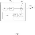
- Figure 1 shows a schematic representation of a distributed fibre optic sensing arrangement.
- a length of sensing fibre 101 is removably connected at one end to an interrogator unit 100.
- the sensing fibre 101 is coupled to an output/input of the interrogator unit 100 using conventional fibre optic coupling means.
- the interrogator unit 100 is arranged to launch pulses of coherent optical radiation into the sensing fibre 101 and to detect any radiation from said pulses which is backscattered within the optical fibre 101.
- the interrogator unit 100 will detect radiation which has been Rayleigh backscattered from within the fibre 101.
- the interrogator unit 100 comprises at least one laser 102.
- the output of the laser 102 is received by an optical modulator 103 which generates the pulse configuration as will be described later.
- the pulses output from the optical modulator 103 are then transmitted into the sensing fibre 101, for instance via a circulator 104.
- An alternative to using an optical modulator would be to drive the laser in such a way that it produces a pulsed output.
- optical is not restricted to the visible spectrum and optical radiation includes infrared radiation, ultraviolet radiation and other regions of the electromagnetic spectrum.
- a proportion of the light in the fibre 101 is backscattered from scattering sites within the fibre 101.
- the number of scattering sites can be thought to determine the amount of scattering that could occur and the distribution of such scattering sites determines the interference.
- a stimulus may result in a change of optical path length within the relevant section of fibre (which could be a physical change in length and/or a change in the effective refractive index in part of the fibre). In this simple model, this can be thought of as changing the separation of the scattering sites but without any significant effect on the number. The result is a change in interference characteristics. In effect, the stimulus leading to optical path length changes in the relevant section of fibre can be seen as varying the bias point of a virtual interferometer defined by the various scattering sites within that section of fibre 101.
- any optical radiation which is backscattered from the optical pulses propagating within the sensing fibre 101 is directed to at least one photodetector 105, again for instance via the circulator 104.
- the detector output is sampled by an analogue to digital converter (ADC) 106 and the samples from the ADC 106 are passed to processing circuitry 107 for processing.
- the processing circuitry 107 processes the detector samples to determine an output value for each of a plurality of analysis bins, each analysis bin or channel corresponding to a different (albeit possibly overlapping) longitudinal sensing portion of interest of optical fibre 101.
- the interrogator unit 100 may comprise various other components such as amplifiers, attenuators, additional filters, noise compensators, etc. but such components have been omitted in Figure 1 for clarity in explaining the general function of the interrogator unit 100.
- the laser 102 and modulator 103 are configured to produce at least one series of pulse pairs at a particular launch rate as now discussed in relation to Figure 2 .
- other pulse configurations are possible.
- Figure 2 shows a first pulse 201 at a first frequency F1 and having a duration d1 followed a short time later by a second pulse 202 having a second frequency F2 and having a second duration d2.
- the frequencies of the two pulses F1, F2 may be the same, or may differ.
- the durations (and hence the spatial widths) of the two pulses d1, d2 are equal to one another although this need not be the case.
- the two pulses 201, 202 have a separation in time equal to Ts (as shown Ts represents the time separation between the leading edges of the pulses).
- the backscatter signal received at the detector 105 at any instant is an interference signal resulting from the combination of the scattered light.
- the distributed fibre optic sensor of Figure 1 relies on the fact that any disturbance to the optical fibre e.g. strain, or thermal expansion or changes in refractive index due to temperature changes in the optical fibre 101 will cause an optical path length change which can therefore phase modulate the interference signal generated. Detecting a phase change in the interference signal from a particular section of fibre 101 can thus be used as an indication of an optical path length change upon the optical fibre 101 and hence as an indication of conditions (temperature, strain, acoustic etc) at that section of fibre 101.
- Such phase based sensors have the advantage of providing a linear and quantitative response to an incident stimulus. In principle, a series of single pulses could be used but in that case there would not be a quantitative relation between the output signal and the stimulus.
- the interrogator unit 100 is operated substantially as is described in greater detail in our previously filed applications WO2012/134022 and WO2012/134021 , which are incorporated herein by reference to the full extent allowable.
- channels are defined by a certain sampling time after launch of a pulse pair, and the successive detector outputs provide a phase modulated carrier signal at a frequency defined by the frequency difference between the pulses of a pulse pair (and therefore comprising an interference signal between light backscattered from both pulses of a pair), which may be obtained, for example, by using the modulator 103 to modulate the frequency between launching the pulses within a pulse pair.
- the carrier frequency is arranged to be one quarter of the launch rate such that a signal at the carrier frequency evolves by 90° in phase between launch of successive pulse pairs. This also allows for efficient use of modulation bandwidth.
- Figure 3 illustrates one embodiment of how this modulated carrier signal is processed by processing circuitry 107 to determine the phase of the carrier signal for a single channel.
- the samples representing the modulated carrier signal for one channel of the sensor are high pass filtered 301 to remove any components at DC or low frequency.
- the filtered signal is divided into two processing channels and the signals in each channel are multiplied by either sine 302 or cosine 303 functions at the carrier frequency and then low pass filtered by I and Q component low pass filters 304 and 305 to generate In-phase (I) and quadrature (Q) components as is known in complex demodulation schemes.
- I and Q component low pass filters 304 and 305 to generate In-phase (I) and quadrature (Q) components as is known in complex demodulation schemes.
- the carrier frequency is 1 ⁇ 4 of the ping rate
- each sample is multiplied by either 0, +1 or -1.
- the resultant I and Q signals are then used to calculate the phase value by rectangular to polar (RP) conversion 306.
- the RP conversion may optionally also generate an amplitude value.
- the output signal is a phase shift measured in radians over the frequency range from 0 Hz to an upper limit that is determined by I and Q component low pass filters 304 and 305.
- this phase shift, ⁇ 0 may be high pass filtered. This is considered advantageous as it eliminates unwanted noise signals that lie in the low frequency region.
- the phase value may be (optionally) low pass filtered to remove acoustic effects and to that end (in a departure from the teaching of WO2012/134022 and WO2012/134021 ), the data is passed to a low pass filter 307.
- the cut off frequency of the low pass filter 307 is preferably predetermined but it will be appreciated by the skilled person that there is no well defined distinction between acoustic signals and temperature signals. However typically the boundary between them is taken to be somewhere between 0.1 and 1 Hz, although other ranges including for example 1-10Hz (which could be considered to overlap with the acoustic range) may also be considered.
- This filtering is further described below. However, as also noted in greater detail below, it may not be required in all examples, and in some example, a different frequency band may be of interest, in which case the filter 307 may comprise one or more bandpass filters.
- the threshold of the I and Q component low pass filters 304 and 305 may be selected to isolate, or substantially isolate, the low frequency components of the phase signal, and the subsequent phase value low pass filter 307 may not be required.
- such filters may be primarily provided to remove the 'double-frequency' components generated in the mixing stage of producing the I and Q components, however they could also be used to remove any component at the carrier frequency which results from any remaining low frequency input signal being multiplied by the sin and cos terms.
- the threshold is generally set to be less than the carrier frequency.
- the low pass filters may be set to have a cut-off at 1/3 rd of the carrier signal frequency, which will preserve all signals imposing path length changes in the optical fibre at that frequency and below.
- the low pass filters 304 and 305 could instead have a much lower cut off, of for example 100Hz or lower. This also assists in improving the stability of the demodulation as now explained.
- the stability of the demodulation process depends on sufficient light having been backscattered from the two pulses to generate a carrier with sufficient carrier to noise ratio (CNR). These scattering sites are effectively distributed randomly within the fibre 101. For some sections of the fibre 101, light backscattered will tend to interfere constructively giving a large backscatter level from a pulse while for other sections there will be more destructive interference resulting in a lower backscatter level. If the backscattered light from either of the two pulses falls then the carrier level generated by mixing them together will decrease. A lower carrier level will mean that the I,Q components become noisier and if the noise level becomes too large then phase obtained from them will show a series of 2 ⁇ radian jumps thereby corrupting the data.
- CNR carrier to noise ratio
- the probability of these 2 ⁇ jumps occurring is inversely related to the total noise level on the I and Q components.
- this noise is broadband, its level can be reduced by using a lower frequency cut for filters 304 and 305 in Figure 3 . Therefore reducing this bandwidth reduces the chances of generating a 2 ⁇ jump in the data and so the stability of the demodulation process is improved.
- the task of isolating the low frequency signal can therefore be carried out by the I and Q component low pass filters 304, 305 or by the phase value low pass filter 307, or be shared between them.
- lowering the cut off threshold of the phase value filter 307 does not improve the stability of the demodulation.
- the threshold selected for filtering depends on the signal of interest.
- the filter(s) should be designed to retain all of the signal of interest. Considering the example of temperature, therefore, when designing the system, the anticipated temperature variation, and the speed with which the fibre reacts, should be considered, and an upper frequency threshold which preserves the fastest changing value of the anticipated changes.
- the temperature change may be determined from the suitably processed data by multiplying it by a predetermined temperature/phase relationship of the fibre cable.
- the temperature/phase relationship will depend on the fibre used. In general, the temperature/phase relationship for a bare fibre is well known but this is modified if extra coatings are placed on it or if it is included in a cable structure. The temperature/phase relationship for a particular cable could be calculated or experimentally measured. If the primary aim of a particular distributed sensing system based on Rayleigh backscatter in an optical fibre is to measure temperatures, a fibre with a high change in phase with temperature may be used. This could for example be obtained by using a fibre with a coating of a material (which may be a relatively thick coating to enhance the effect) with a high thermal expansion coefficient.
- phase to temperature can be done for any amplitude of signal.
- single pulse systems this is not possible due to the well-known signal fading issue.
- rate of phase and hence temperature change in a single pulse system is it possible to estimate the rate of phase and hence temperature change in a single pulse system.
- Steps may also be taken to compensate for laser phase noise and the like.
- laser phase noise is due to a slow drift in the wavelength of the laser generating the interrogating radiation. This can impose a similar phase shift as a slow acting stimulus and may therefore be difficult to distinguish from a temperature change.
- laser phase noise is less of a concern, as it is seen away from the signal band of interest.
- laser phase noise may in some embodiments be a significant component of the phase change signal at low frequencies (say, under 1 Hz).
- phase noise produces a signal that is the same throughout the fibre. Therefore, in one example, a portion of the fibre which is at least substantially shielded from at least some other slow acting changes (e.g. is in a temperature stable environment, to shield from temperature changes), and to use the backscatter signal from this shielded section of fibre to provide an indication of laser phase noise.
- laser phase noise may be estimated by calculating the mean signal returned from at least some, and possibly each, portion of the fibre (i.e. each channel).
- the signal from some (preferably most) portions of the fibre could be used to determine the mean, but signals returned from those portions which have high levels of low frequency signal from other sources such as the signal of interest or high levels of noise due to a low carrier signal could be excluded.
- steps may be taken to ensure that 'good quality' data is obtained and utilised in deriving measurement signals.
- a plurality of samples corresponding to each sensing portion of interest may be acquired (these samples may be acquired from overlapping sections of fibre) and designated as separate channels for processing.
- the channels may be combined according to a quality metric, which may be a measure of the degree of similarity of the processed data from the channels. This allows for samples which have a high noise level, for example due to fading of the carrier signal, to be disregarded, or given a low rating in the final result.
- the method described in WO2012/137021 utilises a high pass filter, which may also remove thermal information. Therefore, if it is low frequency signals which are of interest, to ensure that this information is returned but that the benefits of the method described in WO2012/137021 are maintained in the context of low frequency phase modulation, the method may be implemented without high pass filtering. Instead of choosing the channels which are most similar, the quality metric may instead be based on a determination of the level of signal at high frequency (with lower levels being favoured), or the ratio between the signal at low frequency (e.g. 2-20Hz), the signal at high frequency (with higher ratios being favoured), or the maximum differential of the signal with respect to time. These methods are not affected by the level of the DC offset and are based on the fact that most signals due to physical disturbances have a higher level at low frequencies, while the system noise, which depends on the variable carrier level, has a flatter spectrum.
- a DC offset may be added to the mean of the selected channels to give the output signal.
- the difference between the mean of the new set and the old set may be considered and the DC offset may be set to remove any step change.
- the mean of several successive samples of channels may be considered and the DC offset change may be smoothed over a number of such sample sets so that there is no step in the data, effectively tapering the data from old to the new set of channels to produce a smoother join.
- a quality metric may be determined on a rolling basis or periodically.
- the number of samples in the join region should be lower than any block length so as to ensure that the block length is such that multiple changes during the join region can be avoided. This can be controlled either by setting a minimum block length, or setting the number of samples which contribute to a join, or both, and could be predetermined or vary according to the data collected.
- demodulation failure may be identified by looking for steps of multiples of 2 ⁇ between samples. In practice, this may occur over several samples, such that the full 2 ⁇ change may be made over 5, 10 or more samples from different pulse pairs. Therefore, the threshold for detecting a change might be set below 2 ⁇ , for example 60% of a 2 ⁇ change, measured across the difference of, for example, five samples from different pulse pairs, although other thresholds and sample spacing may be appropriate depending on the data set and sample rate.
- Samples may be considered from within a time frame of, for example, a second (although other periods may be appropriate for a given sample set). If the characteristic of demodulation failure is detected, this data may simply be replaced one or more neighbouring channels which do not exhibit the characteristic. In one example, if both adjacent channels have not exhibited the characteristic, then the average of these channels may be used. If no adjacent channels are 'good', then data from the closest good channel may used. As mentioned above, it may be desirable to adjust or taper the join between data sets.
- the data may be downsampled, (for example decimated by 100).
- Such downsampling may be carried out using one or more of Finite Impulse Response (FIR) filter, through use of a signal processing tool such as the decimation tool in MATLAB or the like. Additional filtering and/or normalisation may be carried out.
- FIR Finite Impulse Response
- such a method will preserve more original data than methods using, for example, weighted averages with reference to a quality metric.
- CNR carrier to noise ratio
- sensing optical fibre 101 As use of such a sensing optical fibre 101 is relatively inexpensive, it may be deployed in a wellbore in a permanent fashion as the costs of leaving the fibre 101 in situ are not significant. The fibre 101 is therefore conveniently deployed in a manner which does not interfere with the normal operation of the well. In some embodiments a suitable fibre may be installed during the stage of well construction.
- Figure 4 schematically shows a well 400 for accessing underground hydrocarbons, having distributed fibre sensing apparatus associated therewith.
- the well 400 comprises a well shaft 402, which has a number of perforations 404.
- the perforations 404 are in the region of gas or other hydrocarbon reserves, and allow fluids to enter the shaft 402, where they rise, either under their own pressure or raised using pumps and the like, to a well head 406 where the hydrocarbon is collected and contained.
- the well 400 comprises a sensing fibre 101, which is attached to an interrogator unit 100 as described in relation to Figure 1 above, and, in this example, operated as described in relation to Figures 1 to 4 .
- the fibre 101 is interrogated with radiation to provide acoustic and/or temperature sensing.
- This returns a flow signal which may be indicative of a temperature change or of an acoustic signal at a given depth of the shaft 402, and is specifically related to the temperature/acoustic changes in the well 400 at that depth.
- a flow signal which may be indicative of a temperature change or of an acoustic signal at a given depth of the shaft 402
- it is the relatively low frequency temperature changes which are monitored.
- other frequency bands may be monitored.
- liquids can form what are known as 'slugs' in the well and, in the example of a gas well below, that term shall be taken to mean a substance which is capable of significant heat transfer or generation of acoustic signals within a well bore relative to other substances (e.g. gas) within the well.
- 'significant' can mean capable of a temperature change on the order of milliKelvin, which is nevertheless capable of being readily detected by the interrogator unit 100.
- a given volume of liquid in a well may have a greater cooling/heating effect than the same volume of gas.
- the slugs may be substantially water, oil or a mixture thereof (although it will be appreciated that the slugs will likely contain other substances, in particular mud, sand, contaminants, and the like), or may be a portion of gas with a high proportion of water.
- the temperature disturbance created by a slug can be tracked through a series of time-lapse temperature profiles of at least a portion of a well to provide a slug velocity profile over the well.
- the slug velocity may be considered to be indicative of fluid velocity, and therefore determining the slug velocity profile allows a first fluid velocity profile to be determined.
- an estimate of fluid inflow may be determined by assuming that the energy level of the signal due to inflow observed at any perforation is related to the amount of inflow.
- the amount of fluid entering the well is estimated to be proportional to the energy of a signal in a particular frequency band raised to the power of n (where the value of n depends on the well type).
- n the value of n depends on the well type.
- the well 400 is at least primarily a gas well and the method comprises monitoring the temperature variations due to slugs.
- a slug By monitoring for changes in temperature at a perforation, one can detect temperature changes which are indicative of inflow.
- a slug is likely to heat the area surrounding the perforation, which is otherwise cooled by the expanding gas. However, this need not always be the case: it is possible that the slug may be cooler than the area surrounding a perforation. In any event, as there are different mechanisms affecting the slug temperature and the temperature surrounding the perforation, they are unlikely to be in thermal equilibrium. Further, the amount of cooling by one particular slug will depend on the volume of that slug and its speed (a slower moving slug has more time to affect heat transfer).
- a model of a gas well in which a group of slugs 502 progress up a well shaft, may be developed.
- a slug 502 passes a perforation 404, there is a temperature change, which is detected by the interrogator unit 100.
- the temperature at the fibre 101 portion adjacent to the perforation will usually increase then decrease as the slug travels to and past the perforation region.
- the sequence of slugs 502 create oscillatory temperature changes 512.
- the path of a given slug (which for the purpose of example is a large slug 502') can be tracked past each perforation 404, in this case (as it is relatively large) as a larger temperature change.
- the time offset between detections i.e. the gradient of 504 is an indication of the speed of the slug (and could therefore be used to generate a fluid flow velocity profile based on slug tracking).
- FIG. 5 shows a thermal gradient 510 of the well 400 (which may have been determined for other purposes).
- the Joule Thompson cooling causes the local temperature to dip below that of the background thermal gradient.
- the amplitude of each temperature dip is related to amount of gas inflow at each perforation 404, with higher inflow generally resulting in a larger temperature dip.
- the temperature gradient 510 and the dips dT 1-3 are not to scale and amplitude of the dips has been exaggerated on this figure for clarity. In some cases, especially for perforations with low inflow, they may be difficult to distinguish from other localised variations in the thermal gradient 510.
- DAS i.e. Rayleigh backscattering based sensing principles are used (and are sensitive enough to detect these temperature changes), alternative temperature sensing techniques could be used.
- slugs 502 are shown as regular formations, each spanning the whole cross section of the well, the skilled person will be aware that this may not be the case. Slugs may occupy only part of the cross section, in some examples having an annular form (which may or may not be a complete annulus) in contact with the walls of the well 400.
- the thermal gradient 510 provides an 'equilibrium' temperature for each point in the well, i.e. the temperature that the well would have absent of any fluid flow.
- the thermal gradient is used for many purposes in relation to a well, including as a baseline for temperature excursions, but also for geological surveys, determining the conductivity of substances such as brine at a given depth, etc.
- the thermal gradient may be measured (for example during production of the well, during shut-in periods, or through repeated logging runs) or may be estimated based on, for example, the known thermal gradient in the region, the composition of the ground surrounding the well, or the like.
- the signal magnitude corresponds to the temperature change caused by the passing slugs 502 which in turn is related to the heat transfer and is due to a combination of factors. These factors include the cooling effect of gas inflow and therefore the volume of gas entering the well at a given perforation 404, as a larger cooling will result in a greater difference between the temperature of the slug and the perforation. It will also depend on the heat transfer capabilities of the slug which will be related to the amount of liquid in it. Thus signals at the lowest perforation 404 in the figure which has a larger degree of cooling (i.e. is associated with a relatively large dip dT 1 ) will be greater than those in the middle perforation 404 where the cooling is less (i.e. it is associated with a relatively small dip dT 2 ).
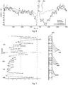
- Figure 6 shows the signals due to temperature changes gathered at a single perforation over time (solid line 602) along with the temperature signals gathered at a location which is between perforations (dotted line 604). It can be seen that the signal between perforations is less variable than the signal at the perforation.
- the signal between the perforations is smaller, there is nevertheless an appreciable signal. This is due to the temperature difference between the well and the passing slugs 502. A slug 502 having moved up from further down the well will generally be warmer than the background thermal gradient 510 of the well. At a perforation 404 the temperature will generally be less than this background gradient 510 due to the effect of gas inflow so the temperature difference between the slug 502 and the well 400 will be greater than at locations between perforations 404 where the well temperature will be closer, or at the temperature associated with the background thermal gradient. Thus the signals from between perforations 404 will tend to be smaller than those obtained at perforations 404.
- the temperature fluctuations can be used to give a measure of signal size (e.g. an indication of the sum of the temperature excursions) at various points over a well.
- Example data is shown in Figure 7 , in which signals at perforations marked with an X can be compared the signal levels between perforations marked with a O. This gives rise to set of signals (the signals at each perf, S perf n , and the signals between the perforations, S null n ).
- the peaks and troughs providing these signals can be identified at least in part from the known location of the perforations 404, or could be identified from analysis of the signals to identify the peaks or a combination of these techniques (and/or other techniques) could be used. Knowledge of other factors which may contribute to the signal allows them to be filtered out or ignored if possible.
- the data shown in Figure 7 is produced by integrating the signal energy in a frequency band that captures the temperature oscillations associated with the slug flow passage (although a different frequency band could be used in other examples). This could be achieved by summing a Fast Fourier Transform FFT in the frequency range or obtaining the RMS of the data after filtering to the desired frequency range.
- the signal level data was calculated by taking a RMS power level after high pass filtering at 0.003Hz to remove any slow drifts in the DC level of the data (for example, the well may be gradually cooling or warming).
- the threshold was set to 0.003Hz
- the frequency threshold may be determined on the basis of an individual well in a given state by examining the data and estimating the frequency of the temperature oscillation caused by the slugs, which is related to slug velocity, and ensuring this information is maintained.
- the actual temperature signal may be seen at lower frequencies, there will be a significant signal at this frequency range, and it has been noted that this signal will also be amplified at the perforations.
- low pass filtering may be desirable in some embodiments to remove acoustic signals for example, this may not always be necessary.
- the cause of these signals is the interaction of the slugs with the surroundings.
- the magnitude of temperature change will be related both to the temperature difference between the slugs and the surroundings at the point in the well and to the volume of water. Further, while more water may be added at each perforation 404, under normal conditions, little or no water will be lost.
- dT perf n the departure from the temperature that might be expected in a steady state condition given the well's thermal gradient (which, as noted above, is related to the volume of gas introduced into the well at that perforation)
- dT slug is the difference between the temperature of the slug and the steady state well temperature
- W perf n is the water from a given perforation (summed to give the total amount of water available for thermal conduction)
- k is a constant.
- the signal is also dependent on the velocity of the slug, but this is assumed to be constant over a portion of well under consideration (or the length of each section considered is limited to that over which the velocity can, to a good approximation, be considered as constant). Otherwise, the slug velocity could be included in the model.
- This equation has several terms of interest: if the dT perf n term could be found, this could be used to give a measure of production of gas at perforation n, which would be of use to a well operator. Second, if the W perf n terms could be found, this might identify the perforations which are introducing excessive amounts of water into the well 400.
- equation 1 cannot be solved analytically, as it contains too many unknown variables.
- dT slug it will be appreciated that it is difficult to measure dT slug absolutely, as it is unlikely that the fibre 101 will come into thermal equilibrium with a slug 502 due to its finite transit time.
- considering the signal between the perforation provides additional information.
- the thermal gradient in a well means that a slug travels from a hotter region to a cooler region, and in doing so deposits heat. Therefore, it could also be considered that the term kdT slug will be related to the thermal gradient. Indeed, it may be, to a reasonable approximation, proportional to the thermal gradient. Whilst this is not essential, in some examples the thermal gradient will be known (or can be readily determined by the skilled person using known techniques). This could be carried out at just some of the nulls, and could be used to inform the best-fit process. Indeed, it may be possible to solve this for all nulls, which could allow an absolute solution (i.e. analytical rather than numerical) to the inflow.
- the best fit solution could be constrained according to other known (or estimated) features of the gas well. In particular, it could be assumed that none of the water or gas terms will be negative, as in practice little to no water or gas should escape the well bore, so one constraint might be that no such terms are negative.
- DTS Distributed Temperature Sensing
- the method is preferably employed over a section of the well which is sufficiently far from the bottom of the well to avoid risk that the data could be influenced by standing water.
- the best fit solution is sensitive to the initial amount of water. In particular, if the lowermost perforation injects a large amount of water, it may be that subsequent water terms may not be readily distinguishable. Therefore, a supplementary technique, such as a known flow monitoring technique could be used in particular to inform the model at the base of the well (although they could also be used throughout the well).
- a supplementary technique such as a known flow monitoring technique could be used in particular to inform the model at the base of the well (although they could also be used throughout the well).
- the method may be preferred to start the method as far down the well as possible, before significant water inflow. More generally, the amount of water at the base of the well may be considered when assessing the confidence in the model. For example, a well which appears to be producing more water from higher than from lower perforations may be considered with a higher degree of confidence as to its accuracy than if the reverse is true.
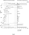
- Figure 8 shows how the proportions of gas and liquid introduced at particular perforations for a given well, using the data first presented in Figure 7 .
- the peaks and troughs identified and indicative of the gas and water contributions at each perforation can be determined, as shown on the bar chart to the right of Figure 8 . It should be noted that these are not absolute measurements, but are instead proportional contributions (and the gas and water bars are not on the same scale). The absolute values could be obtained by considering actual totals of gas and water production, as will generally be measured at the point of extraction.
- a fluid flow velocity profile of the well based on fluid inflow may be determined, noting that the fluid flow velocity at a given point in the well will be approximately proportional to the total rate of fluid entry that occurs at any point further down. Dividing this rate by the cross-section area of the well gives an estimated flow speed, which in turn can be used to provide an estimated fluid flow velocity profile.
- a separate velocity profile can be formed based on tracking a slug in a well.
- slug is rarely in thermal equilibrium with its surroundings, it can tracked by following a disturbance in a temperature profile over time.
- Figure 9 shows a 'waterfall' plot, indicating temperatures at various times t 1 to t 5 over at least a portion of a well.
- the temperature measurement may be, for example, derived from Rayleigh backscatter at a frequency of interest (which may be at the lower end of the acoustical range, (e.g. 0.3-1 Hz in some wells) or lower).
- a different frequency band may be tracked, and a feature caused by, for example, an acoustic signal indicative of turbulence, pressure or vibration due to a slug could be tracked as the slug moves up the well to provide an indication of slug velocity.
- the position of the 'disturbance' moves up the well between captured temperature profiles, allowing a slug velocity to be determined, and this can be used to provide a fluid flow velocity profile by equating slug velocity to fluid flow velocity.
- the fluid velocity profiles for a portion of the well are considered.
- this is defined using channels of the fibre monitoring system, which equate to physical lengths of fibre, and therefore in this example a length of the well bore (i.e. in this example, the fibre is arranged linearly along the well bore, although other fibre arrangements could also be used). Therefore, in this example, a section of the well corresponding to N channels is selected.
- a channel may for example correspond to between around 1 and 100 metres of fibre.
- the slug velocity is obtained by determining how long it takes for the slug to move along the N selected channels.
- N used in these calculations may be selected bearing in mind that selection of a larger value means that a more accurate value of slug velocity can be calculated but also means that the average speed over a longer distance is obtained, and therefore the precision decreases. In some examples, it may be preferable to select N such that the depth of the well represented by the N channels may be substantially equal or less than the spacing between the perforations although for wells with tightly packed perforations this may not be possible.
- the determined slug velocity is assigned to the central channel in the block of N (i.e. is assumed to be the slug velocity when the slug passes the central channel).
- the first velocity profile V slug is obtained by repeating this calculation every P channels along the fibre.
- P may be around N/2 so that there is a 50% overlap between channels used to calculate successive values of the slug velocity, although other values of P such as N/4 might also be used.
- the second inflow profile, V inflow is generated by considering the estimated inflow from each of the perforations in the well.
- the fluid velocity at any channel is considered to be proportional to the sum of the inflow at all perforations below the depth represented by that channel.
- Both profiles are then interpolated to provide intermediate values.
- the values may have a spacing which is an order of magnitude less than the typical perforation spacing, for example 1 metre spacing (i.e. to give an estimated fluid velocity every metre within the portion of the well under consideration), and the resulting values are subjected to a low pass filter, to smooth the profiles over a length scale that would typically contain a number of perforations. This number of perforations might typically be 3 or 4 although other numbers might also be chosen.
- the filtered velocity profiles are termed V* slug and V* inflow herein.
- the resulting profiles are shown in Figure 10A . As can be seen, they agree well in the lower section of the well portion, but diverge over the upper section. It will be appreciated that the filtering process may have little effect (and may therefore be neglected in other examples) on V slug , as V slug is already relatively smooth in this example as it is the average velocity over N channels.
- V combined V inf low ⁇ V slug ⁇ m V inf low ⁇ m
- each element of an array comprising the interpolated V inflow values is multiplied by the ratio of the corresponding array element in V* slug and V* inflow raised to the power of m.
- Figure 10B shows the inflow at each perforation that is calculated from V combined for three example values of m.
- the inflows for the three values of m there is little difference between the inflows for the three values of m and this is because, as shown in Figure 10A , the velocities obtained from slug motion and the inflow are similar.
- V* slug is less than V* inflow indicating that, as the value of m increases, the estimated inflow from each perforation decreases as the V combined becomes more closely coupled to V* slug rather than V* inflow .
- the inflow information calculated as described herein could form part of a well management system, which may consider other factors or measurements.
- thermometers may be positioned within the well, either in place of or to supplement the 'DAS' temperature techniques described herein.
- other frequency bands i.e. those indicative of signals which are not primarily thermal signals
- indeed alternative apparatus may be used.
Landscapes
- Physics & Mathematics (AREA)
- Engineering & Computer Science (AREA)
- Geology (AREA)
- Life Sciences & Earth Sciences (AREA)
- Mining & Mineral Resources (AREA)
- Fluid Mechanics (AREA)
- Remote Sensing (AREA)
- Environmental & Geological Engineering (AREA)
- General Life Sciences & Earth Sciences (AREA)
- Geochemistry & Mineralogy (AREA)
- Geophysics (AREA)
- General Physics & Mathematics (AREA)
- Electromagnetism (AREA)
- Health & Medical Sciences (AREA)
- Toxicology (AREA)
- Investigating Or Analysing Materials By Optical Means (AREA)
- Investigating Or Analyzing Materials By The Use Of Ultrasonic Waves (AREA)
- Measuring Temperature Or Quantity Of Heat (AREA)
- Arrangements For Transmission Of Measured Signals (AREA)
- Measuring Volume Flow (AREA)
- Sampling And Sample Adjustment (AREA)
- Testing Or Calibration Of Command Recording Devices (AREA)
Applications Claiming Priority (2)
| Application Number | Priority Date | Filing Date | Title |
|---|---|---|---|
| GBGB1408131.9A GB201408131D0 (en) | 2014-05-08 | 2014-05-08 | Fluid inflow |
| PCT/GB2015/051357 WO2015170113A1 (en) | 2014-05-08 | 2015-05-08 | Fluid inflow |
Publications (2)
| Publication Number | Publication Date |
|---|---|
| EP3140509A1 EP3140509A1 (en) | 2017-03-15 |
| EP3140509B1 true EP3140509B1 (en) | 2020-08-19 |
Family
ID=51032418
Family Applications (2)
| Application Number | Title | Priority Date | Filing Date |
|---|---|---|---|
| EP15721811.6A Active EP3140510B1 (en) | 2014-05-08 | 2015-05-08 | Fluid inflow |
| EP15721810.8A Active EP3140509B1 (en) | 2014-05-08 | 2015-05-08 | Fluid inflow |
Family Applications Before (1)
| Application Number | Title | Priority Date | Filing Date |
|---|---|---|---|
| EP15721811.6A Active EP3140510B1 (en) | 2014-05-08 | 2015-05-08 | Fluid inflow |
Country Status (9)
| Country | Link |
|---|---|
| US (2) | US10422677B2 (no) |
| EP (2) | EP3140510B1 (no) |
| CN (2) | CN106460502B (no) |
| AU (2) | AU2015257488B2 (no) |
| BR (1) | BR112016025899B1 (no) |
| CA (2) | CA2947665C (no) |
| GB (1) | GB201408131D0 (no) |
| MY (2) | MY186645A (no) |
| WO (2) | WO2015170115A1 (no) |
Families Citing this family (27)
| Publication number | Priority date | Publication date | Assignee | Title |
|---|---|---|---|---|
| US10808521B2 (en) | 2013-05-31 | 2020-10-20 | Conocophillips Company | Hydraulic fracture analysis |
| NL2014518B1 (en) * | 2015-03-25 | 2017-01-17 | Fugro Tech Bv | A device for measuring fluid parameters, a method for measuring fluid parameters and a computer program product. |
| US10890058B2 (en) * | 2016-03-09 | 2021-01-12 | Conocophillips Company | Low-frequency DAS SNR improvement |
| US20170260839A1 (en) * | 2016-03-09 | 2017-09-14 | Conocophillips Company | Das for well ranging |
| US10095828B2 (en) * | 2016-03-09 | 2018-10-09 | Conocophillips Company | Production logs from distributed acoustic sensors |
| AU2017246521B2 (en) | 2016-04-07 | 2023-02-02 | Bp Exploration Operating Company Limited | Detecting downhole sand ingress locations |
| BR112018070565A2 (pt) | 2016-04-07 | 2019-02-12 | Bp Exploration Operating Company Limited | detecção de eventos de fundo de poço usando características de domínio da frequência acústicas |
| CN106197586B (zh) * | 2016-06-23 | 2020-10-16 | 北京蔚蓝仕科技有限公司 | 井下流体的流量的测量方法和装置 |
| WO2018156099A1 (en) * | 2017-02-21 | 2018-08-30 | Halliburton Energy Services, Inc. | Distributed acoustic sensing system with phase modulator for mitigating faded channels |
| EP3583296B1 (en) | 2017-03-31 | 2021-07-21 | BP Exploration Operating Company Limited | Well and overburden monitoring using distributed acoustic sensors |
| EA202090528A1 (ru) | 2017-08-23 | 2020-07-10 | Бп Эксплорейшн Оперейтинг Компани Лимитед | Обнаружение мест скважинных пескопроявлений |
| EP3695099A2 (en) | 2017-10-11 | 2020-08-19 | BP Exploration Operating Company Limited | Detecting events using acoustic frequency domain features |
| EP3676479B1 (en) | 2017-10-17 | 2024-04-17 | ConocoPhillips Company | Low frequency distributed acoustic sensing hydraulic fracture geometry |
| US10690552B2 (en) * | 2017-12-06 | 2020-06-23 | Baker Hughes, A Ge Company, Llc | DTS performance improvement through variable mode path length averaging |
| EP3775486A4 (en) | 2018-03-28 | 2021-12-29 | Conocophillips Company | Low frequency das well interference evaluation |
| CA3097930A1 (en) | 2018-05-02 | 2019-11-07 | Conocophillips Company | Production logging inversion based on das/dts |
| US11125077B2 (en) * | 2018-07-23 | 2021-09-21 | Exxonmobil Upstream Research Company | Wellbore inflow detection based on distributed temperature sensing |
| US11859488B2 (en) | 2018-11-29 | 2024-01-02 | Bp Exploration Operating Company Limited | DAS data processing to identify fluid inflow locations and fluid type |
| GB201820331D0 (en) | 2018-12-13 | 2019-01-30 | Bp Exploration Operating Co Ltd | Distributed acoustic sensing autocalibration |
| AU2020247722B2 (en) | 2019-03-25 | 2024-02-01 | Conocophillips Company | Machine-learning based fracture-hit detection using low-frequency DAS signal |
| WO2021073741A1 (en) * | 2019-10-17 | 2021-04-22 | Lytt Limited | Fluid inflow characterization using hybrid das/dts measurements |
| CA3154435C (en) * | 2019-10-17 | 2023-03-28 | Lytt Limited | Inflow detection using dts features |
| WO2021093974A1 (en) | 2019-11-15 | 2021-05-20 | Lytt Limited | Systems and methods for draw down improvements across wellbores |
| EP4165284A1 (en) * | 2020-06-11 | 2023-04-19 | Lytt Limited | Systems and methods for subterranean fluid flow characterization |
| CA3182376A1 (en) | 2020-06-18 | 2021-12-23 | Cagri CERRAHOGLU | Event model training using in situ data |
| US20220186612A1 (en) * | 2020-12-14 | 2022-06-16 | Halliburton Energy Services, Inc. | Apparatus And Methods For Distributed Brillouin Frequency Sensing Offshore |
| EP4370780A1 (en) | 2021-07-16 | 2024-05-22 | ConocoPhillips Company | Passive production logging instrument using heat and distributed acoustic sensing |
Family Cites Families (16)
| Publication number | Priority date | Publication date | Assignee | Title |
|---|---|---|---|---|
| GB9916022D0 (en) | 1999-07-09 | 1999-09-08 | Sensor Highway Ltd | Method and apparatus for determining flow rates |
| GB2414837B (en) * | 2003-02-27 | 2006-08-16 | Schlumberger Holdings | Determining an inflow profile of a well |
| US8146656B2 (en) * | 2005-09-28 | 2012-04-03 | Schlumberger Technology Corporation | Method to measure injector inflow profiles |
| US7472594B1 (en) * | 2007-06-25 | 2009-01-06 | Schlumberger Technology Corporation | Fluid level indication system and technique |
| CN101818640A (zh) * | 2010-02-01 | 2010-09-01 | 哈尔滨工业大学 | 一种基于拉曼散射光时域反射计的油水井井下工况温度的全分布式监测装置及监测方法 |
| KR101788062B1 (ko) | 2011-03-27 | 2017-10-19 | 엘지전자 주식회사 | 네트워크 또는 디바이스를 서비스하는 관리기기의 서비스 전환 방법 |
| GB2489749B (en) | 2011-04-08 | 2016-01-20 | Optasense Holdings Ltd | Fibre optic distributed sensing |
| CN102364046B (zh) * | 2011-08-18 | 2014-04-02 | 西北工业大学 | 一种用于井下管道的多相流量计 |
| GB201116816D0 (en) | 2011-09-29 | 2011-11-09 | Qintetiq Ltd | Flow monitoring |
| CN202381084U (zh) * | 2011-12-06 | 2012-08-15 | 中国石油天然气股份有限公司 | 同光纤温度压力组合监测系统 |
| WO2013084183A2 (en) * | 2011-12-06 | 2013-06-13 | Schlumberger Technology B.V. | Multiphase flowmeter |
| CN202451145U (zh) * | 2012-01-17 | 2012-09-26 | 北京奥飞搏世技术服务有限公司 | 基于光纤传感的煤层气井压力、温度监测系统 |
| CN202483554U (zh) * | 2012-03-29 | 2012-10-10 | 东北石油大学 | 油井产液光纤计量系统 |
| CN102943620B (zh) * | 2012-08-27 | 2013-08-28 | 中国石油大学(华东) | 基于钻井环空井筒多相流动计算的控压钻井方法 |
| US9239406B2 (en) * | 2012-12-18 | 2016-01-19 | Halliburton Energy Services, Inc. | Downhole treatment monitoring systems and methods using ion selective fiber sensors |
| US10865818B2 (en) * | 2016-05-06 | 2020-12-15 | Virginia Tech Intellectual Properties, Inc. | Generalized flow profile production |
-
2014
- 2014-05-08 GB GBGB1408131.9A patent/GB201408131D0/en not_active Ceased
-
2015
- 2015-05-08 AU AU2015257488A patent/AU2015257488B2/en not_active Ceased
- 2015-05-08 CN CN201580037082.XA patent/CN106460502B/zh not_active Expired - Fee Related
- 2015-05-08 WO PCT/GB2015/051359 patent/WO2015170115A1/en active Application Filing
- 2015-05-08 EP EP15721811.6A patent/EP3140510B1/en active Active
- 2015-05-08 CN CN201580037035.5A patent/CN106471210B/zh not_active Expired - Fee Related
- 2015-05-08 US US15/307,562 patent/US10422677B2/en active Active
- 2015-05-08 MY MYPI2016704057A patent/MY186645A/en unknown
- 2015-05-08 CA CA2947665A patent/CA2947665C/en active Active
- 2015-05-08 AU AU2015257490A patent/AU2015257490B2/en not_active Ceased
- 2015-05-08 WO PCT/GB2015/051357 patent/WO2015170113A1/en active Application Filing
- 2015-05-08 BR BR112016025899-1A patent/BR112016025899B1/pt active IP Right Grant
- 2015-05-08 EP EP15721810.8A patent/EP3140509B1/en active Active
- 2015-05-08 CA CA2947516A patent/CA2947516C/en active Active
- 2015-05-08 US US15/307,571 patent/US10578472B2/en active Active
- 2015-05-08 MY MYPI2016704059A patent/MY186653A/en unknown
Non-Patent Citations (1)
| Title |
|---|
| None * |
Also Published As
| Publication number | Publication date |
|---|---|
| CN106460502B (zh) | 2019-12-17 |
| CN106471210A (zh) | 2017-03-01 |
| US10578472B2 (en) | 2020-03-03 |
| CA2947665A1 (en) | 2015-11-12 |
| AU2015257488B2 (en) | 2019-06-13 |
| US20170052050A1 (en) | 2017-02-23 |
| EP3140510B1 (en) | 2019-07-31 |
| AU2015257488A1 (en) | 2016-11-10 |
| BR112016025899A2 (no) | 2017-08-15 |
| CN106471210B (zh) | 2019-12-17 |
| CA2947516A1 (en) | 2015-11-12 |
| US20170052049A1 (en) | 2017-02-23 |
| MY186645A (en) | 2021-08-02 |
| CA2947516C (en) | 2022-02-08 |
| CA2947665C (en) | 2022-06-07 |
| WO2015170113A1 (en) | 2015-11-12 |
| CN106460502A (zh) | 2017-02-22 |
| US10422677B2 (en) | 2019-09-24 |
| MY186653A (en) | 2021-08-04 |
| WO2015170115A1 (en) | 2015-11-12 |
| AU2015257490B2 (en) | 2019-08-08 |
| BR112016025899B1 (pt) | 2022-02-22 |
| EP3140510A1 (en) | 2017-03-15 |
| GB201408131D0 (en) | 2014-06-25 |
| AU2015257490A1 (en) | 2016-11-10 |
| EP3140509A1 (en) | 2017-03-15 |
Similar Documents
| Publication | Publication Date | Title |
|---|---|---|
| EP3140509B1 (en) | Fluid inflow | |
| US10196890B2 (en) | Method of acoustic surveying | |
| EP3140630B1 (en) | Fibre optic distributed sensing | |
| EP1196743B1 (en) | Method and apparatus for determining flow rates | |
| EP3427017B1 (en) | Production logs from distributed acoustic sensors | |
| Paleja et al. | Velocity tracking for flow monitoring and production profiling using distributed acoustic sensing | |
| US10656041B2 (en) | Detection of leaks from a pipeline using a distributed temperature sensor | |
| AU2010309577A1 (en) | Downhole monitoring with distributed acoustic/vibration, strain and/or density sensing | |
| CN108369118A (zh) | 使用光纤传感器对明渠中的流体流的监测 | |
| Yamate | Fiber-optic sensors for the exploration of oil and gas | |
| RU2298094C2 (ru) | Способ обнаружения полезных ископаемых | |
| Sidenko et al. | Compensation of the temperature effect on low-frequency DAS measurements: Case study of the water injection at the Otway site | |
| RU2806672C1 (ru) | Способ определения заколонного перетока жидкости в действующих скважинах | |
| Ahmed | Critical Analysis and Application of Optical Fiber Sensors in Oil and Gas Industry. |
Legal Events
| Date | Code | Title | Description |
|---|---|---|---|
| STAA | Information on the status of an ep patent application or granted ep patent |
Free format text: STATUS: THE INTERNATIONAL PUBLICATION HAS BEEN MADE |
|
| PUAI | Public reference made under article 153(3) epc to a published international application that has entered the european phase |
Free format text: ORIGINAL CODE: 0009012 |
|
| STAA | Information on the status of an ep patent application or granted ep patent |
Free format text: STATUS: REQUEST FOR EXAMINATION WAS MADE |
|
| 17P | Request for examination filed |
Effective date: 20161130 |
|
| AK | Designated contracting states |
Kind code of ref document: A1 Designated state(s): AL AT BE BG CH CY CZ DE DK EE ES FI FR GB GR HR HU IE IS IT LI LT LU LV MC MK MT NL NO PL PT RO RS SE SI SK SM TR |
|
| AX | Request for extension of the european patent |
Extension state: BA ME |
|
| DAV | Request for validation of the european patent (deleted) | ||
| DAX | Request for extension of the european patent (deleted) | ||
| STAA | Information on the status of an ep patent application or granted ep patent |
Free format text: STATUS: EXAMINATION IS IN PROGRESS |
|
| 17Q | First examination report despatched |
Effective date: 20180503 |
|
| GRAP | Despatch of communication of intention to grant a patent |
Free format text: ORIGINAL CODE: EPIDOSNIGR1 |
|
| STAA | Information on the status of an ep patent application or granted ep patent |
Free format text: STATUS: GRANT OF PATENT IS INTENDED |
|
| INTG | Intention to grant announced |
Effective date: 20200318 |
|
| GRAS | Grant fee paid |
Free format text: ORIGINAL CODE: EPIDOSNIGR3 |
|
| GRAA | (expected) grant |
Free format text: ORIGINAL CODE: 0009210 |
|
| STAA | Information on the status of an ep patent application or granted ep patent |
Free format text: STATUS: THE PATENT HAS BEEN GRANTED |
|
| AK | Designated contracting states |
Kind code of ref document: B1 Designated state(s): AL AT BE BG CH CY CZ DE DK EE ES FI FR GB GR HR HU IE IS IT LI LT LU LV MC MK MT NL NO PL PT RO RS SE SI SK SM TR |
|
| REG | Reference to a national code |
Ref country code: CH Ref legal event code: EP |
|
| REG | Reference to a national code |
Ref country code: DE Ref legal event code: R096 Ref document number: 602015057669 Country of ref document: DE |
|
| REG | Reference to a national code |
Ref country code: AT Ref legal event code: REF Ref document number: 1304139 Country of ref document: AT Kind code of ref document: T Effective date: 20200915 |
|
| REG | Reference to a national code |
Ref country code: IE Ref legal event code: FG4D |
|
| REG | Reference to a national code |
Ref country code: NO Ref legal event code: T2 Effective date: 20200819 |
|
| REG | Reference to a national code |
Ref country code: LT Ref legal event code: MG4D |
|
| REG | Reference to a national code |
Ref country code: DE Ref legal event code: R082 Ref document number: 602015057669 Country of ref document: DE Representative=s name: HL KEMPNER PATENTANWAELTE, SOLICITORS (ENGLAND, DE Ref country code: DE Ref legal event code: R082 Ref document number: 602015057669 Country of ref document: DE Representative=s name: HL KEMPNER PATENTANWALT, RECHTSANWALT, SOLICIT, DE |
|
| REG | Reference to a national code |
Ref country code: NL Ref legal event code: MP Effective date: 20200819 |
|
| PG25 | Lapsed in a contracting state [announced via postgrant information from national office to epo] |
Ref country code: FI Free format text: LAPSE BECAUSE OF FAILURE TO SUBMIT A TRANSLATION OF THE DESCRIPTION OR TO PAY THE FEE WITHIN THE PRESCRIBED TIME-LIMIT Effective date: 20200819 Ref country code: GR Free format text: LAPSE BECAUSE OF FAILURE TO SUBMIT A TRANSLATION OF THE DESCRIPTION OR TO PAY THE FEE WITHIN THE PRESCRIBED TIME-LIMIT Effective date: 20201120 Ref country code: PT Free format text: LAPSE BECAUSE OF FAILURE TO SUBMIT A TRANSLATION OF THE DESCRIPTION OR TO PAY THE FEE WITHIN THE PRESCRIBED TIME-LIMIT Effective date: 20201221 Ref country code: HR Free format text: LAPSE BECAUSE OF FAILURE TO SUBMIT A TRANSLATION OF THE DESCRIPTION OR TO PAY THE FEE WITHIN THE PRESCRIBED TIME-LIMIT Effective date: 20200819 Ref country code: SE Free format text: LAPSE BECAUSE OF FAILURE TO SUBMIT A TRANSLATION OF THE DESCRIPTION OR TO PAY THE FEE WITHIN THE PRESCRIBED TIME-LIMIT Effective date: 20200819 Ref country code: LT Free format text: LAPSE BECAUSE OF FAILURE TO SUBMIT A TRANSLATION OF THE DESCRIPTION OR TO PAY THE FEE WITHIN THE PRESCRIBED TIME-LIMIT Effective date: 20200819 Ref country code: BG Free format text: LAPSE BECAUSE OF FAILURE TO SUBMIT A TRANSLATION OF THE DESCRIPTION OR TO PAY THE FEE WITHIN THE PRESCRIBED TIME-LIMIT Effective date: 20201119 |
|
| REG | Reference to a national code |
Ref country code: AT Ref legal event code: MK05 Ref document number: 1304139 Country of ref document: AT Kind code of ref document: T Effective date: 20200819 |
|
| PG25 | Lapsed in a contracting state [announced via postgrant information from national office to epo] |
Ref country code: PL Free format text: LAPSE BECAUSE OF FAILURE TO SUBMIT A TRANSLATION OF THE DESCRIPTION OR TO PAY THE FEE WITHIN THE PRESCRIBED TIME-LIMIT Effective date: 20200819 Ref country code: NL Free format text: LAPSE BECAUSE OF FAILURE TO SUBMIT A TRANSLATION OF THE DESCRIPTION OR TO PAY THE FEE WITHIN THE PRESCRIBED TIME-LIMIT Effective date: 20200819 Ref country code: RS Free format text: LAPSE BECAUSE OF FAILURE TO SUBMIT A TRANSLATION OF THE DESCRIPTION OR TO PAY THE FEE WITHIN THE PRESCRIBED TIME-LIMIT Effective date: 20200819 Ref country code: LV Free format text: LAPSE BECAUSE OF FAILURE TO SUBMIT A TRANSLATION OF THE DESCRIPTION OR TO PAY THE FEE WITHIN THE PRESCRIBED TIME-LIMIT Effective date: 20200819 Ref country code: IS Free format text: LAPSE BECAUSE OF FAILURE TO SUBMIT A TRANSLATION OF THE DESCRIPTION OR TO PAY THE FEE WITHIN THE PRESCRIBED TIME-LIMIT Effective date: 20201219 |
|
| PG25 | Lapsed in a contracting state [announced via postgrant information from national office to epo] |
Ref country code: CZ Free format text: LAPSE BECAUSE OF FAILURE TO SUBMIT A TRANSLATION OF THE DESCRIPTION OR TO PAY THE FEE WITHIN THE PRESCRIBED TIME-LIMIT Effective date: 20200819 Ref country code: DK Free format text: LAPSE BECAUSE OF FAILURE TO SUBMIT A TRANSLATION OF THE DESCRIPTION OR TO PAY THE FEE WITHIN THE PRESCRIBED TIME-LIMIT Effective date: 20200819 Ref country code: EE Free format text: LAPSE BECAUSE OF FAILURE TO SUBMIT A TRANSLATION OF THE DESCRIPTION OR TO PAY THE FEE WITHIN THE PRESCRIBED TIME-LIMIT Effective date: 20200819 Ref country code: SM Free format text: LAPSE BECAUSE OF FAILURE TO SUBMIT A TRANSLATION OF THE DESCRIPTION OR TO PAY THE FEE WITHIN THE PRESCRIBED TIME-LIMIT Effective date: 20200819 Ref country code: RO Free format text: LAPSE BECAUSE OF FAILURE TO SUBMIT A TRANSLATION OF THE DESCRIPTION OR TO PAY THE FEE WITHIN THE PRESCRIBED TIME-LIMIT Effective date: 20200819 |
|
| REG | Reference to a national code |
Ref country code: DE Ref legal event code: R097 Ref document number: 602015057669 Country of ref document: DE |
|
| PG25 | Lapsed in a contracting state [announced via postgrant information from national office to epo] |
Ref country code: AT Free format text: LAPSE BECAUSE OF FAILURE TO SUBMIT A TRANSLATION OF THE DESCRIPTION OR TO PAY THE FEE WITHIN THE PRESCRIBED TIME-LIMIT Effective date: 20200819 Ref country code: AL Free format text: LAPSE BECAUSE OF FAILURE TO SUBMIT A TRANSLATION OF THE DESCRIPTION OR TO PAY THE FEE WITHIN THE PRESCRIBED TIME-LIMIT Effective date: 20200819 Ref country code: ES Free format text: LAPSE BECAUSE OF FAILURE TO SUBMIT A TRANSLATION OF THE DESCRIPTION OR TO PAY THE FEE WITHIN THE PRESCRIBED TIME-LIMIT Effective date: 20200819 |
|
| PLBE | No opposition filed within time limit |
Free format text: ORIGINAL CODE: 0009261 |
|
| STAA | Information on the status of an ep patent application or granted ep patent |
Free format text: STATUS: NO OPPOSITION FILED WITHIN TIME LIMIT |
|
| PG25 | Lapsed in a contracting state [announced via postgrant information from national office to epo] |
Ref country code: SK Free format text: LAPSE BECAUSE OF FAILURE TO SUBMIT A TRANSLATION OF THE DESCRIPTION OR TO PAY THE FEE WITHIN THE PRESCRIBED TIME-LIMIT Effective date: 20200819 |
|
| 26N | No opposition filed |
Effective date: 20210520 |
|
| PG25 | Lapsed in a contracting state [announced via postgrant information from national office to epo] |
Ref country code: IT Free format text: LAPSE BECAUSE OF FAILURE TO SUBMIT A TRANSLATION OF THE DESCRIPTION OR TO PAY THE FEE WITHIN THE PRESCRIBED TIME-LIMIT Effective date: 20200819 |
|
| PG25 | Lapsed in a contracting state [announced via postgrant information from national office to epo] |
Ref country code: SI Free format text: LAPSE BECAUSE OF FAILURE TO SUBMIT A TRANSLATION OF THE DESCRIPTION OR TO PAY THE FEE WITHIN THE PRESCRIBED TIME-LIMIT Effective date: 20200819 |
|
| REG | Reference to a national code |
Ref country code: CH Ref legal event code: PL |
|
| PG25 | Lapsed in a contracting state [announced via postgrant information from national office to epo] |
Ref country code: LI Free format text: LAPSE BECAUSE OF NON-PAYMENT OF DUE FEES Effective date: 20210531 Ref country code: MC Free format text: LAPSE BECAUSE OF FAILURE TO SUBMIT A TRANSLATION OF THE DESCRIPTION OR TO PAY THE FEE WITHIN THE PRESCRIBED TIME-LIMIT Effective date: 20200819 Ref country code: CH Free format text: LAPSE BECAUSE OF NON-PAYMENT OF DUE FEES Effective date: 20210531 Ref country code: LU Free format text: LAPSE BECAUSE OF NON-PAYMENT OF DUE FEES Effective date: 20210508 |
|
| REG | Reference to a national code |
Ref country code: BE Ref legal event code: MM Effective date: 20210531 |
|
| PG25 | Lapsed in a contracting state [announced via postgrant information from national office to epo] |
Ref country code: IE Free format text: LAPSE BECAUSE OF NON-PAYMENT OF DUE FEES Effective date: 20210508 |
|
| PG25 | Lapsed in a contracting state [announced via postgrant information from national office to epo] |
Ref country code: BE Free format text: LAPSE BECAUSE OF NON-PAYMENT OF DUE FEES Effective date: 20210531 |
|
| PG25 | Lapsed in a contracting state [announced via postgrant information from national office to epo] |
Ref country code: HU Free format text: LAPSE BECAUSE OF FAILURE TO SUBMIT A TRANSLATION OF THE DESCRIPTION OR TO PAY THE FEE WITHIN THE PRESCRIBED TIME-LIMIT; INVALID AB INITIO Effective date: 20150508 |
|
| P01 | Opt-out of the competence of the unified patent court (upc) registered |
Effective date: 20230524 |
|
| PG25 | Lapsed in a contracting state [announced via postgrant information from national office to epo] |
Ref country code: CY Free format text: LAPSE BECAUSE OF FAILURE TO SUBMIT A TRANSLATION OF THE DESCRIPTION OR TO PAY THE FEE WITHIN THE PRESCRIBED TIME-LIMIT Effective date: 20200819 |
|
| PGFP | Annual fee paid to national office [announced via postgrant information from national office to epo] |
Ref country code: NO Payment date: 20230511 Year of fee payment: 9 Ref country code: FR Payment date: 20230509 Year of fee payment: 9 Ref country code: DE Payment date: 20230512 Year of fee payment: 9 |
|
| PGFP | Annual fee paid to national office [announced via postgrant information from national office to epo] |
Ref country code: GB Payment date: 20230517 Year of fee payment: 9 |
|
| REG | Reference to a national code |
Ref country code: DE Ref legal event code: R081 Ref document number: 602015057669 Country of ref document: DE Owner name: OPTASENSE HOLDINGS LTD., CAMBERLEY, GB Free format text: FORMER OWNER: OPTASENSE HOLDINGS LTD., FARNBOROUGH, HAMPSHIRE, GB |
|
| PG25 | Lapsed in a contracting state [announced via postgrant information from national office to epo] |
Ref country code: MK Free format text: LAPSE BECAUSE OF FAILURE TO SUBMIT A TRANSLATION OF THE DESCRIPTION OR TO PAY THE FEE WITHIN THE PRESCRIBED TIME-LIMIT Effective date: 20200819 |