EP3114645B1 - Apparatus and method for generating and using a subject-specific statistical motion model - Google Patents
Apparatus and method for generating and using a subject-specific statistical motion model Download PDFInfo
- Publication number
- EP3114645B1 EP3114645B1 EP15709309.7A EP15709309A EP3114645B1 EP 3114645 B1 EP3114645 B1 EP 3114645B1 EP 15709309 A EP15709309 A EP 15709309A EP 3114645 B1 EP3114645 B1 EP 3114645B1
- Authority
- EP
- European Patent Office
- Prior art keywords
- subject
- shape
- representations
- parameters
- specific
- Prior art date
- Legal status (The legal status is an assumption and is not a legal conclusion. Google has not performed a legal analysis and makes no representation as to the accuracy of the status listed.)
- Active
Links
Images






Classifications
-
- G—PHYSICS
- G06—COMPUTING OR CALCULATING; COUNTING
- G06T—IMAGE DATA PROCESSING OR GENERATION, IN GENERAL
- G06T7/00—Image analysis
- G06T7/10—Segmentation; Edge detection
- G06T7/12—Edge-based segmentation
-
- G—PHYSICS
- G06—COMPUTING OR CALCULATING; COUNTING
- G06T—IMAGE DATA PROCESSING OR GENERATION, IN GENERAL
- G06T7/00—Image analysis
- G06T7/10—Segmentation; Edge detection
- G06T7/143—Segmentation; Edge detection involving probabilistic approaches, e.g. Markov random field [MRF] modelling
-
- G—PHYSICS
- G06—COMPUTING OR CALCULATING; COUNTING
- G06T—IMAGE DATA PROCESSING OR GENERATION, IN GENERAL
- G06T7/00—Image analysis
- G06T7/10—Segmentation; Edge detection
- G06T7/149—Segmentation; Edge detection involving deformable models, e.g. active contour models
-
- G—PHYSICS
- G06—COMPUTING OR CALCULATING; COUNTING
- G06T—IMAGE DATA PROCESSING OR GENERATION, IN GENERAL
- G06T7/00—Image analysis
- G06T7/30—Determination of transform parameters for the alignment of images, i.e. image registration
- G06T7/33—Determination of transform parameters for the alignment of images, i.e. image registration using feature-based methods
- G06T7/344—Determination of transform parameters for the alignment of images, i.e. image registration using feature-based methods involving models
-
- G—PHYSICS
- G06—COMPUTING OR CALCULATING; COUNTING
- G06V—IMAGE OR VIDEO RECOGNITION OR UNDERSTANDING
- G06V10/00—Arrangements for image or video recognition or understanding
- G06V10/70—Arrangements for image or video recognition or understanding using pattern recognition or machine learning
- G06V10/74—Image or video pattern matching; Proximity measures in feature spaces
- G06V10/75—Organisation of the matching processes, e.g. simultaneous or sequential comparisons of image or video features; Coarse-fine approaches, e.g. multi-scale approaches; using context analysis; Selection of dictionaries
- G06V10/755—Deformable models or variational models, e.g. snakes or active contours
- G06V10/7553—Deformable models or variational models, e.g. snakes or active contours based on shape, e.g. active shape models [ASM]
-
- G—PHYSICS
- G06—COMPUTING OR CALCULATING; COUNTING
- G06T—IMAGE DATA PROCESSING OR GENERATION, IN GENERAL
- G06T2207/00—Indexing scheme for image analysis or image enhancement
- G06T2207/10—Image acquisition modality
- G06T2207/10072—Tomographic images
-
- G—PHYSICS
- G06—COMPUTING OR CALCULATING; COUNTING
- G06T—IMAGE DATA PROCESSING OR GENERATION, IN GENERAL
- G06T2207/00—Indexing scheme for image analysis or image enhancement
- G06T2207/20—Special algorithmic details
- G06T2207/20081—Training; Learning
-
- G—PHYSICS
- G06—COMPUTING OR CALCULATING; COUNTING
- G06T—IMAGE DATA PROCESSING OR GENERATION, IN GENERAL
- G06T2207/00—Indexing scheme for image analysis or image enhancement
- G06T2207/20—Special algorithmic details
- G06T2207/20112—Image segmentation details
- G06T2207/20124—Active shape model [ASM]
-
- G—PHYSICS
- G06—COMPUTING OR CALCULATING; COUNTING
- G06T—IMAGE DATA PROCESSING OR GENERATION, IN GENERAL
- G06T2207/00—Indexing scheme for image analysis or image enhancement
- G06T2207/30—Subject of image; Context of image processing
- G06T2207/30004—Biomedical image processing
- G06T2207/30081—Prostate
-
- G—PHYSICS
- G06—COMPUTING OR CALCULATING; COUNTING
- G06V—IMAGE OR VIDEO RECOGNITION OR UNDERSTANDING
- G06V2201/00—Indexing scheme relating to image or video recognition or understanding
- G06V2201/03—Recognition of patterns in medical or anatomical images
-
- G—PHYSICS
- G06—COMPUTING OR CALCULATING; COUNTING
- G06V—IMAGE OR VIDEO RECOGNITION OR UNDERSTANDING
- G06V2201/00—Indexing scheme relating to image or video recognition or understanding
- G06V2201/03—Recognition of patterns in medical or anatomical images
- G06V2201/031—Recognition of patterns in medical or anatomical images of internal organs
Definitions
- the present application relates to a method and apparatus for generating and using a subject-specific statistical motion model, such as may be used in the processing of medical images.
- Statistical shape modelling provides a powerful method to describe and compensate for physical organ shape changes, for example, due to inter-subject anatomical variation, and has been investigated extensively for a range of medical image analysis tasks, including image segmentation [1] and image registration [2].
- image segmentation [1] and image registration [2] image segmentation [1] and image registration [2].
- PCA principal component analysis
- Such models help to ensure that physically implausible organ shapes are not considered, or are at least penalised, when searching for a solution within a segmentation and registration algorithm.
- Variations in the shape of an organ can generally be considered as arising from two sources.
- the first termed inter-subject variation
- the second termed intra-subject variation
- Such intra-subject variations can be caused by many different factors, such as a change in posture of the person, natural organ motion (e.g. due to breathing or the beating heart), tissue deformation by the insertion of a medical instrument, the progression or regression of a disease, etc.
- SSMs that represent intra-subject organ motion may be termed statistical motion models (SMMs) to distinguish them from the more general SSM [6, 7].
- SMMs statistical motion models
- inter- and intra-subject shape variation is illustrated by considering the following: if we have first and second organ states, which each corresponds to a different organ shape that arises from intra-subject organ shape variation, then there must be some physical transition of the organ between the first and second states to produce the change in organ shape.
- a model of such intra-subject variation can be referred to as a SMM ( statistical motion model), since the physical transition implies a motion in a general sense (including a shape change due to organ deformation) between the first and second shapes.
- SMM statistical motion model
- the differences between the first and second organ shapes arise from inter-subject variation, then they correspond to different individuals, and there is no reason for such a physical transition to exist between the first and second shapes corresponding to some change in state. Accordingly, this type of variation is represented by a more generic SSM ( statistic shape model ), since the first and second shapes are not generally related to one another by motion.
- an SSM based at least in part on inter-subject training data, it may permit a variation that is not, in fact, physically plausible for a given organ.
- the separation between the eyes in effect, the skull size
- an SSM which is based on at least in part on inter-subject training data might potentially allow variation in this eye separation, despite the fact that such variation is not physically plausible in the context of an individual subject.
- multilinear analysis [9] has been proposed as a method for dynamic modelling of the heart [10] and cardiac valve [11] motion.
- This approach enables inter-subject shape variations (e.g., due to subject specific differences in the size and shape of the heart of different individuals) and intra-subject shape variations (e.g. due to physiological heart motion) to be represented by the same statistical model.
- this method requires that inter - subject temporal correspondence between motion subspaces is known - in other words, the states of the organs for different subjects must be correlated, for example, via an independent signal, such as an electrocardiographic (ECG) signal, which measures the electrical activity of the heart and is therefore inherently correlated to its motion.
- ECG electrocardiographic
- subject-specific dynamic data on organ motion for example, from imaging
- imaging is often extremely limited or not available at all, but many examples exist in the context of image-guided surgical procedures where it is desirable to be able provide models which use learnt information on inter- and intra-subject organ shape variation to predict subject-specific organ shape and motion given only sparse and potentially noisy (intraoperative) spatial data that describe the current organ state.
- MRI magnetic resonance imaging
- intraoperative imaging such as ultrasound
- One well-established way of overcoming this difficulty is to perform a (non-rigid) registration (i.e. spatial alignment) between the pre-operative image and the intraoperative image, thereby allowing structures determined in the pre-operative images to be mapped across to (and displayed in conjunction with) the intra-operative images.
- this is achieved using special-purpose image fusion software, and an important requirement for surgical applications is that the image registration needs to be performed within a timescale that is acceptable in the context of the surgical procedure.
- the image registration should also be able to compensate for movement and deformation in the organ or structures of surgical interest, for example, due to changes in the subject position or posture, or as a direct result of instruments used in the surgical procedure itself (for example, organ deformation arising from ultrasound imaging probe pressure).
- organ deformation arising from ultrasound imaging probe pressure.
- the physical nature of this organ motion in an individual subject suggests that an SMM approach is appropriate, but for cases where dynamic imaging is unavailable, generating a subject-specific SMM by performing biomechanical simulations of organ motion to provide training data is both a complex and time-consuming process, both computationally and from the point of view of implementing within a clinical workflow.
- the approach described herein enables a subject-specific SMM to be built without knowing the correspondence between subject subspaces - in other words, a relationship between the shapes and states of the organs of different subjects does not need to be established.
- this approach involves only limited subject-specific geometric data, for example, a reference shape based on the segmentation of one static image, to predict the organ motion for a new (unseen) subject.
- the application of this approach for deformable registration of MRI and transrectal ultrasound (TRUS) images of the prostate is discussed below.
- a new framework for statistical shape modelling of subject-specific organ motion including soft-tissue organ deformation, etc. is described herein.
- the approach adopted combines modelling of subject-specific probability of shape model parameters with kernel regression analysis to predict organ motion for an unseen subject.
- the approach is computationally efficient, uses only a limited number of training shape samples for each subject, and is highly suited to image analysis problems where prior subject-specific information on organ shape variation is useful, but where obtaining sufficient training data to construct a statistical shape/motion model for each new subject is impractical or technically or logistically difficult.
- subject-specific, MRI-derived statistical prostate motion models are generated and compared with models built using subject-specific training data provided by finite element simulations and mixed subject data that exhibits variation in shape due inter-subject variations and intra-subject prostate motion.
- the results from this investigation show that the two subject-specific models are generally equivalent in terms of output, and provide much higher specificity than can be obtained with a mixed model built using training datasets from a group of subjects.
- Some embodiments of the invention provide a method and an apparatus for building a subject-specific statistical model of shape variation for an anatomical structure using a set of geometric representations of shape for the anatomical structure.
- Each representation is associated with one of multiple subjects, each subject having a respective subset of associated representations, and each subset comprising multiple representations including a reference representation.
- the multiple representations correspond to different shapes of the anatomical structure arising from physical motion and/or deformation thereof.
- the method comprises specifying a set of shape parameters whose values, for any given representation, characterise the shape of the representation, and for each subject, representing a probability distribution of the values of the shape parameters across the subset of representations associated with that subject by a set of subject-specific distribution parameters.
- the method further comprises determining a regression between the subject-specific distribution parameters and the respective reference representation for each subject, and applying said determined regression to a reference representation for a new subject to determine subject-specific distribution parameters for the new subject.
- the subject-specific distribution parameters are then used to build a subject-specific statistical motion model for the new subject.
- the geometric representations may, for example, comprise images.
- the images may be three-dimensional, especially for representing the three-dimensional shape of the anatomical structure.
- the images may also be two dimensional; this may be appropriate, for example, in a facial recognition systems.
- the images may be obtained from one or more suitable imaging modalities, such as (without limitation) magnetic resonance imaging (MRI), X-ray computed tomography (CT), positron emission tomography (PET), ultrasound, photo-acoustic imaging (PAT), optical, X-ray or gamma ray imaging, optical microscopy, electron microscopy, etc.
- suitable imaging modalities such as (without limitation) magnetic resonance imaging (MRI), X-ray computed tomography (CT), positron emission tomography (PET), ultrasound, photo-acoustic imaging (PAT), optical, X-ray or gamma ray imaging, optical microscopy, electron microscopy, etc.
- the geometric representations may also be derived, for example, from biomechanical modelling.
- shape of an anatomical structure for a subject might initially be determined by measurement (whether from an image, or by any other appropriate physical measurement technique), and a model fitted to this shape based on known properties of the materials of the anatomical structure, such as elasticity, etc.
- the model allows the anatomical structure to move or deform in accordance with these known properties, thereby creating other physically realistic shapes for the anatomical structure.
- Representations of these shapes in effect, instances of the model corresponding to different locations across the parameter space of the model, can be utilised to provide the geometric representations of shape for the anatomical structure.
- Such geometric representations can be provided in any appropriate format, for example, as an image generated from the model, or as a set of positions of particular features or landmarks on the anatomical structure according to the configuration of that particular model instance.
- the geometrical representations may be derived from a combination of sources, for example, from multiple different imaging modalities, and/or from biomechanical modelling.
- the set of shape parameters are determined using principal component analysis (PCA), which provides a compact representation of the domain or space of the geometric representations.
- PCA principal component analysis
- other embodiments may utilise different shape parameters. For example, if the representations are derived from biomechanical modelling, then the shape parameters might potentially be derived directly from (or correspond to) the values of certain model parameters.
- the anatomical structure may represent an organ, such as the prostate, liver, kidney or heart, comprising soft tissue. Modelling of such organs is typically performed for medical reasons.
- the modelling may support a non-rigid image registration, which allows a first image to be mapped (registered) to a second image.
- the first image might be a detailed pre-operative image, such as acquired via MRI
- the second image might be an intra-operative image, such as acquired via ultrasound.
- the modelling described herein can help the non-rigid image registration to accommodate, in a computationally efficient manner, deformation or motion of the organ, such as may arise from a change in posture of the subject, the presence of a surgical instrument, some change in physiological state, and/or any other source of deformation.
- the modelling described herein can also be utilised for non-medical purposes, such as facial recognition.
- SSPDF subject-specific probability density function
- FIG. 1 A schematic overview of the method used to build a subject-specific SMM is shown in Figure 1 .
- the stages involved are as follows:
- the main steps described above are also illustrated in Figure 1 .
- the resulting subject-specific SMM is an alternative to a subject-specific SMM built directly from training data available for this subject (including image-based and simulated training data). Therefore, the subject-specific SMM estimated using this method can be compared directly with one generated using the conventional method.
- an illustration of implementing these steps is provided using the example of building a subject-specific SMM of the prostate that captures deformation caused by the placement of an ultrasound probe in the rectum.
- Figure 2 shows a schematic representation of the shapes of the prostates of I subjects, as represented by triangulated meshes.
- the shape of each mesh has been simulated using finite element (FE) modelling to predict various physical deformations of a reference shape in response to the presence of a transrectal ultrasound (TRUS) probe.
- FE finite element
- TRUS transrectal ultrasound
- the 3D position and orientation of the TRUS probe is represented in Figure 2 by a shaded hollow cylinder for each deformed shape instance.
- J i ( i 1,2, ..., I ) predicted deformed shapes (for subject i ).
- other unknown parameters such as tissue elastic properties, may also be included as variables in the simulations to reflect uncertainty in these properties.
- the reference shape represents the prostate in the "resting state", obtained by segmenting a T2-weighted MR image that was acquired without an endorectal coil (or other rectal insertion) in place [12].
- the reference shapes are usually normalised to a consistent scale and orientation, so as to provide the most reliable comparability between the different images.
- group-wise surface registration of the meshes can be performed to establish point correspondence between: (i) each deformed shape and the reference shape for each subject, and ii) the reference shapes of different subjects.
- FE simulations are performed to determine the training dataset, the point correspondence between each deformed shape (and the reference shape) is known implicitly.
- the algorithm used to determine the cross-subject (inter-subject) point correspondence is described below.
- the shape vectors may define either a 3D surface or a volume (for example, represented by the nodes of an FE mesh).
- s is the mean shape vector
- e l is the eigenvector of the covariance matrix of the (mean-subtracted) training shape vectors corresponding to the l th largest eigenvalue, ⁇ l 2
- b gl is a scalar shape parameter
- the vector b g contains the shape parameters that collectively describe the g th organ shape.
- Eq. (1) models mixed-subject individual and motion variations learned from all the training data.
- s and E estimates, from the overall data set, of distribution parameters that apply to the whole data set, and which are used to transform the shape properties for a given sample between two different coordinate systems - s g , which represents the coordinate system of the raw image data, and b g , which represents a reduced dimension coordinate system from the PCA.
- An SSM generated in this way is referred to as the mixed-subject SSM.
- the subject-specific probability density for the i th subject is denoted by P B i : B i ⁇ ⁇ i , where is a multivariate random variable and ⁇ i ⁇ R L denotes the i th subject subspace (hence the vector shape parameter b g , in respect of subject i , comprises samples from ).
- b ij E T s ij ⁇ s ⁇
- b ij contains the shape parameters of the training data by projecting the coordinates s ij for the j th shape belonging to the i th subject.
- the probability distribution along any given axis of the reduced dimension space of b ij is considered to be independent of the values on the remaining axes, hence the overall probability can be derived by multiplying together the separate (individual) probability values for each axis.
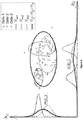
- the curves shown on each axis represent the factorised probability densities for the respective principal component, whereas the ellipses represent bounding parameter values of the SSPDFs, based on both principal components.
- the probability density of all the training data that builds the mixed-subject SSM is denoted by P B g : B g ⁇ ⁇ g , where the reference space ⁇ g is the union of all the subject subspaces.
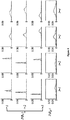
- Figure 4 shows some examples of these factorised probability densities using the histograms of the samples ⁇ b ij ⁇ from the prostate shape data.
- P ( B il ) is different between subjects (i.e. for different values of ( i )), and P ( B il ) is also different from P ( B gl ) , corresponding to the mixed-subject (population) SSM.
- the sample distributions have a generally bell-like shape with different widths and centre positions.
- This PDF is considered as a parametric example of the SSPDF for i th subject, and is entirely characterised by the distribution parameters ⁇ i and ⁇ i 2 .
- the probability distribution associated with a given principal component (as specified by I ) approximates to a Gaussian distribution which can be parameterised by two standard scalar quantities, namely mean ( ⁇ ) and variance ( ⁇ 2 ).
- the optimal regression parameter for a given data set (e.g. for the set of data illustrated in Figure 2 ) may be obtained by using a linear least squares technique to minimise the regularised residual sum-of-squares as follows [14]:
- the kernel parameter h is determined by a cross validation method which is described below.
- the shape parameters b new, 0 for the new subject can be estimated by first non-rigidly registering to the mean shape of the group-wise registration [1], and then projecting onto the principal components of the mixed-subject SSM after removing the rigid component.
- b new ,0 E T s new ,0 ⁇ s ⁇ where s new, 0 is the rigidly-aligned un-deformed shape.
- Each distribution parameter of a new SSPDF can then be computed by taking the conditional expectation of Eq.
- an optimal value is computed by minimising the cross validation error, defined as the root-mean-square of the regression residuals, as in Eq.(5).
- the regression error is computed for each data in a leave-one-out scheme by comparing the difference between the ground-truth distribution parameters, computed from the training data via Eqs.(3) and (4), and the predicted distribution parameters, computed from the test data via Eqs. (6) and (8).
- a golden search strategy was used to then find the optimal value of x within the predefined interval 1 ⁇ x ⁇ 8, with the cross validation error serving as the objective function to minimise.
- a Golden Search also known as a Golden Section Search, represents a standard numerical optimisation algorithm; the theory is described in Kiefer, J. (1953), "Sequential minimax search for a maximum", Proceedings of the American Mathematical Society 4 (3): 502-506, doi:10.2307/2032161 , while an example implementation is described in Press, WH; Teukolsky, SA; Vetterling, WT; Flannery, BP (2007), “Section 10.2. Golden Section Search in One Dimension", Numerical Recipes: The Art of Scientific Computing (3rd ed.), New York: Cambridge University Press, ISBN 978-0-521-88068-8 ).
- One of the advantages of the modelling technique described herein is that it does not require a timing or phase correspondence (such as the position in a breathing cycle) to be established between the motion subspaces. Since only the probability densities are modelled to describe the subject motions, and the motion data can be grouped in an arbitrary order in the training dataset, which overcomes a number of practical difficulties.
- point correspondence still needs to be established between subject subspaces.
- a set of predefined features e.g. anatomical landmarks
- the positions of these features (points) in the image are determined. This then allows the point correspondence to be determined, i.e. for each point or feature, the (corresponding) position of that feature in each image or data set is determined.
- This point correspondence may be estimated, for example, by group-wise surface registration [1].
- inter-subject registration of the training shapes, required to build the mixed-subject SSM was performed using an iterative group-wise registration scheme based on the landmark-guided coherent point drift (LGCPD) method [15], where anatomical apex and base points of the prostate serve as two known corresponding points to assist the registration in finding realistic point correspondence between gland surfaces.
- LGCPD landmark-guided coherent point drift
- each deformed shape was generated by simulating a physical deformation of the reference shape, represented by a FE mesh
- 3D point correspondence between different motion data for each subject is available automatically.
- the inherent correspondence known from FE simulation may be used to establish correspondence within individual subjects, and image-based registrations are used to establish correspondence between different subjects.
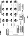
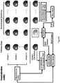
- Figures 5 and 6 illustrate the leave-one-out method for a chosen test subject, where the three linear models are constructed independently.
- the root-mean-square (RMS)-distance-based generalisation ability and specificity then can be computed for each test subject, as per Figures 5 and 6 respectively.
- the cross-validation method described below provides an overall assessment of the modelling ability. Low RMS distance indicates strong generalisation ability and specificity for the linear model.
- the generalisation ability of a linear model quantifies the ability of the model to describe unseen data, and therefore relates closely to a common application of such models, namely capturing organ motion to provide prior information for registering to unseen data.
- the generalisation ability was measured by a separate, embedded leave-one-out scheme [17].
- the generalisation ability was defined as the RMS Euclidean distance between the mesh nodes of an unseen test dataset and the corresponding nodes of the instantiated model fitted to the test data (i.e. the fitted model).
- the unseen test data was the remaining (left-out) data of the 100 biomechanical simulations of the test subject, in the embedded leave-one-out scheme.
- the biomechanically-based SMM was then built independently using the remaining 99 simulations, as illustrated in Fig. 5 .
- the generalisation abilities were computed for the three linear models as mentioned above (subject-specific SMM, biomechanically based SMM, and mixed-subject SSM), all based on the subject-level leave-one-out scheme.
- each linear model For each test subject, one thousand deformed prostate glands for each linear model were generated by randomly sampling b from , and (for each of the three models respectively). The instances generated using each linear model form a set that defines the respective model space. The distance to the nearest training data from the random instance measures the specificity of the linear model.
- Fig. 7 shows example plots of the factorised P ( B il ) for the first four predicted SSPDFs for three new test subjects (solid line - bottom plot), compared with the histogram constructed using the original ⁇ b ij ⁇ (dotted line - top plot). It can be seen that the corresponding curves show excellent agreement between the dotted lines representing P ( B il ) of the data used in this study and the solid lines representing the regression-estimated subject-specific probability density curves for the first four principal components for the three patients. The goodness-of-fit between the corresponding curves was evaluated using the X 2 test. The result - an average p>0.78 - indicates excellent agreement, which provides justification for the effectiveness of the kernel regression analysis and the choice of the Gaussian form to model the PDFs in this study.
- Figure 8 shows examples of random shape instances generated using (i) the biomechanically-based SMM (the ground-truth), (ii) the model-predicted subject-specific SMM of a prostate for the same subject, and (iii) the mixed-subject SSM (which captures the shape variation over the training population of 36 patient prostates). More particularly, the top row of Figure 8 comprises randomly sampled prostate glands from the ground-truth biomechanically-based SMM of a test subject (as in the leave-one-out validation); the middle row comprises randomly selected samples from the model-predicted subject-specific SMM, which are constructed from data excluding the test subject; and the bottom row comprises randomly selected samples from the mixed subject SSM, which includes both intra- and inter-subject shape variations in the training data.
- the first column of Figure 8 shows the reference shape from each model.
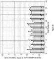
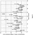
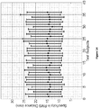
- Figure 9 , Figure 10 and Figure 11 are plots showing the median RMS distance value for the generalisation ability of (i) the model-predicted, subject-specific SMM, (ii) the biomechanical-based, subject-specific SMM generated using the (ground truth) biomechanical simulations, and (iii) the mixed-subject SSM, respectively, for each test subject.
- the error bars indicate the 5th/95th percentiles of these RMS distances. From inspection of these plots, it can be seen that the two subject-specific SMMs provide lower RMS errors (distances) compared with the mixed-subject SSM.
- paired Kolgomorov-Smirnov tests confirm that 1) the mixed-subject SSM has significantly worse generalisation ability than the model-predicted SMM and the biomechanically-based SMM, both with p ⁇ 0.0001 ; and 2) the difference in generalisation ability between the model-predicted SMM and the biomechanically-based SMM is not significantly larger than 0.1mm ( p ⁇ 0.0001 ). Therefore, the proposed model-predicted SMM has a generalisation ability for unseen data which is comparable with that of the original biomechanically-based SMM, while both of these subject-specific models outperform the mixed-subject SSM in this regard (i.e. for generalisation ability).
- Figure 12 , Figure 13 and Figure 14 are plots showing the median RMS distance values of the specificities of the same three linear models, namely (i) the model-predicted subject-specific SMM, (ii) the biomechanical-based subject-specific SMM generated using the (ground truth) biomechanical simulations, and (iii) the mixed-subject SSM, respectively, for each test subject. Again, the error bars indicate the 5th/95th percentiles of these RMS distances. Comparing Figure 12 , Figure 13 and Figure 14 reveals that the subject-specific SMMs provide significantly smaller (better) RMS-distance-based specificities.
- the TRE results using the approach described herein for generating subject-specific SMMs are summarised in Table 1 below, along with published TRE data [12] obtained by registering biomechanically-based subject-specific SMMs. With a confidence level set to 0.05, a paired Kolmogorov-Smirnov test indicates that there is no significant difference between the TREs obtained using these two methods ( p ⁇ 0.0001 ). This suggests that the approach described herein for generating subject-specific SMMs provides a viable (and computationally much easier) alternative to conventional modelling methods that require subject-specific training data without compromising registration accuracy.
- Table 1 Summary of Registration TREs using predicted SSMMs and SMMs Summary Stats Case No.
- This approach described herein provides a new framework for modelling subject-specific organ motion, in which learnt statistics from a training population are used to predict subject-specific training data for an unseen patient, rather than requiring those data to be provided either by dynamic imaging or computer simulation.
- the disclosed method allows subject-specific organ motion to be modelled implicitly, without knowing the explicit motion correspondence between data sets from different individuals.
- the motion modelling method described herein has been compared with biomechanical modelling as a means of generating subject-specific synthetic training data (rather than using dynamic imaging).
- biomechanical simulations One advantage of using biomechanical simulations is that the point correspondences between successive shapes of the organ of a particular subject are known implicitly, since these are computed relative to a common reference shape.
- a significant advantage of the approach described herein is that, since the method is based on modelling SSPDF and kernel regression analysis, only limited subject-specific data on organ shape change during motion is required. Consequently, the method is computationally efficient and highly suited to applications where comprehensive data on organ motion are difficult or impossible to acquire, for example during a surgical intervention.
- the approach disclosed herein is also helpful in situations where imaging is feasible but has significant practical constraints (for example, limited frame rate), meaning that only a small number of training shape instances may be obtained.
- the use of just a single reference shape for unseen subjects overcomes practical constraints that are commonly encountered in the clinical setting, since the reference image can be obtained from diagnostic or planning images, which are widely available in the clinical setting (as in the example provided herein).
- the approach described herein has primarily used subject-specific SMMs to describe the motion of the prostate gland alone, the approach is also applicable to other organs as appropriate, including multi-organ motion. Furthermore, the approach may be easily adapted to use an arbitrary probability function, such as a mixture model if multi-modal distribution is observed, or a different regression technique. Although such adaptations would not result in a straightforward linear model directly, random samples of the subject-specific organ shape could then be drawn from the learnt SSPDF, e.g. via a Monte Carlo approach, and then used to build a linear SMM using standard SSM techniques.
- the approach described herein supports the use of group- and pair-wise landmark-guided coherent point drift (LGCPD) algorithms to non-rigidly register training shapes.
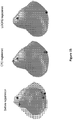
- Figure 15 shows a pair-wise example of such registration, in particular, an example of pair-wise registration of prostate surfaces and anatomical landmarks (apex and base) using the original coherent point drift (CPD) and LGCPD algorithms. It can be seen that the landmarks are better aligned (right) after using the LGCPD algorithm, compared with using the CPD algorithm (middle). Accordingly, the approach described herein provides a faster and more robust extension to general-purpose CPD.
- CPD coherent point drift
- the value of L in Eq. (1) may be chosen so that the reference SSM covers of a certain percentage of the cumulative variance (e.g. at least 99%) in the training data.
- the approach described herein may provide an alternative method to determine an optimal value of L, as components with decreasing variance may contain too much noise to be reasonably modelled by Gaussian or captured by kernel regression.
- multiple subject-specific images are generated using a biomechanical model to deform a single reference image for a given subject.
- the multiple subject-specific images may be acquired via other techniques, including: (i) acquiring a "video" of the subject, i.e. a relatively rapid succession of images frames (2-D or 3-D); or (ii) acquiring multiple (still) images of the subject over a period of time.
- a "video" of the subject i.e. a relatively rapid succession of images frames (2-D or 3-D
- acquiring multiple (still) images of the subject over a period of time e.g. changes in organ shape over time may reflect processes other than motion/deformation (e.g. growth or decay) - it may or may not be beneficial for such processes to be incorporated into the model, depending on the details of the desired application.
- the multiple subject-specific images for any given subject may be acquired from two or more different techniques (such as using both biomechanical modelling and video data), and different techniques (or combinations of techniques) may be used for different subjects.
- a biomechanical model to deform a single reference image for a given subject has the advantage that once the point correspondence has been determined for the reference image, this can then be automatically preserved through the biomechanically modelling for the other images obtained thereby.
- video data once a point correspondence has been determined for one image (image frame) in the video, then it is generally feasible to preserve the point correspondence through difference frames on an automated or semi-automated basis, such as by determining motion vectors from one image frame to the next.
- the approach described herein significantly reduces the time required to build a subject-specific SMM, which is important in many applications, such as modelling prostate motion to enable deformable registration of preoperative MR images to intraoperative TRUS images.
- approach described herein reduces the computational time to both constrain the registration and predict tissue displacements inside the prostate, given surface displacements, from a few hours using a GPU-based FE simulator to a just few seconds without compromising registration accuracy.
- Another potential application of the method disclosed herein is to decompose a conventional SSM using any subject-specific measurements, if available, to provide better modelling ability.
- the model might be used, inter alia, to segment the organ from a second image or to perform an image registration between the second image and the reference image (so that the corresponding positions in the reference and second images for a specific location on or in the organ are determined).
- subject identification such as in the context of facial recognition, where there are multiple subjects, each having a respective reference image, and it is to be determined whether or not a newly acquired image matches one of these reference images (and if so, which one).
- the subject-specific SMM may be used to try to map (register) each reference image to the newly acquired image, and a match is determined for a given reference image if such registration is successful (statistically plausible) within the parameters of the SMM.
- the above embodiments involving various data (signal) processing may be performed by specialised hardware, by general purpose hardware running appropriate computer code, or by some combination of the two.
- the general purpose hardware may comprise a personal computer, a computer workstation, etc.
- the computer code may comprise computer program instructions that are executed by one or more processors to perform the desired operations.
- the one or more processors may be located in or integrated into special purpose apparatus, such as a medical imaging system (MRI, ultrasound, etc).
- the one or more processors may comprise digital signal processors, graphics processing units, central processing units, or any other suitable device.
- the computer program code is generally stored in a non-transitory medium such as an optical disk, flash memory (ROM), or hard drive, and then loaded into random access memory (RAM) prior to access by the one or more processors for execution.
Landscapes
- Engineering & Computer Science (AREA)
- Physics & Mathematics (AREA)
- Theoretical Computer Science (AREA)
- Computer Vision & Pattern Recognition (AREA)
- General Physics & Mathematics (AREA)
- Software Systems (AREA)
- Probability & Statistics with Applications (AREA)
- Computing Systems (AREA)
- General Health & Medical Sciences (AREA)
- Medical Informatics (AREA)
- Evolutionary Computation (AREA)
- Databases & Information Systems (AREA)
- Artificial Intelligence (AREA)
- Multimedia (AREA)
- Health & Medical Sciences (AREA)
- Measuring And Recording Apparatus For Diagnosis (AREA)
- Image Analysis (AREA)
- Ultra Sonic Daignosis Equipment (AREA)
- Image Processing (AREA)
- Magnetic Resonance Imaging Apparatus (AREA)
Description
- The present application relates to a method and apparatus for generating and using a subject-specific statistical motion model, such as may be used in the processing of medical images.
- Statistical shape modelling provides a powerful method to describe and compensate for physical organ shape changes, for example, due to inter-subject anatomical variation, and has been investigated extensively for a range of medical image analysis tasks, including image segmentation [1] and image registration [2]. In particular, the method originally proposed by Cootes et al. [3] in which a low-dimensional, linear statistical shape model (SSM) is constructed by applying principal component analysis (PCA) to image-based shape training data, has been applied to numerous applications where learnt information on organ shape variation provides a useful constraint or prior information. Such models help to ensure that physically implausible organ shapes are not considered, or are at least penalised, when searching for a solution within a segmentation and registration algorithm.
- Variations in the shape of an organ can generally be considered as arising from two sources. The first, termed inter-subject variation, represents differences in organ shape between different people, i.e. from one person to another. Such inter-shape variation naturally arises across a population of individuals. The second, termed intra-subject variation, represents changes in the shape of an organ belonging to one person. Such intra-subject variations can be caused by many different factors, such as a change in posture of the person, natural organ motion (e.g. due to breathing or the beating heart), tissue deformation by the insertion of a medical instrument, the progression or regression of a disease, etc.
- The most common use of SSMs has generally been in describing inter-subject organ shape variation within a population, where intra-subject shape variation is not explicitly considered, and where training data is acquired in a consistent way to try to ensure that the contribution of any intra-patient shape variation is minimised. SSMs that represent intra-subject organ motion may be termed statistical motion models (SMMs) to distinguish them from the more general SSM [6, 7]. One reason for this focus on inter-subject variation is that modelling subject-specific (intra-subject) organ shape variation and organ motion requires sufficient training data from an individual subject to describe statistically the range of shape variation - this is difficult in practice, for example because it may require dynamic imaging data, which may be difficult or impossible to acquire, particularly if the full three-dimensional (3D) variation in organ shape is considered [1]. Particularly challenging examples include modelling non-physiological organ motion due to the intrusion or application of surgical instruments; in such circumstances, it is usually impractical and/or unethical to acquire data on organ shape changes in advance of a surgical procedure.
- One approach to address this problem is to simulate organ motion using biomechanical modelling to provide synthetic training data for building a SSM [4, 5]. However, generating synthetic training data in this way is a complex and potentially time-consuming process that requires segmentation of the organ(s) of interest and computationally-intensive simulations using finite element analysis or an equivalent method. These factors place constraints on the way in which such models may be used for practical applications; for example, SMM generation using this approach is only practical as a pre-operative step in image-guided surgery applications when time is available for performing the necessary image analysis and simulations.
- It is possible to build a population-based SSM using training data that is subject to both inter- and intra-subject organ shape variation, but such models are very likely to perform less effectively or efficiently compared with a subject-specific SMM for approximating subject-specific shape/motion. In particular, such models usually require additional constraints, such as that provided by an elastic model [8], to distinguish between intra- versus inter-subject variation when using the model to instantiate a shape and to prevent the generation of unrealistic or 'over-generalised' shape instances due to inter-subject shape variation.
- The importance of distinguishing inter- and intra-subject shape variation is illustrated by considering the following: if we have first and second organ states, which each corresponds to a different organ shape that arises from intra-subject organ shape variation, then there must be some physical transition of the organ between the first and second states to produce the change in organ shape. A model of such intra-subject variation can be referred to as a SMM (statistical motion model), since the physical transition implies a motion in a general sense (including a shape change due to organ deformation) between the first and second shapes. In contrast, if the differences between the first and second organ shapes arise from inter-subject variation, then they correspond to different individuals, and there is no reason for such a physical transition to exist between the first and second shapes corresponding to some change in state. Accordingly, this type of variation is represented by a more generic SSM (statistic shape model), since the first and second shapes are not generally related to one another by motion.
- If an SSM, based at least in part on inter-subject training data, is used to model subject-specific shape variations, it may permit a variation that is not, in fact, physically plausible for a given organ. As an example, it is generally possible for a human to alter the distance from the eye-line down to the lips (by movement of the lips using facial muscles); however, it is not usually possible to alter the distance or separation between the eyes, since this is determined by the (rigid) skull. On the other hand, the separation between the eyes (in effect, the skull size) does vary from one individual to another. Accordingly, an SSM which is based on at least in part on inter-subject training data might potentially allow variation in this eye separation, despite the fact that such variation is not physically plausible in the context of an individual subject.
- Recently, multilinear analysis [9] has been proposed as a method for dynamic modelling of the heart [10] and cardiac valve [11] motion. This approach enables inter-subject shape variations (e.g., due to subject specific differences in the size and shape of the heart of different individuals) and intra-subject shape variations (e.g. due to physiological heart motion) to be represented by the same statistical model. However, this method requires that inter-subject temporal correspondence between motion subspaces is known - in other words, the states of the organs for different subjects must be correlated, for example, via an independent signal, such as an electrocardiographic (ECG) signal, which measures the electrical activity of the heart and is therefore inherently correlated to its motion. Such an independent signal is very difficult to establish for organs other than the heart and lungs, i.e. for organs where a physiological signal related to motion is not available or very difficult to measure. Furthermore, the cardiac models described in [10, 11] have demonstrated only the ability to predict organ shape at relatively few time-points from the dynamic data available over the remainder of the cardiac cycle.
- In general, subject-specific dynamic data on organ motion, for example, from imaging, is often extremely limited or not available at all, but many examples exist in the context of image-guided surgical procedures where it is desirable to be able provide models which use learnt information on inter- and intra-subject organ shape variation to predict subject-specific organ shape and motion given only sparse and potentially noisy (intraoperative) spatial data that describe the current organ state.
- For example, in a surgical intervention the surgeon may wish to treat or remove a particular anatomical structure or region of diseased tissue which has a specific location determined in advance of the procedure by pre-operative imaging, such as magnetic resonance imaging (MRI). However, this structure or region may be difficult to localise or not be visible using intraoperative imaging, such as ultrasound, during the procedure. Such intraoperative imaging techniques are typically low-cost, portable, and easier to utilise within a surgical procedure, but often do not provide the information of diagnostic-quality pre-operative imaging methods.
- One well-established way of overcoming this difficulty is to perform a (non-rigid) registration (i.e. spatial alignment) between the pre-operative image and the intraoperative image, thereby allowing structures determined in the pre-operative images to be mapped across to (and displayed in conjunction with) the intra-operative images. In practice, this is achieved using special-purpose image fusion software, and an important requirement for surgical applications is that the image registration needs to be performed within a timescale that is acceptable in the context of the surgical procedure. To achieve a high enough accuracy to be of most clinical use, the image registration should also be able to compensate for movement and deformation in the organ or structures of surgical interest, for example, due to changes in the subject position or posture, or as a direct result of instruments used in the surgical procedure itself (for example, organ deformation arising from ultrasound imaging probe pressure). The physical nature of this organ motion in an individual subject suggests that an SMM approach is appropriate, but for cases where dynamic imaging is unavailable, generating a subject-specific SMM by performing biomechanical simulations of organ motion to provide training data is both a complex and time-consuming process, both computationally and from the point of view of implementing within a clinical workflow.
- Yun Zhu et al., "Segmentation of Left Ventricle from 3D cardiac MR image sequences using a subject-specific Dynamical Model", Computer Vision and Pattern Recognition, IEEE conference on, 2008, pages 1-8, discloses a subject-specific dynamical model (SSDM) that handles inter-subject variability and temporal dynamics (intra-subject variability) simultaneously. It can progressively identify the specific motion patterns of a new cardiac sequence based on the segmentations observed in the past frames.
- The invention is defined in the appended claims.
- The approach described herein enables a subject-specific SMM to be built without knowing the correspondence between subject subspaces - in other words, a relationship between the shapes and states of the organs of different subjects does not need to be established. In addition, this approach involves only limited subject-specific geometric data, for example, a reference shape based on the segmentation of one static image, to predict the organ motion for a new (unseen) subject. The application of this approach for deformable registration of MRI and transrectal ultrasound (TRUS) images of the prostate is discussed below.
- More generally, a new framework for statistical shape modelling of subject-specific organ motion, including soft-tissue organ deformation, etc. is described herein. The approach adopted combines modelling of subject-specific probability of shape model parameters with kernel regression analysis to predict organ motion for an unseen subject. The approach is computationally efficient, uses only a limited number of training shape samples for each subject, and is highly suited to image analysis problems where prior subject-specific information on organ shape variation is useful, but where obtaining sufficient training data to construct a statistical shape/motion model for each new subject is impractical or technically or logistically difficult. As an investigation of the approach disclosed herein, subject-specific, MRI-derived statistical prostate motion models are generated and compared with models built using subject-specific training data provided by finite element simulations and mixed subject data that exhibits variation in shape due inter-subject variations and intra-subject prostate motion. The results from this investigation show that the two subject-specific models are generally equivalent in terms of output, and provide much higher specificity than can be obtained with a mixed model built using training datasets from a group of subjects. Furthermore, when used to constrain allowable deformations as part of non-rigid registration algorithm, there was no significant difference in the MRI-to-3D-TRUS target registration error calculated using the two different subject-specific models. These findings indicate that the approach described herein provides a robust, computationally efficient, and practical alternative to subject-specific statistical shape models of organ motion based on simulations, and, potentially, to dynamic imaging.
- Some embodiments of the invention provide a method and an apparatus for building a subject-specific statistical model of shape variation for an anatomical structure using a set of geometric representations of shape for the anatomical structure. Each representation is associated with one of multiple subjects, each subject having a respective subset of associated representations, and each subset comprising multiple representations including a reference representation. The multiple representations correspond to different shapes of the anatomical structure arising from physical motion and/or deformation thereof. The method comprises specifying a set of shape parameters whose values, for any given representation, characterise the shape of the representation, and for each subject, representing a probability distribution of the values of the shape parameters across the subset of representations associated with that subject by a set of subject-specific distribution parameters. The method further comprises determining a regression between the subject-specific distribution parameters and the respective reference representation for each subject, and applying said determined regression to a reference representation for a new subject to determine subject-specific distribution parameters for the new subject. The subject-specific distribution parameters are then used to build a subject-specific statistical motion model for the new subject.
- The geometric representations may, for example, comprise images. The images may be three-dimensional, especially for representing the three-dimensional shape of the anatomical structure. The images may also be two dimensional; this may be appropriate, for example, in a facial recognition systems. The images may be obtained from one or more suitable imaging modalities, such as (without limitation) magnetic resonance imaging (MRI), X-ray computed tomography (CT), positron emission tomography (PET), ultrasound, photo-acoustic imaging (PAT), optical, X-ray or gamma ray imaging, optical microscopy, electron microscopy, etc.
- The geometric representations may also be derived, for example, from biomechanical modelling. Thus the shape of an anatomical structure for a subject might initially be determined by measurement (whether from an image, or by any other appropriate physical measurement technique), and a model fitted to this shape based on known properties of the materials of the anatomical structure, such as elasticity, etc. The model allows the anatomical structure to move or deform in accordance with these known properties, thereby creating other physically realistic shapes for the anatomical structure. Representations of these shapes, in effect, instances of the model corresponding to different locations across the parameter space of the model, can be utilised to provide the geometric representations of shape for the anatomical structure. Such geometric representations can be provided in any appropriate format, for example, as an image generated from the model, or as a set of positions of particular features or landmarks on the anatomical structure according to the configuration of that particular model instance.
- The geometrical representations may be derived from a combination of sources, for example, from multiple different imaging modalities, and/or from biomechanical modelling.
- In some embodiments, the set of shape parameters are determined using principal component analysis (PCA), which provides a compact representation of the domain or space of the geometric representations. However, other embodiments may utilise different shape parameters. For example, if the representations are derived from biomechanical modelling, then the shape parameters might potentially be derived directly from (or correspond to) the values of certain model parameters.
- A wide range of anatomical structures can be modelled using the approach described herein. For example, the anatomical structure may represent an organ, such as the prostate, liver, kidney or heart, comprising soft tissue. Modelling of such organs is typically performed for medical reasons. For example, the modelling may support a non-rigid image registration, which allows a first image to be mapped (registered) to a second image. The first image might be a detailed pre-operative image, such as acquired via MRI, and the second image might be an intra-operative image, such as acquired via ultrasound. The modelling described herein can help the non-rigid image registration to accommodate, in a computationally efficient manner, deformation or motion of the organ, such as may arise from a change in posture of the subject, the presence of a surgical instrument, some change in physiological state, and/or any other source of deformation. The modelling described herein can also be utilised for non-medical purposes, such as facial recognition.
- Various embodiments of the invention will now be described in detail by way of example only with reference to the following drawings:
-
Figure 1 is a schematic overview of the method used to build a subject-specific SMM in accordance with some embodiments of the invention. -
Figure 2 shows a schematic representation of the shapes of the prostates of different subjects. Each shape was generated using biomechanical modelling software to predict the physical deformation under different conditions. -
Figure 3 provides a graphical representation of the factorised probability density P(Bil ) for three different subjects, as determined by a method in accordance with some embodiments of the invention. -
Figure 4 provides a comparison of the factorised probability density for three subjects, compared with for the population as a whole. -
Figures 5 and6 provide a schematic overview of the main leave-one-out method for a chosen test subject, as part of a validation of a method in accordance with some embodiments of the invention. -
Figure 7 compares, for three test subjects, plots obtained using a regression model to provide a predicted subject-specific probability density function (solid line), compared with a histogram constructed using original data samples (dotted line). -
Figure 8 shows examples of random shape instances generated using (i) the ground-truth biomechanically-based SMM, (ii) the model-predicted subject-specific SMM of a prostate for the same subject in accordance with some embodiments of the invention, and (iii) the mixed-subject SSM, which captures the shape variation over the training population of 36 patient prostates. -
Figure 9 ,Figure 10 andFigure 11 are plots showing the median RMS distance values for the generalisation ability of (i) the model-predicted subject-specific SMM in accordance with some embodiments of the invention, (ii) the biomechanical-based subject-specific SMM generated using the (ground truth) biomechanical simulations, and (iii) the mixed-subject SSM, respectively, for each test subject. -
Figure 12 ,Figure 13 andFigure 14 are plots showing the median RMS distance values of the specificities of the three linear models, namely (i) the model-predicted subject-specific SMM in accordance with some embodiments of the invention, (ii) the biomechanical-based subject-specific SMM generated using the (ground truth) biomechanical simulations, and (iii) the mixed-subject SSM, respectively, for each test subject. -
Figure 15 shows a pair-wise example of registration of prostate surfaces and anatomical landmarks. - The approach described herein recognises that variations in organ shape due to motion can be expressed with respect to a 'mixed-subject' (i.e. population-based) SSM built using training data from multiple subjects and multiple shapes for each subject. The resulting SSM captures shape variation both between and within individuals. Kernel regression analysis then provides a method to express the multivariate subject-specific probability density function (SSPDF), which represents the distribution of shape parameters (also known as component scores or weights) related to intra-subject organ motion, as a function of the parameters of a pre-chosen reference shape. Once this relationship has been established, the SSPDF that describes the expected organ motion for a new (i.e. unseen) subject can be estimated from new reference shape data for that subject. The resulting SSPDF can then be used to construct a subject-specific SMM for the new subject.
- A schematic overview of the method used to build a subject-specific SMM is shown in
Figure 1 . The stages involved are as follows: - 1. Build the mixed-subject SSM using all available training data;
- 2. Obtain the shape parameters for each training dataset with respect to the mixed-subject SSM (e.g. by projection for the case of a linear model);
- 3. Estimate the SSPDF for each set of shape parameters corresponding to the different training shapes for each subject. The SSPDF may itself be expressed in parametric form and represented by a number of distribution parameters - e.g. the mean and variance for a Gaussian distribution;
- 4. Identify a reference shape for each subject. For example, the reference shape may describe an organ in its 'resting', un-deformed state, or at a time corresponding to a particular physiological event. The reference shape is then represented by its shape parameters;
- 5. For each subject, perform kernel regression analysis between the parameters that characterise each SSPDF and the shape parameters that specify the reference shape;
- 6. Given the reference shape for a new subject, predict the SSPDF for the new subject using regression analysis;
- 7. Finally, construct a subject-specific SMM for the new subject by using the predicted SSPDF.
- The main steps described above are also illustrated in
Figure 1 . The resulting subject-specific SMM is an alternative to a subject-specific SMM built directly from training data available for this subject (including image-based and simulated training data). Therefore, the subject-specific SMM estimated using this method can be compared directly with one generated using the conventional method. In the following description, an illustration of implementing these steps is provided using the example of building a subject-specific SMM of the prostate that captures deformation caused by the placement of an ultrasound probe in the rectum. -
Figure 2 shows a schematic representation of the shapes of the prostates of I subjects, as represented by triangulated meshes. In this case, the shape of each mesh has been simulated using finite element (FE) modelling to predict various physical deformations of a reference shape in response to the presence of a transrectal ultrasound (TRUS) probe. The 3D position and orientation of the TRUS probe is represented inFigure 2 by a shaded hollow cylinder for each deformed shape instance. - Without assuming an equal number of shapes per subject, varying the pose of a transrectal ultrasound (TRUS) probe and the diameter of the water-filled balloon surrounding the probe in each simulation results in Ji (i = 1,2, ..., I) predicted deformed shapes (for subject i). As described in [5, 12], other unknown parameters, such as tissue elastic properties, may also be included as variables in the simulations to reflect uncertainty in these properties. For each subject, the first shape, denoted by j = 0, is the reference shape and the remaining Ji , i.e. j = 1,2, ...Ji , shapes are deformed instances of the reference shape. In this example, the reference shape represents the prostate in the "resting state", obtained by segmenting a T2-weighted MR image that was acquired without an endorectal coil (or other rectal insertion) in place [12]. The reference shapes are usually normalised to a consistent scale and orientation, so as to provide the most reliable comparability between the different images.
- In general, group-wise surface registration of the meshes can be performed to establish point correspondence between: (i) each deformed shape and the reference shape for each subject, and ii) the reference shapes of different subjects. Where FE simulations are performed to determine the training dataset, the point correspondence between each deformed shape (and the reference shape) is known implicitly. The algorithm used to determine the cross-subject (inter-subject) point correspondence is described below.
- The mixed-subject SSM is constructed by applying principal component analysis (PCA) to


s is the mean shape vector; e l is the eigenvector of the covariance matrix of the (mean-subtracted) training shape vectors corresponding to the lth largest eigenvalue,
s and E as estimates, from the overall data set, of distribution parameters that apply to the whole data set, and which are used to transform the shape properties for a given sample between two different coordinate systems - s g , which represents the coordinate system of the raw image data, and b g , which represents a reduced dimension coordinate system from the PCA. An SSM generated in this way is referred to as the mixed-subject SSM. - The subject-specific probability density for the ith subject is denoted by
 is a multivariate random variable and
 ). Rearranging Eq. (1) we have:

- In Eq, (2), b ij contains the shape parameters of the training data by projecting the coordinates s ij for the jth shape belonging to the ith subject. Note that both s ij and s g are training shape vectors, where the different subscripts just denote differently grouped data.may be simplified by the independence assumption so that this multivariate probability density is expressed as a factorised joint probability density, i.e.,


- (The independence assumption and the multivariate Gaussian assumption, see below, have been discussed extensively in the literature (e.g. see [13]) - however, a more complicated distribution, such as a non-unimodal mixture or a full covariance matrix, may be considered when appropriate. In practice, these assumptions reduce the degrees of freedom of the covariance matrix but maintain the modelling generalisation ability as demonstrated in the cross validation).
- Expressing the probability in this way using the independence assumption enables us to draw an informative plot of the distribution in terms of individual distributions of the scalar random variable Bil for lth shape parameter (corresponding to the lth principal component). An example is shown in
Fig.3 , which provides a graphical representation of the factorised probability density P(Bil ) for three different subjects, labelled asdata 1,data 2 and data 3 (also denoted as Ω i where i=1, 2 or 3) and for two principal components of the mixed-subject SSM (corresponding to the x and y axes). The curves shown on each axis represent the factorised probability densities for the respective principal component, whereas the ellipses represent bounding parameter values of the SSPDFs,based on both principal components. The scalar shape parameters bijl, j = 1,2,...,Ji are Ji samples of the random variable, Bil, as derived from the set of Ji deformed shapes for a given subject (i).
- Similarly, the probability density of all the training data that builds the mixed-subject SSM is denoted by


-
Figure 4 shows some examples of these factorised probability densities using the histograms of the samples {b ij } from the prostate shape data. In particular,Figure 4 presents examples of estimated factorised probability densities P(Bil ), represented by histograms for the prostate shape data, for three different subjects (i=1, 2, 3), while the bottom row represents the corresponding population probability densities P(Bgl ) computed over the entire training data. - Inspecting the plots in
Figure 4 , it is clearly apparent that P(Bil ) is different between subjects (i.e. for different values of (i)), and P(Bil ) is also different from P(Bgl ), corresponding to the mixed-subject (population) SSM. In other words, the population as a whole is used to define the principal components of the data set, but when we then look at the distribution for each principal component, the distributions can be very subject specific. For example, if we consider the distribution for I=1 and 2, it can be seen that the distribution of P(Bil ) is relatively narrow for each subject, whereas the distribution of P(Bgl ) is relatively broad. This may correspond to the example given above of eye separation (albeit that a principal component will generally represent a combination of physical parameters) - in other words, the inter-subject variation for eye separation is relatively broad, but the intra-subject (subject-specific) variation is relatively low. Accordingly, most of the spread in the distribution of P(Bgl ) for I=1 and 2 can be attributed to variations between different individuals, rather than intra-subject variability. In contrast, for I=3 and 4, the distribution of P(Bil ) is relatively broad for each subject. This suggests that intra-subject variability may be an important factor (possibly the most important factor) behind the variability associated with this principal component. - Overall, the approach described herein develops from
Figure 4 a potential mechanism to decompose the whole (population) mixed-subject space into motion- and subject subspaces by modelling the SSPDFs, where the space for (physical) motion corresponds to the intra-subject variation, i.e. transitioning from one physical position of an organ to another physical position in a given subject. - It can also be seen from
Figure 4 that the sample distributions have a generally bell-like shape with different widths and centre positions. Following the independence assumption, the SSPDF may be parameterised by a multivariate Gaussian PDF

vector 

- The distribution parameters for a given subject (i), namely µ i and


- Without loss of generality, we now assume that a (nonlinear) relationship exists between the distribution parameter
 for a given subject (i) and the shape parameters of reference shape b i0 for that same subject. This opens up the possibility of predicting the distribution parameter θ i , and therefore the SSPDF
 , for a new subject (e.g. i=I+1), based solely on the shape parameters of the reference shape for the new subject data and the above relationship.
- In the current study, the distribution parameter is expressed as a linear function of kernels as follows:


Figure 2 ) may be obtained by using a linear least squares technique to minimise the regularised residual sum-of-squares as follows [14]: - First, a regularised estimator


- In practice, the regularisation parameter λ is set to a small constant to avoid over-fitting while maintaining acceptable residuals; λ = 10-8 was used in the investigated presented in this study. The kernel parameter h is determined by a cross validation method which is described below.
- It will be appreciated that although the above analysis is based on kernel regression using Gaussian kernels, any other suitable forms of regression could be used, e.g. non-parametric regression, or using kernels based on higher order polynomials.
- Given reference shape data for a new subject, the shape parameters b new,0 for the new subject can be estimated by first non-rigidly registering to the mean shape of the group-wise registration [1], and then projecting onto the principal components of the mixed-subject SSM after removing the rigid component. Thus:





- Oncehas been estimated, the linear model may be obtained directly by "centering" the predicted diagonal covariance matrix, so that the predicted subject-specific SMM takes the form:


s + Eµ new is equivalent to the mean of the predicted subject-specific SMM and b new represents the new shape parameters. - For each regression kernel parameter, expressed as h = 10 x , an optimal value is computed by minimising the cross validation error, defined as the root-mean-square of the regression residuals, as in Eq.(5). The regression error is computed for each data in a leave-one-out scheme by comparing the difference between the ground-truth distribution parameters, computed from the training data via Eqs.(3) and (4), and the predicted distribution parameters, computed from the test data via Eqs. (6) and (8). In this study, a golden search strategy was used to then find the optimal value of x within the
predefined interval 1 ≤ x ≤ 8, with the cross validation error serving as the objective function to minimise. - (A Golden Search, also known as a Golden Section Search, represents a standard numerical optimisation algorithm; the theory is described in Kiefer, J. (1953), "Sequential minimax search for a maximum", Proceedings of the American Mathematical Society 4 (3): 502-506, doi:10.2307/2032161, while an example implementation is described in Press, WH; Teukolsky, SA; Vetterling, WT; Flannery, BP (2007), "Section 10.2. Golden Section Search in One Dimension", Numerical Recipes: The Art of Scientific Computing (3rd ed.), New York: Cambridge University Press, ISBN 978-0-521-88068-8).
- One of the advantages of the modelling technique described herein is that it does not require a timing or phase correspondence (such as the position in a breathing cycle) to be established between the motion subspaces. Since only the probability densities are modelled to describe the subject motions, and the motion data can be grouped in an arbitrary order in the training dataset, which overcomes a number of practical difficulties. However, point correspondence still needs to be established between subject subspaces. In other words, a set of predefined features (e.g. anatomical landmarks) are specified for an organ (corresponding to the points), and for each image or data set, the positions of these features (points) in the image are determined. This then allows the point correspondence to be determined, i.e. for each point or feature, the (corresponding) position of that feature in each image or data set is determined. This point correspondence may be estimated, for example, by group-wise surface registration [1].
- In one study in accordance with certain embodiments of the present invention, inter-subject registration of the training shapes, required to build the mixed-subject SSM, was performed using an iterative group-wise registration scheme based on the landmark-guided coherent point drift (LGCPD) method [15], where anatomical apex and base points of the prostate serve as two known corresponding points to assist the registration in finding realistic point correspondence between gland surfaces. In this scheme, there is pair-wise registration of every segmentation to the mean shape of the registered segmentations, where the mean shape is updated iteratively until convergence. Typically, this took no more than five iterations. In this example, because each deformed shape was generated by simulating a physical deformation of the reference shape, represented by a FE mesh, 3D point correspondence between different motion data for each subject is available automatically. In other words, the inherent correspondence known from FE simulation may be used to establish correspondence within individual subjects, and image-based registrations are used to establish correspondence between different subjects.
- Finally, the single pair-wise registration using this same method was performed in order to find the point correspondence between the new reference shape data and the mean shape of the group-wise registration.
-
- 1) Data Acquisition - to test the method described above, a subject-specific SMM of an unseen prostate gland was built and compared with an SMM generated directly using biomechanical modelling as described in [12]. The mixed-subject SSM was built using 100 finite-element simulations of TRUS-probe-induced gland deformation for each of 36 patients, leading to 3600 training shapes in total. For each simulation, different probe/balloon positions and orientations, different balloon diameters, and different elastic material properties were applied (further details can be found in [12]. For each of the 36 patients, the reference geometry of the prostate was defined as the shape resulting from a manual segmentation of the capsule in a T2-weighted MR scan (image), performed by an expert clinical observer.
- 2) Cross-validation - a leave-one-out, cross-validation framework was used to assess the generalisation ability and specificity [16, 17] of three linear models: 1) the model-predicted subject-specific SMM, as predicted from the mixed-subject SSM, using the method described herein; 2) a subject-specific SMM, built using the biomechanical simulation data, and 3) a mixed-subject SSM built using a training dataset that represents both inter- and intra-subject organ shape variation (this third model is by definition not subject-specific).
-
Figures 5 and6 illustrate the leave-one-out method for a chosen test subject, where the three linear models are constructed independently. The root-mean-square (RMS)-distance-based generalisation ability and specificity then can be computed for each test subject, as perFigures 5 and6 respectively. The cross-validation method described below provides an overall assessment of the modelling ability. Low RMS distance indicates strong generalisation ability and specificity for the linear model. - The generalisation ability of a linear model, as shown in
Figure 5 , quantifies the ability of the model to describe unseen data, and therefore relates closely to a common application of such models, namely capturing organ motion to provide prior information for registering to unseen data. The generalisation ability was measured by a separate, embedded leave-one-out scheme [17]. The generalisation ability was defined as the RMS Euclidean distance between the mesh nodes of an unseen test dataset and the corresponding nodes of the instantiated model fitted to the test data (i.e. the fitted model). In particular, the RMS-distance-based generalisation ability is given by:
Fig. 5 . The generalisation abilities were computed for the three linear models as mentioned above (subject-specific SMM, biomechanically based SMM, and mixed-subject SSM), all based on the subject-level leave-one-out scheme. - In order to avoid bias, the experiments illustrated in
Figures 5 and6 to validate the linear models adopted a different leave-one-out scheme compared with that used for the estimation of the optimal kernel parameter (as described above). In the validation experiments, each of the 36 model-predicted subject-specific SMMs was tested using a mixed-subject SSM generated from the remaining 35 training datasets. Among these, 34 subjects were used as training data to compute the regression error for the remaining datasets in order to determine the optimal kernel parameter for the regression. - The specificity of each linear model was also computed using the same cross-validation framework, which is similar to the approach adopted in [17]. This measure indicates the degree to which the deformations of a linear model are constrained, which is relevant because it is desirable for the model to be robust to corrupted data, for instance, due to image artefacts or noise. Furthermore, the model should be able to predict missing data. For the purposes of this study, as illustrated in
Fig. 6 , this measure was defined as the RMS distance between each randomly sampled model instance s instance and the nearest data s nearest found in the training data (i.e. the 100 biomechanical simulations), as follows:
- For each test subject, one thousand deformed prostate glands for each linear model were generated by randomly sampling b from,
 and
and (for each of the three models respectively). The instances generated using each linear model form a set that defines the respective model space. The distance to the nearest training data from the random instance measures the specificity of the linear model.
- 3) SMM-based Registration Validation - the approach described herein provides a technique for generating a subject-specific SMM using synthesised training data. The ability of such models to recover actual patient organ motion in real-world applications, such as non-rigid image registration, has been tested. In particular, the accuracy of registering a deformable, model-predicted subject-specific SMM, which is based on MR-derived prostate geometry data, to 3D TRUS images was investigated by quantifying the target registration error (TRE) in the alignment of manually-identified, independent anatomical landmarks for 8 patient datasets following registration using the method described in [12]. The data for these 8 patients was independent of the training data used to build the predictive model. This TRE provides an independent measure of the registration performance that can be compared directly with registrations that make use of SMMs that were built using biomechanical simulations of the prostate motion for each patient.
-
Fig. 7 shows example plots of the factorised P(Bil ) for the first four predicted SSPDFs for three new test subjects (solid line - bottom plot), compared with the histogram constructed using the original {b ij } (dotted line - top plot). It can be seen that the corresponding curves show excellent agreement between the dotted lines representing P(Bil ) of the data used in this study and the solid lines representing the regression-estimated subject-specific probability density curves for the first four principal components for the three patients. The goodness-of-fit between the corresponding curves was evaluated using the X2 test. The result - an average p>0.78 - indicates excellent agreement, which provides justification for the effectiveness of the kernel regression analysis and the choice of the Gaussian form to model the PDFs in this study. -
Figure 8 shows examples of random shape instances generated using (i) the biomechanically-based SMM (the ground-truth), (ii) the model-predicted subject-specific SMM of a prostate for the same subject, and (iii) the mixed-subject SSM (which captures the shape variation over the training population of 36 patient prostates). More particularly, the top row ofFigure 8 comprises randomly sampled prostate glands from the ground-truth biomechanically-based SMM of a test subject (as in the leave-one-out validation); the middle row comprises randomly selected samples from the model-predicted subject-specific SMM, which are constructed from data excluding the test subject; and the bottom row comprises randomly selected samples from the mixed subject SSM, which includes both intra- and inter-subject shape variations in the training data. The first column ofFigure 8 shows the reference shape from each model. - By comparing the general form of the shapes generated using the three methods (see
Figure 8 ), it is visually evident that the subject-specific SMM generates shapes which look more physically realistic than those generated by the mixed-subject SSM, and are closer in appearance to those obtained from the ground-truth biomechanically-based SMM. (It should be noted that because the shape instances shown inFig. 8 are based on random sampling, they are purely illustrative of the form of shapes generated by each SMM, and therefore should be compared groupwise, between rows, and not down each column). -
Figure 9 ,Figure 10 andFigure 11 are plots showing the median RMS distance value for the generalisation ability of (i) the model-predicted, subject-specific SMM, (ii) the biomechanical-based, subject-specific SMM generated using the (ground truth) biomechanical simulations, and (iii) the mixed-subject SSM, respectively, for each test subject. The error bars indicate the 5th/95th percentiles of these RMS distances. From inspection of these plots, it can be seen that the two subject-specific SMMs provide lower RMS errors (distances) compared with the mixed-subject SSM. At a confidence level of 0.05, paired Kolgomorov-Smirnov tests confirm that 1) the mixed-subject SSM has significantly worse generalisation ability than the model-predicted SMM and the biomechanically-based SMM, both with p<0.0001; and 2) the difference in generalisation ability between the model-predicted SMM and the biomechanically-based SMM is not significantly larger than 0.1mm (p<0.0001). Therefore, the proposed model-predicted SMM has a generalisation ability for unseen data which is comparable with that of the original biomechanically-based SMM, while both of these subject-specific models outperform the mixed-subject SSM in this regard (i.e. for generalisation ability). -
Figure 12 ,Figure 13 andFigure 14 are plots showing the median RMS distance values of the specificities of the same three linear models, namely (i) the model-predicted subject-specific SMM, (ii) the biomechanical-based subject-specific SMM generated using the (ground truth) biomechanical simulations, and (iii) the mixed-subject SSM, respectively, for each test subject. Again, the error bars indicate the 5th/95th percentiles of these RMS distances. ComparingFigure 12 ,Figure 13 andFigure 14 reveals that the subject-specific SMMs provide significantly smaller (better) RMS-distance-based specificities. The same paired Kolgomorov-Smirnov statistical test concludes that the difference in specificity between the mixed-subject SSM and either of the other two subject-specific SMMs is significantly larger than 10mm, with p<0.0001. However, the difference between the two subject-specific SMMs is not greater than 1mm (p=0.0005). These results indicate that, compared to the subject-specific SMMs, the ability of the mixed-subject SSM to generate accurate subject-specific data is poor. Furthermore, compared to the biomechanically-based SMM, the proposed model-predicted SMM provides analogous modelling ability in terms of generating subject-specific instances. - The TRE results using the approach described herein for generating subject-specific SMMs are summarised in Table 1 below, along with published TRE data [12] obtained by registering biomechanically-based subject-specific SMMs. With a confidence level set to 0.05, a paired Kolmogorov-Smirnov test indicates that there is no significant difference between the TREs obtained using these two methods (p<0.0001). This suggests that the approach described herein for generating subject-specific SMMs provides a viable (and computationally much easier) alternative to conventional modelling methods that require subject-specific training data without compromising registration accuracy.
Table 1: Summary of Registration TREs using predicted SSMMs and SMMs Summary Stats Case No. 1 2 3 4 5 6 7 8 All Median Start 9.42 (11.39) 14.52 (17.43) 6.29 (9.62) 6.25 (9.42) 9.32 (11.14) 5.86 (8.75) 8.84 (11.65) 6.15 (8.98) 8.13 (15.02) (95% percentile) Model-predicted, subject-specific SMM 2.88 (7.94) 3.95 (10.75) 1.79 (6.86) 1.98 (4.99) 2.81 (7.16) 1.90 (6.09) 2.79 (9.26) 1.92 (5.65) 2.40 (6.19) Biomechanically-based subject-specific SMM 2.68 (7.21) 3.19 (9.62) 1.69 (5.38) 1.56 (5.21) 2.60 (6.84) 1.58 (4.65) 2.92 (7.49) 1.49 (4.66) 2.42 (7.15) - This approach described herein provides a new framework for modelling subject-specific organ motion, in which learnt statistics from a training population are used to predict subject-specific training data for an unseen patient, rather than requiring those data to be provided either by dynamic imaging or computer simulation. The disclosed method allows subject-specific organ motion to be modelled implicitly, without knowing the explicit motion correspondence between data sets from different individuals.
- The motion modelling method described herein has been compared with biomechanical modelling as a means of generating subject-specific synthetic training data (rather than using dynamic imaging). One advantage of using biomechanical simulations is that the point correspondences between successive shapes of the organ of a particular subject are known implicitly, since these are computed relative to a common reference shape. On the other hand, a significant advantage of the approach described herein is that, since the method is based on modelling SSPDF and kernel regression analysis, only limited subject-specific data on organ shape change during motion is required. Consequently, the method is computationally efficient and highly suited to applications where comprehensive data on organ motion are difficult or impossible to acquire, for example during a surgical intervention. Furthermore, the approach disclosed herein is also helpful in situations where imaging is feasible but has significant practical constraints (for example, limited frame rate), meaning that only a small number of training shape instances may be obtained. Moreover, the use of just a single reference shape for unseen subjects overcomes practical constraints that are commonly encountered in the clinical setting, since the reference image can be obtained from diagnostic or planning images, which are widely available in the clinical setting (as in the example provided herein).
- Although the approach described herein has primarily used subject-specific SMMs to describe the motion of the prostate gland alone, the approach is also applicable to other organs as appropriate, including multi-organ motion. Furthermore, the approach may be easily adapted to use an arbitrary probability function, such as a mixture model if multi-modal distribution is observed, or a different regression technique. Although such adaptations would not result in a straightforward linear model directly, random samples of the subject-specific organ shape could then be drawn from the learnt SSPDF, e.g. via a Monte Carlo approach, and then used to build a linear SMM using standard SSM techniques.
- In addition, the approach described herein supports the use of group- and pair-wise landmark-guided coherent point drift (LGCPD) algorithms to non-rigidly register training shapes.
Figure 15 shows a pair-wise example of such registration, in particular, an example of pair-wise registration of prostate surfaces and anatomical landmarks (apex and base) using the original coherent point drift (CPD) and LGCPD algorithms. It can be seen that the landmarks are better aligned (right) after using the LGCPD algorithm, compared with using the CPD algorithm (middle). Accordingly, the approach described herein provides a faster and more robust extension to general-purpose CPD. - (For further information about CPD, please see: Myronenko, A.; Xubo Song, "Point Set Registration: Coherent Point Drift," Pattern Analysis and Machine Intelligence, IEEE Transactions on, vol.32, no.12, pp.2262,2275, Dec. 2010, doi: 10.1109/TPAMI.2010.46; for further information on LGCPD, please see: Hu, Y., Rijkhorst, E. J., Manber, R., Hawkes, D. J., Barratt, D. C. (2010), "Deformable Vessel-Based Registration Using Landmark-Guided Coherent Point Drift". MIAR. (Vol. 6326 pp.60-69). Springer LNCS).
- Referring back to Eq. (1), the value of L in Eq. (1) may be chosen so that the reference SSM covers of a certain percentage of the cumulative variance (e.g. at least 99%) in the training data. The approach described herein may provide an alternative method to determine an optimal value of L, as components with decreasing variance may contain too much noise to be reasonably modelled by Gaussian or captured by kernel regression.
- In the implementations described above, multiple subject-specific images are generated using a biomechanical model to deform a single reference image for a given subject. However, the multiple subject-specific images may be acquired via other techniques, including: (i) acquiring a "video" of the subject, i.e. a relatively rapid succession of images frames (2-D or 3-D); or (ii) acquiring multiple (still) images of the subject over a period of time. Note that with the latter technique, changes in organ shape over time may reflect processes other than motion/deformation (e.g. growth or decay) - it may or may not be beneficial for such processes to be incorporated into the model, depending on the details of the desired application. In addition, the multiple subject-specific images for any given subject may be acquired from two or more different techniques (such as using both biomechanical modelling and video data), and different techniques (or combinations of techniques) may be used for different subjects. As mentioned above, the use of a biomechanical model to deform a single reference image for a given subject has the advantage that once the point correspondence has been determined for the reference image, this can then be automatically preserved through the biomechanically modelling for the other images obtained thereby. Similarly, for video data, once a point correspondence has been determined for one image (image frame) in the video, then it is generally feasible to preserve the point correspondence through difference frames on an automated or semi-automated basis, such as by determining motion vectors from one image frame to the next.
- The approach described herein significantly reduces the time required to build a subject-specific SMM, which is important in many applications, such as modelling prostate motion to enable deformable registration of preoperative MR images to intraoperative TRUS images. In particular, approach described herein reduces the computational time to both constrain the registration and predict tissue displacements inside the prostate, given surface displacements, from a few hours using a GPU-based FE simulator to a just few seconds without compromising registration accuracy. Another potential application of the method disclosed herein is to decompose a conventional SSM using any subject-specific measurements, if available, to provide better modelling ability.
- The approach described herein can be used in many different contexts. For example, given a reference image of an organ for a specific subject (patient), the model might be used, inter alia, to segment the organ from a second image or to perform an image registration between the second image and the reference image (so that the corresponding positions in the reference and second images for a specific location on or in the organ are determined).
- Other potential applications include subject identification, such as in the context of facial recognition, where there are multiple subjects, each having a respective reference image, and it is to be determined whether or not a newly acquired image matches one of these reference images (and if so, which one). In this context, the subject-specific SMM may be used to try to map (register) each reference image to the newly acquired image, and a match is determined for a given reference image if such registration is successful (statistically plausible) within the parameters of the SMM.
- The above embodiments involving various data (signal) processing may be performed by specialised hardware, by general purpose hardware running appropriate computer code, or by some combination of the two. For example, the general purpose hardware may comprise a personal computer, a computer workstation, etc. The computer code may comprise computer program instructions that are executed by one or more processors to perform the desired operations. The one or more processors may be located in or integrated into special purpose apparatus, such as a medical imaging system (MRI, ultrasound, etc). The one or more processors may comprise digital signal processors, graphics processing units, central processing units, or any other suitable device. The computer program code is generally stored in a non-transitory medium such as an optical disk, flash memory (ROM), or hard drive, and then loaded into random access memory (RAM) prior to access by the one or more processors for execution.
- In conclusion, the skilled person will be aware of various modifications that can be made to the above embodiments to reflect the particular circumstances of any given implementation. Moreover, the skilled person will be aware that features from different embodiments can be combined as appropriate in any given implementation. Accordingly, the scope of the present invention is defined by the appended claims and their equivalents.
-
- [1] Heimann, T. & Meinzer, H. P. 2009, "Statistical shape models for 3D medical image segmentation: a review", Med.Image Anal., vol. 13, no. 4, pp. 543-563.
- [2] Barratt, D. C., Chan, C. S. K., Edwards, P. J., Penney, G. P., Slomczykowski, M., Carter, T. J., & Hawkes, D. J. 2008, "Instantiation and registration of statistical shape models of the femur and pelvis using 3D ultrasound imaging", Medical Image Analysis, vol. 12, no. 3, pp. 358-374.
- [3] Cootes, T. F., Taylor, C. J., Cooper, D. H., & Graham, J. 1995, "Active Shape Models - Their Training and Application", Computer Vision and Image Understanding, vol. 61, no. 1, pp. 38-59.
- [4] Mohamed, A., Davatzikos, C., & Taylor, R. 2002, "A Combined Statistical and Biomechanical Model for Estimation of Intra-operative Prostate Deformation," in Medical Image Computing and Computer-Assisted Intervention - MICCAI 2002, LNCS 2489 edn, pp. 452-460.
- [5] Hu, Y., Carter, T., Ahmed, H., Emberton, M., Allen, C., Hawkes, D., & Barratt, D. 2011, "Modelling Prostate Motion for Data Fusion during Image-guided Interventions", Medical Imaging, IEEE Transactions on, vol. 30, no. 11, pp. 1887-1900.
- [6] Hu, Y., Morgan, D., Ahmed, H. U., Pendsé, D., Sahu, M., Allen, C., Emberton, M., & Hawkes, D. &. B. D. 2008b, "A Statistical Motion Model based on Biomechanical Simulations for Data Fusion during Image-guided Prostate Interventions," in MICCAI 2008, LNCS 5241 edn, Springer, pp. 737-744.
- [7] Ehrhardt, J., Werner, R., Schmidt-Richberg A., & Handels, H., 2010, "A statistical shape and motion model for the prediction of respiratory lung motion", SPIE Medical Imaging 2010: Image Processing, vol. 7623, pp. 531-539.
- [8] Wang, Y. & Staib, L. H. 2000, "Physical model-based non-rigid registration incorporating statistical shape information", Medical.Image Analysis., vol. 4, no. 1, pp. 7-20.
- [9] Vasilescu, M.A.O. and Terzopoulos, D., 2002, "Multilinear Analysis of Image Ensembles: TensorFaces." in ECCV2002, Vol. LNCS 2350, pp.447-460.
- [10]Zhu, Y., Papademetris, X., Sinusas, A.J. and Duncan, J.S.: "Bidirectional Segmentation of Three-Dimensional Cardiac MR Images Using a Subject-Specific Dynamical Model." 2008, in MICCAI2008, LNCS 5242, 450-457.
- [11]Grbic, S., lonasec, R., Vitanovski, D., Voigt, I., Wang, Y., Georgescu, B., Navab, N. and Comaniciu, D.: "Complete Valvular Heart Apparatus Model from 4D Cardiac CT." 2006, in MICCAI2010, LNCS 6361, 218-226.
- [12] Hu, Y., Ahmed, H. U., Taylor, Z., Allen, C., Emberton, M., Hawkes, D., & Barratt, D. 2012, "MR to ultrasound registration for image-guided prostate interventions", Medical Image Analysis, vol. 16, no. 3, pp. 687-703.
- [13]Shlens, J. A Tutorial on Principal Component Analysis. 2009. www.snl.salk.edu/~shlens/pca.pdf, Ver. 3.01
- [14]Hastie, T., Tibshirani, R., and Friedman, J., 2009. "The Elements of Statistical Learning: data mining, inference and prediction." 2nd ed., Springer.
- [15]Hu, Y., Rijkhorst, E.-J., Manber, R., Hawkes, D., & Barratt, D. 2010, "Deformable vessel-based registration using landmark-guided coherent point drift," in MIAR'10 Proceedings of the 5th international conference on Medical imaging and augmented reality, vol. 6326 Springer, Beijing, pp. 60-69.
- [16]Styner, M., Rajamani, K., Nolte, L. P., Zsemlye, G., Szekely, G. Ã., Taylor, C., & Davies, R. 2003, "Evaluation of 3D Correspondence Methods for Model Building," pp. 63-75.
- [17]Hu, Y., van den Boom, R., Carter, T., Taylor, Z., Hawkes, D., Ahmed, H. U., Emberton, M., Allen, C., & Barratt, D. 2010, "A comparison of the accuracy of statistical models of prostate motion trained using data from biomechanical simulations", Progress in Biophysics and Molecular Biology, vol. 103, no. 2-3, pp. 262-272.
Claims (15)
- A method for building a subject-specific statistical model of shape variation for an anatomical structure using a set of geometric representations of shape for said anatomical structure, wherein each representation is associated with one of multiple subjects, each subject having a respective subset of associated representations, and each subset comprising multiple representations including a reference representation, said multiple representations corresponding to different shapes of the anatomical structure arising from physical motion and/or deformation thereof, the method comprising specifying a set of shape parameters whose values, for any given representation, characterise the shape of the representation,
the method being characterised by for each subject, representing a probability distribution of the values of the shape parameters across the subset of representations associated with that subject by a set of subject-specific distribution parameters;
determining a regression between the subject-specific distribution parameters and the respective reference representation for each subject;
applying said determined regression to a reference representation for a new subject to determine subject-specific distribution parameters for the new subject; and
using the subject-specific distribution parameters to build a subject-specific statistical motion model, SMM, for the new subject. - The method of claim 1, wherein the set of shape parameters are determined using principal component analysis.
- The method of claim 2, further comprising:providing a set of shape vectors, s g , where g=1, 2,...G, wherein G is the number of representations in said set of representations, such that there is a shape vector corresponding to each representation, and wherein the principal component analysis represents each shape vector by L principal components; andspecifying the set of shape parameters includes building a mixed-subject statistical shape model according to:

s is a mean shape vector; e l is an eigenvector of a covariance matrix of mean-subtracted shape vectors, wherein e l corresponds to an lth largest eigenvalue, collectively describe the gth shape vector; and
optionally wherein the shape vectors, s g , comprise point correspondence data for the set ofrepresentations that track spatial coordinates of a predetermined set of points through variations in shape across the set of representations. - The method of any preceding claim, wherein the probability distribution of values for one of the shape parameters in said set of shape parameters is assumed to be independent of the other shape parameters in said set of shape parameters
- The method of claim 4, wherein there are L shape parameters in said set of shape parameters, and representing the probability distribution () of the values of the shape parameters for the subset of representations associated with a subject (i) is parameterised by a multivariate Gaussian probability density function

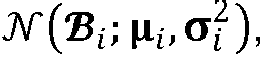


and optionally wherein the distribution parameters for a given subject (i), namely µ i and


- The method of any preceding claim, wherein each distribution parameter is expressed as a linear function of kernels, and/or wherein the regression is determined by a linear least squares technique.
- The method of any preceding claim, wherein specifying a set of shape parameters, whose values for any given representation characterise the shape of the representation, includes building a mixed-subject statistical shape model according to:

s is a mean shape vector; e l is an eigenvector of a covariance matrix of mean-subtracted shape vectors, wherein e l corresponds to an lth largest eigenvalue,
wherein the subject-specific SMM takes the form:
s + Eµ new is equivalent to the mean of the predicted subject-specific SMM, Eµ new being a bias term in which µ new represents a mean value of a distribution parameter as predicted by said regression and b new represents the new shape parameters. - The method of any preceding claim, wherein the anatomical structure comprises an organ formed of soft tissue, and the variations in shape comprise deformation or movement of the organ, and optionally wherein the reference representation describes an organ in its resting or un-deformed state and/or at a time corresponding to a particular physiological event.
- The method of any preceding claim, wherein at least one of the representations comprises an image.
- The method of any preceding claim, wherein at least one of the representations is derived from a biomechanical model.
- The method of any preceding claim, further comprising using anatomical landmarks on said anatomical structure to provide point correspondence data for the set of representations, wherein the point correspondence data are used to track spatial coordinates of a predetermined set of points through variations in shape across the set of representations, and optionally wherein the point correspondence data is determined by performing an image registration between the reference representations for the different subjects.
- The method of any preceding claim, further comprising using the subject-specific statistical motion model for the new subject for one of either image registration or image segmentation, and optionally wherein the image registration or image segmentation is used to support an image-assisted medical intervention.
- A computer program comprising program instructions that when executed by one or more processors of a computer system cause the computer system to perform the steps of the method of any preceding claim.
- A computer program product comprising the computer program of claim 13 stored on a computer readable medium.
- Apparatus adapted to perform the steps of the method of any of claims 1 to 12.
Applications Claiming Priority (2)
| Application Number | Priority Date | Filing Date | Title |
|---|---|---|---|
| GB201403772A GB201403772D0 (en) | 2014-03-04 | 2014-03-04 | Apparatus and method for generating and using a subject-specific statistical motion model |
| PCT/GB2015/050608 WO2015132575A1 (en) | 2014-03-04 | 2015-03-03 | Apparatus and method for generating and using a subject-specific statistical motion model |
Publications (2)
| Publication Number | Publication Date |
|---|---|
| EP3114645A1 EP3114645A1 (en) | 2017-01-11 |
| EP3114645B1 true EP3114645B1 (en) | 2018-11-14 |
Family
ID=50490747
Family Applications (1)
| Application Number | Title | Priority Date | Filing Date |
|---|---|---|---|
| EP15709309.7A Active EP3114645B1 (en) | 2014-03-04 | 2015-03-03 | Apparatus and method for generating and using a subject-specific statistical motion model |
Country Status (7)
| Country | Link |
|---|---|
| US (1) | US10115201B2 (en) |
| EP (1) | EP3114645B1 (en) |
| JP (1) | JP2017512522A (en) |
| AU (1) | AU2015225921A1 (en) |
| CA (1) | CA2940992C (en) |
| GB (1) | GB201403772D0 (en) |
| WO (1) | WO2015132575A1 (en) |
Families Citing this family (13)
| Publication number | Priority date | Publication date | Assignee | Title |
|---|---|---|---|---|
| WO2012096882A1 (en) * | 2011-01-11 | 2012-07-19 | Rutgers, The State University Of New Jersey | Method and apparatus for segmentation and registration of longitudinal images |
| US9851421B2 (en) * | 2015-01-05 | 2017-12-26 | Case Western Reserve University | Differential atlas for cancer assessment |
| US10293184B2 (en) * | 2016-01-29 | 2019-05-21 | Elekta Ltd. | Therapy control using motion prediction |
| JP6821153B2 (en) * | 2016-11-10 | 2021-01-27 | 大日本印刷株式会社 | Living tissue image analysis system, image processing system and program |
| US10952705B2 (en) * | 2018-01-03 | 2021-03-23 | General Electric Company | Method and system for creating and utilizing a patient-specific organ model from ultrasound image data |
| US11631177B2 (en) | 2018-09-13 | 2023-04-18 | Kyoto University | Machine learning device, estimation device, non-transitory computer readable medium, and learned model |
| US10898151B2 (en) * | 2018-10-31 | 2021-01-26 | Medtronic Inc. | Real-time rendering and referencing for medical procedures |
| EP3677186A1 (en) | 2019-01-03 | 2020-07-08 | Siemens Healthcare GmbH | Medical imaging device, system, and method for generating a motion-compensated image, and corresponding storage medium |
| CN111127488B (en) * | 2019-12-29 | 2022-10-14 | 兰州理工大学 | Method for automatically constructing patient anatomical structure model based on statistical shape model |
| US12236517B2 (en) * | 2021-11-16 | 2025-02-25 | Disney Enterprises, Inc. | Techniques for multi-view neural object modeling |
| US12327359B2 (en) * | 2021-11-30 | 2025-06-10 | Shanghai United Imaging Intelligence Co., Ltd. | Image segmentation and tracking based on statistical shape model |
| US12552021B2 (en) * | 2023-03-06 | 2026-02-17 | Nvidia Corporation | Techniques for training and implementing reinforcement learning policies for robot control |
| EP4715738A1 (en) * | 2024-09-18 | 2026-03-25 | Universidade do Minho | Device and method for obtaining a full-surface estimate of an organ from a received partial anatomical point cloud |
Family Cites Families (10)
| Publication number | Priority date | Publication date | Assignee | Title |
|---|---|---|---|---|
| US20070047790A1 (en) * | 2005-08-30 | 2007-03-01 | Agfa-Gevaert N.V. | Method of Segmenting Anatomic Entities in Digital Medical Images |
| US8165359B2 (en) * | 2005-08-30 | 2012-04-24 | Agfa Healthcare N.V. | Method of constructing gray value or geometric models of anatomic entity in medical image |
| GB0521640D0 (en) * | 2005-10-24 | 2005-11-30 | Ccbr As | Automatic quantification of a pathology indicating measure from cartilage scan data |
| US8199985B2 (en) * | 2006-03-24 | 2012-06-12 | Exini Diagnostics Aktiebolag | Automatic interpretation of 3-D medicine images of the brain and methods for producing intermediate results |
| WO2009052497A2 (en) * | 2007-10-18 | 2009-04-23 | The University Of North Carolina At Chapel Hill | Methods, systems, and computer readable media for mapping regions in a model of an object comprising an anatomical structure from one image data set to images used in a diagnostic or therapeutic intervention |
| EP2189942A3 (en) * | 2008-11-25 | 2010-12-15 | Algotec Systems Ltd. | Method and system for registering a medical image |
| GB0913930D0 (en) * | 2009-08-07 | 2009-09-16 | Ucl Business Plc | Apparatus and method for registering two medical images |
| US8724906B2 (en) | 2011-11-18 | 2014-05-13 | Microsoft Corporation | Computing pose and/or shape of modifiable entities |
| JP6000705B2 (en) * | 2012-07-17 | 2016-10-05 | キヤノン株式会社 | Data processing apparatus and data processing method |
| US9269156B2 (en) | 2012-07-24 | 2016-02-23 | Siemens Aktiengesellschaft | Method and system for automatic prostate segmentation in magnetic resonance images |
-
2014
- 2014-03-04 GB GB201403772A patent/GB201403772D0/en not_active Ceased
-
2015
- 2015-03-03 CA CA2940992A patent/CA2940992C/en active Active
- 2015-03-03 AU AU2015225921A patent/AU2015225921A1/en not_active Abandoned
- 2015-03-03 JP JP2016555581A patent/JP2017512522A/en not_active Ceased
- 2015-03-03 US US15/120,991 patent/US10115201B2/en active Active
- 2015-03-03 WO PCT/GB2015/050608 patent/WO2015132575A1/en not_active Ceased
- 2015-03-03 EP EP15709309.7A patent/EP3114645B1/en active Active
Non-Patent Citations (1)
| Title |
|---|
| None * |
Also Published As
| Publication number | Publication date |
|---|---|
| US10115201B2 (en) | 2018-10-30 |
| WO2015132575A1 (en) | 2015-09-11 |
| JP2017512522A (en) | 2017-05-25 |
| GB201403772D0 (en) | 2014-04-16 |
| US20160364880A1 (en) | 2016-12-15 |
| AU2015225921A1 (en) | 2016-09-08 |
| EP3114645A1 (en) | 2017-01-11 |
| CA2940992C (en) | 2022-06-21 |
| CA2940992A1 (en) | 2015-09-11 |
Similar Documents
| Publication | Publication Date | Title |
|---|---|---|
| US10115201B2 (en) | Apparatus and method for generating and using a subject-specific statistical motion model | |
| De Luca et al. | The 2014 liver ultrasound tracking benchmark | |
| Hu et al. | Population-based prediction of subject-specific prostate deformation for MR-to-ultrasound image registration | |
| AU2010280527B2 (en) | Apparatus and method for registering two medical images | |
| CN110770792B (en) | Determining the clinical target volume | |
| US9262583B2 (en) | Image similarity-based finite element model registration | |
| US9761014B2 (en) | System and method for registering pre-operative and intra-operative images using biomechanical model simulations | |
| US20220215625A1 (en) | Image-based methods for estimating a patient-specific reference bone model for a patient with a craniomaxillofacial defect and related systems | |
| Clogenson et al. | A statistical shape model of the human second cervical vertebra | |
| Duchateau et al. | Infarct localization from myocardial deformation: prediction and uncertainty quantification by regression from a low-dimensional space | |
| EP3424017B1 (en) | Automatic detection of an artifact in patient image data | |
| US10977390B2 (en) | Anonymisation of medical patient images using an atlas | |
| US11138736B2 (en) | Information processing apparatus and information processing method | |
| Ruiz‐España et al. | Automatic segmentation of the spine by means of a probabilistic atlas with a special focus on ribs suppression | |
| Vania et al. | Automatic spine segmentation using convolutional neural network via redundant generation of class labels for 3D spine modeling | |
| Hu | Registration of magnetic resonance and ultrasound images for guiding prostate cancer interventions | |
| Pazokifard et al. | Automatic 3D modelling of human diaphragm from lung MDCT images | |
| US11501442B2 (en) | Comparison of a region of interest along a time series of images | |
| Madge | Evaluating Voxelmorph: a learning-based 3D non-linear registration algorithm, against the non-linear symmetric normalization technique from ANTs | |
| Freire et al. | Multiple sclerosis lesion enhancement and white matter region estimation using hyperintensities in FLAIR images | |
| Siciarz et al. | Evaluation of CT to CBCT non-linear dense anatomical block matching registration for prostate patients | |
| Methari et al. | 3D reconstruction of the left atrial geometry from 2D echocardiographic images using deep learning | |
| Boussot et al. | Statistical model for the prediction of lung deformation during video-assisted thoracoscopic surgery | |
| Delmoral et al. | Segmentation of tongue shapes during vowel production in magnetic resonance images based on statistical modelling | |
| Shamsil et al. | A computational model for estimating tumor margins in complementary tactile and 3D ultrasound images |
Legal Events
| Date | Code | Title | Description |
|---|---|---|---|
| STAA | Information on the status of an ep patent application or granted ep patent |
Free format text: STATUS: THE INTERNATIONAL PUBLICATION HAS BEEN MADE |
|
| PUAI | Public reference made under article 153(3) epc to a published international application that has entered the european phase |
Free format text: ORIGINAL CODE: 0009012 |
|
| STAA | Information on the status of an ep patent application or granted ep patent |
Free format text: STATUS: REQUEST FOR EXAMINATION WAS MADE |
|
| 17P | Request for examination filed |
Effective date: 20161004 |
|
| AK | Designated contracting states |
Kind code of ref document: A1 Designated state(s): AL AT BE BG CH CY CZ DE DK EE ES FI FR GB GR HR HU IE IS IT LI LT LU LV MC MK MT NL NO PL PT RO RS SE SI SK SM TR |
|
| AX | Request for extension of the european patent |
Extension state: BA ME |
|
| DAV | Request for validation of the european patent (deleted) | ||
| DAX | Request for extension of the european patent (deleted) | ||
| REG | Reference to a national code |
Ref country code: DE Ref legal event code: R079 Ref document number: 602015019816 Country of ref document: DE Free format text: PREVIOUS MAIN CLASS: G06T0007000000 Ipc: G06T0007120000 |
|
| GRAP | Despatch of communication of intention to grant a patent |
Free format text: ORIGINAL CODE: EPIDOSNIGR1 |
|
| STAA | Information on the status of an ep patent application or granted ep patent |
Free format text: STATUS: GRANT OF PATENT IS INTENDED |
|
| RIC1 | Information provided on ipc code assigned before grant |
Ipc: G06T 7/143 20170101ALI20180514BHEP Ipc: G06T 7/12 20170101AFI20180514BHEP Ipc: G06T 7/149 20170101ALI20180514BHEP |
|
| INTG | Intention to grant announced |
Effective date: 20180605 |
|
| GRAS | Grant fee paid |
Free format text: ORIGINAL CODE: EPIDOSNIGR3 |
|
| GRAA | (expected) grant |
Free format text: ORIGINAL CODE: 0009210 |
|
| STAA | Information on the status of an ep patent application or granted ep patent |
Free format text: STATUS: THE PATENT HAS BEEN GRANTED |
|
| AK | Designated contracting states |
Kind code of ref document: B1 Designated state(s): AL AT BE BG CH CY CZ DE DK EE ES FI FR GB GR HR HU IE IS IT LI LT LU LV MC MK MT NL NO PL PT RO RS SE SI SK SM TR |
|
| REG | Reference to a national code |
Ref country code: CH Ref legal event code: EP Ref country code: AT Ref legal event code: REF Ref document number: 1065747 Country of ref document: AT Kind code of ref document: T Effective date: 20181115 |
|
| REG | Reference to a national code |
Ref country code: DE Ref legal event code: R096 Ref document number: 602015019816 Country of ref document: DE |
|
| REG | Reference to a national code |
Ref country code: IE Ref legal event code: FG4D |
|
| REG | Reference to a national code |
Ref country code: SE Ref legal event code: TRGR |
|
| REG | Reference to a national code |
Ref country code: NL Ref legal event code: MP Effective date: 20181114 |
|
| REG | Reference to a national code |
Ref country code: LT Ref legal event code: MG4D |
|
| REG | Reference to a national code |
Ref country code: AT Ref legal event code: MK05 Ref document number: 1065747 Country of ref document: AT Kind code of ref document: T Effective date: 20181114 |
|
| PG25 | Lapsed in a contracting state [announced via postgrant information from national office to epo] |
Ref country code: AT Free format text: LAPSE BECAUSE OF FAILURE TO SUBMIT A TRANSLATION OF THE DESCRIPTION OR TO PAY THE FEE WITHIN THE PRESCRIBED TIME-LIMIT Effective date: 20181114 Ref country code: LT Free format text: LAPSE BECAUSE OF FAILURE TO SUBMIT A TRANSLATION OF THE DESCRIPTION OR TO PAY THE FEE WITHIN THE PRESCRIBED TIME-LIMIT Effective date: 20181114 Ref country code: HR Free format text: LAPSE BECAUSE OF FAILURE TO SUBMIT A TRANSLATION OF THE DESCRIPTION OR TO PAY THE FEE WITHIN THE PRESCRIBED TIME-LIMIT Effective date: 20181114 Ref country code: LV Free format text: LAPSE BECAUSE OF FAILURE TO SUBMIT A TRANSLATION OF THE DESCRIPTION OR TO PAY THE FEE WITHIN THE PRESCRIBED TIME-LIMIT Effective date: 20181114 Ref country code: NO Free format text: LAPSE BECAUSE OF FAILURE TO SUBMIT A TRANSLATION OF THE DESCRIPTION OR TO PAY THE FEE WITHIN THE PRESCRIBED TIME-LIMIT Effective date: 20190214 Ref country code: ES Free format text: LAPSE BECAUSE OF FAILURE TO SUBMIT A TRANSLATION OF THE DESCRIPTION OR TO PAY THE FEE WITHIN THE PRESCRIBED TIME-LIMIT Effective date: 20181114 Ref country code: BG Free format text: LAPSE BECAUSE OF FAILURE TO SUBMIT A TRANSLATION OF THE DESCRIPTION OR TO PAY THE FEE WITHIN THE PRESCRIBED TIME-LIMIT Effective date: 20190214 Ref country code: IS Free format text: LAPSE BECAUSE OF FAILURE TO SUBMIT A TRANSLATION OF THE DESCRIPTION OR TO PAY THE FEE WITHIN THE PRESCRIBED TIME-LIMIT Effective date: 20190314 Ref country code: FI Free format text: LAPSE BECAUSE OF FAILURE TO SUBMIT A TRANSLATION OF THE DESCRIPTION OR TO PAY THE FEE WITHIN THE PRESCRIBED TIME-LIMIT Effective date: 20181114 |
|
| PG25 | Lapsed in a contracting state [announced via postgrant information from national office to epo] |
Ref country code: GR Free format text: LAPSE BECAUSE OF FAILURE TO SUBMIT A TRANSLATION OF THE DESCRIPTION OR TO PAY THE FEE WITHIN THE PRESCRIBED TIME-LIMIT Effective date: 20190215 Ref country code: RS Free format text: LAPSE BECAUSE OF FAILURE TO SUBMIT A TRANSLATION OF THE DESCRIPTION OR TO PAY THE FEE WITHIN THE PRESCRIBED TIME-LIMIT Effective date: 20181114 Ref country code: AL Free format text: LAPSE BECAUSE OF FAILURE TO SUBMIT A TRANSLATION OF THE DESCRIPTION OR TO PAY THE FEE WITHIN THE PRESCRIBED TIME-LIMIT Effective date: 20181114 Ref country code: PT Free format text: LAPSE BECAUSE OF FAILURE TO SUBMIT A TRANSLATION OF THE DESCRIPTION OR TO PAY THE FEE WITHIN THE PRESCRIBED TIME-LIMIT Effective date: 20190314 Ref country code: NL Free format text: LAPSE BECAUSE OF FAILURE TO SUBMIT A TRANSLATION OF THE DESCRIPTION OR TO PAY THE FEE WITHIN THE PRESCRIBED TIME-LIMIT Effective date: 20181114 |
|
| PG25 | Lapsed in a contracting state [announced via postgrant information from national office to epo] |
Ref country code: PL Free format text: LAPSE BECAUSE OF FAILURE TO SUBMIT A TRANSLATION OF THE DESCRIPTION OR TO PAY THE FEE WITHIN THE PRESCRIBED TIME-LIMIT Effective date: 20181114 Ref country code: IT Free format text: LAPSE BECAUSE OF FAILURE TO SUBMIT A TRANSLATION OF THE DESCRIPTION OR TO PAY THE FEE WITHIN THE PRESCRIBED TIME-LIMIT Effective date: 20181114 Ref country code: DK Free format text: LAPSE BECAUSE OF FAILURE TO SUBMIT A TRANSLATION OF THE DESCRIPTION OR TO PAY THE FEE WITHIN THE PRESCRIBED TIME-LIMIT Effective date: 20181114 Ref country code: CZ Free format text: LAPSE BECAUSE OF FAILURE TO SUBMIT A TRANSLATION OF THE DESCRIPTION OR TO PAY THE FEE WITHIN THE PRESCRIBED TIME-LIMIT Effective date: 20181114 |
|
| REG | Reference to a national code |
Ref country code: DE Ref legal event code: R097 Ref document number: 602015019816 Country of ref document: DE |
|
| PG25 | Lapsed in a contracting state [announced via postgrant information from national office to epo] |
Ref country code: RO Free format text: LAPSE BECAUSE OF FAILURE TO SUBMIT A TRANSLATION OF THE DESCRIPTION OR TO PAY THE FEE WITHIN THE PRESCRIBED TIME-LIMIT Effective date: 20181114 Ref country code: SK Free format text: LAPSE BECAUSE OF FAILURE TO SUBMIT A TRANSLATION OF THE DESCRIPTION OR TO PAY THE FEE WITHIN THE PRESCRIBED TIME-LIMIT Effective date: 20181114 Ref country code: SM Free format text: LAPSE BECAUSE OF FAILURE TO SUBMIT A TRANSLATION OF THE DESCRIPTION OR TO PAY THE FEE WITHIN THE PRESCRIBED TIME-LIMIT Effective date: 20181114 Ref country code: EE Free format text: LAPSE BECAUSE OF FAILURE TO SUBMIT A TRANSLATION OF THE DESCRIPTION OR TO PAY THE FEE WITHIN THE PRESCRIBED TIME-LIMIT Effective date: 20181114 |
|
| PLBE | No opposition filed within time limit |
Free format text: ORIGINAL CODE: 0009261 |
|
| STAA | Information on the status of an ep patent application or granted ep patent |
Free format text: STATUS: NO OPPOSITION FILED WITHIN TIME LIMIT |
|
| 26N | No opposition filed |
Effective date: 20190815 |
|
| REG | Reference to a national code |
Ref country code: SE Ref legal event code: EUG |
|
| PG25 | Lapsed in a contracting state [announced via postgrant information from national office to epo] |
Ref country code: MC Free format text: LAPSE BECAUSE OF FAILURE TO SUBMIT A TRANSLATION OF THE DESCRIPTION OR TO PAY THE FEE WITHIN THE PRESCRIBED TIME-LIMIT Effective date: 20181114 Ref country code: SI Free format text: LAPSE BECAUSE OF FAILURE TO SUBMIT A TRANSLATION OF THE DESCRIPTION OR TO PAY THE FEE WITHIN THE PRESCRIBED TIME-LIMIT Effective date: 20181114 Ref country code: SE Free format text: LAPSE BECAUSE OF NON-PAYMENT OF DUE FEES Effective date: 20190304 |
|
| REG | Reference to a national code |
Ref country code: CH Ref legal event code: PL |
|
| PG25 | Lapsed in a contracting state [announced via postgrant information from national office to epo] |
Ref country code: LU Free format text: LAPSE BECAUSE OF NON-PAYMENT OF DUE FEES Effective date: 20190303 |
|
| REG | Reference to a national code |
Ref country code: BE Ref legal event code: MM Effective date: 20190331 |
|
| PG25 | Lapsed in a contracting state [announced via postgrant information from national office to epo] |
Ref country code: LI Free format text: LAPSE BECAUSE OF NON-PAYMENT OF DUE FEES Effective date: 20190331 Ref country code: CH Free format text: LAPSE BECAUSE OF NON-PAYMENT OF DUE FEES Effective date: 20190331 Ref country code: IE Free format text: LAPSE BECAUSE OF NON-PAYMENT OF DUE FEES Effective date: 20190303 |
|
| PG25 | Lapsed in a contracting state [announced via postgrant information from national office to epo] |
Ref country code: BE Free format text: LAPSE BECAUSE OF NON-PAYMENT OF DUE FEES Effective date: 20190331 Ref country code: FR Free format text: LAPSE BECAUSE OF NON-PAYMENT OF DUE FEES Effective date: 20190331 |
|
| PG25 | Lapsed in a contracting state [announced via postgrant information from national office to epo] |
Ref country code: TR Free format text: LAPSE BECAUSE OF FAILURE TO SUBMIT A TRANSLATION OF THE DESCRIPTION OR TO PAY THE FEE WITHIN THE PRESCRIBED TIME-LIMIT Effective date: 20181114 |
|
| PG25 | Lapsed in a contracting state [announced via postgrant information from national office to epo] |
Ref country code: MT Free format text: LAPSE BECAUSE OF NON-PAYMENT OF DUE FEES Effective date: 20190303 |
|
| PG25 | Lapsed in a contracting state [announced via postgrant information from national office to epo] |
Ref country code: CY Free format text: LAPSE BECAUSE OF FAILURE TO SUBMIT A TRANSLATION OF THE DESCRIPTION OR TO PAY THE FEE WITHIN THE PRESCRIBED TIME-LIMIT Effective date: 20181114 |
|
| PG25 | Lapsed in a contracting state [announced via postgrant information from national office to epo] |
Ref country code: HU Free format text: LAPSE BECAUSE OF FAILURE TO SUBMIT A TRANSLATION OF THE DESCRIPTION OR TO PAY THE FEE WITHIN THE PRESCRIBED TIME-LIMIT; INVALID AB INITIO Effective date: 20150303 |
|
| PG25 | Lapsed in a contracting state [announced via postgrant information from national office to epo] |
Ref country code: MK Free format text: LAPSE BECAUSE OF FAILURE TO SUBMIT A TRANSLATION OF THE DESCRIPTION OR TO PAY THE FEE WITHIN THE PRESCRIBED TIME-LIMIT Effective date: 20181114 |
|
| P01 | Opt-out of the competence of the unified patent court (upc) registered |
Effective date: 20230522 |
|
| PGFP | Annual fee paid to national office [announced via postgrant information from national office to epo] |
Ref country code: GB Payment date: 20260217 Year of fee payment: 12 |
|
| PGFP | Annual fee paid to national office [announced via postgrant information from national office to epo] |
Ref country code: DE Payment date: 20260320 Year of fee payment: 12 |