EP3059695A1 - Constructing and using support vector machines - Google Patents
Constructing and using support vector machines Download PDFInfo
- Publication number
- EP3059695A1 EP3059695A1 EP16155193.2A EP16155193A EP3059695A1 EP 3059695 A1 EP3059695 A1 EP 3059695A1 EP 16155193 A EP16155193 A EP 16155193A EP 3059695 A1 EP3059695 A1 EP 3059695A1
- Authority
- EP
- European Patent Office
- Prior art keywords
- hyperplanes
- samples
- candidate
- hyperplane
- angle
- Prior art date
- Legal status (The legal status is an assumption and is not a legal conclusion. Google has not performed a legal analysis and makes no representation as to the accuracy of the status listed.)
- Granted
Links
Images


Classifications
-
- G—PHYSICS
- G06—COMPUTING OR CALCULATING; COUNTING
- G06N—COMPUTING ARRANGEMENTS BASED ON SPECIFIC COMPUTATIONAL MODELS
- G06N20/00—Machine learning
- G06N20/10—Machine learning using kernel methods, e.g. support vector machines [SVM]
-
- G—PHYSICS
- G06—COMPUTING OR CALCULATING; COUNTING
- G06F—ELECTRIC DIGITAL DATA PROCESSING
- G06F18/00—Pattern recognition
- G06F18/20—Analysing
- G06F18/21—Design or setup of recognition systems or techniques; Extraction of features in feature space; Blind source separation
- G06F18/214—Generating training patterns; Bootstrap methods, e.g. bagging or boosting
-
- G—PHYSICS
- G06—COMPUTING OR CALCULATING; COUNTING
- G06F—ELECTRIC DIGITAL DATA PROCESSING
- G06F18/00—Pattern recognition
- G06F18/20—Analysing
- G06F18/24—Classification techniques
- G06F18/241—Classification techniques relating to the classification model, e.g. parametric or non-parametric approaches
- G06F18/2411—Classification techniques relating to the classification model, e.g. parametric or non-parametric approaches based on the proximity to a decision surface, e.g. support vector machines
-
- G—PHYSICS
- G06—COMPUTING OR CALCULATING; COUNTING
- G06F—ELECTRIC DIGITAL DATA PROCESSING
- G06F18/00—Pattern recognition
- G06F18/20—Analysing
- G06F18/24—Classification techniques
- G06F18/245—Classification techniques relating to the decision surface
- G06F18/2451—Classification techniques relating to the decision surface linear, e.g. hyperplane
-
- G—PHYSICS
- G06—COMPUTING OR CALCULATING; COUNTING
- G06N—COMPUTING ARRANGEMENTS BASED ON SPECIFIC COMPUTATIONAL MODELS
- G06N20/00—Machine learning
-
- G—PHYSICS
- G06—COMPUTING OR CALCULATING; COUNTING
- G06V—IMAGE OR VIDEO RECOGNITION OR UNDERSTANDING
- G06V30/00—Character recognition; Recognising digital ink; Document-oriented image-based pattern recognition
- G06V30/10—Character recognition
- G06V30/19—Recognition using electronic means
- G06V30/191—Design or setup of recognition systems or techniques; Extraction of features in feature space; Clustering techniques; Blind source separation
- G06V30/19173—Classification techniques
Definitions
- the present application generally relates to classifiers and, in particular, to methods and devices that provide computationally-efficient support vector machine learning.
- Support vector machines are used in binary classification of samples.
- a support vector machine is typically constructed using a set of training samples and quadratic programming techniques to solve the difficult computational problem of identifying a suitable classification hyperplane in the relevant data space.
- quadratic programming techniques to solve the difficult computational problem of identifying a suitable classification hyperplane in the relevant data space.
- the building of a support vector machine using indirect quadratic programming is complex and difficult and often is unable to adapt to changes in the set of training samples.
- the present application describes a method of building a support vector machine for classifying a new sample, the support vector machine being based upon a set of samples in an N -dimensional data space, the set of samples having a plurality of samples of one class and a plurality of samples of another class.
- the method includes mapping an angle space to a fixed set of angle vectors and, for each angle vector, finding, for each sample, a candidate hyperplane associated with that angle vector, wherein each candidate hyperplane is a radial distance from an origin point measured along a vector from the origin and normal to the candidate hyperplane, and wherein the vector points to the direction given by the angle vector in the data space.
- the method includes selecting a pair of the candidate hyperplanes as an optimal pair of hyperplanes on the basis of a distance between pairs of the candidate hyperplanes parallel to each other and the number of samples between the candidate hyperplanes; and determining a classification hyperplane as a hyperplane parallel to and between the optimal pair of hyperplanes.
- the classification hyperplane determines whether the new sample is in the one class or in the another class based on which side of the classification hyperplane the new sample is located.
- the present application a support vector machine system for classifying a new sample, the support vector machine being based upon a set of samples in an N -dimensional data space, the set of samples having a plurality of samples of one class and a plurality of samples of another class.
- the system includes one or more processors; memory; and processor-executable instructions that, when executed by the one or more processors cause the one or more processors to carry out one or more of the described methods.
- the method and system are for classifying a portion of an image or video.
- the portion of the image or video defines the new sample in the data space.
- the set of samples are classified image or video data.
- the support vector machine is a classification device.
- the classification device is implemented on a computing device, mobile handheld device, a server, or the like.
- the present application describes non-transitory computer-readable media storing computer-executable program instructions which, when executed, configured a processor to perform the described methods.
- the phrase "at least one of...or" is intended to cover any one or more of the listed elements, including any one of the listed elements alone, any sub-combination, or all of the elements, without necessarily excluding any additional elements, and without necessarily requiring all of the elements.
- Support vector machines are supervised machine learning tools useful in classification and regression analysis.
- SVMs are designed for binary classification. If non-binary classification is required, a common approach is to decompose the problem into a series of binary classification problem. Given a set of training samples, which are either labelled positive "+” or negative "-" (or whatever other binary notation is desired for identifying one class versus another class), a SVM training algorithm intends to find a hyperplane that separates the two classes of training samples with the maximum margin. In one example, the maximum margin is found when the sum of the distance from the hyperplane to the nearest positive sample and the distance from the hyperplane to the nearest negative sample is maximized.
- Figure 1 shows a two-dimensional data space 10.
- the data space may be of n-dimensions in other embodiments and that a hyperplane in an n-dimensional space is a plane of n-1 dimensions (e.g. in a three-dimensional space, the hyperplane is a two-dimensional plane).
- hyperplanes are one-dimensional lines in the data space.
- the data space 10 has six example training samples 12, 14.
- the training samples include samples of one class, here termed “negative” samples 12, and samples of another class, here termed "positive” samples 14.
- Four candidate hyperplanes are shown, labelled H 0 , H 1 , H 2 , H 3 . It will be noted that H 3 does not separate the two classes; H 1 and H 2 do but with smaller margins than Ho; and H 0 separates the two classes with the maximum margin. Accordingly, a good SVM training process will output H 0 as the classification hyperplane, i.e. the hyperplane used to classify new samples as either positive or negative.
- x denotes the sample to be classified
- w the normal vector that defines the desired hyperplane in a SVM
- b is a constant offset, which may be zero in some embodiments.
- ⁇ > denotes the inner product, i.e. the projection of x on to w, which gives a point on w that is a distance from the origin.
- ⁇ ( x i , y i ); 0 ⁇ i ⁇ n ⁇ denote a set of n >1 training samples, where y i ⁇ ⁇ +1, -1 ⁇ denotes the label of x i .
- the function ⁇ is sometimes referred to as the decision function.
- Equation (1) above, b is to be solved as part of the constraint. Equation (1) applies to the case where the training samples are linearly separable. In cases where the samples are not separable or some classification errors are to be allowed for the purpose of avoiding over-training, the SVMs are called soft-margin SVMs, and the following QP problem is formulated and to be solved.
- Equation (2) ⁇ i is a slack variable that allows
- Equation (2) can be further modified by using the so-called kernel trick, i.e., replacing the dot product in Equation (1) and Equation (2) by a kernel K ( ⁇ , ⁇ ). Since K ( ⁇ , ⁇ ) can be interpreted as a dot product in a higher dimensional space, the kernel trick is essentially trying to project the samples into a higher dimensional space where they might become linearly separable.
- K ( ⁇ , ⁇ ) can be interpreted as a dot product in a higher dimensional space
- the kernel trick is essentially trying to project the samples into a higher dimensional space where they might become linearly separable.
- the corresponding QP problem with a kernel K ( ⁇ , ⁇ ) is as follows.
- n is the number of training data samples.
- SVM training algorithm with low computational complexity is desired and may prove critical in real-time applications.
- a desired hyperplane separating the training samples is found directly.
- the processes described below have linear computational complexity O(n), and are also are highly parallelizable.
- the processes described herein are capable of working with dynamic training sets, i.e. sets in which samples are added or removed over time.
- the processes described below are better applicable to situations in which the number of training samples is large and the dimensions of each sample are relatively small.
- the processes below may be suitable for applications like MPEG's Compact Descriptors for Video Analysis (CDVA) that may require online and on-demand training.
- CDVA Compact Descriptors for Video Analysis
- a hyperplane/line separating the samples may be referred to as a classification line or classification hyperplane.
- Each classification line H has two "sibling" lines H - and H+ that are parallel to H and to each other. H - passes through at least one negative sample and H+ passes through at least one positive sample. In this hard margin example, there is no positive or negative sample between H - and H+.
- the classification line may be equidistant between the two sibling lines in some embodiments.
- Figure 2 illustrates the 2D data space 10 with training samples 12, 14.
- the hyperplane/line H 0 is shown with its two sibling lines 16, 18.
- Negative sibling line 16 passes through two negative samples 16 and positive sibling line 18 passes through one positive sample 18.
- x i ( x i, 0 , x i ,1 ) in the 2D space 10.
- ⁇ i,j there is a segment normal to the line 20, denoted ⁇ i,j , that extends to the origin and has an angle ⁇ j .
- the line 20 may be described as the shortest distance between the candidate line and the origin, i.e. the positive length of a vector from the origin and normal to the candidate line.
- the line 20 may be referred to herein as a "radial segment”, “radial distance” or “radius”, in the sense that is the radial length of a segment between the candidate hyperplane and the origin and normal to the candidate hyperplane.
- the angle ⁇ j of the radius may be referred to herein as the "angle vector", the "normal angle” or the "radius angle”.
- FIG. 4 shows the 2D space 10 and the training samples 12, 14.
- the two sibling lines 16, 18 of a classification hyperplane have the same normal angle ⁇ j , but the radius of the "positive" sibling line 18, ⁇ i , j + , is a distance d longer than the radius of the "negative sibling line 16, ⁇ i , j ⁇ , since the two sibling lines are parallel and separated by the distance d.
- the search for an optimal classification hyperplane is carried out as the search for an optimal pair of sibling lines, where the lines are optimal if they maximize d.
- Equations (5) and (6) may be implemented together. For instances, in one example the following process may be used:
- ⁇ j , min ⁇ , ⁇ j , max ⁇ , ⁇ j , min + , and ⁇ j , max + are obtained and updated after each ⁇ i,j is computed.
- the quantization of the angle space is implemented using uniform scalar quantization.
- [0, ⁇ ) may be quantized into ⁇ 0, 0.5236, 1.0472, 1.5708, 2.0944, 2.6180 ⁇ with the step size ⁇ 6 , or ⁇ 0, 0.7854, 1.5708, 2.3562 ⁇ with the step size ⁇ 4 .
- the present application is not limited to these step sizes, or to uniform quantization.
- the complexity of the above-described process is O ( Mn ), mainly due to the complexity of computing ⁇ i,j .
- the possible sibling lines or hyperplanes may be referred to as “candidate lines” or “candidate hyperplanes” herein.
- a pair of “candidate hyperplanes” at the same angle are necessarily parallel to each other and, thus, are sibling lines.
- the pair of candidate hyperplanes at the same angle that result in an optimal distance d and/or number of samples between them (zero or more), may be selected as the optimal pair of candidate hyperplanes that then serve as sibling hyperplanes for defining the classification hyperplane to be used in the SVM.
- FIG. 5 shows, in flowchart form, an example method 100 of building a SVM for classifying a new sample.
- the method 100 includes first quantizing the angle space in operation 102.
- the quantization may be uniform or non-uniform.
- the length of the radius to a candidate hyperplane passing through the sample is determined. From among all the determined radii at angle ⁇ j , the minimum and maximum are found for both positive and negative samples, i.e. ⁇ j , min ⁇ , ⁇ j , max ⁇ , ⁇ j , min + , and ⁇ j , max + , as indicated by operation 106. These maximums and minimums help identify those candidate pairs of hyperplanes that will result in no samples between the pair.
- the radiuses that result in the maximum distance d between pairs of candidate hyperplanes at each angle is found, for example using Equations (5) and (6), above.
- pairs of candidate hyperplanes are selected on the basis that no sample lies between them.
- the identification of the maximum and minimum radii for positive and negative classed samples and the evaluation of Equation (5) ensures that the two sibling hyperplanes at a given candidate angle ⁇ j pass through the two samples of each class that are closest to each other in the radial direction, meaning there are no samples between the planes.
- the angle space is again quantized into an ordered set of candidate angles ⁇ j .
- various sibling hyperplane pairs each a distance d apart may be evaluated in a search to find the pair that has the fewest number of samples between them. Note that each candidate hyperplane does not necessarily need to pass through one of the training samples.
- the hyperplanes passing through the training samples are found and for each class (positive/negative) the hyperplane with the maximum radius and the hyperplane with the minimum radius marks the boundaries of the search space.
- different boundaries may be defined.
- the median radius is one of the boundaries of the search space.
- the search space may be quantized candidate hyperplanes using a radial step size ⁇ .
- the step size 0 ⁇ ⁇ ⁇ d.
- d is an integer multiple of the step size ⁇ ( i.e. ⁇ partitions d).
- the step size ⁇ may be selected to balance speed with computational complexity.
- the step size ⁇ may be constant or may vary based on the angle ⁇ j . In some cases, the step size ⁇ may be varied based on the distance between the minimum radius and maximum radius of the class or whatever other measure is used to determine the boundaries of the search space.
- the above-described process is based on a count of the number of samples "between the pair of hyperplanes", it will be appreciated that the process may be modified to be based upon determining the number of samples on the "wrong" side of their respective hyperplane. That is, count the number of training samples of a class that are supposed to be "below” a hyperplane but are actually “above” the hyperplane, including those that are even beyond the other sibling hyperplane ( i.e. outside the space between the hyerplanes).
- Figure 6 shows, in flowchart form, one example method 200 for building a soft margin SVM for classifying a new sample.
- a distance d between the pairs of hyperplanes is selected.
- the distance d may be selected based upon target application requirements (e.g. desired robustness in classification performance) and/or knowledge about the training data (e.g. statistical variation). Note that as the distance d grows, the trained SVMs become less sensitive to the training samples near the boundary of the decision plane, i.e., the samples in the region between the pairs of hyperplanes.
- index j is initialized to zero. Index j steps through the candidate angles ⁇ j .
- index k is initialized to zero and a length variable l k is initialized to the lower boundary of the search space.
- the length variable is a radius length ⁇ i,j for the candidate sibling hyperplane closest to the origin, and l k +d is the radius length for its sibling.
- the initial length l 0 is set by the boundary of the search space.
- the lower boundary may be the minimum radius ⁇ i,j from among all samples x i . In other embodiments, the lower boundary may be selected in another manner, such as the median radius of one of the classes, an average radius of one of the classes, or some other suitable starting point for the search space.
- the count value that is a minimum is stored as the minimum count C j,min .
- the minimum count and minimum index values are overwritten if a count is determined that is smaller than the currently-stored minimum count.
- the method 200 assesses whether all the angles have been evaluated. If not, then j is incremented in operation 218 and the method 200 returns to operation 206. Otherwise, in operation 220, the optimal sibling hyperplanes are output on the basis that they resulted in the minimum count found across all candidate angles. In operation 222, a classification hyperplane is defined based upon the optimal sibling hyperplanes and in operation 224, that classification hyperplane is used by the SVM in the classification of new samples.
- the distance d between the sibling hyperplanes (or, rather, its inverse) and the number of samples between the sibling hyperplanes (or a count of those samples on the "wrong" side of their hyperplane) may be made variables in a joint cost optimization expression. By finding a minimum joint cost, the optimal d and hyperplanes may be selected.
- each training sample x i is an N -tuple, i.e., has N elements, wherein N is an integer larger than 2.
- the candidate sibling hyperplanes will have the same conditions as were defined above in the 2D case, e.g. they are parallel to each other, one passes through at least one negative sample and the other passes through at least one positive sample, and there are no samples between the hyperplanes.
- the search for optimal sibling hyperplaces is again a search for the candidate sibling hyperplanes that are a maximum distance apart.
- the polar coordinate system is extended to an N -dimensional space (e.g. a spherical coordinate system in a 3D space).
- N -dimensional space e.g. a spherical coordinate system in a 3D space.
- ⁇ e 0 , ... , e N- 1 ⁇ denote an orthonormal basis of the N -dimensional space.
- the hard margin process described above is modified to map the angle space [0, ⁇ ) ⁇ [0,2 ⁇ ) N -2 into an ordered set ⁇ ⁇ 0 , ... , ⁇ M -1 ⁇ . In all remaining operations, the same process is carried out but using ⁇ j for ⁇ j .
- the same extension may be applied to the soft margin process for extending it to higher-dimensional data space.
- hard and soft margin processes may be modified to balance computational complexity and accuracy through various optional refinements or modifications.
- the angle space may be "successively refined".
- the angle space may be "successively refined".
- successively refine that optimal angle vector using finer quantization of a smaller angle space centered around the optimal angle vector.
- the hard margin SVM building process may be modified as follows:
- a hyperplane is uniquely identified by an angle vector ⁇ and a radius ⁇ (the radius being normal to the hyperplane). If the hyperplane is in an N -dimensional space, then the dimensions of ⁇ is N -1.
- the parameter space of ⁇ is quantized and mapped to a finite set. However, in the examples descried above, the parameter ⁇ has not been quantized and can take any positive real value in (0, ⁇ ).
- the processes may map ⁇ into a finite set, e.g. ⁇ r 0 , ... , r L -1 ⁇ .
- the whole parameter space may now be represented by an MxL matrix P , where each entry corresponds to a hyperplane.
- ⁇ ( x i , y i ); 0 ⁇ i ⁇ n ⁇ are the training samples, where each x i is an N -dimensional vector.
- the following operations may be carried out to build a hard margin SVM:
- the training sets are presumed to be static and the static training sets are used to determine a classification hyperplane that is then used to classify new samples.
- the following example processes build upon the above examples involving a quantized parameter space, wherein the matrices P + and P - are used to store the counts of the quantized radii that correspond to hyperplanes through the training samples at the various candidate angle vectors. Because the matrices retain all the calculated counts, the refinement processes need only account for the presence of a new sample or the removal of a sample.
- the search through the matrix for the optimal radius for each angle vector is then carried out for the updated matrix and, if d j has changed, then new sibling hyperplanes are returned.
- the following example process may be used to update the SVM to account for a new sample ( x n , y n ):
- the following example process may be used to update the SVM to account for removal of the sample ( x 0 , y 0 ):
- a training sample is re-classified. For example it may be reclassified from positive to negative.
- a similar approach is used to determine the hyperplane corresponding to each candidate angle vector and to update both the matrices, i.e . increment an element of one matrix and decrement the corresponding element in the other matrix.
- Operation 4 for finding the sibling hyperplanes is then carried out.
- both operations 4(a) and 4(b) are performed since both matrices have been altered by the change.
- Adapting the SVM to account for addition or removal of training samples can also be applied to the case of soft margin SVMs.
- the following examples again presume use of a quantized parameter space and the P matrices.
- To add new sample ( x n , y n ) the following operations may be carried out:
- sample ( x 0 , y 0 ) may be implemented using the following example operations:
- each sample x i remains within one computing unit and thus the bandwidth of moving x i among different computing units is saved.
- each angle ⁇ j remains within one computing unit and thus the subsequent search for ⁇ j , min ⁇ , ⁇ j , max ⁇ , ⁇ j , min + , and ⁇ j , max + is within the computing unit, saving the bandwidth cost of moving ⁇ i,j among different computing units.
- CDVA computer-related software
- Examples include CDVA, medical data analysis and online image classification, voice quality rankings or other user feedback situations.
- CDVA in particular, involves the standardization of descriptors as Compact Descriptors for Video Analysis.
- An analyzer produces a compact representation of a video to be interpreted by a CDVA decoder.
- the application for CDVA may include classification of media and entertainment, for example.
- CDVA may be applied to real-time object classification and identification.
- CDVA may have application to automotive driver assistance or driver-less operation.
- Object classification in images or video is a challenge that may be broken down into binary classification decisions regarding a sample based on a database of training samples.
- CDVA may also benefit from online addition or removal of training samples for refining the classifier.
- a supervised or a semi-supervised system provides training samples as input to train a classifier or a classification engine/machine.
- a training sample can be a matrix of pixels with a class label, or descriptors extracted from such a matrix.
- binary class labels include: representing a human face or not, including a person or not, including a car object or not, representing a finger print or not, including a man-made object or not, etc.
- extracted descriptors include a quantized DCT coefficient matrix, a matrix of quantized color values, SIFT (scale-invariant feature transform) descriptors as described by D. G. Lowe in "Distinctive image features from scale-invariant keypoints", International Journal of Computer Vision, pp. 91-110, 2004 , and their variants, minutiae in biometrics, etc.
- Ongoing training and classification may also be useful for classifiers in real-time or near real-time feedback systems, such as online services in which users can provide positive or negative quality assessments.
- user assessments together with data capturing corresponding system parameters and running status, provide training samples that allow a classifier to be built to help identify important parameters to tune, and/or predict future user experience given a current system status.
- user feedback ranking the call quality may be used to build training samples along with performance data and system parameters like communication bandwidth, signal-to-background noise ratio, echo cancellation settings, speaker phone on/off, packet loss rate, etc.
- FIG. 7 shows, in flowchart form, a generalized process 300 for SVM construction.
- the process 300 includes an operation 302 of finding candidate sibling hyperplane pairs.
- the mechanisms for determining the candidate sibling hyperplane pairs may include defining them along a radius normal to the hyperplanes and at a candidate angle vector to the origin in a coordinate system.
- the angle space is quantized.
- the candidate radii are quantized.
- the search may be based on hard margin or soft margin.
- the optimal candidate sibling hyperplane pair is selected.
- this selection may be on the basis that it maximized the distance between the pair of hyperplanes while ensuring no samples fall between them, i.e. hard margin.
- this selection may be on the basis that it minimizes the number of training samples between the pair of hyperplanes while ensuring that the hyperplanes are at least a minimum distance apart, i.e. soft margin.
- the selection is based on a joint cost optimization expression that attempts to balance the maximization of the distance between the hyperplanes with the minimization of the number of samples between the hyperplanes.
- a classification hyperplane is then determined based upon the optimal sibling hyperplanes.
- the classification hyperplane is parallel to, and equidistant between the two sibling hyperplanes.
- the classification hyperplane is between the two sibling hyperplanes, but not necessarily equidistant between them. For example, if there are more positive (or negative) samples between the optimal sibling hyperplanes, the classification hyperplane may be placed closer to the negative (or positive, respectively) samples, and is thus no longer equidistant between the two sibling hyperplanes.
- the SVM may be updated or refined, without having to run the full construction process, as new training sample data is received, old training samples are removed, or old training samples are reclassified.
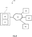
- the system 400 may include a computing device 410 having one or more processors 402 and memory 404.
- the processor(s) 402 execute processor-readable instructions to carry out the operations of the example process for building an SVM.
- the computing device 410 may include a mobile device, such as a smartphone, tablet, laptop, smartwatch, wearable computing device, or any other such mobile computing device.
- the computing device 410 may also include any other type of computing device, including a computer, server, or a special-purpose computing device.
- the system 400 may include one or more remote device 420 configured to communicate with the computing device 410 over one or more wired or wireless networks 430. Any one or more of the operations of a given process may be carried out by one or more of the remote devices 420 and the results provided to the computing device 410.
- the remote devices 420 may include servers, computers, mobile devices, or any other such computing elements.
- the processes and systems according to the present application may be implemented in a number of computing devices, including, without limitation, servers, suitably-programmed general purpose computers, and mobile devices.
- the processes may be implemented by way of software containing instructions for configuring a processor or processors to carry out the functions described herein.
- the software instructions may be stored on any suitable non-transitory computer-readable memory, including CDs, RAM, ROM, Flash memory, etc.
Landscapes
- Engineering & Computer Science (AREA)
- Theoretical Computer Science (AREA)
- Data Mining & Analysis (AREA)
- Computer Vision & Pattern Recognition (AREA)
- Physics & Mathematics (AREA)
- General Physics & Mathematics (AREA)
- Software Systems (AREA)
- Evolutionary Computation (AREA)
- Artificial Intelligence (AREA)
- General Engineering & Computer Science (AREA)
- Bioinformatics & Computational Biology (AREA)
- Evolutionary Biology (AREA)
- Life Sciences & Earth Sciences (AREA)
- Bioinformatics & Cheminformatics (AREA)
- Medical Informatics (AREA)
- Computing Systems (AREA)
- Mathematical Physics (AREA)
- Multimedia (AREA)
- Information Retrieval, Db Structures And Fs Structures Therefor (AREA)
- Image Analysis (AREA)
Abstract
Description
- The present application generally relates to classifiers and, in particular, to methods and devices that provide computationally-efficient support vector machine learning.
- Support vector machines are used in binary classification of samples. A support vector machine is typically constructed using a set of training samples and quadratic programming techniques to solve the difficult computational problem of identifying a suitable classification hyperplane in the relevant data space. With multi-dimensional space, or a large number of samples, the building of a support vector machine using indirect quadratic programming is complex and difficult and often is unable to adapt to changes in the set of training samples.
- Reference will now be made, by way of example, to the accompanying drawings which show example embodiments of the present application, and in which:
-
Figure 1 shows an example 2-dimensional data space with training samples and hyperplanes; -
Figure 2 shows the example data space with sibling hyperplanes; -
Figure 3 shows an example polar coordinate system in the data space; -
Figure 4 shows the data space with a radial distance measurement from origin to hyperplane along a normal vector; -
Figure 5 shows, in flowchart form, one example method of building a support vector machine; -
Figure 6 shows, in flowchart form, another example method of building a support vector machine; -
Figure 7 shows, in flowchart form, yet a further example method of building a support vector machine; and -
Figure 8 shows a block diagram of one embodiment of a system for building and implementing a support vector machine. - Similar reference numerals may have been used in different figures to denote similar components.
- In one aspect, the present application describes a method of building a support vector machine for classifying a new sample, the support vector machine being based upon a set of samples in an N-dimensional data space, the set of samples having a plurality of samples of one class and a plurality of samples of another class. The method includes mapping an angle space to a fixed set of angle vectors and, for each angle vector, finding, for each sample, a candidate hyperplane associated with that angle vector, wherein each candidate hyperplane is a radial distance from an origin point measured along a vector from the origin and normal to the candidate hyperplane, and wherein the vector points to the direction given by the angle vector in the data space. The method includes selecting a pair of the candidate hyperplanes as an optimal pair of hyperplanes on the basis of a distance between pairs of the candidate hyperplanes parallel to each other and the number of samples between the candidate hyperplanes; and determining a classification hyperplane as a hyperplane parallel to and between the optimal pair of hyperplanes. The classification hyperplane determines whether the new sample is in the one class or in the another class based on which side of the classification hyperplane the new sample is located.
- In yet another aspect, the present application a support vector machine system for classifying a new sample, the support vector machine being based upon a set of samples in an N-dimensional data space, the set of samples having a plurality of samples of one class and a plurality of samples of another class. The system includes one or more processors; memory; and processor-executable instructions that, when executed by the one or more processors cause the one or more processors to carry out one or more of the described methods.
- In another aspect, the method and system are for classifying a portion of an image or video. The portion of the image or video defines the new sample in the data space. The set of samples are classified image or video data.
- In another aspect, the support vector machine is a classification device. In some embodiments the classification device is implemented on a computing device, mobile handheld device, a server, or the like.
- In yet a further aspect, the present application describes non-transitory computer-readable media storing computer-executable program instructions which, when executed, configured a processor to perform the described methods.
- Other aspects and features of the present application will be understood by those of ordinary skill in the art from a review of the following description of examples in conjunction with the accompanying figures.
- In the present application, the term "and/or" is intended to cover all possible combination and sub-combinations of the listed elements, including any one of the listed elements alone, any sub-combination, or all of the elements, and without necessarily excluding additional elements.
- In the present application, the phrase "at least one of...or..." is intended to cover any one or more of the listed elements, including any one of the listed elements alone, any sub-combination, or all of the elements, without necessarily excluding any additional elements, and without necessarily requiring all of the elements.
- Support vector machines (SVMs) are supervised machine learning tools useful in classification and regression analysis. In their original forms, SVMs are designed for binary classification. If non-binary classification is required, a common approach is to decompose the problem into a series of binary classification problem. Given a set of training samples, which are either labelled positive "+" or negative "-" (or whatever other binary notation is desired for identifying one class versus another class), a SVM training algorithm intends to find a hyperplane that separates the two classes of training samples with the maximum margin. In one example, the maximum margin is found when the sum of the distance from the hyperplane to the nearest positive sample and the distance from the hyperplane to the nearest negative sample is maximized.
- Reference is now made to
Figure 1 , which shows a two-dimensional data space 10. It will appreciated that the data space may be of n-dimensions in other embodiments and that a hyperplane in an n-dimensional space is a plane of n-1 dimensions (e.g. in a three-dimensional space, the hyperplane is a two-dimensional plane). In the case of a two-dimensional data space, hyperplanes are one-dimensional lines in the data space. - The
data space 10 has sixexample training samples samples 12, and samples of another class, here termed "positive"samples 14. Four candidate hyperplanes are shown, labelled H0, H1, H2, H3. It will be noted that H3 does not separate the two classes; H1 and H2 do but with smaller margins than Ho; and H0 separates the two classes with the maximum margin. Accordingly, a good SVM training process will output H0 as the classification hyperplane, i.e. the hyperplane used to classify new samples as either positive or negative. - Formally, a SVM training algorithm learns the following function from the training samples,

which in turn leads to the following classifier,
- In the above,
x denotes the sample to be classified, w the normal vector that defines the desired hyperplane in a SVM, and b is a constant offset, which may be zero in some embodiments. < > denotes the inner product, i.e. the projection ofx on to w, which gives a point on w that is a distance from the origin. Let {(x i , yi ); 0 ≤ i < n} denote a set of n>1 training samples, where yi ∈ {+1, -1} denotes the label ofx i . The function ƒ is sometimes referred to as the decision function. In order to learn f(x ), typical SVM training algorithms formulate and try to solve the following quadratic programming (QP) problem.
- Note that in Equation (1), above, b is to be solved as part of the constraint. Equation (1) applies to the case where the training samples are linearly separable. In cases where the samples are not separable or some classification errors are to be allowed for the purpose of avoiding over-training, the SVMs are called soft-margin SVMs, and the following QP problem is formulated and to be solved.

- In Equation (2), ξi is a slack variable that allows |f(
x i )| < 1, or even misclassification ofx i ; and C is a constant that weighs the cost of the slackness. The selection of C is often based on heuristics and the target applications. - In cases where non-linear classifiers are needed, Equation (2) can be further modified by using the so-called kernel trick, i.e., replacing the dot product in Equation (1) and Equation (2) by a kernel K(·,·). Since K(·,·) can be interpreted as a dot product in a higher dimensional space, the kernel trick is essentially trying to project the samples into a higher dimensional space where they might become linearly separable. The corresponding QP problem with a kernel K(·,·) is as follows.

- The computational complexity of solving the QP problem can be significant: a brute force implementation has a complexity of O(n3) where n is the number of training data samples. For applications like video analysis where the number n of training samples (e.g. extracted local features) is large, a SVM training algorithm with low computational complexity is desired and may prove critical in real-time applications.
- In accordance with one aspect of the present application, instead of formulating SVM training as a QP problem, a desired hyperplane separating the training samples is found directly. Specifically, the processes described below have linear computational complexity O(n), and are also are highly parallelizable. In some embodiments, the processes described herein are capable of working with dynamic training sets, i.e. sets in which samples are added or removed over time. In some embodiments, the processes described below are better applicable to situations in which the number of training samples is large and the dimensions of each sample are relatively small. The processes below may be suitable for applications like MPEG's Compact Descriptors for Video Analysis (CDVA) that may require online and on-demand training.
- Although some of the example embodiments described below are illustrated using two-dimensional (2D) data spaces or three-dimensional (3D) data spaces, it will be appreciated that the present application is not limited to 2D or 3D data spaces and is generally applicable to an n-dimensional data space.
- Consider the 2D data space with n>1 training samples. Let {(
x i , yi ); 0 ≤ i < n} denote the n training samples, where eachx i is a 2D vector. Note that since the training samples are separable, there exists a line that separates the positive and negative samples. The goal of SVM training is to find the best hyperplane (in this case, a line), i.e. the line that gives the best possible margin in separating positive and negative samples. Since all training samples are classified correctly, these SVMs are called hard-margin SVMs. - Due to the uncertainty about future samples and the linearity of f(
x ), it is not necessary to assume that the solution space for (w , b) is continuous. After all, as long as two candidate solutions (w , b) and (v , c) are sufficiently close, i.e.


x . - A hyperplane/line separating the samples may be referred to as a classification line or classification hyperplane. Each classification line H has two "sibling" lines H- and H+ that are parallel to H and to each other. H- passes through at least one negative sample and H+ passes through at least one positive sample. In this hard margin example, there is no positive or negative sample between H- and H+. In order to select a classification line as the best classification line, one might select the one whose sibling lines have the greatest distance between them. The classification line may be equidistant between the two sibling lines in some embodiments.
-
Figure 2 illustrates the2D data space 10 withtraining samples sibling lines Negative sibling line 16 passes through twonegative samples 16 andpositive sibling line 18 passes through onepositive sample 18. - Reference is now made to
Figure 3 , which shows the2D space 10 with a training samplex i having coordinates (x i,0 , x i,1), i.e.x i = (x i,0, x i,1) in the2D space 10. For every candidate line passing throughx i , there is a segment normal to theline 20, denoted ρi,j, that extends to the origin and has an angle θj . Theline 20 may be described as the shortest distance between the candidate line and the origin, i.e. the positive length of a vector from the origin and normal to the candidate line. Theline 20 may be referred to herein as a "radial segment", "radial distance" or "radius", in the sense that is the radial length of a segment between the candidate hyperplane and the origin and normal to the candidate hyperplane. The angle θj of the radius may be referred to herein as the "angle vector", the "normal angle" or the "radius angle". The radius is given by:
- Reference is now made to
Figure 4 , which shows the2D space 10 and thetraining samples sibling lines sibling line 18,
negative sibling line 16,
- One example process involves quantizing the angle space [0, π) to create an ordered set of candidate angles {θ 0, ..., θ M-1}, where Mis a positive integer. Then, for each
x i , i=0,...,n-1, and for each θj ,j=0,...,M-1, calculate the radius ρi,j . For every candidate angle θj determine

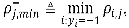


- It will be understood that in a normal training situation, it is not necessarily known whether the "positive" samples will be further from the origin or whether the "negative" samples will be further from the original, so both minimum and maximum radii of both are determined across all samples
x i . The best distance d corresponding to angle θj is then found as:
- From amongst the candidate angles, the optimal one is selected using:

which returns


- In some embodiments, Equations (5) and (6) may be implemented together. For instances, in one example the following process may be used:
- 1. set j=0, compute d 0, and set j* = 0;
- 2. increment j by 1;
- 3. compute dj .
- 4. If dj > dj*, then j* is updated to j; otherwise, nothing needs to be done.
- 5. repeat Steps 2)-4) until j=M-1.
- Similarly, in some embodiments,


- In some embodiments, the quantization of the angle space is implemented using uniform scalar quantization. For example, [0, π) may be quantized into {0, 0.5236, 1.0472, 1.5708, 2.0944, 2.6180} with the step size


- The complexity of the above-described process is O(Mn), mainly due to the complexity of computing ρi,j .
- The possible sibling lines or hyperplanes may be referred to as "candidate lines" or "candidate hyperplanes" herein. A pair of "candidate hyperplanes" at the same angle are necessarily parallel to each other and, thus, are sibling lines. The pair of candidate hyperplanes at the same angle that result in an optimal distance d and/or number of samples between them (zero or more), may be selected as the optimal pair of candidate hyperplanes that then serve as sibling hyperplanes for defining the classification hyperplane to be used in the SVM.
- Reference is now made to
Figure 5 , which shows, in flowchart form, anexample method 100 of building a SVM for classifying a new sample. Themethod 100 includes first quantizing the angle space inoperation 102. As noted above, the quantization may be uniform or non-uniform. - In
operation 104, for each candidate angle θj , and for each samplex i , the length of the radius to a candidate hyperplane passing through the sample is determined. From among all the determined radii at angle θj , the minimum and maximum are found for both positive and negative samples, i.e.


operation 106. These maximums and minimums help identify those candidate pairs of hyperplanes that will result in no samples between the pair. - In
operations - In
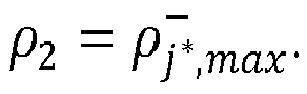
operation 112, the classification hyperplane is then set based upon the optimal angle θ j* and the midpoint between the optimal sibling lines (pair of candidate hyperplanes), i.e.


- It will be noted that the process described above works with any training sets, balanced or unbalanced. Recall that traditional QP-based algorithms find the optimal solution
w * as a weighted sum of training samples, and thus might subject to bias in an unbalanced training set. In the proposed solution, the search for the two best sibling lines is focused on the opposing boundaries of the positive and negative training samples, and thus is not affected by the number of samples behind those boundaries. - In hard margin SVM, pairs of candidate hyperplanes are selected on the basis that no sample lies between them. In the example process outlined above, the identification of the maximum and minimum radii for positive and negative classed samples and the evaluation of Equation (5) ensures that the two sibling hyperplanes at a given candidate angle θj pass through the two samples of each class that are closest to each other in the radial direction, meaning there are no samples between the planes.
- In soft margin SVM, this constraint is relaxed. This can be done to account for classification errors in the training samples that make the samples not linearly separable, and to lower the risk of overtuning. Instead of explicitly introducing the slack variable, as found in Equation (2), the process described below sets a minimum distance d between the sibling hyperplanes and seeks to minimize the number of samples that falls between that pair of hyperplanes.
- In this example process, the angle space is again quantized into an ordered set of candidate angles θj. For each candidate angle θj, various sibling hyperplane pairs each a distance d apart may be evaluated in a search to find the pair that has the fewest number of samples between them. Note that each candidate hyperplane does not necessarily need to pass through one of the training samples.
- In one example embodiment, the hyperplanes passing through the training samples are found and for each class (positive/negative) the hyperplane with the maximum radius and the hyperplane with the minimum radius marks the boundaries of the search space. In other embodiments, different boundaries may be defined. For example, in one embodiment the median radius is one of the boundaries of the search space.
- The search space may be quantized candidate hyperplanes using a radial step size δ. In one example implementation, the
step size 0 < δ < d. In one example, d is an integer multiple of the step size δ (i.e. δ partitions d). For each pair of candidate hyperplanes at angle θj, the number of samples falling between them is counted. Then, the pair with fewest number of samples between them is identified as the optimal pair of candidate hyperplanes for that angle θj. This evaluation is performed for each candidate angle and the angle that produces the pair of hyperplanes with the fewest number of samples between them is selected as the optimal sibling hyperplanes, from which the classification hyperplane is then determined. - The step size δ may be selected to balance speed with computational complexity. The step size δ may be constant or may vary based on the angle θj . In some cases, the step size δ may be varied based on the distance between the minimum radius and maximum radius of the class or whatever other measure is used to determine the boundaries of the search space.
- Although the above-described process is based on a count of the number of samples "between the pair of hyperplanes", it will be appreciated that the process may be modified to be based upon determining the number of samples on the "wrong" side of their respective hyperplane. That is, count the number of training samples of a class that are supposed to be "below" a hyperplane but are actually "above" the hyperplane, including those that are even beyond the other sibling hyperplane (i.e. outside the space between the hyerplanes).
-
Figure 6 shows, in flowchart form, oneexample method 200 for building a soft margin SVM for classifying a new sample. Inoperation 202, a distance d between the pairs of hyperplanes is selected. The distance d may be selected based upon target application requirements (e.g. desired robustness in classification performance) and/or knowledge about the training data (e.g. statistical variation). Note that as the distance d grows, the trained SVMs become less sensitive to the training samples near the boundary of the decision plane, i.e., the samples in the region between the pairs of hyperplanes. - In
operation 204, index j is initialized to zero. Index j steps through the candidate angles θj. Inoperation 206, index k is initialized to zero and a length variable lk is initialized to the lower boundary of the search space. The length variable is a radius length ρi,j for the candidate sibling hyperplane closest to the origin, and lk +d is the radius length for its sibling. The initial length l 0 is set by the boundary of the search space. In one embodiment the lower boundary may be the minimum radius ρi,j from among all samplesx i . In other embodiments, the lower boundary may be selected in another manner, such as the median radius of one of the classes, an average radius of one of the classes, or some other suitable starting point for the search space. - In
operation 208, a count of the number of samples on the "wrong" side of the respective hyperplanes is determined. Because it is not necessarily known which hyperplane corresponds to which class, the count may be determined for both options. In one example, for k=0, the count C is assessed as:

- The count value that is a minimum is stored as the minimum count Cj,min . For k=0, the minimum count may be initialized by storing:

- As indicated by
operation 210, in subsequent iterations, the minimum count and minimum index values are overwritten if a count is determined that is smaller than the currently-stored minimum count. - In
operation 212, themethod 200 evaluates whether the search space is finished. If not, then index k is incremented and radius length / is increased by the step size δ inoperation 214. Subsequent iterations ofoperation 208 may evaluate the expressions:

- Once the search space has been traversed, then in
operation 218 themethod 200 assesses whether all the angles have been evaluated. If not, then j is incremented inoperation 218 and themethod 200 returns tooperation 206. Otherwise, inoperation 220, the optimal sibling hyperplanes are output on the basis that they resulted in the minimum count found across all candidate angles. Inoperation 222, a classification hyperplane is defined based upon the optimal sibling hyperplanes and inoperation 224, that classification hyperplane is used by the SVM in the classification of new samples. - In some embodiments, the computation of


operation 208, is implemented by adding the respective incremental changes to


- In another embodiment, rather than fixing d, the distance d between the sibling hyperplanes (or, rather, its inverse) and the number of samples between the sibling hyperplanes (or a count of those samples on the "wrong" side of their hyperplane) may be made variables in a joint cost optimization expression. By finding a minimum joint cost, the optimal d and hyperplanes may be selected.
- The processes described above in connection with 2D examples may be extended to 3D or higher-dimension data spaces. In a 3D or higher-dimension space, each training sample
x i is an N-tuple, i.e., has N elements, wherein N is an integer larger than 2. - In the case of hard margin SVM, the candidate sibling hyperplanes will have the same conditions as were defined above in the 2D case, e.g. they are parallel to each other, one passes through at least one negative sample and the other passes through at least one positive sample, and there are no samples between the hyperplanes. The search for optimal sibling hyperplaces is again a search for the candidate sibling hyperplanes that are a maximum distance apart.
- The polar coordinate system is extended to an N-dimensional space (e.g. a spherical coordinate system in a 3D space). Specifically, let {
e 0 , ... ,e N-1} denote an orthonormal basis of the N-dimensional space. Then any hyperplane H can be uniquely represented by an N-tuple

- Note that the sum constraint on
θ indicates that the dimension ofθ is N-1. Using a (θ , ρ) representation of a hyperplane, the hard margin process described above is modified to map the angle space [0, π) × [0,2π) N-2 into an ordered set {θ 0, ... ,θ M-1}. In all remaining operations, the same process is carried out but usingθ j forθ j . - The same extension may be applied to the soft margin process for extending it to higher-dimensional data space.
- The above-described hard and soft margin processes may be modified to balance computational complexity and accuracy through various optional refinements or modifications.
- It will be noted that in order to maintain accuracy in mapping the angle space to a discrete set, the set size M grows exponentially with respect to the number N of dimensions. When N is large, M might become too large to be practical. To address this issue, in one embodiment the angle space may be "successively refined". In particular, using the example of hard margin SVMs, first find an optimal angle vector
θ j* and corresponding sibling hyperplanes using a coarse quantization of the angle space. Then successively refine that optimal angle vector using finer quantization of a smaller angle space centered around the optimal angle vector. - For example, the hard margin SVM building process may be modified as follows:
- 1. Initialize a counter τ to 0, and select a positive integer M (0) based on an accuracy level q (0), e.g. a quantization step size. Let V(0) denote the angle space [0, π) × [0,2π) N-2.
- 2. Map V(τ) to an ordered set

θ in V(τ), there is a member in Θ(τ) that is within L1 distance of
θ . - 3. Perform the hard margin SVM building process to determine the optimal angle vector

- 4. Increment τ by 1, and select a new positive integer M (τ) based on a new accuracy level q (τ) < q (τ-1). In one example, q (τ) = αq (τ-1) , where α is a positive constant less than 1. Update V(τ) to be an L1 ball centred at


- 5. Repeat operations 2-4 until desired accuracy is achieved, i.e., q (τ-1) is lower than a prescribed threshold, or the change between


- In one variation of the above embodiment, there might be other angle vectors in Θ(τ) that tie with

- Similar modifications may be made to the soft margin SVM building process to implement successive refinement in that process.
- In the above-described training processes, a hyperplane is uniquely identified by an angle vector
θ and a radius ρ (the radius being normal to the hyperplane). If the hyperplane is in an N-dimensional space, then the dimensions ofθ is N-1. To facilitate the training process, the parameter space ofθ is quantized and mapped to a finite set. However, in the examples descried above, the parameter ρ has not been quantized and can take any positive real value in (0, ∞). In some further embodiments, to simplify the search, the processes may map ρ into a finite set, e.g. {r 0, ... , r L-1}. One consequence of having bothθ and ρ to take values in finite sets is that the whole parameter space may now be represented by an MxL matrix P, where each entry corresponds to a hyperplane. - One example implementation of this quantized parameter space in hard margin SVM construction is described below.
- Suppose that {(
x i , yi ); 0 ≤ i < n} are the training samples, where eachx i is an N-dimensional vector. The following operations may be carried out to build a hard margin SVM: - 1. Map the angle space [0, π) × [0,2π) N-2 in to an ordered set {
θ 0 , ... ,θ M-1}, where M is a positive integer. Initialize two MxL matrices with zeros: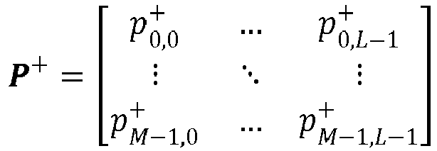

- 2. Let Q denote a mapping from (0, ∞) to an ordered set {r0 , ... , r L-1}, where each rk , 0≤k<L, is a positive real number, and rk < rl for any 0 ≤ k < l < L.
- 3. For each
x i , i=0,...,n-1, and for eachθ j ,j=0,...,M-1, calculate the radius ρi,j of the hyperplane that passesx i and whose angle vector isθ j according to


- 4. For each
θ j :- (a) search from left to right in


- (b) search from left to right in



- (c) compute and store

- (a) search from left to right in
- 5. Determine


- Another example implementation of this quantized parameter space, using soft margin SVM construction in this case, is described below.
- 1. Map the angle space [0, π) × [0,2π) N-2 in to an ordered set {
θ 0, ... ,θ M-1}, where M is a positive integer. Initialize two MxL matrices with zeros:

- 2. Let Q denote a mapping from (0, ∞) to an ordered set {r 0, ... , r L-1}, where each rk , 0≤k<L, is a positive real number, and r k+1 = rk + δ for any 0 ≤ k < L - 1, where δ is a positive constant that divides d.
- 3. For each
x i , i=0,...,n-1, and for eachθ j , j=0,...,M-1, calculate the radius ρi,j of the hyperplane that passesx i and whose angle vector isθ j according to


- 4. For each θj, do the following. For brevity, denote d/δ by t.
- (a) Initialize a counter k=0, and
compute 


- (b) Increment k by 1.
- (c) Update


- (d) Repeat operations (b) and (c) until k ≥ L - 1 - t.
- (a) Initialize a counter k=0, and
- 5. Determine


- In the above examples, the training sets are presumed to be static and the static training sets are used to determine a classification hyperplane that is then used to classify new samples. However, in some applications it may be desirable to allow for dynamic training sets; i.e. to refine or adapt the determination of the classification hyperplane over time as new training samples are generated or old training samples are removed from the set. It would further be advantageous if the refinement/adaptation would avoid re-executing the entire SVM building process each time there is a new training sample or a removed training sample.
- The following example processes build upon the above examples involving a quantized parameter space, wherein the matrices P + and P- are used to store the counts of the quantized radii that correspond to hyperplanes through the training samples at the various candidate angle vectors. Because the matrices retain all the calculated counts, the refinement processes need only account for the presence of a new sample or the removal of a sample.
- For example, in the case of hard margin SVM using a quantized parameter space, a new sample is dealt with by determining the radius of a hyperplane passing through the sample at each of the candidate angle vectors and, for each hyperplane, mapping the radius to the quantized parameter space and incrementing the corresponding matrix value. Note that only one of the matrices is updated since the new training sample is either y = -1 or y = +1. The search through the matrix for the optimal radius for each angle vector is then carried out for the updated matrix and, if dj has changed, then new sibling hyperplanes are returned.
- With reference to the above-described hard margin SVM process with a quantized parameter space, the following example process may be used to update the SVM to account for a new sample (
x n , yn ): - 1. Let i = n.
- 2. For each
θ j , j=0,...,M-1, calculate the radius ρi,j of the hyperplane that passesx i and whose angle vector isθ j according to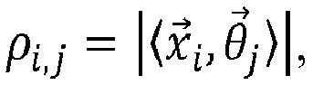


- 3. Perform either operation 4(a) (if yi = -1) or operation 4(b) (if yi = +1) to identify the minimum and maximum radii for both classes, then determine whether the resulting minimum/maximum radii are the same as before or whether they have changed, i.e. is dj the same? If changed, then determine the corresponding sibling hyperplanes as in operation 5, above.
- With reference again to the example hard margin SVM process with a quantized parameter space, the following example process may be used to update the SVM to account for removal of the sample (
x 0, y 0): - 1. Let i = 0.
- 2. For each
θ j ,j=0,...,M-1, calculate the radius ρi,j of the hyperplane that passesx i and whose angle vector isθ j according to


- 3. Perform either operation 4(a) (if yi = -1) or operation 4(b) (if yi = +1) to identify the minimum and maximum radii for both classes, then determine whether the resulting minimum/maximum radii are the same as before or whether they have changed, i.e. is dj the same? If changed, then determine the corresponding sibling hyperplanes as in operation 5, above.
- Yet another situation is that a training sample is re-classified. For example it may be reclassified from positive to negative. In such a case, a similar approach is used to determine the hyperplane corresponding to each candidate angle vector and to update both the matrices, i.e. increment an element of one matrix and decrement the corresponding element in the other matrix. Operation 4 for finding the sibling hyperplanes is then carried out. In the case of a re-classified training sample, both operations 4(a) and 4(b) are performed since both matrices have been altered by the change.
- Adapting the SVM to account for addition or removal of training samples can also be applied to the case of soft margin SVMs. The following examples again presume use of a quantized parameter space and the P matrices. To add new sample (
x n , yn ) the following operations may be carried out: - 1. Let i = n.
- 2. For each
θ j , j=0,...,M-1, calculate the radius ρi,j of the hyperplane that passesx i and whose angle vector isθ j according to


- 3. Perform operations 4 and 5 to update the SVM.
- The removal of sample (
x 0, y 0) may be implemented using the following example operations: - 1. Let i = 0.
- 2. For each
θ j , j=0,...,M-1, calculate the radius ρi,j of the hyperplane that passesx i and whose angle vector isθ j according to


- 3. Perform operations 4 and 5 to update the SVM.
- Reclassification of an existing sample involves the following operation:
- For each
θ j, j=0,...,M-1, calculate the radius ρi,j of the hyperplane that passesx i and whose angle vector isθ j according to


- In general, the above-described processes lend themselves to parallel implementation. For example, in the case of the hard margin SVM first described above, the computation of ρi,j for (
x i , θj ) is independent of any other ρi',j' where (i,j) ≠ (i',j'), which indicates that L>1 computing units may be used to compute L different ρi,j simultaneously. - In one example embodiment, L computing units are used where the ith unit is used to compute {ρi,j ; j = 0, ... , M - 1} for
x i ,x i+L ,x i+2L ,.... In this case, each samplex i remains within one computing unit and thus the bandwidth of movingx i among different computing units is saved. - In another example embodiment, L computing units are used where the jth unit is used to compute {ρi,j ; i = 0, ... , n - 1} for
θ j,θ j+ L,θ j+2L , .... In this case, each angleθ j remains within one computing unit and thus the subsequent search for


- The above-described example processes for building and/or modifying an SVM may be applied to a number of classification problems. Examples include CDVA, medical data analysis and online image classification, voice quality rankings or other user feedback situations. CDVA, in particular, involves the standardization of descriptors as Compact Descriptors for Video Analysis. An analyzer produces a compact representation of a video to be interpreted by a CDVA decoder. The application for CDVA may include classification of media and entertainment, for example. In some cases, CDVA may be applied to real-time object classification and identification. CDVA may have application to automotive driver assistance or driver-less operation. Object classification in images or video is a challenge that may be broken down into binary classification decisions regarding a sample based on a database of training samples. CDVA may also benefit from online addition or removal of training samples for refining the classifier.
- In the context of classifying objects in image and video data, a supervised or a semi-supervised system provides training samples as input to train a classifier or a classification engine/machine. A training sample can be a matrix of pixels with a class label, or descriptors extracted from such a matrix. Typical examples of binary class labels include: representing a human face or not, including a person or not, including a car object or not, representing a finger print or not, including a man-made object or not, etc. Typical examples of extracted descriptors include a quantized DCT coefficient matrix, a matrix of quantized color values, SIFT (scale-invariant feature transform) descriptors as described by D. G. Lowe in "Distinctive image features from scale-invariant keypoints", International Journal of Computer Vision, pp. 91-110, 2004, and their variants, minutiae in biometrics, etc.
- Ongoing training and classification may also be useful for classifiers in real-time or near real-time feedback systems, such as online services in which users can provide positive or negative quality assessments. Such user assessments, together with data capturing corresponding system parameters and running status, provide training samples that allow a classifier to be built to help identify important parameters to tune, and/or predict future user experience given a current system status. For example, in a typical voice over IP (internet protocol) application, user feedback ranking the call quality may be used to build training samples along with performance data and system parameters like communication bandwidth, signal-to-background noise ratio, echo cancellation settings, speaker phone on/off, packet loss rate, etc.
- Other applications will be appreciated by those skilled in the art.
- Reference is made to
Figure 7 , which shows, in flowchart form, ageneralized process 300 for SVM construction. Theprocess 300 includes anoperation 302 of finding candidate sibling hyperplane pairs. As noted in the above examples, the mechanisms for determining the candidate sibling hyperplane pairs may include defining them along a radius normal to the hyperplanes and at a candidate angle vector to the origin in a coordinate system. In some cases, the angle space is quantized. In some cases, the candidate radii are quantized. The search may be based on hard margin or soft margin. - In
operation 304, the optimal candidate sibling hyperplane pair is selected. In one embodiment, this selection may be on the basis that it maximized the distance between the pair of hyperplanes while ensuring no samples fall between them, i.e. hard margin. In another embodiment, this selection may be on the basis that it minimizes the number of training samples between the pair of hyperplanes while ensuring that the hyperplanes are at least a minimum distance apart, i.e. soft margin. In yet another embodiment, the selection is based on a joint cost optimization expression that attempts to balance the maximization of the distance between the hyperplanes with the minimization of the number of samples between the hyperplanes. - In
operation 306, having selected the optimal sibling hyperplanes, a classification hyperplane is then determined based upon the optimal sibling hyperplanes. In one embodiment, the classification hyperplane is parallel to, and equidistant between the two sibling hyperplanes. In another embodiment, the classification hyperplane is between the two sibling hyperplanes, but not necessarily equidistant between them. For example, if there are more positive (or negative) samples between the optimal sibling hyperplanes, the classification hyperplane may be placed closer to the negative (or positive, respectively) samples, and is thus no longer equidistant between the two sibling hyperplanes. - In
operation 308, new samples are classified using the classification hyperplane. - It will further be understood that the SVM may be updated or refined, without having to run the full construction process, as new training sample data is received, old training samples are removed, or old training samples are reclassified.
- Reference is now also made to
Figure 8 , which shows, in block diagram form, oneexample system 400 for implementation of one of the above-described example processes. Thesystem 400 may include acomputing device 410 having one ormore processors 402 andmemory 404. The processor(s) 402 execute processor-readable instructions to carry out the operations of the example process for building an SVM. Thecomputing device 410 may include a mobile device, such as a smartphone, tablet, laptop, smartwatch, wearable computing device, or any other such mobile computing device. Thecomputing device 410 may also include any other type of computing device, including a computer, server, or a special-purpose computing device. - In some cases, the
system 400 may include one or moreremote device 420 configured to communicate with thecomputing device 410 over one or more wired orwireless networks 430. Any one or more of the operations of a given process may be carried out by one or more of theremote devices 420 and the results provided to thecomputing device 410. Theremote devices 420 may include servers, computers, mobile devices, or any other such computing elements. - It will be appreciated that the processes and systems according to the present application may be implemented in a number of computing devices, including, without limitation, servers, suitably-programmed general purpose computers, and mobile devices. The processes may be implemented by way of software containing instructions for configuring a processor or processors to carry out the functions described herein. The software instructions may be stored on any suitable non-transitory computer-readable memory, including CDs, RAM, ROM, Flash memory, etc.
- It will be understood that the devices described herein and the module, routine, process, thread, or other software components implementing the described methods/processes may be realized using standard computer programming techniques and languages. The present application is not limited to particular processors, computer languages, computer programming conventions, data structures, other such implementation details. Those skilled in the art will recognize that the described processes may be implemented as a part of computer-executable code stored in volatile or non-volatile memory, as part of an application-specific integrated chip (ASIC), etc.
- Certain adaptations and modifications of the described embodiments can be made. Therefore, the above discussed embodiments are considered to be illustrative and not restrictive.
Claims (15)
- A method of classifying a portion of an image or video using a classifier, the classifier being based upon a set of samples in a data space, wherein each sample of the set of samples comprises classified image data, wherein the set includes a plurality of samples of one class and a plurality of samples of another class, and wherein the portion of the image or video comprises a new sample in the data space, the method comprising:training the classifier by:mapping an angle space to a fixed set of angle vectors and, for each angle vector,finding, for each sample, a candidate hyperplane associated with that angle vector, wherein each candidate hyperplane is a radial distance from an origin point measured along a vector from the origin and normal to the candidate hyperplane, and wherein the direction of the vector is given by the angle vector in the data space;selecting, as an optimal pair of hyperplanes, a pair of the candidate hyperplanes associated with one angle vector of the first set of angle vectors on the basis of a distance between pairs of the candidate hyperplanes parallel to each other and the number of samples between the candidate hyperplanes; anddetermining a classification hyperplane as a hyperplane parallel to and between the optimal pair of hyperplanes, anddetermining whether the portion of the image or video is in the one class or in the another class based on which side of the classification hyperplane the new sample is located.
- The method claimed in claim 1, wherein, each candidate hyperplane passes through at least one of the samples of one of the classes, and wherein selecting comprises selecting the optimal pair of hyperplanes on the basis that they have the largest distance between them among all pairs of candidate hyperplanes that have no samples between them.
- The method claimed in claim 1 or 2, wherein, each candidate hyperplane passes through at least one of the samples of one of the classes, the distance is fixed, and wherein selecting comprises selecting the optimal pair of hyperplanes on the basis that they have the fewest number of samples between them among all pairs of candidate hyperplanes.
- The method claimed in any previous claim, wherein, for each candidate hyperplane, its radial distance is mapped to a fixed set of radial distances.
- The method claimed in claim 4, wherein identifying comprises building a first matrix for the one class and a second matrix for the another class, and wherein the matrices contains counts corresponding to candidate hyperplanes corresponding to a sample of that respective class at a particular angle vector and radius.
- The method claimed in any previous claim, further comprising outputting the classification determination.
- The method claimed in any previous claim, further comprising receiving new classified image data which comprises a new training sample, determining additional candidate hyperplanes corresponding to the new training sample, determining whether the additional candidate hyperplanes result in selection of a new optimal pair of hyperplanes and, if so, determining an updated classification hyperplane.
- The method claimed in any previous claim, further comprising removing one of the samples from the set of samples by:identifying, for each angle vector, a hyperplane corresponding to the removed sample and removing them as candidate hyperplanes, determining whether the reduced set of candidate hyperplanes results in selection of a new optimal pair of sibling hyperplanes and, if so, determining an updated classification hyperplane.
- The method claimed in any previous claim, wherein the data space is an N-dimensional data space, and wherein the angle space comprises [0,π) × [0,2π) N-2.
- The method claimed in any previous claim, wherein the set of samples comprises a set of compact descriptors for video analysis, and wherein the new sample is a descriptor relating to the portion of the image or video.
- A classification device for classifying a portion of an image or video using a classifier, the classification device being based upon a set of samples in a data space, wherein each sample of the set of samples comprises classified image data, wherein the set includes a plurality of samples of one class and a plurality of samples of another class, and wherein the portion of the image or video comprises a new sample in the data space, the classification device comprising:one or more processors;memory; andprocessor-executable instructions that, when executed by the one or more processors cause the one or more processors to:map an angle space to a fixed set of angle vectors and,for each angle vector,find, for each sample, a candidate hyperplane associated with that angle vector, wherein each candidate hyperplane is a radial distance from an origin point measured along a vector from the origin and normal to the candidate hyperplane, and wherein the direction of the vector is givne by the angle vector in the data space;select a pair of the candidate hyperplanes associated with one angle vector of the first set of angle vectors as an optimal pair of hyperplanes on the basis of a distance between pairs of the candidate hyperplanes parallel to each other and the number of samples between the candidate hyperplanes;determine a classification hyperplane as a hyperplane parallel to and between the optimal pair of hyperplanes; anddetermine whether the portion of the image or video is in the one class or in the another class based on which side of the classification hyperplane the new sample is located.
- The classification device claimed in claim 11, wherein, each candidate hyperplane passes through at least one of the samples of one of the classes, and wherein the one or more processors select the optimal pair of hyperplanes on the basis that they have the largest distance between them among all pairs of candidate hyperplanes that have no samples between them.
- The classification device claimed in claim 11, wherein, each candidate hyperplane passes through at least one of the samples of one of the classes, the distance is fixed, and the one or more processors select the optimal pair of hyperplanes on the basis that they have the fewest number of samples between them among all pairs of candidate hyperplanes.
- The classification device claimed in claim 11, wherein the one or more processors further identify candidate hyperplanes by building a first matrix for the one class and a second matrix for the another class, and wherein the matrices contains counts corresponding to candidate hyperplanes corresponding to a sample of that respective class at a particular angle vector and radius.
- A non-transitory processor-readable medium storing processor-executable instructions which, when executed, cause one or more processors to perform the method claimed in any of claims 1 to 10.
Applications Claiming Priority (1)
| Application Number | Priority Date | Filing Date | Title |
|---|---|---|---|
| US14/625,958 US9449260B2 (en) | 2015-02-19 | 2015-02-19 | Constructing and using support vector machines |
Publications (2)
| Publication Number | Publication Date |
|---|---|
| EP3059695A1 true EP3059695A1 (en) | 2016-08-24 |
| EP3059695B1 EP3059695B1 (en) | 2017-12-27 |
Family
ID=55701674
Family Applications (1)
| Application Number | Title | Priority Date | Filing Date |
|---|---|---|---|
| EP16155193.2A Active EP3059695B1 (en) | 2015-02-19 | 2016-02-11 | Constructing and using support vector machines |
Country Status (2)
| Country | Link |
|---|---|
| US (1) | US9449260B2 (en) |
| EP (1) | EP3059695B1 (en) |
Families Citing this family (6)
| Publication number | Priority date | Publication date | Assignee | Title |
|---|---|---|---|---|
| JP6633462B2 (en) * | 2016-06-29 | 2020-01-22 | 株式会社東芝 | Information processing apparatus and information processing method |
| US10417530B2 (en) * | 2016-09-30 | 2019-09-17 | Cylance Inc. | Centroid for improving machine learning classification and info retrieval |
| US10657423B2 (en) * | 2017-09-08 | 2020-05-19 | Denise Reeves | Methods for using feature vectors and machine learning algorithms to determine discriminant functions of minimum risk linear classification systems |
| CN110147700B (en) * | 2018-05-18 | 2023-06-27 | 腾讯科技(深圳)有限公司 | Video classification method, device, storage medium and equipment |
| US12394081B2 (en) * | 2022-08-23 | 2025-08-19 | Qualcomm Incorporated | Stereovision annotation tool |
| CN117235521A (en) * | 2023-09-15 | 2023-12-15 | 联想(北京)有限公司 | Processing methods and electronic equipment |
Family Cites Families (7)
| Publication number | Priority date | Publication date | Assignee | Title |
|---|---|---|---|---|
| IT1320956B1 (en) * | 2000-03-24 | 2003-12-18 | Univ Bologna | METHOD, AND RELATED EQUIPMENT, FOR THE AUTOMATIC DETECTION OF MICROCALCIFICATIONS IN DIGITAL SIGNALS OF BREAST FABRIC. |
| US7609893B2 (en) * | 2004-03-03 | 2009-10-27 | Trw Automotive U.S. Llc | Method and apparatus for producing classifier training images via construction and manipulation of a three-dimensional image model |
| US20060269140A1 (en) * | 2005-03-15 | 2006-11-30 | Ramsay Thomas E | System and method for identifying feature of interest in hyperspectral data |
| US7881537B2 (en) * | 2006-01-31 | 2011-02-01 | Honeywell International Inc. | Automated activity detection using supervised learning |
| US7724961B2 (en) * | 2006-09-08 | 2010-05-25 | Mitsubishi Electric Research Laboratories, Inc. | Method for classifying data using an analytic manifold |
| US7899253B2 (en) * | 2006-09-08 | 2011-03-01 | Mitsubishi Electric Research Laboratories, Inc. | Detecting moving objects in video by classifying on riemannian manifolds |
| US8660371B2 (en) * | 2010-05-06 | 2014-02-25 | Abbyy Development Llc | Accuracy of recognition by means of a combination of classifiers |
-
2015
- 2015-02-19 US US14/625,958 patent/US9449260B2/en active Active
-
2016
- 2016-02-11 EP EP16155193.2A patent/EP3059695B1/en active Active
Non-Patent Citations (4)
| Title |
|---|
| D. G. LOWE: "Distinctive image features from scale-invariant keypoints", INTERNATIONAL JOURNAL OF COMPUTER VISION, 2004, pages 91 - 110, XP002756976, DOI: doi:10.1023/B:VISI.0000029664.99615.94 |
| DEVIS TUIA ET AL: "A Survey of Active Learning Algorithms for Supervised Remote Sensing Image Classification", IEEE JOURNAL OF SELECTED TOPICS IN SIGNAL PROCESSING, IEEE, US, vol. 5, no. 3, 1 June 2011 (2011-06-01), pages 606 - 617, XP011478714, ISSN: 1932-4553, DOI: 10.1109/JSTSP.2011.2139193 * |
| KATAGIRI S ET AL: "Incremental training of support vector machines using hyperspheres", PATTERN RECOGNITION LETTERS, ELSEVIER, AMSTERDAM, NL, vol. 27, no. 13, 1 October 2006 (2006-10-01), pages 1495 - 1507, XP027922635, ISSN: 0167-8655, [retrieved on 20061001] * |
| ROOBAERT D: "Directsvm: a fast and simple support vector machine perceptron", NEURAL NETWORKS FOR SIGNAL PROCESSING X, 2000. PROCEEDINGS OF THE 2000 IEEE SIGNAL PROCESSING SOCIETY WORKSHOP DECEMBER 11-13, 2000, PISCATAWAY, NJ, USA,IEEE, vol. 1, 11 December 2000 (2000-12-11), pages 356 - 365, XP010526381, ISBN: 978-0-7803-6278-9, DOI: 10.1109/NNSP.2000.889427 * |
Also Published As
| Publication number | Publication date |
|---|---|
| US20160247045A1 (en) | 2016-08-25 |
| US9449260B2 (en) | 2016-09-20 |
| EP3059695B1 (en) | 2017-12-27 |
Similar Documents
| Publication | Publication Date | Title |
|---|---|---|
| EP3059695B1 (en) | Constructing and using support vector machines | |
| US9400918B2 (en) | Compact face representation | |
| US10970313B2 (en) | Clustering device, clustering method, and computer program product | |
| CN109344884B (en) | Media information classification method, method and device for training image classification model | |
| CN111488985A (en) | Deep neural network model compression training method, device, equipment, medium | |
| US12554988B2 (en) | System and method for compressing convolutional neural networks | |
| US9639779B2 (en) | Feature point detection device, feature point detection method, and computer program product | |
| CN108460427B (en) | Classification model training method and device and classification method and device | |
| US20120243779A1 (en) | Recognition device, recognition method, and computer program product | |
| US10181086B2 (en) | Image analysis method for extracting feature of image and apparatus therefor | |
| Wilson et al. | An information bottleneck approach to optimize the dictionary of visual data | |
| US8687893B2 (en) | Classification algorithm optimization | |
| US20230410465A1 (en) | Real time salient object detection in images and videos | |
| EP4517585A1 (en) | Long duration structured video action segmentation | |
| WO2025165599A1 (en) | Perform image simularity search with one or more generated images | |
| CN109684629B (en) | Method and device for calculating similarity between texts, storage medium and electronic equipment | |
| US11593621B2 (en) | Information processing apparatus, information processing method, and computer program product | |
| US20220092425A1 (en) | System and method for pruning filters in deep neural networks | |
| Gieseke et al. | Towards non-linear constraint estimation for expensive optimization | |
| KR20190134380A (en) | A Method of Association Learning for Domain Invariant Human Classifier with Convolutional Neural Networks and the method thereof | |
| US20170309004A1 (en) | Image recognition using descriptor pruning | |
| CN112948617A (en) | Depth hash network image retrieval method and device based on specific type prototype | |
| EP3166021A1 (en) | Method and apparatus for image search using sparsifying analysis and synthesis operators | |
| US20210248426A1 (en) | Learning device, learning method, and computer program product | |
| Sun et al. | Information-geometric set embeddings (igse): From sets to probability distributions |
Legal Events
| Date | Code | Title | Description |
|---|---|---|---|
| PUAI | Public reference made under article 153(3) epc to a published international application that has entered the european phase |
Free format text: ORIGINAL CODE: 0009012 |
|
| AK | Designated contracting states |
Kind code of ref document: A1 Designated state(s): AL AT BE BG CH CY CZ DE DK EE ES FI FR GB GR HR HU IE IS IT LI LT LU LV MC MK MT NL NO PL PT RO RS SE SI SK SM TR |
|
| AX | Request for extension of the european patent |
Extension state: BA ME |
|
| STAA | Information on the status of an ep patent application or granted ep patent |
Free format text: STATUS: REQUEST FOR EXAMINATION WAS MADE |
|
| STAA | Information on the status of an ep patent application or granted ep patent |
Free format text: STATUS: EXAMINATION IS IN PROGRESS |
|
| 17P | Request for examination filed |
Effective date: 20170222 |
|
| RBV | Designated contracting states (corrected) |
Designated state(s): AL AT BE BG CH CY CZ DE DK EE ES FI FR GB GR HR HU IE IS IT LI LT LU LV MC MK MT NL NO PL PT RO RS SE SI SK SM TR |
|
| 17Q | First examination report despatched |
Effective date: 20170316 |
|
| GRAP | Despatch of communication of intention to grant a patent |
Free format text: ORIGINAL CODE: EPIDOSNIGR1 |
|
| STAA | Information on the status of an ep patent application or granted ep patent |
Free format text: STATUS: GRANT OF PATENT IS INTENDED |
|
| INTG | Intention to grant announced |
Effective date: 20170724 |
|
| GRAA | (expected) grant |
Free format text: ORIGINAL CODE: 0009210 |
|
| GRAS | Grant fee paid |
Free format text: ORIGINAL CODE: EPIDOSNIGR3 |
|
| STAA | Information on the status of an ep patent application or granted ep patent |
Free format text: STATUS: THE PATENT HAS BEEN GRANTED |
|
| AK | Designated contracting states |
Kind code of ref document: B1 Designated state(s): AL AT BE BG CH CY CZ DE DK EE ES FI FR GB GR HR HU IE IS IT LI LT LU LV MC MK MT NL NO PL PT RO RS SE SI SK SM TR |
|
| REG | Reference to a national code |
Ref country code: GB Ref legal event code: FG4D |
|
| REG | Reference to a national code |
Ref country code: CH Ref legal event code: EP |
|
| REG | Reference to a national code |
Ref country code: AT Ref legal event code: REF Ref document number: 958889 Country of ref document: AT Kind code of ref document: T Effective date: 20180115 |
|
| REG | Reference to a national code |
Ref country code: IE Ref legal event code: FG4D |
|
| REG | Reference to a national code |
Ref country code: DE Ref legal event code: R096 Ref document number: 602016001174 Country of ref document: DE |
|
| REG | Reference to a national code |
Ref country code: FR Ref legal event code: PLFP Year of fee payment: 3 |
|
| PG25 | Lapsed in a contracting state [announced via postgrant information from national office to epo] |
Ref country code: NO Free format text: LAPSE BECAUSE OF FAILURE TO SUBMIT A TRANSLATION OF THE DESCRIPTION OR TO PAY THE FEE WITHIN THE PRESCRIBED TIME-LIMIT Effective date: 20180327 Ref country code: FI Free format text: LAPSE BECAUSE OF FAILURE TO SUBMIT A TRANSLATION OF THE DESCRIPTION OR TO PAY THE FEE WITHIN THE PRESCRIBED TIME-LIMIT Effective date: 20171227 Ref country code: LT Free format text: LAPSE BECAUSE OF FAILURE TO SUBMIT A TRANSLATION OF THE DESCRIPTION OR TO PAY THE FEE WITHIN THE PRESCRIBED TIME-LIMIT Effective date: 20171227 |
|
| REG | Reference to a national code |
Ref country code: NL Ref legal event code: MP Effective date: 20171227 |
|
| REG | Reference to a national code |
Ref country code: LT Ref legal event code: MG4D |
|
| REG | Reference to a national code |
Ref country code: AT Ref legal event code: MK05 Ref document number: 958889 Country of ref document: AT Kind code of ref document: T Effective date: 20171227 |
|
| PG25 | Lapsed in a contracting state [announced via postgrant information from national office to epo] |
Ref country code: GR Free format text: LAPSE BECAUSE OF FAILURE TO SUBMIT A TRANSLATION OF THE DESCRIPTION OR TO PAY THE FEE WITHIN THE PRESCRIBED TIME-LIMIT Effective date: 20180328 Ref country code: HR Free format text: LAPSE BECAUSE OF FAILURE TO SUBMIT A TRANSLATION OF THE DESCRIPTION OR TO PAY THE FEE WITHIN THE PRESCRIBED TIME-LIMIT Effective date: 20171227 Ref country code: LV Free format text: LAPSE BECAUSE OF FAILURE TO SUBMIT A TRANSLATION OF THE DESCRIPTION OR TO PAY THE FEE WITHIN THE PRESCRIBED TIME-LIMIT Effective date: 20171227 Ref country code: BG Free format text: LAPSE BECAUSE OF FAILURE TO SUBMIT A TRANSLATION OF THE DESCRIPTION OR TO PAY THE FEE WITHIN THE PRESCRIBED TIME-LIMIT Effective date: 20180327 Ref country code: RS Free format text: LAPSE BECAUSE OF FAILURE TO SUBMIT A TRANSLATION OF THE DESCRIPTION OR TO PAY THE FEE WITHIN THE PRESCRIBED TIME-LIMIT Effective date: 20171227 |
|
| PG25 | Lapsed in a contracting state [announced via postgrant information from national office to epo] |
Ref country code: NL Free format text: LAPSE BECAUSE OF FAILURE TO SUBMIT A TRANSLATION OF THE DESCRIPTION OR TO PAY THE FEE WITHIN THE PRESCRIBED TIME-LIMIT Effective date: 20171227 |
|
| PG25 | Lapsed in a contracting state [announced via postgrant information from national office to epo] |
Ref country code: SK Free format text: LAPSE BECAUSE OF FAILURE TO SUBMIT A TRANSLATION OF THE DESCRIPTION OR TO PAY THE FEE WITHIN THE PRESCRIBED TIME-LIMIT Effective date: 20171227 Ref country code: CZ Free format text: LAPSE BECAUSE OF FAILURE TO SUBMIT A TRANSLATION OF THE DESCRIPTION OR TO PAY THE FEE WITHIN THE PRESCRIBED TIME-LIMIT Effective date: 20171227 Ref country code: CY Free format text: LAPSE BECAUSE OF FAILURE TO SUBMIT A TRANSLATION OF THE DESCRIPTION OR TO PAY THE FEE WITHIN THE PRESCRIBED TIME-LIMIT Effective date: 20171227 Ref country code: EE Free format text: LAPSE BECAUSE OF FAILURE TO SUBMIT A TRANSLATION OF THE DESCRIPTION OR TO PAY THE FEE WITHIN THE PRESCRIBED TIME-LIMIT Effective date: 20171227 Ref country code: ES Free format text: LAPSE BECAUSE OF FAILURE TO SUBMIT A TRANSLATION OF THE DESCRIPTION OR TO PAY THE FEE WITHIN THE PRESCRIBED TIME-LIMIT Effective date: 20171227 |
|
| PG25 | Lapsed in a contracting state [announced via postgrant information from national office to epo] |
Ref country code: IT Free format text: LAPSE BECAUSE OF FAILURE TO SUBMIT A TRANSLATION OF THE DESCRIPTION OR TO PAY THE FEE WITHIN THE PRESCRIBED TIME-LIMIT Effective date: 20171227 Ref country code: RO Free format text: LAPSE BECAUSE OF FAILURE TO SUBMIT A TRANSLATION OF THE DESCRIPTION OR TO PAY THE FEE WITHIN THE PRESCRIBED TIME-LIMIT Effective date: 20171227 Ref country code: IS Free format text: LAPSE BECAUSE OF FAILURE TO SUBMIT A TRANSLATION OF THE DESCRIPTION OR TO PAY THE FEE WITHIN THE PRESCRIBED TIME-LIMIT Effective date: 20180427 Ref country code: SM Free format text: LAPSE BECAUSE OF FAILURE TO SUBMIT A TRANSLATION OF THE DESCRIPTION OR TO PAY THE FEE WITHIN THE PRESCRIBED TIME-LIMIT Effective date: 20171227 Ref country code: AT Free format text: LAPSE BECAUSE OF FAILURE TO SUBMIT A TRANSLATION OF THE DESCRIPTION OR TO PAY THE FEE WITHIN THE PRESCRIBED TIME-LIMIT Effective date: 20171227 Ref country code: PL Free format text: LAPSE BECAUSE OF FAILURE TO SUBMIT A TRANSLATION OF THE DESCRIPTION OR TO PAY THE FEE WITHIN THE PRESCRIBED TIME-LIMIT Effective date: 20171227 |
|
| PG25 | Lapsed in a contracting state [announced via postgrant information from national office to epo] |
Ref country code: MC Free format text: LAPSE BECAUSE OF FAILURE TO SUBMIT A TRANSLATION OF THE DESCRIPTION OR TO PAY THE FEE WITHIN THE PRESCRIBED TIME-LIMIT Effective date: 20171227 |
|
| REG | Reference to a national code |
Ref country code: DE Ref legal event code: R097 Ref document number: 602016001174 Country of ref document: DE |
|
| PLBE | No opposition filed within time limit |
Free format text: ORIGINAL CODE: 0009261 |
|
| STAA | Information on the status of an ep patent application or granted ep patent |
Free format text: STATUS: NO OPPOSITION FILED WITHIN TIME LIMIT |
|
| REG | Reference to a national code |
Ref country code: IE Ref legal event code: MM4A |
|
| REG | Reference to a national code |
Ref country code: BE Ref legal event code: MM Effective date: 20180228 |
|
| PG25 | Lapsed in a contracting state [announced via postgrant information from national office to epo] |
Ref country code: LU Free format text: LAPSE BECAUSE OF NON-PAYMENT OF DUE FEES Effective date: 20180211 Ref country code: DK Free format text: LAPSE BECAUSE OF FAILURE TO SUBMIT A TRANSLATION OF THE DESCRIPTION OR TO PAY THE FEE WITHIN THE PRESCRIBED TIME-LIMIT Effective date: 20171227 |
|
| 26N | No opposition filed |
Effective date: 20180928 |
|
| PG25 | Lapsed in a contracting state [announced via postgrant information from national office to epo] |
Ref country code: IE Free format text: LAPSE BECAUSE OF NON-PAYMENT OF DUE FEES Effective date: 20180211 |
|
| PG25 | Lapsed in a contracting state [announced via postgrant information from national office to epo] |
Ref country code: BE Free format text: LAPSE BECAUSE OF NON-PAYMENT OF DUE FEES Effective date: 20180228 Ref country code: SI Free format text: LAPSE BECAUSE OF FAILURE TO SUBMIT A TRANSLATION OF THE DESCRIPTION OR TO PAY THE FEE WITHIN THE PRESCRIBED TIME-LIMIT Effective date: 20171227 |
|
| REG | Reference to a national code |
Ref country code: CH Ref legal event code: PL |
|
| PG25 | Lapsed in a contracting state [announced via postgrant information from national office to epo] |
Ref country code: LI Free format text: LAPSE BECAUSE OF NON-PAYMENT OF DUE FEES Effective date: 20190228 Ref country code: CH Free format text: LAPSE BECAUSE OF NON-PAYMENT OF DUE FEES Effective date: 20190228 |
|
| PG25 | Lapsed in a contracting state [announced via postgrant information from national office to epo] |
Ref country code: MT Free format text: LAPSE BECAUSE OF NON-PAYMENT OF DUE FEES Effective date: 20180211 |
|
| PG25 | Lapsed in a contracting state [announced via postgrant information from national office to epo] |
Ref country code: TR Free format text: LAPSE BECAUSE OF FAILURE TO SUBMIT A TRANSLATION OF THE DESCRIPTION OR TO PAY THE FEE WITHIN THE PRESCRIBED TIME-LIMIT Effective date: 20171227 |
|
| PG25 | Lapsed in a contracting state [announced via postgrant information from national office to epo] |
Ref country code: PT Free format text: LAPSE BECAUSE OF FAILURE TO SUBMIT A TRANSLATION OF THE DESCRIPTION OR TO PAY THE FEE WITHIN THE PRESCRIBED TIME-LIMIT Effective date: 20171227 |
|
| PG25 | Lapsed in a contracting state [announced via postgrant information from national office to epo] |
Ref country code: SE Free format text: LAPSE BECAUSE OF FAILURE TO SUBMIT A TRANSLATION OF THE DESCRIPTION OR TO PAY THE FEE WITHIN THE PRESCRIBED TIME-LIMIT Effective date: 20171227 Ref country code: MK Free format text: LAPSE BECAUSE OF NON-PAYMENT OF DUE FEES Effective date: 20171227 Ref country code: HU Free format text: LAPSE BECAUSE OF FAILURE TO SUBMIT A TRANSLATION OF THE DESCRIPTION OR TO PAY THE FEE WITHIN THE PRESCRIBED TIME-LIMIT; INVALID AB INITIO Effective date: 20160211 |
|
| PG25 | Lapsed in a contracting state [announced via postgrant information from national office to epo] |
Ref country code: AL Free format text: LAPSE BECAUSE OF FAILURE TO SUBMIT A TRANSLATION OF THE DESCRIPTION OR TO PAY THE FEE WITHIN THE PRESCRIBED TIME-LIMIT Effective date: 20171227 |
|
| REG | Reference to a national code |
Ref country code: DE Ref legal event code: R079 Ref document number: 602016001174 Country of ref document: DE Free format text: PREVIOUS MAIN CLASS: G06K0009620000 Ipc: G06V0030190000 |
|
| REG | Reference to a national code |
Ref country code: DE Ref legal event code: R082 Ref document number: 602016001174 Country of ref document: DE Ref country code: DE Ref legal event code: R081 Ref document number: 602016001174 Country of ref document: DE Owner name: MALIKIE INNOVATIONS LTD., IE Free format text: FORMER OWNER: BLACKBERRY LIMITED, WATERLOO, ONTARIO, CA |
|
| REG | Reference to a national code |
Ref country code: GB Ref legal event code: 732E Free format text: REGISTERED BETWEEN 20240530 AND 20240605 |
|
| PGFP | Annual fee paid to national office [announced via postgrant information from national office to epo] |
Ref country code: GB Payment date: 20260223 Year of fee payment: 11 |
|
| PGFP | Annual fee paid to national office [announced via postgrant information from national office to epo] |
Ref country code: DE Payment date: 20260220 Year of fee payment: 11 |
|
| PGFP | Annual fee paid to national office [announced via postgrant information from national office to epo] |
Ref country code: FR Payment date: 20260224 Year of fee payment: 11 |