EP3012832B1

EP3012832B1 - Method and system for synthetic modeling of a sound signal

Info

Publication number: EP3012832B1
Application number: EP14189713.2A
Authority: EP
Inventors: Markus Abel; Andre Bergner; Nikolaos Stefanakis; Karsten Ahnert
Original assignee: Ambrosys GmbH; Universitaet Postdam
Current assignee: Ambrosys GmbH; Universitaet Postdam
Priority date: 2014-10-21
Filing date: 2014-10-21
Publication date: 2019-03-06
Anticipated expiration: 2034-10-21
Also published as: EP3012832A1

Description

The invention relates to a method and a system for synthetic modeling of a sound signal.

Background

The ability to reconstruct dynamical information from time-series has been the subject of research in many different scientific fields. It has been applied successfully to solve problems related to prediction, qualitative description of dynamics and signal classification. In music, dynamic modeling has been proposed as the means for modeling and synthesizing natural sounds as well as a tool for creating sound visualizations. Although the ability of such models to reproduce stationary signals or signals with slowly varying dynamics was demonstrated, their use for modeling sounds, e.g. non-stationary sounds such as drums, has not been yet addressed.
Document US 4,736,663 A discloses a digital system for synthesizing individual voices of musical instruments. The system comprises means for solving a system of simultaneous finite difference equations, where time is represented by real time in the computations. Musical sounds of the voice can be produced by repetitiously solving the difference equations that model the instrument in real time, using an array of elemental means named "universal processing elements".
Document WO 2009/134166 A1 discloses a musical instrument synthesizer which contains a MIDI sequence input unit, a MIDI analysis unit, and a unit for generating string and hammer parameters which are connected to a filter and a sound reproducer.

Summary

It is an object to provide improved techniques for modeling a sound signal.
This object is achieved by the method according to claim 1, the system of claim 11 and the computer program product according to claim 12. Further embodiments are subject matter of dependent claims.
The computer program product can be stored on a non-transitory storage medium.
The differential equation can be represented by one or more functions. The function(s) can also be called basis function(s) and can be provided from a pool of functions. Each function can depend on one or more variables and / or one or more parameters.
The optimality condition may be determined by a least square method using Newton's method, for example.
The input sound signal can be any sound signal, for example a drum sound, a horn sound (e.g. from a brass instrument), a clarinet sound and a cymbal sound.
In one embodiment, the model of the differential equation can be a stochastic model and the at least one function can be a non-linear function. This allows improved modeling of non-linear sound signals, wherein the frequency of the signal depends on the amplitude. Hereby, a damping of the sound can be modeled efficiently. Using non-linear functions is appealing to the nature of speech as well as to that of many physical instruments which exhibit nonlinear behavior and therefore, their resynthesis has not been solved to a satisfactory manner by linear methods. The use of a nonlinear model in conjunction to percussive instruments would appear justified, since it is generally accepted that there are several nonlinear mechanisms involved in the physics of membranophones and cymbals. These include the dependence of frequency to amplitude, irregularities in the decay profile of distinct modes of vibration and nonlinear coupling between different modes.
The at least one parameter of the at least one function can be changed dynamically according to a predefined function or to a user input.
The method may further comprise decomposing the input sound sample into several components.
In a further embodiment, the method may further comprise determining a number of dimensions of the model of the differential equation.
The time derivative of the input sound sample may be a first order or a higher order (second order, third order, ...) time derivative.
The method can comprise a step of transforming a real valued component of the input sound sample into a complex value.
The at least one parameter of the at least one function can be a constant.
The at least one function can be a time-dependent function.
An envelope of the input sound signal can be modeled by a dynamic equation, wherein the dynamic equation comprises at least one further differential equation. By modeling the envelope, parts of the sound signal varying fast in time can be captured.
The method may also comprise a step of outputting a sound signal which is generated by evolving the model of the differential equation in time. For example, the differential equation may be integrated forward in time.
The disclosure refers to the usage of a computing device. The computing device may comprise one or more processors configured to execute instructions. Further, the computing device may comprise a memory in form of volatile memory (e.g. RAM - random access memory) and / or non-volatile memory (e.g. a magnetic hard disk, a flash memory). The device may further comprise means for connecting and / or communicating with other (computing) devices, for example by a wired connection (e.g. LAN - local area network, Firewire (IEEE 1394) and / or USB - universal serial bus) or by a wireless connection (e.g. WLAN - wireless local area network, Bluetooth and / or WiMAX - Worldwide Interoperability for Microwave Access). The computing device may comprise a device for registering user input, for example a keyboard, a mouse and / or a touch pad. The device may comprise a display device or may be connected to a display device. The display device may be a touch-sensitive display device (e.g. a touch screen).
The features described in context of the method also apply to the system and vice versa.

Description of embodiments

Reference is made to figures of a drawing:

Fig. 1: shows spectra magnitude in (a) and envelope in (b) of the most dominant modal component of a 10x9' Sonor tom for three realizations of different impact level: high (dashed line), medium (solid line), and small (dotted line). The first 500 samples of the realization with the lowest impact level are shown in (c) and it's corresponding phase-space trajectory in (d). One clearly recognizes that the orbit intersects itself in (d).
Fig. 2: shows a synthesized signal in time domain in (a) and in the frequency domain in (b). The amplitude characteristics coincide exactly with that of the predictable system shown with the red line in (a).
Fig. 3: shows a further synthesized signal in time domain in (a) and in the frequency domain in (b). The amplitude characteristics coincide exactly with that of the predictable system shown with the red line in (a).
Fig. 4: shows another synthesized signal in time domain in (a) and in the frequency domain in (b). The amplitude characteristics do no longer coincide with that of the predictable system.
Fig. 5: shows the effect of amplitude modulation produced by a non-linearity of the form 800(y+y*)y. Synthesized signal in time domain in (a) and in the frequency domain in (b).
Fig. 6: shows the Effect of frequency modulation produced by a non-linearity of the form 800(y-y*)y. Synthesized signal in time domain in (a) and in the frequency domain in (b).
Fig. 7: shows a Graphical User Interface of the mutli-channel ODE synthesizer.
Fig. 8: shows a work-flow of processes.

1. General information

Reconstruction of system dynamics from a collection of observed time series was first studied in the context of chaotic systems. The so called Embedding Theorem states that even when there is only a single measured quantity from a dynamical system, it is possible to reconstruct a state space that is equivalent to the original (but unknown) state space composed of all the dynamical variables. In many cases, a higher-dimensional space, than that provided by the observed quantities, would be required in order to obtain such a mapping. The two most common approaches for this to be accomplished is the use of time delays and the use of sequential derivatives. Based on the second approach, a technique called differential embedding is used in the present disclosure.
Differential embedding uses the time derivatives of the observed quantity as the natural sets of independent coordinates. Letting y₁(t) denote the scalar observable at time t, the reconstructed system then takes the so called standard form $dy$ $\frac{_{1}}{dt} = y_{2},$
$\begin{matrix} \frac{{dy}_{1}}{dt} = y_{2}, & (1.2) \\ ⋮ & (1.3) \\ \frac{{dy}_{M}}{dt} = f (y) (_{1}, y_{2}, \dots, y_{M}) & (1.4) \end{matrix}$
where f(y ₁,y ₂,···,y_M ) is called the standard function. All the parameters in the standard function f(·) have to be determined so that the above model of ordinary differential equations (ODE) demonstrates a behavior qualitatively similar to the original dynamical system. To solve this problem, a model for f(·) has to be chosen, then involved parameters can be evaluated by using L2 approximations, i.e., least-squares methods. Assuming that the standard function f(·) has been properly defined, then, given an appropriate initial condition, forward integration of the standard system can be used for re-synthesis of the original sound.
In general, drum sounds do not exhibit harmonic structure and this rises the number of dimensions M which are required for the proper modeling of the dynamics. In order to handle this problem, it would make sense not to work with the recorded signal directly, but to decompose the signal into a collection of simpler components and to consider a single dynamical system for each component. In that sense, simple filtering can be used in order to isolate parts of the signal spectrum that corresponds to distinct modes. Alternatively, decompositions in terms of wavelets or other basis functions can be used in order to decompose the signal.

2. Non-linearities in mode vibration

An important first step in the attempt to synthesize high quality naturally sounding percussive sound is to demonstrate ability in capturing and synthesizing the characteristics of distinct modes of vibration. One may then add just a few modes that correspond to the most prominent modes of the impacted structure in order to create a more complete impression of the acoustic timbre. However, even the modeling of single modes poses challenges that are not at all trivial. In a large degree, these challenges are related to nonlinear phenomena. If a string or a membrane is excited with a very large displacement, the assumption of a constant average value of tension does not hold any more; the time-averaged tension exhibits a decline over time before converging to its nominal value. As the fundamental frequency is proportional to tension, a decline of the fundamental frequency over time is also observed. This so called "tension modulation" effect is common not only in membranes but also in string instruments. In dynamical systems, this dependence of frequency on amplitude is well-known in the theory of nonlinear oscillators.
Resynthesis of the decay profiles of normal modes is an additional significant challenge. Linear theory dictates that the energy of vibration decays exponentially, meaning that the measured sound should lose energy at a constant dB/sec rate. In analysis of musical instruments however, one often observes non-constant decay profiles. In piano notes for example, a double decay profile is reported while beat phenomena which are caused by the coupling between the strings were shown. In general, irregular decay profiles may be explained by nonlinearities characterizing the oscillation, by coupling between adjacent modes or it can be simply the result of the room reverberation being superimposed to the direct sound from the recorded instrument. Regardless of what is the source of these "irregularities", the ability of a synthesis model to capture and later reproduce these effects is an important requirement in the attempt to improve the faithfulness of reproduction.
We illustrate an example here from real recordings made with a 10x9' Sonor tom. We have used three different recordings of the same instrument stroked at successively increasing impact levels, where we have used low-pass filtering with a cut-off frequency of 220 Hz in order to isolate the first normal mode. Fig. 1(a) and (b) illustrates the spectral magnitude and the envelope decay for this first mode for each one of the three realizations. A first thing to observe here is the effect of tension modulation which becomes evident by the broadening of the spectral peak in the recording corresponding highest impact level in sub figure (a). For the same recording, a non-constant decaying behavior becomes apparent at the initial part of the signal in Fig. 1(b). The mode seems to decay at a constant rate only after some significant amount of time has passed, which is probably a consequence of the average membrane tension relaxing to its nominal value. On the other hand, the mode appears to decay fairly constantly for the two realizations corresponding to the two lowest impact strengths. Additional differences within these three recordings concern the attack time (symbolized by t_p in Fig. 1(c)). In particular, we observe a slight decrease of the time of maximum amplitude as we go from the lowest impact level to the highest one. These observations dictate that the same modal component is not only quantitatively but also qualitatively different within realizations corresponding to different impact levels.
There are therefore two important requirements that a synthesis model should fulfill: first, the model used for synthesis should account for the various types of nonlinearities that characterize the mode vibration, second, it should be able to reproduce the qualitative diversity that characterizes the physical system at different impact levels. A straightforward question then arises; is it possible to construct and use a single model which will be valid for the entire dynamic range of consideration, or should one use a different model for different dynamic levels? While the variance of the impact level is probably the most important expressive attribute in drum performance, we believe that this question is far more than trivial. In what follows these challenges are addressed from the perspective of a simple nonlinear dynamical model.
When building a model, a choice of great practical significance is the embedding dimension M of the reconstructed state space which has somehow to be consistent with the inherent dimension of the original physical system. Indeed, the classical approach in dynamic modeling would be to set the value of M according to the properties of the target signals. However, great values of M may complicate the approach; the number of parameters that are involved in the definition of the dynamic model rise significantly, and the physical meaning of each parameter becomes less and less clear. From the point of view of a synthesis model, this could prevent completely the establishment of a meaningful mapping between parameter values and perceptually meaningful characteristics of the synthesized sounds. In view of these constraints and having in mind that we intend to use dynamic modeling for synthesis purposes, we feel the need of reversing the classical question regarding the embedding dimension in the form "what part of the signal can we successfully model given a particular value of M?"
In general, drum sounds do not exhibit harmonic structure and this raises the embedding dimension which is required for the proper modeling of the dynamics. In order to handle this problem, it would make sense not to work with the recorded signal directly, but to decompose the signal into a collection of simpler components and to consider a single dynamic system for each component. As it will be shown in the following, a first order complex ODE is an excellent dynamic system for capturing and resynthesizing the characteristics of distinct modal components. The latter may be isolated from the recorded signal by simple low-pass or band-pass filtering.
A low dimensional dynamical model can be used as the means for synthesizing decaying oscillations. The basic form of the dynamical model is a non-autonomous first order complex ODE. Here, we use the same fundamental form but from an analysis-synthesis perspective, meaning that the model parameters have to be defined in accordance to real recordings of percussive instruments. The basic model formalism reads $\dot{y} = f (y, t), y (0) = y_{0}$
where f(y,t) is in general a nonlinear function of the complex state variable y and of time t, and y₀ ∈ C is the initial condition. The function is defined explicitly below, together with the reconstruction method which shows a way to systematically build it from data. Based on this model, a complex signal can be generated by integrating the dynamical system forward in time as $\hat{y} (t) = \int_{0}^{t} f (y, t) dt$
and the real or imaginary part of the signal may be used for playback.
Observe that as the state variable y is complex, it can be decomposed in terms of an envelope r = |y| and a phase angle φ as y = rexpjφ. The simplest example one may figure out for the above model is the well-known harmonic, decaying oscillator $\dot{y} = (σ + iω) y, y (0) = y_{0}$
where σ + jω and y₀ are complex model parameters and y is the single (in this case) model basis term. It is trivial to directly establish a mapping between the model parameters and the characteristics of an exponentially decaying complex sinusoid; with σ we may control the decay rate of the oscillation, with ω = 2πf we may control the frequency while with y₀ we may adjust the phase and the amplitude of the trajectory at t = 0. In this particular example the ODE may be solved analytically in order to derive a closed form of the synthesis result as ŷ(t) = y ₀ e^σte ^2πft. Based on this basic model, nontrivial dynamics may be introduced by additional time-depended and nonlinear basis terms, as it will be shown in the sections that follow.

A. Envelope-depended basis functions

As additional functions that may allow us to capture the intrinsic nonlinear behavior of percussive instruments we propose terms of the form |y| ⁿy, with n a positive integer, where $| y | = \sqrt{y * y} = r$
is the envelope of the signal ('*' denotes complex conjugation). This classical nonlinearity provides a very natural way of relating the nonlinear behavior to the amplitude of the oscillation.
Let's consider an example of a single term of order n added to the basic model of Eq. 2.3 with complex weight b = b_R + jb_I as $\dot{y} = (σ + jω) y + b {| y |}^{n} y .$
By expansion of the equations with respect to b one finds the corrections to the frequency, caused by the nonlinear term. For n = 2, and real variable and coefficients, this is a classical example. An easier way to understand the influence of the nonlinear term is the transformation of the system above into terms of amplitude r and phase φ as $\dot{r} = (σ + b_{R} r^{n}) r,$
$\dot{φ} = ω + b_{I} r^{n} .$
It is now easy to observe that different values of b_I are expected to influence only the frequency of the oscillation, while the value of b_R will influence both the envelope and the frequency, as the frequency φ is coupled to the envelope r. Observe that for b_I > 0 the instantaneous frequency will vary in proportion to the envelope of the signal, which is exactly what is required for tension-modulation. On the other hand the value of b_R is an additional important sound-morphing parameter as it may be exploited for reproducing a more complex decay profile in the envelope of the signal.

B. Time-depended basis functions

Similar to many musical sounds, drum modes do not decay monotonically; they undergo an attack region where the amplitude builds-up, reaching at a maximum level before it starts to decay. The exact characteristics of the attack region are expected to be depended on the type of the excitator that is used (e.q. mallet or hand) and the correct synthesis of the attack part of the signal is known to be very crucial for achieving a naturally sounding result.
From the perspective of dynamical reconstruction, the existence of an attack region in the signal has a direct effect on the embedding dimension which is required for "unfolding" the attractor. See for example the phase-space plot of the tom sound in Fig. 1(d). One may observe that as the envelope is not a one-to-one function of time any more, the orbit is doomed to intersect itself. This means that we would need an embedding dimension higher than two in order to capture the system dynamics. Rather than increasing the dimension of our model, it is shown in what follows that this problem may be tackled by inserting time-dependence in the ODE.
There is probably a large set of time-depended functions that may serve for the intended goal. We prefer to use a simple time-depended basis function in the form y/(t + ε), where ε is a positive smoothing constant. The choice for this function is motivated by the so called gammatone function, as it provides with a very convenient way for controlling the attack time of the oscillation. We will simply illustrate the applicability of the introduced time depended term with a complex weight a = a_R + ja_I by looking into the simple example $y = (σ + \frac{a_{R}}{t + ε}) y + j (ω + \frac{a_{I}}{t + ε}) y, t \geq 0.$
Again, by decoupling the previous equation in terms of amplitude r and phase Φ, we may rewrite the previous system as $\dot{r} = (σ + \frac{a_{R}}{t + ε}) r,$
$\dot{Φ} = ω + \frac{a_{I}}{t + ε} .$
By focusing on the envelope, it can be easily understood why such a term may introduce the desired amplitude build-up. Assuming that σ < 0, it is easy to observe that while $\frac{a_{R}}{t + ε} + σ > 0,$
the envelope of y(t) has a positive slope. At $t = t_{p} = - ε - \frac{a_{R}}{σ}$
the slope is zero and for t larger than this value, the envelope of y(t) will decay. On the other hand, the imaginary part of a will introduce a kind of time-varying behavior to the frequency, leaving again the evolution of the envelope unaffected. Due to the way that time t is incorporated in the function, the presented terms are expected to influence the trajectory of the generated signal only at the beginning of the oscillation. Their influence for t ≫ t_p will be negligible in comparison to the other terms of the ODE.

C. Proposed Model

Based on what has been discussed so far, we propose the following dynamical model for synthesis of drum modes $\dot{y} = \sum_{k = 0}^{K} c_{k} h_{k} (y, t) = \sum_{n = 0}^{N - 1} b_{n} {| y |}^{n} y + \sum_{m = 1}^{M} \frac{a_{m}}{t + ε_{m}} y, y (0) = y_{0}$
where K = N + M and y₀ is the initial condition. In this formulation, we let the basis function corresponding to b = 0 carry the fundamental frequency and constant decay rate of the dynamical model as b₀ = σ₀ + jω₀. The presented model consists therefore of the parameter set Θ = { c,e,y ₀} where c = [c ₁,...,c_k ] ^T is the vector with the ODE coefficients and e = [ε ₁, ..., ε_M ] ^T is the vector with the smoothing constants.
The parameters in Θ must be optimized so that the generated trajectory is quantitatively similar to an observation of the recorded modal component. Observe that the presented model is a linear function of all the parameters in Θ expect from the smoothing constants ε ₁,...,ε_M. In order to simplify things a bit, we admit in the following the use of fixed values for the smoothing constants in e. This way the parameter set is reduced and also the problem is brought into a form which is appropriate for applying linear reconstruction.

D. Mapping of the impact level onto the synthesis parameters

Variance of the impact level is a very important expressive factor in drum performance and therefore any synthesis method intended for the generation of percussive sounds should somehow incorporate this parameter in the synthesis process. Considering this requirement, we now redefine the modelling problem in the form $\dot{y} = f (y, t, p) = \sum_{k = 1}^{K} c_{k} (p) h_{k} (y, t), y (0) = y_{0} (p)$
where p ∈ R₊ is a scalar that represents the impact level or the intensity with which the instrument is excited. Ideally, this scalar should be a free parameter for the user to control the characteristics of the generated sound. The above requirement would have been fulfilled if we could find a continuous mapping between the impact level p and the model parameters in the form Θ(p) = { c (p), e ,y ₀(p)} with c(p) being a continuous vector function of p and y₀(p) a continuous complex function of p. This represents a non-trivial challenge, considering that, during the reconstruction phase, the dynamics of the modelled mode are available only at a finite number of J arbitrary training impact levels p ₁,p ₂,...,p_J . We will show in the sections that follow that there is a simple way for morphing between the dynamics of different impact levels in order to derive continuous mapping for a range p_min ≤ p ≤ p_max , where p_min and p_max are the minimum and maximum training impact levels respectively that characterize the observation signals.

3. Model optimization and parametrization

A. Embedding

An embedding, in particular a differential embedding, is a quite abstract construct in order to describe a map between two spaces, in our case, differential manifolds. The manifold is the object under consideration, here; it corresponds to the phase space occupied by the trajectory of our dynamical system - the percussive instrument. So, we are searching a model in a certain underlying space, given the data, i.e. the sound signal recorded from an instrument. This model lives on a differentiable manifold which in turn might be embedded in a function space $C_{1}^{n}$
(the space of vector of functions, which are once differentiable, in correspondence to Eq. 2.1).
Now, theory ensures that such an embedding exists. In the following, we describe how we apply and improve the method in practice for drum sounds. We present an embedding technique which assumes the collection of J different recordings of a percussive instrument acquired at different impact levels, spanning a wide dynamic range. Such measurements are provided by recordings of the acoustic signal which we assume that are consistent with respect to factors such as playing tactic, type of excitator or location of impact but they vary with respect to the impact level. The recordings are available to us in digitized form represented by s _j = [s_j (t ₀),...,s_j (t_i ),...,s_j (t _I-1)] ^T, where $t_{i} = \frac{i}{T},$
i = 0,...,I - 1 are the discrete time locations, F_s = 1/T is the sampling rate and j = 1,2,...J is the index of the recorded sound sample.
With respect to our proposed dynamic model, three main preparation steps are considered before differential embedding can be performed. First of all, the real-valued discrete signal must be converted into a complex-valued signal. This so called analytic representation of the discrete signal can be derived in the frequency domain, by setting the negative frequency indexes to zero and then performing the inverse Fourier transform. In the second step, the complex-valued signal must be filtered in order to isolate the modal components of interest. For this purpose, low-pass or band-pass filtering may be applied as an attempt for separating the modal component of interest from the remaining part of the signal. Third, the filtered signal must be cropped in time so that t₀ = 0 corresponds to the beginning of the signal. An additional crucial step before reconstruction is the calculation of the derivative of the input signal. The choice of the method for the calculation of the derivative is of no trivial concern, especially when the signal is contaminated by noise, in which case more sophisticated techniques are required. At least for the needs of our work, the signals to be differentiated are expected to be relatively smooth because all high frequency content is filtered out. Therefore, simple numerical methods of differentiation are expected to work as well. A last step considers the association of an impact level parameter with each observation. An obvious choice here is to employ a measure relative to the energy of the signal, i.e p_j = || s _j ||₂, where ||·||₂ represents the L2 norm. Observe that the impact level parameter is associated to the prefiltered signal and is therefore common for all the modal components extracted from a particular instance.
For what follows, let y _j = [y_j(t ₀),...,y_j (t _I-1)] and ẏ_j = [ ẏ _j (t ₀),...,ẏ_j (t _I-1)] represent the discrete observation signal and its derivative, defined for different versions j = 1, 2,...J, that have become available to us through the three steps discussed above. In a similar way it makes sense to define the basis function vector h _k,j = [h_k,j (t ₀),...,h_k,j (t _I-1)] for k = 1, 2, ..., K where dependence on y has been omitted for convenience.
One can employ nonparametric methods to find the general function in Eq. 2.1, or try to parametrize it by polynomials or other basis function, which should be chosen in a way that corresponds best to the physics of the system. In the latter case, we can cook down the problem to a conventional optimization problem: find the optimal coefficients c ₁,...c_K satisfying the relationship ${\dot{y}}_{j} \approx \sum_{k = 1}^{K} c_{k} h_{k, j} = H_{j} c$
where H _j = [ h _1,j,..., h _K,j ] and c = [c ₁,...,c_k ] ^T . In this form, the problem has been reduced to a linear optimization problem. We note that the nonlinear transformations h _k of the variables can distort the distribution of the variables considerably. Accepting this fact, the ODE coefficients can be found by minimizing the cost function $χ$ $^{2} = {‖ {\dot{y}}_{j} - \sum_{k = 1}^{K} c_{k} h_{k, j} ‖}_{2}^{2} .$
In the following we will consider a small collection of basis functions and therefore matrix H _j is overdetermined and $H_{j}^{H} H_{j}$
is expected to be positive definite. One then may use the least squares error solution $c$ $^{0} = {(H_{j}^{H} H_{j})}^{- 1} H_{j}^{H} {\dot{y}}_{j}$
for defining the optimal complex ODE coefficients c°. An alternative approach is to use constrained optimization, by restricting the value domain of some of the coefficients with the scope to ensure stability of the reconstructed dynamical system or in order to enforce the reconstructed model to preserve some desired properties. Although possibly restricting the available degrees of freedom in the model, a reasonable constraint for ensuring stability is to restrict the real part of b_n to non-positive values as b_n,R ≤ 0, ∀n.
Optimization must be performed for all available observations. This way, we may derive J different set of ODE coefficients $c_{j}$ $_{0}$
corresponding to the J available training impact levels p ₁,...,p_J . The problem then becomes to define the model parameters that correspond to an arbitrary value of an impact level p which is between two successive training impact levels p_j and p_j-1 with p_j < p_j-1. Here, we use linear interpolation in order to specify the model parameters from $c_{j}^{}$
and $c_{j - 1}^{0} .$
In particular, the mapping may be expressed as $a = \frac{p - p_{j}}{p_{j - 1} - p_{j}},$
$c (p) = (1 - a) c_{j}^{} + a c_{j - 1}^{0},$
$y_{0} (p) = (1 - a) y_{j} (0) + {ay}_{j - 1} (0)$
where a is the interpolation parameter. Obviously, higher orders of interpolation may be used. We will refer to this modeling approach as the Varying Coefficient Model (VCM).

4. Synthesis of multiple modes

In this section, an example for applying the method is provided.
The steps explained so far consider a single modal component of the target signal to be synthesized. While in many cases the fundamental mode contains a very large portion of the energy of the physical instrument, it might be necessary to synthesize additional modal components.
The extension from one to multiple modal components is straightforward if one independent ODE is considered for each modal component of the target sound. One can simply use a different band-pass filter in order to isolate the mode of interest and then apply the previous discussed methods separately to each mode. A spectrally richer sound would then be achieved by adding up all the synthesized modes. However, many difficulties arise as one is going to higher modes. First of all, the modal density increases and different modes might appear to be very close to one another in the spectrum. This would make it almost impossible to separate them by filtering. When two or more modes are present in the same band-pass region, the inherent dimension of the sound at the output of the filter increases. This dictates using ODEs of higher dimension than two. As previously discussed, this might lead to problems regarding the stability of the derived dynamic system and it might lead to ODEs with terms much more difficult to interpret in terms of physical meaning.
One approach for overcoming this problem without increasing the dimension of the dynamic model is to use multiple first-order complex ODEs which are coupled to one another. Considering N different spectral regions extracted from the same measurement, each spectral region roughly being responsible for a single mode, one can define a system of N coupled first-order complex ODEs as $\begin{matrix} \frac{{dy}_{1}}{dt} = f_{1} (t, y_{1}, y_{2}, \dots, y_{N}), \\ \frac{{dy}_{2}}{dt} = f_{2} (t, y_{1}, y_{2}, \dots, y_{N}, \frac{{dy}_{1}}{dt}), \\ \frac{{dy}_{3}}{dt} = f_{3} (t, y_{1}, y_{2}, \dots, y_{N}, \frac{{dy}_{1}}{dt}, \frac{{dy}_{2}}{dt}), \\ ⋮ \\ \frac{{dy}_{N}}{dt} = f_{N} (t, y_{1}, y_{2}, \dots, y_{N}, \frac{{dy}_{1}}{dt}, \dots, \frac{{dy}_{N - 1}}{dt}) . \end{matrix}$
with y_n = y_n(t), the n-th state-space coordinate, is associated to the output of the n-th filter and $\frac{{dy}_{n}}{dt}$
is its derivative. Observe that dependency to $\frac{{dy}_{m}}{dt}$
is allowed for the n-th ODE as long as m < n. This type of coupling allows the order of the filter which is used for each frequency region to be significantly reduced.

5. A powerful synthesis platform based on a system of ODEs

The equivalence between the classical harmonic oscillator which is used in sound synthesis and a first-order complex ODE has been shown in other parts of the disclosure. It can be demonstrated by considering the following simple non-autonomous dynamical system $\dot{y} = (σ_{0} + j 2 {πf}_{0}) y + b \frac{y}{t + ε}, t \geq 0.$
Here ε is a positive constant required in order to prevent the singularity at t = 0, σ₀ < 0 and f₀ > 0 represent the user-defined constant decay and constant frequency. And b = b_R + jb_I with b_R ≥ 0 is responsible for the control of the attack time. The value of α_R and the initial condition y(0) are parameters depended on the value of the user-defined attack time and velocity t_p and r_p respectively as b_R = -σ ₀(t_p + c) and $y (0) = \frac{{jr}_{p}}{r_{p}^{*}} .$
Here, $r_{p}^{*}$
is calculated analytically by solving the ODE as $r_{p}^{*} = e^{σ_{0} t_{p}} {(\frac{t_{p} + c}{c})}^{b_{R}} .$
Given this initial condition and value of α_R, the synthesized signal will reach to an amplitude peak at time instant t_p and the value of the envelope at t_p will be equal to r_p. Figure 2 illustrates the synthesis result for a central frequency of 150 Hz, a decay rate equal to -15, a velocity value equal to 1 and attack time equal to 0.025 sec. The above dynamical system is thus absolutely predictable and sets the basis for adding further functionalities in the ODE as the means for enriching the sonic attributes of the output signal
(y(t)).
The linear system shown in Eq. (5.1) demonstrates very poor sonic capabilities since the only interesting attributes that can be altered are the frequency, the decay and the attack time. More complex behavior can be achieved by adding non-linear terms in the right hand side.
A very interesting type of non-linearity can be created by using the envelope of the signal, |y| ^my, where m is a positive integer. In the general case, more than one orders of m can be considered, but the analysis is restricted to the case of a single term of order m and coefficient c which can be freely defined by the user. The ODE module can be written as $\dot{y} = (σ_{0} + j 2 {πf}_{0}) y + b \frac{y}{t + ε} + c {| y |}^{m} y, t \geq 0.$
It should be noted that c is in general a complex coefficient which can be decomposed into real and imaginary part as c = c_R + jc_I. It is expected that the real and imaginary part of this coefficient will be responsible for completely different behavior in the above ODE module. This can be better understood by decoupling the amplitude and frequency of the complex variable as y = re^jΘ. Noting that r = |y|, Eq. (5.2) can now be written as $\dot{r} = (σ_{0} + b_{R} \frac{1}{t + ε} + c_{R} r^{m}) r,$
$\dot{θ} = 2 {πf}_{0} + b_{I} \frac{1}{t + ε} + c_{I} r^{m} .$
It can be seen that c_I influences the frequency of the system but it has absolutely no effect on the amplitude. A positive c_I would make the frequency of the oscillator vary in proportion to the amplitude, an effect related to tensor modulation. For synthesis purposes however, there is no reason why a negative value shouldn't be used. Figure 3 illustrates the synthesis result for a value of c_I equal to 155, when all other synthesis parameters are exactly like in the previous figure 2. It can be clearly seen that the evolution of the amplitude agrees 100% with that of the predictable system.
Steering the analysis on the real part of c, it can be expected that a non-zero real part will affect both the amplitude and the frequency of the oscillator. Some interesting sonic possibilities arise under the condition c_R < 0 since in the opposite case, stability of the dynamical system cannot be guaranteed. In order to allow a simple design and to maintain stability, only negative values of c_R are considered in what follows. This intrinsic non-linearity will add a type of non-linear decay rate into the system (the magnitude of the decay rate varies in proportion to the amplitude). While this effect offers some interesting sound design capabilities, it is expected that it can strongly perturb the oscillator from the predicted attack time and maximum amplitude t_p and r_p. In fact, a non-zero value of c_R requires the recalculation of the depended parameters b_R and $r_{p}^{*}$
so that the target attack-time and maximum amplitude will hold. In Fig. 4 the synthesis result for a value of c = -50 + 155i is presented, when the other synthesis parameters are the same like in the previous figures. It can be seen that the amplitude characteristics do no longer coincide with that of the predictable system. In fact, it can be observed that the attack time and the maximum amplitude decrease as the magnitude of c_R increases.
Two other types of interesting non-linearities are of the form (y + y*)y and (y - y*)y, where superscript (*) denotes complex conjugation. This provides further enrichment of the right hand side of the oscillator as $\dot{y} = (σ_{0} + j 2 {πf}_{0}) y + b \frac{y}{t + ε} + c {| y |}^{m} y + d (y + y *) y + e (y - y *) y, t \geq 0.$
In general d and e can be complex coefficients but here it is assumed that both are real coefficients. This ensures that terms y + y* and y - y* will be real and imaginary numbers respectively, something that is convenient in order to achieve separate influence in amplitude and frequency $\dot{r} = (σ_{0} + b_{R} \frac{1}{t + ε} + c_{R} r^{m} + d \cos (θ)) r,$
$\dot{θ} = 2 {πf}_{0} + b_{I} \frac{1}{t + ε} + c_{I} r^{m} + e \sin (θ) .$
It can be seen that the two non-linearities are transformed into terms of the form dcos(θ)r and esin(θ) in the expression of the amplitude and the frequency respectively. In other words, they enforce a kind of amplitude and frequency modulation into the dynamical system, with a modulator frequency which varies dynamically according to θ̇(t). This is an extremely useful mechanism for synthesis purposes as it can lead to a straightforward increase of the bandwidth, or it can be used to create traditional synthesis effects such as tremolo and vibrato.
The influence of each one of these two terms is illustrated separately. In figure 5, the "amplitude-modulation" effect is only considered in an oscillator with decay, central-frequency and attack time parameters set equal to the previous cases but without amplitude depended non-linearity. The modulation effect can be seen to produce peaks in the spectrum which are harmonically related to the central-frequency of 150 Hz. In similarity to the previous amplitude depended non-linearity, it can be observed that the amplitude deviates from that of the predictable system, causing the amplitude level to exceed the dynamic range of [-1; 1]. On the other hand, it can be seen in Fig. 6 that the influence of (y - y*)y is restricted to the frequency, leaving the amplitude variation unaffected. An increment in the bandwidth is observed, but the resulting sound is not characterized by harmonic content as before. The general impression when hearing the sound is that of a frequency increasing with time.
The underlying mechanisms presented here reveal a significant potential in enlarging the bandwidth of the synthesized sound in connection to external input or to coupling with other ODEs. For example, classical deterministic oscillators such as sines, square-waveforms or saw-tooth waveforms with user defined frequency characteristics can be directly inserted into the ODEs in order to modulate its frequency or amplitude. Furthermore, the output signal from a second ODE can be used in order to modulate the amplitude or the frequency of the first ODE. In analogy to classical Frequency Modulation synthesis (FM synthesis), one can then start talking about a modulating ODE and a carrier ODE. The concept can be of course generalized to a case of N ODEs where the user is free to determine parameters involving their linear or non-linear coupling characteristics. This idea is further illustrated in the following.
While the classical mathematical framework of coupled ODEs is a suitable platform for modeling real instruments, in what follows we consider it from a purely synthesis perspective. We propose a functional representation which allows a direct interpretation of the ODE coefficients to physically or functionally meaningful control parameters which the user may freely vary within certain limits.
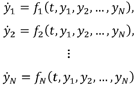
Our synthesis platform is formulated in terms of the general framework of N first-order complex ODEs $\begin{matrix} {\dot{y}}_{1} = f_{1} (t, y_{1}, y_{2}, \dots, y_{N}), \\ {\dot{y}}_{2} = f_{2} (t, y_{1}, y_{2}, \dots, y_{N}), \\ ⋮ \\ {\dot{y}}_{N} = f_{N} (t, y_{1}, y_{2}, \dots, y_{N}) \end{matrix}$
with state-space coordinates $y$ $_{1}, y_{2}, \dots, y_{N} \in ℂ .$
As before, the overdots here denote differentiation with respect to time t, ẏ = dy/dt. Given f_n(·) and an initial condition y_n(0) for all n = 1, 2,...,N, the above dynamical system can be numerically integrated returning N different complex outputs y₁(t), y₂(t),..., y_N(t). A sonic output s[k] = s(kT) can then be acquired at a sampling rate F_s = 1/T as a mixture of all oscillator outputs at each time index k as $s [k] = \sum_{n = 1}^{N} μ_{n} ℜ (y_{n} [k]),$
where y_n [k] = y_n (kT), µ_n is the user-defined gain of the n-th oscillator and
denotes the real part of a complex number. At first glance, the presented approach reveals a connection to additive synthesis; each equation in the system of ODEs may be associated to a different mode of vibration and a synthesis result can be obtained as a superposition of modes. On the other hand, in the context of non-linear dynamics, the same system is expected to be capable of producing quasi-periodic and even chaotic behavior. It will be shown what follows that the addition of simple non-linear terms may provide an efficient way for enriching the bandwidth of the sonic output and that non-linear coupling of ODEs is the cause of frequency modulation (FM) and amplitude modulation (AM).
By using the vector notation y = [y ₁,y ₂,...,y_N ] ^T and ẏ = [ẏ ₁,ẏ ₂,...,ẏ_N ] ^T the dynamic system above can be written in more compact form as $\dot{y} = F (y, t), y_{0} = f_{0} (r_{p}) .$
Before expanding F(·) into a more analytic form we first define the class of Nx1 vectors $y_{E}^{(m)} = {[{| y_{1} |}^{m_{1}}, {| y_{2} |}^{m_{2}}, \dots, {| y_{N} |}^{m_{N}}]}^{T}$
which are required for the mechanisms of pitchbend and non-linear decay. Here, the power m ₁,m ₂ ,...,m_N of each term can be varied explicitly by the user. An additional vector is required for handling amplitude control in the form $y_{c} = {[h (y_{1}, t, q, _{1}), h (y_{2}, t, q, _{2}), \dots, h (y_{N}, t, q_{N})]}^{T}$
where $h (y_{n}, t, a_{n}) = E (y_{n}) - a_{n} r_{p, n} + | E (y_{n}) - a_{n} r_{p, n} |$
will be used for penalizing the energy of the oscillation subject to the user-defined threshold a_n.
Based on the previous vector notations, the standard function F(y,t) can now be written as $\dot{y} = Ay + \frac{1}{t + ε} By + y ° C_{R} y_{E}^{(m)} + j y ° C_{I} y_{E}^{(l)} + y ° D (y + y *) + y ° E (y - y *) + y ° P y_{c} .$
Here (∘) denotes the Hadamard product. All bold capital letters are N×N coefficient matrices and m, l are N×1 coefficient vectors. These entities carry the synthesis control parameters.
The sound morphing potential of each term in Eq. (5.13) can already be guessed. In the general case, the coefficient matrices can be fully populated complex matrices. Observe that diagonal terms are responsible for processes that are intrinsic to each oscillator while non-diagonal terms in the matrices define the amount of coupling between ODEs. In the actual synthesis interface however, not all forms of coupling are used and synthesis parameters are restricted in most cases to the real domain. The parameter space is described in more detail in the next section together with a corresponding GUI.
The role of each term in the right hand side of the dynamical system is described below:

A is in general a complex NxN matrix. The diagonal terms of the matrix A_ii = σ_i + j2πf_i carry the decay rate and central frequency of each ODE while values inside non-diagonal terms define the additive coupling between ODEs.
B is a complex NxN diagonal matrix. The real part in each diagonal term is automatically calculated as a function of the user-defined attack time. This way, a different attack time can be used for each ODE.
C _R and C _I are both real NxN diagonal matrices. The values inside the diagonal of C _R are parameters associated to the non-linear decay effect while those of C _I are associated to tension modulation. To be noticed that the integer vectors m and n are also free user-defined parameters.
D is in general a fully populated real matrix of size NxN associated to the amplitude-modulation functionality. A non-zero value of D_ij indicates the degree with which the amplitude of the i-th ODE is modulated by the output of the j-th ODE.
E is a fully populated NxN real matrix which is associated to the frequency-modulation functionality. A non-zero value of E_ij indicates the degree with which the frequency of the i-th ODE is modulated by the output of the j-th ODE.

6. Graphical User Interface

A simple graphical user interface depicted in Figure 7 serves as prototype GUI for giving to the user access to all the control parameters of interest. The user is allowed to vary continuously the synthesis parameters from a minimum to a maximum value with the use of sliders. An exception is the synthesis parameters m_n and l_n which are associated to the rate of pitchbend and non-linear decay in Eq. (5.10). A pop-up window to set integer values is designed for that purpose.
The GUI is divided in two panels, the "Oscillator" panel and the "Coupling" panel. All sliders in the "Oscillator" panel refer to processes that are intrinsic to each oscillator. Namely, "attack time", "decay rate", "frequency", "pitch bend", "nonlinear decay" and "amplitude control" apply changes to the diagonal of matrices B, A, C _R , C _I and P respectively while the "intensity" slider is used for controlling the value of r_p,n . All the coefficient matrices are assumed to be confined in the real domain except from the diagonal of matrix A which obeys A_nn = σ_n + j2πf_n according to the user defined decay rate σ_n and frequency value f_n. The "amplitude threshold" and the "oscillator volume" sliders are associated to the values of a_n and µ_n in Eqs. (5.12) and (5.8), respectively. Finally, a set of radio buttons is used for selection of the oscillator index n. In the depicted example, the number of ODEs is limited to 4. A check box ("activate") controls whether a particular oscillator is active or not in the synthesis process.
On the right side, the "Coupling" panel includes the sliders that are necessary for controlling frequency modulation ("FM"). Amplitude modulation ("AM") and additive coupling ("AC"), therefore affecting the elements of matrices E, D and A respectively which are again confined between a minimum and maximum value in the real domain. An additional set of radio buttons is used for selecting the index of the "interfering oscillator. For example, if n is the index of the selected radio button in the "Oscillator" panel and j the corresponding index in the "Coupling" panel, the changes applied to the sliders will be reflected to the n-th row and j-th column of A, D and E. Observe that when n = j, changes applied to the "AC" slider are equivalent to changes in the decay rate of the n-th oscillator. A solution for this problem is either to deactivate the particular slider when n = j or to couple it with the "decay rate" slider. Observe that in the context of this synthesis approach there is no strict distinction between "modulating" and "carrier" oscillators. Any oscillator can be a "carrier" oscillator and a "modulating" oscillator at the same time. It might be of interest to use an ODE only as the means for modulating a different ODE. In that case, the output of the "modulating" ODE can be ignored by setting its gain to zero.
Some things are worth to be mentioned for the particular GUI example. It must have already been observed that while the number of synthesis parameters rises quadratically with the number of oscillators N, the actual number of graphical objects which is required is independent of that value. Also, in the current form, we have excluded coupling effects that are associated to matrices B, C _R, C _I and P, i.e. these matrices have by default zero values outside the main diagonal. Of potential interest here would be to include pitch bend and non-linear coupling in the oscillator panel which implies using fully populated matrices C _I and C _R respectively. In the case of non-linear decay, for example, the envelope of one oscillator would be allowed to affect the temporal characteristics of another oscillator.

7. Work-flow

The work-flow of the data collection approach is shown in Fig. 8(a). Any conventional digital recording equipment can be used in order to capture the natural sound of the percussive instrument. If done with a computer, a microphone will be required, and a sound card equipped with a microphone pre-amplifier. Alternatively, stand-alone devices can also be used. During the recording process, the musician is requested to perform several hits of varying impact level. This is advantageous in order to create a generic model which will output realistic synthesis results for a wide dynamic range.
Apart from recordings, already existing sample banks of percussive instrument can be exploited. There are numerous drum samplers in the market which are based on recordings of a variety of real percussive instruments. Based on these samplers, the necessary data can be exported by using any conventional Digital Audio Workstation (DAW) such as Cubase, Logic, GarageBand and others.
Some pre-processing of the recorded or exported audio file is also required. For this purpose, an automatic onset detection algorithm is built which can be used in order to crop a large audio file, containing multiple realizations of the physical instrument, into multiple smaller audio files, each one containing a single realization of the physical instrument. After these files have been created, they are named and saved in the hard disk for further processing.
The work-flow for the reconstruction process is shown in Fig. 8(b). The first step in the reconstruction process is to import the necessary audio samples from the instrument's database. In the second step, various temporal and frequency characteristics of the samples are plotted. Based on these plots, decisions such as the duration of the input signal, the number and the band-pass limits of the different frequency zones, the number and the type of the basis functions and many other parameters are taken.
The imported samples need to be processed according to the reconstruction parameters defined by the user, providing so the input data that will be used for the reconstruction process. In the context of a generic reconstruction approach, more than one audio samples of the same instrument might be required for the analysis, each time that a model is built. Special attention must be paid in that case so that all samples have the same duration and the same time onset.
Before the reconstruction process can begin, the type of reconstruction must be specified. This can be simple regression (least squares error minimization), constraint optimization or sparse reconstruction. More details about these three different approaches are shown further down.
The work-flow of the synthesis process is shown in Fig. 8(c). First, the model corresponding to a particular instrument is loaded. Before the synthesis process can begin, various parameters can be specified by the user. These concern the duration of the synthesized signal, the sampling rate and the impact level. Additional parameters which can be taken into account concern the decay rate and the pitch of the synthesized sound.
As long as the synthesis parameters are defined, the ODEs are integrated forward in time and the synthesis result is plotted and heard.

8. Appendix

Three different techniques for estimating the coefficients of an ODE are presented in the following. Other method can be used as well.

a) Regression: (Least squares) Error Minimization

The technique is illustrated for the general problem of N coupled ODEs, previously shown in Eq. 4.1. With respect to this problem, N different functions f_n(·) are defined and it is assumed that each function can be decomposed into M_n basis terms g_n(·). One considers all N time series y_n(t) (n = 1,2,...,N) measured at I time points t_i (i = 1,2,...,I). It is of course assumed that the derivative of y_n can be calculated at each time point. Then the process for the n-th ODE becomes minimization of the quantity $χ_{n}$ $_{2} = \sum_{i = 1}^{I} {\{\frac{{dy}_{n}}{dt} (t_{i}) - \sum_{m = 1}^{M_{n}} c_{nm} g_{nm} (y) (_{1}, y_{2}, \dots, y_{N}, \frac{{dy}_{1}}{dt}, \dots, \frac{{dy}_{N - 1}}{dt})\}}^{2} .$
A set of linear equations arises by the condition $\partial χ_{n}^{} / \partial c_{nm} = 0$
and the solution to these equations gives the optimal coefficients c_nm. While this is shown for the n-th ODE only, the process is identical for all N ODEs.
Neglecting dependence on the ODE index n, the problem is expressed in matrix vector form. The goal is to approximate the I×1 target observation vector ẏ as a linear combination of M basis vectors g _m, m = 1,2,...,M. Given the choice of basis vectors the goal is to find the values of the coefficients c_m, m = 1,2,...,M such that $\dot{y} \approx \sum_{m = 1}^{M} c_{m} g_{m},$
or in matrix form $\dot{y} = Wc$
where c = [c ₁ c ₂ ... c_m ] ^T ] and W = [ g ₁ g ₂ ... g _M ]. The number of time points I are considered to be greater than the number of basis vectors M and therefore, matrix W is overdetermined. The optimal coefficient vector c _o is derived through least squares error minimization as $c_{o} = {(W^{H} W)}^{- 1} W^{H} \dot{y}$
and the reconstruction error can be defined as $e = W c_{0} - \dot{y} .$
The least squares error criterion $E_{LS} = \frac{{‖ e ‖}_{2}}{{‖ \dot{y} ‖}_{2}} = \frac{\sqrt{\sum_{i = 1}^{I} e_{i}^{2}}}{\sqrt{\sum_{i = 1}^{I} y_{i}^{2}}}$
is used in order to measure the fit between the reconstructed signal and the target measurement. The square of the energy of the reconstruction error is normalized with respect to the energy of the target measurement; a value of E_LS equal to 0 therefore denotes a perfect reconstruction result.

b) Constrained optimization

There are certain occasions where one would desire to minimize the reconstruction error subject to linear constraints. This task can be mathematically formulated as $\min ({‖ \dot{y} - Wc ‖}_{2}) subject to Ac < B,$
where matrix A and vector B can be defined so as to express any linear inequalities. Constrained optimization can be used in order to restrict the sign of some coefficients in regions where the ODE remains stable. Additionally, one might use it in order to control the rate of decay or the fundamental frequency of the ODE, especially in low order ODEs where the coefficients of the basis functions have a well understood physical meaning. Apart from the use of inequalities, one can also fix the value of the ODE coefficients to a desired value.
This is a more general form of Eq. (8.6) which can be formulated as $\min ({‖ \dot{y} - Wc ‖}_{2}) subject to Ac < B and Cc = D .$
Constrained optimization can be performed by using the built-in Matlab routine lsqlin.

c) Optimization with a maximum allowed number of terms

There are occasions where one would like to approximate the target measurement y by using only a limited number of the M available candidate basis vectors g_m. This type of optimization is related to the so called sparse reconstruction techniques which have become extremely popular in the signal processing community. In general, sparse reconstruction techniques can be mathematically formulated as $\min ({‖ \dot{y} - Wc ‖}_{2}) + λ {‖ c ‖}_{o},$
where || c || _o measures the number of non-zero elements in vector c. While the applicability of this optimization strategy in signal compression and dimension reduction is apparent, it serves by helping to define ODEs with a small only number of terms, and therefore, with reduced computational complexity.
Among the many different algorithms that exist for sparse reconstruction, two popular greedy techniques are presented: Matching Pursuit (MP) and Orthogonal Matching Pursuit (OMP).
The MP algorithm (shown in Table 3) is an iterative technique based on three fundamental steps; an initialization step, a selection step and a residual update step. The algorithm requires that all basis vectors g _m are normalized to have equal energy. The algorithm begins by looking among all candidate basis vectors in order to find the one which has the highest correlation with the target measurement. A coefficient is returned by projecting the measurement onto the selected basis vector, and the contribution of the given vector to the measurement is removed, returning a residual. The same process is then repeated, but the initial measurement is now replaced by the residual calculated at the previous iteration. The process is repeated until a maximum number of iterations K_max has been reached.
OMP, shown in Table 4, has exactly the same initialization and selection step as MP, but the coefficients corresponding to the selected vectors are updated simultaneously by projecting the initial target measurement onto the space spanned by the entire set of selected vectors. The number of columns of the matrix with the collection of selected vectors D _Γi increases by one at each iteration. The value of the coefficients in OMP is thus allowed to vary at each iteration, whereas in MP, once a coefficient value has been defined, it is not allowed to change any more. OMP has in general better convergence properties than MP, but it includes a matrix inversion step which makes it slower than MP. Table 3

Matching Pursuit (MP)

Initialization

r ⁰ = ẏ , Γ ⁰ = 0̸

for i = 1 : K_max

Selection step

$k^{i} = {arg max}_{k} | g_{k}^{H} r^{i - 1} |$

Γ ⁱ =Γ^i-1∪kⁱ

Coefficient update

$c^{i} = g_{k^{i}}^{H} r^{i - 1}$

Residual update

r ⁱ = r ^i-1 - g _kicⁱ

end

Table 4

Orthogonal Matching Pursuit (OMP)

Initialization

r ⁰ = ẏ , Γ ⁰ = 0̸

for i = 1 : K_max

Selection step

$k^{i} = {arg max}_{k} | g_{k}^{H} r^{i - 1} |$

Γ ⁱ =Γ^i-1∪kⁱ

Coefficient update

$c^{i} = {(D_{^{r^{i}}}^{H} D_{^{r^{i}}})}^{- 1} D_{r^{i}}^{H} \dot{y}$

Residual update

rⁱ = ẏ - D _Γi c ⁱ

end

Claims

A method for synthetic modeling of a sound signal, wherein the method is performed by a processor of a computing device and comprises the following steps:
- providing an input sound sample as a target signal,

- analyzing the input sound sample to determine a model of a differential equation, wherein the differential equation is represented by at least one function, wherein the at least one function depends on at least one variable and at least one parameter,

- determining the at least one function, the at least one parameter and an initial condition of the differential equation so that the differential equation provides a dynamic model of the target signal, and

- determining the quality of the dynamic model using an optimality condition,
characterized in that
- at least one time-delayed version of the input sound sample is provided, and the at least one time-delayed version of the input sound sample is analyzed to determine the model of the differential equation and / or

- a time derivative of the input sound sample is determined, and the time derivative of the input sound sample is analyzed to determine the model of the differential equation, wherein the quality of the model of the differential equation is determined by an optimality condition.
The method of claim 1, wherein the model of the differential equation is a stochastic model and the at least one function is a non-linear function.
The method of claim 1 or 2, wherein the at least one parameter of the at least one function is changed dynamically according to a predefined function or to a user input.
The method of one of the preceding claims, further comprising decomposing the input sound sample into several components.
The method of one of the preceding claims, further comprising determining a number of dimensions of the model of the differential equation.
The method of one of the preceding claims, further comprising transforming a real valued component of the input sound sample into a complex value.
The method of one of the claims 1, 2 and 4 to 6, wherein the at least one parameter of the at least one function is a constant.
The method of one of the preceding claims, wherein the at least one function is a time-dependent function.
The method of one of the claims 1 to 7, wherein an envelope of the input sound sample is modeled by a dynamic equation, wherein the dynamic equation comprises at least one further differential equation.
The method of one of the preceding claims, further comprising outputting a sound signal which is generated by evolving the model of the differential equation in time.
System for synthetic modeling of a sound, comprising a processor and a memory and being configured to:
- provide an input sound sample as a target signal,

- analyze the input sound sample to determine a model of a differential equation, wherein the differential equation is represented by at least one function, wherein the at least one function depends on at least one variable and at least one parameter,

- determine the at least one function, the at least one parameter and an initial condition of the differential equation so that the differential equation provides a dynamic model of the target signal, and

- determine the quality of the dynamic model using an optimality condition characterized in that the system being further configured to

- provide at least one time-delayed version of the input sound sample, and analyze the at least one time-delayed version of the input sound sample to determine the model of the differential equation and / or

- determine a time derivative of the input sound sample, and analyze the time derivative of the input sound sample to determine the model of the differential equation, and, if applicable, determine the quality of the model of the differential equation by an optimality condition.
Computer program product which, when executed by a processor, executes the method according to one of the claims 1 to 10.