EP2960430A2 - Multilevel monotone constrained pressure residual multiscale techniques - Google Patents
Multilevel monotone constrained pressure residual multiscale techniques Download PDFInfo
- Publication number
- EP2960430A2 EP2960430A2 EP15174003.2A EP15174003A EP2960430A2 EP 2960430 A2 EP2960430 A2 EP 2960430A2 EP 15174003 A EP15174003 A EP 15174003A EP 2960430 A2 EP2960430 A2 EP 2960430A2
- Authority
- EP
- European Patent Office
- Prior art keywords
- pressure
- partial differential
- equations
- reservoir
- applying
- Prior art date
- Legal status (The legal status is an assumption and is not a legal conclusion. Google has not performed a legal analysis and makes no representation as to the accuracy of the status listed.)
- Granted
Links
Images



Classifications
-
- G—PHYSICS
- G06—COMPUTING OR CALCULATING; COUNTING
- G06F—ELECTRIC DIGITAL DATA PROCESSING
- G06F30/00—Computer-aided design [CAD]
- G06F30/20—Design optimisation, verification or simulation
-
- E—FIXED CONSTRUCTIONS
- E21—EARTH OR ROCK DRILLING; MINING
- E21B—EARTH OR ROCK DRILLING; OBTAINING OIL, GAS, WATER, SOLUBLE OR MELTABLE MATERIALS OR A SLURRY OF MINERALS FROM WELLS
- E21B47/00—Survey of boreholes or wells
- E21B47/06—Measuring temperature or pressure
-
- G—PHYSICS
- G06—COMPUTING OR CALCULATING; COUNTING
- G06F—ELECTRIC DIGITAL DATA PROCESSING
- G06F17/00—Digital computing or data processing equipment or methods, specially adapted for specific functions
- G06F17/10—Complex mathematical operations
Definitions
- Mathematical formulation of multicomponent multiphase flow in heterogeneous large-scale porous media can entail highly heterogeneous multiscale nonlinear and linear parameters. Development of efficient numerical solutions, hence, can depend on correct treatments of both highly heterogeneous multiscale parameters and strongly nonlinear coupling terms.
- the former challenge can be addressed in a variety of ways, e.g., the Multiscale Finite Element (MsFEM) and Finite Volume Methods (MsFVM) and the Multiscale Restriction Smoothed Basis (MsRSB).
- MsFEM Multiscale Finite Element
- MsFVM Finite Volume Methods
- MsRSB Multiscale Restriction Smoothed Basis
- multiscale methods for reservoir treat the coupling between flow and transport equations by adopting a sequential (IMPES- or Sequential-Implicit-type) strategy.
- IMPES- or Sequential-Implicit-type A high-stability sequential solution approach to reservoir simulation. Consequently, such approaches may be efficient when the coupling terms are not strong; however, when the coupling terms between flow and transport equations grow in importance, some sequential strategies may not be efficient. Strong coupling terms exist, e.g., in multiphase formulations with strong capillary and compositional effects. For these cases, fully implicit systems are generally more stable than sequential strategies.
- a computer-implemented method for modeling behavior of at least one fluid in a reservoir includes obtaining a plurality of measurements of a plurality of physical parameters at a plurality of locations within the reservoir, the plurality of physical parameters including at least pressure; discretizing a system of partial differential equations that model, based on the plurality of measurements, the plurality of physical parameters; iterating, for each of a plurality of time steps, and until convergence upon a solution to the system of partial differential equations: approximating a rough solution to the system of partial differential equations; applying a constrained pressure residual technique to extract a system of pressure linear equations from the rough solution to the system of partial differential equations; applying a pre-smoothing technique at a fine scale to determine an approximate solution to the system of pressure linear equations; applying multi-scale multi-level processing to improve the approximate solution to the system of pressure linear equations; applying a post-smoothing technique at a fine scale to further improve the approximate solution to the system
- the outputting may include displaying a representation of a behavior of the at least one fluid in the reservoir.
- the method may include predicting fluid behavior in the reservoir based on the system of partial differential equations; and extracting fluid from the reservoir based on the predicting.
- the iterating may be performed in parallel by at least one hardware graphics processing unit.
- the method may include history matching the system of partial differential equations.
- the physical parameters may include pressure, flow rate, and composition.
- the system of partial differential equations may include at least one of hyperbolic partial differential equation and parabolic partial differential equations.
- the reservoir may include heterogeneous anisotropic porous media.
- the iterating may include applying a flexible general minimal residual method.
- At least one of the applying a pre-smoothing technique and the applying a post-smoothing technique may include applying at least one technique selected from the group consisting of: applying ILU(0), applying a Jacobi smoother, and applying a Gauss-Seidel smoother.
- a computer system for modeling behavior of at least one fluid in a reservoir includes at least one electronic processor and persistent memory storing computer-interpretable instructions configured to cause the at least one processor to perform a method including: obtaining a plurality of measurements of a plurality of physical parameters at a plurality of locations within the reservoir, the plurality of physical parameters including at least pressure; discretizing a system of partial differential equations that model, based on the plurality of measurements, the plurality of physical parameters; iterating, for each of a plurality of time steps, and until convergence upon a solution to the system of partial differential equations: approximating a rough solution to the system of partial differential equations; applying a constrained pressure residual technique to extract a system of pressure linear equations from the rough solution to the system of partial differential equations; applying a pre-smoothing technique at a fine scale to determine an approximate solution to the system of pressure linear equations; applying multi-scale multi-level processing to improve the approximate solution to the system of pressure linear equations
- the outputting may include displaying a representation of a behavior of the at least one fluid in the reservoir.
- the instructions may be further configured to cause the at least one processor to perform: predicting fluid behavior in the reservoir based on the system of partial differential equations; and extracting fluid from the reservoir based on the predicting.
- the system may include at least one graphics processing unit, wherein the iterating is performed in parallel by the at least one hardware graphics processing unit.
- the instructions may be further configured to cause the at least one processor to perform history matching the system of partial differential equations.
- the physical parameters may include pressure, flow rate, and composition.
- the system of partial differential equations may include at least one of hyperbolic partial differential equation and parabolic partial differential equations.
- the reservoir may include heterogeneous anisotropic porous media.
- the iterating may include applying a flexible general minimal residual method.
- At least one of the applying a pre-smoothing technique and the applying a post-smoothing technique may include applying at least one technique selected from the group consisting of: applying ILU(0), applying a Jacobi smoother, and applying a Gauss-Seidel smoother.
- first, second, etc. may be used herein to describe various elements, these elements should not be limited by these terms. These terms are only used to distinguish one element from another.
- a first object or action could be termed a second object or action, and, similarly, a second object or action could be termed a first object or action, without departing from the scope of the invention.
- the first object or action, and the second object or action are both, objects or actions, respectively, but they are not to be considered the same object or action.
- the term “if” may be construed to mean “when” or “upon” or “in response to determining” or “in response to detecting,” depending on the context.
- the present disclosure provides computationally-efficient and highly-accurate techniques for modeling petroleum reservoir behavior.
- the present disclosure provides a consistent and robust numerical formulation for solutions to linear system of equations arising from the linearization of coupled nonlinear hyperbolic / parabolic (elliptic) partial differential equations (PDEs) of fluid flow in heterogeneous anisotropic porous media.
- the solutions may be used for both history matching and prediction.
- Some embodiments apply two-stage preconditioner and multiscale technology (e.g., multiscale restriction R and prolongation P operators).
- Parts I and II describe embodiments of the from different perspectives.
- Part III describes suitable technology for implementations.
- Numerical frameworks such as the following four examples can help analysis of nonlinear mixed hyperbolic / parabolic (elliptic) partial differential equations of fluid flow in heterogeneous anisotropic porous media:
- the ML-CPR-GMS and ML-CPR-NGMS may be viewed as extensions of the conventional linear solver technique (based on CPR technology combined with multigrid methods). Such techniques may utilize fundamental advantages of the multiscale technology. However, these methods are not unconditionally monotone methods.
- the MML-CPR-GMS and MML-CPR-NGMS can provide a good approximation of the pressure field and, hence, satisfy a discrete maximum principle and avoid spurious oscillations. This may be achieved by applying ML-CPR-GMS and ML-CPR-NGMS methods with the correction to the coarse level operator A c .
- the correction to the coarse level operator may be constructed in two actions.
- the first action may include choosing a sparsity pattern for the new coarse level operator A g , and the second action may remove or "collapse" entries, either in P T A P or R A P , that lie outside of that sparsity pattern in order to satisfy a discrete maximum principle.
- Unconventional reservoir simulations can involve several challenges not only arising from geological heterogeneities, but also from strong nonlinear physical coupling terms.
- the resulting governing reservoir equations may be of mixed hyperbolic / parabolic (elliptic) type thus making the initial-boundary value problem mathematically hard to solve.
- Existing upscaling and multiscale methods generally rely on a classical sequential formulation to treat the coupling between the nonlinear flow-transport equations.
- the sequential formulation is based on the decoupling of parabolic (or elliptic) variable such pressure from the hyperbolic variables such as saturations.
- the term f w f w ⁇ represents the fractional flow of water phase.
- the sequential formulation may be used to construct and solve the hyperbolic equations for the saturations (similar to Equation(4)) and elliptic (or parabolic) equation for the pressure (similar to Equation (5)). Unfortunately, the sequential strategies become inefficient when the flow and transport equations are strongly coupled. Examples of these cases include compositional displacements, and processes with strong capillarity effects.
- a user may choose from among the four aforementioned methods to obtain a solution for a particular physical situation.
- the CPR strategy may be used to formulate the pressure linear system of equations, the approximate conservative solution of which is obtained by employing a few iterations of the multi-level multiscale procedure.
- ILU(k), BILU(k), Gauss-Seidel, etc. smoothers combined with the global-stage (by way of non-limiting example, Multiscale Finite Volume, MsFV, and/or Multiscale Finite Element, MsFE, and/or Multiscale Restriction Smoothed Basis, MsRSB, etc.) multiscale procedure with different localization conditions (by way of non-limiting
- CPR-MS Constrained Pressure Residual Multiscale
- sequential formulation is less stable compared to a fully implicit CPR reduced system for strongly coupled nonlinear mixed hyperbolic / parabolic (elliptic) systems.
- the following approach may be used in reservoir simulations according to some embodiments.
- the number of Newton-Raphson iterations can be reduced further by solving the flash equations (Gibbs relations) before solving the fully coupled system.
- the following may be iteratively solved: ⁇ R f ⁇ X f ⁇
- X r i , X f i ⁇ ⁇ X f - R f ⁇
- X r i , X f i until X f is found such that R f X r i ⁇ X ⁇ f 0.
- Equation (9) This reduces Equation (9) to, by way of non-limiting example: ⁇ R r ⁇ X r ⁇ R r ⁇ X f ⁇ R f ⁇ X r ⁇ R f ⁇ X f ⁇
- X r i , X ⁇ f ⁇ ⁇ X r ⁇ ⁇ X f - R r 0 ⁇
- the variables ⁇ X f may be eliminated by Schur complement action (it is cheap and localized): ⁇ R r ⁇ X r - ⁇ R r ⁇ X f ⁇ ⁇ R f ⁇ X f - 1 ⁇ ⁇ R f ⁇ X r 0 ⁇ R f ⁇ X r ⁇ R f ⁇ X f ⁇
- Additional reduction actions e.g., constrained pressure residuals
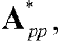
- a p ⁇ p * is defined as, by way of non-limiting example:
- a pp * A pp - QA sp
- a ps * A ps - QA ss
- R p * R p - Q ⁇ R s
- a p ⁇ p * C T ⁇ MAC .
- Several methods may be used to produce A p ⁇ p * , by way of non-limiting example:
- off-diagonal A ps terms can be ignored and the diagonal A ps part eliminated using the inverse of the block-diagonal of A.
- the resulting pressure matrix A p ⁇ p * may be solved with multiscale method as follows.
- the prolongation operator [P] may be constructed using different multiscale basis function, which can be obtained using (by way of non-limiting example) either Finite Volume or Finite Element Methods with different boundary conditions on the dual mesh or Restriction Smoothed Basis, or Meshless Basis Functions.
- the coarse pressure system Equation (24) can be solved exactly using different solver techniques (by way of non-limiting example, super ILU, AMG, etc.) or approximately using one V cycle of the AMG.
- Equations (15-16) After solving the pressure equation Equations (15-16), the remaining variables (i.e., saturations and molar fractions) can be recovered from Equations (5-11). It may not be required in the case of FULLIMP, IMPSAT to construct the total velocity field to compute hyperbolic variables.
- Fig. 1 illustrates an example partial set of actions for performing constrained proposed pressure residual Galerkin multiscale (CPR-GMS) and constrained pressure residual non-Galerkin multiscale (CPR-NGMS) methods.
- actions 1-2 and 8-12 can be the same as these shown in the original CPR-type.
- Actions 3 and 4 can utilize advantages of the multiscale technology as described herein.
- monotone method e.g., MML-CPR-NGMS and MML-CPR-GMS
- an algorithm can be applied to obtain final coarse level pressure.
- Basis functions needed for the construction of MS restriction [ R ] and prolongation [ P ] operators, can be computed at the beginning of each time step or at the beginning of the simulation and kept constant throughout the Newton-Raphson loop or simulation respectively.
- the update of basis functions can be done adaptively in some parts of the reservoir. Updating them at the end of each Newton-Raphson iteration may be useful when large time step sizes are used.
- the coarse system can be solved (action 5) with any of a number of various different strategies.
- the choice of the solver for the coarse pressure system may be related to the size of the coarse pressure matrix. This may depend both on the size of the model and on the choice of the coarsening factors. If the size of the coarse system is small enough, a direct solver can be used. For large cases, in order to obtain a small coarse pressure matrix, very large coarsening factors may be used. This may slow down the computation of basis functions as a direct solver is usually used for this action. In order to avoid this slow down, an iterative method may be used for the basis functions computation; in certain embodiments, this occurs at the beginning of the simulation process. Increasing the coarsening factors too much may affect the accuracy of the pressure solution and the number of nonlinear iterations.
- the fine scale pressure solution may be smoothed using, by way of non-limiting example, either Gauss-Seidel (GS) or ILU(0).
- GS Gauss-Seidel
- ILU(0) ILU(0)
- the pressure equations may be solved assuming only S W and S G are fixed.
- a coupled system for pressure may be formed (e.g., using p G and R s for GasWater cell state); see Equation (2).
- the variables R s may be eliminated by using a Schur complement (it is inexpensive and localized); see Equation (5).
- the resulting pressure Equations (15-16) matrix may be solved with a multiscale method, and then R s may be updated together with b G and b O . By doing this operation, the pressure equation (mechanical equilibrium) may feel the changes in the chemical equilibrium and vice versa.
- This operation is called second stage reduction in the prior art INTERSECT® simulator and it is generally not that expensive.
- the velocity may be computed using updated variable R s , p G , b O , and b G .
- the rest of computations may be the same as in the conventional prior art INTERSECT® multiscale implementation.
- This section describes a Multiscale (MS) method for fully implicit simulations of multiphase flow in highly heterogeneous porous media.
- MS Multiscale
- CPR Constrained Pressure Residual
- This pressure system is then coupled with a second stage solver for the full residual correction, as it is done in the classical CPR-based fully implicit solvers.
- some embodiments employ MsFEM or MsFVM or MsRBS to obtain an approximate solution of the CPR-based pressure system.
- the global solver may be based on a multiscale coarse-scale system (MsFVM or MsFEM or MsRBS), before and after which pre- and post-smoothing may be applied on the fine scale solution in order to eliminate high-frequency errors.
- MsFVM multiscale coarse-scale system
- MsFEM MsFEM
- MsRBS multiscale coarse-scale system
- J pp is the pressure block coefficients
- J ss is the non-pressure block (saturations or components molar fractions) coefficients
- J ps and J sp represent the respective coupling coefficients.
- the terms ⁇ x p and ⁇ x s represent the increments of pressure (primary variables or physical parameters) and of the other (secondary) variables or physical parameters (e.g., saturations and components molar fractions).
- the linear solver action represents a dominant part of the whole computational time. Performance of iterative linear solvers strongly depends on robust and fast preconditioners, amenable for massive parallelization. Additionally, for realistic-scale problems, the memory requirement to store the sparse Jacobian linear systems becomes an important consideration.
- Linear solvers generally used in reservoir simulations consist of preconditioned Krylov subspace methods such as ORTHOMIN with nested factorization as a preconditioner.
- a significant improvement in preconditioning strategy of linear systems arising from reservoir simulations was made by introducing the Constrained Pressure Residual preconditioning (CPR) method.
- the CPR preconditioner acknowledges the fact that Equation (32) is of a mixed parabolic (or elliptic)-hyperbolic type.
- the CPR method improves the convergence rate for the full linear system, based on a pressure predictor-corrector strategy for each linear step.
- Q J ps ⁇ J ss - 1 ⁇ Q ⁇ I
- with colsum J ps ⁇ colsum ⁇ J ss - 1 ,
- J p ⁇ s * is approximately equal to zero, i.e., J pp * ⁇ ⁇ ⁇ x p ⁇ r p *
- some embodiments ignore the off-diagonal J ps terms and eliminate the diagonal part of J ps using the inverse of the block-diagonal of J ss .
- Equation (36) is the pressure equation. It forms an approximation of the parabolic (or elliptic for incompressible flow) part of the discrete operator and may be considered separately from the remaining hyperbolic part.
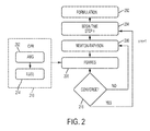
- Fig. 2 is a schematic diagram illustrating a method for flexible generalized minimal residual (FGMRES) preconditioned by a two-stage constrained pressure residual preconditioner.
- the linear system of Equation (32) (formulation 202) may be solved by flexible generalized minimal residual 208 (FGMRES), preconditioned by the CPR method 210.
- the preconditioner can include two complementary stages. The first stage 212 may be used to approximate the pressure solution by commonly applying Algebraic Multigrid (AMG) method to Equation (36). In the second stage 214, another preconditioner (e.g., the ILU(O) method) may be applied to the full system of Equation (32) such that the first stage pressure approximation is used as the initial guess.
- AMG Algebraic Multigrid
- another preconditioner e.g., the ILU(O) method
- Fig. 2 illustrates the process for a given time step 204, in which is nested a Newton-Raphson loop 206 with attendant convergence detection 2
- a linear solver based on CPR-AMG preconditioning may be effective in terms of algorithmic efficiency.
- the second stage of CPR preconditioning often incudes a variant of an incomplete LU factorization, which again is non-trivial to parallelize.
- the linear solver is still some way from near-ideal scalability.
- CPR-MS Constrained Pressure Residual Multiscale
- multiscale methods use an approximation space that is spanned by basis functions.
- Some embodiments use multiscale finite element basis functions to create an approximation space for pressure of much lower dimension than the original simulation grid.
- the approximation space may be constructed using a discretization for pressure to capture the effect of fine-scale heterogeneity locally.
- the discretization for pressure basis functions may be obtained from sequential formulation.
- the pressure residual is formed like in IMPES formulation by eliminating the unknown saturation from the mass balance equations.
- the pressure matrix may be the Jacobian of the pressure residual.
- Fig. 3 schematically illustrates a simulation grid with both a fine partition and coarse overlapping subdomains.
- the simulation grid is partitioned into overlapping subdomains 302, where the cells (e.g., 306) in the overlap region 308 form a coarse mesh.
- the MsFV method uses a non-overlapping partition 304.
- each grid cell is classified as an inner cell if it is not part of the overlap between subdomains.
- the overlapping region between subdomains is partitioned into a set of face subdomains that form an overlap only between two partitions, the remaining cells (wirebasket) are partitioned into edge subdomains connected by corner cells (Jenny et al., 2003).
- each basis function ⁇ i k is a discrete solution to a homogeneous pressure equation in the interior of D k and solves a reduced pressure equation on the face and edge subdomains on the boundary of D k (Hou and Wu, 1997).
- the discrete subdomain basis functions created in this way are continuous across subdomain boundaries and we have by construction for each subdomain D k ⁇ D .
- the coarse scale approximation space includes constant functions.
- Some embodiments utilize restriction operators R to form a linear system for the pressure in the wirebasket corner cells.
- Two different restriction operators may be used, by way of non-limiting example.
- R FE P T .
- the application of R FE to a vector x yields a weighted sum ofx for cells near each wirebasket corner cell. Applied to a linear system, it yields a classical Galerkin type coarse scale approximation.
- the other useful restriction operator is a finite-volume type restriction R FV .
- R FV finite-volume type restriction
- Fig. 4 is a schematic diagram illustrating constrained proposed pressure residual Galerkin multiscale (CPR-GMS) and constrained pressure residual non-Galerkin multiscale (CPR-NGMS) methods.
- Blocks 402, 404, 406, 408, and 418 are essentially the same as blocks 202, 204, 206, 208 and 218 of Fig. 2 .
- the CPR-MS algorithm combines both actions of the CPR-AMG method and of multiscale methods.
- a fully implicit system may be solved with a CPR type 2-stage preconditioners where a MS method is used for solving the pressure system extracted by the CPR decoupling operator.
- the whole solution strategy can be summarized as follows (the below actions are referred to herein as the "Example Process Summary").
- Actions 1, 5 and 6 of the Example Process Summary may be performed as in the original CPR-type solver implemented in INTERSECT. Actions 2 and 3 may be performed as in typical multiscale methods (block 414 of Fig. 4 ). Thus, the original two-stage preconditioning structure of the solution strategy may be altered to utilize a different choice for the solution of the pressure system.
- Basis functions, used for the construction of MS restriction (R) and prolongation (P) operators, may be computed at the beginning of each time step and kept constant throughout the Newton-Raphson loop. Updating them at the end of each Newton-Raphson iteration may be useful when large time step sizes are used.
- the coarse system can be solved (action 3 of the above Example Process Summary) with different strategies.
- the choice of the solver for the coarse pressure system is strictly related to the size of the coarse pressure matrix; this depends both on the size of the model and on the choice of the coarsening factors. If the size of the coarse system is small enough a direct solver can be used; for big cases, in order to obtain a small coarse pressure matrix, very large coarsening factors may be used. This may slow down the computation of basis functions because a direct solver is usually used for this action; in order to avoid this slow down, an iterative method may be used for the basis functions computation. The advantage of doing that is that basis functions calculation is only done once per each time step, whereas a different coarse system may be solved for each Newton iteration. However, increasing too much the coarsening factors may affect the accuracy of our pressure solution and the number of nonlinear iterations may grow.
- pre- and post-smoothing actions (blocks 412 and 416, respectively) on the fine scale pressure solution are depicted in the above summary.
- the fine scale pressure solution is smoothed using either Gauss Seidel (GS) or ILU(0) before and after action 3 of the above Example Process Summary.
- GS Gauss Seidel
- ILU(0) ILU(0)
- Fig. 5 illustrates an example reservoir representation depicting a fine grid of 648,000 cells. That is, Fig. 5 depicts a fine grid utilized for the test case.
- the grid 502 was 144 ⁇ 150 ⁇ 30, for a total of 648,000 cells.
- Results and performance were compared with the current version of the INTERSECT® (IX) simulator, which uses CPR preconditioning with a IV-cycle AMG for solving the pressure system and ILU(0) as a second stage preconditioner.
- IX INTERSECT®
- the same second stage preconditioner was used so that the only difference is solution strategy of the pressure system.
- Two different values for the minimum time step size were used which resulted in two completely different time step selections throughout the simulation. The maximum time step size was always kept the same.
- Fig. 6 illustrates graphs depicting field pressure and gas block saturation solutions for CPR-AMG and CPR-MS.
- Graph 602 depicts average pressure of the entire reservoir.
- Graph 604 depicts a gas saturation profile of a particular location, (120.65, 1). As depicted in Fig. 6 , the two solutions completely match; no exceptions to complete overlap of the curves are visible in Fig. 6 , in either graph 602 or 604.
- Table 2 depicts the results in terms of performance (number of iterations and CPU time) for the four performed runs and for the current INTERSECT configuration (CPR-AMG). Table 2 Results of all runs for a minimum time step size of 15 days Number of iterations CPU time (s) Runs Non linear iter. Linear iter . Linear Solver total Run 1 369 2872 1615 2699 Run 2 369 2845 1119 2203 Run 3 371 3327 1233 2309 Run 4 371 3649 2026 3114 IX 369 2187 1571 2537
- the CPR-MS algorithm uses a greater number of linear iterations than the original Intersect CPR-AMG; this was actually expected as MS methods usually require a great number of linear iterations. Pre and post-smoothing help limiting the growth in the number of linear iterations.
- Fig. 7 is a flowchart depicting a method according to some embodiments.
- the method may be implemented using hardware specialized for parallel processing, such as that described below in reference to Fig. 8 .
- the method may be applied obtain solutions to a linear system of equations arising from the linearization of coupled nonlinear hyperbolic / parabolic (elliptic) partial differential equations (PDEs) of fluid flow in heterogeneous anisotropic porous media. More generally, the method may be applied model the behavior of a petroleum reservoir.
- PDEs coupled nonlinear hyperbolic / parabolic (elliptic) partial differential equations
- the method obtains measurements of physical parameters of the reservoir at various locations within the reservoir and at various times.
- the number of measurements can range from hundreds to billions.
- the measured physical parameters can include pressure, phase saturations and phase-specific molar fractions, e.g., as described above in Section I.
- Various techniques may be utilized to obtain such measurements, such as the use of down-hole sensors.
- the method discretizes a system of partial differential equations that are formed according to the measurements obtained at block 702. More particularly, the method may form a system of partial differential equations as described above in reference to Equations (1-3) generally, or, more particularly, Equations (4-7).
- the discretization technique applied to such a system of equations may include, by way of non-limiting example, a finite-volume, second-order state, first-order time technique. More generally, the system of partial differential equations may be discretized using techniques described above in reference to Equation (8).
- the method establishes one or more nested loops for processing at each of a plurality of time steps and each of a plurality of physical parameter values.
- Such nested loops are depicted graphically in, and described in reference to, Figs. 2 and 4 , for example.
- the outer loop may iterate per time step, while the inner loop may perform iterations of the Newton-Raphson technique.
- Each Newton-Raphson iteration may compute a solution to Equation (9) using Equations (10-14), for example.
- GPUs Graphical Processing Units
- the method approximates a rough solution (initial guess), e.g., to Equation (9) for the time step currently being processed.
- the technique may utilize a preconditioning process as described herein.
- the solution from the previous time step may be assumed as initial guess.
- the method updates the residuals.
- the actions of this block may be performed as is implicit in action 3 of Fig. 1 . (Note that the actions of this block are distinct from action 8 of Fig. 1 .)
- the method extracts a system of linear equations representing pressure.
- the actions of this block may be performed as described herein in reference to Equations (15-20), action 2 of Fig. 2 , block 410 of Fig. 4 , and action 1 of the Example Process Summary. More generally, the actions of this block correspond to at least part of the Constrained Pressure Residual (CPR) technique described herein.
- CPR Constrained Pressure Residual
- the method applies a pre-smoothing technique.
- the actions of this block may be performed as described herein in reference to action 3 of Fig. 1 , and block 412 of Fig. 4 .
- the method applies multi-scale multi-level processing.
- the actions of this block may be performed as described herein in reference to Equations (21-28), action 3 of the Example Process Summary, actions 4-6 of Fig. 1 , and block 414 of Fig. 4 .
- the method applies a post-smoothing technique.
- the actions of this block may be performed as described herein in reference to action 7 of Fig. 1 , and block 416 of Fig. 4 .
- the method solves for the remaining physical parameters.
- the actions of this block may be performed as described herein in reference to action 6 of the Example Process Summary, and actions 10 and 11 of Fig. 1 .
- the technique determines whether to repeat the iteration(s) initiated at block 706. This may include determining whether the Newton-Raphson technique has sufficiently converged. The actions of this block may be performed as described herein in reference to action 12 of Fig. 1 , and block 418 of Fig. 4 .
- the method outputs the solution.
- the outputting may take on various forms.
- the outputting may include displaying a pictorial representation of all or part of the reservoir, displaying one or more graphs depicting one or more physical parameters, delivering data to a separate process (e.g., to determine whether to extract petroleum), or other outputting techniques.
- Fig. 8 illustrates a schematic view of a computing or processor system 800, according to an embodiment.
- the processor system 800 may include one or more processors 802 of varying core configurations (including multiple cores) and clock frequencies.
- the one or more processors 802 may be operable to execute instructions, apply logic, etc. It will be appreciated that these functions may be provided by multiple processors or multiple cores on a single chip operating in parallel and/or communicably linked together.
- the one or more processors 802 may be or include one or more GPUs.
- the processor system 800 may also include a memory system, which may be or include one or more memory devices and/or computer-readable media 804 of varying physical dimensions, accessibility, storage capacities, etc. such as flash drives, hard drives, disks, random access memory, etc., for storing data, such as images, files, and program instructions for execution by the processor 802.
- the computer-readable media 804 may store instructions that, when executed by the processor 802, are configured to cause the processor system 800 to perform operations. For example, execution of such instructions may cause the processor system 800 to implement one or more portions and/or embodiments of the methods described herein.
- the processor system 800 may also include one or more network interfaces 806.
- the network interfaces 806 may include any hardware, applications, and/or other software. Accordingly, the network interfaces 806 may include Ethernet adapters, wireless transceivers, PCI interfaces, and/or serial network components, for communicating over wired or wireless media using protocols, such as Ethernet, wireless Ethernet, etc.
- the processor system 800 may further include one or more peripheral interfaces 808, for communication with a display screen, projector, keyboards, mice, touchpads, sensors, other types of input and/or output peripherals, and/or the like.
- peripheral interfaces 808 for communication with a display screen, projector, keyboards, mice, touchpads, sensors, other types of input and/or output peripherals, and/or the like.
- the components of processor system 800 need not be enclosed within a single enclosure or even located in close proximity to one another, but in other implementations, the components and/or others may be provided in a single enclosure.
- the memory device 804 may be physically or logically arranged or configured to store data on one or more storage devices 810.
- the storage device 810 may include one or more file systems or databases in any suitable format.
- the storage device 810 may also include one or more software programs 812, which may contain interpretable or executable instructions for performing one or more of the disclosed processes. When requested by the processor 802, one or more of the software programs 812, or a portion thereof, may be loaded from the storage devices 810 to the memory devices 804 for execution by the processor 802.
- processor system 800 may also be implemented in part or in whole by electronic circuit components or processors, such as application-specific integrated circuits (ASICs) or field-programmable gate arrays (FPGAs).
- ASICs application-specific integrated circuits
- FPGAs field-programmable gate arrays
Landscapes
- Engineering & Computer Science (AREA)
- Physics & Mathematics (AREA)
- Theoretical Computer Science (AREA)
- Mining & Mineral Resources (AREA)
- Geology (AREA)
- Life Sciences & Earth Sciences (AREA)
- General Physics & Mathematics (AREA)
- Data Mining & Analysis (AREA)
- Mathematical Physics (AREA)
- General Engineering & Computer Science (AREA)
- Geophysics (AREA)
- Geochemistry & Mineralogy (AREA)
- General Life Sciences & Earth Sciences (AREA)
- Fluid Mechanics (AREA)
- Environmental & Geological Engineering (AREA)
- Mathematical Optimization (AREA)
- Software Systems (AREA)
- Databases & Information Systems (AREA)
- Pure & Applied Mathematics (AREA)
- Mathematical Analysis (AREA)
- Computational Mathematics (AREA)
- Algebra (AREA)
- Geometry (AREA)
- Evolutionary Computation (AREA)
- Computer Hardware Design (AREA)
- Management, Administration, Business Operations System, And Electronic Commerce (AREA)
- Medicinal Preparation (AREA)
Abstract
Description
- The present application claims priority to and the benefit of
U.S. Provisional Patent Application No. 62/018,318 - Mathematical formulation of multicomponent multiphase flow in heterogeneous large-scale porous media can entail highly heterogeneous multiscale nonlinear and linear parameters. Development of efficient numerical solutions, hence, can depend on correct treatments of both highly heterogeneous multiscale parameters and strongly nonlinear coupling terms. The former challenge can be addressed in a variety of ways, e.g., the Multiscale Finite Element (MsFEM) and Finite Volume Methods (MsFVM) and the Multiscale Restriction Smoothed Basis (MsRSB).
- In general, multiscale methods for reservoir treat the coupling between flow and transport equations by adopting a sequential (IMPES- or Sequential-Implicit-type) strategy. A high-stability sequential solution approach to reservoir simulation. Consequently, such approaches may be efficient when the coupling terms are not strong; however, when the coupling terms between flow and transport equations grow in importance, some sequential strategies may not be efficient. Strong coupling terms exist, e.g., in multiphase formulations with strong capillary and compositional effects. For these cases, fully implicit systems are generally more stable than sequential strategies.
- In accordance with some embodiments, a computer-implemented method for modeling behavior of at least one fluid in a reservoir is disclosed. The method includes obtaining a plurality of measurements of a plurality of physical parameters at a plurality of locations within the reservoir, the plurality of physical parameters including at least pressure; discretizing a system of partial differential equations that model, based on the plurality of measurements, the plurality of physical parameters; iterating, for each of a plurality of time steps, and until convergence upon a solution to the system of partial differential equations: approximating a rough solution to the system of partial differential equations; applying a constrained pressure residual technique to extract a system of pressure linear equations from the rough solution to the system of partial differential equations; applying a pre-smoothing technique at a fine scale to determine an approximate solution to the system of pressure linear equations; applying multi-scale multi-level processing to improve the approximate solution to the system of pressure linear equations; applying a post-smoothing technique at a fine scale to further improve the approximate solution to the system of pressure linear equations; and solving the system of partial differential equations for remaining physical parameters based on the further improved approximate solution to the system of pressure linear equations; and outputting the solution to the system of partial differential equations.
- Various optional features of the above embodiments include the following. The outputting may include displaying a representation of a behavior of the at least one fluid in the reservoir. The method may include predicting fluid behavior in the reservoir based on the system of partial differential equations; and extracting fluid from the reservoir based on the predicting. The iterating may be performed in parallel by at least one hardware graphics processing unit. The method may include history matching the system of partial differential equations. The physical parameters may include pressure, flow rate, and composition. The system of partial differential equations may include at least one of hyperbolic partial differential equation and parabolic partial differential equations. The reservoir may include heterogeneous anisotropic porous media. The iterating may include applying a flexible general minimal residual method. At least one of the applying a pre-smoothing technique and the applying a post-smoothing technique may include applying at least one technique selected from the group consisting of: applying ILU(0), applying a Jacobi smoother, and applying a Gauss-Seidel smoother.
- According to some embodiments, a computer system for modeling behavior of at least one fluid in a reservoir is disclosed. The system includes at least one electronic processor and persistent memory storing computer-interpretable instructions configured to cause the at least one processor to perform a method including: obtaining a plurality of measurements of a plurality of physical parameters at a plurality of locations within the reservoir, the plurality of physical parameters including at least pressure; discretizing a system of partial differential equations that model, based on the plurality of measurements, the plurality of physical parameters; iterating, for each of a plurality of time steps, and until convergence upon a solution to the system of partial differential equations: approximating a rough solution to the system of partial differential equations; applying a constrained pressure residual technique to extract a system of pressure linear equations from the rough solution to the system of partial differential equations; applying a pre-smoothing technique at a fine scale to determine an approximate solution to the system of pressure linear equations; applying multi-scale multi-level processing to improve the approximate solution to the system of pressure linear equations; applying a post-smoothing technique at a fine scale to further improve the approximate solution to the system of pressure linear equations; and solving the system of partial differential equations for remaining physical parameters based on the further improved approximate solution to the system of pressure linear equations; and outputting the solution to the system of partial differential equations.
- Various optional features of the above embodiments include the following. The outputting may include displaying a representation of a behavior of the at least one fluid in the reservoir. The instructions may be further configured to cause the at least one processor to perform: predicting fluid behavior in the reservoir based on the system of partial differential equations; and extracting fluid from the reservoir based on the predicting. The system may include at least one graphics processing unit, wherein the iterating is performed in parallel by the at least one hardware graphics processing unit. The instructions may be further configured to cause the at least one processor to perform history matching the system of partial differential equations. The physical parameters may include pressure, flow rate, and composition. The system of partial differential equations may include at least one of hyperbolic partial differential equation and parabolic partial differential equations. The reservoir may include heterogeneous anisotropic porous media. The iterating may include applying a flexible general minimal residual method. At least one of the applying a pre-smoothing technique and the applying a post-smoothing technique may include applying at least one technique selected from the group consisting of: applying ILU(0), applying a Jacobi smoother, and applying a Gauss-Seidel smoother.
- This summary is provided to introduce a selection of concepts that are further described below in the detailed description. This summary is not intended to identify key or essential features of the claimed subject matter, nor is it intended to be used as an aid in limiting the scope of the claimed subject matter.
- The accompanying drawings, which are incorporated in and constitute a part of this specification, illustrate embodiments of the present teachings and together with the description, serve to explain the principles of the present teachings.
-
Fig. 1 illustrates an example partial set of actions for performing constrained proposed pressure residual Galerkin multiscale (CPR-GMS) and constrained pressure residual non-Galerkin multiscale (CPR-NGMS) methods. -
Fig. 2 is a schematic diagram illustrating a method for flexible generalized minimal residual (FGMRES) preconditioned by a two-stage constrained pressure residual preconditioner. -
Fig. 3 schematically illustrates a simulation grid with both a fine partition and coarse overlapping and non-overlapping subdomains. -
Fig. 4 is a schematic diagram illustrating constrained proposed pressure residual Galerkin multiscale (CPR-GMS) and constrained pressure residual non-Galerkin multiscale (CPR-NGMS) methods. -
Fig. 5 illustrates an example reservoir representation depicting a fine grid of 648,000 cells. -
Fig. 6 illustrates graphs depicting field pressure and gas block saturation solutions for CPR-AMG and CPR-GMS. -
Fig. 7 is a flowchart depicting a method according to some embodiments. -
Fig. 8 illustrates a schematic view of a computing orprocessor system 100, according to an embodiment. - Reference will now be made in detail to embodiments, examples of which are illustrated in the accompanying drawings and figures. In the following detailed description, numerous specific details are set forth in order to provide a thorough understanding of the invention. However, it will be apparent to one of ordinary skill in the art that the invention may be practiced without these specific details. In other instances, well-known methods, procedures, components, circuits and networks have not been described in detail so as not to unnecessarily obscure aspects of the embodiments.
- It will also be understood that, although the terms first, second, etc. may be used herein to describe various elements, these elements should not be limited by these terms. These terms are only used to distinguish one element from another. For example, a first object or action could be termed a second object or action, and, similarly, a second object or action could be termed a first object or action, without departing from the scope of the invention. The first object or action, and the second object or action, are both, objects or actions, respectively, but they are not to be considered the same object or action.
- The terminology used in the description of the invention herein is for the purpose of describing particular embodiments only and is not intended to be limiting of the invention. As used in the description of the invention and the appended claims, the singular forms "a," "an" and "the" are intended to include the plural forms as well, unless the context clearly indicates otherwise. It will also be understood that the term "and/or" as used herein refers to and encompasses any and all possible combinations of one or more of the associated listed items. It will be further understood that the terms "includes," "including," "comprises" and/or "comprising," when used in this specification, specify the presence of stated features, integers, actions, operations, elements, and/or components, but do not preclude the presence or addition of one or more other features, integers, actions, operations, elements, components, and/or groups thereof.
- As used herein, the term "if" may be construed to mean "when" or "upon" or "in response to determining" or "in response to detecting," depending on the context.
- Attention is now directed to processing procedures, methods, techniques and workflows that are in accordance with some embodiments. Some operations in the processing procedures, methods, techniques and workflows disclosed herein may be combined and/or the order of some operations may be changed.
- The present disclosure provides computationally-efficient and highly-accurate techniques for modeling petroleum reservoir behavior. In particular, the present disclosure provides a consistent and robust numerical formulation for solutions to linear system of equations arising from the linearization of coupled nonlinear hyperbolic / parabolic (elliptic) partial differential equations (PDEs) of fluid flow in heterogeneous anisotropic porous media. The solutions may be used for both history matching and prediction. Some embodiments apply two-stage preconditioner and multiscale technology (e.g., multiscale restriction R and prolongation P operators).
- This disclosure is set forth in three parts. Parts I and II describe embodiments of the from different perspectives. Part III describes suitable technology for implementations.
- Numerical frameworks such as the following four examples can help analysis of nonlinear mixed hyperbolic / parabolic (elliptic) partial differential equations of fluid flow in heterogeneous anisotropic porous media:
- (1) Multilevel Constrained Pressure Residual Galerkin Multiscale (ML-CPR-GMS) when R = P T ,
- (2) Multilevel Constrained Pressure Residual Non-Galerkin Multiscale (ML-CPR-NGMS) when R ≠ P T ,
- (3) Monotone Multilevel Constrained Pressure Residual Galerkin Multiscale (MML-CPR-GMS) when Ag ≠ Ac = P T A P (where Ac and Ag are the original and monotone coarse level pressure operators respectively), and
- (4) Multilevel Constrained Pressure Residual Non-Galerkin Multiscale (MML-CPR-NGMS) when Ag ≠ Ac = R A P.
- The ML-CPR-GMS and ML-CPR-NGMS may be viewed as extensions of the conventional linear solver technique (based on CPR technology combined with multigrid methods). Such techniques may utilize fundamental advantages of the multiscale technology. However, these methods are not unconditionally monotone methods. The MML-CPR-GMS and MML-CPR-NGMS can provide a good approximation of the pressure field and, hence, satisfy a discrete maximum principle and avoid spurious oscillations. This may be achieved by applying ML-CPR-GMS and ML-CPR-NGMS methods with the correction to the coarse level operator Ac . The correction to the coarse level operator may be constructed in two actions. The first action may include choosing a sparsity pattern for the new coarse level operator Ag , and the second action may remove or "collapse" entries, either in P T A P or R A P, that lie outside of that sparsity pattern in order to satisfy a discrete maximum principle.
- Such an approach may be useful in reservoir simulation. Unconventional reservoir simulations can involve several challenges not only arising from geological heterogeneities, but also from strong nonlinear physical coupling terms. The resulting governing reservoir equations may be of mixed hyperbolic / parabolic (elliptic) type thus making the initial-boundary value problem mathematically hard to solve. Existing upscaling and multiscale methods generally rely on a classical sequential formulation to treat the coupling between the nonlinear flow-transport equations. The sequential formulation is based on the decoupling of parabolic (or elliptic) variable such pressure from the hyperbolic variables such as saturations. In a simple case of immiscible incompressible two-phase flow (oil-water) with no capillary pressure and gravity in a heterogeneous incompressible porous media, the PDEs may be written as follows, by way of non-limiting example:


In Equations (1-3), the terms Sβ , gβ (X ), λβ denote, respectively, the saturation, source/sink term, mobility of fluid phase β, where β = w,o for water and oil. The term φ represents the porosity. Due to Sw + So = 1, an equivalent statement to the system Equations (1-3) may be given as, by way of non-limiting example:

- In Equations (4) and (5), the term


represents the total mobility. The term
- To extend the applicability of the multiscale methods for these challenging cases, a number of methods for modeling strongly coupled nonlinear mixed hyperbolic / parabolic (elliptic) system are proposed in this disclosure:
- (a) Multilevel Constrained Pressure Residual Galerkin Multiscale (ML-CPR-GMS) when R = P T ;
- (b) Multilevel Constrained Pressure Residual Non-Galerkin Multiscale (ML-CPR-NGMS) when R ≠ P T ,
- (c) Monotone Multilevel Constrained Pressure Residual Galerkin Multiscale (MML-CPR-GMS) when Ag ≠ Ac = P T A P (where Ac and Ag are the original and monotone coarse level pressure operators respectively),
- (d) Monotone Multilevel Constrained Pressure Residual Non-Galerking Multiscale (MML-CPR-NGMS) when Ag ≠ Ac = R A P.
- According to some embodiments, a user may choose from among the four aforementioned methods to obtain a solution for a particular physical situation. In these methods, the CPR strategy may be used to formulate the pressure linear system of equations, the approximate conservative solution of which is obtained by employing a few iterations of the multi-level multiscale procedure. According to some embodiments, any of several local (by way of non-limiting example, ILU(k), BILU(k), Gauss-Seidel, etc.) smoothers combined with the global-stage (by way of non-limiting example, Multiscale Finite Volume, MsFV, and/or Multiscale Finite Element, MsFE, and/or Multiscale Restriction Smoothed Basis, MsRSB, etc.) multiscale procedure with different localization conditions (by way of non-limiting example, Linear BC, Reduced Problem BC, etc.) for basis functions may be employed in order to find an optimum strategy for the highly nonlinear compositional displacements.
- In general, sequential formulation is less stable compared to a fully implicit CPR reduced system for strongly coupled nonlinear mixed hyperbolic / parabolic (elliptic) systems. The following approach may be used in reservoir simulations according to some embodiments.
- (1) To avoid instabilities during the compositional multi-phase / multi-component flow (e.g., some flips in the cell phase state), both mechanical and chemical equilibrium may be used for convergence purpose. Hence, some embodiments perform smoothing action (e.g., at the fine scale).
- (2) The pressure equation may be formed using the CPR method. Assuming that for each time step an embodiment solves the following set of non-linear equations constructing using IMPES, IMPSAT or FULLIMP discretization methods, then

- The number of Newton-Raphson iterations can be reduced further by solving the flash equations (Gibbs relations) before solving the fully coupled system. In some embodiments, for each Newton-Raphson iteration i, the following may be iteratively solved:

untilX f is found such that
- This reduces Equation (9) to, by way of non-limiting example:

The variables ΔXf may be eliminated by Schur complement action (it is cheap and localized):
The resulting reservoir matrix may be further analysed before applying multiscale method:

- Reservoir variables (physical parameters) may be generally a combination of pressure, phase saturations and some of the phase specific molar fractions, i.e.,


where


to obtain
Now the pressure matrix may be extracted as follows, by way of non-limiting example:
where C T = [I 0]. - The effectiveness of the CPR methods can depend on the quality of the pressure matrix

- (a) Quasi-IMPES
- (b) True-IMPES.
- In certain embodiments, for Quasi-IMPES scheme, off-diagonal A ps terms can be ignored and the diagonal A ps part eliminated using the inverse of the block-diagonal of A.
- The resulting pressure matrix


where the basis functions


The system of Equation (22) may be re-written in the compact form as follows
where


- The prolongation operator [P] may be constructed using different multiscale basis function, which can be obtained using (by way of non-limiting example) either Finite Volume or Finite Element Methods with different boundary conditions on the dual mesh or Restriction Smoothed Basis, or Meshless Basis Functions. The coarse pressure system Equation (24) can be solved exactly using different solver techniques (by way of non-limiting example, super ILU, AMG, etc.) or approximately using one V cycle of the AMG. After obtaining the pressure update δp , the pressure field at the fine scale may be reconstructed using prolongation operator:

Alternately, the coarse level pressure equation can be derived using conservative restriction operator [R] as
where in general we have [R] ≠ [P]. - The method outlined above may include having starting points
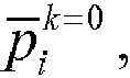


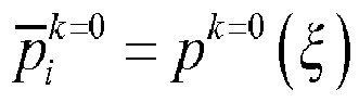


- After solving the pressure equation Equations (15-16), the remaining variables (i.e., saturations and molar fractions) can be recovered from Equations (5-11). It may not be required in the case of FULLIMP, IMPSAT to construct the total velocity field to compute hyperbolic variables.
-
Fig. 1 illustrates an example partial set of actions for performing constrained proposed pressure residual Galerkin multiscale (CPR-GMS) and constrained pressure residual non-Galerkin multiscale (CPR-NGMS) methods. In some embodiments, actions 1-2 and 8-12 can be the same as these shown in the original CPR-type. Actions 3 and 4 can utilize advantages of the multiscale technology as described herein. In a case of monotone method (e.g., MML-CPR-NGMS and MML-CPR-GMS) an algorithm can be applied to obtain final coarse level pressure. Basis functions, needed for the construction of MS restriction [R] and prolongation [P] operators, can be computed at the beginning of each time step or at the beginning of the simulation and kept constant throughout the Newton-Raphson loop or simulation respectively. In addition, the update of basis functions can be done adaptively in some parts of the reservoir. Updating them at the end of each Newton-Raphson iteration may be useful when large time step sizes are used. The coarse system can be solved (action 5) with any of a number of various different strategies. - The choice of the solver for the coarse pressure system may be related to the size of the coarse pressure matrix. This may depend both on the size of the model and on the choice of the coarsening factors. If the size of the coarse system is small enough, a direct solver can be used. For large cases, in order to obtain a small coarse pressure matrix, very large coarsening factors may be used. This may slow down the computation of basis functions as a direct solver is usually used for this action. In order to avoid this slow down, an iterative method may be used for the basis functions computation; in certain embodiments, this occurs at the beginning of the simulation process. Increasing the coarsening factors too much may affect the accuracy of the pressure solution and the number of nonlinear iterations.
- Following the structure of multigrid solver techniques, pre- and post-smoothing actions on the fine scale pressure solution may be introduced. The fine scale pressure solution may be smoothed using, by way of non-limiting example, either Gauss-Seidel (GS) or ILU(0).
- The above can be applied in the case of a reservoir containing miscible three phase black oil. For example, using IMPES formulation, the pressure equations may be solved assuming only SW and SG are fixed. In some embodiments, a coupled system for pressure may be formed (e.g., using pG and Rs for GasWater cell state); see Equation (2). The variables R s may be eliminated by using a Schur complement (it is inexpensive and localized); see Equation (5). The resulting pressure Equations (15-16) matrix may be solved with a multiscale method, and then Rs may be updated together with bG and bO. By doing this operation, the pressure equation (mechanical equilibrium) may feel the changes in the chemical equilibrium and vice versa. This operation is called second stage reduction in the prior art INTERSECT® simulator and it is generally not that expensive. The velocity may be computed using updated variable R s , pG, bO, and bG. The rest of computations may be the same as in the conventional prior art INTERSECT® multiscale implementation.
- This section describes a Multiscale (MS) method for fully implicit simulations of multiphase flow in highly heterogeneous porous media. From a fully implicit Jacobian, a Constrained Pressure Residual (CPR) preconditioning method is used to extract the pressure system. This pressure system is then coupled with a second stage solver for the full residual correction, as it is done in the classical CPR-based fully implicit solvers. Among other innovations, some embodiments employ MsFEM or MsFVM or MsRBS to obtain an approximate solution of the CPR-based pressure system. More precisely, the global solver may be based on a multiscale coarse-scale system (MsFVM or MsFEM or MsRBS), before and after which pre- and post-smoothing may be applied on the fine scale solution in order to eliminate high-frequency errors. This multi-stage multiscale strategy combines the advantages of multiscale methods with the stability of fully implicit systems for highly coupled problems. As such, being integrated in the fully implicit iterative procedure, the CPR-MS captures the strong nonlinear coupling terms efficiently.
- Mathematical formulation of multi-component/multi-phase fluid flow in hydrocarbons reservoirs leads to nonlinear coupled system of partial differential equations (PDEs). To solve the strongly nonlinear and coupled system of discretized equations, arising from the spatial and temporal discretization of the governing equations, a global linearization Newton-Raphson method may be used. This global linearization can result in sparse large linear systems of equations, by way of non-limiting example, represented as follows.

- In Equation (32), J pp is the pressure block coefficients, J ss is the non-pressure block (saturations or components molar fractions) coefficients, J ps and J sp represent the respective coupling coefficients. The terms Δxp and Δxs represent the increments of pressure (primary variables or physical parameters) and of the other (secondary) variables or physical parameters (e.g., saturations and components molar fractions). In many practical scenarios the linear solver action represents a dominant part of the whole computational time. Performance of iterative linear solvers strongly depends on robust and fast preconditioners, amenable for massive parallelization. Additionally, for realistic-scale problems, the memory requirement to store the sparse Jacobian linear systems becomes an important consideration.
- Linear solvers generally used in reservoir simulations consist of preconditioned Krylov subspace methods such as ORTHOMIN with nested factorization as a preconditioner. A significant improvement in preconditioning strategy of linear systems arising from reservoir simulations was made by introducing the Constrained Pressure Residual preconditioning (CPR) method. The CPR preconditioner acknowledges the fact that Equation (32) is of a mixed parabolic (or elliptic)-hyperbolic type. By targeting the parabolic part of the system (or elliptic for incompressible flow) as a separate inner stage, the CPR method improves the convergence rate for the full linear system, based on a pressure predictor-corrector strategy for each linear step. The pressure equation may be constructed by an IMPES-like reduction of Equation (32), discussed above, where both sides are multiplied by a matrix of the form (i.e., Schur complement with the matrix J ss ):

in order to obtain
where

and
In order to simplify the Schur complement procedure, it is assumed that
- where matrices J ps and J ss are replaced by vectors whose elements are the sums of each column. This implies that


- or that the pressure matrix can be extracted as follows

- The effectiveness of CPR methods depends, to a large extent, on the quality of the pressure matrix


- Quasi-IMPES
- True-IMPES
- For Quasi-IMPES scheme, some embodiments ignore the off-diagonal J ps terms and eliminate the diagonal part of J ps using the inverse of the block-diagonal of J ss .
- Equation (36) is the pressure equation. It forms an approximation of the parabolic (or elliptic for incompressible flow) part of the discrete operator and may be considered separately from the remaining hyperbolic part.
-
Fig. 2 is a schematic diagram illustrating a method for flexible generalized minimal residual (FGMRES) preconditioned by a two-stage constrained pressure residual preconditioner. The linear system of Equation (32) (formulation 202) may be solved by flexible generalized minimal residual 208 (FGMRES), preconditioned by theCPR method 210. The preconditioner can include two complementary stages. Thefirst stage 212 may be used to approximate the pressure solution by commonly applying Algebraic Multigrid (AMG) method to Equation (36). In thesecond stage 214, another preconditioner (e.g., the ILU(O) method) may be applied to the full system of Equation (32) such that the first stage pressure approximation is used as the initial guess. Thus,Fig. 2 illustrates the process for a giventime step 204, in which is nested a Newton-Raphson loop 206 withattendant convergence detection 218. - A linear solver based on CPR-AMG preconditioning may be effective in terms of algorithmic efficiency. However, there are still challenges to overcome in implementing a near-ideal scalable AMG solver. Also, the second stage of CPR preconditioning often incudes a variant of an incomplete LU factorization, which again is non-trivial to parallelize. As a result, the linear solver is still some way from near-ideal scalability. In what follows, the Constrained Pressure Residual Multiscale (CPR-MS) Solver is described, embodiments of which address some or all of these shortcomings.
- Analogously to finite element methods, multiscale methods use an approximation space that is spanned by basis functions. Some embodiments use multiscale finite element basis functions to create an approximation space for pressure of much lower dimension than the original simulation grid. The approximation space may be constructed using a discretization for pressure to capture the effect of fine-scale heterogeneity locally.
- In the MsFEM, MsFVM and MsRBS methods, the discretization for pressure basis functions may be obtained from sequential formulation. The pressure residual is formed like in IMPES formulation by eliminating the unknown saturation from the mass balance equations. The pressure matrix may be the Jacobian of the pressure residual.
-
Fig. 3 schematically illustrates a simulation grid with both a fine partition and coarse overlapping subdomains. For the MsFE basis functions, the simulation grid is partitioned into overlappingsubdomains 302, where the cells (e.g., 306) in theoverlap region 308 form a coarse mesh. The MsFV method uses anon-overlapping partition 304. - Let the dual coarse grid be a partition,

- For each subdomain Dk , compute basis functions





- Some embodiments utilize restriction operators R to form a linear system for the pressure in the wirebasket corner cells. Two different restriction operators may be used, by way of non-limiting example. One is to use RFE = P T. The application of RFE to a vector x yields a weighted sum ofx for cells near each wirebasket corner cell. Applied to a linear system, it yields a classical Galerkin type coarse scale approximation.
- The other useful restriction operator is a finite-volume type restriction RFV. For a nonoverlapping decomposition {Ω1, ..., Ω N } of the simulation grid, dual toin the sense that each subdomain Ω i contains one (and only one) wirebasket corner cell, the RFV may be defined bv


-
Fig. 4 is a schematic diagram illustrating constrained proposed pressure residual Galerkin multiscale (CPR-GMS) and constrained pressure residual non-Galerkin multiscale (CPR-NGMS) methods.Blocks blocks Fig. 2 . - Regarding
blocks Fig. 4 , the CPR-MS algorithm combines both actions of the CPR-AMG method and of multiscale methods. In fact, a fully implicit system may be solved with a CPR type 2-stage preconditioners where a MS method is used for solving the pressure system extracted by the CPR decoupling operator. Starting from the Jacobian matrix J built with a fully implicit formulation, the whole solution strategy can be summarized as follows (the below actions are referred to herein as the "Example Process Summary"). - 1. CPR preconditioning: the pressure matrix is extracted A cpr = C T MJC and the residual is restricted to a pressure residual rp = C Tr. (This action may correspond to
action 2 ofFig. 1 .) - 2. Construction of the coarse pressure system using Restriction (R) and Prolongation (P) operators built with the basis functions computed either with a finite element or finite volume multiscale method:


Fig. 1 .) - 3. The coarse pressure system is solved and its solution is prolongated to the fine scale:


Fig. 1 .) - 4. The full system residual is corrected using the fine scale solution: r* = r-J·(C· Δxp ). (This corresponds to action 8 of
Fig. 1 .) - 5. The corrected full system is solved with a second stage preconditioner: Ax* = M-1 · r*. (This corresponds to action 9 of
Fig. 1 .) - 6. The two solutions are combined in order to build the full system solution: Δx = Δx* + C · Δxp. (This corresponds to action 10 of
Fig. 1 .) -
Actions Actions 2 and 3 may be performed as in typical multiscale methods (block 414 ofFig. 4 ). Thus, the original two-stage preconditioning structure of the solution strategy may be altered to utilize a different choice for the solution of the pressure system. - Basis functions, used for the construction of MS restriction (R) and prolongation (P) operators, may be computed at the beginning of each time step and kept constant throughout the Newton-Raphson loop. Updating them at the end of each Newton-Raphson iteration may be useful when large time step sizes are used.
- The coarse system can be solved (action 3 of the above Example Process Summary) with different strategies. The choice of the solver for the coarse pressure system is strictly related to the size of the coarse pressure matrix; this depends both on the size of the model and on the choice of the coarsening factors. If the size of the coarse system is small enough a direct solver can be used; for big cases, in order to obtain a small coarse pressure matrix, very large coarsening factors may be used. This may slow down the computation of basis functions because a direct solver is usually used for this action; in order to avoid this slow down, an iterative method may be used for the basis functions computation. The advantage of doing that is that basis functions calculation is only done once per each time step, whereas a different coarse system may be solved for each Newton iteration. However, increasing too much the coarsening factors may affect the accuracy of our pressure solution and the number of nonlinear iterations may grow.
- Following the structure of a multigrid solver, pre- and post-smoothing actions (
blocks -
Fig. 5 illustrates an example reservoir representation depicting a fine grid of 648,000 cells. That is,Fig. 5 depicts a fine grid utilized for the test case. Thegrid 502 was 144 × 150 × 30, for a total of 648,000 cells. - Results and performance were compared with the current version of the INTERSECT® (IX) simulator, which uses CPR preconditioning with a IV-cycle AMG for solving the pressure system and ILU(0) as a second stage preconditioner. Thus, the solution obtained with the current version of IX was used as a reference. The same second stage preconditioner was used so that the only difference is solution strategy of the pressure system. Two different values for the minimum time step size were used which resulted in two completely different time step selections throughout the simulation. The maximum time step size was always kept the same.
- All results presented were obtained in serial runs. The algorithm is highly parallelizable and its potential is even greater for parallel runs.
- For the first set of runs, a minimum time step size of 15 days was used. Finite element (FE) basis functions were used. The coarsening factors for the three directions were (3,5,5), which resulted in a coarse grid of 48 × 30 × 6, for a total of 8,640 cells. With such a size of the coarse pressure matrix, direct methods are very slow. For this reason, no results are presented for runs which use a direct solver on the coarse pressure system.
Table 1 Settings of all runs for a minimum time step size of 15 days Runs Pre-smoothing Post-smoothing Coarse Solver Run 1 GS GS AMG Run 2 GS GS GMRES-AMG Run 3 GS GS AMG Run 4 none GS AMG - Before proceeding with the analysis of the performance in terms of number of linear iterations and CPU time of the CPR-MS solver, it is important to make sure that the solution does not change. All computed results appeared to be exactly identical to the reference solution, as shown in
Fig. 6 . -
Fig. 6 illustrates graphs depicting field pressure and gas block saturation solutions for CPR-AMG and CPR-MS.Graph 602 depicts average pressure of the entire reservoir.Graph 604 depicts a gas saturation profile of a particular location, (120.65, 1). As depicted inFig. 6 , the two solutions completely match; no exceptions to complete overlap of the curves are visible inFig. 6 , in eithergraph - Table 2, below, depicts the results in terms of performance (number of iterations and CPU time) for the four performed runs and for the current INTERSECT configuration (CPR-AMG).
Table 2 Results of all runs for a minimum time step size of 15 days Number of iterations CPU time (s) Runs Non linear iter. Linear iter. Linear Solver total Run 1 369 2872 1615 2699 Run 2369 2845 1119 2203 Run 3 371 3327 1233 2309 Run 4 371 3649 2026 3114 IX 369 2187 1571 2537 - In the test runs, the number of non-linear iterations was almost constant. For Run 3 and Run 4, the heuristic functionality was used; it keeps AMG restriction and prolongation operators constant for a certain number of iterations allowing a speed up of the set-up phase of the AMG solver.
- The CPR-MS algorithm uses a greater number of linear iterations than the original Intersect CPR-AMG; this was actually expected as MS methods usually require a great number of linear iterations. Pre and post-smoothing help limiting the growth in the number of linear iterations.
- The following table summarizes the relative difference in CPU time between each run and the reference Intersect CPR-AMG run.
Table 3
Runs Δ % Run 1 +6.38 Run 2 -13.17 Run 3 -8.99 Run 4 +22.74 - Comparing the results of Runs 3 and 4, notice that introducing a pre-smoothing reduces considerably the number of linear iterations, and it allows a substantial speedup. Based on these results, using a three-iteration GMRES cycle plus AMG appears to be the most effective choice. If the correct settings are chosen, CPR-MS results to be more than 10% faster than CPR-AMG
- For the second set of runs a minimum time step size of one day was used. This was the only difference between the two sets of runs. In fact, the same coarsening factors and FE restriction and prolongation operators were used. Heuristic was used for runs 8 and 9.
Table 4 Settings of all runs for a minimum time step size of 1 day Runs Pre-smoothing Post-smoothing Coarse Solver Run 6 GS GS GMRES-AMG Run 7 none GS AMG Run 8 none GS AMG Run 9 GS GS AMG - Even for this set of runs, the CPR-MS solver solutions perfectly match the ones provided by Intersect.
Table 5 Results of all runs for a minimum time step size of 1 day Number of iterations CPU time (s) Runs Non linear iter. Linear iter. Linear Solver total Run 6 711 4210 1718 3887 Run 7 709 4804 3301 5576 Run 8 708 5254 1911 4085 Run 9 709 4658 3212 5472 IX 706 2868 2718 4666 - The number of linear iterations for CPR-MS is greater than the one of CPR-AMG. Results for the smaller times step size seem to confirm what was observed for the bigger one.
Table 6
Runs Δ% Run 6 -16.69 Run 7 +19.5 Run 8 -12.45 Run 9 + 17.27 - Although, using a pre-smoothing in this case does not seem to be as effective as in the previous one; in fact, by comparing runs 8 and 9, in which the only difference is the presence of the pre-smoother, using a pre-smoother slows down the simulation instead of speeding it up. A GMRES solver preconditioned by AMG appears to be efficient for the coarse pressure system solver in some scenarios.
-
Fig. 7 is a flowchart depicting a method according to some embodiments. The method may be implemented using hardware specialized for parallel processing, such as that described below in reference toFig. 8 . The method may be applied obtain solutions to a linear system of equations arising from the linearization of coupled nonlinear hyperbolic / parabolic (elliptic) partial differential equations (PDEs) of fluid flow in heterogeneous anisotropic porous media. More generally, the method may be applied model the behavior of a petroleum reservoir. - At
block 702, the method obtains measurements of physical parameters of the reservoir at various locations within the reservoir and at various times. The number of measurements can range from hundreds to billions. The measured physical parameters can include pressure, phase saturations and phase-specific molar fractions, e.g., as described above in Section I. Various techniques may be utilized to obtain such measurements, such as the use of down-hole sensors. - At
block 704, the method discretizes a system of partial differential equations that are formed according to the measurements obtained atblock 702. More particularly, the method may form a system of partial differential equations as described above in reference to Equations (1-3) generally, or, more particularly, Equations (4-7). The discretization technique applied to such a system of equations may include, by way of non-limiting example, a finite-volume, second-order state, first-order time technique. More generally, the system of partial differential equations may be discretized using techniques described above in reference to Equation (8). - At
block 706, the method establishes one or more nested loops for processing at each of a plurality of time steps and each of a plurality of physical parameter values. Such nested loops are depicted graphically in, and described in reference to,Figs. 2 and4 , for example. The outer loop may iterate per time step, while the inner loop may perform iterations of the Newton-Raphson technique. Each Newton-Raphson iteration may compute a solution to Equation (9) using Equations (10-14), for example. - Note that the processes within the nested loops may be parallelized in computer hardware in order to improve performance. That is, implementations of the invention are particularly suited to execution on parallel processing hardware. To that end, Graphical Processing Units (GPUs) may be used to handle the processing within the nested loops at least partially in parallel.
- At
block 708, the method approximates a rough solution (initial guess), e.g., to Equation (9) for the time step currently being processed. The technique may utilize a preconditioning process as described herein. The solution from the previous time step may be assumed as initial guess. - At
block 709, the method updates the residuals. The actions of this block may be performed as is implicit in action 3 ofFig. 1 . (Note that the actions of this block are distinct from action 8 ofFig. 1 .) - At
block 710, the method extracts a system of linear equations representing pressure. The actions of this block may be performed as described herein in reference to Equations (15-20),action 2 ofFig. 2 , block 410 ofFig. 4 , andaction 1 of the Example Process Summary. More generally, the actions of this block correspond to at least part of the Constrained Pressure Residual (CPR) technique described herein. - At
block 712, the method applies a pre-smoothing technique. The actions of this block may be performed as described herein in reference to action 3 ofFig. 1 , and block 412 ofFig. 4 . - At
block 714, the method applies multi-scale multi-level processing. The actions of this block may be performed as described herein in reference to Equations (21-28), action 3 of the Example Process Summary, actions 4-6 ofFig. 1 , and block 414 ofFig. 4 . - At
block 716, the method applies a post-smoothing technique. The actions of this block may be performed as described herein in reference to action 7 ofFig. 1 , and block 416 ofFig. 4 . - At
block 718, having obtained pressure value(s), the method solves for the remaining physical parameters. The actions of this block may be performed as described herein in reference to action 6 of the Example Process Summary, andactions 10 and 11 ofFig. 1 . - At
block 720, the technique determines whether to repeat the iteration(s) initiated atblock 706. This may include determining whether the Newton-Raphson technique has sufficiently converged. The actions of this block may be performed as described herein in reference toaction 12 ofFig. 1 , and block 418 ofFig. 4 . - At
block 722, the method outputs the solution. The outputting may take on various forms. The outputting may include displaying a pictorial representation of all or part of the reservoir, displaying one or more graphs depicting one or more physical parameters, delivering data to a separate process (e.g., to determine whether to extract petroleum), or other outputting techniques. -
Fig. 8 illustrates a schematic view of a computing orprocessor system 800, according to an embodiment. Theprocessor system 800 may include one ormore processors 802 of varying core configurations (including multiple cores) and clock frequencies. The one ormore processors 802 may be operable to execute instructions, apply logic, etc. It will be appreciated that these functions may be provided by multiple processors or multiple cores on a single chip operating in parallel and/or communicably linked together. In at least one embodiment, the one ormore processors 802 may be or include one or more GPUs. - The
processor system 800 may also include a memory system, which may be or include one or more memory devices and/or computer-readable media 804 of varying physical dimensions, accessibility, storage capacities, etc. such as flash drives, hard drives, disks, random access memory, etc., for storing data, such as images, files, and program instructions for execution by theprocessor 802. In an embodiment, the computer-readable media 804 may store instructions that, when executed by theprocessor 802, are configured to cause theprocessor system 800 to perform operations. For example, execution of such instructions may cause theprocessor system 800 to implement one or more portions and/or embodiments of the methods described herein. - The
processor system 800 may also include one or more network interfaces 806. The network interfaces 806 may include any hardware, applications, and/or other software. Accordingly, the network interfaces 806 may include Ethernet adapters, wireless transceivers, PCI interfaces, and/or serial network components, for communicating over wired or wireless media using protocols, such as Ethernet, wireless Ethernet, etc. - The
processor system 800 may further include one or moreperipheral interfaces 808, for communication with a display screen, projector, keyboards, mice, touchpads, sensors, other types of input and/or output peripherals, and/or the like. In some implementations, the components ofprocessor system 800 need not be enclosed within a single enclosure or even located in close proximity to one another, but in other implementations, the components and/or others may be provided in a single enclosure. - The
memory device 804 may be physically or logically arranged or configured to store data on one ormore storage devices 810. Thestorage device 810 may include one or more file systems or databases in any suitable format. Thestorage device 810 may also include one ormore software programs 812, which may contain interpretable or executable instructions for performing one or more of the disclosed processes. When requested by theprocessor 802, one or more of thesoftware programs 812, or a portion thereof, may be loaded from thestorage devices 810 to thememory devices 804 for execution by theprocessor 802. - Those skilled in the art will appreciate that the above-described componentry is merely hardware components, including any necessary accompanying firmware or software, for performing the disclosed implementations. The
processor system 800 may also be implemented in part or in whole by electronic circuit components or processors, such as application-specific integrated circuits (ASICs) or field-programmable gate arrays (FPGAs). - The actions described need not be performed in the same sequence discussed or with the same degree of separation. Various actions may be omitted, repeated, combined, or divided, as necessary to achieve the same or similar objectives or enhancements. Accordingly, the present disclosure is not limited to the above-described embodiments, but instead is defined by the appended claims in light of their full scope of equivalents. Further, in the above description and in the below claims, unless specified otherwise, the term "execute" and its variants are to be interpreted as pertaining to any operation of program code or instructions on a device, whether compiled, interpreted, or run using other techniques.

Claims (15)
- A computer-implemented method for modeling behavior of at least one fluid in a reservoir, the method comprising:obtaining a plurality of measurements of a plurality of physical parameters at a plurality of locations within the reservoir, the plurality of physical parameters comprising at least pressure;discretizing a system of partial differential equations that model, based on the plurality of measurements, the plurality of physical parameters;iterating, for each of a plurality of time steps, and until convergence upon a solution to the system of partial differential equations:approximating a rough solution to the system of partial differential equations;applying a constrained pressure residual technique to extract a system of pressure linear equations from the rough solution to the system of partial differential equations;applying a pre-smoothing technique at a fine scale to determine an approximate solution to the system of pressure linear equations;applying multi-scale multi-level processing to improve the approximate solution to the system of pressure linear equations;applying a post-smoothing technique at a fine scale to further improve the approximate solution to the system of pressure linear equations; andsolving the system of partial differential equations for remaining physical parameters based on the further improved approximate solution to the system of pressure linear equations; andoutputting the solution to the system of partial differential equations.
- The method of claim 1, wherein the outputting comprises displaying a representation of a behavior of the at least one fluid in the reservoir.
- The method of claim 1, further comprising:predicting fluid behavior in the reservoir based on the system of partial differential equations; andextracting fluid from the reservoir based on the predicting.
- The method of claim 1, wherein the iterating is performed in parallel by at least one hardware graphics processing unit.
- The method of claim 1, further comprising history matching the system of partial differential equations.
- The method of claim 1, wherein the physical parameters comprise pressure, flow rate, and composition.
- The method of claim 1, wherein the reservoir comprises heterogeneous anisotropic porous media.
- The method of claim 1, wherein at least one of the applying a pre-smoothing technique and the applying a post-smoothing technique comprises applying at least one technique selected from the group consisting of: applying ILU(0), applying a Jacobi smoother, and applying a Gauss-Seidel smoother.
- A computer system for modeling behavior of at least one fluid in a reservoir, the system comprising at least one electronic processor and persistent memory storing computer-interpretable instructions configured to cause the at least one processor to perform a method comprising:obtaining a plurality of measurements of a plurality of physical parameters at a plurality of locations within the reservoir, the plurality of physical parameters comprising at least pressure;discretizing a system of partial differential equations that model, based on the plurality of measurements, the plurality of physical parameters;iterating, for each of a plurality of time steps, and until convergence upon a solution to the system of partial differential equations:approximating a rough solution to the system of partial differential equations;applying a constrained pressure residual technique to extract a system of pressure linear equations from the rough solution to the system of partial differential equations;applying a pre-smoothing technique at a fine scale to determine an approximate solution to the system of pressure linear equations;applying multi-scale multi-level processing to improve the approximate solution to the system of pressure linear equations;applying a post-smoothing technique at a fine scale to further improve the approximate solution to the system of pressure linear equations; andsolving the system of partial differential equations for remaining physical parameters based on the further improved approximate solution to the system of pressure linear equations; andoutputting the solution to the system of partial differential equations.
- The system of claim 9, wherein the outputting comprises displaying a representation of a behavior of the at least one fluid in the reservoir.
- The system of claim 9, wherein the instructions are further configured to cause the at least one processor to perform:predicting fluid behavior in the reservoir based on the system of partial differential equations; andextracting fluid from the reservoir based on the predicting.
- The system of claim 9 further comprising at least one graphics processing unit, wherein the iterating is performed in parallel by the at least one hardware graphics processing unit.
- The system of claim 9 wherein the instructions are further configured to cause the at least one processor to perform history matching the system of partial differential equations.
- The system of claim 9, wherein the physical parameters comprise pressure, flow rate, and composition.
- The system of claim 9, wherein the reservoir comprises heterogeneous anisotropic porous media.
Applications Claiming Priority (1)
| Application Number | Priority Date | Filing Date | Title |
|---|---|---|---|
| US201462018318P | 2014-06-27 | 2014-06-27 |
Publications (3)
| Publication Number | Publication Date |
|---|---|
| EP2960430A2 true EP2960430A2 (en) | 2015-12-30 |
| EP2960430A3 EP2960430A3 (en) | 2016-04-27 |
| EP2960430B1 EP2960430B1 (en) | 2017-08-09 |
Family
ID=53541513
Family Applications (1)
| Application Number | Title | Priority Date | Filing Date |
|---|---|---|---|
| EP15174003.2A Active EP2960430B1 (en) | 2014-06-27 | 2015-06-26 | Multilevel monotone constrained pressure residual multiscale techniques |
Country Status (3)
| Country | Link |
|---|---|
| US (1) | US20160162612A1 (en) |
| EP (1) | EP2960430B1 (en) |
| NO (1) | NO3133073T3 (en) |
Cited By (2)
| Publication number | Priority date | Publication date | Assignee | Title |
|---|---|---|---|---|
| WO2020068442A1 (en) * | 2018-09-24 | 2020-04-02 | Saudi Arabian Oil Company | Reservoir simulation with pressure solver for non-diagonally dominant indefinite coefficient matrices |
| US12497887B2 (en) | 2021-10-20 | 2025-12-16 | Chevron U.S.A. Inc. | Acceleration of subsurface simulation using filtered grid connectivity graph |
Families Citing this family (3)
| Publication number | Priority date | Publication date | Assignee | Title |
|---|---|---|---|---|
| US11543560B2 (en) * | 2018-04-13 | 2023-01-03 | Schlumberger Technology Corporation | Method for reservoir simulation optimization under geological uncertainty |
| CN118551939B (en) * | 2024-07-23 | 2024-11-05 | 广东翔晟箱配科技有限公司 | Intelligent monitoring method and system for the whole process of luggage accessories production |
| CN120495444B (en) * | 2025-04-29 | 2025-12-16 | 中国矿业大学(北京) | Geological modeling method and related device based on self-adaptive geometric multiple grids |
Family Cites Families (5)
| Publication number | Priority date | Publication date | Assignee | Title |
|---|---|---|---|---|
| EA201270601A1 (en) * | 2009-10-28 | 2012-11-30 | Шеврон Ю.Эс.Эй. Инк. | MULTI-SCALE METHOD OF FINAL VOLUMES FOR MODELING COLLECTORS |
| US8798977B2 (en) * | 2010-12-16 | 2014-08-05 | Chevron U.S.A. Inc. | System and method for simulating fluid flow in a fractured reservoir |
| GB2506271A (en) * | 2012-08-10 | 2014-03-26 | Schlumberger Holdings | Modeling a fractured medium |
| US20140136171A1 (en) * | 2012-11-13 | 2014-05-15 | Chevron U.S.A. Inc. | Unstructured Grids For Modeling Reservoirs |
| US9790770B2 (en) * | 2013-10-30 | 2017-10-17 | The Texas A&M University System | Determining performance data for hydrocarbon reservoirs using diffusive time of flight as the spatial coordinate |
-
2013
- 2013-01-03 NO NO16189661A patent/NO3133073T3/no unknown
-
2015
- 2015-06-26 EP EP15174003.2A patent/EP2960430B1/en active Active
- 2015-06-26 US US14/751,736 patent/US20160162612A1/en not_active Abandoned
Non-Patent Citations (1)
| Title |
|---|
| None |
Cited By (6)
| Publication number | Priority date | Publication date | Assignee | Title |
|---|---|---|---|---|
| WO2020068442A1 (en) * | 2018-09-24 | 2020-04-02 | Saudi Arabian Oil Company | Reservoir simulation with pressure solver for non-diagonally dominant indefinite coefficient matrices |
| CN112752894A (en) * | 2018-09-24 | 2021-05-04 | 沙特阿拉伯石油公司 | Reservoir simulation with pressure solver for non-diagonally dominant indeterminate coefficient matrix |
| JP2021534517A (en) * | 2018-09-24 | 2021-12-09 | サウジ アラビアン オイル カンパニー | Reservoir simulation with pressure solver for off-diagonal dominant indefinite coefficient matrix |
| US11461514B2 (en) | 2018-09-24 | 2022-10-04 | Saudi Arabian Oil Company | Reservoir simulation with pressure solver for non-diagonally dominant indefinite coefficient matrices |
| CN112752894B (en) * | 2018-09-24 | 2023-02-28 | 沙特阿拉伯石油公司 | Reservoir simulation with pressure solver for non-diagonally dominant indeterminate coefficient matrix |
| US12497887B2 (en) | 2021-10-20 | 2025-12-16 | Chevron U.S.A. Inc. | Acceleration of subsurface simulation using filtered grid connectivity graph |
Also Published As
| Publication number | Publication date |
|---|---|
| NO3133073T3 (en) | 2018-09-29 |
| EP2960430A3 (en) | 2016-04-27 |
| US20160162612A1 (en) | 2016-06-09 |
| EP2960430B1 (en) | 2017-08-09 |
Similar Documents
| Publication | Publication Date | Title |
|---|---|---|
| Klawonn et al. | Toward extremely scalable nonlinear domain decomposition methods for elliptic partial differential equations | |
| Kippe et al. | A comparison of multiscale methods for elliptic problems in porous media flow | |
| Zhou et al. | Operator-based multiscale method for compressible flow | |
| Stüben et al. | Algebraic multigrid methods (AMG) for the efficient solution of fully implicit formulations in reservoir simulation | |
| US8346523B2 (en) | Indirect-error-based, dynamic upscaling of multi-phase flow in porous media | |
| US20130085730A1 (en) | Preconditioner for reservoir simulation | |
| EP2960430B1 (en) | Multilevel monotone constrained pressure residual multiscale techniques | |
| MacLachlan et al. | Local Fourier analysis for multigrid with overlapping smoothers applied to systems of PDEs | |
| US10534877B2 (en) | Adaptive multiscale multi-fidelity reservoir simulation | |
| EP2756382A1 (en) | Optimized matrix and vector operations in instruction limited algorithms that perform eos calculations | |
| Chiocchetti et al. | An exactly curl-free staggered semi-implicit finite volume scheme for a first order hyperbolic model of viscous two-phase flows with surface tension | |
| Gries | On the convergence of system-AMG in reservoir simulation | |
| Brubeck et al. | Multigrid solvers for the de Rham complex with optimal complexity in polynomial degree | |
| Ngondiep | An efficient high‐order two‐level explicit/implicit numerical scheme for two‐dimensional time fractional mobile/immobile advection‐dispersion model | |
| Modares et al. | Dynamic analysis of structures with interval uncertainty | |
| Montoya et al. | Efficient tensor-product spectral-element operators with the summation-by-parts property on curved triangles and tetrahedra | |
| Fu et al. | An adaptive preconditioner for three-dimensional single-phase compressible flow in highly heterogeneous porous media | |
| Konshin et al. | Distributed parallel bootstrap adaptive algebraic multigrid method | |
| Müller et al. | Parallel multilevel Monte Carlo for two-phase flow and transport in random heterogeneous porous media with sampling-error and discretization-error balancing | |
| Suarez et al. | A method for solving the molecular Schrödinger equation in Cartesian coordinates via angular momentum projection operators | |
| Negrello et al. | A new impedance accounting for short‐and long‐range effects in mixed substructured formulations of nonlinear problems | |
| US20200325765A1 (en) | Method and device for determining hydrocarbon production for a reservoir | |
| Yang et al. | Multiscale hybridizable discontinuous Galerkin method for flow simulations in highly heterogeneous media | |
| Carvalho et al. | Speeding up parallel performance of porous media flow simulations using multiscale preconditioners | |
| Bergamaschi et al. | Parallel RFSAI‐BFGS preconditioners for large symmetric eigenproblems |
Legal Events
| Date | Code | Title | Description |
|---|---|---|---|
| PUAI | Public reference made under article 153(3) epc to a published international application that has entered the european phase |
Free format text: ORIGINAL CODE: 0009012 |
|
| 17P | Request for examination filed |
Effective date: 20150626 |
|
| AK | Designated contracting states |
Kind code of ref document: A2 Designated state(s): AL AT BE BG CH CY CZ DE DK EE ES FI FR GB GR HR HU IE IS IT LI LT LU LV MC MK MT NL NO PL PT RO RS SE SI SK SM TR |
|
| AX | Request for extension of the european patent |
Extension state: BA ME |
|
| PUAL | Search report despatched |
Free format text: ORIGINAL CODE: 0009013 |
|
| AK | Designated contracting states |
Kind code of ref document: A3 Designated state(s): AL AT BE BG CH CY CZ DE DK EE ES FI FR GB GR HR HU IE IS IT LI LT LU LV MC MK MT NL NO PL PT RO RS SE SI SK SM TR |
|
| AX | Request for extension of the european patent |
Extension state: BA ME |
|
| RIC1 | Information provided on ipc code assigned before grant |
Ipc: E21B 49/00 20060101AFI20160318BHEP |
|
| GRAP | Despatch of communication of intention to grant a patent |
Free format text: ORIGINAL CODE: EPIDOSNIGR1 |
|
| INTG | Intention to grant announced |
Effective date: 20170516 |
|
| RIN1 | Information on inventor provided before grant (corrected) |
Inventor name: NATVIG, JOSTEIN Inventor name: BRATVEDT, KYRRE Inventor name: HAJIBEYGI, HADI Inventor name: LUKYANOV, ALEXANDER |
|
| GRAS | Grant fee paid |
Free format text: ORIGINAL CODE: EPIDOSNIGR3 |
|
| GRAA | (expected) grant |
Free format text: ORIGINAL CODE: 0009210 |
|
| AK | Designated contracting states |
Kind code of ref document: B1 Designated state(s): AL AT BE BG CH CY CZ DE DK EE ES FI FR GB GR HR HU IE IS IT LI LT LU LV MC MK MT NL NO PL PT RO RS SE SI SK SM TR |
|
| REG | Reference to a national code |
Ref country code: GB Ref legal event code: FG4D |
|
| REG | Reference to a national code |
Ref country code: CH Ref legal event code: EP Ref country code: AT Ref legal event code: REF Ref document number: 917074 Country of ref document: AT Kind code of ref document: T Effective date: 20170815 |
|
| REG | Reference to a national code |
Ref country code: IE Ref legal event code: FG4D |
|
| REG | Reference to a national code |
Ref country code: DE Ref legal event code: R096 Ref document number: 602015003981 Country of ref document: DE |
|
| REG | Reference to a national code |
Ref country code: NL Ref legal event code: MP Effective date: 20170809 |
|
| REG | Reference to a national code |
Ref country code: LT Ref legal event code: MG4D |
|
| REG | Reference to a national code |
Ref country code: AT Ref legal event code: MK05 Ref document number: 917074 Country of ref document: AT Kind code of ref document: T Effective date: 20170809 |
|
| REG | Reference to a national code |
Ref country code: NO Ref legal event code: T2 Effective date: 20170809 |
|
| PG25 | Lapsed in a contracting state [announced via postgrant information from national office to epo] |
Ref country code: AT Free format text: LAPSE BECAUSE OF FAILURE TO SUBMIT A TRANSLATION OF THE DESCRIPTION OR TO PAY THE FEE WITHIN THE PRESCRIBED TIME-LIMIT Effective date: 20170809 Ref country code: FI Free format text: LAPSE BECAUSE OF FAILURE TO SUBMIT A TRANSLATION OF THE DESCRIPTION OR TO PAY THE FEE WITHIN THE PRESCRIBED TIME-LIMIT Effective date: 20170809 Ref country code: HR Free format text: LAPSE BECAUSE OF FAILURE TO SUBMIT A TRANSLATION OF THE DESCRIPTION OR TO PAY THE FEE WITHIN THE PRESCRIBED TIME-LIMIT Effective date: 20170809 Ref country code: LT Free format text: LAPSE BECAUSE OF FAILURE TO SUBMIT A TRANSLATION OF THE DESCRIPTION OR TO PAY THE FEE WITHIN THE PRESCRIBED TIME-LIMIT Effective date: 20170809 Ref country code: NL Free format text: LAPSE BECAUSE OF FAILURE TO SUBMIT A TRANSLATION OF THE DESCRIPTION OR TO PAY THE FEE WITHIN THE PRESCRIBED TIME-LIMIT Effective date: 20170809 Ref country code: SE Free format text: LAPSE BECAUSE OF FAILURE TO SUBMIT A TRANSLATION OF THE DESCRIPTION OR TO PAY THE FEE WITHIN THE PRESCRIBED TIME-LIMIT Effective date: 20170809 |
|
| PG25 | Lapsed in a contracting state [announced via postgrant information from national office to epo] |
Ref country code: LV Free format text: LAPSE BECAUSE OF FAILURE TO SUBMIT A TRANSLATION OF THE DESCRIPTION OR TO PAY THE FEE WITHIN THE PRESCRIBED TIME-LIMIT Effective date: 20170809 Ref country code: BG Free format text: LAPSE BECAUSE OF FAILURE TO SUBMIT A TRANSLATION OF THE DESCRIPTION OR TO PAY THE FEE WITHIN THE PRESCRIBED TIME-LIMIT Effective date: 20171109 Ref country code: RS Free format text: LAPSE BECAUSE OF FAILURE TO SUBMIT A TRANSLATION OF THE DESCRIPTION OR TO PAY THE FEE WITHIN THE PRESCRIBED TIME-LIMIT Effective date: 20170809 Ref country code: PL Free format text: LAPSE BECAUSE OF FAILURE TO SUBMIT A TRANSLATION OF THE DESCRIPTION OR TO PAY THE FEE WITHIN THE PRESCRIBED TIME-LIMIT Effective date: 20170809 Ref country code: ES Free format text: LAPSE BECAUSE OF FAILURE TO SUBMIT A TRANSLATION OF THE DESCRIPTION OR TO PAY THE FEE WITHIN THE PRESCRIBED TIME-LIMIT Effective date: 20170809 Ref country code: IS Free format text: LAPSE BECAUSE OF FAILURE TO SUBMIT A TRANSLATION OF THE DESCRIPTION OR TO PAY THE FEE WITHIN THE PRESCRIBED TIME-LIMIT Effective date: 20171209 Ref country code: GR Free format text: LAPSE BECAUSE OF FAILURE TO SUBMIT A TRANSLATION OF THE DESCRIPTION OR TO PAY THE FEE WITHIN THE PRESCRIBED TIME-LIMIT Effective date: 20171110 |
|
| PG25 | Lapsed in a contracting state [announced via postgrant information from national office to epo] |
Ref country code: RO Free format text: LAPSE BECAUSE OF FAILURE TO SUBMIT A TRANSLATION OF THE DESCRIPTION OR TO PAY THE FEE WITHIN THE PRESCRIBED TIME-LIMIT Effective date: 20170809 Ref country code: CZ Free format text: LAPSE BECAUSE OF FAILURE TO SUBMIT A TRANSLATION OF THE DESCRIPTION OR TO PAY THE FEE WITHIN THE PRESCRIBED TIME-LIMIT Effective date: 20170809 Ref country code: DK Free format text: LAPSE BECAUSE OF FAILURE TO SUBMIT A TRANSLATION OF THE DESCRIPTION OR TO PAY THE FEE WITHIN THE PRESCRIBED TIME-LIMIT Effective date: 20170809 |
|
| REG | Reference to a national code |
Ref country code: DE Ref legal event code: R097 Ref document number: 602015003981 Country of ref document: DE |
|
| PG25 | Lapsed in a contracting state [announced via postgrant information from national office to epo] |
Ref country code: SM Free format text: LAPSE BECAUSE OF FAILURE TO SUBMIT A TRANSLATION OF THE DESCRIPTION OR TO PAY THE FEE WITHIN THE PRESCRIBED TIME-LIMIT Effective date: 20170809 Ref country code: IT Free format text: LAPSE BECAUSE OF FAILURE TO SUBMIT A TRANSLATION OF THE DESCRIPTION OR TO PAY THE FEE WITHIN THE PRESCRIBED TIME-LIMIT Effective date: 20170809 Ref country code: EE Free format text: LAPSE BECAUSE OF FAILURE TO SUBMIT A TRANSLATION OF THE DESCRIPTION OR TO PAY THE FEE WITHIN THE PRESCRIBED TIME-LIMIT Effective date: 20170809 Ref country code: SK Free format text: LAPSE BECAUSE OF FAILURE TO SUBMIT A TRANSLATION OF THE DESCRIPTION OR TO PAY THE FEE WITHIN THE PRESCRIBED TIME-LIMIT Effective date: 20170809 |
|
| PLBE | No opposition filed within time limit |
Free format text: ORIGINAL CODE: 0009261 |
|
| STAA | Information on the status of an ep patent application or granted ep patent |
Free format text: STATUS: NO OPPOSITION FILED WITHIN TIME LIMIT |
|
| REG | Reference to a national code |
Ref country code: FR Ref legal event code: PLFP Year of fee payment: 4 |
|
| 26N | No opposition filed |
Effective date: 20180511 |
|
| PG25 | Lapsed in a contracting state [announced via postgrant information from national office to epo] |
Ref country code: SI Free format text: LAPSE BECAUSE OF FAILURE TO SUBMIT A TRANSLATION OF THE DESCRIPTION OR TO PAY THE FEE WITHIN THE PRESCRIBED TIME-LIMIT Effective date: 20170809 |
|
| REG | Reference to a national code |
Ref country code: DE Ref legal event code: R119 Ref document number: 602015003981 Country of ref document: DE |
|
| REG | Reference to a national code |
Ref country code: CH Ref legal event code: PL |
|
| REG | Reference to a national code |
Ref country code: BE Ref legal event code: MM Effective date: 20180630 |
|
| REG | Reference to a national code |
Ref country code: IE Ref legal event code: MM4A |
|
| PG25 | Lapsed in a contracting state [announced via postgrant information from national office to epo] |
Ref country code: MC Free format text: LAPSE BECAUSE OF FAILURE TO SUBMIT A TRANSLATION OF THE DESCRIPTION OR TO PAY THE FEE WITHIN THE PRESCRIBED TIME-LIMIT Effective date: 20170809 Ref country code: LU Free format text: LAPSE BECAUSE OF NON-PAYMENT OF DUE FEES Effective date: 20180626 |
|
| PG25 | Lapsed in a contracting state [announced via postgrant information from national office to epo] |
Ref country code: IE Free format text: LAPSE BECAUSE OF NON-PAYMENT OF DUE FEES Effective date: 20180626 Ref country code: DE Free format text: LAPSE BECAUSE OF NON-PAYMENT OF DUE FEES Effective date: 20190101 Ref country code: CH Free format text: LAPSE BECAUSE OF NON-PAYMENT OF DUE FEES Effective date: 20180630 Ref country code: LI Free format text: LAPSE BECAUSE OF NON-PAYMENT OF DUE FEES Effective date: 20180630 |
|
| PG25 | Lapsed in a contracting state [announced via postgrant information from national office to epo] |
Ref country code: BE Free format text: LAPSE BECAUSE OF NON-PAYMENT OF DUE FEES Effective date: 20180630 |
|
| PG25 | Lapsed in a contracting state [announced via postgrant information from national office to epo] |
Ref country code: MT Free format text: LAPSE BECAUSE OF NON-PAYMENT OF DUE FEES Effective date: 20180626 |
|
| PG25 | Lapsed in a contracting state [announced via postgrant information from national office to epo] |
Ref country code: TR Free format text: LAPSE BECAUSE OF FAILURE TO SUBMIT A TRANSLATION OF THE DESCRIPTION OR TO PAY THE FEE WITHIN THE PRESCRIBED TIME-LIMIT Effective date: 20170809 |
|
| PG25 | Lapsed in a contracting state [announced via postgrant information from national office to epo] |
Ref country code: PT Free format text: LAPSE BECAUSE OF FAILURE TO SUBMIT A TRANSLATION OF THE DESCRIPTION OR TO PAY THE FEE WITHIN THE PRESCRIBED TIME-LIMIT Effective date: 20170809 |
|
| PG25 | Lapsed in a contracting state [announced via postgrant information from national office to epo] |
Ref country code: MK Free format text: LAPSE BECAUSE OF NON-PAYMENT OF DUE FEES Effective date: 20170809 Ref country code: CY Free format text: LAPSE BECAUSE OF FAILURE TO SUBMIT A TRANSLATION OF THE DESCRIPTION OR TO PAY THE FEE WITHIN THE PRESCRIBED TIME-LIMIT Effective date: 20170809 Ref country code: HU Free format text: LAPSE BECAUSE OF FAILURE TO SUBMIT A TRANSLATION OF THE DESCRIPTION OR TO PAY THE FEE WITHIN THE PRESCRIBED TIME-LIMIT; INVALID AB INITIO Effective date: 20150626 |
|
| PG25 | Lapsed in a contracting state [announced via postgrant information from national office to epo] |
Ref country code: AL Free format text: LAPSE BECAUSE OF FAILURE TO SUBMIT A TRANSLATION OF THE DESCRIPTION OR TO PAY THE FEE WITHIN THE PRESCRIBED TIME-LIMIT Effective date: 20170809 |
|
| PGFP | Annual fee paid to national office [announced via postgrant information from national office to epo] |
Ref country code: GB Payment date: 20250401 Year of fee payment: 11 |
|
| PGFP | Annual fee paid to national office [announced via postgrant information from national office to epo] |
Ref country code: NO Payment date: 20250610 Year of fee payment: 11 |
|
| PGFP | Annual fee paid to national office [announced via postgrant information from national office to epo] |
Ref country code: FR Payment date: 20250508 Year of fee payment: 11 |