EP2883798A1 - Method for computing self-contamination processes of a spacecraft - Google Patents
Method for computing self-contamination processes of a spacecraft Download PDFInfo
- Publication number
- EP2883798A1 EP2883798A1 EP13005781.3A EP13005781A EP2883798A1 EP 2883798 A1 EP2883798 A1 EP 2883798A1 EP 13005781 A EP13005781 A EP 13005781A EP 2883798 A1 EP2883798 A1 EP 2883798A1
- Authority
- EP
- European Patent Office
- Prior art keywords
- deposit
- spacecraft
- time
- calculating
- computing
- Prior art date
- Legal status (The legal status is an assumption and is not a legal conclusion. Google has not performed a legal analysis and makes no representation as to the accuracy of the status listed.)
- Granted
Links
Images


Classifications
-
- B—PERFORMING OPERATIONS; TRANSPORTING
- B64—AIRCRAFT; AVIATION; COSMONAUTICS
- B64G—COSMONAUTICS; VEHICLES OR EQUIPMENT THEREFOR
- B64G1/00—Cosmonautic vehicles
- B64G1/22—Parts of, or equipment specially adapted for fitting in or to, cosmonautic vehicles
- B64G1/52—Protection, safety or emergency devices; Survival aids
-
- B—PERFORMING OPERATIONS; TRANSPORTING
- B64—AIRCRAFT; AVIATION; COSMONAUTICS
- B64G—COSMONAUTICS; VEHICLES OR EQUIPMENT THEREFOR
- B64G99/00—Subject matter not provided for in other groups of this subclass
-
- G—PHYSICS
- G06—COMPUTING OR CALCULATING; COUNTING
- G06F—ELECTRIC DIGITAL DATA PROCESSING
- G06F17/00—Digital computing or data processing equipment or methods, specially adapted for specific functions
- G06F17/10—Complex mathematical operations
-
- G—PHYSICS
- G06—COMPUTING OR CALCULATING; COUNTING
- G06F—ELECTRIC DIGITAL DATA PROCESSING
- G06F30/00—Computer-aided design [CAD]
- G06F30/20—Design optimisation, verification or simulation
-
- B—PERFORMING OPERATIONS; TRANSPORTING
- B64—AIRCRAFT; AVIATION; COSMONAUTICS
- B64G—COSMONAUTICS; VEHICLES OR EQUIPMENT THEREFOR
- B64G1/00—Cosmonautic vehicles
- B64G1/22—Parts of, or equipment specially adapted for fitting in or to, cosmonautic vehicles
- B64G1/226—Special coatings for spacecraft
Definitions
- the invention relates to a method for computing self-contamination processes of a spacecraft.
- Self-contamination processes of a spacecraft may be caused by molecules, which outgas from surfaces of the spacecraft in vacuum, particularly from coatings, and are desorbed from the surfaces.
- Self-contamination may cause adverse changes of the characteristics of the surfaces, for example may degrade the spectral and directional characteristics of optical surfaces or the emissivity, absorptivity, and reflectivity of non-optical surfaces.
- the publication " Spacecraft outgassing, a largely underestimated phenomen", M- Hässig et al., 2nd International Conference on Space Technology (ICST), 15-17 Sept. 2011, pages 1-4 Print ISBN: 978-1-4577-1874-8 , discusses the problems caused by outgassing and contamination phenomena measured during the Rosetta spacecraft mission.
- COMOVA Cosmetic Modelling Outgassing & Vent Analyses tool
- ESA European Space Agency
- COMOVA Concepttamination Modelling Outgassing & Vent Analyses tool
- Internet: http://www-mip.onera.fr/comova/ spacecraft molecular external contamination modelling
- COMOVA allows the computation of contamination of spacecraft surfaces, but requires relatively long computing times.
- COMOVA may be also used within ESABASE2 Space Engineering Analysis Tool (Internet: http://esabase2.net/product/esabase2-comova/) in order to provide computation of contamination deposits on surfaces, including the calculation of view factors and surface temperature effects.
- the present invention proposes a novel algorithm for computing self-contamination processes of a spacecraft based on an analytical solution of the mathematical equations underlying the problem of outgassing and self-contamination of different materials of a spacecraft.
- An embodiment of the invention relates to a Method for computing self-contamination processes of a spacecraft by means of a data processing device comprising the following steps: receiving a first set of input parameters comprising general definitions of the spacecraft, receiving a second set of input parameters comprising control parameters for the spacecraft orbital data, physics, numeric, computing a self-contamination process of the spacecraft based on the received first and second sets of input data by calculating an analytical solution of a basic equation for calculating a deposit of molecules outgassed from surfaces of the spacecraft in a single computation step with the data processing device, and outputting the calculated deposit.
- a suitable basic equation for calculating a deposit of molecules outgassed from surfaces of the spacecraft may be selected, which may then be analytically solved in a single computation step, which means that no iterative, time consuming and unneeded intermediate steps are required for computing the solution of the basic equation.
- the step of computing a self-contamination process may comprise the step of computing view factors F ji of a mesh element j of a surface of the spacecraft with respect to a mesh element i of a surface of the spacecraft, wherein the spacecraft is represented as a collection of surfaces, which are subdivided into mesh elements (in the sequel called "nodes") with outgassing properties that can vary from mesh element to mesh element or node to node, respectively.
- a further embodiment of the invention relates to a computer program, which implements the method for computing self-contamination processes of a spacecraft according to the invention and as described herein and enables the computing of self-contamination processes of a spacecraft according to the invention when executed by a computer.
- a computer program could be integrated in a software suite for computing and simulating spacecraft.
- a record carrier storing a computer program according to the invention may be provided, for example a CD-ROM, a DVD, a memory card, a diskette, or a similar data carrier suitable to store the computer program for electronic access.
- the spacecraft is represented as a collection of surfaces, which are sub-divided into nodes (mesh elements) that have varying outgassing properties and emit and exchange contaminant mass.
- nodes mesh elements
- the contaminant molecules emitted by the surfaces and the bulk of the spacecraft move towards all spacecraft surfaces.
- the data processing device receives two sets of input parameters: a first set of input parameters contains general definitions of the spacecraft such as parameters of the geometry of the spacecraft, properties of surfaces of the spacecraft, particularly outgassing/emission and reemission properties of the surfaces or coatings of the surfaces, and temperatures.
- a second set of input parameters contains control parameters for the spacecraft orbital data, physics, numeric.
- the spacecraft orbital data typically comprise orbit definition and interpolation data and kinematics data.
- the control parameters for physics comprise data for atmosphere definition and transport definition.
- the control parameters for numeric may comprise parameters for raytracing and view factors, parameters regarding surfaces sensitive to contamination and to outgassing, and/or volume mesh data.
- the data processing device processes the received input data for computing a self-contamination process of the spacecraft.
- the computation comprises calculating an analytical solution of a basic equation for calculating a deposit of molecules outgassed from surfaces of the spacecraft.
- the computation may be divided in two basic steps:
- the view factors F ij between two surfaces mesh elements (nodes) i and j are calculated in a first step.
- the view factors can be defined at macroscopic level as the mass or the molecules emitted by node or surface mesh element i, which reach(es) node or surface mesh element j, divided by the entire mass or all molecules emitted by node or surface mesh element i.
- view factors F ij can be defined as the probability for a molecule emitted by node i reaching node j.
- the transfer of mass between two nodes i and j comprises direct flux, flux scattered by other contaminant molecules (self-scattering), flux scattered by ambient gas flux (ambient gas scattering), and flux reemitted from spacecraft surfaces.
- the view factors F ij can be determined by a Monte-Carlo ray-tracing as briefly explained in the following: a node i randomly emits a large number of rays, which represent the outgassed molecules.
- the emission of rays can be performed as follows: emission points are sampled according to an iso-distribution law; emission directions are sampled according to Lambert's law.
- the molecule By comparing the distance, the molecule is either scattered or impinges the node j. If d c ⁇ d j , a collision is accepted, otherwise it is rejected. If a collision is rejected, the molecule reaches node j and contributes to F ij . If a collision is accepted, the molecule is reemitted from the collision point with a random direction and reaches the node k and contributes to F ik .
- the mass deposit can be calculated as briefly outlined in the following: the nodes i, j, k, ... form a network where each pair of elements i, j or i, k or j, k is related by their view factors F ij , F ik or F jk .
- Each element has emission, deposition and reemission of deposited contaminants.
- the computation steps according to the inventive solution and as described in the following can be implemented in a computer program such as an additional module or plug-in for the above mentioned COMOVA-software and can significantly reduce the computation time required for computing self-contamination processes of spacecraft consisting of different materials with different outgassing and desorbing behavior.
- An annex at the end of the description of embodiments serves to explain some backgrounds of the computation steps and the solving of several equations.
- y t ⁇ t 1 t e A 2 ⁇ t - s ⁇ b s ⁇ ds + e A 2 ⁇ t - t 1 ⁇ y 1
- y n -1 is the cumulative deposit that had been calculated during the previous n-1 time steps.
- t n -1 ⁇ t ⁇ t n the equation has the same form as eq.
- Eq. (1) was solved for two plates with perfect visibility. It was tested whether the computer program MATLAB® from MathWorks Inc. was able to solve the equation using the analytical solution for a time range that extended over 20 orders of magnitude. Results should be calculated at equally spaced points on a log10 scale of the time axis so that a prospective user could check at one glance if peaks occurred even at very low times and what the end-of-life value would be.
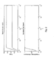
- Fig. 2 shows a smooth and sufficiently detailed resolution at the low end of the timescale. As no mass is lost due to the geometry, the total mass is conserved.
- results are identical to results derived with the complete analytical formulation up to 16 digits.
- the reemission constants must also be considered to be time-dependent. This leads to a time dependency of the matrix A ij of eq. (1) which will be linearized according to eq. (18) with t in t A ⁇ t ⁇ t B .
- F ji - ⁇ ij ⁇ r , j t F ji - ⁇ ij ⁇ r , j t A + t - t A t B - t A F ji - ⁇ ij ⁇ r , j t B - F ji - ⁇ ij ⁇ r , j t A ⁇ A ij + t - t A ⁇ B ij
- Eq.(22) is an inhomogeneous ODE (Ordinary Differential Equation)-system with time dependent coefficients.
- ODE Organic Differential Equation
- the integration has to be carried out for every index pair (j, n).
- the result has first to be multiplied by ⁇ e , n 1 / ⁇ c , n • ⁇ e ⁇ j ⁇ t and then multiplied with the corresponding entry of the matrix P jm - 1 ⁇ F mn T .
- Evaluation of the integral amounts to calculating an incomplete hypergeometric function and can be time consuming.
- matrix A is generally nonsymmetrical and very large, its diagonalisation may become difficult.
- a large matrix whose entries vary over some orders of magnitude may have eigenvectors that are very similar.
- MATLAB® provides the function rank to compute the number of linearly independent rows or columns of a matrix.
- N being the dimension of P and s ii the diagonal matrix consisting of P's singular values.
- the following graph shows the magnitude of the relative error of the sum over all deposits at the end of the simulation time as a function of the number of singular values that were used in the construction of the pseudo inverse.
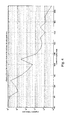
- Fig. 3 shows a graph of the error of total deposit as a function of the number of singular values
- Fig. 4 shows a graph of an error of total deposit as a function of the number of singular values for subsequent runs
- a matrix of dimension n is diagonalizable if and only if it has n linearly independent eigenvectors.
- a matrix is diagonalizable if and only if all its eigenvalues are semi-simple.
- MATLAB® defines ⁇ ( X ) for any double precision number X as the next larger in magnitude floating point number with the same precision as X.
- the structure of the solution requires the knowledge of matrix P lm - 1 .
- Using the inbuild inversion routines of MATLAB® might produce residuals which are considered too large, in particular as the problem matrix A is not symmetric and thus numerical strategies for inversion might not converge fast or accurate enough.
- a left eigenvector of the problem matrix A is the transpose of a right eigenvector of the transposed problem matrix and that a matrix whose rows consist of left eigenvectors is the inverse of the matrix whose columns consist of right eigenvectors.
- P ⁇ new - 1 P ⁇ - 1 - d ⁇ P - 1 and the process is repeated until a given criterion is reached.
- a possible criterion could be 1 - norm ⁇ P * P ⁇ n - th iteration - 1 ⁇ 10 - 12
- the present invention enables the computation of self-contamination at a specific time directly in a single computation step without requiring iterative, time consuming and useless intermediate steps. Moreover, the computed solution is exact within the scope of computation accuracy.
- the method can be implemented as part of a software tool suite for spacecraft computations and simulations.
Landscapes
- Engineering & Computer Science (AREA)
- Physics & Mathematics (AREA)
- Theoretical Computer Science (AREA)
- Aviation & Aerospace Engineering (AREA)
- Remote Sensing (AREA)
- General Physics & Mathematics (AREA)
- Data Mining & Analysis (AREA)
- Mathematical Physics (AREA)
- General Engineering & Computer Science (AREA)
- Critical Care (AREA)
- Health & Medical Sciences (AREA)
- General Health & Medical Sciences (AREA)
- Emergency Medicine (AREA)
- Mathematical Optimization (AREA)
- Databases & Information Systems (AREA)
- Mathematical Analysis (AREA)
- Pure & Applied Mathematics (AREA)
- Software Systems (AREA)
- Computational Mathematics (AREA)
- Algebra (AREA)
- Computer Hardware Design (AREA)
- Evolutionary Computation (AREA)
- Geometry (AREA)
- Complex Calculations (AREA)
- Management, Administration, Business Operations System, And Electronic Commerce (AREA)
Abstract
Description
- The invention relates to a method for computing self-contamination processes of a spacecraft.
- Self-contamination processes of a spacecraft such as a satellite may be caused by molecules, which outgas from surfaces of the spacecraft in vacuum, particularly from coatings, and are desorbed from the surfaces. Self-contamination may cause adverse changes of the characteristics of the surfaces, for example may degrade the spectral and directional characteristics of optical surfaces or the emissivity, absorptivity, and reflectivity of non-optical surfaces. The publication "Spacecraft outgassing, a largely underestimated phenomen", M- Hässig et al., 2nd International Conference on Space Technology (ICST), 15-17 Sept. 2011, pages 1-4 Print ISBN: 978-1-4577-1874-8, discusses the problems caused by outgassing and contamination phenomena measured during the Rosetta spacecraft mission.
- Since such adverse changes may be critical for space missions, analytical models based on numerical methods have been developed for computing self-contamination processes and determining adverse changes before the launch of a critical space mission. Due to the different materials used in modern spacecraft, self-contamination processes occur in highly different time scales. However, the numerical methods used in the known analytical models for computing self-contamination processes require very long computing times particularly at short time scales and usually produce numerical errors.
- The European Space Agency (ESA) provides a software called COMOVA (Contamination Modelling Outgassing & Vent Analyses tool) for spacecraft molecular external contamination modelling (Internet: http://www-mip.onera.fr/comova/). COMOVA allows the computation of contamination of spacecraft surfaces, but requires relatively long computing times. COMOVA may be also used within ESABASE2 Space Engineering Analysis Tool (Internet: http://esabase2.net/product/esabase2-comova/) in order to provide computation of contamination deposits on surfaces, including the calculation of view factors and surface temperature effects.
- It is an object of the present invention to propose a method for computing self-contamination processes of a spacecraft, which can compute results within a time period, which is significantly shorter than the computing time required by computing methods based on known numerical solution schemes, and which produces much more accurate results.
- This object is achieved by the subject matter of the independent claims. Further embodiments are shown by the dependent claims.
- The present invention proposes a novel algorithm for computing self-contamination processes of a spacecraft based on an analytical solution of the mathematical equations underlying the problem of outgassing and self-contamination of different materials of a spacecraft.
- An embodiment of the invention relates to a Method for computing self-contamination processes of a spacecraft by means of a data processing device comprising the following steps: receiving a first set of input parameters comprising general definitions of the spacecraft, receiving a second set of input parameters comprising control parameters for the spacecraft orbital data, physics, numeric, computing a self-contamination process of the spacecraft based on the received first and second sets of input data by calculating an analytical solution of a basic equation for calculating a deposit of molecules outgassed from surfaces of the spacecraft in a single computation step with the data processing device, and outputting the calculated deposit. Depending on the surfaces properties such as piecewise constant or time dependent emission and reemission coefficients, a suitable basic equation for calculating a deposit of molecules outgassed from surfaces of the spacecraft may be selected, which may then be analytically solved in a single computation step, which means that no iterative, time consuming and unneeded intermediate steps are required for computing the solution of the basic equation.
- The step of computing a self-contamination process may comprise the step of computing view factors Fji of a mesh element j of a surface of the spacecraft with respect to a mesh element i of a surface of the spacecraft, wherein the spacecraft is represented as a collection of surfaces, which are subdivided into mesh elements (in the sequel called "nodes") with outgassing properties that can vary from mesh element to mesh element or node to node, respectively.
- The calculating of an analytical solution of the basic equation may comprise calculating the deposit for piecewise constant emission and reemission constants of the surfaces of the spacecraft, with the abbreviated basic equation being


- The calculating of an analytical solution of the basic equation may also comprise calculating the deposit for time dependent emission and reemission coefficients of the surfaces of the spacecraft with a linearized basic equation of the form

interval 0 ≤ t ≤ tA in which matrices A, B are constant:
- A further embodiment of the invention relates to a computer program, which implements the method for computing self-contamination processes of a spacecraft according to the invention and as described herein and enables the computing of self-contamination processes of a spacecraft according to the invention when executed by a computer. Such a computer program could be integrated in a software suite for computing and simulating spacecraft.
- According to a further embodiment of the invention, a record carrier storing a computer program according to the invention may be provided, for example a CD-ROM, a DVD, a memory card, a diskette, or a similar data carrier suitable to store the computer program for electronic access.
- These and other aspects of the invention will be apparent from and elucidated with reference to the embodiments described hereinafter.
- The invention will be described in more detail hereinafter with reference to exemplary embodiments. However, the invention is not limited to these exemplary embodiments.
-
-
Fig. 1 shows schematically the process of self-contamination by means of two surfaces i and j; -
Fig. 2 shows two graphs with a deposit at anode 1 and anode 2 and a normalized total deposit as computed with the method according to the invention for a test case with two plates with constant emission and reemission constants; -
Fig. 3 shows a graph of an error of total deposit as a function of the number of singular values; and -
Fig. 4 shows a graph of an error of total deposit as a function of the number of singular values for subsequent runs. - In the following, functionally similar or identical elements may have the same reference numerals. Absolute values are shown below by way of example only and should not be construed as limiting the invention.
- For computing self-contamination processes of a spacecraft, which particularly comprises different materials, the spacecraft is represented as a collection of surfaces, which are sub-divided into nodes (mesh elements) that have varying outgassing properties and emit and exchange contaminant mass. The contaminant molecules emitted by the surfaces and the bulk of the spacecraft move towards all spacecraft surfaces.
- For computing a self-contamination process of a spacecraft with a data processing device such as a computer, which executes a computer program implementing basic steps of the inventive method, the data processing device receives two sets of input parameters: a first set of input parameters contains general definitions of the spacecraft such as parameters of the geometry of the spacecraft, properties of surfaces of the spacecraft, particularly outgassing/emission and reemission properties of the surfaces or coatings of the surfaces, and temperatures. A second set of input parameters contains control parameters for the spacecraft orbital data, physics, numeric. The spacecraft orbital data typically comprise orbit definition and interpolation data and kinematics data. The control parameters for physics comprise data for atmosphere definition and transport definition. The control parameters for numeric may comprise parameters for raytracing and view factors, parameters regarding surfaces sensitive to contamination and to outgassing, and/or volume mesh data.
- The data processing device processes the received input data for computing a self-contamination process of the spacecraft. The computation comprises calculating an analytical solution of a basic equation for calculating a deposit of molecules outgassed from surfaces of the spacecraft. The computation may be divided in two basic steps:
- 1. Computation of view factors, i.e. the proportion of the total mass emitted by a node i and reaching node j.
- 2. Solution of the integral equation of the deposit as the analytical solution of a basic equation.
- The view factors Fij between two surfaces mesh elements (nodes) i and j are calculated in a first step. The view factors can be defined at macroscopic level as the mass or the molecules emitted by node or surface mesh element i, which reach(es) node or surface mesh element j, divided by the entire mass or all molecules emitted by node or surface mesh element i. At a microscopic level, view factors Fij can be defined as the probability for a molecule emitted by node i reaching node j.
- As shown in
Fig. 1 , the transfer of mass between two nodes i and j comprises direct flux, flux scattered by other contaminant molecules (self-scattering), flux scattered by ambient gas flux (ambient gas scattering), and flux reemitted from spacecraft surfaces. - The view factors Fij can be determined by a Monte-Carlo ray-tracing as briefly explained in the following: a node i randomly emits a large number of rays, which represent the outgassed molecules. The emission of rays can be performed as follows: emission points are sampled according to an iso-distribution law; emission directions are sampled according to Lambert's law. The mean free path λa is based on Robertson formula where the cross-section is computed by the Hard Sphere model. For each ray, a collision distance dc is sampled at random according to the collision probability law P(x) = e -x/ λ
a , where x is the distance and λa is the mean free path. By comparing the distance, the molecule is either scattered or impinges the node j. If dc < dj, a collision is accepted, otherwise it is rejected. If a collision is rejected, the molecule reaches node j and contributes to Fij. If a collision is accepted, the molecule is reemitted from the collision point with a random direction and reaches the node k and contributes to Fik. - After calculating the view factors Fij, the mass deposit can be calculated as briefly outlined in the following: the nodes i, j, k, ... form a network where each pair of elements i, j or i, k or j, k is related by their view factors Fij, Fik or Fjk. Each element has emission, deposition and reemission of deposited contaminants. Thus, this problem becomes a system of differential equations of first order, which can be solved by the inventive solution as explained in the following in detail.
- The computation steps according to the inventive solution and as described in the following can be implemented in a computer program such as an additional module or plug-in for the above mentioned COMOVA-software and can significantly reduce the computation time required for computing self-contamination processes of spacecraft consisting of different materials with different outgassing and desorbing behavior. An annex at the end of the description of embodiments serves to explain some backgrounds of the computation steps and the solving of several equations.
- The equation (as defined in the OUTGASSING Software User's Manual, internal document identification MOS.UM.93694.ASTR, on page 136, equation (72), incorporated herein by reference; simplified form of the equation can be found in Van Eesbeek M., Zwaal A., "Outgassing and Contamination Model Based on Residence Time", Proceedings of the Third European Symposium on Spacecraft Materials in Space Environment, Noordwijk, Oct. 1985, (ESA SP-232)) for the deposit on a node "i" that is to be solved is as follows:

- For the sake of readability, equation (1) is abbreviated to


- It is assumed that t is running in an interval tA ≤ t ≤ tB in which matrix A is constant.
- Then it holds that


- The integration constant c is determined by inserting the boundary condition y(tA ) = yA as deposit at time tA to be

- So that the complete solution takes on the form:

- If matrix A is piecewise constant in successive time intervals the above analysis can be carried out successively in each interval:
-
Let 0 ≤ t 1 ≤ t 2 and - For t1 < t ≤ t 2 the deposit is calculated now as


- Generalizing this to n intervals yields the deposit at time tn of the n-th interval:

- Here y n-1 is the cumulative deposit that had been calculated during the previous n-1 time steps.
- In order to carry out the integration of eq. (8) the eigenvalue decomposition of eq. (2) must be used:


- Eq. (10) describes the time dependency of the deposit in the first time interval between t=0 und t. Here


interval 0 ≤ t ≤ (tn - t n-1) where


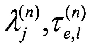
- Eq. (10) seems to contain a singularity as the expression λjτe,l + 1 may become 0 for a certain combination of parameters. It shall show now that this singularity is removable:
-

- If now


- Eq. (1) was solved for two plates with perfect visibility. It was tested whether the computer program MATLAB® from MathWorks Inc. was able to solve the equation using the analytical solution for a time range that extended over 20 orders of magnitude. Results should be calculated at equally spaced points on a log10 scale of the time axis so that a prospective user could check at one glance if peaks occurred even at very low times and what the end-of-life value would be.
- The parameters used were:


-
Fig. 2 shows a smooth and sufficiently detailed resolution at the low end of the timescale. As no mass is lost due to the geometry, the total mass is conserved. - The results are identical to results derived with the complete analytical formulation up to 16 digits.
- In case the emission constant does not depend on time, the emission of material from the bulk is described by

- This equation is the solution of the first order reaction kinetic equation


- In the sequel it shall be assumed that tA ≤ t ≤ tB and that temperature T varies linearly in this interval. The emission laws provided by ESTEC (European Space Research and Technology Centre) and CNES (Centre national d'études spatiales) as well as the Arrhenius law are exponentials in T. Nevertheless it shall be approximated eq. (17) by a finite difference in the interval tA ≤ t ≤ tB :

- This approximation can be applied to the ESTEC and CNES model alike as the finite difference quotient is computed simply by setting the temperatures that prevail at time tA and tB into the emission law that one wishes to use.
- Eq. (18) can be set into eq.(16) and the integration carried out to yield

- Expanding into first order of the slope τ e gives the expression:

- In addition to the emission constants the reemission constants must also be considered to be time-dependent. This leads to a time dependency of the matrix Aij of eq. (1) which will be linearized according to eq. (18) with t in tA ≤ t ≤ tB.

- Again the formulation is independent of the model used (CNES or ESTEC) as only the reemission constants that belong to the temperatures at times tA , tB enter the equation. With the results of the previous chapter the equation for the deposit can be formulated as follows:

- Eq.(22) is an inhomogeneous ODE (Ordinary Differential Equation)-system with time dependent coefficients. In order to apply the method of variation of coefficients like in the chapter "Calculation of deposits for Piecewise constant emission-and reemission constants" a full set of solution vectors called fundamental system of the homogeneous system is needed. Usually it is not possible to calculate the fundamental system analytically. Instead the ODE-system shall be cast into the form of an integral equation which then will be solved approximately using the trapezium rule.
- Using the notation of eq. (2) the eq. (22) now has the form

- Now it holds that

- It is assumed that t is running in an
interval 0 ≤ t ≤ tA in which matrices A, B are constant. - It follows that

- The integration constant c is determined by inserting the boundary condition y(0) = y 0 as deposit at time t=0 to be

- Eq. (28) is rewritten as


- It shall now be approximated using the trapezium rule

- Now

- Solving for y yields

- This inverse matrix is usually not computed explicitly. Instead the system of equations of eq. (30) is solved by Gaussian elimination which is much faster and more accurate.
- The calculation of

- As the emission law does not contain an exp-function any more, the integration cannot be carried out analytically. Instead one has:

- The integration has to be carried out for every index pair (j, n). The result has first to be multiplied by


- Eq. (31) and (32) were solved for the following set of parameters:


- The following table displays the results for various values of t. Deposits calculated from eqs. (31, 32) had been checked with MATLAB®s ODE45 and ODE15s solvers.
t/sec New solver ODE45 ODE15s Max rel. error/% 1e-4 (2.753072, 6.762733)e-2 (2.743272, 6.772533)e-2 (2.742827, 6.772767)e-2 0.35 5e-4 (1.839330, 2.094604)e-1 (1.814627, 2.119308)e-1 (1.814760, 2.119443)e-1 1.3 1e-3 (3.111302, 3.208064)e-1 (3.071725, 3.247641)e-1 (3.073184, 3.249085)e-1 1.3 5e-3 (4.965819, 4.965956)e-1 (4.963851, 4.967924)e-1 (4.959398, 4.961918)e-1 0.04 - As matrix A is generally nonsymmetrical and very large, its diagonalisation may become difficult. A large matrix whose entries vary over some orders of magnitude may have eigenvectors that are very similar.
- Although it is highly unlikely that in practical cases a matrix ever becomes strictly defective in the mathematical sense (see Annex) it may be difficult to decide if eigenvectors are too close to be considered different. If this is the case, matrix P is not invertible because its condition number becomes large and the result will be unreliable because round off errors will be magnified arbitrarily. MATLAB® provides the function rank to compute the number of linearly independent rows or columns of a matrix.
- Rank is defined as the number of all singular values of P which are larger than tol with

- With N being the dimension of P and sii the diagonal matrix consisting of P's singular values.
- Now if rank(P) < N, a complex matrix P cannot be inverted but the inverse can be approximated by the pseudo inverse P+.
- Given the SVD of P as


- In order to quantify the error that is made if the pseudo inverse according to eq.(35) is used instead of the true inverse of P, an analysis was carried out using a non-defective problem matrix Aij of rank N=2161 taken from an ongoing analysis. As the matrix was diagonalizable, a reference value against which the results derived with different pseudo inverses could be tested was available. The deposits were calculated on all nodes in 21 different runs, each time using 100 singular values more than before in building the pseudo inverse. In the 22nd run, which was used as reference, all singular values were used. This reference run was compared to the result derived using the correct inv(P) and produced a relative error smaller than 1e-10.
- The following graph shows the magnitude of the relative error of the sum over all deposits at the end of the simulation time as a function of the number of singular values that were used in the construction of the pseudo inverse.
-
Fig. 3 shows a graph of the error of total deposit as a function of the number of singular values - So using 2100 singular values out of 2161 produces a relative error lower than 1 e-9.
- In case the problem matrix is actually defective a convergence analysis has to be carried out in which results derived using more singular values are compared to results coming from less singular values. A suitable pseudo inverse can be found if the relative error calculated between subsequent runs becomes lower than a defined threshold. The following graph shows how the relative error of the total deposit develops when it is calculated between subsequent runs that use pseudo inverses which differ by 100 singular values. So the rightmost value ( x-axis = 2100) indicates a relative error of lower than 2e-5 when the total deposit calculated with 2100 singular values is compared to the one calculated using 2000 values.
-
Fig. 4 shows a graph of an error of total deposit as a function of the number of singular values for subsequent runs - According to Yousef Saad, "Numerical methods for large eigenvalue problems", Cambridge University Press, 2 nd ed.:
- 1. An eigenvalue λ of A is said to have algebraic multiplicity µ if it is a root of multiplicity µ of the characteristic polynomial.
- 2. If an eigenvalue is of algebraic multiplicity one it is said to be simple. A nonsimple eigenvalue is said to be multiple.
- 3. An eigenvalue λ of A has geometric multiplicity γ if the maximum number of independent eigenvectors associated with it is γ
- 4. A matrix is said to be derogatory if the geometric multiplicity of at least one of its eigenvalues is larger than one.
- 5. An eigenvalue is said to be semi-simple if its algebraic multiplicity is equal to its geometric multiplicity. An eigenvalue that is not semi-simple is called defective.
- The following two statements are equivalent:
- A matrix of dimension n is diagonalizable if and only if it has n linearly independent eigenvectors.
- A matrix is diagonalizable if and only if all its eigenvalues are semi-simple.
- Three cases thus can be distinguished:
- 1. All eigenvalues are distinct: In this case the matrix is diagonalizable.
- 2. All eigenvalues are semi-simple which means that algebraic multiplicity µ>1 but each multiple eigenvalue has µ linearly independent eigenvectors: In this case the matrix is diagonalizable.
- 3. At least one eigenvalue is not semi simple: In this case the matrix is not diagonalizable and is called defective.
- According to IEEE standards the relative machine precision is defined as follows: To a given double precision number x the next distinct double precision number x + ε must obey

- MATLAB® defines ε(X) for any double precision number X as the next larger in magnitude floating point number with the same precision as X.
- The structure of the solution requires the knowledge of matrix

- We can exploit the fact that a left eigenvector of the problem matrix A is the transpose of a right eigenvector of the transposed problem matrix and that a matrix whose rows consist of left eigenvectors is the inverse of the matrix whose columns consist of right eigenvectors.
- If [Vr,Dr]=eig(A) produces the right eigenvectors of A then [VI,DI]=eig(A') produces right eigenvectors of the transposed matrix and thus the transposed left eigenvectors of the problem matrix. It also holds that Dr=DI..It must be assured that MATLAB® orders left and right vectors in an identical order. One can test for diagonality now by computing Vr*VI' = diagonal. Additional scaling of the eigenvectors might be necessary to achieve a unit-diagonal matrix.
- Assuming that as P̃ -1 computed by MATLAB® differs from the correct P -1 according to


- Then it is set


- The present invention enables the computation of self-contamination at a specific time directly in a single computation step without requiring iterative, time consuming and useless intermediate steps. Moreover, the computed solution is exact within the scope of computation accuracy. The method can be implemented as part of a software tool suite for spacecraft computations and simulations.
-
- CNES
- Centre national d'études spatiales
- COMOVA
- COntamination Modelling Outgassing & Vent Analyses tool
- ESTEC
- European Space Research and Technology Centre
- ODE
- Ordinary Differential Equation


Claims (8)
- Method for computing self-contamination processes of a spacecraft by means of a data processing device comprising the following steps:- receiving a first set of input parameters comprising general definitions of the spacecraft,- receiving a second set of input parameters comprising control parameters for the spacecraft orbital data, physics, numeric,- computing a self-contamination process of the spacecraft based on the received first and second sets of input data by calculating an analytical solution of a basic equation for calculating a deposit of molecules outgassed from surfaces of the spacecraft in a single computation step with the data processing device, and- outputting the calculated deposit.
- The method of claim 1, wherein the step of computing a self-contamination process comprises the step of computing view factors Fji of a mesh element j of a surface of the spacecraft with respect to a mesh element i of a surface of the spacecraft, wherein the spacecraft is represented as a collection of surfaces, which are subdivided into mesh elements with outgassing properties, which can vary from mesh element to mesh element.
- The method of claim 2, wherein the calculating of an analytical solution of the basic equation comprises calculating the deposit for piecewise constant emission and reemission constants of the surfaces of the spacecraft, with the abbreviated basic equation being

- The method of claim 3, wherein the calculating the deposit comprises computing the integral equation of the deposit according to the following equation for calculating the deposit at time tn of the n-th time interval:

wherein y n-1 is the cumulative deposit that had been calculated
during the previous n-1 time steps, An is a piecewise constant matrix calculated from the view factors Fji and the reemission coefficients and b(s) is a vector consisting of the emission coefficients, view factors and the initial deposit at time s. - The method of claim 2, wherein the calculating of an analytical solution of the basic equation comprises calculating the deposit for time dependent emission and reemission constants of the surfaces of the spacecraft with a linearized basic equation of the form

with y being the deposit at time t, A and B being constant matrices calculated from the time-dependent view factors Fji and the reemission coefficients and b being a vector consisting of the time-dependent emission coefficients, view factors and the initial deposit. - The method of claim 5, wherein the calculating the deposit comprises computing the integral equation for calculating the deposit at time t, which is running in an interval 0 ≤ t ≤ tA in which matrices A, B are constant:

wherein the integration constant c is determined by inserting the boundary condition y(0) = y 0 as deposit at time t=0 to be C = y 0, and b(s) is a vector consisting of the time-dependent emission coefficients, view factors and the initial deposit at time s. - A computer program implementing a method of any of the preceding claims.
- A record carrier storing a computer program according to claim 7.
Priority Applications (3)
| Application Number | Priority Date | Filing Date | Title |
|---|---|---|---|
| EP13005781.3A EP2883798B1 (en) | 2013-12-12 | 2013-12-12 | Method for computing self-contamination processes of a spacecraft |
| US14/567,204 US10628536B2 (en) | 2013-12-12 | 2014-12-11 | Method for computing self-contamination processes of a spacecraft |
| JP2014250476A JP6410585B2 (en) | 2013-12-12 | 2014-12-11 | Calculation method for the progress of self-contamination of spacecraft |
Applications Claiming Priority (1)
| Application Number | Priority Date | Filing Date | Title |
|---|---|---|---|
| EP13005781.3A EP2883798B1 (en) | 2013-12-12 | 2013-12-12 | Method for computing self-contamination processes of a spacecraft |
Publications (2)
| Publication Number | Publication Date |
|---|---|
| EP2883798A1 true EP2883798A1 (en) | 2015-06-17 |
| EP2883798B1 EP2883798B1 (en) | 2017-06-28 |
Family
ID=49882753
Family Applications (1)
| Application Number | Title | Priority Date | Filing Date |
|---|---|---|---|
| EP13005781.3A Active EP2883798B1 (en) | 2013-12-12 | 2013-12-12 | Method for computing self-contamination processes of a spacecraft |
Country Status (3)
| Country | Link |
|---|---|
| US (1) | US10628536B2 (en) |
| EP (1) | EP2883798B1 (en) |
| JP (1) | JP6410585B2 (en) |
Cited By (2)
| Publication number | Priority date | Publication date | Assignee | Title |
|---|---|---|---|---|
| CN110900621A (en) * | 2019-11-19 | 2020-03-24 | 北京空间技术研制试验中心 | Service method for replacing exposed load of manned spacecraft on orbit based on mechanical arm |
| CN112580201A (en) * | 2020-12-11 | 2021-03-30 | 东风汽车集团有限公司 | Simulation test evaluation method and evaluation system for vehicle emergency steering auxiliary system |
Families Citing this family (2)
| Publication number | Priority date | Publication date | Assignee | Title |
|---|---|---|---|---|
| CN109110159B (en) * | 2018-08-10 | 2020-08-07 | 北京空间技术研制试验中心 | Method for designing spacecraft region revisit orbit |
| CN110733667B (en) * | 2019-09-29 | 2021-06-18 | 北京空间技术研制试验中心 | Design method for inter-orbit transfer of earth-moon translation point |
Family Cites Families (10)
| Publication number | Priority date | Publication date | Assignee | Title |
|---|---|---|---|---|
| JPH11326521A (en) * | 1998-05-15 | 1999-11-26 | Toshiba Corp | Dose etc. prediction monitoring method and its device |
| US6290180B1 (en) * | 1999-09-09 | 2001-09-18 | Lockheed Martin Corporation | Photocatalytic coatings on optical solar reflectors to decompose organic contaminants |
| JP2002228753A (en) * | 2001-01-30 | 2002-08-14 | Nec Aerospace Syst Ltd | Radioactive material diffusion prediction system |
| JP2003106981A (en) * | 2001-09-27 | 2003-04-09 | Nippon Winton Kk | Pollution degree investigation system, pollution degree investigation method and detector |
| JP2006133121A (en) * | 2004-11-08 | 2006-05-25 | Daikin Ind Ltd | Base, air pollution information providing system, air pollution prediction method, and ventilation device |
| JP2008151694A (en) * | 2006-12-19 | 2008-07-03 | Nippon Telegr & Teleph Corp <Ntt> | Contaminated environment predicting device in depression, method for predicting contaminated environment in depression, and program for executing the prediction method |
| FR2922667A1 (en) * | 2007-10-22 | 2009-04-24 | Commissariat Energie Atomique | METHOD FOR MANAGING A TIME-EVOLVING ACCIDENT |
| JP2009162502A (en) * | 2007-12-28 | 2009-07-23 | Mitsubishi Heavy Ind Ltd | Computing system of exposure amount |
| FR2957416B1 (en) * | 2010-03-12 | 2012-04-20 | Thales Sa | DEVICE FOR QUANTIFYING THE DEGASSING OF EQUIPMENT PLACED IN A VACUUM ENCLOSURE |
| JP5738140B2 (en) * | 2011-09-16 | 2015-06-17 | 三菱重工業株式会社 | Substance release amount estimation apparatus, method and program |
-
2013
- 2013-12-12 EP EP13005781.3A patent/EP2883798B1/en active Active
-
2014
- 2014-12-11 US US14/567,204 patent/US10628536B2/en active Active
- 2014-12-11 JP JP2014250476A patent/JP6410585B2/en active Active
Non-Patent Citations (6)
| Title |
|---|
| B. SCHLÄPPI ET AL: "Influence of spacecraft outgassing on the exploration of tenuous atmospheres with in situ mass spectrometry", JOURNAL OF GEOPHYSICAL RESEARCH: SPACE PHYSICS. VOL. 115, ISS. A12, 14 December 2010 (2010-12-14), XP055120981, Retrieved from the Internet <URL:http://onlinelibrary.wiley.com/enhanced/doi/10.1029/2010JA015734/> [retrieved on 20140602] * |
| DR. KARL DIETRICH BUNTE ET AL: "ESABASE2 GUI | ESABASE2 - Graphical User Interface", 14 November 2011 (2011-11-14), XP055120959, Retrieved from the Internet <URL:http://web.archive.org/web/20111114025559/http://esabase2.net/screenshots/esabase2-gui/> [retrieved on 20140602] * |
| ESA AND ONERA: "COMOVA General Organisation - Input Parameters", 31 December 2001 (2001-12-31), XP055120954, Retrieved from the Internet <URL:http://www-mip.onera.fr/comova/html/comova/organisation/mn_orga.htm?nTrio=7> [retrieved on 20140602] * |
| ESA AND ONERA: "COMOVA The Physics - Contaminant Transport", 31 December 2001 (2001-12-31), XP055120961, Retrieved from the Internet <URL:http://www-mip.onera.fr/comova/html/comova/param/mn_param.htm?nTrio=8> [retrieved on 20140602] * |
| J-F ROUSSEL ET AL: "A NEW FRONTIER FOR CONTAMINATION: REACHING THE MOLECULES", 5 October 2009 (2009-10-05), XP055120983, Retrieved from the Internet <URL:http://esmat.esa.int/materials_news/isme09/pdf/1-Opening/Roussel.pdf> [retrieved on 20140602] * |
| R RAMPINI ET AL: "DYNAMIC OUTGASSING TESTING: A REVISITED MATHEMATICAL APPROACH", 16 August 2009 (2009-08-16), XP055120982, Retrieved from the Internet <URL:http://esmat.esa.int/materials_news/isme09/pdf/6-Contamination/Poster Contamination - Rampini.pdf> [retrieved on 20140602] * |
Cited By (4)
| Publication number | Priority date | Publication date | Assignee | Title |
|---|---|---|---|---|
| CN110900621A (en) * | 2019-11-19 | 2020-03-24 | 北京空间技术研制试验中心 | Service method for replacing exposed load of manned spacecraft on orbit based on mechanical arm |
| CN110900621B (en) * | 2019-11-19 | 2021-05-18 | 北京空间技术研制试验中心 | Service method for replacing exposed load of manned spacecraft on orbit based on mechanical arm |
| CN112580201A (en) * | 2020-12-11 | 2021-03-30 | 东风汽车集团有限公司 | Simulation test evaluation method and evaluation system for vehicle emergency steering auxiliary system |
| CN112580201B (en) * | 2020-12-11 | 2022-11-08 | 东风汽车集团有限公司 | Simulation test evaluation method and system for vehicle emergency steering auxiliary system |
Also Published As
| Publication number | Publication date |
|---|---|
| JP6410585B2 (en) | 2018-10-24 |
| JP2015113121A (en) | 2015-06-22 |
| US20150169805A1 (en) | 2015-06-18 |
| US10628536B2 (en) | 2020-04-21 |
| EP2883798B1 (en) | 2017-06-28 |
Similar Documents
| Publication | Publication Date | Title |
|---|---|---|
| van Haasteren et al. | New advances in the Gaussian-process approach to pulsar-timing data analysis | |
| CN110795887B (en) | Multi-stress accelerated life test analysis method and device | |
| Frezat et al. | Physical invariance in neural networks for subgrid-scale scalar flux modeling | |
| Ito et al. | The complex Langevin analysis of spontaneous symmetry breaking induced by complex fermion determinant | |
| Nino-Ruiz et al. | An ensemble Kalman filter implementation based on modified Cholesky decomposition for inverse covariance matrix estimation | |
| Langfeld et al. | Density of states approach to dense quantum systems | |
| EP2883798B1 (en) | Method for computing self-contamination processes of a spacecraft | |
| Poterjoy et al. | Systematic comparison of four-dimensional data assimilation methods with and without the tangent linear model using hybrid background error covariance: E4DVar versus 4DEnVar | |
| Patton et al. | Application of preconditioned GMRES to the numerical solution of the neutron transport equation | |
| Lewis et al. | Gradient free active subspace construction using Morris screening elementary effects | |
| Blanes et al. | Applying splitting methods with complex coefficients to the numerical integration of unitary problems | |
| Whittaker et al. | A comparison of empirical and experimental O7+, O8+, and O/H values, with applications to terrestrial solar wind charge exchange | |
| Seko et al. | Projector-based efficient estimation of force constants | |
| Giraud et al. | Iterative versus direct parallel substructuring methods in semiconductor device modelling | |
| Losacco et al. | A differential algebra-based importance sampling method for impact probability computation on Earth resonant returns of near-Earth objects | |
| Xu et al. | Efficient algorithms for computing multidimensional integral fractional Laplacians via spherical means | |
| Iwashita et al. | Convergence acceleration of preconditioned conjugate gradient solver based on error vector sampling for a sequence of linear systems | |
| Munier | Statistical physics in QCD evolution towards high energies | |
| Jones et al. | Conjunction assessment using polynomial chaos expansions | |
| Muhiddin et al. | Numerical evaluation of quarter-sweep KSOR method to solve time-fractional parabolic equations | |
| EP3021229A1 (en) | Method for computing self-contamination processes of a spacecraft | |
| Rostkowski et al. | Quantification of uncertainty in extrapolation of charring ablator material performance to flight | |
| Xhako et al. | Fast algorithms for simulating chiral fermions in U (1) lattice gauge theory | |
| Coburger et al. | The bounding problem: Single event effect rate prediction using markov chain monte carlo | |
| Schreiber et al. | Electronic states in the Anderson model of localization: benchmarking eigenvalue algorithms |
Legal Events
| Date | Code | Title | Description |
|---|---|---|---|
| PUAI | Public reference made under article 153(3) epc to a published international application that has entered the european phase |
Free format text: ORIGINAL CODE: 0009012 |
|
| 17P | Request for examination filed |
Effective date: 20131212 |
|
| AK | Designated contracting states |
Kind code of ref document: A1 Designated state(s): AL AT BE BG CH CY CZ DE DK EE ES FI FR GB GR HR HU IE IS IT LI LT LU LV MC MK MT NL NO PL PT RO RS SE SI SK SM TR |
|
| AX | Request for extension of the european patent |
Extension state: BA ME |
|
| R17P | Request for examination filed (corrected) |
Effective date: 20151201 |
|
| REG | Reference to a national code |
Ref country code: DE Ref legal event code: R079 Ref document number: 602013022736 Country of ref document: DE Free format text: PREVIOUS MAIN CLASS: B64G0001220000 Ipc: B64G0099000000 |
|
| RIC1 | Information provided on ipc code assigned before grant |
Ipc: B64G 1/52 20060101ALI20161115BHEP Ipc: B64G 1/22 20060101ALI20161115BHEP Ipc: G06F 17/50 20060101ALI20161115BHEP Ipc: G06F 17/10 20060101ALI20161115BHEP Ipc: B64G 99/00 20090101AFI20161115BHEP |
|
| GRAP | Despatch of communication of intention to grant a patent |
Free format text: ORIGINAL CODE: EPIDOSNIGR1 |
|
| STAA | Information on the status of an ep patent application or granted ep patent |
Free format text: STATUS: GRANT OF PATENT IS INTENDED |
|
| INTG | Intention to grant announced |
Effective date: 20170120 |
|
| GRAS | Grant fee paid |
Free format text: ORIGINAL CODE: EPIDOSNIGR3 |
|
| GRAA | (expected) grant |
Free format text: ORIGINAL CODE: 0009210 |
|
| STAA | Information on the status of an ep patent application or granted ep patent |
Free format text: STATUS: THE PATENT HAS BEEN GRANTED |
|
| AK | Designated contracting states |
Kind code of ref document: B1 Designated state(s): AL AT BE BG CH CY CZ DE DK EE ES FI FR GB GR HR HU IE IS IT LI LT LU LV MC MK MT NL NO PL PT RO RS SE SI SK SM TR |
|
| REG | Reference to a national code |
Ref country code: GB Ref legal event code: FG4D |
|
| REG | Reference to a national code |
Ref country code: CH Ref legal event code: EP |
|
| REG | Reference to a national code |
Ref country code: AT Ref legal event code: REF Ref document number: 904601 Country of ref document: AT Kind code of ref document: T Effective date: 20170715 |
|
| REG | Reference to a national code |
Ref country code: IE Ref legal event code: FG4D |
|
| REG | Reference to a national code |
Ref country code: DE Ref legal event code: R096 Ref document number: 602013022736 Country of ref document: DE |
|
| PG25 | Lapsed in a contracting state [announced via postgrant information from national office to epo] |
Ref country code: NO Free format text: LAPSE BECAUSE OF FAILURE TO SUBMIT A TRANSLATION OF THE DESCRIPTION OR TO PAY THE FEE WITHIN THE PRESCRIBED TIME-LIMIT Effective date: 20170928 Ref country code: FI Free format text: LAPSE BECAUSE OF FAILURE TO SUBMIT A TRANSLATION OF THE DESCRIPTION OR TO PAY THE FEE WITHIN THE PRESCRIBED TIME-LIMIT Effective date: 20170628 Ref country code: LT Free format text: LAPSE BECAUSE OF FAILURE TO SUBMIT A TRANSLATION OF THE DESCRIPTION OR TO PAY THE FEE WITHIN THE PRESCRIBED TIME-LIMIT Effective date: 20170628 Ref country code: HR Free format text: LAPSE BECAUSE OF FAILURE TO SUBMIT A TRANSLATION OF THE DESCRIPTION OR TO PAY THE FEE WITHIN THE PRESCRIBED TIME-LIMIT Effective date: 20170628 Ref country code: GR Free format text: LAPSE BECAUSE OF FAILURE TO SUBMIT A TRANSLATION OF THE DESCRIPTION OR TO PAY THE FEE WITHIN THE PRESCRIBED TIME-LIMIT Effective date: 20170929 |
|
| REG | Reference to a national code |
Ref country code: NL Ref legal event code: MP Effective date: 20170628 |
|
| REG | Reference to a national code |
Ref country code: LT Ref legal event code: MG4D |
|
| REG | Reference to a national code |
Ref country code: AT Ref legal event code: MK05 Ref document number: 904601 Country of ref document: AT Kind code of ref document: T Effective date: 20170628 |
|
| PG25 | Lapsed in a contracting state [announced via postgrant information from national office to epo] |
Ref country code: NL Free format text: LAPSE BECAUSE OF FAILURE TO SUBMIT A TRANSLATION OF THE DESCRIPTION OR TO PAY THE FEE WITHIN THE PRESCRIBED TIME-LIMIT Effective date: 20170628 Ref country code: RS Free format text: LAPSE BECAUSE OF FAILURE TO SUBMIT A TRANSLATION OF THE DESCRIPTION OR TO PAY THE FEE WITHIN THE PRESCRIBED TIME-LIMIT Effective date: 20170628 Ref country code: LV Free format text: LAPSE BECAUSE OF FAILURE TO SUBMIT A TRANSLATION OF THE DESCRIPTION OR TO PAY THE FEE WITHIN THE PRESCRIBED TIME-LIMIT Effective date: 20170628 Ref country code: BG Free format text: LAPSE BECAUSE OF FAILURE TO SUBMIT A TRANSLATION OF THE DESCRIPTION OR TO PAY THE FEE WITHIN THE PRESCRIBED TIME-LIMIT Effective date: 20170928 Ref country code: SE Free format text: LAPSE BECAUSE OF FAILURE TO SUBMIT A TRANSLATION OF THE DESCRIPTION OR TO PAY THE FEE WITHIN THE PRESCRIBED TIME-LIMIT Effective date: 20170628 |
|
| REG | Reference to a national code |
Ref country code: FR Ref legal event code: PLFP Year of fee payment: 5 |
|
| REG | Reference to a national code |
Ref country code: DE Ref legal event code: R082 Ref document number: 602013022736 Country of ref document: DE Representative=s name: WUESTHOFF & WUESTHOFF, PATENTANWAELTE PARTG MB, DE Ref country code: DE Ref legal event code: R081 Ref document number: 602013022736 Country of ref document: DE Owner name: AIRBUS DEFENCE AND SPACE GMBH, DE Free format text: FORMER OWNER: AIRBUS DS GMBH, 82024 TAUFKIRCHEN, DE |
|
| PG25 | Lapsed in a contracting state [announced via postgrant information from national office to epo] |
Ref country code: EE Free format text: LAPSE BECAUSE OF FAILURE TO SUBMIT A TRANSLATION OF THE DESCRIPTION OR TO PAY THE FEE WITHIN THE PRESCRIBED TIME-LIMIT Effective date: 20170628 Ref country code: SK Free format text: LAPSE BECAUSE OF FAILURE TO SUBMIT A TRANSLATION OF THE DESCRIPTION OR TO PAY THE FEE WITHIN THE PRESCRIBED TIME-LIMIT Effective date: 20170628 Ref country code: RO Free format text: LAPSE BECAUSE OF FAILURE TO SUBMIT A TRANSLATION OF THE DESCRIPTION OR TO PAY THE FEE WITHIN THE PRESCRIBED TIME-LIMIT Effective date: 20170628 Ref country code: CZ Free format text: LAPSE BECAUSE OF FAILURE TO SUBMIT A TRANSLATION OF THE DESCRIPTION OR TO PAY THE FEE WITHIN THE PRESCRIBED TIME-LIMIT Effective date: 20170628 Ref country code: AT Free format text: LAPSE BECAUSE OF FAILURE TO SUBMIT A TRANSLATION OF THE DESCRIPTION OR TO PAY THE FEE WITHIN THE PRESCRIBED TIME-LIMIT Effective date: 20170628 |
|
| PG25 | Lapsed in a contracting state [announced via postgrant information from national office to epo] |
Ref country code: ES Free format text: LAPSE BECAUSE OF FAILURE TO SUBMIT A TRANSLATION OF THE DESCRIPTION OR TO PAY THE FEE WITHIN THE PRESCRIBED TIME-LIMIT Effective date: 20170628 Ref country code: IS Free format text: LAPSE BECAUSE OF FAILURE TO SUBMIT A TRANSLATION OF THE DESCRIPTION OR TO PAY THE FEE WITHIN THE PRESCRIBED TIME-LIMIT Effective date: 20171028 Ref country code: SM Free format text: LAPSE BECAUSE OF FAILURE TO SUBMIT A TRANSLATION OF THE DESCRIPTION OR TO PAY THE FEE WITHIN THE PRESCRIBED TIME-LIMIT Effective date: 20170628 Ref country code: PL Free format text: LAPSE BECAUSE OF FAILURE TO SUBMIT A TRANSLATION OF THE DESCRIPTION OR TO PAY THE FEE WITHIN THE PRESCRIBED TIME-LIMIT Effective date: 20170628 |
|
| REG | Reference to a national code |
Ref country code: DE Ref legal event code: R097 Ref document number: 602013022736 Country of ref document: DE |
|
| RAP2 | Party data changed (patent owner data changed or rights of a patent transferred) |
Owner name: AIRBUS DEFENCE AND SPACE GMBH |
|
| PG25 | Lapsed in a contracting state [announced via postgrant information from national office to epo] |
Ref country code: DK Free format text: LAPSE BECAUSE OF FAILURE TO SUBMIT A TRANSLATION OF THE DESCRIPTION OR TO PAY THE FEE WITHIN THE PRESCRIBED TIME-LIMIT Effective date: 20170628 |
|
| PLBE | No opposition filed within time limit |
Free format text: ORIGINAL CODE: 0009261 |
|
| 26N | No opposition filed |
Effective date: 20180329 |
|
| REG | Reference to a national code |
Ref country code: CH Ref legal event code: PL |
|
| GBPC | Gb: european patent ceased through non-payment of renewal fee |
Effective date: 20171212 |
|
| PG25 | Lapsed in a contracting state [announced via postgrant information from national office to epo] |
Ref country code: SI Free format text: LAPSE BECAUSE OF FAILURE TO SUBMIT A TRANSLATION OF THE DESCRIPTION OR TO PAY THE FEE WITHIN THE PRESCRIBED TIME-LIMIT Effective date: 20170628 |
|
| REG | Reference to a national code |
Ref country code: IE Ref legal event code: MM4A |
|
| PG25 | Lapsed in a contracting state [announced via postgrant information from national office to epo] |
Ref country code: MT Free format text: LAPSE BECAUSE OF NON-PAYMENT OF DUE FEES Effective date: 20171212 Ref country code: LU Free format text: LAPSE BECAUSE OF NON-PAYMENT OF DUE FEES Effective date: 20171212 |
|
| REG | Reference to a national code |
Ref country code: BE Ref legal event code: MM Effective date: 20171231 |
|
| PG25 | Lapsed in a contracting state [announced via postgrant information from national office to epo] |
Ref country code: IE Free format text: LAPSE BECAUSE OF NON-PAYMENT OF DUE FEES Effective date: 20171212 |
|
| PG25 | Lapsed in a contracting state [announced via postgrant information from national office to epo] |
Ref country code: CH Free format text: LAPSE BECAUSE OF NON-PAYMENT OF DUE FEES Effective date: 20171231 Ref country code: GB Free format text: LAPSE BECAUSE OF NON-PAYMENT OF DUE FEES Effective date: 20171212 Ref country code: BE Free format text: LAPSE BECAUSE OF NON-PAYMENT OF DUE FEES Effective date: 20171231 Ref country code: LI Free format text: LAPSE BECAUSE OF NON-PAYMENT OF DUE FEES Effective date: 20171231 |
|
| PG25 | Lapsed in a contracting state [announced via postgrant information from national office to epo] |
Ref country code: MC Free format text: LAPSE BECAUSE OF FAILURE TO SUBMIT A TRANSLATION OF THE DESCRIPTION OR TO PAY THE FEE WITHIN THE PRESCRIBED TIME-LIMIT Effective date: 20170628 Ref country code: HU Free format text: LAPSE BECAUSE OF FAILURE TO SUBMIT A TRANSLATION OF THE DESCRIPTION OR TO PAY THE FEE WITHIN THE PRESCRIBED TIME-LIMIT; INVALID AB INITIO Effective date: 20131212 |
|
| PG25 | Lapsed in a contracting state [announced via postgrant information from national office to epo] |
Ref country code: CY Free format text: LAPSE BECAUSE OF FAILURE TO SUBMIT A TRANSLATION OF THE DESCRIPTION OR TO PAY THE FEE WITHIN THE PRESCRIBED TIME-LIMIT Effective date: 20170628 |
|
| PG25 | Lapsed in a contracting state [announced via postgrant information from national office to epo] |
Ref country code: MK Free format text: LAPSE BECAUSE OF FAILURE TO SUBMIT A TRANSLATION OF THE DESCRIPTION OR TO PAY THE FEE WITHIN THE PRESCRIBED TIME-LIMIT Effective date: 20170628 |
|
| PG25 | Lapsed in a contracting state [announced via postgrant information from national office to epo] |
Ref country code: TR Free format text: LAPSE BECAUSE OF FAILURE TO SUBMIT A TRANSLATION OF THE DESCRIPTION OR TO PAY THE FEE WITHIN THE PRESCRIBED TIME-LIMIT Effective date: 20170628 |
|
| PG25 | Lapsed in a contracting state [announced via postgrant information from national office to epo] |
Ref country code: PT Free format text: LAPSE BECAUSE OF FAILURE TO SUBMIT A TRANSLATION OF THE DESCRIPTION OR TO PAY THE FEE WITHIN THE PRESCRIBED TIME-LIMIT Effective date: 20170628 |
|
| PG25 | Lapsed in a contracting state [announced via postgrant information from national office to epo] |
Ref country code: AL Free format text: LAPSE BECAUSE OF FAILURE TO SUBMIT A TRANSLATION OF THE DESCRIPTION OR TO PAY THE FEE WITHIN THE PRESCRIBED TIME-LIMIT Effective date: 20170628 |
|
| STAA | Information on the status of an ep patent application or granted ep patent |
Free format text: STATUS: NO OPPOSITION FILED WITHIN TIME LIMIT |
|
| PGFP | Annual fee paid to national office [announced via postgrant information from national office to epo] |
Ref country code: DE Payment date: 20251211 Year of fee payment: 13 |
|
| PGFP | Annual fee paid to national office [announced via postgrant information from national office to epo] |
Ref country code: IT Payment date: 20251223 Year of fee payment: 13 |
|
| PGFP | Annual fee paid to national office [announced via postgrant information from national office to epo] |
Ref country code: FR Payment date: 20251223 Year of fee payment: 13 |