EP2850500B1 - Predictive temperature management system controller - Google Patents
Predictive temperature management system controller Download PDFInfo
- Publication number
- EP2850500B1 EP2850500B1 EP13706687.4A EP13706687A EP2850500B1 EP 2850500 B1 EP2850500 B1 EP 2850500B1 EP 13706687 A EP13706687 A EP 13706687A EP 2850500 B1 EP2850500 B1 EP 2850500B1
- Authority
- EP
- European Patent Office
- Prior art keywords
- temperature
- energy
- cost
- room
- controller
- Prior art date
- Legal status (The legal status is an assumption and is not a legal conclusion. Google has not performed a legal analysis and makes no representation as to the accuracy of the status listed.)
- Active
Links
Images




Classifications
-
- G—PHYSICS
- G05—CONTROLLING; REGULATING
- G05D—SYSTEMS FOR CONTROLLING OR REGULATING NON-ELECTRIC VARIABLES
- G05D23/00—Control of temperature
- G05D23/19—Control of temperature characterised by the use of electric means
- G05D23/1919—Control of temperature characterised by the use of electric means characterised by the type of controller
- G05D23/1923—Control of temperature characterised by the use of electric means characterised by the type of controller using thermal energy, the cost of which varies in function of time
-
- F—MECHANICAL ENGINEERING; LIGHTING; HEATING; WEAPONS; BLASTING
- F24—HEATING; RANGES; VENTILATING
- F24F—AIR-CONDITIONING; AIR-HUMIDIFICATION; VENTILATION; USE OF AIR CURRENTS FOR SCREENING
- F24F11/00—Control or safety arrangements
- F24F11/30—Control or safety arrangements for purposes related to the operation of the system, e.g. for safety or monitoring
-
- F—MECHANICAL ENGINEERING; LIGHTING; HEATING; WEAPONS; BLASTING
- F24—HEATING; RANGES; VENTILATING
- F24F—AIR-CONDITIONING; AIR-HUMIDIFICATION; VENTILATION; USE OF AIR CURRENTS FOR SCREENING
- F24F11/00—Control or safety arrangements
- F24F11/30—Control or safety arrangements for purposes related to the operation of the system, e.g. for safety or monitoring
- F24F11/46—Improving electric energy efficiency or saving
- F24F11/47—Responding to energy costs
-
- F—MECHANICAL ENGINEERING; LIGHTING; HEATING; WEAPONS; BLASTING
- F24—HEATING; RANGES; VENTILATING
- F24F—AIR-CONDITIONING; AIR-HUMIDIFICATION; VENTILATION; USE OF AIR CURRENTS FOR SCREENING
- F24F11/00—Control or safety arrangements
- F24F11/50—Control or safety arrangements characterised by user interfaces or communication
- F24F11/56—Remote control
- F24F11/58—Remote control using Internet communication
-
- F—MECHANICAL ENGINEERING; LIGHTING; HEATING; WEAPONS; BLASTING
- F24—HEATING; RANGES; VENTILATING
- F24F—AIR-CONDITIONING; AIR-HUMIDIFICATION; VENTILATION; USE OF AIR CURRENTS FOR SCREENING
- F24F11/00—Control or safety arrangements
- F24F11/62—Control or safety arrangements characterised by the type of control or by internal processing, e.g. using fuzzy logic, adaptive control or estimation of values
-
- F—MECHANICAL ENGINEERING; LIGHTING; HEATING; WEAPONS; BLASTING
- F24—HEATING; RANGES; VENTILATING
- F24F—AIR-CONDITIONING; AIR-HUMIDIFICATION; VENTILATION; USE OF AIR CURRENTS FOR SCREENING
- F24F11/00—Control or safety arrangements
- F24F11/62—Control or safety arrangements characterised by the type of control or by internal processing, e.g. using fuzzy logic, adaptive control or estimation of values
- F24F11/63—Electronic processing
-
- G—PHYSICS
- G05—CONTROLLING; REGULATING
- G05B—CONTROL OR REGULATING SYSTEMS IN GENERAL; FUNCTIONAL ELEMENTS OF SUCH SYSTEMS; MONITORING OR TESTING ARRANGEMENTS FOR SUCH SYSTEMS OR ELEMENTS
- G05B15/00—Systems controlled by a computer
- G05B15/02—Systems controlled by a computer electric
-
- G—PHYSICS
- G06—COMPUTING OR CALCULATING; COUNTING
- G06N—COMPUTING ARRANGEMENTS BASED ON SPECIFIC COMPUTATIONAL MODELS
- G06N5/00—Computing arrangements using knowledge-based models
- G06N5/04—Inference or reasoning models
-
- F—MECHANICAL ENGINEERING; LIGHTING; HEATING; WEAPONS; BLASTING
- F24—HEATING; RANGES; VENTILATING
- F24F—AIR-CONDITIONING; AIR-HUMIDIFICATION; VENTILATION; USE OF AIR CURRENTS FOR SCREENING
- F24F11/00—Control or safety arrangements
- F24F11/30—Control or safety arrangements for purposes related to the operation of the system, e.g. for safety or monitoring
- F24F11/46—Improving electric energy efficiency or saving
-
- F—MECHANICAL ENGINEERING; LIGHTING; HEATING; WEAPONS; BLASTING
- F24—HEATING; RANGES; VENTILATING
- F24F—AIR-CONDITIONING; AIR-HUMIDIFICATION; VENTILATION; USE OF AIR CURRENTS FOR SCREENING
- F24F11/00—Control or safety arrangements
- F24F11/62—Control or safety arrangements characterised by the type of control or by internal processing, e.g. using fuzzy logic, adaptive control or estimation of values
- F24F11/63—Electronic processing
- F24F11/64—Electronic processing using pre-stored data
-
- F—MECHANICAL ENGINEERING; LIGHTING; HEATING; WEAPONS; BLASTING
- F24—HEATING; RANGES; VENTILATING
- F24F—AIR-CONDITIONING; AIR-HUMIDIFICATION; VENTILATION; USE OF AIR CURRENTS FOR SCREENING
- F24F2110/00—Control inputs relating to air properties
- F24F2110/10—Temperature
-
- F—MECHANICAL ENGINEERING; LIGHTING; HEATING; WEAPONS; BLASTING
- F24—HEATING; RANGES; VENTILATING
- F24F—AIR-CONDITIONING; AIR-HUMIDIFICATION; VENTILATION; USE OF AIR CURRENTS FOR SCREENING
- F24F2130/00—Control inputs relating to environmental factors not covered by group F24F2110/00
-
- F—MECHANICAL ENGINEERING; LIGHTING; HEATING; WEAPONS; BLASTING
- F24—HEATING; RANGES; VENTILATING
- F24F—AIR-CONDITIONING; AIR-HUMIDIFICATION; VENTILATION; USE OF AIR CURRENTS FOR SCREENING
- F24F2130/00—Control inputs relating to environmental factors not covered by group F24F2110/00
- F24F2130/10—Weather information or forecasts
Definitions
- This invention relates to a controller for a temperature management system, and to a method of controlling such a system.
- the invention is particularly applicable to temperature management systems, such as heating and/or air conditioning systems, that are used to control the temperature of one or more rooms in a building or other structure.
- the invention is more particularly, but not exclusively, concerned with domestic space heating systems and their control.
- Most domestic space heating systems control the temperature by targeting a set point temperature (which may form part of a schedule of set point temperatures that vary over a control period) and using a thermostat with hysteresis to turn the heat source on and off.
- This level of control is based only on the current state of the house and its heating system, and does not take into account any forward planning or knowledge of the thermal response of the house. Consequently, this known method of control can fail to achieve energy efficiency and/or the best comfort for the occupants of the house. For example, the room temperature is prone to fluctuate significantly under thermostatic control and can be uncomfortably low for the first part of a period with a raised set point temperature.
- EP0688085 shows a temperature control system, in which known thermal properties of a building are used to predict temperatures which would be achieved by various possible energy inputs, and this information is used to formulate an energy input schedule that ensures that the building temperature does not fall below temperatures specified in a set point schedule. That schedule can exploit potential cost savings arising from a variable energy tariff, but can lead to room temperatures very much higher than the desired set point temperature, and cannot permit a compromise where the set point schedule would be even slightly violated in order to save energy.
- Huval, B.; Barooah, P "Optimization of a Heating System Using Smart Meters & Dynamic Pricing", University of Florida Undergraduate Honors Thesis, 341 August 2010 , discusses predictive temperature management in which temperatures can deviate from a fixed deal temperature, but cannot accommodate a schedule of set temperatures.
- a controller for a temperature management system for heating and/or cooling a room in accordance with a schedule of set point temperatures over a control period comprising a data processor arrangement; a temperature input for receiving a signal indicative of the current temperature in the room; a control output for supplying control signals to the system; and at least one electronic memory for storing said schedule of set point temperatures, a relationship, based on known heating or cooling characteristics of the room, between the energy supplied to the system in a portion of the control period and the predicted temperature of the room during that portion and subsequent portions of the control period, a first parameter value representative of the cost of supplying said energy and a second parameter value representative of a predetermined acceptability of variations of the actual or predicted temperature of the room from the set point schedule, wherein processor arrangement is operable to calculate, for each said portion, the energy to be supplied to the system in order for a plurality of parameter values to satisfy a predetermined criterion, said plurality of parameter values comprising said first parameter value
- a controller in accordance with the present invention can provide control for a temperature management system which not only takes into account the schedule of set point temperatures, but also a balance between the cost or notional cost of maintaining room temperature in accordance with the schedule and the effect of departures from that schedule. This enables the control of the temperature management system to be optimised so as to achieve the most effective use of energy to maintain the room at a comfortable temperature.
- the controller also takes into account the effect of an energy input in a given portion of the control period on the room temperature in that portion and also in subsequent portions of the period.
- the controller may to advantage be preprogrammed with said relationship between the energy supplied to the systems in a portion of the control period and the predicted temperature of the room during that and subsequent portions of the control period stored in the memory, and is preferably arranged for the user to enter the set point temperature schedule.
- the criterion is applied to the sum of the parameter values.
- the criterion is preferably that the sum of the two values is substantially at a minimum.
- the sum may, for example, be substantially at a minimum at the actual turning point defining the minimum or at an approximate minimum determined by an iterative process such as the gradient descent method or the Newton's method.
- the approximate minimum is determined by the Primal-dual barrier function method.
- the sum is of the values over the whole control period.
- the data processor arrangement is operable to update said calculations for each of the portions over the course of the control period. This enables departures of the current temperatures from those previously predicted to be taken into account.
- the control period may conveniently be of 24 hours' duration, each portion being of 15 minutes' duration so that the period is constituted by 96 consecutive portions.
- the first parameter value comprises the product of the energy to be supplied to the system and an energy cost multiplier.
- This multiplier may vary over the course of the control period to take into account variations in the actual cost of consuming energy, as happens in the case of a smart grid electrical energy supply system, where the cost per unit of energy (usually electrical energy) supplied will vary or in the efficiency of the system, for example in the case of a heat pump, the efficiency of which will vary greatly with the temperature difference between the heat source and the heat sink of the pump.
- the second parameter value comprises the product of a comfort cost multiplier and the difference between the set point temperature and the actual or predicted temperature at the time.
- the second parameter value can thus be considered to be a discomfort cost.
- the second parameter value can be expressed as a discomfort cost, for example to an occupier of the room.
- the criterion, with these two types of parameter value may be that said total is minimised, subject to a fixed energy cost.
- the user could specify the cost of energy to be consumed, and in response, the controller will determine a control schedule which achieves this with minimum discomfort cost.
- the discomfort cost multiplier may vary over the course of a day/control period to account for, for example, levels of occupancy of the room, or the likely activity level of an occupant.
- the multiplier might be lower at night, when the occupant is in bed.
- said relationship is based on a heat transfer model that takes into account at least one of:
- the properties listed at (c) above include the forecasted temperatures of the environment outside the room over the control period.
- the way in which the temperature management system is controlled to have the calculated amount of energy supplied to it may depend on the nature of the temperature management system itself.
- a system comprises a boiler
- the only type of allowable control of the boiler's operation may be switching the boiler (or its burner) on or off.
- the controller may control the boiler by means of a suitable algorithm that simply turns the boiler on for a sufficient proportion of the portion for the calculated amount of energy for that portion to be supplied to, and hence consumed by, the boiler.
- the control system may supply the boiler with a control signal in the form of a series of pulses, each of which defines a period when the boiler is on.
- This signal can be pulse code modulated to provide short term control for the amount of energy delivered.
- modulation may be subject to conditions arising from operational constraints on the boiler, for example a minimum interval between successive activating pulses, to avoid damage or excessive wear to the temperature management system.
- the controller may be operable, during each portion, to use the predicted temperature profile associated with the calculated energy inputs as a target for the boiler and to compare this profile with further predicted temperatures for a part of the control period for different periods of activation or deactivation of the boiler's burner, an on-off control sequence being selected from a number of possible sequences to provide a profile of said further predicted temperatures that most closely matches the temperature profile.
- the predicted temperature profile is used as an expression of the calculated amounts of energy to be supplied for each portion of the control period.
- a temperature management system for controlling the temperature of a room in accordance with the schedule of set point temperatures over a control period, the method comprising the steps of:
- the invention can more generally be seen as enabling the formulation of a control strategy for a system, which strategy balances one parameter value (for example a value related to the cost of operating the system) against another parameter value that has an antagonistic relationship to the first value (for example a cost attributable to the non-compliance of the system with a predetermined schedule).
- one parameter value for example a value related to the cost of operating the system
- another parameter value that has an antagonistic relationship to the first value (for example a cost attributable to the non-compliance of the system with a predetermined schedule).
- the invention also lies in a controller for an apparatus management system for managing a quantitative characteristic of an apparatus in accordance with a schedule of set point values for the characteristic over a control period, the controller comprising an input for receiving data on the current value of said characteristic, a control output for supplying control signals to the system and at least one electronic memory for storing said schedule, a relationship between the control output in a portion of the control period and the predetermined value of the characteristic during that and subsequent portions of the control period, a first parameter value representative of the cost of energy supplied to or consumed by the system in response to said control signals and a second parameter value representative of the acceptability of variations of the actual or predicted value of the characteristic from the set point schedule, the controller further comprising a data processor arrangement which is operable to calculate, for each set portion, the energy to be supplied to or consumed by the system in order for a plurality of parameter values to satisfy a predetermined criterion, said plurality of parameter values comprising said first parameter value and said second parameter value.
- the characteristic is temperature and the first and second values are the energy and discomfort costs.
- the invention may be applied to other types of apparatus management systems, for example a plug-in series electric hybrid vehicle management system for controlling the amount of charge to be supplied to the batteries of the vehicle by the vehicle's internal combustion engine.
- the first parameter value may comprise the cost of fuel consumed by the internal combustion engine
- the second value the acceptability of variations from the desired maximum speeds at which the vehicle may travel over the course of a journey.
- the reference numeral 1 denotes a house having one or more rooms 2 to be heated by a temperature management system comprising a boiler 4 linked to a heat delivery system 6 such as a set of radiators.
- a temperature management system comprising a boiler 4 linked to a heat delivery system 6 such as a set of radiators.
- a heat delivery system 6 such as a set of radiators.
- a temperature sensor in the house (or a respective sensor in each room) is denoted by reference numeral 8 and feeds an output representative of the detected temperature to an input 9 of a controller 10 in accordance with the invention.
- the controller 10 also has an input for control signals from a user interface 12 within the house 1.
- the user interface 12 can be used by a user to set up a schedule of set point temperatures over a control period (for example, a full day) and may also enable the user to specify the acceptability of variations from the set point temperature schedule, i.e. how hard the heating system has to work in order to strive to maintain the temperature within the room(s) of the house in accordance with the set point schedule.
- the acceptability parameter could be manifested as a comfort versus economy input value.
- the user may also specify that the acceptability of variations may itself change over the course of the control period.
- the controller 10 takes the form of a data processor arrangement comprising a computer programmed to perform the various tasks presented by functional blocks 14-17, and these are discussed below. It will be appreciated that the computer has an electronic memory on which said schedule is stored. The memory also stores data relating the energy supplied to/consumed by the boiler 4 in each portion of the control period to the temperature, predicted by the controller, during that portion and subsequent portions of the control period. In addition the computer memory stores first and second parameter values described above.
- the controller 10 is also connected to an external computer network 19, such as the Internet, over which it obtains a forecast for the temperatures in the external environments (and optionally current temperature data) in the region of the house 1 over the course of the control period. The controller may receive further external temperature data from a local external temperature sensor 21 mounted on the exterior of the house 1, and directly connected to the controller 10.
- the controller 10 is shown outside of the house 1, it will be appreciated that in reality the controller 10 will be accommodated within the house.
- the controller 10 has an output 18 over which it supplies control signals for switching the boiler 4 on and off.
- the functional control blocks 14-17 perform various data processing steps based on a thermal model of the house 1 as shown in Figure 2 . This model is used to relate the external temperature, T E , as forecast in the information obtained over the network 19 and the energy to be supplied by the boiler 4 to the resultant room temperature T R in the house 1.
- the function represented by the block 14 is the learning of the thermal properties of the house.
- One such property is the heat capacity of the room, i.e. the amount of heat energy required to raise the air temperature in the room by 1°C.
- the temperature in the room will also be influenced by the thermal mass within the room.
- the thermal mass will be primarily constituted by solid objects and/or surfaces within the room itself which are disconnected from heat delivery system 6, but with which the room can exchange heat.
- the learning block 14 also includes the function of inferring the heat transfer characteristics between the room(s) and the outside world. Thus the functions represented by the block obtain the known heating and cooling characteristics of the room(s).
- the functional block 15 represents the initial estimate of the thermal state of the house at the start of a control period.
- the thermal state will be constituted by the air temperature of the room(s), T R , the temperature of the heat delivery system 6, T H , and the thermal mass temperature, T M .
- T R can be measured using the temperature sensor 8 whilst the other two temperatures can be estimated: T M can be treated as being the same as the room temperature (on the assumption that initially the house is in a steady state), whilst T H can be treated as being a predetermined temperature (e.g. the normal operating temperature of the radiators, say 65°C if the boiler 4 is operating, but room temperature otherwise).
- the outputs from the learning and observation functions can be used to predict the effect of the energy supplied to the boiler during one portion of a trial period on the temperature of the room in that and in subsequent portions of the trial period. That effect can also be taken into account in the calculation of the effect of supplying energy during the next portion on the room temperature on the rest of the control period, and so on.
- the optimisation calculations that relate the energy to be supplied to the boiler to the resultant temperature profile of the room and, using inputs from the interface 12 calculate a suitable energy input schedule, and the resultant predicted temperature profile for the room, are described below.
- the output from the optimisation function is in the form of the calculated temperature profile which the short term control function uses to determine when to activate and deactivate the boiler 4 over the control period.
- the optimisation calculations are based on a core model (for a "model predictive control” strategy).
- Figure 2 is a simple physics model, with three blocks that can hold heat and transfer heat between each other. These are
- Each of these has a heat capacity C (i.e. quantity of thermal material, taking a certain amount of energy to raise its temperature 7), and each link has a thermal conductance k.
- the heat capacities and thermal conductances constitute the known heating or cooling characteristics of the room.
- a matrix formulation means that the above equations can be more simply represented, and also provides an elegant framework for manipulating sets of temperatures - particularly when we need to manipulate time series of sets of temperatures. This approach is known as a "state space” formulation and is a more modern replacement for the more traditional "transfer function" approach to control theory.
- T k + 1 A _ _ T k + B _ E k + 1 + F _ T E , k + 1
- A expm( A d ⁇ t )
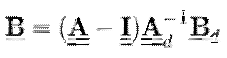
- B _ A _ _ ⁇ I _ _ A _ _ d ⁇ 1
- F _ A _ _ ⁇ I _ _ A _ _ d ⁇ 1 F _ _ d
- ⁇ t is the time interval between k and k + 1, k representing the portion of the control period and k + 1 the next portions.
- the matrix function expm() is the "matrix exponential" which can be calculated with standard methods (once only for fixed house parameters and time-step).
- the advantage of this formulation is that we can predict temperature evolution with a simple matrix multiplication.
- the duration of the control period is 24 hours and each portion is of 15 minutes' duration, so that k ranges from 1 to 96 inclusive.
- Cost Q ⁇ k Q k E E k + Q k T f T sp , k ⁇ T R
- f ( ⁇ T ) specifies the cost of an individual temperature's variation from set point.
- f ( x ) 0 ( x ⁇ 0):
- f ( x ) x ( x > 0)
- Q k E is the energy cost multiplier, i.e. the cost per unit energy
- Q k T is the comfort cost multiplier, i.e. the cost per degree-hour (if ⁇ t is measured in hours).
- Both of the costs and the set point can be specified for each time-step, to reflect variable energy tariff, or changes in desired comfort level through the day.
- the controller may set be set up so that, instead of inputting a comfort cost multiplier via the interface 12, the user simply specifies the ratio of the two multipliers as the cost is arbitrary to an overall multiplier; in this case one parameter Q E / Q T specifies the user's choice of comfort vs economy.
- Prior information required before optimisation is the initial state T 0 .
- the room temperature component of this will be measured, but the other components need to be estimated.
- a guess is adequate (radiator temperature is maybe 65° during heating, at room temperature otherwise; thermal mass temperature is the same as room temperature), but a better method is to use an observer such as a Kalman filter (just requires the state evolution equations above and estimates of process and measurement noise).
- T k + 1 A _ _ T k + B _ E k + 1 + F _ T E , k + 1
- the matrix (sizes are ), when expanded to show all the terms of A , B and F .
- T used in the expressions of E , and T o denotes the matrix transpose function, not that the matrix is raised to the power T.
- a To represents the initial conditions in the control period relates to the effect of operating the boiler at any stage in the control period on temperature at that and any subsequent stage in the control period, whilst accounts for the effects of external temperatures.
- minimising this functional involves adjusting each of the N dimensions of E to reduce the total cost.
- the rows of c correspond respectively to E >0, E ⁇ max, ⁇ > 0, ⁇ ⁇ T sp - T R .
- auxiliary variables ⁇ are required representing the temperature delta below set point.
- constraints for each time point:
- the optimum solution is calculated using a multi-dimension Newton gradient descent method, and the barrier functions gradually reduced as the solution becomes closer to optimum.
- the discomfort cost can be fixed as a linear matrix equation in E as:
- the house has a heat pump instead of a boiler, it is necessary to separate the power input to the plant (i.e. electricity) from the thermal energy delivered to the heating system, as their relationship varies quite a lot, and is highly dependent on the resulting system state (i.e. water temperature).
- the power input to the plant i.e. electricity
- the thermal energy delivered to the heating system as their relationship varies quite a lot, and is highly dependent on the resulting system state (i.e. water temperature).
- T R we can define (where the suffix H indicates e.g. with the rows relevant to the heating system pulled out, i.e. and write: (this is incidentally the same formulation that is required to implement a maximum heating system temperature constraint for the non-heat pump case).
- Water temperatures can change quite rapidly in the course of one time-step, and if the initial temperature is used in the constraint, the algorithm can fail to reflect the disadvantage of putting in high power, and so can be unstable to spikes.
- a solution for this is, whenever a water temperature is used in the update loop, to use the average 1 2 T k H + T k + 1 H (on the assumption that the water temperature increases linearly within the timestep) - and the same calculation with matrix is also used in the gradient.
- this approach may need alteration if applied to an air source heat pump with CO 2 refrigerant as it has different thermodynamics (i.e. the COP expression above is not valid).
- Each of the parameters can be thought of as a timescale or rate for:
- a _ _ d ⁇ r 1 ⁇ r 2 ⁇ r 3 r 1 r 3 r 4 ⁇ r 4 0 r 5 0 ⁇ r 5 ;
- B _ d 0 r 6 T 0 1 E max ;
- F _ d r 2 0 0 where ⁇ r 1 , r 2 , r 3 , r 4 , r 5 ⁇ are all positive rates and r 6 a positive heating rate. Note that in this notation we can just multiply r 6 T by [0...1] for the B E term according to the modulation level of the boiler.
- the six thermal parameters are determined from previously recorded data of the house's temperature and heat request inputs. There are a variety of methods of achieving this inference. Here we describe a simple and reasonably effective method for estimating these parameters. r 1 and r 2 are the only ones it is important to get right; estimates suffice for the others.
- the first column shows that energy input at the first time point has a bigger effect on the fourth time point than the first (representing system delays), and the zeros at the top right show that later energy inputs have no effect on earlier temperatures (as would be expected from causality).
- T superscript for the bracketed terms denote the transpose function
- R superscript for T the fact that is a T matrix of room temperature
- the Figure 4 shows the energy cost (solid line 28) and discomfort cost (dashed line 30) of this proposed solution as a function of time.
- the Total Cost is the sum of both of these over all time, which in this case is 2465.7 arbitrary units. Clearly this is not the optimal solution as all the cost is being incurred only for discomfort - we can inject energy to reduce this.
- the optimisation process is a way of adjusting the energy input to reduce the total cost.
- linear programming gradient descent, interior point method, primal-dual methods
- cost functional which can be differentiated twice, for a gradient vector and a Hessian matrix
- matrices expressing inequality constraints and optionally equality constraints
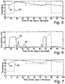
- Figures 5 and 6 show the optimised solution after solving for the minimum cost
- the graphs use the reference numerals of Figures 3 and 4 to denote corresponding lines.
- the energy cost directly indicates the energy input on a scale of 0 to 20.
- the cost as shown in Figure 6 can be seen to be fairly evenly distributed between Energy Cost 28 and Discomfort Cost now.
- the Total Cost is 575.5 arbitrary units, significantly reduced from the initial zero energy profile of the previous strategy.
- the energy usage is 4.52 hours of boiler firing energy.
- the boiler fires in advance of the first (evening) period of high set point (at 15 to 35 timesteps), getting the room to temperature in advance, but compromises slightly so that the room isn't quite to temperature at the start. It also doesn't fire for the second half of the period, letting the temperature ride to about 1 degree below set point - energy late at night is effectively expensive, as the heat is "wasted" when not needed overnight. For the following morning period, energy is saved by compromising on a lower temperature (there is little benefit from this energy as the period is so short), and the boiler firing is timed to give maximum benefit from this energy - just taking the chill off.
- the graph is representative of a system which is programmed to get the house to temperature in advance of a high set point period. Note that the method employed by the controller provides an automatic way (i.e. with no separate calculation required) of determining the optimum start time required to get a house to temperature in advance of a high set-point period.
- Figure 8 shows, for comparison, the theoretical performance of a conventional thermostat, programmed to turn the boiler on when the room temperature is below set point, together with some hysteresis.
- the solid line 24 is the room temperature predicted for this type of control, the broken line 26 being the set point schedule.
- FIG 8 An example of optimised heat pump control is shown in Figure 8 , we consider a variable electricity tariff - including a high price for weekday evenings (when demand on the grid is high) and a low price overnight. This is representative of a future grid demand-management scenario. We consider a two-day look ahead period.
- the cost multipliers Q E (solid) and Q T (dashed) are denoted by reference numerals 26 and 34 respectively.
- Figure 11 shows a number of energy and cost quantities for this solution: the input (electrical) power to the heat pump (solid line 40), the cost of this energy, i.e. multiplied by the tariff information Q E (dot-dashed line 42), the thermal power provided by the heat pump (dotted line 44), and the Discomfort Cost of this solution (dashed line 46).
- Figure 12 shows the anticipated flow temperature (radiator temperature) produced by the heat pump. Higher temperatures indicate less efficient running of the heat pump. This can be used to directly control the heat pump, if its interface enables specification of flow temperature.
- the heat pump has to work hard (and relatively inefficiently with a high flow temperature) to bring the room temperature up to the first high set point.
- a minimum flow temperature ( ⁇ 40degrees) is maintained statically (as in conventional heat pump control, but customised automatically to the house's thermal properties), until the high-demand period approaches.
- the control then ramps the heap pump power up, to generate enough heat to largely ride out the high-demand period with little further power required.
- Overnight the next lower set point period, starting at 100 time steps, the heat pumps runs quite hard to take advantage of cheap electricity.
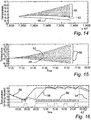
- Figures 13-16 graphically show the predictions that are made using the model to decide when is best to fire the boiler.
- Figure 13 below shows a decision to fire the boiler at the start of a "optimum start” period.
- the thick line 48 shows the target temperature profile produced by the optimisation calculations for the next half hour.
- the dashed lines 50 each show the predicted room temperature for a respective set of different control possibilities (firing now, firing later, together with turning off again at later times).
- the solid line 52 shows the closest fit to the temperature profile, and so this one is chosen. Since this prediction involved the boiler firing immediately, the boiler is turned on at this point.
- Figure 14 shows the opposite situation (using the same reference numerals for the corresponding lines): temperature is above the target temperature, and the chosen solution is to turn the boiler off immediately.
- Figure 15 shows an intermediate situation again using the same reference numerals as Figure 13 : the temperature profile is best matched by leaving the boiler on for a further 6 minutes, and then turning it off, and so no change is made to the boiler state at the present time.
- Figure 16 compares optimisation plus short term control with conventional thermostat control with hysteresis for a simulated house.
- the set point is shown by dashed line 54
- the room temperature achieved with the algorithm employed by the controller is shown by line 56
- the room temperature achieved by conventional control is shown by line 58
- the boiler firing requests from the control are shown by line 60
- the boiler firing request from the conventional control are shown in dashed lower line 62.
- the boiler cycles far more often, but at twice an hour this is still within the specification of normal boilers (typically four cycles per hour maximum) and will not impact appreciably on the boiler lifespan.
- the cycling is far less frequent than "chrono-proportional" control, which cycle the boiler six times per hour all the time (and achieve poorer temperature control).
- the algorithm knows exactly the best times to inject heat into the radiators (subject to some cycling time constraints) to achieve a target room temperature.
- This invention thus uses a model-based approach to predict an optimal "heating profile" according to the expected occupancy (expressed as a discomfort cost multiplier) of the house over the next day or longer: the best times to provide heat to the house given the occupiers' requirements.
- the strategy maintains the benefits of undershoot/overshoot correction, and eliminates the need to make detailed individual decisions about the heating strategy.
- the invention quantifies the trade-off between comfort and energy consumption, and uses a mathematical optimisation technique to calculate the heating profile (e.g. energy input at each minute of the day) that will minimise the net "Cost" of combined energy usage and occupier discomfort.
- the heating profile e.g. energy input at each minute of the day
- the technique is not restricted to this measure. Other factors such as the impact of cycling on the lifetime of the heating system can be factored into this Cost.
- the invention provides a methodology for calculating the best strategy for putting heat into a home (or other building), so that minimal energy is consumed for achieving occupant comfort.
- the learning calculations will be run continuously; the optimisation calculations are run periodically (e.g. every 15 minutes, looking ahead for the next day); and the short-term control is run continuously on controller 10, (e.g. every 2 minutes).
- the output of the optimisation calculations is a "heating strategy" consisting of how much power should be input to the heating system at each point in the optimisation period.
- the balance between the two “effective cost” figures determines whether the heating strategy is "economy” (for example, the homeowner is willing to have the temperature below set point for some of the day in order to save energy) or "comfort” (for example, the homeowner is willing to expend energy in order to ensure the house is always at their desired temperatures).
- additional blocks could be included, for example input from a solar thermal panel, or multiple rooms or zones within the house, or even domestic hot water requirements. This means the model can easily be extended to a wide range of system configurations using the same methodology.
- Non-linear blocks can also be included by linearising them within the optimisation loop (see below); for example a radiator does not strictly transfer heat directly proportional to temperature difference, but this can be represented as a local linear dependence near an approximate temperature.
- Storage heaters could be included by adding separate control variables for charging and discharging them, with their capacity modelled by a term similar to the heating system thermal mass.
- the optimisation is formed with the thermal energy output from the heat source as the variable parameter, which has a variable cost assigned to it dependent on the system state in the minimisation loop.
- the parameters of the thermal model of the house are typically unknown, and need to be learned from measurements made of the house's response to heat input (the techniques for carrying out this learning will be the subject of a future patent application). Nevertheless, even without learning, values can be estimated given the power of the heating system, the number of radiators, the size and build of the house.
- the prediction model is used to construct an expression for the Total Cost of a given heating strategy.
- Total Cost typically consists of (a) Energy Cost plus (b) Discomfort Cost (although the approach is not restricted to this type of Cost). Each of these is multiplied by a Cost coefficient - the balance between these determines whether we are in "comfort” or "economy” mode, as discussed in the Description section.
- the Total Cost is a function of the input power, but the effect on the heating system is a different quantity.
- the Energy Cost term is a function of the output heat (so for a heat pump the Energy Cost is the output heat divided by coefficient of performance).
- the Cost functional we include terms that result from the fact that changing temperatures within the system affect the Total Cost indirectly - the output heat is a function of the input power.
- the iteration loop processes impose constraints on the system variables (including but not restricted to):
- the iteration process can become unstable for non-linear systems.
- the solution is to use the average water temperature (or problematic variable) in the update loop, i.e. the average of the previous and next water temperatures, which ensures the Cost implications of a change are directly reflected.
- Step changes in variables (costs or constraints) can also cause instability in the optimisation process. This can be helped by using a smooth mathematical function that tends to the desired shape (e.g. piecewise linear) as another parameter goes to zero through the iterations, and with the use of "barrier functions" to represent constraints (with a weighting that goes to zero).
- a smooth mathematical function that tends to the desired shape (e.g. piecewise linear) as another parameter goes to zero through the iterations, and with the use of "barrier functions" to represent constraints (with a weighting that goes to zero).
- the future temperature is predicted, and compared with the heating profile.
- the option with a closest (e.g. least squares) match is chosen, and the boiler state changed if this option involves an immediate change to the boiler state.
- This approach applies the system wear Cost through fixed cycling time constraints - i.e. Infinite cost for exceeding these constraints.
- the approach can be extended by dynamically adjusting of the minimum times according to house thermal parameters and state, effectively taking account of a system wear Cost.
- a more sophisticated approach takes account of both types of cost directly (i.e. Cost of cycling and accuracy of meeting heating profile), and calculates the configuration of control outputs that minimise the resulting total cost.
- One specific example is as follows: Predicting 30 minutes ahead, compare the Cost of not changing the output state (i.e. on to off or vice versa) and changing the output state (once overall) at each 2 minute timestep in the 30 minute period.
- the Cost is the sum of the cost of a state change and the integrated cost of temperature inaccuracy during the period. If the option with the least Cost is to change the output state now, implement this.
- the Short-Term Control method is dependent on the physical system and being controlled and the interface available to it.
- Such systems include (but are not restricted to):
- Short-Term Control is not necessarily required; in some cases the output from the Optimisation step can be used directly as an output (e.g. control of return water temperature in heat pump).
Landscapes
- Engineering & Computer Science (AREA)
- General Engineering & Computer Science (AREA)
- Chemical & Material Sciences (AREA)
- Combustion & Propulsion (AREA)
- Mechanical Engineering (AREA)
- Physics & Mathematics (AREA)
- Signal Processing (AREA)
- Mathematical Physics (AREA)
- General Physics & Mathematics (AREA)
- Fuzzy Systems (AREA)
- Automation & Control Theory (AREA)
- Theoretical Computer Science (AREA)
- Human Computer Interaction (AREA)
- Computing Systems (AREA)
- Evolutionary Computation (AREA)
- Software Systems (AREA)
- Data Mining & Analysis (AREA)
- Computational Linguistics (AREA)
- Artificial Intelligence (AREA)
- Air Conditioning Control Device (AREA)
- Control Of Temperature (AREA)
Description
- This invention relates to a controller for a temperature management system, and to a method of controlling such a system.
- The invention is particularly applicable to temperature management systems, such as heating and/or air conditioning systems, that are used to control the temperature of one or more rooms in a building or other structure. The invention is more particularly, but not exclusively, concerned with domestic space heating systems and their control.
- Most domestic space heating systems control the temperature by targeting a set point temperature (which may form part of a schedule of set point temperatures that vary over a control period) and using a thermostat with hysteresis to turn the heat source on and off. This level of control is based only on the current state of the house and its heating system, and does not take into account any forward planning or knowledge of the thermal response of the house. Consequently, this known method of control can fail to achieve energy efficiency and/or the best comfort for the occupants of the house. For example, the room temperature is prone to fluctuate significantly under thermostatic control and can be uncomfortably low for the first part of a period with a raised set point temperature. Furthermore, if the set point temperature is raised for a relatively short period of time, this could result in further energy wastage as the temperature of the room increases gradually over that period, only reaching the vicinity of the set point temperature towards, or after, the end of the period of the raised set point temperature.
-
EP0688085 shows a temperature control system, in which known thermal properties of a building are used to predict temperatures which would be achieved by various possible energy inputs, and this information is used to formulate an energy input schedule that ensures that the building temperature does not fall below temperatures specified in a set point schedule. That schedule can exploit potential cost savings arising from a variable energy tariff, but can lead to room temperatures very much higher than the desired set point temperature, and cannot permit a compromise where the set point schedule would be even slightly violated in order to save energy. - Huval, B.; Barooah, P: "Optimization of a Heating System Using Smart Meters & Dynamic Pricing", University of Florida Undergraduate Honors Thesis, 341 August 2010, discusses predictive temperature management in which temperatures can deviate from a fixed deal temperature, but cannot accommodate a schedule of set temperatures.
- The present invention is defined in the appended claims.
- According to a first aspect of the invention, there is provided a controller for a temperature management system for heating and/or cooling a room in accordance with a schedule of set point temperatures over a control period, the controller comprising a data processor arrangement; a temperature input for receiving a signal indicative of the current temperature in the room; a control output for supplying control signals to the system; and at least one electronic memory for storing said schedule of set point temperatures, a relationship, based on known heating or cooling characteristics of the room, between the energy supplied to the system in a portion of the control period and the predicted temperature of the room during that portion and subsequent portions of the control period, a first parameter value representative of the cost of supplying said energy and a second parameter value representative of a predetermined acceptability of variations of the actual or predicted temperature of the room from the set point schedule, wherein processor arrangement is operable to calculate, for each said portion, the energy to be supplied to the system in order for a plurality of parameter values to satisfy a predetermined criterion, said plurality of parameter values comprising said first parameter value and said second parameter value.
- Thus a controller in accordance with the present invention can provide control for a temperature management system which not only takes into account the schedule of set point temperatures, but also a balance between the cost or notional cost of maintaining room temperature in accordance with the schedule and the effect of departures from that schedule. This enables the control of the temperature management system to be optimised so as to achieve the most effective use of energy to maintain the room at a comfortable temperature. The controller also takes into account the effect of an energy input in a given portion of the control period on the room temperature in that portion and also in subsequent portions of the period.
- The controller may to advantage be preprogrammed with said relationship between the energy supplied to the systems in a portion of the control period and the predicted temperature of the room during that and subsequent portions of the control period stored in the memory, and is preferably arranged for the user to enter the set point temperature schedule.
- Preferably, the criterion is applied to the sum of the parameter values.
- In this case, the criterion is preferably that the sum of the two values is substantially at a minimum.
- This enables the energy supplied to the system to be such that unnecessary heating/cooling, having regard to the acceptability (i.e. tolerance) defined by the second parameter value, can be avoided.
- The sum may, for example, be substantially at a minimum at the actual turning point defining the minimum or at an approximate minimum determined by an iterative process such as the gradient descent method or the Newton's method.
- Preferably, the approximate minimum is determined by the Primal-dual barrier function method.
- Preferably, the sum is of the values over the whole control period.
- Preferably, the data processor arrangement is operable to update said calculations for each of the portions over the course of the control period. This enables departures of the current temperatures from those previously predicted to be taken into account.
- The control period may conveniently be of 24 hours' duration, each portion being of 15 minutes' duration so that the period is constituted by 96 consecutive portions.
- The first parameter value comprises the product of the energy to be supplied to the system and an energy cost multiplier.
- This multiplier may vary over the course of the control period to take into account variations in the actual cost of consuming energy, as happens in the case of a smart grid electrical energy supply system, where the cost per unit of energy (usually electrical energy) supplied will vary or in the efficiency of the system, for example in the case of a heat pump, the efficiency of which will vary greatly with the temperature difference between the heat source and the heat sink of the pump.
- The second parameter value comprises the product of a comfort cost multiplier and the difference between the set point temperature and the actual or predicted temperature at the time. The second parameter value can thus be considered to be a discomfort cost.
- Thus, the second parameter value can be expressed as a discomfort cost, for example to an occupier of the room.
- The criterion, with these two types of parameter value may be that said total is minimised, subject to a fixed energy cost. Thus the user could specify the cost of energy to be consumed, and in response, the controller will determine a control schedule which achieves this with minimum discomfort cost.
- As with the cost multiplier for the first parameter value, the discomfort cost multiplier may vary over the course of a day/control period to account for, for example, levels of occupancy of the room, or the likely activity level of an occupant. Thus, the multiplier might be lower at night, when the occupant is in bed.
- Preferably, said relationship is based on a heat transfer model that takes into account at least one of:
- (a) the heat capacity and thermal transfer properties of the temperature management system;
- (b) the heat capacity and thermal transfer properties of the thermal mass of the room; and
- (c) the thermal transfer properties between the room and the external environment.
- Preferably, the properties listed at (c) above include the forecasted temperatures of the environment outside the room over the control period.
- The way in which the temperature management system is controlled to have the calculated amount of energy supplied to it may depend on the nature of the temperature management system itself. For example, where such a system comprises a boiler, the only type of allowable control of the boiler's operation may be switching the boiler (or its burner) on or off. However, in this case the controller may control the boiler by means of a suitable algorithm that simply turns the boiler on for a sufficient proportion of the portion for the calculated amount of energy for that portion to be supplied to, and hence consumed by, the boiler. For example the control system may supply the boiler with a control signal in the form of a series of pulses, each of which defines a period when the boiler is on. This signal can be pulse code modulated to provide short term control for the amount of energy delivered. Such modulation may be subject to conditions arising from operational constraints on the boiler, for example a minimum interval between successive activating pulses, to avoid damage or excessive wear to the temperature management system.
- Alternatively, however, the controller may be operable, during each portion, to use the predicted temperature profile associated with the calculated energy inputs as a target for the boiler and to compare this profile with further predicted temperatures for a part of the control period for different periods of activation or deactivation of the boiler's burner, an on-off control sequence being selected from a number of possible sequences to provide a profile of said further predicted temperatures that most closely matches the temperature profile.
- In this case the predicted temperature profile is used as an expression of the calculated amounts of energy to be supplied for each portion of the control period.
- According to a second aspect of the invention, there is provided a method of controlling a temperature management system for controlling the temperature of a room in accordance with the schedule of set point temperatures over a control period, the method comprising the steps of:
- (a) determining from known or predicted heating and/or cooling characteristics of a room a relationship between the series of predicted temperatures of the room in each of a succession of portions of the period and the energy supplied to the system in each of those portions; and
- (b) for each portion, using said relationship to calculate the amount of energy to be supplied in order for a first parameter value representative of the cost of supplying that energy and a second parameter value representative of a predetermined tolerance of variations of the predicted temperatures from the set point schedule to satisfy a predetermined criterion.
- The invention can more generally be seen as enabling the formulation of a control strategy for a system, which strategy balances one parameter value (for example a value related to the cost of operating the system) against another parameter value that has an antagonistic relationship to the first value (for example a cost attributable to the non-compliance of the system with a predetermined schedule).
- Thus the invention also lies in a controller for an apparatus management system for managing a quantitative characteristic of an apparatus in accordance with a schedule of set point values for the characteristic over a control period, the controller comprising an input for receiving data on the current value of said characteristic, a control output for supplying control signals to the system and at least one electronic memory for storing said schedule, a relationship between the control output in a portion of the control period and the predetermined value of the characteristic during that and subsequent portions of the control period, a first parameter value representative of the cost of energy supplied to or consumed by the system in response to said control signals and a second parameter value representative of the acceptability of variations of the actual or predicted value of the characteristic from the set point schedule, the controller further comprising a data processor arrangement which is operable to calculate, for each set portion, the energy to be supplied to or consumed by the system in order for a plurality of parameter values to satisfy a predetermined criterion, said plurality of parameter values comprising said first parameter value and said second parameter value.
- In the examples of the controller described and illustrated below, the characteristic is temperature and the first and second values are the energy and discomfort costs. However, the invention may be applied to other types of apparatus management systems, for example a plug-in series electric hybrid vehicle management system for controlling the amount of charge to be supplied to the batteries of the vehicle by the vehicle's internal combustion engine. In such a case, the first parameter value may comprise the cost of fuel consumed by the internal combustion engine, and the second value the acceptability of variations from the desired maximum speeds at which the vehicle may travel over the course of a journey.
- The invention will now be described, by way of example only, with a reference to the accompanying drawings in which:-
-
Figure 1 is functional block diagram illustrating the interaction between a controller in accordance with the invention and a house fitted with a boiler to be controlled by the controller; -
Figure 2 is a block diagram representation of a thermal model used, in effect, by the controller to predict future temperatures of the interior of the house in response to different energy inputs to the boiler; -
Figure 3 is a graph showing the predicted temperature of the house over a period of time and a schedule of set point temperatures in the situation in which no energy is delivered to the boiler i.e. there is no heating in the house; -
Figure 4 is a corresponding graph of the discomfort cost arising in those circumstances; -
Figure 5 is an example of the predicted temperature in a situation in which the controller has calculated the energy to be supplied to the boiler so as to minimise the sum of the energy cost and the discomfort cost; -
Figure 6 is a corresponding diagram showing the energy costs and the discomfort costs; -
Figure 7 shows, for the sake of comparison, a graph of predicted temperature if the discomfort cost were to be kept to the minimum; -
Figure 8 shows the predicted temperature for the situation which the control of a boiler corresponds to that provided by a conventional thermostat, programmed to turn the boiler on when room temperature is below the set point temperature (together with some hysteresis); -
Figure 9 is a graph showing energy and discomfort cost multipliers in a situation in which a heat pump is used to heat a house using electricity supplied under a tariff which varies over the control period; -
Figure 10 is a graph showing the temperature profile (and set point schedule) for a house heated by an air source heat pump, the control of which has been optimised by the controller according to the invention; -
Figure 11 is a graph showing a number of costs and energy quantities arising from the solution illustrated inFigure 10 ; -
Figure 12 shows the anticipated flow temperature (radiator temperature) produced by the heat pump controlled in accordance with the solution, the other effects of which are illustrated inFigures 10 and11 ; -
Figures 13-15 show how the controller can be used to provide short term control of the boiler in the house; and -
Figure 16 compares the control achieved by the controller, using the short term control, with the conventional thermostatic control (with hysteresis) for a boiler for a simulated house. - In
Figure 1 , the reference numeral 1 denotes a house having one ormore rooms 2 to be heated by a temperature management system comprising a boiler 4 linked to aheat delivery system 6 such as a set of radiators. Although the invention is described in relation to a boiler-based heating system, the benefits provided by the controller according to the invention are also applicable to other types of temperature management systems, in particular heat-pump based, heating and/or cooling systems. - A temperature sensor in the house (or a respective sensor in each room) is denoted by reference numeral 8 and feeds an output representative of the detected temperature to an
input 9 of acontroller 10 in accordance with the invention. Thecontroller 10 also has an input for control signals from auser interface 12 within the house 1. Theuser interface 12 can be used by a user to set up a schedule of set point temperatures over a control period (for example, a full day) and may also enable the user to specify the acceptability of variations from the set point temperature schedule, i.e. how hard the heating system has to work in order to strive to maintain the temperature within the room(s) of the house in accordance with the set point schedule. The acceptability parameter could be manifested as a comfort versus economy input value. The user may also specify that the acceptability of variations may itself change over the course of the control period. - The
controller 10 takes the form of a data processor arrangement comprising a computer programmed to perform the various tasks presented by functional blocks 14-17, and these are discussed below. It will be appreciated that the computer has an electronic memory on which said schedule is stored. The memory also stores data relating the energy supplied to/consumed by the boiler 4 in each portion of the control period to the temperature, predicted by the controller, during that portion and subsequent portions of the control period. In addition the computer memory stores first and second parameter values described above. Thecontroller 10 is also connected to anexternal computer network 19, such as the Internet, over which it obtains a forecast for the temperatures in the external environments (and optionally current temperature data) in the region of the house 1 over the course of the control period. The controller may receive further external temperature data from a localexternal temperature sensor 21 mounted on the exterior of the house 1, and directly connected to thecontroller 10. - Although the
controller 10 is shown outside of the house 1, it will be appreciated that in reality thecontroller 10 will be accommodated within the house. Thecontroller 10 has anoutput 18 over which it supplies control signals for switching the boiler 4 on and off. The functional control blocks 14-17 perform various data processing steps based on a thermal model of the house 1 as shown inFigure 2 . This model is used to relate the external temperature, TE, as forecast in the information obtained over thenetwork 19 and the energy to be supplied by the boiler 4 to the resultant room temperature TR in the house 1. The function represented by theblock 14 is the learning of the thermal properties of the house. One such property is the heat capacity of the room, i.e. the amount of heat energy required to raise the air temperature in the room by 1°C. The temperature in the room will also be influenced by the thermal mass within the room. Typically, the thermal mass will be primarily constituted by solid objects and/or surfaces within the room itself which are disconnected fromheat delivery system 6, but with which the room can exchange heat. Thelearning block 14 also includes the function of inferring the heat transfer characteristics between the room(s) and the outside world. Thus the functions represented by the block obtain the known heating and cooling characteristics of the room(s). - The
functional block 15 represents the initial estimate of the thermal state of the house at the start of a control period. The thermal state will be constituted by the air temperature of the room(s), TR, the temperature of theheat delivery system 6, TH, and the thermal mass temperature, TM. TR can be measured using the temperature sensor 8 whilst the other two temperatures can be estimated: TM can be treated as being the same as the room temperature (on the assumption that initially the house is in a steady state), whilst TH can be treated as being a predetermined temperature (e.g. the normal operating temperature of the radiators, say 65°C if the boiler 4 is operating, but room temperature otherwise). - The outputs from the learning and observation functions can be used to predict the effect of the energy supplied to the boiler during one portion of a trial period on the temperature of the room in that and in subsequent portions of the trial period. That effect can also be taken into account in the calculation of the effect of supplying energy during the next portion on the room temperature on the rest of the control period, and so on. The optimisation calculations that relate the energy to be supplied to the boiler to the resultant temperature profile of the room and, using inputs from the
interface 12 calculate a suitable energy input schedule, and the resultant predicted temperature profile for the room, are described below. In this particular instance, the output from the optimisation function is in the form of the calculated temperature profile which the short term control function uses to determine when to activate and deactivate the boiler 4 over the control period. The operation of, and theory behind, the calculations used by thecontroller 10 will now be described with further reference to the model shown inFigure 2 . - The optimisation calculations are based on a core model (for a "model predictive control" strategy).
-
Figure 2 is a simple physics model, with three blocks that can hold heat and transfer heat between each other. These are - (a) the heating system 6 (radiators, underfloor, etc) - which is directly heated by the heat plant;
- (b) the room 20 - which is heated by the heating system, and loses heat to the outside world; and
- (c) the remaining "disconnected"
thermal mass 22 of the house - which can exchange heat with the room (only). - Each of these has a heat capacity C (i.e. quantity of thermal material, taking a certain amount of energy to raise its temperature 7), and each link has a thermal conductance k. The heat capacities and thermal conductances constitute the known heating or cooling characteristics of the room.
- The energy flow between the blocks is represented by arrows.
- The physics can be written as three coupled linear differential equations for the conduction of heat between each block and the resulting change in temperature:


- There is an approximation here. Radiators (and also underfloor heating) transfer heat to the room by convection and radiation as well as conduction, which means there is a non-linear relationship between temperature difference and heat transfer. Nevertheless, we can regard the above equations as a linearised approximation around a "baseline" temperature difference, and iterative corrections can if necessary be made for the non-linearity.
- A matrix formulation means that the above equations can be more simply represented, and also provides an elegant framework for manipulating sets of temperatures - particularly when we need to manipulate time series of sets of temperatures. This approach is known as a "state space" formulation and is a more modern replacement for the more traditional "transfer function" approach to control theory.
- The differential equations above can be rewritten in matrix form as:


- The zeros arise from the assumption that there is no direct heat transfer between the heating system and the thermal mass of the house. In this case there are 6 independent parameters that describe our house model (whether or not the true boiler power is known).
- For short time periods, this can be used as a difference equation for updating the temperatures, but for longer time periods this will be inaccurate, and it is necessary to integrate the equation. This can be done analytically for a first order linear differential equation:


- In order to optimise heating control, a cost functional is required that reflects what we are trying to achieve. We wish to minimise energy consumption and discomfort; we assume that discomfort can be quantified by how much the temperature is below the user's setpoint. Hence (in discrete form):


- Both of the costs and the set point can be specified for each time-step, to reflect variable energy tariff, or changes in desired comfort level through the day. The controller may set be set up so that, instead of inputting a comfort cost multiplier via the
interface 12, the user simply specifies the ratio of the two multipliers as the cost is arbitrary to an overall multiplier; in this case one parameter QE /QT specifies the user's choice of comfort vs economy. - It would also be possible to include a penalty for being too much above a set point - for example some people like it to be cool at night - or an additional penalty for being too much below set point (e.g. "minimise my energy consumption but never let it be more that 2 degrees below set point"). The system design is scalable to including these new parameters.
- It will be appreciated that the superscripts E and T in equation (3) denote the energy and discomfort cost multipliers respectively, not Q raised to the power E or T.
- To calculate the optimal heating profile, we need to determine the {Ek } that minimises the cost Q. This is an N-dimensional minimisation problem, where N is the number of time-steps k we want to include.
- Prior information required before optimisation is the initial state T0. The room temperature component of this will be measured, but the other components need to be estimated. A guess is adequate (radiator temperature is maybe 65° during heating, at room temperature otherwise; thermal mass temperature is the same as room temperature), but a better method is to use an observer such as a Kalman filter (just requires the state evolution equations above and estimates of process and measurement noise).
- We can express the temperature state at each of N times in the future as a linear matrix function of the energy input at each time in the future. Specifically, from the equation constructed above:

- We start from k = 0 (T0 is our known initial state):


- This allows us to write a matrix expression for the temperature states at every time as a function of the initial temperature state, and the energy input and external temperature at every time step. Explicitly, this uses the following matrices (constructed iteratively and representing the forward propagation of the predictions of the model):


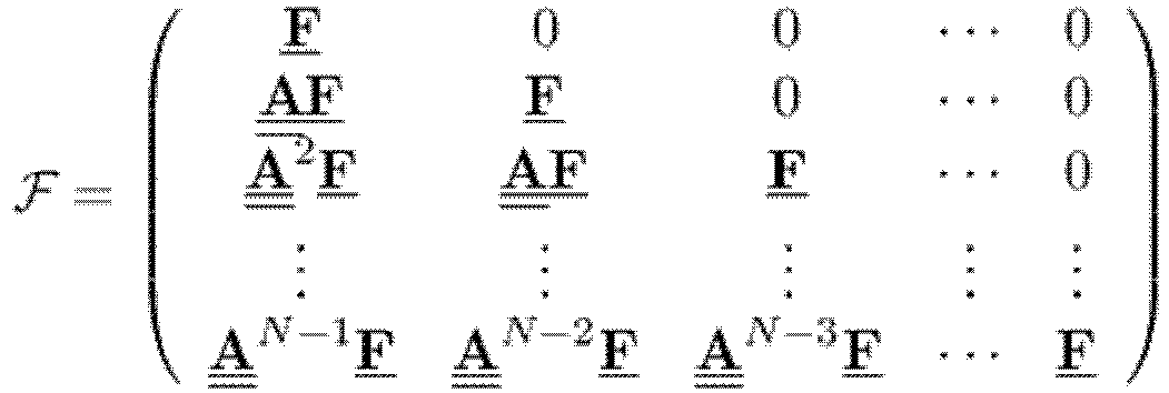
- The matrix (sizes are

- The set of temperature predictions for the time period

- These can be calculated from the initial conditions, energy input E = (E 1, E 2,...EN )T and external temperatures using these matrices as:

 relates to the effect of operating the boiler at any stage in the control period on temperature at that and any subsequent stage in the control period, whilst
 accounts for the effects of external temperatures.
- All the matrices above are a little complex to use as they contain predictions for all three model temperatures. Most of the time we just want to see the effect of energy on room temperature, and for this we pick out selected rows. If we use the superscript R to indicate the rows in the matrices corresponding to room temperatures R, i.e. rows 1, 4, 7,...3N - 2 we can write the room temperature as:


- We define


- The aim now is to calculate the vector of energy inputs E that minimises the cost Q(E) subject to a number of constraints. There are many established techniques for solving this type of problem, and we can formulate it in the standard form:
- Minimise Q(E) subject to c(E) ≥ 0 and g(E) = 0
- Intuitively, minimising this functional involves adjusting each of the N dimensions of E to reduce the total cost.
- We consider below three different methods for solving the optimisation problem.
- This method requires that Q, c and g are linear. This means the function f must be piecewise linear. We consider the simple case described after Eqn 3: f(x) = 0 (x < 0); f(x) = x (x > 0), and to that end we need to introduce a vector of auxiliary variables ε ≥ T sp - TR . Now we can write:


- The rows of c correspond respectively to E>0, E<max, ε > 0, ε ≥ T sp - TR.
- (Note that this excludes for simplicity constraints on the maximum temperature of the heating system which can be achieved by adding a further set of rows to a and b similarly to the last above.).
- These matrices can be passed straightforwardly to the Octave interface1 to GLPK2 with the following syntax

- This method no longer requires that Q(E) is linear and so enables solution of heat pump control problems (see section below) and non-linear cost functions (e.g.f). The method is intuitive but is slow in the vicinity of constraints, which are better dealt with by a barrier function method (see below), but it provides an easily describable algorithm for the non-linear case.
- For gradient descent we also need to calculate the gradient ∇Q. For the simple linear f form off this is:

- The idea is that E is always adjusted in the multi-dimensional direction which will reduce Q best.
1 http//www.gnu.org/software/octave/doc/interpreter/Linear-Programming.html
2 http//www.gnu.org/software/glpk/ - The optimisation algorithm for gradient descent is as follows:
- 1. Decide on Δt N; determine house thermal parameters (see learning below); pre-calculate and Toffset; get future set points and external temperature forecast.

- 2. Determine the initial internal state T 0 (by guess or Kalman filter)
- 3. Decide on an initial guess of the energy input profile E (suggested to be very small but not quite zero)
- 4. Calculate the gradient (above).
- 5. Adjust the energy with a multiple of the gradient: E → E - α∇Q using α sufficiently small that constraints are not violated
- 6. Calculate the resulting water temperature, and reduce the relevant entries Ej so that they are (a) below or equal to the maximum boiler output power and (b) so that the water temperature doesn't exceed maximum; recalculate temperature profiles.
- 7. Iterate back to step 4 until some stopping criterion reached (e.g. cost no longer reducing much, or fixed number of iterations).
- This method has two significant advantages over the gradient descent method: constraints are dealt with elegantly and efficiently, and the full Newton's method can be used to improve convergence speed. Non-linear cost functions are supported. This is the method we have found to work best, and is still a standard method in the scientific literature3.
- Similarly to the linear programming method, auxiliary variables ε are required representing the temperature delta below set point. There are five constraints (for each time point):
- 1. ε greater than or equal to zero
- 2. ε greater than or equal to temperature delta below set point
- 3. System water temperature less than maximum value
- 4. Energy input greater than or equal to zero
- 5. Energy input less than maximum
- For each of these we introduce a logarithmic barrier function multiplied by a single common variable µ, together with a dual variable (Lagrange multiplier) for each dimension of each constraint. We also need the ability to calculate the Hessian matrix of the cost Q with respect to the energy inputs E.
- The optimum solution is calculated using a multi-dimension Newton gradient descent method, and the barrier functions gradually reduced as the solution becomes closer to optimum.
- The steps in this algorithm are as follows:
- 1. Construct initial system matrices as previously, including constraint matrices
- 2. Make an initial guess for energy input (either from previous time-step or near zero), and barrier multiplier µ
- 3. Calculate cost and cost gradient
- 4. Either (a) continue line search in current direction or (b) calculate descent direction according to the interior point method, and choose a multiplier α small enough that constraints are satisfied.
- 5. Calculate new energy input
- 6. If change since last time is sufficiently small, reduce µ .
- Finish if µ is sufficiently small (and change since last time was sufficiently small), otherwise iterate back to Step 3.
- The standard barrier function (or interior point) method additionally allows for the specification of equality constraints in the form of the matrix equation Ax = b, through the addition of further Lagrange multipliers and some extensions to the internal formulation. This provides a straight-forward means of specifying a fixed energy E total such that ∑ iEi = E total, and using the above optimisation to calculate the optimal distribution of the energy. Alternatively, the discomfort cost can be fixed as a linear matrix equation in E as:

- The linear programming method above can be easily adapted for the fixed energy inputrequirement. We redefine the matrices a and b so that there is an additional row specifying the equality constraint on the total energy (being the sum of the elements of E):

= glpk (, , , [], [], "LL...LS", "CC...CC", 1). - If the house has a heat pump instead of a boiler, it is necessary to separate the power input to the plant (i.e. electricity) from the thermal energy delivered to the heating system, as their relationship varies quite a lot, and is highly dependent on the resulting system state (i.e. water temperature).
- Our model for an air source heat pump is that the thermal power E provided by the heat pump when driven by electrical power P is

- To carry out the optimisation it is necessary to work with the thermal power E as our variable as otherwise the propagation step (calculating) becomes non-linear and potentially time-consuming. The energy cost term is dependent on P not E so


- This equation is missing a particular subtlety: We need the dependence of Q on E, but the heating system temperature

- As previously for TR , we can define
 with the rows relevant to the heating system pulled out, i.e.


- Hence, we can write Q with its full dependence on E shown explicitly:

- This method requires an explicit function for the gradient of Q with respect to E. This is slightly simplified if we note that


- It will be appreciated that we are, in effect, performing matrix multiplications using indices to take care of which time step we're comparing with which.characterises the effect of E on water temperature, and
 characterises its effect on room temperature.
- We can use this gradient within the same algorithm described above, taking care of the difference between electrical power provided to the heat pump and its output power. The heat pump's output power is constrained by a direct limit on the input power and so this limit must be updated each loop according to the current water temperatures. Similarly the heat pump has a maximum water temperature it can deliver (typically 60°).
- Water temperatures can change quite rapidly in the course of one time-step, and if the initial temperature is used in the constraint, the algorithm can fail to reflect the disadvantage of putting in high power, and so can be unstable to spikes. A solution for this is, whenever a water temperature is used in the update loop, to use the average
 is also used in the gradient.
- Extension to a ground source heat pump is fairly straight forward - just replace the forecast air temperature TE with the forecast temperature of the ground loop.
- On a similar note, this approach may need alteration if applied to an air source heat pump with CO2 refrigerant as it has different thermodynamics (i.e. the COP expression above is not valid).
- The differential equations used to describe our model of the house are expressed as matrices A d , B d , F d , for use within the subsequent calculations. We can identify six independent parameters as making up these matrices, as described below.
- Each of the parameters can be thought of as a timescale or rate for:
- 1. Room temperature to be affected by heating system: r 1 = 1/τRH = kH /CR (approx how quickly room warms up if radiators at const temp and no delta to outside)
- 2. Room temperature to be affected by external temperature: r 2 = 1/τRW = kW /CR (approx how quickly room cools down when heating off -- outflow)
- 3. Room temperature to be affected by thermal mass: r 3 = 1/τRM = kM /CR (approx how quickly room heats from thermal mass)
- 4. Heating system to be affected by room temperature: r 4 = 1/τHR = kH /CH (approx how quickly radiators cool)
- 5. Thermal mass to be affected by room temperature: r 5 = 1/τMR = kM /CM (approx how quickly thermal mass charges/discharges)
- 6. Rate of change of temperature of heating system at given thermal energy input:

- These are all exponential timescales.
- Hence we can write


- Note that our method is not specific to these parameters - we can include an arbitrary number of blocks in our thermal model of the house - this is just a relatively simple example. The method would also work just as well excluding the radiator or thermal mass components of the model, although of course the match to reality would be less good.
- The six thermal parameters are determined from previously recorded data of the house's temperature and heat request inputs. There are a variety of methods of achieving this inference. Here we describe a simple and reasonably effective method for estimating these parameters. r 1 and r 2 are the only ones it is important to get right; estimates suffice for the others.
- 1. Determine r 2: identify a period of time (e.g. overnight) when there has been no heat input for several hours and it is at least 5 degrees cooler outside. The radiators will be at the same temperature as the room and we assume that the thermal mass is the same temperature also. Therefore

- 2. Determine r 1: identify a period of continuous heating when the heat has been on for at least 30 minutes. At this point the radiators will have reached their maximum temperature and we assume that the thermal mass is the same temperature as the room. Therefore (from above)

- 3. Estimate r 4 by looking at overshoot: after the heating has been on for an extended period, look at how long it takes for the room temperature and start falling again. r 4 is approximately the inverse of this timescale.
More accurately, simulate room temperature evolution with r 1 and r 2 in place, and adjust r 4 to match the amount of room temperature overshoot after an extended heating period. Analytic expressions are also possible but they are complex. - 4. Estimate r 6 by looking at how long it takes before the room temperature is increasing at its maximum rate at the start of an extended heating period. This time, t inc, is approximately the time for the boiler to reach its maximum temperature, and so r 6 = (TH - TR )/t inc ≃ 45/t inc (in e.g. degrees per hour).
- 5. Estimate r 3 and r 5 according to the thermal mass of the property. These do not matter greatly and values in the range 1/(8-24hours) are usually right.
- An example set of sensible parameters (in units of per hour, or degrees per hour for r 6) are these (learned from the author's house):

- Using a house model with parameters (for time measured in hours, and temperature in degrees C)


- Integrating these for a timestep of 15 minutes yields


- We can now construct propagation matrices. Considering 24 hours ahead at 15 minute steps, gives 96 × 96 matrices. Demonstrating this for room temperature, we construct
 (96 × 96) such that

- For
initial temperatures 


- The annexed spreadsheet (Annex) shows further information in detail:
- Set point of 15 changing to 19, 5, 19 and back to 15
- Energy cost QE of 10 (constant)
- Temperature cost QT of 0.5 (constant)
- If the temperature cost function f(ΔT) = ΔT + 2(ΔT)2 and we also apply a heating system maximum temperature constraint of 70° C then the optimised energy input (limited to between 0 and 1) is:


- The T superscript for the bracketed terms denote the transpose function, the R superscript for T the fact that is a T matrix of room temperature.
- Examples of further heating, energy input and discomfort profiles are discussed below with reference to
Figures 3 to 12 . - We choose an energy cost of 20 (units per 15mins at full capacity) and a temperature cost of 1 (units per 15 mins per degree below set point) - this is an "economy" setting with a big energy penalty. We also choose a slightly non-linear (quadratic) cost function to achieve better performance.
- We can now plot graphs of heating profiles and their costs.
Figure 3 shows a solution of zero energy input, thesolid line 24 room temperature
trace 26 the set point profile (red dashed) being used for this optimisation calculation:
The temperature is just allowed to decay as no heat is provided to the (simulated) property. - The
Figure 4 shows the energy cost (solid line 28) and discomfort cost (dashed line 30) of this proposed solution as a function of time. - These incorporate both the multipliers Q and the cost functions of energy and temperature difference.
- The Total Cost is the sum of both of these over all time, which in this case is 2465.7 arbitrary units. Clearly this is not the optimal solution as all the cost is being incurred only for discomfort - we can inject energy to reduce this.
- The optimisation process is a way of adjusting the energy input to reduce the total cost. There are published methods for this (linear programming, gradient descent, interior point method, primal-dual methods), given a cost functional (which can be differentiated twice, for a gradient vector and a Hessian matrix) and matrices expressing inequality constraints (and optionally equality constraints). Hence we do not describe these steps in detail as the intricacies are not novel.
-
Figures 5 and 6 show the optimised solution after solving for the minimum cost, the graphs use the reference numerals ofFigures 3 and 4 to denote corresponding lines. - Note that the energy cost directly indicates the energy input on a scale of 0 to 20.
- The cost as shown in
Figure 6 can be seen to be fairly evenly distributed betweenEnergy Cost 28 and Discomfort Cost now. The Total Cost is 575.5 arbitrary units, significantly reduced from the initial zero energy profile of the previous strategy. The energy usage is 4.52 hours of boiler firing energy. - The boiler fires in advance of the first (evening) period of high set point (at 15 to 35 timesteps), getting the room to temperature in advance, but compromises slightly so that the room isn't quite to temperature at the start. It also doesn't fire for the second half of the period, letting the temperature ride to about 1 degree below set point - energy late at night is effectively expensive, as the heat is "wasted" when not needed overnight. For the following morning period, energy is saved by compromising on a lower temperature (there is little benefit from this energy as the period is so short), and the boiler firing is timed to give maximum benefit from this energy - just taking the chill off.
- To further see the benefits of the controller of the invention, we can compare the heating profile of
Figure 5 with two alternative strategies for heating the home. - Firstly, a "comfort" setting where no compromise is allowed. We can calculate this in the same way as above, but with a very low Energy Cost multiplier. This results in a profile as shown in
Figure 7 (which uses corresponding reference numerals to those ofFigure 5 ). - This uses 7.18 hours of boiler firing energy - nearly 60% more for (subjectively) disproportionately little benefit to the consumer - although this is a demonstration rather than an energy savings claim. The graph is representative of a system which is programmed to get the house to temperature in advance of a high set point period. Note that the method employed by the controller provides an automatic way (i.e. with no separate calculation required) of determining the optimum start time required to get a house to temperature in advance of a high set-point period.
-
Figure 8 shows, for comparison, the theoretical performance of a conventional thermostat, programmed to turn the boiler on when the room temperature is below set point, together with some hysteresis. In this case thesolid line 24 is the room temperature predicted for this type of control, thebroken line 26 being the set point schedule. - This uses 5.57 hours of boiler firing energy (more than our economised control), but very little of the benefit is seen by the consumer - most of the warmth occurs after they have gone to bed (timestep 40) or when they don't need it (at the end of the time period when the set point is quite low). The Discomfort Cost is high also, as the room is mostly below set point during the higher set point periods.
- An example of optimised heat pump control is shown in
Figure 8 , we consider a variable electricity tariff - including a high price for weekday evenings (when demand on the grid is high) and a low price overnight. This is representative of a future grid demand-management scenario. We consider a two-day look ahead period. The cost multipliers Q E (solid) and Q T (dashed) are denoted byreference numerals - The solution of the optimisation problem for an air-source heat pump (for a house with specific thermal parameters) is shown on the graph of
Figure 10 below, with room temperature (solid line 36) and the input set point profile (dashed line 38). -
Figure 11 shows a number of energy and cost quantities for this solution: the input (electrical) power to the heat pump (solid line 40), the cost of this energy, i.e. multiplied by the tariff information Q E (dot-dashed line 42), the thermal power provided by the heat pump (dotted line 44), and the Discomfort Cost of this solution (dashed line 46). -
Figure 12 shows the anticipated flow temperature (radiator temperature) produced by the heat pump. Higher temperatures indicate less efficient running of the heat pump. This can be used to directly control the heat pump, if its interface enables specification of flow temperature. - At the start, the heat pump has to work hard (and relatively inefficiently with a high flow temperature) to bring the room temperature up to the first high set point. During the next period, a minimum flow temperature (∼40degrees) is maintained statically (as in conventional heat pump control, but customised automatically to the house's thermal properties), until the high-demand period approaches. The control then ramps the heap pump power up, to generate enough heat to largely ride out the high-demand period with little further power required. Overnight (the next lower set point period, starting at 100 time steps), the heat pumps runs quite hard to take advantage of cheap electricity. Finally, during the unoccupied period (around 150 timesteps) the heat pump gradually ramps its power up - this is a novel heat pump control strategy, as conventionally heat pumps are either run continuously overnight, or are turned off for a crude set-back. At the end, the temperature is allowed to fall off as no future periods are (yet) in sight.
- All of the above decisions are determined automatically from the optimisation process, for the whole period at once; at best, conventional heuristic algorithms would have to make each decision individually.
- To illustrate short term control,
Figures 13-16 graphically show the predictions that are made using the model to decide when is best to fire the boiler. - Firstly,
Figure 13 below shows a decision to fire the boiler at the start of a "optimum start" period. Thethick line 48 shows the target temperature profile produced by the optimisation calculations for the next half hour. The dashedlines 50 each show the predicted room temperature for a respective set of different control possibilities (firing now, firing later, together with turning off again at later times). Thesolid line 52 shows the closest fit to the temperature profile, and so this one is chosen. Since this prediction involved the boiler firing immediately, the boiler is turned on at this point. -
Figure 14 shows the opposite situation (using the same reference numerals for the corresponding lines): temperature is above the target temperature, and the chosen solution is to turn the boiler off immediately. -
Figure 15 shows an intermediate situation again using the same reference numerals asFigure 13 : the temperature profile is best matched by leaving the boiler on for a further 6 minutes, and then turning it off, and so no change is made to the boiler state at the present time. -
Figure 16 compares optimisation plus short term control with conventional thermostat control with hysteresis for a simulated house. The set point is shown by dashedline 54, the room temperature achieved with the algorithm employed by the controller is shown byline 56, the room temperature achieved by conventional control is shown byline 58, the boiler firing requests from the control are shown byline 60 and the boiler firing request from the conventional control are shown in dashedlower line 62. - It can be seen that far tighter control of the smoothing band is achieved with our algorithm, in this case achieving sub-noise level smoothing (which would be impossible with any hysteresis approach). The benefit of this is that the house is always at the required temperature: there is better consumer comfort and no energy is wasted getting the room unnecessarily warm. Whereas the final fire of the conventional control is largely "wasted", the algorithm used by the controller does not heat the room any more than necessary at the end of the high set point period.
- The boiler cycles far more often, but at twice an hour this is still within the specification of normal boilers (typically four cycles per hour maximum) and will not impact appreciably on the boiler lifespan. The cycling is far less frequent than "chrono-proportional" control, which cycle the boiler six times per hour all the time (and achieve poorer temperature control).
- In summary, through the explicit house model, the algorithm knows exactly the best times to inject heat into the radiators (subject to some cycling time constraints) to achieve a target room temperature.
- This invention thus uses a model-based approach to predict an optimal "heating profile" according to the expected occupancy (expressed as a discomfort cost multiplier) of the house over the next day or longer: the best times to provide heat to the house given the occupiers' requirements. The strategy maintains the benefits of undershoot/overshoot correction, and eliminates the need to make detailed individual decisions about the heating strategy.
- The invention quantifies the trade-off between comfort and energy consumption, and uses a mathematical optimisation technique to calculate the heating profile (e.g. energy input at each minute of the day) that will minimise the net "Cost" of combined energy usage and occupier discomfort. In the described examples of quantifiable discomfort is the amount of time that the temperature is below a desired set point (Cost measured in degree-hours), but the technique is not restricted to this measure. Other factors such as the impact of cycling on the lifetime of the heating system can be factored into this Cost.
- Three applications of this optimisation approach may be particularly beneficial:
- 1) Underfloor heating. Controlling an underfloor heating system can be difficult; there is a large thermal inertia from the storage of heat in the physical fabric of the building, and hence energy input needs to be planned many hours in advance. This invention means that the thermal mass of the floor can be explicitly taken into account, and the minimal amount of energy can be injected at the right time to achieve occupant comfort.
- 2) Heat pumps. Ground-source and air-source heat pumps are one of the most carbon-efficient means of heating a house, but many installations are not as effective as they could be due to poor controls and configuration. The efficiency of a heat pump depends strongly on the temperature of the water it is delivering, so there is a big incentive to run the heat pump as cool as possible. A heat pump is conventionally controlled by running it all the time to achieve a target water temperature, with a simple linear compensation for external temperature. This approach is inflexible (and thus energy-inefficient) and susceptible to misconfiguration. The approach described in this invention avoids these pitfalls by using a model-based predictive control strategy.
- 3) Smart grids. It is becoming increasingly important to adjust electric grid load according to demand. This invention provides an energy-efficient strategy to support the smart grid with minimal impact on a householder. Advanced knowledge of a period of high grid demand and thus high energy cost can be incorporated in the optimisation calculation for an electric heating system (e.g. a heat pump or storage heater), and the energy profile will be adjusted to achieve comfort at minimal cost, for example increasing heat output before turning the heating system off during a period of high demand.
- The invention provides a methodology for calculating the best strategy for putting heat into a home (or other building), so that minimal energy is consumed for achieving occupant comfort.
- To utilise Optimised Heating in practice, three stages are involved:
- 1) Learning the thermal parameters of the house: over a period of several weeks these characteristics can be deduced from sensor measurements. The exact method for this process is not included in the present invention. The controller can work effectively with preset parameters given knowledge of the house type, construction etc.
- 2) Optimisation of the heating strategy for period of time in the future (for example looking a day or two ahead). This is the core of the invention.
- 3) Short-term control to use the heating strategy to control a real heating system: decisions in real time as to when to fire a boiler or what power level to run a heat pump at.
- The learning calculations will be run continuously; the optimisation calculations are run periodically (e.g. every 15 minutes, looking ahead for the next day); and the short-term control is run continuously on
controller 10, (e.g. every 2 minutes). - To run the optimisation calculations, the following inputs are used:
- Model for the house's thermal properties and heating system (e.g. boiler, heat pump), possibly learned. The model is described in more detail in the next section.
- Set point schedule for occupant's desired temperature over the optimisation
- External temperature forecast for the optimisation period (received over the internet by the "hub", or an estimate based on the time of year, etc.).
- Effective "cost" of energy supplied to the heating system, including any variations in tariff over the optimisation period.
- Effective "cost" of occupant discomfort, such as a figure in degree-hours for the room temperature being below (or above) each set point in the schedule period. This could consist of three different temperatures for scheduled "in", "out" and "asleep" periods; more complex variations in temperature can be handled easily.
- The output of the optimisation calculations is a "heating strategy" consisting of how much power should be input to the heating system at each point in the optimisation period.
- The balance between the two "effective cost" figures determines whether the heating strategy is "economy" (for example, the homeowner is willing to have the temperature below set point for some of the day in order to save energy) or "comfort" (for example, the homeowner is willing to expend energy in order to ensure the house is always at their desired temperatures). With regard to the model shown in
Figure 2 , additional blocks could be included, for example input from a solar thermal panel, or multiple rooms or zones within the house, or even domestic hot water requirements. This means the model can easily be extended to a wide range of system configurations using the same methodology. Non-linear blocks can also be included by linearising them within the optimisation loop (see below); for example a radiator does not strictly transfer heat directly proportional to temperature difference, but this can be represented as a local linear dependence near an approximate temperature. Storage heaters could be included by adding separate control variables for charging and discharging them, with their capacity modelled by a term similar to the heating system thermal mass. - When the heat source is non-linear (as in the case of a heat pump the optimisation is formed with the thermal energy output from the heat source as the variable parameter, which has a variable cost assigned to it dependent on the system state in the minimisation loop.
- The parameters of the thermal model of the house are typically unknown, and need to be learned from measurements made of the house's response to heat input (the techniques for carrying out this learning will be the subject of a future patent application). Nevertheless, even without learning, values can be estimated given the power of the heating system, the number of radiators, the size and build of the house.
- In the described examples, the prediction model is used to construct an expression for the Total Cost of a given heating strategy. Total Cost typically consists of (a) Energy Cost plus (b) Discomfort Cost (although the approach is not restricted to this type of Cost). Each of these is multiplied by a Cost coefficient - the balance between these determines whether we are in "comfort" or "economy" mode, as discussed in the Description section.
- Energy Cost is (for example) the total energy input over the period. The effective cost of energy can be a financial cost and reflect the energy tariff - and thus can vary throughout the optimisation period, thus supporting smart grids or fixed tariff hours.
- Discomfort Cost is (for example) incurred when the temperature is below (or above) the given set points, measured as the integrated temperature difference to the set point. The function can be nonlinear in temperature - for example, to reflect that 2 degrees below set point is more than twice as bad as 1 degree below. Note that the time points where Discomfort Cost is incurred are on the "output" side of the matrix, so the Cost consequences of an energy input are incurred at all subsequent timesteps.
- For a non-linear heat source such as a heat pump, the Total Cost is a function of the input power, but the effect on the heating system is a different quantity. We rewrite the Energy Cost term as a function of the output heat (so for a heat pump the Energy Cost is the output heat divided by coefficient of performance). When we differentiate the Cost functional (with respect to input power) we include terms that result from the fact that changing temperatures within the system affect the Total Cost indirectly - the output heat is a function of the input power.
- This approach is applicable to air source heat pumps, ground source heat pumps, air to-air heat pumps (and air conditioners), or any other non-linear heat source.
- For a heat source such as an air-source heat pump which is dependent on external weather (e.g. air temperature), the approach enables optimised use given weather forecast (e.g. running the heat pump more during the day when it is warmer and thus more efficient).
- Some modern heat pumps utilise different thermodynamics (e.g. CO2 refrigerant) and thus perform differently from normal heat pumps; a thermodynamic model for this can be included straight-forwardly in this methodology, with improved optimisation for these heat pumps.
- The iteration loop processes impose constraints on the system variables (including but not restricted to):
- A maximum power for the heating system (for a non-linear heat sources such as a heat pump this affects the input power not the output power)
- A maximum water temperature (perhaps 70° for a conventional boiler, or 60° for a heat pump)
- Constraints on dependent variables (e.g. temperatures) can be applied with additional terms in the Cost functional.
- If the heating system has large changes during a timestep, the iteration process can become unstable for non-linear systems. The solution is to use the average water temperature (or problematic variable) in the update loop, i.e. the average of the previous and next water temperatures, which ensures the Cost implications of a change are directly reflected.
- Step changes in variables (costs or constraints) can also cause instability in the optimisation process. This can be helped by using a smooth mathematical function that tends to the desired shape (e.g. piecewise linear) as another parameter goes to zero through the iterations, and with the use of "barrier functions" to represent constraints (with a weighting that goes to zero). We have found that the method that works well in practice is a primal-dual interior point method with logarithmic barrier functions; this can reliably inequality constraints, equality constraints, and non-linearity.
- This approach with prediction model matrices and a Cost functional can also be used for other requirements:
- Calculating the heating strategy for a fixed energy consumption in the optimisation period - i.e. how to distribute the available energy through the period in order to maximise comfort. This enables a home-owner to specify their spend on heating instead of using a thermostat directly. In this scenario the set point becomes the cut-off where there is no advantage to the homeowner in the temperature being higher (lower) than it.
- Calculating the heating strategy that minimises energy for a fixed level of comfort, if this is the user requirement rather than the Total Cost of both together.
- Both of these require the specification of equality constraints within the optimisation problem.
- The Optimisation calculations are run frequently enough that many changes can be reacted to as part of that, and Short-Term Control can be regarded as finding the best method of distributing the power throughout the optimisation time-step given the physical limitations of the heating system.
- One specific approach for Short-Term Control is for an on-off controller as follows:
- 1. Specify a minimum complete cycle time (e.g. 30 minutes) and a minimum change time (e.g. 5 minutes). If these times are not exceeded, do not change the boiler state.
- 2. If the boiler is currently off and the heating profile (optimisation output) indicates no heat is required immediately, keep the boiler off.
- 3. If the boiler is currently on and the heating profile indicates full boiler power is required, keep the boiler on.
- 4. Otherwise, look ahead a period of time (e.g. 30 minutes) and consider the following possibilities (within the constraints in 1.):
- (a) not changing the boiler state at all
- (b) changing the boiler state at a number of time delays after the present time
- (c) changing the boiler state immediately, and changing it back after a number of time delays after the present time.
- For each of these the future temperature is predicted, and compared with the heating profile. The option with a closest (e.g. least squares) match is chosen, and the boiler state changed if this option involves an immediate change to the boiler state.
- This approach applies the system wear Cost through fixed cycling time constraints - i.e. Infinite cost for exceeding these constraints. The approach can be extended by dynamically adjusting of the minimum times according to house thermal parameters and state, effectively taking account of a system wear Cost.
- A more sophisticated approach takes account of both types of cost directly (i.e. Cost of cycling and accuracy of meeting heating profile), and calculates the configuration of control outputs that minimise the resulting total cost.
- One specific example is as follows:
Predicting 30 minutes ahead, compare the Cost of not changing the output state (i.e. on to off or vice versa) and changing the output state (once overall) at each 2 minute timestep in the 30 minute period. The Cost is the sum of the cost of a state change and the integrated cost of temperature inaccuracy during the period. If the option with the least Cost is to change the output state now, implement this. - The Short-Term Control method is dependent on the physical system and being controlled and the interface available to it. Such systems include (but are not restricted to):
- Conventional boiler control (on or off; self modulating)
- Direct control of modulation level of boiler (e.g. through OpenTherm interface)
- Heat pump: direct on/off control of unmodulating compressor
- Heat pump: direct control of power level of modulating compressor
- Heat pump: control of return water temperature (self-modulating)
- Heat pumps: overall on/off control (when internal control strategy of heat pump known)
- Short-Term Control is not necessarily required; in some cases the output from the Optimisation step can be used directly as an output (e.g. control of return water temperature in heat pump).
Margaret H. Wright (2005). "The interior-point revolution in optimization: history, recent developments, and lasting consequences". Bull. Amer. Math. Soc. (N.S), .
Bonnans, J. Frédéric; Gilbert, J. Charles; Lemaréchal, Claude; Sagastizábal, Claudia A. (2006). Numerical optimization: Theoretical and practical aspects. Universitext (Second revised ed. of translation of 1997 French ed.). Berlin: Springer-Verlag. pp. xiv+490. doi:10.1007/978-3-540-35447-5. ISBN 3-540-35445-X. MR2265882. http://www.springer.com/mathematics/applications/book/978-3-540-35445-1.
Karmarkar, Narendra (1984). "A New Polynomial Time Algorithm for Linear Programming", Combinatorica, Vol 4, no. 4, pp. 373-395.
Mehrotra, Sanjay (1992). "On the implementation of a primal-dual interior point method", SIAM Journal on Optimization, Vol. 2, no. 4, pp. 575-601.
Nocedal, Jorge; and Stephen Wright (1999). Numerical Optimization. New York, NY: Springer. ISBN 0-387-98793-2.
Press, WH; Teukolsky, SA; Vetterling, WT; Flannery, BP (2007). "Section 10.11. Linear Programming: Interior-Point Methods". Numerical Recipes: The Art of Scientific Computing (3rd ed.). New York: Cambridge University Press. ISBN 978-0-521-88068-8. http://apps.nrbook.com/empanel/index.html#pg=537.
Wright, Stephen (1997). Primal-Dual Interior-Point Methods. Philadelphia, PA: SIAM. ISBN 0-89871-382-X
Claims (12)
- A controller (10) for a temperature management system (4, 6) for heating and/or cooling a room (2, 20) in accordance with a schedule of set point temperatures (26) over a control period, the controller (10) comprising a data processor arrangement; a temperature input (9) for receiving a signal indicative of the current temperature in the room (2, 20); a control output (18) for supplying control signals to the system; and at least one electronic memory for storing said schedule of set point temperatures and a relationship, based on known heating or cooling characteristics of the room (2, 20), between the energy supplied to the system in a portion of the control period and the predicted temperature of the room (2, 20) during that portion and subsequent portions of the control period, characterised in that the electronic memory is also for storing a first parameter value representative of the cost of supplying said energy and a second parameter value representative of a predetermined acceptability of variations of the actual or predicted temperature of the room from the set point schedule, in that the data processor arrangement is operable to calculate, for each said portion, the energy to be supplied to the system in order for a plurality of parameter values to satisfy a predetermined criterion, said plurality of parameter values comprising said first parameter value and said second parameter value, and to cause the system to supply the calculated amount of energy to the room in each said portion, in that the second parameter value comprises a non-linear function of the difference between the set point temperature for a portion of the control period and the actual or predicted temperature in that portion, and in that said non-linear function gives a linear relationship between the second parameter and said difference for actual or predicted temperatures below the corresponding set points and a value of zero for actual or predicted temperatures above the corresponding set points, the sum of the first and second parameters, cost Q, being given by:


- A controller according to claim 1, in which the controller is preprogrammed so that said relationship is stored in the memory, and in which the controller is arranged to receive said schedule of set point temperature (26) via a user interface (12).
- A controller according to any of the preceding claims, in which the criterion is that the sum of the two values is substantially at a minimum, and in which the controller is operable to determine a schedule of energy to be applied to achieve said minimum by means of the Primal-dual barrier function method.
- A controller according to any of the preceding claims, in which the data processor arrangement is operable to update said calculations for each of the portions over the course of the control period, to enable departures of the current temperatures from those previously predicted to be taken into account.
- A controller according to any of the preceding claims, in which the first parameter value comprises the product of the energy to be supplied to the system and an energy cost multiplier.
- A controller according to claim 5, in which the energy cost multiplier is variable to take into account an actual or predicted cost of consuming energy.
- A controller according to any one of the preceding claims, in which said relationship is based on a heat transfer model that takes into account at least one of:(a) the heat capacity and thermal transfer properties of the temperature management system (4, 6);(b) the heat capacity and thermal transfer properties of the thermal mass of the room (20); and(c) the thermal transfer properties between the room and the external environment.
- A controller according to claim 7, in which the properties identified at (c) include the forecasted temperatures of the environment outside the room over the control period.
- A controller in accordance with any of the preceding claims, in which the controller is operable to control a temperature management system for heating and/or cooling a plurality of rooms or areas, the controller having a plurality of temperature inputs, one for each respective room/area.
- A controller according to any of the preceding claims, in which the controller (10) has a plurality of control outputs, each for controlling the energy input to a respective part of the system.
- A temperature management system for heating and/or cooling a room (2, 20), the system having a controller (10) in accordance with any of the preceding claims, and a heat pump, wherein the temperature management system is controlled by the control signals from the controller to have the calculated amount of energy supplied to the room for each said portion.
- A method of controlling a temperature management system, which system is in accordance with claim 11, to control the temperature of a room (2) in accordance with the schedule of set point temperatures (26) over a control period, the method comprising the steps of:(a) determining from known or predicted heating and/or cooling characteristics of a room (2, 20) a relationship between the series of predicted temperatures of the room (2, 20) in each of a succession of portions of the period and the energy supplied to the system in each of those portions; and(b) for each portion, using the controller of the system to calculate, using said relationship, the amount of energy to be supplied in order for a first parameter value representative of the cost of supplying that energy and a second parameter value representative of a predetermined tolerance of variations of the predicted temperatures from the set point schedule to satisfy a predetermined criterion.
Applications Claiming Priority (2)
| Application Number | Priority Date | Filing Date | Title |
|---|---|---|---|
| GBGB1208519.7A GB201208519D0 (en) | 2012-05-15 | 2012-05-15 | Predictive temperature management system controller |
| PCT/GB2013/050376 WO2013171448A1 (en) | 2012-05-15 | 2013-02-18 | Predictive temperature management system controller |
Publications (2)
| Publication Number | Publication Date |
|---|---|
| EP2850500A1 EP2850500A1 (en) | 2015-03-25 |
| EP2850500B1 true EP2850500B1 (en) | 2019-08-28 |
Family
ID=46458855
Family Applications (1)
| Application Number | Title | Priority Date | Filing Date |
|---|---|---|---|
| EP13706687.4A Active EP2850500B1 (en) | 2012-05-15 | 2013-02-18 | Predictive temperature management system controller |
Country Status (4)
| Country | Link |
|---|---|
| US (1) | US10025331B2 (en) |
| EP (1) | EP2850500B1 (en) |
| GB (1) | GB201208519D0 (en) |
| WO (1) | WO2013171448A1 (en) |
Families Citing this family (52)
| Publication number | Priority date | Publication date | Assignee | Title |
|---|---|---|---|---|
| US9852481B1 (en) * | 2013-03-13 | 2017-12-26 | Johnson Controls Technology Company | Systems and methods for cascaded model predictive control |
| KR20160042809A (en) * | 2013-03-15 | 2016-04-20 | 페이스컨트롤스, 엘엘씨 | System and apparatus for integrated hvacr and other energy efficiency and demand response |
| US20150006125A1 (en) * | 2013-06-28 | 2015-01-01 | International Business Machines Corporation | Inverse modeling procedure for building energy using integrated pde-ode models and stepwise parameter estimation |
| US20150108230A1 (en) * | 2013-10-23 | 2015-04-23 | Burnham Holdings, Inc. | Multiple zone control system and method of operation |
| GB2520293B (en) | 2013-11-14 | 2018-02-07 | Passivsystems Ltd | Improvements in and relating to temperature controlled systems |
| TWI551830B (en) * | 2013-12-12 | 2016-10-01 | 財團法人工業技術研究院 | Controlling device and method for hvac system |
| US20150167989A1 (en) * | 2013-12-18 | 2015-06-18 | Google Inc. | Intelligent environment control including use of smart meter and energy cost information in heat pump and auxiliary heating control |
| TWI580906B (en) * | 2014-05-08 | 2017-05-01 | 台達電子工業股份有限公司 | Controlling device, controlling system and controlling method for indoor apparatus |
| JP2016044855A (en) * | 2014-08-21 | 2016-04-04 | 株式会社東芝 | Air conditioning control device, air conditioning control method, and air conditioning control program |
| JP6452465B2 (en) * | 2015-01-20 | 2019-01-16 | 大阪瓦斯株式会社 | Heat supply system |
| US10254726B2 (en) | 2015-01-30 | 2019-04-09 | Schneider Electric USA, Inc. | Interior comfort HVAC user-feedback control system and apparatus |
| US10571142B2 (en) * | 2015-01-30 | 2020-02-25 | Schneider Electric USA, Inc. | Interior user-comfort energy efficiency modeling and control systems and apparatuses using comfort maps |
| WO2017030769A1 (en) * | 2015-08-19 | 2017-02-23 | Watts Water Technologies, Inc. | Floor warming systems with weather compensation |
| US9939162B2 (en) * | 2015-11-13 | 2018-04-10 | Honeywell International Inc. | HVAC boiler controller |
| US10718541B2 (en) * | 2016-08-02 | 2020-07-21 | Emerson Electric Co. | Multi-thermostat management and control system |
| US10527295B2 (en) | 2016-08-24 | 2020-01-07 | Iot Cloud Technologies Inc. | Hydronic boiler control system with weather anticipation |
| CA2977272C (en) | 2016-08-29 | 2025-09-02 | Iot Cloud Technologies Inc. | Weather anticipating programmable thermostat and wireless network ptac control |
| US9835351B1 (en) * | 2017-03-15 | 2017-12-05 | Kojimachi Engineering Co., Ltd. | Air conditioner controlling method |
| US10146237B2 (en) | 2017-04-28 | 2018-12-04 | Johnson Controls Technology Company | Smart thermostat with model predictive control |
| US11274849B2 (en) | 2017-04-28 | 2022-03-15 | Johnson Controls Tyco IP Holdings LLP | Smart thermostat with model predictive control and demand response integration |
| US12169072B2 (en) * | 2017-06-26 | 2024-12-17 | Ademco Inc. | Predictive control for domestic heating system |
| TWI644062B (en) * | 2017-06-26 | 2018-12-11 | 群光電能科技股份有限公司 | Adjusting system |
| ES2696424A1 (en) * | 2017-07-13 | 2019-01-15 | Green Momit S L | METHOD FOR THE CALCULATION OF THE ENERGY CONSUMPTION FOR THERMALLY CONDITIONING A BUILDING (Machine-translation by Google Translate, not legally binding) |
| US11761662B2 (en) * | 2017-12-31 | 2023-09-19 | Universal Electronics Inc. | Method and apparatus for intelligent temperature control |
| IT201800003932A1 (en) * | 2018-03-26 | 2019-09-26 | Rancilio Group Spa | Method for controlling the temperature of milk in a device for heating and / or frothing milk |
| US11009252B2 (en) * | 2018-05-07 | 2021-05-18 | Johnson Controls Technology Company | HVAC control system with cost target optimization |
| US10992175B2 (en) * | 2018-06-15 | 2021-04-27 | Google Llc | Communication circuit for 2-wire protocols between HVAC systems and smart-home devices |
| JP7228114B2 (en) * | 2019-01-25 | 2023-02-24 | 株式会社ジェイテクト | Cooling system |
| US11662113B2 (en) * | 2019-11-18 | 2023-05-30 | Johnson Controls Tyco IP Holdings LLP | Building cooling systems with energy optimization and model predictive control |
| CN111140911A (en) * | 2020-01-03 | 2020-05-12 | 南方电网科学研究院有限责任公司 | Regulation and control method of intelligent building comprehensive heating equipment |
| CN112013521B (en) * | 2020-09-09 | 2021-06-01 | 中维通(北京)科技有限公司 | A weather forecast-based air conditioning system adjustment method and system |
| CN114608123B (en) * | 2020-12-08 | 2024-03-19 | 广东美的暖通设备有限公司 | Indoor temperature prediction methods, devices, air conditioning equipment and media |
| CN112629147B (en) * | 2020-12-23 | 2022-11-25 | 湖北美的电冰箱有限公司 | Temperature adjustment control method and device for refrigeration equipment and refrigeration equipment |
| EP4288713B1 (en) * | 2021-02-07 | 2025-01-29 | Octopus Energy Heating Limited | Heating installation for premises and method of controlling a premises heating installation |
| CN112996010A (en) * | 2021-02-08 | 2021-06-18 | 汕头大学 | Node value prediction method based on temperature sensor in Internet of things |
| CN112987590B (en) * | 2021-04-29 | 2021-08-20 | 中家院(北京)检测认证有限公司 | Intelligent household control method and system based on intelligent analysis of environmental laws |
| IT202100011471A1 (en) * | 2021-05-05 | 2022-11-05 | Tekiin S R L | METHOD FOR CONTROLLING THE TEMPERATURE OF AN INDOOR ENVIRONMENT |
| GB2607639B (en) | 2021-07-21 | 2024-07-03 | Passiv Uk Ltd | A system for controlling energy supply and/or consumption from an energy network |
| CN113587172A (en) * | 2021-08-03 | 2021-11-02 | 广东电网有限责任公司 | Water supply temperature delay time prediction method and device and electronic equipment |
| CN116221970B (en) * | 2021-08-24 | 2025-06-20 | 佛山市顺德区美的饮水机制造有限公司 | Instant heating device and water outlet temperature prediction method, prediction device and water treatment equipment |
| CN114706436A (en) * | 2021-11-18 | 2022-07-05 | 北京市燃气集团有限责任公司 | Air supply system, temperature and humidity control system and method suitable for LNG thin-film tank construction process |
| CN114484584B (en) * | 2022-01-20 | 2022-11-11 | 国电投峰和新能源科技(河北)有限公司 | Heat supply control method and system based on offline reinforcement learning |
| GB2616257A (en) | 2022-02-25 | 2023-09-06 | Passiv Uk Ltd | A temperature management system |
| CN114546004B (en) * | 2022-04-25 | 2022-07-22 | 龙旗电子(惠州)有限公司 | Thermostat temperature adjusting method, thermostat temperature adjusting device, thermostat temperature adjusting equipment, readable storage medium and thermostat temperature adjusting product |
| DE102022129932A1 (en) * | 2022-11-11 | 2024-05-16 | Stiebel Eltron Gmbh & Co. Kg | Method for temperature forecasting and/or heat demand forecasting of a building and heat pump |
| EP4390606A1 (en) * | 2022-12-20 | 2024-06-26 | OptiWatti Oy | Method and system for controlling use of energy |
| US12385660B2 (en) * | 2022-12-28 | 2025-08-12 | Xerox Corporation | Method and system for scalable embedded model predictive control of HVAC systems |
| DE102024100965A1 (en) * | 2024-01-12 | 2025-07-17 | Property-X AG | Method for controlling and regulating a heating system |
| WO2025240120A1 (en) * | 2024-05-13 | 2025-11-20 | Quilt Systems, Inc. | Heat pump systems utilizing control and monitoring systems |
| CN118499918B (en) * | 2024-07-17 | 2024-11-12 | 中建安装集团有限公司 | Operation management method of variable air volume air conditioning system based on model predictive control |
| CN118793601B (en) * | 2024-09-12 | 2025-03-14 | 华能兰州热电有限责任公司 | Circulating water pump control method and system based on real-time power optimization |
| CN120410371B (en) * | 2025-07-07 | 2025-09-09 | 四川参盘供应链科技有限公司 | Instruction scheduling method and system for controlling multiple devices in cold chain warehouse |
Family Cites Families (19)
| Publication number | Priority date | Publication date | Assignee | Title |
|---|---|---|---|---|
| JPH06236202A (en) | 1993-02-10 | 1994-08-23 | Hitachi Ltd | Method and apparatus for operating plant |
| GB2278207B (en) | 1993-05-17 | 1996-05-15 | Ea Tech Ltd | Heating control apparatus |
| EP0688085B1 (en) | 1994-06-17 | 1998-07-15 | Schlumberger Industries S.A. | Method of controlling the temperature in a building using energy supply tariff change information to minimise costs |
| US5926776A (en) | 1997-06-04 | 1999-07-20 | Gas Research Institute | Smart thermostat having a transceiver interface |
| US7295960B2 (en) * | 2003-01-22 | 2007-11-13 | Wireless Valley Communications, Inc. | System and method for automated placement or configuration of equipment for obtaining desired network performance objectives |
| US7274007B2 (en) * | 2003-09-25 | 2007-09-25 | W.E.T. Automotive Systems Ltd. | Control system for operating automotive vehicle components |
| GB2423898B (en) * | 2005-03-01 | 2008-05-07 | Toshiba Res Europ Ltd | Transmission signals, methods and apparatus |
| US8818563B2 (en) * | 2005-10-14 | 2014-08-26 | Siemens Aktiengesellschaft | System for controlling room temperature in a building using a free energy source, an additional energy source, and predictive control |
| US8346416B2 (en) * | 2006-06-26 | 2013-01-01 | Azure Dynamics, Inc. | Method, apparatus, signals and media, for selecting operating conditions of a genset |
| US7845576B2 (en) | 2007-06-28 | 2010-12-07 | Honeywell International Inc. | Thermostat with fixed segment display having both fixed segment icons and a variable text display capacity |
| US8032235B2 (en) * | 2007-06-28 | 2011-10-04 | Rockwell Automation Technologies, Inc. | Model predictive control system and method for reduction of steady state error |
| US8091794B2 (en) | 2007-06-28 | 2012-01-10 | Honeywell International Inc. | Thermostat with usage history |
| US20100228583A1 (en) * | 2009-03-06 | 2010-09-09 | Bae Systems Plc | Energy modelling |
| US20110106327A1 (en) * | 2009-11-05 | 2011-05-05 | General Electric Company | Energy optimization method |
| CN102934036B (en) | 2010-02-15 | 2016-04-27 | 开利公司 | For estimating the system and method based on model of parameter in temperature controlled space and state |
| US8285419B2 (en) | 2010-04-23 | 2012-10-09 | Emerson Electric Co. | Thermostat load reduction based on percentage change in energy price |
| US20120199080A1 (en) * | 2010-11-04 | 2012-08-09 | Siddons Troy B | Climate Controlled Animal Shelter and Method of Using and Controlling Same |
| US9927190B2 (en) * | 2012-01-12 | 2018-03-27 | Lacon Systems Ltd. | Method of controlling a chiller |
| US9863985B2 (en) * | 2012-04-13 | 2018-01-09 | Regents Of The University Of Minnesota | State estimation of electrical power networks using semidefinite relaxation |
-
2012
- 2012-05-15 GB GBGB1208519.7A patent/GB201208519D0/en not_active Ceased
-
2013
- 2013-02-18 US US14/400,959 patent/US10025331B2/en not_active Expired - Fee Related
- 2013-02-18 WO PCT/GB2013/050376 patent/WO2013171448A1/en not_active Ceased
- 2013-02-18 EP EP13706687.4A patent/EP2850500B1/en active Active
Non-Patent Citations (1)
| Title |
|---|
| None * |
Also Published As
| Publication number | Publication date |
|---|---|
| WO2013171448A1 (en) | 2013-11-21 |
| GB201208519D0 (en) | 2012-06-27 |
| US10025331B2 (en) | 2018-07-17 |
| EP2850500A1 (en) | 2015-03-25 |
| US20150134124A1 (en) | 2015-05-14 |
Similar Documents
| Publication | Publication Date | Title |
|---|---|---|
| US10025331B2 (en) | Predictive temperature management system controller | |
| US10353983B2 (en) | Temperature controlled systems | |
| Baeten et al. | Reduction of heat pump induced peak electricity use and required generation capacity through thermal energy storage and demand response | |
| US11859838B2 (en) | System and method for aligning HVAC consumption with renewable power production with the aid of a digital computer | |
| US10963605B2 (en) | System and method for building heating optimization using periodic building fuel consumption with the aid of a digital computer | |
| Verhelst et al. | Study of the optimal control problem formulation for modulating air-to-water heat pumps connected to a residential floor heating system | |
| Avci et al. | Model predictive HVAC load control in buildings using real-time electricity pricing | |
| Aswani et al. | Reducing transient and steady state electricity consumption in HVAC using learning-based model-predictive control | |
| Maasoumy et al. | Selecting building predictive control based on model uncertainty | |
| Peirelinck et al. | Using reinforcement learning for optimizing heat pump control in a building model in Modelica | |
| Nikovski et al. | A method for computing optimal set-point schedules for HVAC systems | |
| Ihm et al. | Development of a thermal energy storage model for EnergyPlus | |
| US12038189B2 (en) | Optimization engine for energy sustainability | |
| Luo et al. | Performance of a self-learning predictive controller for peak shifting in a building integrated with energy storage | |
| Sheha et al. | Dynamic real-time optimization of air-conditioning systems in residential houses with a battery energy storage under different electricity pricing structures | |
| Schierloh et al. | Real-Time predictive management of a multi-unit HVAC system based on heuristic optimization. A health center case study | |
| CA3058316A1 (en) | Systems and methods of predicting energy usage | |
| EP4123864A1 (en) | A system for controlling energy supply and/or consumption from an energy network | |
| Bianchini et al. | An integrated MPC approach for demand-response heating and energy storage operation in smart buildings | |
| Oliveira et al. | MPC weights tunning role on the energy optimization in residential appliances | |
| van der Heijde et al. | Unlocking flexibility by exploiting the thermal capacity of concrete core activation | |
| Wang et al. | Impact analysis of uncertainty in thermal resistor-capacitor models on model predictive control performance | |
| US20240369247A1 (en) | Optimization engine for energy sustainability | |
| Treur | Computational Analysis of Smart Timing Decisions for Heating Based on an Air-to-Water Heatpump | |
| Poulsen et al. | Model Predictive Control of Residential Central Heating using Economic and Weather-based Data |
Legal Events
| Date | Code | Title | Description |
|---|---|---|---|
| PUAI | Public reference made under article 153(3) epc to a published international application that has entered the european phase |
Free format text: ORIGINAL CODE: 0009012 |
|
| 17P | Request for examination filed |
Effective date: 20141211 |
|
| AK | Designated contracting states |
Kind code of ref document: A1 Designated state(s): AL AT BE BG CH CY CZ DE DK EE ES FI FR GB GR HR HU IE IS IT LI LT LU LV MC MK MT NL NO PL PT RO RS SE SI SK SM TR |
|
| AX | Request for extension of the european patent |
Extension state: BA ME |
|
| 17Q | First examination report despatched |
Effective date: 20160518 |
|
| STAA | Information on the status of an ep patent application or granted ep patent |
Free format text: STATUS: EXAMINATION IS IN PROGRESS |
|
| GRAP | Despatch of communication of intention to grant a patent |
Free format text: ORIGINAL CODE: EPIDOSNIGR1 |
|
| STAA | Information on the status of an ep patent application or granted ep patent |
Free format text: STATUS: GRANT OF PATENT IS INTENDED |
|
| RIC1 | Information provided on ipc code assigned before grant |
Ipc: F24F 11/30 20180101ALI20190306BHEP Ipc: G05D 23/19 20060101AFI20190306BHEP |
|
| INTG | Intention to grant announced |
Effective date: 20190327 |
|
| RIN1 | Information on inventor provided before grant (corrected) |
Inventor name: CARTER, EDWIN Inventor name: ROBERTS, PETER |
|
| GRAS | Grant fee paid |
Free format text: ORIGINAL CODE: EPIDOSNIGR3 |
|
| GRAA | (expected) grant |
Free format text: ORIGINAL CODE: 0009210 |
|
| STAA | Information on the status of an ep patent application or granted ep patent |
Free format text: STATUS: THE PATENT HAS BEEN GRANTED |
|
| AK | Designated contracting states |
Kind code of ref document: B1 Designated state(s): AL AT BE BG CH CY CZ DE DK EE ES FI FR GB GR HR HU IE IS IT LI LT LU LV MC MK MT NL NO PL PT RO RS SE SI SK SM TR |
|
| AX | Request for extension of the european patent |
Extension state: BA ME |
|
| REG | Reference to a national code |
Ref country code: GB Ref legal event code: FG4D |
|
| REG | Reference to a national code |
Ref country code: CH Ref legal event code: EP |
|
| REG | Reference to a national code |
Ref country code: DE Ref legal event code: R096 Ref document number: 602013059692 Country of ref document: DE |
|
| REG | Reference to a national code |
Ref country code: AT Ref legal event code: REF Ref document number: 1173180 Country of ref document: AT Kind code of ref document: T Effective date: 20190915 |
|
| REG | Reference to a national code |
Ref country code: IE Ref legal event code: FG4D |
|
| REG | Reference to a national code |
Ref country code: NL Ref legal event code: FP |
|
| REG | Reference to a national code |
Ref country code: NO Ref legal event code: T2 Effective date: 20190828 |
|
| REG | Reference to a national code |
Ref country code: SE Ref legal event code: TRGR |
|
| RAP2 | Party data changed (patent owner data changed or rights of a patent transferred) |
Owner name: PASSIVSYSTEMS LIMITED |
|
| REG | Reference to a national code |
Ref country code: LT Ref legal event code: MG4D |
|
| PG25 | Lapsed in a contracting state [announced via postgrant information from national office to epo] |
Ref country code: BG Free format text: LAPSE BECAUSE OF FAILURE TO SUBMIT A TRANSLATION OF THE DESCRIPTION OR TO PAY THE FEE WITHIN THE PRESCRIBED TIME-LIMIT Effective date: 20191128 Ref country code: LT Free format text: LAPSE BECAUSE OF FAILURE TO SUBMIT A TRANSLATION OF THE DESCRIPTION OR TO PAY THE FEE WITHIN THE PRESCRIBED TIME-LIMIT Effective date: 20190828 Ref country code: HR Free format text: LAPSE BECAUSE OF FAILURE TO SUBMIT A TRANSLATION OF THE DESCRIPTION OR TO PAY THE FEE WITHIN THE PRESCRIBED TIME-LIMIT Effective date: 20190828 Ref country code: FI Free format text: LAPSE BECAUSE OF FAILURE TO SUBMIT A TRANSLATION OF THE DESCRIPTION OR TO PAY THE FEE WITHIN THE PRESCRIBED TIME-LIMIT Effective date: 20190828 Ref country code: PT Free format text: LAPSE BECAUSE OF FAILURE TO SUBMIT A TRANSLATION OF THE DESCRIPTION OR TO PAY THE FEE WITHIN THE PRESCRIBED TIME-LIMIT Effective date: 20191230 |
|
| PG25 | Lapsed in a contracting state [announced via postgrant information from national office to epo] |
Ref country code: GR Free format text: LAPSE BECAUSE OF FAILURE TO SUBMIT A TRANSLATION OF THE DESCRIPTION OR TO PAY THE FEE WITHIN THE PRESCRIBED TIME-LIMIT Effective date: 20191129 Ref country code: LV Free format text: LAPSE BECAUSE OF FAILURE TO SUBMIT A TRANSLATION OF THE DESCRIPTION OR TO PAY THE FEE WITHIN THE PRESCRIBED TIME-LIMIT Effective date: 20190828 Ref country code: ES Free format text: LAPSE BECAUSE OF FAILURE TO SUBMIT A TRANSLATION OF THE DESCRIPTION OR TO PAY THE FEE WITHIN THE PRESCRIBED TIME-LIMIT Effective date: 20190828 Ref country code: IS Free format text: LAPSE BECAUSE OF FAILURE TO SUBMIT A TRANSLATION OF THE DESCRIPTION OR TO PAY THE FEE WITHIN THE PRESCRIBED TIME-LIMIT Effective date: 20191228 Ref country code: RS Free format text: LAPSE BECAUSE OF FAILURE TO SUBMIT A TRANSLATION OF THE DESCRIPTION OR TO PAY THE FEE WITHIN THE PRESCRIBED TIME-LIMIT Effective date: 20190828 Ref country code: AL Free format text: LAPSE BECAUSE OF FAILURE TO SUBMIT A TRANSLATION OF THE DESCRIPTION OR TO PAY THE FEE WITHIN THE PRESCRIBED TIME-LIMIT Effective date: 20190828 |
|
| REG | Reference to a national code |
Ref country code: AT Ref legal event code: MK05 Ref document number: 1173180 Country of ref document: AT Kind code of ref document: T Effective date: 20190828 |
|
| PG25 | Lapsed in a contracting state [announced via postgrant information from national office to epo] |
Ref country code: TR Free format text: LAPSE BECAUSE OF FAILURE TO SUBMIT A TRANSLATION OF THE DESCRIPTION OR TO PAY THE FEE WITHIN THE PRESCRIBED TIME-LIMIT Effective date: 20190828 |
|
| PG25 | Lapsed in a contracting state [announced via postgrant information from national office to epo] |
Ref country code: DK Free format text: LAPSE BECAUSE OF FAILURE TO SUBMIT A TRANSLATION OF THE DESCRIPTION OR TO PAY THE FEE WITHIN THE PRESCRIBED TIME-LIMIT Effective date: 20190828 Ref country code: AT Free format text: LAPSE BECAUSE OF FAILURE TO SUBMIT A TRANSLATION OF THE DESCRIPTION OR TO PAY THE FEE WITHIN THE PRESCRIBED TIME-LIMIT Effective date: 20190828 Ref country code: RO Free format text: LAPSE BECAUSE OF FAILURE TO SUBMIT A TRANSLATION OF THE DESCRIPTION OR TO PAY THE FEE WITHIN THE PRESCRIBED TIME-LIMIT Effective date: 20190828 Ref country code: EE Free format text: LAPSE BECAUSE OF FAILURE TO SUBMIT A TRANSLATION OF THE DESCRIPTION OR TO PAY THE FEE WITHIN THE PRESCRIBED TIME-LIMIT Effective date: 20190828 Ref country code: PL Free format text: LAPSE BECAUSE OF FAILURE TO SUBMIT A TRANSLATION OF THE DESCRIPTION OR TO PAY THE FEE WITHIN THE PRESCRIBED TIME-LIMIT Effective date: 20190828 |
|
| PG25 | Lapsed in a contracting state [announced via postgrant information from national office to epo] |
Ref country code: IS Free format text: LAPSE BECAUSE OF FAILURE TO SUBMIT A TRANSLATION OF THE DESCRIPTION OR TO PAY THE FEE WITHIN THE PRESCRIBED TIME-LIMIT Effective date: 20200224 Ref country code: SK Free format text: LAPSE BECAUSE OF FAILURE TO SUBMIT A TRANSLATION OF THE DESCRIPTION OR TO PAY THE FEE WITHIN THE PRESCRIBED TIME-LIMIT Effective date: 20190828 Ref country code: SM Free format text: LAPSE BECAUSE OF FAILURE TO SUBMIT A TRANSLATION OF THE DESCRIPTION OR TO PAY THE FEE WITHIN THE PRESCRIBED TIME-LIMIT Effective date: 20190828 Ref country code: CZ Free format text: LAPSE BECAUSE OF FAILURE TO SUBMIT A TRANSLATION OF THE DESCRIPTION OR TO PAY THE FEE WITHIN THE PRESCRIBED TIME-LIMIT Effective date: 20190828 |
|
| REG | Reference to a national code |
Ref country code: DE Ref legal event code: R097 Ref document number: 602013059692 Country of ref document: DE |
|
| PLBE | No opposition filed within time limit |
Free format text: ORIGINAL CODE: 0009261 |
|
| STAA | Information on the status of an ep patent application or granted ep patent |
Free format text: STATUS: NO OPPOSITION FILED WITHIN TIME LIMIT |
|
| PG2D | Information on lapse in contracting state deleted |
Ref country code: IS |
|
| 26N | No opposition filed |
Effective date: 20200603 |
|
| PG25 | Lapsed in a contracting state [announced via postgrant information from national office to epo] |
Ref country code: SI Free format text: LAPSE BECAUSE OF FAILURE TO SUBMIT A TRANSLATION OF THE DESCRIPTION OR TO PAY THE FEE WITHIN THE PRESCRIBED TIME-LIMIT Effective date: 20190828 |
|
| REG | Reference to a national code |
Ref country code: CH Ref legal event code: PL |
|
| REG | Reference to a national code |
Ref country code: BE Ref legal event code: MM Effective date: 20200229 |
|
| PG25 | Lapsed in a contracting state [announced via postgrant information from national office to epo] |
Ref country code: MC Free format text: LAPSE BECAUSE OF FAILURE TO SUBMIT A TRANSLATION OF THE DESCRIPTION OR TO PAY THE FEE WITHIN THE PRESCRIBED TIME-LIMIT Effective date: 20190828 Ref country code: LU Free format text: LAPSE BECAUSE OF NON-PAYMENT OF DUE FEES Effective date: 20200218 |
|
| PG25 | Lapsed in a contracting state [announced via postgrant information from national office to epo] |
Ref country code: LI Free format text: LAPSE BECAUSE OF NON-PAYMENT OF DUE FEES Effective date: 20200229 Ref country code: CH Free format text: LAPSE BECAUSE OF NON-PAYMENT OF DUE FEES Effective date: 20200229 |
|
| PG25 | Lapsed in a contracting state [announced via postgrant information from national office to epo] |
Ref country code: IE Free format text: LAPSE BECAUSE OF NON-PAYMENT OF DUE FEES Effective date: 20200218 |
|
| PG25 | Lapsed in a contracting state [announced via postgrant information from national office to epo] |
Ref country code: BE Free format text: LAPSE BECAUSE OF NON-PAYMENT OF DUE FEES Effective date: 20200229 |
|
| REG | Reference to a national code |
Ref country code: GB Ref legal event code: 732E Free format text: REGISTERED BETWEEN 20210715 AND 20210721 |
|
| PG25 | Lapsed in a contracting state [announced via postgrant information from national office to epo] |
Ref country code: MT Free format text: LAPSE BECAUSE OF FAILURE TO SUBMIT A TRANSLATION OF THE DESCRIPTION OR TO PAY THE FEE WITHIN THE PRESCRIBED TIME-LIMIT Effective date: 20190828 Ref country code: CY Free format text: LAPSE BECAUSE OF FAILURE TO SUBMIT A TRANSLATION OF THE DESCRIPTION OR TO PAY THE FEE WITHIN THE PRESCRIBED TIME-LIMIT Effective date: 20190828 |
|
| PG25 | Lapsed in a contracting state [announced via postgrant information from national office to epo] |
Ref country code: MK Free format text: LAPSE BECAUSE OF FAILURE TO SUBMIT A TRANSLATION OF THE DESCRIPTION OR TO PAY THE FEE WITHIN THE PRESCRIBED TIME-LIMIT Effective date: 20190828 |
|
| REG | Reference to a national code |
Ref country code: DE Ref legal event code: R081 Ref document number: 602013059692 Country of ref document: DE Owner name: PASSIV UK LTD., GB Free format text: FORMER OWNER: PASSIVSYSTEMS LTD., NEWBURY, BERKSHIRE, GB |
|
| REG | Reference to a national code |
Ref country code: NO Ref legal event code: CHAD Owner name: PASSIV UK LIMITED, GB |
|
| REG | Reference to a national code |
Ref country code: NL Ref legal event code: PD Owner name: PASSIV UK LIMITED; GB Free format text: DETAILS ASSIGNMENT: CHANGE OF OWNER(S), ASSIGNMENT; FORMER OWNER NAME: PASSIVSYSTEMS LIMITED Effective date: 20230110 |
|
| P01 | Opt-out of the competence of the unified patent court (upc) registered |
Effective date: 20230602 |
|
| P02 | Opt-out of the competence of the unified patent court (upc) changed |
Effective date: 20230619 |
|
| PGFP | Annual fee paid to national office [announced via postgrant information from national office to epo] |
Ref country code: NL Payment date: 20260218 Year of fee payment: 14 |
|
| PGFP | Annual fee paid to national office [announced via postgrant information from national office to epo] |
Ref country code: SE Payment date: 20260218 Year of fee payment: 14 |
|
| PGFP | Annual fee paid to national office [announced via postgrant information from national office to epo] |
Ref country code: GB Payment date: 20260127 Year of fee payment: 14 |
|
| PGFP | Annual fee paid to national office [announced via postgrant information from national office to epo] |
Ref country code: NO Payment date: 20260220 Year of fee payment: 14 Ref country code: DE Payment date: 20260218 Year of fee payment: 14 |
|
| PGFP | Annual fee paid to national office [announced via postgrant information from national office to epo] |
Ref country code: IT Payment date: 20260219 Year of fee payment: 14 |
|
| PGFP | Annual fee paid to national office [announced via postgrant information from national office to epo] |
Ref country code: FR Payment date: 20260218 Year of fee payment: 14 |