EP2796337A1 - Method for determining the track course of a track bound vehicle - Google Patents

Abstract

Method for determining the track course of a track bound vehicle,
the method comprising the following steps:
a) defining a first error distribution of a curvature determination error for a plurality of erroneously measured track curvatures around a first estimated curvature value k̂ ₁,
b) defining a first threshold T₁ according to a predefined first wrong decision probability, whereby any measured track curvature beyond this threshold is considered not to be the first estimated curvature value k̂ ₁,
c) defining a second error distribution of a curvature determination error for a plurality of erroneously measured track curvatures around a second estimated curvature value k̂ ₂, the first estimated curvature value k̂ ₁ being smaller than the second estimated curvature value k̂ ₂,
d) defining a second threshold T₂ according to a predefined second wrong decision probability, whereby any measured track curvature beyond this threshold is considered not to be the second estimated curvature value k̂ _2, the second threshold T₂ being located on this end of the second error distribution facing towards the first error distribution,
e) whereby the distance between the first and second estimated curvature values k̂ ₁ and k̂ ₂ is chosen such that T₁= T₂ or T₁<T₂,
f) measuring a track curvature of the track bound vehicle, whereby the measured curvature value is considered to be k̂ ₁ if it is <T₁ and is considered to be k̂ ₂ if it is >T₂.

Description

• The invention is related to a method for determining the track course of a track bound vehicle.
• A track bound vehicle can be for example a train or another vehicle in railroad traffic. Further, it can be any other vehicle which is bound to a track, meaning the vehicle is not able to leave this track under ordinary conditions.
• It is very important to be able to determine the track course of a track bound vehicle in a reliable manner, in particular when a train on a railroad track shall be localized. It is desirable to determine the position of the vehicle only by using sensors in or at the vehicle, so that no further infrastructure is needed.
• For this purpose, it is known to use inertial sensors. A drawback when using inertial sensors is that no method is known in order to determine the reliability of a determination of the position of the vehicle based on their function. For applications which are relevant to safety, for example in railroad traffic, this information is required.
• It is an object of the present invention to provide a method for determining the track course of a track bound vehicle, whereby the reliability of the determining of the track course can be specified.
• According to the invention this object is achieved by the features of claim 1.
• The inventive method for determining the track course of a track bound vehicle comprises the following method steps:
1. a) A first error distribution of a curvature determination error for a plurality of erroneously measured track curvatures around a first estimated curvature value k̂ ₁ is defined. This is due to the fact that for example if k̂ _l is the actual curvature value, a sensor will also measure a plurality of false values which lie around the real value k̂ ₁ when a plurality of measurements is conducted. Thereby, it is likely that values which are close to the real value k̂ ₁ will be measured more frequently than more distant values ( namely bigger errors). In the first error distribution the frequency of occurrence for each measuring error in the vicinity of k̂ ₁ is shown.
2. b) A first threshold T₁ is defined according to a predefined first wrong decision probability, whereby any measured track curvature beyond this threshold is considered not to be the first estimated curvature value k̂ ₁. The probability that the actual curvature value is k̂ ₁ and lies beyond this first threshold T₁ (meaning that the measured curvature value will erroneously be considered not to be k̂ ₁) is defined as "probability of false alert (P_fa).
3. c) A second error distribution of a curvature determination error for a plurality of erroneously measured track curvatures around a second estimated value k̂ ₂ is defined. The first estimated curvature value k̂ ₁ is smaller than k̂ ₂.
4. d) A second threshold T₂ is defined according to a predefined second wrong decision probability, whereby any measured track curvature below this threshold is considered not to be the second estimated curvature value k̂ ₂. The probability that the actual curvature value is k̂ ₂ and lies below T₂ (meaning that it will be erroneously considered not to be k̂ ₂) is defined as "probability of misdetection" (P_md). This is the probability that the actual curvature value is k̂ ₂ but it was decided that it is another value.
5. e) According to the invention the distance between k̂ ₁ and k̂ ₂ can be reliably specified when T₁=T₂ or T₁<T₂ is fulfilled. If the distance between k̂ ₁ and k̂ ₂ was chosen such that T₁>T₂, it would be impossible to decide if a measured curvature value lying between T₂ and T₁ (T₂<measured value<T₁) is k̂ ₁ or k̂ ₂.
6. f) The track curvature of the track bound vehicle is measured by using at least one sensor. The measured curvature value is considered to be k̂ ₁ if it is <T₁ and is considered to be k̂ ₂ if it is >T₂, whereby if the measured value is identical to T₂ and T₁ the decision if it is T₂ or T₁ is taken based on a predefined system preference.
• The inventive method can be used for a plurality of applications which will be described in more detail later.
• The first and second wrong decision probability can be identical or differ from each other.
• It is preferred that the first and second error distribution in particular for each user sensor separately are determined each by a long time measurement in a static laboratory environment meaning that the conditions which might influence the function of the sensors are kept constant in this environment so that the exact error distribution of the sensor or sensors used can be determined. It is preferred that the first and the second error distribution are estimated.
• It is further preferred that under the precondition that the track can only have discrete predetermined curvatures in particular standard curvatures in railroad traffic, the quality of the performed curvature determination is determined in terms of a wrong decision probability. Standard curvatures in railroad traffic can be for example 0.4x10^(-3) l/m for a radius of 2.5km til 5.26x10^(-3) l/m for a radius of 190m.
• It is further preferred that a decision between the first estimated curvature k̂ ₁ and the second estimated curvature value k̂ ₂ is taken such that the value leading to the lowest wrong decision probability is chosen. The minimum distance between k1 and k2 is obtained such that the reliability requirements (Pfa and Pmd) are just fulfilled. That is for any k3>k2, the probability of miss-detection is smaller than the required on: Pmd(k3)<Pmd(k2)
• A further possible application of the inventive method is to determine a minimum difference between two standard curvatures which is required to be able to distinguish between them with a predefined wrong decision probability. For example it might follow from the inventive method that a minimum difference of 0.45x10^-3 l/m is necessary in order to fulfill the predefined wrong decision probability 10^-5 at a velocity of 36.72km/h. The wrong decision probability can be a value between 10^-4 and 10^-6.
• A further possible application of the inventive method is that a minimum speed can be specified for the vehicle for passing a switch which is required in order to be able to determine the correct function of the switch with a predefined wrong decision probability. When a train passes a switch, it is necessary to know reliably if the switch functions correctly, namely if the train took the desired direction. If the train moves too slowly the measuring error of the sensors will increase. Thus, there is a minimum speed with which the vehicle must move so that it is possible to determine if the vehicle took the desired direction with a predefined wrong decision probability. This minimum required speed can be determined with the inventive method.
• It is preferred that the track curvature of the track bound vehicle is measured by at least one sensor in or at the track bound vehicle. In particular, it is preferred that exclusively three inertial sensors are used, namely one lateral acceleration sensor, one longitudinal acceleration sensor and one rate sensor or gyroscope.
• The inventive method can be used as a subsidiary system which is part of an overall system (for example a system for localizing a vehicle in a map). In order to be able to specify the reliability or quality of the overall system it is necessary to specify first the reliability of the subsystem which can be done by the inventive method.
• In a preferred embodiment of the inventive method a curvature of the track course of the vehicle is determined. If this is done only in one snap-shot it is possible to reduce the number of possible positions of the vehicle in a map to all these positions which have the specified curvature. As an alternative it is possible to determine a plurality of subsequent curvatures, meaning that a plurality of curvatures of the vehicle is recorded over time. These recorded curvatures can be compared to the curvatures on a map so that it is possible to precisely identify the track course of the vehicle on the map.
• If the position of the vehicle is known (for example because no switches are on the track so that it has not to be decided whether the vehicle has taken the desired direction) the inventive method can be used in order to determine sensor errors, so that the sensor can be calibrated.
• In the following preferred embodiments of the invention are explained in the context of the figures.

Fig. 1

shows the first error distribution,

Fig. 2

shows the first error distribution with the first threshold T₁,

Fig. 3

shows the first and second error distributions,

Fig. 4

shows minimum detectable curvature differences at different vehicle speeds,

Fig. 5

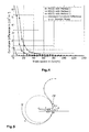
Display of the 2D curvilinear coordinate system to determine the track curvature,

Fig. 6

Curvature error distribution for different hypotheses,

Fig. 7

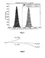
Test statistic for curvature determination method 3 for two different hypothesis: In dark grey the true curvature 10^-4 [m^-1] and in light grey the true curvature is 1/1749 [m^-1] which correspond to a minimum detectable curvature difference of MDCD=4.7176×10^-4 [m^-1] given a probability of wrong decision of P_wd =10^-5,

Fig. 8

Tracks configuration assumption,

Fig. 9

Minimum detectable curvature difference with respect to k₀ = 10^-4 [m^-1] obtained for the three different curvature determination methods κ₁, κ₂ and κ₃ vs. velocity are shown. For comparison, the standard German curvatures and their maximum allowed velocities are indicated by black lines. This plot is valid for a P _wd = 10^-5 and using consumer grade sensors,

Fig. 10

Minimum detectable curvature difference with respect to κ₀ = 10^-4 [m^-1] obtained with the three different curvature determination methods κ₁, κ₂ and κ₃ vs. velocity are shown. For comparison, the standard German curvatures and their maximum allowed velocities are indicated by black lines. This plot is valid for a P _wd = 10^-5 and using automotive grade sensors,

Fig. 11

Minimum detectable curvature difference with respect to κ₀ = 10^-4 [m^-1] obtained with the three different curvature determination methods κ₁, κ₂ and κ₃ vs. velocity are shown. For comparison, the standard German curvatures and their maximum allowed velocities are indicated by black lines. This plot is valid for a P _wd = 10^-5 and using tactical grade sensors,

Fig. 12

Availability degradation plot of curvature determination method κ₁ vs. velocity. for different IMU grades.

• The track curvature is determined by using the above described sensors in particular based on three different methods which will be described later in more detail.
• As it is shown for example in Fig. 10 each of these three curvature determination methods can result in a different minimum detectable curvature difference and a different vehicle speed dependency. For example, one method might result in lower required vehicle speeds which are necessary in order to be able to fulfill a required predefined wrong decision probability at different standard curvatures while another method might require higher speeds for the same preconditions. Since the performance order of the three methods is not constant over speed, it is preferred to switch between the three curvature determination methods depending on the speed and sensor quality. For example, if automotive grade sensors are used, it might be beneficial to use method 2 for 0-45km/h and method 3 for higher speeds (Figure 10). Thus, it is preferred to choose this curvature determination method for a first speed range which allows the vehicle to travel with lower speeds at given curvatures and wrong decision probabilities while a second (and possibly third) different curvature determination method is used for another speed range in which this other curvature determination method allows the vehicle to travel with lower speed in order to achieve the same results.
• It is possible to use a weighted combination of the different curvature determination methods, whereby the weight of each method depends on the velocity of the vehicle. This is due to the fact that with changing velocity the quality of each method may change as described above. In the example given above the weight of one method is 0 whereas the weight of the second (better) method is 1 at a first speed range and vice versa at the second speed range. In the now described alternative it is possible to adapt the weight for each method depending on the velocity of the vehicle.
• It is further possible to adapt the weight of each method depending on the camber of a track (namely the rotation around an x-axis running parallel to the longitudinal direction of the vehicle). It is further possible to choose the weight of each method based on an ascending or descending slope of the track (namely a rotation around the y-axis of the vehicle).
• By using the inventive method it is not only possible to determine standard curvatures. It is also possible to determine the reliability of the curvature determination for arbitrary curvatures.
• Fig. 1 shows qualitatively the expected error distribution p_k (k̃) of a curvature determination error. The curvature k̂ is defined as multiplicative inverse of the track radius, i.e., k̂=1/r. This error distribution is centered around the true curvature value k.
• The error distribution is used as an input for a threshold test, which for example can result in a minimum required curvature difference between two tracks. For this purpose a first threshold T₁ is defined in the first error distribution (see Fig. 2). A second threshold T₂ is defined in the second error distribution (see Fig. 3). Since in the example shown in Figs. 2 and 3 T₁=T₂, only one threshold T=T₁=T₂ is shown. The probability of false alert is marked with P_fa in Fig. 2. The probability of misdetection is marked with P_md in Fig. 3.Since both probabilities characterize the allowed decision error for either curvature one or two, they could be considered equal and can be called probability of wrong decision.
• The minimum curvature difference, which can be detected while fulfilling the required safety aspects (namely wrong decision probabilities), results from the difference between the two estimated curvature values MDCD = k̂ ₂ - k̂ ₁ (minimum detectable curvature difference). Fig. 4 shows some examples of these MDCD values, whereby three different curvature determination methods and inertial sensors of very high quality have been used. The curvature difference minima shown in Fig. 4 have been calculated based on a wrong decision probability of 10^-5 and tactical grade sensors. They are further dependent on the speed of the vehicle. The horizontal lines indicate the standard curvatures which are used in German railroad traffic (and their differences). The end of each of these horizontal lines indicates the maximum speed on these tracks. Therefore, the right, upper area shows vehicle speeds which are higher than the allowed German maximum speed on the respective track and hence, they are not relevant.
• The inventive method can also be applied for determining the position of the vehicle in a three dimensional space. In this case additional sensors will be necessary since a three dimensional position cannot be determined by using the described three sensors.
• Further in the inventive method a more complex error model can be used for example by assuming that the bias of the sensors is defective meaning that it is not constant over a time. The same applies to the scale factor of the sensors.
• The inventive method including more detailed algorithms will now be described in more detail.
First, a brief introduction is given:
• Global Navigation Satellite Systems (GNSS) are inspiring more and more safety of life applications like aviation, maritime and railway. However, for terrestrial applications in general and for rail applications especially, the signals provided by satellites are often blocked and reflected by surrounding obstacles like trees, terrain and buildings. So the signals coming to the receiving GNSS antenna might not be the direct signals but distorted ones. This has a huge impact on the achievable position accuracy, system availability, continuity and integrity. Consequently, pure satellite based navigation/localization systems may fail to provide the required system performance particularly for safety-of-life critical railway applications. Furthermore, GNSS is generally delivering an absolute positioning which is often not what matters in rail navigation. Here, trains can only move on well-defined smooth tracks and the localization objective consists of determining on which track segment and at which level in this segment the train is located and in which direction it moves. This information is crucial for collision avoidance system such as RCAS¹. In case the position of the trains within the track map is reliably and continuously known, possible train collision situations can be identified and avoided on time.
  ¹Railway Collision Avoidance System (RCAS) - a project of the German Aerospace Center (DLR) - investigating, developing and validating a 'safety overlay' system which can be deployed on top of any existing safety infrastructure in train networks. The core idea of RCAS is to broadcast the position and intended track of trains as well as additional information like vehicle size to all other trains in the area using an ad-hoc train-to-train communication system. This enables train drivers to have an up-to-date accurate knowledge of the traffic situation in the vicinity, and act in consequence.
• There are different approaches to solve this localization problem: The two main methods are map matching and dead reckoning system. The former obtains an absolute 3D position estimating using GNSS and additional sensors for each epoch and matches this position with the track map. This could be done by choosing the closest point in the track as the best estimate. In the second approach, the movement of the train relatively to a reference point is estimated incorporating all available sensors. Hence the position within the map is directly known. This approach can provide a more accurate and reliable solution since no intermediate solution is computed. Train localization/navigation using GNSS and IMU has been investigated by many different authors some of them providing novel and promising techniques using Bayesian filters [6].
• One of the most critical situations for dead reckoning systems are switches. Here, the train localization system needs to detect reliably and automatically with low latency which track was taken by the train. This decision can be done by determining the curvature of the track. In [1], low-cost MEMS gyroscopes are used for curvature detection. By applying a matched filter, the detection is optimized for real-time operations. However, the reliability of the detection cannot be determined which is mandatory for integrity assessment.
• In this paper, we define and investigate the usage of three different test statistics to classify the curvature of the track instantaneously. We also address the performance of this classification with respect the false alert and miss-detection probabilities. Based on these results, we determine the minimum velocity which is necessary to reliably identify the curvature. In our approach, we use three inertial sensor components, i.e., an along-track and a cross-track accelerometer and a heading rate gyroscope. As a matter of course, the classification performance depends strongly on the quality of the sensor. Hence, we discuss the sensor error model, derive the corresponding stochastic differential equation and the Gaussian overbound of the stochastic process solution. We then outline and analyze the three possible curvature computation methods expressed as ratios of sensor outputs. Later the resulting test statistics of these three methods are evaluated with respect to standard German track curvatures. Finally, we conclude this paper with a summary and a direction for future work.
I. SYSTEM MODEL A. General System Assumption
• In this paragraph we list the major assumptions that we make except those related to the error model extensively discussed in the following section.
• We neglect the effect of the gravity related errors in the inertial sensors. That is we assume that the plan of motion (formed by the along track and cross track vectors) is perpendicular to the gravity vector. Hence, the acceleration due to the gravity is not measured by the along and cross track sensors. This assumption might be valid due to the planar construction requirement of switches in general.
• We assume that the accelerometers are perfectly aligned with the body frame of the train. Hence, no along track and cross track misalignment are considered.
• For the heading rate gyroscope, we further assume a perfectly alignment of the motion plan. We further assume a perfect correction of the turn rate errors due to the Coriolis force and the earth rotation.
B. Inertial Sensor Error Model
• Inertial error models have been widely discussed in the literature. According to [2], however it is sufficient to use a simplified version of sensor model. Assuming the misalignment of the different sensors with respect to the reference axes are known, the measured sensor output can be written as: $$\hat{m}\left(t\right)=\left(1+s_f\right)m\left(t\right)+b\left(t\right),$$

  

  
  where m̂(t) is the measured sensor output such as angular turn rate and a 1-D acceleration, respectively. The true value of this quantity is denoted as m(t) and can be used as the input value in the simulations. It is possible to simulate different type of scenarios as for example vibrations or constant acceleration, deceleration [5]. An ideal accelerometer would directly sense m(t) but in a non ideal case, the measured acceleration or turn rate is decomposed into a proportional part (proportional to a scaling factor s_f ) and a time dependent drift part b(t). The latter can be modeled by a constant offset b ₀ as well as a time varying b ₁(t) and a sampling noise component η _m : $$b\left(t\right)={\mathrm{<figure-callout\; id="0"\; label="b"\; filenames="imgf0002.png,imgf0005.png"\; state="\{\{state\}\}">b</figure-callout>}}_0+b_1\left(t\right)+{\eta }_m\mathrm{.}$$

  
• We assume that the offset b ₀ stays constant during each run and is corrected by an initial calibration of the sensors. Additionally, the sampling noise is assumed to be Gaussian distributed with zero-mean and a variance ${\sigma }_m^{}$ ${}_2^{}\mathrm{.}$

  

  The time-varying component is represented by a 1st-order Gauss-Markov process which can be expressed mathematically by $${\dot{b}}_1\left(t\right)=-\frac{1}{\tau }{b}_1\left(t\right)+{\eta }_b,$$

  

  
  where τ is the correlation time and η _b is the driving noise which can be assumed to be Gaussian distributed with zero mean and variance ${\sigma }_b^{}$ ${}_2^{}\mathrm{.}$

  

  This is also known as an Ornstein-Uhlenbeck process with a rate of mean reversion of $\frac{1}{\tau }$

  

  and a volatility σ_b .
• In order to obtain realistic values for the sampling and driving noise component as well as for the time correlation, real sensor measurements have to be analyzed with the help of the Allan variance and auto-correlation function of a long series of zero-input measurements [2]. Exemplary, we show the resulting parameters of three different qualities of inertial sensors in Table 2. We will use these parameters and values throughout our paper.
C. Stochastic Differential Equation and its Solution
• Due to the focus of this paper, we need to investigate not only the error of the measurement itself but also its propagation via integration. In the following, we look into the stochastic differential equation issues to solve our problem.
• Let us first consider a one dimensional translational acceleration (without attitude change) only. The position of the rover can be determined using only one accelerometer or the combination of redundant accelerometers in the direction of the acceleration. We combine the Equation (1) and (2) and obtain: $$\hat{m}\left(t\right)=\left(1+s_f\right)m\left(t\right)+{\mathrm{<figure-callout\; id="0"\; label="b"\; filenames="imgf0002.png,imgf0005.png"\; state="\{\{state\}\}">b</figure-callout>}}_0+b_1\left(t\right)+{\eta }_m,$$

  

  
  Let the error of the measurement be noted by Δm̂(t) with: $$\begin{array}{ll}\mathrm{\Delta }\hat{m}\left(t\right)& =\hat{m}\left(t\right)-m\left(t\right)\\ & =s_{f}m\left(t\right)+{\mathrm{<figure-callout\; id="0"\; label="b"\; filenames="imgf0002.png,imgf0005.png"\; state="\{\{state\}\}">b</figure-callout>}}_0+b_1\left(t\right)+{\eta }_m\mathrm{.}\end{array}$$

  
• The time-varying bias b ₁(t) is the solution of the stochastic differential Equation (3). If we rewrite this equation into the Ito-form and introduce a one-dimensional Brownian motion B_t, we obtain for the sensor time-varying bias the following [9]: $$d{b}_1\left(t\right)=-\frac{1}{\tau }{b}_1\left(t\right)\mathit{dt}+{\sigma }_{b}d{B}_{t,1}\mathrm{.}$$

  
• The corresponding error u(t) introduced by the integration of the measurement error can be expressed by: $$\mathit{du}\left(t\right)=\left(s_{f}m\left(t\right)+{\mathrm{<figure-callout\; id="0"\; label="b"\; filenames="imgf0002.png,imgf0005.png"\; state="\{\{state\}\}">b</figure-callout>}}_0+b_1\left(t\right)\right)\mathit{dt}+{\sigma }_{m}d{B}_{t,2}$$

  
• These equations can be applied to all our measurements required for our test statistics, i.e., to the cross track and along track accelerometer as well as to the heading rate gyroscope.
• In order to solve our problem, let us define a state vector x(t) = (b ₁ (t) u(t)) ^T . By applying the previous defined equations, we can rewrite our problem as follows: $$d\mathit{x}\left(t\right)=\left(\begin{array}{c}d{b}_1\left(t\right)\\ \mathit{du}\left(t\right)\end{array}\right)={\mathit{\beta }}_t\left(\mathit{x}\left(t\right)\right)\mathit{dt}+\mathit{S}d{\mathit{b}}_t,$$

  

  $$\begin{array}{c}{\mathit{\beta }}_t=\left(\mathit{x}\left(t\right)\right)=\left(\left(\begin{array}{c}-1/\tau \\ 1\end{array}\right)b_1\left(t\right)+\left(\begin{array}{c}0\\ s_{f}m\left(t\right)+{\mathrm{<figure-callout\; id="0"\; label="b"\; filenames="imgf0002.png,imgf0005.png"\; state="\{\{state\}\}">b</figure-callout>}}_0\end{array}\right)\right),\\ \mathit{S}=\left(\begin{array}{cc}{\mathrm{<figure-callout\; id="0"\; label="\sigma \; b"\; filenames="imgf0002.png,imgf0005.png"\; state="\{\{state\}\}">\sigma </figure-callout>}}_b& 0\\ 0& {\sigma }_m\end{array}\right)\mathrm{and}d{\mathit{b}}_t={\left(\begin{array}{cc}d{B}_{t,1}& d{B}_{t,2}\end{array}\right)}^T\mathrm{.}\end{array}$$

  
• In general, two different approaches are used to solve these kind of problems. The first one uses a generator of the Ito-diffusion process defined by the stochastic differential equation and derive a partial differential equation, so called Kolmogorov Forward Equation or Fokker Planck Equation. Its solution is a transition probability density function of the solution process (see [4] and [3]).
• The second method takes advantage of the fact that the process solution is Gaussian distributed, if the initial state densities can be assumed to be also Gaussian distributed. Hence, it is sufficient to investigate the evolution of the corresponding expectation and variance of the transition density function. In the section below, we apply the second concept and discuss the results.
D. Analytical Form of the Transition Density solution of the Stochastic Differential Equation
• We consider a state vector comprising the drift of the sensor and the integral with respect to time of the sensor error (e.g., the velocity error for an accelerometer or the heading error for an angle rate gyro). So we need to solve this problem: $$\mathit{x}\left(t\right)=\mathit{x}\left(0\right)+{\int }_0^t{\mathit{\beta }}_l\left(\mathit{x}\left(l\right)\right)\mathit{dl}+\mathit{S}d{\mathit{b}}_t,$$

  

  
  where x(0) = (b ₁(0) u(0)) ^T is our initial state vector. Recall from before that this can be considered as an Ornstein-Uhlenbeck process in case of a continuous time problem or as an 1st-order auto-regressive process with equilibrium at 0 in case of a discrete time problem. Thus, we can reformulate Equation (6) as integrated process: $$b_1\left(t\right)={\mathrm{<figure-callout\; id="1"\; label="b"\; filenames="imgf0002.png,imgf0004.png"\; state="\{\{state\}\}">b</figure-callout>}}_1\left(0\right)e^{-\frac{t}{\tau }}+{\sigma }_b{\int }_0^t{e}^{\frac{l-t}{\tau }}d{B}_{l,1}\mathrm{.}$$

  
• Under the assumption that the initial value of the time-variant bias b ₁(0) can be considered as normal distributed random variable with mean

  

  and variance

  

  the solution of the bias differential equation results also in a Gaussian distributed quantity, where the corresponding mean and variances are given by:

  
• Similar steps, we can apply to the full stochastic differential equation x(t) = (b ₁(t) u(t)) ^T and we obtain: $$\mathit{x}\left(t\right)=\left(\begin{array}{cc}{e}^{-t/\mathrm{<figure-callout\; id="0"\; label="\tau "\; filenames="imgf0002.png,imgf0005.png"\; state="\{\{state\}\}">\tau </figure-callout>}}& 0\\ 0& 1\end{array}\right)\mathit{x}\left(0\right)+\mathit{h}\left(t\right)+\left(\begin{array}{c}0\\ {\sigma }_m{B}_{t,2}\end{array}\right),$$

  

  
  where $\mathit{h}\left(t\right)=\left(\begin{array}{c}{\sigma }_b{\int }_0^t{e}^{\frac{l-t}{\tau }}d{B}_{l,1}\\ {\int }_0^t\left(s_{f}m\left(l\right)+{\mathrm{<figure-callout\; id="0"\; label="b"\; filenames="imgf0002.png,imgf0005.png"\; state="\{\{state\}\}">b</figure-callout>}}_0+b_1\left(l\right)\right)\mathit{dl}\end{array}\right)\mathrm{.}$

  

  To solve our problem, we propose to compute the expectation and variance of the process in a snapshot manner, i.e., for each time step. So, for the expectation we have to solve:

  

  since

  

  by definition of a Brownian motion. The two components of the sum can be rewritten as:

  
• The derivation of the corresponding state vector covariance matrix is quite complex, so we just want to state the result here in this paper.

  
• Please note that the covariance matrix is symmetric, i.e., c ₁₂(t) = c ₂₁(t). Also we define an auxiliary Gaussian random variable ${\epsilon }_{\tau }\left(t\right)={\int }_0^t{\int }_0^r{e}^{\frac{l-r}{\tau }}d{B}_{l,1}\mathit{dr}\mathrm{.}$

  

  So, we get

  
• Recall that ε_τ (t) is function of B _t,1, we kept the cross products as non necessarily zero terms. In fact (See Appendix A for more details), the mean

  

  and the variance of ε_τ (t) is given by ${\sigma }_{{\epsilon }_{\tau }\left(\mathrm{<figure-callout\; id="2"\; label="t"\; filenames="imgf0005.png,imgf0006.png"\; state="\{\{state\}\}">t</figure-callout>}\right)}^2=t{\tau }^2-\frac{3}{2}{\mathrm{<figure-callout\; id="3"\; label="\tau "\; filenames="imgf0002.png,imgf0005.png"\; state="\{\{state\}\}">\tau </figure-callout>}}^3+2\frac{{\tau }^3}{e^{\frac{t}{\tau }}}-\frac{{\mathrm{<figure-callout\; id="3"\; label="\tau "\; filenames="imgf0002.png,imgf0005.png"\; state="\{\{state\}\}">\tau </figure-callout>}}^3}{2{\mathrm{<figure-callout\; id="2"\; label="e"\; filenames="imgf0005.png,imgf0006.png"\; state="\{\{state\}\}">e</figure-callout>}}^{2\frac{t}{\tau }}}$

  
• Finally we observe that the covariance matrix

  

  is not diagonal in the general case.
• We observe that when the random variables in the model of the sensor are all Gaussian distributed (including the initial point b ₁(0) and u0, the state vector is also Gaussian distributed. Therefore the propagation of the mean and the variance is sufficient if we want to characterize the whole distribution.
• Given all these expressions, we can deduce the expectation and the variance of the state vector as function of time t, time constant τ and the parameters of the problem.

  
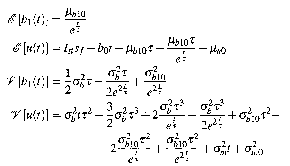
• By using Equation (5), we deduce the expectation and the variance of the sensor error:

  
II. SNAPSHOT TRACK CURVATURE CLASSIFICATION A. Curvature Determination
• In the following section, the physical assessment of the track curvature is introduced and three different methods are outlined. Let s(t) being the curvilinear abscissa representing the length of the arc represented by the track from a reference position to a current point. The velocity vector of the train is v = ṡe _AT and the acceleration vector is: $$\mathbf{a}=\frac{d\mathbf{v}}{dt}=\frac{d\left(\dot{s}{\mathbf{e}}_{\mathit{AT}}\right)}{dt}=\ddot{s}{\mathbf{e}}_{\mathit{AT}}+\dot{s}{\dot{\mathbf{e}}}_{\mathit{AT}}$$

  
• In this expression and in the rest of this chapter we drop the time t for simplification. The dot above variables always means the derivative of the given variable with respect to time. To express ė _AT , we use the notations of Figure 5. During dt, the point M moved from s to s+ds and the unit along track vector has rotated with the angle dψ. This drives to the following relation: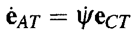 $${\dot{\mathbf{e}}}_{\mathit{AT}}=\dot{\psi }{\mathbf{e}}_{\mathit{CT}}$$

  
• Observing that the acceleration vector lies in the osculating plan defined by (e _AT, e _CT ), we can decompose the acceleration into 2 components: and taking the same notation as for the unit vectors, we have: $$\mathbf{a}\left(t\right)=a_{\mathit{AT}}{\mathbf{e}}_{\mathit{AT}}+a_{\mathit{CT}}{\mathbf{e}}_{\mathit{CT}}$$

  

  $$a_{\mathit{AT}}=\ddot{s}$$

  

  $$a_{\mathit{CT}}=\dot{s}\dot{\psi }$$

  
• We observe that ṡ = rψ̇, so we have the following expression: $$a_{\mathit{CT}}=r{\dot{\psi }}^2$$

  
• With r being the local radius of the trajectory.
• We observe that Equation (11) can be expressed in terms of ṡ rather than ψ̇ and observing that ||v|| = ṡ, we have: $$a_{\mathit{CT}}=\frac{{\Vert \mathbf{v}\Vert }^2}{r}$$

  
• There is a relation between the speed of the train, the cross track acceleration and the heading rate for a given trajectory.
• We have the following relations: $$a_{\mathit{CT}}=r{\dot{\psi }}^2=\frac{{\Vert \mathbf{v}\Vert }^2}{r}$$

  
• In this equation, we can directly sense the cross track acceleration a_CT, the heading rate ψ̇ and indirectly the velocity of the train v (integral of the along track acceleration). This is an important a-priori information that can be used in a test statistic to decide which direction the train has taken after a switch. By convention we will choose to work with the curvature rather than with r. Let κ = 1/r the relation above can be written as follows: $$a_{\mathit{CT}}=\frac{{\dot{\psi }}^2}{\kappa }=\kappa {\Vert \mathbf{v}\Vert }^2$$

  
• In this equation, κ can be obtained in three different ways: $${\kappa }_1=\frac{{\dot{\psi }}^2}{a_{\mathit{<figure-callout\; id="2"\; label="CT\; \kappa "\; filenames="imgf0005.png,imgf0006.png"\; state="\{\{state\}\}">CT</figure-callout>}}}$$

  

  $${\kappa }_{}$$ $${}_2=\frac{\left|\dot{\psi }\right|}{\Vert \mathbf{v}\Vert }$$

  

  $${\kappa }_3=\frac{a_{\mathit{CT}}}{{\Vert \mathbf{v}\Vert }^2}$$

  
• All three methods can also be used in a non-stationary scenario, i.e., while the train is moving. Otherwise the curvature determination might be not defined. That is if a_CT = 0, κ₁ is undefined and if ||v(t)|| = 0, κ₂ and κ₃ are undefined.
B. Test Statistic
• In this section, we analyze the resulting test statistic based on the three curvature determination methods. To compute κ_i, i = 1, ... , 3, we need the heading rate, along-track and cross-track accelerations. These measurements are distorted by sensor errors which can be modeled as described in Section I-B. Using the SDE results from Section I-C, we can access the error distribution of each measurement required to determine the curvature. However, the distribution of curvatures itself is not simple to derive since we have to obtain the distribution of a ration of random variables. The resulting distribution might not be symmetric and can be even heavy tailed. In the following, we discuss the expected behavior of the test statistics.
• Naturally, if all measurements would be error-free, all three curvature computations would deliver the same result κ₁ = κ₂ = κ₃. But due to the randomness of the measurements of a_CT (t), ψ̇ (t) and v(t), the performance of the obtained curvatures can only be characterized in terms of distribution.
• First method κ₁: The measurements of this methods can be directly sensed, so no integration of the measurements is required. However, we can see that if the curvature of the path is zero, i.e., the track is straight, the numerator will take positive random values following a χ ² distribution and the denominator will take values centered at 0. This induces fat tails in the distribution of κ₁. Consequently, it might be not very promising to use this method for the hypothesis test.
• Second method κ₂: Here, we observe a ratio between a normally distributed random variable and a folded normal distribution (the absolute value of a normally distributed random variable). In the case of a ratio between two independent, normally distributed random variables with zero mean, the distribution of the ratio follows a Cauchy distribution. In the case of non-centered distributions, it has been demonstrated [7] that the probability density function can be written as follows: $$\begin{array}{c}{\mathrm{<figure-callout\; id="2"\; label="p\; K"\; filenames="imgf0005.png,imgf0006.png"\; state="\{\{state\}\}">p</figure-callout>}}_{K_{}^{}}\left({\mathrm{<figure-callout\; id="2"\; label="\kappa "\; filenames="imgf0005.png,imgf0006.png"\; state="\{\{state\}\}">\kappa </figure-callout>}}_2^{*}\right)=\frac{\alpha \exp \left\{\frac{1}{2}\frac{{\mathrm{<figure-callout\; id="2"\; label="\alpha "\; filenames="imgf0005.png,imgf0006.png"\; state="\{\{state\}\}">\alpha </figure-callout>}}^2}{\gamma }-\frac{1}{2}\mathrm{<figure-callout\; id="3"\; label="\xi \; \gamma "\; filenames="imgf0002.png,imgf0005.png"\; state="\{\{state\}\}">\xi </figure-callout>}\right\}}{{\gamma }^{}}\frac{1}{\psi }\times \left(2\mathrm{\Phi }\frac{\alpha }{\gamma }-1\right)+\\ +\frac{1}{\mathit{\gamma \pi \psi }}\exp \left\{-\frac{1}{2}\xi \right\},\end{array}$$

  

  
  where

  

  and ${\mathrm{<figure-callout\; id="2"\; label="\kappa "\; filenames="imgf0005.png,imgf0006.png"\; state="\{\{state\}\}">\kappa </figure-callout>}}_2^{*}=\frac{\dot{\psi }\left(t\right)}{\mathbf{v}\left(t\right)},$

  

  and $\mathrm{\Phi }\left(u\right)={\int }_{-\infty }^u\frac{1}{\sqrt{2\pi }}\exp \left\{-\frac{1}{2}{\mathrm{<figure-callout\; id="2"\; label="z"\; filenames="imgf0005.png,imgf0006.png"\; state="\{\{state\}\}">z</figure-callout>}}^2\right\}\mathit{dz}\mathrm{.}$

  

  This expression is not representing the test statistic of interest κ₂ for which no closed form could be found.
• Third method κ₃: Similar to κ₂, to nominator can be seen as normal distributed random variable. However, the denominator is not only linear dependent on an folded normal distributed random variable, but quadratically dependent. Also in this case no close for solution can be found.
• In the remaining paper, we assess the distributions of κ _i, i = 1,...,3 via Monte-Carlo simulations. As derived before we can compute the probability distributions of a_CT (t), ψ̇(t) and v(t) depending on the quality of the sensor as well as initialization. Please note that the direct use of heavy tailed distributions can generate instabilities of the test statistics. In this case, the mean and variance may not exist especially in the case of high densities around zero for the test statistics denominators.
• One possibility is to exclude the samples of a_CT (t), ||v(t)|| and ||v(t)||² that are close to zero, or in an interval around zero. The area to exclude using a pretest should not be too large for one reason essentially: the exclusion reduces the availability of the test statistics (for each sample falling in the excluded area, the corresponding test statistics is set as unavailable). But the closer the exclusion bounds are to zero, the wider the distribution of the test statistics and therefore the smaller the minimum detectable curvature difference (MDCD).
C. Hypothesis Test
• To classify or identify a certain curvature, we compare our computed curvature with a threshold. The latter, we have determined by a standard hypothesis test algorithm. In the following, this algorithm is described briefly.
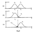
• First of all, reliable knowledge of curvature determination error behavior is required. We denoted this curvature error probability density function as p_K (κ). We assume that this pdf is centered at the true curvature. Then we can define the distributions for two different track curvature hypotheses that we want to test. For example, after a switch a train might have two possibilities to move on, i.e., track segment one with curvature κ _a or track segment two with curvature κ _b . Figure6 (a) illustrates the resulting curvature pdfs, if either track segment one p_K (κ|H_a ) or track segment two p_K (κ|H_b ) has been taken. In order to make a decision, we have to define a threshold T against which we compare our curvature measurements. If our measurement is below the obtained threshold, we decide for H_a and if it exceeds this threshold, we decide for H_b. To find this threshold we have to consider the probability of false alarm P _fa. This probability is a system reliability requirement and accounts for the case, where we decided for H_b (indicated segment two, while hypothesis H_a was correct (the train took the segment one). This is depicted on Figure 6 (b)). Consequently, the threshold is given by $$T=\arg \left(P_{\mathrm{fa}}=P_K\left(\kappa >T|H_a\right)={\int }_T^{\infty }{p}_K\left(\kappa |H_a\right)\mathit{d\kappa }\right)\mathrm{.}$$

  
• Similar considerations can now be done for hypothesis H_b as well. A probability of missed detection, i.e., we decided for segment one while the train took segment two, is normally defined as $$P_{\mathrm{md}}=P_K\left(\kappa <T|H_b\right)={\int }_{-\infty }^T{p}_K\left(\kappa |H_b\right)\mathit{d\kappa }\mathrm{.}$$

  
• This is displayed in Figure 6 (c). P _md is also a system reliability requirement and normally pre-defined by the system. So for a given P _md, we can find a κ _m such that $${\kappa }_m=\arg \left({\int }_{-\infty }^T{p}_K\left(\kappa |H_m\right)\mathit{d\kappa }=P_{\mathrm{md}}\right),$$

  

  
  where H_m is the hypothesis that the train has taken a track with curvature κ _m . Thus, we can define a minimum detectable curvature difference MDCD = κ _m - κ _a for the given system requirements of false alert and missed detection. Both probabilities, P _md and P _fa indicate that a wrong decision is made. Since we want to protected hypothesis H_a and H_b equally, we set P _fa = P _md = P _wd, where wd stands for wrong decision.
• In Figure (7), we show two histograms observed while using the test statistics of κ₃. The train moves with a speed of 50 [km/h] and the coasting time is 75 seconds. By coasting time we understand the time for which the inertial sensors run free, so the time after initialization.
• We assume that during the coasting period, the speed is obtained by integrating the along track acceleration. In dark gray, we show the distribution of the test statistic under the hypothesis H_a (with a curvature radius of 10 km) and the light gray curve corresponds to the hypothesis H_b (with a curvature radius of 1749 m). So the minimum detectable curvature difference is equivalent to MDCD = 1/1749 - 10^-4 = 4.7176 × 10^-04 [m^-1]. The probability of wrong detection is set to P _wd = 10^-5 and is generally a requirement based on the level of hazard for being on another track than the one expected. This risk is usually defined as a probability of being in this hazardous situation during a predefined exposure time.
III. SIMULATION AND EVALUATION A. Simulation Environment
• For simulation, we used standard curvatures found in the German railway. A summary of available curvatures and corresponding maximum allowed train velocity can be found in Table 1. As mentioned before, the error model parameters of the used inertial sensors are shown in Table 2. Table 1: Basic Design Parameters of German standard switches [8]

  radius r in m	curvature c in 10-3 1/m	max velocity ν max in km/h
  190	5.26	40
  300	3.33	50
  500	2.0	60
  760	1.32	80
  1200	0.83	100
  2500	0.4	120

• We propose to investigate a curvature detector based on the three test statistics defined in Equations (15, 16, 17). The path identification after a switch is crucial for train surveillance and train collision avoidance systems. If we assume not to know the itinerary but just the map with the switch locations and the curvature of the possible paths after the switches, it is possible to determine the path followed by the train with a confidence depending on the quality of the sensors.
• In the simulations, we use a sensor having the following characteristics:
• We solve the stochastic differential system for the expectation and the variance for all three different sensor grades.
• We draw paths following the process distributions calculated and we build the histograms for each test statistic κ₁, κ₂ and κ₃.
• The initial along track velocity uncertainty might be given by GNSS and is assumed to have a σ _ν̂(0)0 = 0.05 [m/s]. When GNSS is not longer available, the velocity is drifting from its initial value considering a coasting using along track accelerometer.

  
B. Assumptions for train localization
• At a given initial epoch we assume to know the position and the direction of displacement of the train (for example at the departure station). The localization problem consists of determining the track segment ID, the direction of displacement and the curvilinear abscissa on the track segment.
• A track segment is defined as a path between two switches. We assume that between two guaranteed positions (e.g., obtained by GNSS and verified by a receiver autonomous integrity monitoring), velocity fixes a coasting with the inertial unit based on along track, cross track accelerometers and a heading rate gyro using the characteristics defined in Table 2. The coasting time is not longer than 1 second when at least 5 satellites are visible which is generally the case. But in some cases (long tunnels or in the general case of bad satellite visibility or when the satellite signals are blocked or reflected by a strong multipath environment) the coasting time could be last much longer (up to several minutes). Nevertheless, as long as the information used is not integrated in the time to obtain velocity, position or heading angle, the error in the information is stationary and can be overbounded by a Gaussian distribution for a non zero required integrity risk. This overbound remains constant assuming the error is a stationary process.
• In Figure (8) we show the topology we adopt for the switch scenario. We assume at each switch, only two possible tracks can be taken.
C. Minimum Detectable Curvature Difference
• We have seen in the precedent section that the probability of wrong decision is an important system reliability requirement. The question we need to answer is now: What is the minimum curvature difference for which we can detect an alternative curvature with a probability of 1 - P _WD? In order to answer this question, we first have to determine our test statistic threshold T = fct(κ₀, P _WD) which is a function of the curvature of our H_a hypothesis κ₀ and the allowed probability of false alert. Then we generate the probability density function for a continuously growing curvature κ _m > κ₀ until we get: $$\underset{-\infty }{\overset{T}{\int }}{p}_K\left({\kappa }_i|H_m\right){\mathit{d\kappa }}_i=P\left({\kappa }_i<T|H_m\right),$$

  

  
  where H_m is the hypothesis centered at κ _m and κ _i , for i = 1,... 3 are the different test statistics defined in Equation (15, 16,17). Finally, the MDCD is κ _m - κ₀.
• The MDCD is a function of the velocity of the train. Intuitively the larger the velocity of the train, the smaller the dispersion of the test statistic.
• We investigate the MDCD for each test statistic as function of the train velocity at a switch and for different IMU qualities. In the following investigations, we set our curvature of hypothesis H_a to κ₀ = 10^-4 [m^-1].
• In Figures (9, 10, 11) we have plotted the corresponding MDCD vs. the velocity for each test statistic and for each IMU quality. The black horizontal lines represent the standard curvatures of tracks observed in Germany. Each standard line starts at ν = 0 [km/h] and stop at the maximal allowed velocity for the corresponding curvature. The larger the curvature, the smaller the maximal allowable speed. The initial and reference curvature to be almost zero (a curvature of exactly 0 lends to a singularity). We see that the lower the velocity, the higher the MDCD.
• Although κ₁ seems to provide acceptable performance in the case of tactical grade IMU, its low availability for a large range of velocities see Figure (12) makes it unusable for the simulated scenario. Only κ₂ and κ₃ are providing acceptable results (their availabilities were always 100% for any type of IMU).
• For tactical grade IMU, we see a very effective κ₂ based test statistic. In fact the combination of high accurate velocity and high performance heading gyro provides a sharp distribution and therefore a clear signature when the train change its track. For this tactical grade IMU, κ ₂ and κ ₃ are not crossing in the velocity range [0 - 200] [km/h].
• For both the consumer and the automotive grade IMUs, the MDCD curves cross at a speed of approximately 50 [km/h]. This suggests a velocity based test selection: below 50 [km/h] we use κ ₂ to make our decision and above this limit, we use κ₃ which performs better. A more efficient strategy could consist of defining a weighted combination of both test statistics enabling even lower MDCD. However, this is beyond the scope of this paper.
• The results obtained suggest a weighted sum of κ₂ and κ₃ in order to improve the detectability. Some intrinsic problems may appear because of the dependency of all 3 test statistics. Correlations need to be considered while seeking an optimal combination of curvature types.
IV. CONCLUSION
• In this paper we explored three different ways to determine track curvatures. The tests are based on ratios of random variables that can be directly sensed like the heading rate gyro and the cross track acceleration and indirectly sensed like the speed of the train which can be obtained by an integration of the along track acceleration.
• The expectation and the variance of the Gaussian overbound of the sensor errors are analytically expressed and the test statistics after pretreatment of the random denominators (exclusion of an interval around zero to prevent heavy tailed distributions) are investigated using Monte Carlo simulations. The minimum detectable curvatures difference is determined for three different classes of IMUs, namely consumer, automotive and tactical grade. The resulting MDCD curves have been compared to standard curvatures and their performance have been assessed.
• It is shown that κ₁ in addition to being unavailable a large part of the time (exclusion of the high density around zero of the cross track acceleration) provides when a bad performance. In comparison, κ₂ and κ₃ show best results with a maximum availability when the train is moving. A performance crossover can be observed for the consumer and automotive grade IMUs. That is κ₃ can outperform κ₂ when the velocity of the train is larger than 50 km/h. However, κ₃ depends on the cross track acceleration which is difficult to sense in a more realistic dynamic scenarios (for a non-perfect horizontal plan of motion, for which the gravity vector may introduce a component in cross track direction). In contrast, κ₂ shows a real improvement as it can be reliably used for a large range of velocities. Furthermore, it has a dependency on the heading rate rather than on the accelerations which makes it more robust to realistic scenarios (non-perfect horizontal displacements).
• Future studies will consider a generalization of this concept for a three dimensional tracks (with gravity vector not always perpendicular to the motion plan), misalignment of sensors, transition curvatures. The performance crossover observed for κ₂ and κ₃ for low cost IMUs suggests to use a combination of both test statistics which is investigated in a future paper. Another investigation might consider the minimum probability of wrong detection for a given type of IMU and as function of the speed at the switch. This approach can give the level of safety achieved by different types of IMU.
APPENDIX A EXPECTATION AND VARIANCE OF BROWNIAN MOTIONS (APPEARING IN THE ANALYTICAL FORM OF THE EXPECTATION AND THE VARIANCE OF THE ALONG TRACK VELOCITY ERROR) A. Expectation of the Brownian Motion
• Consider the following Brownian Motion: $\mathit{x}\left(t\right)=B_t{\int }_0^t{B}_s\mathit{ds},$

  

  so we can express its expected value as

  
• We define Δt = t/n and t_k = kΔt. The Riemann sum approximation of x(t)is: $$X_{t_n}=B_{t_n}{\displaystyle \sum _{k=0}^{n-1}}{B}_{t_k}\mathrm{\Delta }t$$

  

  

  

  

  where t_n Λ t_k = min (t_n, t_k )

  

  

  

  
• By continuity we have

  

  when n → ∞ and

  
• B. Expectation of $\mathit{x}\left(t\right)={\mathit{\eta }}_t\left(\tau \right){\int }_0^t{e}^{\frac{l-t}{\tau }}d{\mathrm{<figure-callout\; id="1"\; label="B\; b"\; filenames="imgf0002.png,imgf0004.png"\; state="\{\{state\}\}">B</figure-callout>}}_{b_{}}$

  

  $${\eta }_t\left(\tau \right)={\int }_0^t{B}_r\mathit{dr}-\frac{1}{\tau }{\int }_0^t{\int }_0^r{e}^{\frac{l-r}{\tau }}{B}_u\mathit{dldr}\mathrm{and}{\int }_0^t{e}^{\frac{l-r}{\tau }}d{\mathrm{<figure-callout\; id="1"\; label="B\; b"\; filenames="imgf0002.png,imgf0004.png"\; state="\{\{state\}\}">B</figure-callout>}}_{b_{}}={\mathit{<figure-callout\; id="1"\; label="B\; b"\; filenames="imgf0002.png,imgf0004.png"\; state="\{\{state\}\}">B</figure-callout>}}_{b_{}}-\frac{1}{\tau }{\int }_0^t{e}^{\frac{l-t}{\tau }}{\mathrm{<figure-callout\; id="1"\; label="B\; b"\; filenames="imgf0002.png,imgf0004.png"\; state="\{\{state\}\}">B</figure-callout>}}_{b_{}}\mathit{dl}\mathrm{.}$$

  

  $$\begin{array}{r}\mathit{x}\left(t\right)={\int }_0^t{B}_t{B}_r\mathit{dr}-\frac{1}{\tau }{\int }_0^t{\int }_0^r{e}^{\frac{l-r}{\tau }}{B}_t{B}_u\mathit{dldr}-\\ -\frac{1}{\tau }{\int }_0^t{e}^{\frac{r-t}{\tau }}{B}_r\mathit{dr}{\int }_0^t{B}_r\mathit{dr}+\\ +\frac{1}{{\mathrm{<figure-callout\; id="2"\; label="\tau "\; filenames="imgf0005.png,imgf0006.png"\; state="\{\{state\}\}">\tau </figure-callout>}}^2}{\int }_0^t{e}^{\frac{r-t}{\tau }}{B}_r\mathit{dr}{\int }_0^t{\int }_0^r{e}^{\frac{l-r}{\tau }}{B}_u\mathit{dldr}\end{array}$$

  

  
• Finally we have:

  
C. Variance of η_t (τ)
• We recall that ${\eta }_t\left(\tau \right)={\int }_0^t{B}_r\mathit{dr}-\frac{1}{\tau }{\int }_0^t{\int }_0^r{e}^{\frac{l-r}{\tau }}{B}_u\mathit{dldr}$

  
• The expectation of γ_t (τ) is equal to zero. Therefore the variance is:

  

  

  

  
REFERENCES
1. [1] Antoni Broquetas, Adolf Comerón, Antoni Gelonch, Josep M. Fuertes, J. Antonio Castro, Damià Felip, Miguel A. López, and José A. Pulido. Track Detection in Railway Sidings Based on MEMS Gyroscope Sensors. Sensors, 12(12):16228-16249, 2012.
2. [2] Demoz Gebre-Egziabher. Design and Performance Analysis of a Low-Cost Aided Dead Reckoning Navigator. PhD thesis, Stanford University, 2004.
3. [3] Anja Grosch and Boubeker Belabbas. Parameter Study of Loosely Coupled INS/GNSS Integrity Performance. In Proceedings of IEEE/ION PLANS, Myrtle Beach, SC, USA, 24-26 Apr 2012 2012.
4. [4] Anja Grosch, Boubeker Belabbas, and Michael Meurer. Redundant Inertial-Aided GBAS for Civil Aviation. In European Space Research and Technology Centre (ESTEC), editors, Navitec 2010, Noordwijk, The Netherlands, 08.-10. Dez. 2010 2010.
5. [5] Oliver Heirich, Andreas Lehner, Patrick Robertson, and Thomas Strang. Measurement and Analysis of Train Motion and Railway Track Characteristics with Inertial Sensors. In Intelligent Transportation Systems Conference (ITSC), Washington, USA, 2011.
6. [6] Oliver Heirich, Patrick Robertson, Adrian Cardalda Garcia, and Thomas Strang. Bayesian Train Localization Method Extended By 3D Geometric Railway Track Observations From Inertial Sensors. In 15th International Conference on Information Fusion, Singapore, 9.-12. Jul. 2012 2012. International Society of Information Fusion (ISIF).
7. [7] D. V. Hinkley. On the Ratio of Two Correlated Normal Random Variables. Biometrika, Vol. 56, No. 3:635-639, 1969.
8. [8] H. Jochim and F. Lademann. Planung von Bahnanlagen. Carl Hanser Verlag München, Germany, 2009.
9. [9] Bernt Oksendal. Stochastic Differential Equations Sixth Edition. Number ISBN 978-3-540-04758-2. Springer, 6 edition, 2007.

Claims (8)

1. Method for determining the track course of a track bound vehicle,
   the method comprising the following steps:

   a) defining a first error distribution of a curvature determination error for a plurality of erroneously measured track curvatures around a first estimated curvature value k̂ ₁,

   b) defining a first threshold T₁ according to a predefined first wrong decision probability, whereby any measured track curvature beyond this threshold is classified not to be the first estimated curvature value k̂ ₁,

   c) defining a second error distribution of a curvature determination error for a plurality of erroneously measured track curvatures around a second estimated curvature value k̂ ₂, the first estimated curvature value k̂ ₁ being smaller than the second estimated curvature value k̂ ₂,

   d) defining a second threshold T₂ according to a predefined second wrong decision probability, whereby any measured track curvature below this threshold is classified not to be the second estimated curvature value k̂ ₂, the second threshold T₂ being located on this end of the second error distribution facing towards the first error distribution,

   e) whereby the distance between the first and second estimated curvature values k̂ ₁ and k̂ ₂ can be reliably specified when T₁= T₂ or T₁<T₂ is fulfilled

   f) measuring a track curvature of the track bound vehicle, whereby the measured curvature value is considered to be k̂ ₁ if it is <T₁ and is considered to be k̂ ₂ if it is >T₂, whereby if the measured value is identical to T₁ and T₂ the decision if it is T₁ or T₂ is taken based on a predefined system preference.
2. Method according to claim 1, characterized in that the first and second error distribution are determined each by a long time measurement in a static laboratory environment, in particular a zero-input long term measurement, which is used to determine the required error parameters.
3. Method according to claims 1 or 2, characterized in that under the precondition that the track can only have discrete predetermined curvatures, in particular standard curvatures in railroad traffic, the quality of the performed curvature determination is determined in terms of a wrong decision probability, sensor quality and speed of the vehicle.
4. Method according to claims 1 to 3, characterized in that a decision between the first estimated curvature value k̂ ₁ and the second estimated curvature value k̂ ₂ is taken such that the value leading to the lowest wrong decision probability is chosen.
5. Method according to claims 1 to 4, characterized in that a minimum difference between two curvatures is determined such that this decision fulfills predefined reliability requirements, e.g. probability of wrong decision.
6. Method according to claims 1 to 5, characterized in that a minimum speed is determined for the vehicle for passing a switch which is required in order to be able to determine the correct function of the switch with a predefined wrong decision probability.
7. Method according to claims 1 to 6, characterized in that the track curvature of the track bound vehicle is measured by at least two sensors in or at the track bound vehicle, in particular by exclusively three inertial sensors, namely one lateral acceleration sensor, one longitudinal acceleration sensor and one rate sensor or gyroscope.
8. Method according to claims 1 to 7, characterized in that when the curvature of the track is known the inventive method is used in order to determine sensor errors and subsequently calibrate the sensors.

Images