EP2787372A2 - Device and method for stable least-squares reverse time migration - Google Patents
Device and method for stable least-squares reverse time migration Download PDFInfo
- Publication number
- EP2787372A2 EP2787372A2 EP14162720.8A EP14162720A EP2787372A2 EP 2787372 A2 EP2787372 A2 EP 2787372A2 EP 14162720 A EP14162720 A EP 14162720A EP 2787372 A2 EP2787372 A2 EP 2787372A2
- Authority
- EP
- European Patent Office
- Prior art keywords
- objective function
- seismic data
- reflectivity
- data
- subsurface
- Prior art date
- Legal status (The legal status is an assumption and is not a legal conclusion. Google has not performed a legal analysis and makes no representation as to the accuracy of the status listed.)
- Granted
Links
Images





Classifications
-
- G—PHYSICS
- G01—MEASURING; TESTING
- G01V—GEOPHYSICS; GRAVITATIONAL MEASUREMENTS; DETECTING MASSES OR OBJECTS; TAGS
- G01V1/00—Seismology; Seismic or acoustic prospecting or detecting
- G01V1/28—Processing seismic data, e.g. for interpretation or for event detection
- G01V1/34—Displaying seismic recordings or visualisation of seismic data or attributes
-
- G—PHYSICS
- G01—MEASURING; TESTING
- G01V—GEOPHYSICS; GRAVITATIONAL MEASUREMENTS; DETECTING MASSES OR OBJECTS; TAGS
- G01V1/00—Seismology; Seismic or acoustic prospecting or detecting
- G01V1/28—Processing seismic data, e.g. for interpretation or for event detection
- G01V1/30—Analysis
- G01V1/301—Analysis for determining seismic cross-sections or geostructures
-
- G—PHYSICS
- G01—MEASURING; TESTING
- G01V—GEOPHYSICS; GRAVITATIONAL MEASUREMENTS; DETECTING MASSES OR OBJECTS; TAGS
- G01V2210/00—Details of seismic processing or analysis
- G01V2210/60—Analysis
- G01V2210/67—Wave propagation modeling
- G01V2210/675—Wave equation; Green's functions
-
- G—PHYSICS
- G01—MEASURING; TESTING
- G01V—GEOPHYSICS; GRAVITATIONAL MEASUREMENTS; DETECTING MASSES OR OBJECTS; TAGS
- G01V2210/00—Details of seismic processing or analysis
- G01V2210/60—Analysis
- G01V2210/67—Wave propagation modeling
- G01V2210/679—Reverse-time modeling or coalescence modelling, i.e. starting from receivers
Definitions
- Embodiments of the subject matter disclosed herein generally relate to methods and systems and, more particularly, to mechanisms and techniques for providing high-quality images of a surveyed subsurface, with balanced amplitudes, improved focusing and enhanced resolution.
- Marine seismic data acquisition and processing generate a profile (image) of the geophysical structure under the seafloor. While this profile does not provide an accurate location for oil and gas reservoirs, it suggests, to those trained in the field, the presence or absence of them. Thus, providing a high-resolution image of the structures under the seafloor is an ongoing process.
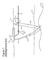
- a vessel 100 tows an array of seismic detectors 112 provided along cables 114.
- the detectors and cables form streamers 116.
- Streamers 116 may be disposed horizontally, i.e., lie at a constant depth z1 relative to the surface 118 of the ocean, or they may be tilted in relation to this surface.
- Vessel 100 also tows a sound source 120 configured to generate an acoustic wave 122a.
- Acoustic wave 122a propagates downward, toward seafloor 124, and penetrates it until eventually a reflecting structure 126 (reflector) reflects the acoustic wave.
- the reflected acoustic wave 122b propagates upward until it is detected by detector 112.
- the recorded data is then processed to produce an accurate image of the subsurface.
- Processing includes various phases, e.g., velocity model determination, pre-stack, migration, post-stack, etc., which are known in the art, so their description is omitted herein.
- Progress in pre-stack depth imaging has been considerable in the past. Theoretical progress has provided better methods for extrapolating wavefields measured at the earth's surface into the subsurface, and practical progress has linked the migrations more closely with velocity model-building and interpretation.
- Migration is the process of propagating, for example, a wavefield measured at a receiver location to a reflector located in the subsurface. Migration may also be applied to wavefields generated by a source.
- LSM least-squares migration
- RTM and RTDM take advantage of a complete set of acoustic waves (reflections, transmissions, diffractions, prismatic waves, etc.), correctly handle complex velocities, and propagate waves without angle limitations. For these reasons, RTM and RTDM are desirable as the imaging and modeling operators in least-squares RTM (LSRTM). The modeling uses velocity and density as the input models.
- the method includes receiving measured seismic data d of the subsurface; selecting an objective function E that is function of a reflectivity r of the subsurface, wherein the objective function E includes a term that cross-correlates the measured seismic data d and simulated data d at zero lag; calculating the reflectivity r based on the measured seismic data d, objective function E, and simulated data d; and generating the final image based on reflectivity r.
- a method for generating a final image of a subsurface of the earth includes receiving measured seismic data d of the subsurface; selecting an objective function E that is function of a reflectivity r of the subsurface, wherein the objective function E includes a term that cross-correlates the measured seismic data d and simulated data d at zero lag; and calculating, in a processor, the reflectivity r based on the measured seismic data d, objective function E, simulated data d, a modeling operator M from a reverse time demigration (RTDM) process and an imaging operator M T from a reverse time migration (RTM) process.
- RTDM reverse time demigration
- RTM reverse time migration
- a new general framework of LSRTM is introduced and is based on maximizing a cross-correlation of simulated and observed seismic data at zero lag.
- the new method relaxes the amplitude constraints and, thus, it can be applied to actual data and shows improved stability performance compared to LSRTM.
- the new method is called correlative least-squares RTM (CLSRTM).
- CLSRTM correlative least-squares RTM
- a Newton's method may be applied to solve it.
- other mathematical algorithms may be applied. Both synthetic and real numerical results (presented later) show that CLSRTM leads to improved image quality, revealing more structural detail in areas of poor illumination and imaging.
- f(t) is the source signature
- ⁇ ( x ) is the velocity of the medium
- ⁇ ( x ) is the medium's density
- ⁇ ⁇ ⁇ x ⁇
- the aim is to reconstruct the wavefield recorded at the receivers based on a given stacked image I ( x ), migration velocity ⁇ ( x ) and source location x s .
- I ( x ) migration velocity
- ⁇ ( x ) migration velocity
- source location x s source location
- objective function E is an integral of the cross-correlation between the modeled seismic data Mr and the reflectivity model r over the source and sensors' positions. Note that objective function E is a function of reflectivity model r.
- the CLSRTM method finds an optimal image r which maximizes the cross-correlation between seismic data d and simulated data Mr at zero lag, or equivalently, minimizes objective function E. If the two datasets d and Mr are identical or different by a constant scaling, the objective function reaches its minimum at -1.
- a numerical solution can be found, for example, using Newton's method, which uses the gradient and Hessian of the objective function.
- dE d M ⁇ ⁇ r 1 ⁇ d ⁇ ⁇ Mr ⁇ ⁇ f ⁇ Mr ⁇ d ⁇ dt ⁇ Mr ⁇ 2 ⁇ Mr - d
- step 200 of Figure 2 recorded data d is received. This data may be recorded using a marine or land seismic acquisition system.
- objective function E and a stopping criterion are checked, for example, against a predetermined value.
- the predetermined value may be -0.9 and the stopping criterion is whether E is smaller than -0.9.
- Other values for the predetermined value may be selected, based, for example, on the nature, conditions, and goals of the survey.
- step 216 For example, if a salt or chalk region is expected to cover the surveyed subsurface, this value may be changed. If the stopping criterion is met, then the process returns to step 206 and repeats steps 206-214 discussed above. Otherwise, the process generates optimal image r in step 216.
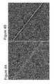
- Figure 4A illustrates the inverted image obtained using a conventional RTM method that includes migration artifacts and crosstalk noise 400
- Migration artifacts and crosstalk noise 400 associated with multiple sources are suppressed in Figure 4B , and wavelet 402 at the dipping reflector is better focused and appears much sharper compared with the initial RTM image ( Figure 4A ) using the same recorded data.
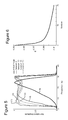
- FIG. 5 shows the frequency spectrum of the inverted amplitudes on the dipping reflector for every 5 th iteration (I0 is the initial image, 15 corresponds to the 5 th iteration, 110 corresponds to the 10 th iteration, 115 corresponds to the 15 th iteration and 120 corresponds to the 20 th iteration), and Figure 6 shows the numerical value of objective function E for every iteration during the 20 iterations.
- This example includes the 2D synthetic data set Sigsbee2A disclosed in Paffenholz et al., 2002, "Subsalt multiple attenuation and imaging: Observations from the Sigsbee2B synthetic dataset," 72nd Annual International Meeting, SEG, Expanded Abstracts, 2122-2125 , the entire content of which is included herein by reference.
- the seismic data is generated using a (fine) stratigraphic velocity model, with 50 m shot spacing, 25 m receiver spacing and 8,500 m maximum offset. Both source and receiver ghosts are recorded at 8.5 m depth.
- the seismic data is first migrated using the (smoothed) migration velocity. As illustrated in Figure 7A , the initial simulated data does not match well the actual seismic data illustrated in Figure 7C , due to acquisition limitations and the imperfection of the imaging operator. However, over a number of iterations of the CLSRTM method, the simulated data illustrated in Figure 7B gradually approaches the actual seismic data of Figure 7C .
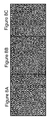
- Figures 8A-C illustrate the initial RTM image ( Figure 8A ), the inverted image after 10 iterations of the CLSRTM method using migration velocity ( Figure 8B ), and using stratigraphic velocity ( Figure 8C ).
- the sedimentary structure on the left of the image is much sharper because of the deghosting effect intrinsically built into the CLSRTM method, while the subsalt structures are enhanced to give a better overall amplitude balance.
- the equally-spaced diffractors artificially put into the velocity model also provide references that the focusing in the inverted image is improved.
- FIGS 9A-B A third and final example is illustrated in Figures 9A-B .
- Real seismic data from the central North Sea is illustrated in these examples.
- the seismic data has been bandpass filtered from 5Hz to 45Hz, and regularized to a 50 m by 50 m receiver grid.
- the migration model is TTI (Tilted Transverse Isotropy).
- CLSRTM Standard Transverse Isotropy
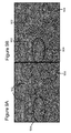
- a salt dome 900 is presented in the center, but its steeply dipping flanks 902 are weakly imaged.
- the CLSRTM method provides stable solutions even when the source signature is unknown. Because RTDM can simulate data with free surface boundary conditions for any acquisition, the CLSRTM method is capable of handling some of the difficult imaging issues caused by acquisition, such as free surface ghosts for towed streamers and crosstalk caused by simultaneous shooting.
- step 1000 measured seismic data d is received at a computing device for processing.
- An objective function E for example, the one defined in equation (6), is selected in step 1002.
- another objective function E may be selected that describes a cross-correlation between the measured seismic data d and simulated data.
- objective function E is a function of image r, which is mathematically expressed as E(r).
- a gradient and hessian of the objective function may be calculated if a Newton method is applied for calculating optimal image r.
- Other mathematical methods may be selected to calculate optimal image r as will be appreciated by those skilled in the art.
- initial reflectivity image r 0 and initial simulated data do may be calculated using the RTM algorithm. Other algorithms may be used to calculate these initial quantities.
- step 1006 an iteration index is updated for each iteration.
- step 1008 for calculating a gradient direction in the image domain ⁇ r i , where ⁇ r i is given by equation (10).
- step 1010 the modeling operator M of the RTDM process is applied to gradient direction ⁇ r i to obtain equation (11).
- a Newton update is performed on the simulated seismic data using equation (12) and inverted image using equation (13).
- scalar ⁇ is found by maximizing objective function E selected in step 1002, for example, using a linear searching method.
- objective function E is checked and a stopping criterion (e.g., E ⁇ -0.9) is verified. Note that other stopping criterion may be used, depending on the survey, its goals, the structure of the subsurface, etc. If the stopping criterion is not satisfied, the process returns to step 1006 to perform another iteration. However, if the condition is satisfied, the process generates the optimal image r in step 1016. Based on this, a final image of the surveyed subsurface may be displayed in step 1018.
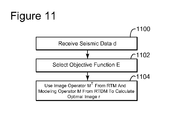
- step 1100 measured seismic data d is received.
- the measured seismic data may be supplemented with observed seismic data d, initial reflectivity image r 0 and initial simulated data do.
- an objective function E is selected that reflects a cross-correlation between the measured seismic data d and the simulated data.
- step 1104 an optimal image r is calculated by using the image operator from RTM and the modeling operator from RTDM to maximize/minimize objective function E.
- the curved streamer 1200 of Figure 12 includes a body 1202 having a predetermined length, plural detectors 1204 provided along the body, and plural birds 1206 provided along the body to maintain the selected curved profile.
- the streamer is configured to flow underwater when towed such that the plural detectors are distributed along the curved profile.
- the curved profile may be described as a parameterized curve, e.g., a curve described by (i) a depth z0 of a first detector (measured from the water surface 1212), (ii) a slope s0 of a first portion T of the body with an axis 1214 parallel with the water surface 1212, and (iii) a predetermined horizontal distance hc between the first detector and an end of the curved profile.
- the curved profile should not be construed to always apply to the entire length of the streamer. While this situation is possible, the curved profile may be applied only to a portion 1208 of the streamer. In other words, the streamer may have (i) only a portion 1208 having the curved profile or (ii) a portion 1208 having the curved profile and a portion 1210 having a flat profile, with the two portions attached to each other.
- a multi-level source 1300 has one or more sub-arrays.
- the first sub-array 1302 has a float 1306 configured to float at the water surface 1308 or underwater at a predetermined depth.
- Plural source points 1310a-d are suspended from the float 1306 in a known manner.
- a first source point 1310a may be suspended closest to the head 1306a of float 1306, at a first depth z1.
- a second source point 1310b may be suspended next, at a second depth z2, different from z1.
- a third source point 1310c may be suspended next, at a third depth z3, different from z1 and z2, and so on.
- Figure 13 shows, for simplicity, only four source points 1310a-d, but an actual implementation may have any desired number of source points.
- the source points are distributed at different depths, these source points are not simultaneously activated.
- the source array is synchronized, i.e., a deeper source point is activated later in time (e.g., 2 ms for 3 m depth difference when the speed of sound in water is 1,500 m/s) such that corresponding sound signals produced by the plural source points coalesce and, thus, the overall sound signal produced by the source array appears to be a single sound signal.
- Depths z1 to z4 of the source points of the first sub-array 1302 may obey various relationships.
- the source points' depths increase from the head toward the tail of the float, i.e., z1 ⁇ z2 ⁇ z3 ⁇ z4.
- the source points' depths decrease from the head to the tail of the float.
- the source points are slanted, i.e., provided on an imaginary line 1314.
- line 1314 is straight.
- line 1314 is curved, e.g., part of a parabola, circle, hyperbola, etc.
- the depth of the first source point for sub-array 1302 is about 5 m and the greatest depth of the last source point is about 8 m.
- the depth range is between 8.5 and 10.5 m or between 11 and 14 m.
- the source points's depths increase by 0.5 m from one source point to an adjacent source point.
- Processing device 1400 may be specifically configured to calculate an optimal image r for use in generating a final image of a subsurface of the earth.
- Processing device 1400 may be, for example, a computer, a processor, a server, or a network of computers, processors or servers.
- Processing device 1400 may include an interface 1402 configured to receive data from outside, e.g., seismic data. Interface 1402 may accommodate an Internet connection, satellite connection, keyboards, etc.
- Processing device 1400 also includes a processor 1404 connected to interface 1402 through a bus 1406 and configured to execute one or more or all of the steps discussed with regard to Figures 2 , 10 and 11 .
- Processing device 1400 may have dedicated circuitry for each step of Figures 2 , 10 and 11 or processor 1404 may be configured with software to execute all the steps shown in these figures. Processing device 1400 may also include a display 1408 for displaying a final image calculated by processor 1404. Various data used for calculating the final image may be stored in a storage device 1410 connected to processor 1404. Other known components of a computer, server or processor may also be present.
- the disclosed exemplary embodiments provide a system and a method for processing, with fast convergence, data related to a subsurface. It should be understood that this description is not intended to limit the invention. On the contrary, the exemplary embodiments are intended to cover alternatives, modifications and equivalents, which are included in the spirit and scope of the invention as defined by the appended claims. Further, in the detailed description of the exemplary embodiments, numerous specific details are set forth in order to provide a comprehensive understanding of the claimed invention. However, one skilled in the art would understand that various embodiments may be practiced without such specific details.
Landscapes
- Engineering & Computer Science (AREA)
- Remote Sensing (AREA)
- Physics & Mathematics (AREA)
- Life Sciences & Earth Sciences (AREA)
- Acoustics & Sound (AREA)
- Environmental & Geological Engineering (AREA)
- Geology (AREA)
- General Life Sciences & Earth Sciences (AREA)
- General Physics & Mathematics (AREA)
- Geophysics (AREA)
- Geophysics And Detection Of Objects (AREA)
Abstract
Description
- This application claims priority and benefit from United States Provisional Patent Application No.
61/807,950, filed April 3, 2013 - Embodiments of the subject matter disclosed herein generally relate to methods and systems and, more particularly, to mechanisms and techniques for providing high-quality images of a surveyed subsurface, with balanced amplitudes, improved focusing and enhanced resolution.
- Marine seismic data acquisition and processing generate a profile (image) of the geophysical structure under the seafloor. While this profile does not provide an accurate location for oil and gas reservoirs, it suggests, to those trained in the field, the presence or absence of them. Thus, providing a high-resolution image of the structures under the seafloor is an ongoing process.
- During a seismic gathering process, as shown in
Figure 1 , avessel 100 tows an array ofseismic detectors 112 provided along cables 114. The detectors and cables formstreamers 116.Streamers 116 may be disposed horizontally, i.e., lie at a constant depth z1 relative to thesurface 118 of the ocean, or they may be tilted in relation to this surface. Vessel 100 also tows asound source 120 configured to generate anacoustic wave 122a.Acoustic wave 122a propagates downward, towardseafloor 124, and penetrates it until eventually a reflecting structure 126 (reflector) reflects the acoustic wave. The reflectedacoustic wave 122b propagates upward until it is detected bydetector 112. The recorded data is then processed to produce an accurate image of the subsurface. - Processing includes various phases, e.g., velocity model determination, pre-stack, migration, post-stack, etc., which are known in the art, so their description is omitted herein. Progress in pre-stack depth imaging has been considerable in the past. Theoretical progress has provided better methods for extrapolating wavefields measured at the earth's surface into the subsurface, and practical progress has linked the migrations more closely with velocity model-building and interpretation. Migration is the process of propagating, for example, a wavefield measured at a receiver location to a reflector located in the subsurface. Migration may also be applied to wavefields generated by a source.
- Initial migration methods (Kirchhoff and beam) relied on rays to approximate the Green's functions for wave propagation. More accurate methods rely on the so-called wave-equation migration algorithms that use full waveform Green's functions. The most computationally efficient algorithms for doing this are collectively called one-way wave equation migration (OWEM). These algorithms decompose seismic wavefields inside the earth into up-going waves and down-going waves under the assumption of no interaction between these two wavefields; that is, no turning wave and vertical reflection generation during the synthesis of wave propagation.
- Use of the two-way wave equation in depth migration began some time ago in an algorithm called reverse-time migration (RTM), see, for example, Zhang and Sun, 2009, "Practical issues of reverse time migration: true-amplitude gathers, noise removal and harmonic-source encoding," First Break, Vol. 26, 19-25, and Xu et al., 2011, "3D angle gathers from reverse time migration," Geophysics, Vol. 76, No. 2, S77-S92, the entire contents of which are incorporated herein by reference.
- However, this approach was limited due to its need for computer power. With increases in computer power, RTM has developed rapidly over the last few years, and theoretical advantages such as dip-unlimited accurate wave propagation and improved amplitudes have provided imaging benefits in practice. For example, in complex subsalt and salt flank areas, the numerical Green's functions from finite difference to the two-way wave equation have better amplitude behavior, so it is easier to incorporate amplitude corrections into RTM than into OWEM. In addition to its ability to handle complex velocities distributions, many current RTM algorithms can handle anisotropic media such as vertical transverse isotropy (VTI) and tilted transverse isotropy (TTI).
- One of the most common RTM imaging conditions is cross-correlation of the forward propagated source wavefield with the backward propagated receiver wavefield. However, the image contains amplitude distortions caused by RTM crosstalk artifacts. An inversion-based least-squares migration (LSM) scheme has been shown to noticeably reduce migration artifacts and improve lateral spatial resolution. LSM iteratively seeks a final image which best matches the amplitude of simulated and recorded seismic data. This final image is thus called the inverted image. However, the forward modeling and migration engine for the LSM scheme were in the past the Kirchhoff migration, which suffers from the limitations noted above. Recently, one-wave wave equation and two-way RTM were used as the modeling and migration engine.
- More recently, true-amplitude RTM became the state-of-the-art technology for imaging and interpreting subtle and complex geologic features, while its conjugate process, reverse-time demigration (RTDM) (see, for example, Zhang and Duan, 2012, "Predicting multiples using a reverse time demigration," 83rd Annual International Meeting, SEG, Expanded Abstracts, 520-524, the entire content of which is incorporated herein by reference), has become a novel technique to predict primary, interbed and surface-related multiples and free surface ghosts for a variety of acquisition geometries. Demigration is considered the inverse of the adjoint process of migration. Demigration uses reflectivity to predict seismic data. Both techniques, RTM and RTDM, take advantage of a complete set of acoustic waves (reflections, transmissions, diffractions, prismatic waves, etc.), correctly handle complex velocities, and propagate waves without angle limitations. For these reasons, RTM and RTDM are desirable as the imaging and modeling operators in least-squares RTM (LSRTM). The modeling uses velocity and density as the input models.
- However, it is not an easy task to directly apply conventional amplitude-matching-based LSRTM to real datasets because the earth is a viscoelastic medium with density variations, much more complicated than the models used to propagate acoustic wavefields in seismic imaging. As a result, amplitude matching is never perfect. Also, it is difficult to define a good source signature in the modeling. The challenge of determining source strength, which can vary from source to source, is even greater. All these practical issues require considerable effort in preprocessing both the observed and simulated data to correctly use the conventional LSRTM formulation.
- Thus, it is desirable to introduce a new general framework of LSRTM that avoids the above-noted problems and relaxes the amplitude constraints of existing LSRTM.
- According to one exemplary embodiment, there is a method for generating a final image of a subsurface of the earth. The method includes receiving measured seismic data d of the subsurface; selecting an objective function E that is function of a reflectivity r of the subsurface, wherein the objective function E includes a term that cross-correlates the measured seismic data d and simulated data d at zero lag; calculating the reflectivity r based on the measured seismic data d, objective function E, and simulated data d; and generating the final image based on reflectivity r.
- According to another embodiment, there is a method for generating a final image of a subsurface of the earth. The method includes receiving measured seismic data d of the subsurface; selecting an objective function E that is function of a reflectivity r of the subsurface, wherein the objective function E includes a term that cross-correlates the measured seismic data d and simulated data d at zero lag; and calculating, in a processor, the reflectivity r based on the measured seismic data d, objective function E, simulated data d, a modeling operator M from a reverse time demigration (RTDM) process and an imaging operator MT from a reverse time migration (RTM) process.
- According to still another exemplary embodiment, there is a method for generating a final image of a subsurface of the earth. The method includes receiving measured seismic data d of the subsurface; selecting an objective function E that is function of a reflectivity r of the subsurface; and calculating, in a processor, the reflectivity r based on the measured seismic data d, the objective function E, simulated data d, a modeling operator M from a reverse time demigration (RTDM) process and an imaging operator MT from a reverse time migration (RTM) process.
- The accompanying drawings, which are incorporated in and constitute a part of the specification, illustrate one or more embodiments and, together with the description, explain these embodiments. In the drawings:
-
Figure 1 is a schematic diagram of a conventional data acquisition setup; -
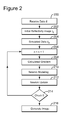
Figure 2 is a flowchart of a correlative least-squares RTM method; -
Figure 3A is a graph illustrating an exact density model; -
Figure 3B is a shot record of simultaneous shooting; -
Figure 4A is an image of a surveyed subsurface obtained by applying an RTM algorithm; -
Figure 4B is an image of the surveyed subsurface obtained by applying the correlative least-squares RTM algorithm; -
Figure 5 illustrates frequency spectrum variations of a dipping reflector; -
Figure 6 illustrates the value of an objective function as a function of a number of iterations; -
Figure 7A illustrates an initial simulated shot record,Figure 7B illustrates the same shot location calculated with the correlative least-squares RTM, andFigure 7C illustrates the same shot location based on the recorded seismic data; -
Figure 8A illustrates an image of a simulated subsurface using the RTM method,Figure 8B illustrates the same subsurface using the correlative least-squares RTM, andFigure 8C illustrates the same subsurface using a stratigraphic velocity; -
Figure 9A illustrates an image of a surveyed subsurface using the RTM algorithm, andFigure 9B illustrates the same subsurface using the correlative least-squares RTM; -
Figure 10 is a flowchart illustrating the correlative least-squares RTM; -
Figure 11 is another flowchart illustrating the correlative least-squares RTM; -
Figure 12 is a schematic diagram of a curved streamer; -
Figure 13 is a schematic diagram of a multi-component source; and -
Figure 14 is a schematic diagram of a computing device. - The following description of the exemplary embodiments refers to the accompanying drawings. The same reference numbers in different drawings identify the same or similar elements. The following detailed description does not limit the invention. Instead, the scope of the invention is defined by the appended claims. The following embodiments are discussed, for simplicity, with regard to the terminology of source wavefields, receiver wavefields, RTM, RTDM and LSM methods in the context of marine seismic data processing. However, the embodiments to be discussed next are not limited to marine seismic data or RTM and RTDM methods, but may be applied to other type of data, e.g., seismic land data and/or other methods and operators, e.g., Kirchhoff.
- Reference throughout the specification to "one embodiment" or "an embodiment" means that a particular feature, structure or characteristic described in connection with an embodiment is included in at least one embodiment of the subject matter disclosed. Thus, the appearance of the phrases "in one embodiment" or "in an embodiment" in various places throughout the specification is not necessarily referring to the same embodiment. Further, the particular features, structures or characteristics may be combined in any suitable manner in one or more embodiments.
- According to an embodiment, a new general framework of LSRTM is introduced and is based on maximizing a cross-correlation of simulated and observed seismic data at zero lag. The new method relaxes the amplitude constraints and, thus, it can be applied to actual data and shows improved stability performance compared to LSRTM. The new method is called correlative least-squares RTM (CLSRTM). To improve numerical convergence, a Newton's method may be applied to solve it. However, other mathematical algorithms may be applied. Both synthetic and real numerical results (presented later) show that CLSRTM leads to improved image quality, revealing more structural detail in areas of poor illumination and imaging.
- Before discussing the details of the CLSRTM method, a few general seismic concepts are introduced to facilitate understanding of the new method. If the simulated seismic data is d and the reflectivity model is m, a forward modeling operator L connects the seismic data to the reflectivity model as described by equation (1):

- The migration operator is the adjoint of the forward modeling operator L and can be represented by:

where mmig is the migration image. To obtain a better reflectivity image, a least-squares inversion problem may be used, i.e., an objective function O(m) may be defined as the least-squares difference between the forward modeled data Lm and the recorded data d:
- Note that after calculating a source wavefield PS (originating at the source location) and a receiver wavefield PR (recorded at the receivers) with the RTM method, the angle-dependent reflectivity r, at a subsurface reflection point
x , is given by r(x ; θ) = ∫PR(x , t)/PS(x , t) dt, and the stacked image I can be expressed as I(x ) =∬PR(x ,t)/PS(x ,t)dtdθ. - With this general background in mind, the novel method is now discussed. To simplify presentation of the CLSRTM method, it is assumed that the earth is an isotropic medium. However, note that the novel method is also applicable to a non-isotropic earth. With this assumption, a wavefield P(
x ; t) can be modeled by the acoustic wave equation as follows:
where f(t) is the source signature, ν(x ) is the velocity of the medium, ρ(x ) is the medium's density,
x r due to specified source locationx s. - In RTDM, which is described below by equations (5a-c), the aim is to reconstruct the wavefield recorded at the receivers based on a given stacked image I(
x ), migration velocity ν(x ) and source locationx s. For example, it is possible to predict the recorded seismic data from the stacked image, or reflectivity model r(x ), using the following partial differential equations:
with PR being the receiver wavefield, PS being the source wavefield and d being the estimated seismic data. - Note that receiver wavefield PR(
x ; t) propagates only waves generated by fictitious sources that result from the multiplication of source wavefield PS(x ; t) and reflectivity r(x ) in equation (5b). - The LSRTM method tries to match simulated data d (obtained in equation 5c) with observed (measured) data d. Even in the ideal situation where the exact velocity and source information are known, e.g., ν̃=ν and f = f, the RTDM (described by equations (5a-c) above) and the RTM (described by equations (4a-b) above) produce different propagation amplitudes. When the source information is absent or the demigration velocity is inexact, the data matching step using only the amplitude information becomes even more challenging.
- Thus, LSRTM suffers because of the rigid amplitude matching condition. An alternative approach to LSRTM is to relax the amplitude matching condition and to measure the closeness between the simulated data and the seismic data. To evaluate the above-noted closeness, a cross-correlation-based objective function E may be introduced. This novel objective function alleviates the rigid amplitude matching step in LSRTM. For example, in one embodiment, in the time domain, cross-correlation-based objective function E may take the form:

where M is the modeling operator from RTDM, Mr (or d) is the modeled seismic data, and the negative sign on the right-hand side of the equal sign is introduced so the optimal solution is achieved when objective function E(r) reaches its minimum (or maximum). In one application, objective function E is an integral of the cross-correlation between the modeled seismic data Mr and the reflectivity model r over the source and sensors' positions. Note that objective function E is a function of reflectivity model r. - In CLSRTM, the velocity model, which is embedded in modeling operator M, is assumed to be corrected or already optimized. Note that the value of E(r) is unchanged by rescaling modeled seismic data Mr. Therefore, the exact overall scaling of the source strength can be ignored in CLSRTM, which is an advantage over existing algorithms.
- The CLSRTM method finds an optimal image r which maximizes the cross-correlation between seismic data d and simulated data Mr at zero lag, or equivalently, minimizes objective function E. If the two datasets d and Mr are identical or different by a constant scaling, the objective function reaches its minimum at -1. A numerical solution can be found, for example, using Newton's method, which uses the gradient and Hessian of the objective function. A small perturbation of the reflectivity image δr may be applied to objective function E, as follows:

where ||·|| is the L2 norm. Applying a Taylor expansion, the gradient is found to be given by:
and the Hessian is given by:
- Simulated data d and actual data d are then matched using the gradient calculated in equation (8) and the Hessian calculated in equation (9). A flowchart of the CLSRTM method is now discussed with respect to
Figure 2 . - In
step 200 ofFigure 2 , recorded data d is received. This data may be recorded using a marine or land seismic acquisition system. Instep 202, an initial reflectivity image r0 is assumed to be known. Simulated initial data do = Mr0 is calculated instep 204, for example, using the RTM algorithm. Then, an iteration index "n" is initiated and an iterative process is started instep 206, followed by the calculation instep 208 of the gradient direction δri in the image domain based on equation:
where "T" stands for the transpose operation and MT is the RTM imaging operator. - Next, the process advances to step 210, in which is performed seismic modeling M of the gradient direction δri:

- A Newton algorithm is applied in
step 212 on simulated seismic data using equation:
and on the inverted image using equation:
where scalar α is found by minimizing objective function E using a linear searching method. Instep 214, objective function E and a stopping criterion are checked, for example, against a predetermined value. For example, the predetermined value may be -0.9 and the stopping criterion is whether E is smaller than -0.9. Other values for the predetermined value may be selected, based, for example, on the nature, conditions, and goals of the survey. For example, if a salt or chalk region is expected to cover the surveyed subsurface, this value may be changed. If the stopping criterion is met, then the process returns to step 206 and repeats steps 206-214 discussed above. Otherwise, the process generates optimal image r instep 216. - The above-discussed method is now applied to a set of synthetic data and then to a set of real data for illustrating its power. For the synthetic data, consider the situation in which three identical sources are shooting simultaneously, i.e., they are firing at the same time with source depth of 12.5 m and source separations of 1 km. Streamer cables are towed in between these three sources at the same depth, and both shot and receiver ghosts are recorded. Setting the background velocity to 2 km/s and the density model to contain a dipping reflector as illustrated in
Figure 3A , an acoustic modeling code is used to generate the seismic data. In CLSRTM, knowledge is assumed of the source wavelet and the use of RTDM to simulate seismic data with ghosts as illustrated inFigure 3B .Figure 4A illustrates the inverted image obtained using a conventional RTM method that includes migration artifacts andcrosstalk noise 400, whileFigure 4B illustrates the inverted image at the end of iteration n=20 (seeFigure 2 , step 206) of the CLSRTM method. Migration artifacts andcrosstalk noise 400 associated with multiple sources are suppressed inFigure 4B , andwavelet 402 at the dipping reflector is better focused and appears much sharper compared with the initial RTM image (Figure 4A ) using the same recorded data. - This side-by-side comparison of the inverted image obtained with the traditional RTM method and the new CLSRTM method shows that CLSRTM gradually removes ghost effects over the iterations and gives wider and more balanced frequency bandwidth.
Figure 5 shows the frequency spectrum of the inverted amplitudes on the dipping reflector for every 5th iteration (I0 is the initial image, 15 corresponds to the 5th iteration, 110 corresponds to the 10th iteration, 115 corresponds to the 15th iteration and 120 corresponds to the 20th iteration), andFigure 6 shows the numerical value of objective function E for every iteration during the 20 iterations. While the amplitude spectra indicate a gradual deghosting process over the iterations, converging to the correct solution with flat spectrum from 0 to 32 Hz, the value of the objective function decreases rapidly for the first several iterations, and then steadily improves for the later iterations. - Next, another synthetic example is processed with the CLSRTM method. This example includes the 2D synthetic data set Sigsbee2A disclosed in Paffenholz et al., 2002, "Subsalt multiple attenuation and imaging: Observations from the Sigsbee2B synthetic dataset," 72nd Annual International Meeting, SEG, Expanded Abstracts, 2122-2125, the entire content of which is included herein by reference.
- The seismic data is generated using a (fine) stratigraphic velocity model, with 50 m shot spacing, 25 m receiver spacing and 8,500 m maximum offset. Both source and receiver ghosts are recorded at 8.5 m depth. The seismic data is first migrated using the (smoothed) migration velocity. As illustrated in
Figure 7A , the initial simulated data does not match well the actual seismic data illustrated inFigure 7C , due to acquisition limitations and the imperfection of the imaging operator. However, over a number of iterations of the CLSRTM method, the simulated data illustrated inFigure 7B gradually approaches the actual seismic data ofFigure 7C . For example, inFigures 7A-C , some reflections (marked with arrow 700) which are weak on the initial simulated data (Figure 7A ) but strong on the actual seismic data (Figure 7C ), are enhanced after 10 iterations of the CLSRTM method (Figure 7B ). This demonstrates that the novel CLSRTM method, based on the cross-correlation objective function, works better than existing methods to match the seismic data by updating the reflectivity model. - For the same synthetic example,
Figures 8A-C illustrate the initial RTM image (Figure 8A ), the inverted image after 10 iterations of the CLSRTM method using migration velocity (Figure 8B ), and using stratigraphic velocity (Figure 8C ). The sedimentary structure on the left of the image is much sharper because of the deghosting effect intrinsically built into the CLSRTM method, while the subsalt structures are enhanced to give a better overall amplitude balance. The equally-spaced diffractors artificially put into the velocity model also provide references that the focusing in the inverted image is improved. - Some artifacts are observed in the sediments above the salt after applying the CLSRTM method. Using the (exact) stratigraphic velocity in the imaging operator of the CLSRTM method results in improved image quality in
Figure 8C for the 10th iteration, and the migration artifacts above the salt are reduced. A close comparison shows the structures and diffractors in the subsalt area are also better focused using the correct velocity. These figures suggest that, although CLSRTM can tolerate a certain amount of velocity inaccuracy, a good velocity model is still desirable to unlock the structures, especially when geology is complicated. - A third and final example is illustrated in
Figures 9A-B . Real seismic data from the central North Sea is illustrated in these examples. The seismic data has been bandpass filtered from 5Hz to 45Hz, and regularized to a 50 m by 50 m receiver grid. The migration model is TTI (Tilted Transverse Isotropy). Using the CLSRTM method, it is assumed that the source signature is unknown for both imaging and modeling and, by default, a source as a bandlimited flat spectrum wavelet is introduced. In the initial RTM image illustrated inFigure 9A , asalt dome 900 is presented in the center, but its steeply dippingflanks 902 are weakly imaged. After 9 iterations of the CLSRTM method, illumination of the image near the salt dome boundary is enhanced as illustrated inFigure 9B , showing strong energy on the nearly-vertical salt flanks and the termination structures, compared with the initial image. In addition, illumination of thechalk section 904 on either side of the salt in the inverted image is improved. In many places, the structures become more continuous. Overall, the inverted image using the CLSRTM method is amplitude-balanced with improved continuity and reveals more detailed structures. - Based on the above-discussed examples, least-squares migration is an attractive technique for improving image resolution and illumination, and suppressing migration artifacts. By using a cross-correlation objective function, the CLSRTM method provides stable solutions even when the source signature is unknown. Because RTDM can simulate data with free surface boundary conditions for any acquisition, the CLSRTM method is capable of handling some of the difficult imaging issues caused by acquisition, such as free surface ghosts for towed streamers and crosstalk caused by simultaneous shooting.
- The novel methods discussed above may be implemented, in one embodiment, as now illustrated in
Figure 10 . An objective of the process now described is to find the optimal image r that maximizes the cross-correlation between measured seismic data d and simulated data Mr at zero lag. Thus, instep 1000, measured seismic data d is received at a computing device for processing. An objective function E, for example, the one defined in equation (6), is selected instep 1002. Note that another objective function E may be selected that describes a cross-correlation between the measured seismic data d and simulated data. In other words, objective function E is a function of image r, which is mathematically expressed as E(r). In the same step, a gradient and hessian of the objective function may be calculated if a Newton method is applied for calculating optimal image r. Other mathematical methods may be selected to calculate optimal image r as will be appreciated by those skilled in the art. - In
step 1004, an initial reflectivity image r0 and initial simulated data do = Mr0 are assumed to be known, where M is the modeling operator from the RTDM. In one application, initial reflectivity image r0 and initial simulated data do may be calculated using the RTM algorithm. Other algorithms may be used to calculate these initial quantities. Having these initial quantities, the process advances to step 1006, where an iteration index is updated for each iteration. For each iteration, the process advances to step 1008 for calculating a gradient direction in the image domain δri, where δri is given by equation (10). - In
step 1010, the modeling operator M of the RTDM process is applied to gradient direction δri to obtain equation (11). Instep 1012, a Newton update is performed on the simulated seismic data using equation (12) and inverted image using equation (13). - For updating the simulated seismic data d and inverted image r, scalar α is found by maximizing objective function E selected in
step 1002, for example, using a linear searching method. Instep 1014 objective function E is checked and a stopping criterion (e.g., E < -0.9) is verified. Note that other stopping criterion may be used, depending on the survey, its goals, the structure of the subsurface, etc. If the stopping criterion is not satisfied, the process returns to step 1006 to perform another iteration. However, if the condition is satisfied, the process generates the optimal image r instep 1016. Based on this, a final image of the surveyed subsurface may be displayed instep 1018. - The process discussed above with regard to
Figure 10 provides many details for implementing the novel methods in a given computing device. The same process may also be expressed, as now discussed with regard toFigure 11 , with less detail so as not to obscure some of the novel features. Instep 1100, measured seismic data d is received. The measured seismic data may be supplemented with observed seismic data d, initial reflectivity image r0 and initial simulated data do. Instep 1102, an objective function E is selected that reflects a cross-correlation between the measured seismic data d and the simulated data. Instep 1104, an optimal image r is calculated by using the image operator from RTM and the modeling operator from RTDM to maximize/minimize objective function E. - The above embodiments were discussed without specifying what type of seismic receivers is used to record the seismic data. In this sense, it is known in the art to use, for a marine seismic survey, streamers that include seismic receivers, which are towed by one or more vessels. The streamers may be horizontal, slanted or have a curved profile as illustrated in
Figure 12 . - The
curved streamer 1200 ofFigure 12 includes abody 1202 having a predetermined length,plural detectors 1204 provided along the body, andplural birds 1206 provided along the body to maintain the selected curved profile. The streamer is configured to flow underwater when towed such that the plural detectors are distributed along the curved profile. The curved profile may be described as a parameterized curve, e.g., a curve described by (i) a depth z0 of a first detector (measured from the water surface 1212), (ii) a slope s0 of a first portion T of the body with anaxis 1214 parallel with thewater surface 1212, and (iii) a predetermined horizontal distance hc between the first detector and an end of the curved profile. Note that not the entire streamer has to have the curved profile. In other words, the curved profile should not be construed to always apply to the entire length of the streamer. While this situation is possible, the curved profile may be applied only to aportion 1208 of the streamer. In other words, the streamer may have (i) only aportion 1208 having the curved profile or (ii) aportion 1208 having the curved profile and aportion 1210 having a flat profile, with the two portions attached to each other. - Further, the above embodiments may be used with a multi-level source. A
multi-level source 1300 has one or more sub-arrays. The first sub-array 1302 has afloat 1306 configured to float at thewater surface 1308 or underwater at a predetermined depth. Plural source points 1310a-d are suspended from thefloat 1306 in a known manner. Afirst source point 1310a may be suspended closest to thehead 1306a offloat 1306, at a first depth z1. Asecond source point 1310b may be suspended next, at a second depth z2, different from z1. Athird source point 1310c may be suspended next, at a third depth z3, different from z1 and z2, and so on.Figure 13 shows, for simplicity, only foursource points 1310a-d, but an actual implementation may have any desired number of source points. In one application, because the source points are distributed at different depths, these source points are not simultaneously activated. In other words, the source array is synchronized, i.e., a deeper source point is activated later in time (e.g., 2 ms for 3 m depth difference when the speed of sound in water is 1,500 m/s) such that corresponding sound signals produced by the plural source points coalesce and, thus, the overall sound signal produced by the source array appears to be a single sound signal. - Depths z1 to z4 of the source points of the first sub-array 1302 may obey various relationships. In one application, the source points' depths increase from the head toward the tail of the float, i.e., z1 <z2<z3<z4. In another application, the source points' depths decrease from the head to the tail of the float. In another application, the source points are slanted, i.e., provided on an
imaginary line 1314. In still another application,line 1314 is straight. In yet another application,line 1314 is curved, e.g., part of a parabola, circle, hyperbola, etc. In one application, the depth of the first source point for sub-array 1302 is about 5 m and the greatest depth of the last source point is about 8 m. In a variation of this embodiment, the depth range is between 8.5 and 10.5 m or between 11 and 14 m. In another variation of this embodiment, whenline 1314 is straight, the source points's depths increase by 0.5 m from one source point to an adjacent source point. Those skilled in the art would recognize that these ranges are exemplary and these numbers may vary from survey to survey. A common feature of all these embodiments is that the source points have variable depths so a single sub-array exhibits multiple-level source points. - The above-discussed method may be implemented, in an embodiment, in a
processing apparatus 1400 as illustrated inFigure 14 .Processing device 1400 may be specifically configured to calculate an optimal image r for use in generating a final image of a subsurface of the earth.Processing device 1400 may be, for example, a computer, a processor, a server, or a network of computers, processors or servers.Processing device 1400 may include aninterface 1402 configured to receive data from outside, e.g., seismic data.Interface 1402 may accommodate an Internet connection, satellite connection, keyboards, etc.Processing device 1400 also includes aprocessor 1404 connected to interface 1402 through abus 1406 and configured to execute one or more or all of the steps discussed with regard toFigures 2 ,10 and11 .Processing device 1400 may have dedicated circuitry for each step ofFigures 2 ,10 and11 orprocessor 1404 may be configured with software to execute all the steps shown in these figures.Processing device 1400 may also include adisplay 1408 for displaying a final image calculated byprocessor 1404. Various data used for calculating the final image may be stored in astorage device 1410 connected toprocessor 1404. Other known components of a computer, server or processor may also be present. - The disclosed exemplary embodiments provide a system and a method for processing, with fast convergence, data related to a subsurface. It should be understood that this description is not intended to limit the invention. On the contrary, the exemplary embodiments are intended to cover alternatives, modifications and equivalents, which are included in the spirit and scope of the invention as defined by the appended claims. Further, in the detailed description of the exemplary embodiments, numerous specific details are set forth in order to provide a comprehensive understanding of the claimed invention. However, one skilled in the art would understand that various embodiments may be practiced without such specific details.
- Although the features and elements of the present exemplary embodiments are described in the embodiments in particular combinations, each feature or element can be used alone without the other features and elements of the embodiments or in various combinations with or without other features and elements disclosed herein.
- This written description uses examples of the subject matter disclosed to enable any person skilled in the art to practice the same, including making and using any devices or systems and performing any incorporated methods. The patentable scope of the subject matter is defined by the claims, and may include other examples that occur to those skilled in the art. Such other examples are intended to be within the scope of the claims.
Claims (15)
- A method for generating a final image of a subsurface of the earth, the method comprising:receiving (1000) measured seismic data d of the subsurface;selecting (1002) an objective function E that is function of a reflectivity r of the subsurface, wherein the objective function E includes a term that cross-correlates the measured seismic data d and simulated data d at zero lag;calculating (1012) the reflectivity r based on the measured seismic data d, objective function E, and simulated data d; andgenerating (1018) the final image based on reflectivity r.
- The method of Claim 1, wherein the simulated data d is calculated by applying a modeling operator M from a reverse time demigration (RTDM) process on the reflectivity r.
- The method of Claim 1, wherein the objective function E relaxes an amplitude matching condition and determines a closeness between the simulated data d and the measured seismic data d.
- The method of Claim 1, wherein the objective function E is given by:

where M is a modeling operator from reverse time demigration (RTDM) process, Mr is the modeled seismic data, xr is a position of a receiver recording the seismic data, xs is a position of a source generating seismic waves, and t is the time. - The method of Claim 1, wherein the step of calculating further comprises:calculating a gradient of the objective function; andcalculating a hessian of the objective function.
- The method of Claim 5, further comprising:receiving an initial reflectivity r0 and an initial simulated data do.
- The method of Claim 6, further comprising:calculating a gradient direction in an image domain δri.
- The method of Claim 7, wherein the gradient direction δri is given by applying a reverse time migration (RTM) imaging operator MT to a matrix including an inverse of the hessian and the gradient of the objective function.
- The method of Claim 8, further comprising:applying a modeling operator M from a reverse time demigration (RTDM) process to the gradient direction δri to obtain δdi.
- The method of Claim 9, further comprising:applying a Newton method for updating the simulated seismic data based on equation di =di-1- α·δdi and the reflectivity based on equation ri=r i-1 - α·δri, where "i" is an iteration index, and α is a scalar.
- The method of Claim 10, wherein the scalar α is determined by minimizing the objective function E.
- A method for generating a final image of a subsurface of the earth, the method comprising:receiving (1000) measured seismic data d of the subsurface;selecting (1002) an objective function E that is function of a reflectivity r of the subsurface, wherein the objective function E includes a term that cross-correlates the measured seismic data d and simulated data d at zero lag; andcalculating (1012), in a processor, the reflectivity r based on the measured seismic data d, objective function E, simulated data d, a modeling operator M from a reverse time demigration (RTDM) process and an imaging operator MT from a reverse time migration (RTM) process.
- The method of Claim 12, wherein the objective function E is given by:

where Mr is the modeled seismic data, xr is a position of a receiver recording the seismic data, xs is a position of a source generating seismic waves, and t is the time. - The method of Claim 12, wherein the step of calculating further comprises:calculating a gradient of the objective function;calculating a hessian of the objective function;receiving an initial reflectivity r0 and an initial simulated data do;calculating a gradient direction in an image domain δri, wherein the gradient direction δri is given by applying the imaging operator MT to a matrix including an inverse of the hessian and the gradient of the objective function;applying the modeling operator M to the gradient direction δri to obtain δdi; andapplying a Newton method for updating the simulated seismic data based on equation di =d i-1 -α·δdi and the reflectivity based on equation ri =r i-1 - α·δri, where "i" is an iteration index, and α is a scalar,wherein the scalar α is determined by minimizing the objective function E.
- A method for generating a final image of a subsurface of the earth, the method comprising:receiving (1000) measured seismic data d of the subsurface;selecting (1002) an objective function E that is function of a reflectivity r of the subsurface; andcalculating (1012), in a processor, the reflectivity r based on the measured seismic data d, the objective function E, simulated data d, a modeling operator M from a reverse time demigration (RTDM) process and an imaging operator MT from a reverse time migration (RTM) process.
Applications Claiming Priority (1)
| Application Number | Priority Date | Filing Date | Title |
|---|---|---|---|
| US201361807950P | 2013-04-03 | 2013-04-03 |
Publications (3)
| Publication Number | Publication Date |
|---|---|
| EP2787372A2 true EP2787372A2 (en) | 2014-10-08 |
| EP2787372A3 EP2787372A3 (en) | 2015-08-26 |
| EP2787372B1 EP2787372B1 (en) | 2019-11-06 |
Family
ID=50389970
Family Applications (1)
| Application Number | Title | Priority Date | Filing Date |
|---|---|---|---|
| EP14162720.8A Active EP2787372B1 (en) | 2013-04-03 | 2014-03-31 | Device and method for stable least-squares reverse time migration |
Country Status (5)
| Country | Link |
|---|---|
| US (1) | US10088588B2 (en) |
| EP (1) | EP2787372B1 (en) |
| AU (1) | AU2014201896A1 (en) |
| CA (1) | CA2848179A1 (en) |
| SG (1) | SG10201401233WA (en) |
Cited By (1)
| Publication number | Priority date | Publication date | Assignee | Title |
|---|---|---|---|---|
| US10908305B2 (en) | 2017-06-08 | 2021-02-02 | Total Sa | Method for evaluating a geophysical survey acquisition geometry over a region of interest, related process, system and computer program product |
Families Citing this family (25)
| Publication number | Priority date | Publication date | Assignee | Title |
|---|---|---|---|---|
| US9176930B2 (en) * | 2011-11-29 | 2015-11-03 | Exxonmobil Upstream Research Company | Methods for approximating hessian times vector operation in full wavefield inversion |
| US10339234B2 (en) * | 2014-11-25 | 2019-07-02 | Cgg Services Sas | Method for elastic model perturbation estimation from reverse time migration |
| US10191165B2 (en) * | 2015-01-13 | 2019-01-29 | Cgg Services Sas | Using an offset vector tile gather to image a subsurface |
| CN105652263B (en) * | 2016-03-07 | 2017-11-24 | 浙江大学 | It is anti-during a kind of non-free field of underwater sound projector sound source level to focus on measuring method |
| CN109923441B (en) | 2016-03-24 | 2020-12-01 | 沙特阿拉伯石油公司 | Simultaneous wavefield reconstruction and receiver de-aliasing of seismic streamer data using L1 inversion |
| CN105974470B (en) * | 2016-07-04 | 2017-06-16 | 中国石油大学(华东) | A kind of multi-component seismic data least square reverse-time migration imaging method and system |
| FR3059700A3 (en) * | 2016-12-02 | 2018-06-08 | Al Khatib Habib Agissant Au Nom Et Pour Le Compte De La Soc Spotlight En Cours De Formation | METHOD OF IMPROVING THE ULTRALIGHT ACTIVE SEISMIC DETECTION SYSTEMS |
| US10788597B2 (en) | 2017-12-11 | 2020-09-29 | Saudi Arabian Oil Company | Generating a reflectivity model of subsurface structures |
| WO2019182564A1 (en) * | 2018-03-20 | 2019-09-26 | Equinor Us Operations Llc. | Sub-surface structure determination using seismic migration |
| US10996361B2 (en) | 2018-09-07 | 2021-05-04 | Saudi Arabian Oil Company | Adaptive receiver deghosting for seismic streamer |
| US11574197B2 (en) * | 2018-12-28 | 2023-02-07 | China Petroleum & Chemical Corporation | Method and apparatus for seismic imaging processing with enhanced geologic structure preservation |
| CN110261903B (en) * | 2019-06-10 | 2021-01-19 | 中北大学 | A passive localization method for underground seismic sources based on reverse-time energy focusing |
| CN110261900B (en) * | 2019-06-10 | 2021-01-19 | 中北大学 | An underground microseismic localization system based on velocity information |
| CN110261902B (en) * | 2019-06-10 | 2020-12-15 | 中北大学 | A method for localization of shallow subsurface sources based on multispectral energy synthesis |
| US11609349B2 (en) * | 2019-10-07 | 2023-03-21 | Pgs Geophysical As | Determining properties of a subterranean formation using an acoustic wave equation with a reflectivity parameterization |
| US11914101B2 (en) | 2020-01-31 | 2024-02-27 | ExxonMobil Technology and Engineering Company | Method for partitioning a search direction when using least squares reverse time migration |
| US12060781B2 (en) | 2020-02-20 | 2024-08-13 | ExxonMobil Technology and Engineering Company | Method for generating initial models for least squares migration using deep neural networks |
| US11320557B2 (en) | 2020-03-30 | 2022-05-03 | Saudi Arabian Oil Company | Post-stack time domain image with broadened spectrum |
| CN115951401B (en) * | 2022-07-19 | 2023-09-15 | 中山大学 | Imaging condition driven least squares reverse time migration imaging method, equipment and storage medium |
| CN118151225A (en) * | 2022-12-07 | 2024-06-07 | 中国石油天然气集团有限公司 | Stable convergence least squares migration inversion method and device |
| CN115951402B (en) * | 2022-12-29 | 2023-07-18 | 中山大学 | Migration imaging method, system and medium based on vector reflectivity forward operator |
| CN116429897B (en) * | 2023-06-12 | 2023-09-15 | 山东大学 | Monitoring system and monitoring method for scouring pit form of offshore wind power pile foundation |
| CN116482753B (en) * | 2023-06-20 | 2023-09-05 | 山东省煤田地质规划勘察研究院 | Diffracted wave extraction method, device, electronic equipment and medium |
| CN118244355B (en) * | 2024-05-30 | 2024-08-06 | 山东省科学院海洋仪器仪表研究所 | Reflection wave travel time inversion method based on reconstructed observation seismic data |
| CN118778104B (en) * | 2024-07-22 | 2026-04-21 | 中国石油天然气股份有限公司 | A method, apparatus, equipment, and storage medium for forward modeling of seismic waves |
Family Cites Families (10)
| Publication number | Priority date | Publication date | Assignee | Title |
|---|---|---|---|---|
| FR2843202B1 (en) * | 2002-08-05 | 2004-09-10 | Inst Francais Du Petrole | METHOD FOR FORMING A REPRESENTATIVE MODEL OF THE DISTRIBUTION OF A PHYSICAL QUANTITY IN AN UNDERGROUND AREA, FREE OF THE EFFECT OF CORRECTED NOISES BINDING EXPLORATION DATA |
| RU2435215C2 (en) * | 2006-09-28 | 2011-11-27 | Эксонмобил Апстрим Рисерч Компани | Iterative inversion of data from simultaneous geophysical sources |
| US8756042B2 (en) * | 2010-05-19 | 2014-06-17 | Exxonmobile Upstream Research Company | Method and system for checkpointing during simulations |
| FR2961316A1 (en) * | 2010-06-10 | 2011-12-16 | Cggveritas Services Sa | PROCESS FOR PROCESSING SEISMIC MARINE DATA |
| EP2691795A4 (en) * | 2011-03-30 | 2015-12-09 | Convergence rate of full wavefield inversion using spectral shaping | |
| CN104204857B (en) * | 2012-03-08 | 2017-12-08 | 埃克森美孚上游研究公司 | Orthogonal source and receiver coding |
| US9075160B2 (en) * | 2012-05-03 | 2015-07-07 | Schlumberger Technology Corporation | Inversion using a filtering operator |
| US20130311149A1 (en) * | 2012-05-17 | 2013-11-21 | Yaxun Tang | Tomographically Enhanced Full Wavefield Inversion |
| US10459117B2 (en) * | 2013-06-03 | 2019-10-29 | Exxonmobil Upstream Research Company | Extended subspace method for cross-talk mitigation in multi-parameter inversion |
| US10871584B2 (en) * | 2013-06-17 | 2020-12-22 | Westerngeco L.L.C. | Seismic data processing |
-
2013
- 2013-11-05 US US14/071,716 patent/US10088588B2/en active Active
-
2014
- 2014-03-31 EP EP14162720.8A patent/EP2787372B1/en active Active
- 2014-04-02 AU AU2014201896A patent/AU2014201896A1/en not_active Abandoned
- 2014-04-02 CA CA2848179A patent/CA2848179A1/en not_active Abandoned
- 2014-04-03 SG SG10201401233WA patent/SG10201401233WA/en unknown
Non-Patent Citations (4)
| Title |
|---|
| PAFFENHOLZ ET AL.: "Subsalt multiple attenuation and imaging: Observations from the Sigsbee2B synthetic dataset", 72ND ANNUAL INTERNATIONAL MEETING, SEG, EXPANDED ABSTRACTS, 2002, pages 2122 - 2125, XP002742117, DOI: doi:10.1190/1.1817123 |
| XU ET AL.: "3D angle gathers from reverse time migration", GEOPHYSICS, vol. 76, no. 2, 2011, pages S77 - S92, XP002775696 |
| ZHANG; DUAN: "Predicting multiples using a reverse time demigration", 83RD ANNUAL INTERNATIONAL MEETING, SEG, EXPANDED ABSTRACTS, 2012, pages 520 - 524 |
| ZHANG; SUN: "Practical issues of reverse time migration: true-amplitude gathers, noise removal and harmonic-source encoding", FIRST BREAK, vol. 26, 2009, pages 19 - 25 |
Cited By (1)
| Publication number | Priority date | Publication date | Assignee | Title |
|---|---|---|---|---|
| US10908305B2 (en) | 2017-06-08 | 2021-02-02 | Total Sa | Method for evaluating a geophysical survey acquisition geometry over a region of interest, related process, system and computer program product |
Also Published As
| Publication number | Publication date |
|---|---|
| US20140301158A1 (en) | 2014-10-09 |
| EP2787372B1 (en) | 2019-11-06 |
| US10088588B2 (en) | 2018-10-02 |
| AU2014201896A1 (en) | 2014-10-23 |
| CA2848179A1 (en) | 2014-10-03 |
| EP2787372A3 (en) | 2015-08-26 |
| SG10201401233WA (en) | 2014-11-27 |
Similar Documents
| Publication | Publication Date | Title |
|---|---|---|
| EP2787372B1 (en) | Device and method for stable least-squares reverse time migration | |
| EP2395374B1 (en) | Method and apparatus for deghosting seismic data | |
| US9435905B2 (en) | Premigration deghosting of seismic data with a bootstrap technique | |
| Vigh et al. | 3D prestack plane-wave, full-waveform inversion | |
| US9829592B2 (en) | Seismic imaging with visco-acoustic reverse-time migration using pseudo-analytical method | |
| EP2728385B1 (en) | Systems and methods for high-resolution imaging using separated wavefields | |
| EP3094993B1 (en) | Device and method for deghosting seismic data using sparse tau-p inversion | |
| EP2755055B1 (en) | Dip based tomography for estimating depth velocity models by inverting pre-stack dip information present in migrated seismic data | |
| RU2570827C2 (en) | Hybrid method for full-waveform inversion using simultaneous and sequential source method | |
| Vigh et al. | Breakthrough acquisition and technologies for subsalt imaging | |
| WO2014195467A2 (en) | Method and system for simultaneous acquisition of pressure and pressure derivative data with ghost diversity | |
| Gray et al. | Seismic, migration | |
| Dong et al. | Fast 3D target-oriented reverse-time datuming | |
| EP2755056A2 (en) | Ghost compensation in beam migration | |
| AU2014201114B2 (en) | Method and apparatus for deghosting seismic data | |
| PLESSIX | Adjoint slope tomography: a velocity macro-model building tool for seismic imaging | |
| Zuberi | Mitigating non-linearity in full waveform inversion using scaled-Sobolev norms |
Legal Events
| Date | Code | Title | Description |
|---|---|---|---|
| PUAI | Public reference made under article 153(3) epc to a published international application that has entered the european phase |
Free format text: ORIGINAL CODE: 0009012 |
|
| 17P | Request for examination filed |
Effective date: 20140331 |
|
| AK | Designated contracting states |
Kind code of ref document: A2 Designated state(s): AL AT BE BG CH CY CZ DE DK EE ES FI FR GB GR HR HU IE IS IT LI LT LU LV MC MK MT NL NO PL PT RO RS SE SI SK SM TR |
|
| AX | Request for extension of the european patent |
Extension state: BA ME |
|
| PUAL | Search report despatched |
Free format text: ORIGINAL CODE: 0009013 |
|
| AK | Designated contracting states |
Kind code of ref document: A3 Designated state(s): AL AT BE BG CH CY CZ DE DK EE ES FI FR GB GR HR HU IE IS IT LI LT LU LV MC MK MT NL NO PL PT RO RS SE SI SK SM TR |
|
| AX | Request for extension of the european patent |
Extension state: BA ME |
|
| RIC1 | Information provided on ipc code assigned before grant |
Ipc: G01V 1/30 20060101AFI20150722BHEP |
|
| R17P | Request for examination filed (corrected) |
Effective date: 20160204 |
|
| RBV | Designated contracting states (corrected) |
Designated state(s): AL AT BE BG CH CY CZ DE DK EE ES FI FR GB GR HR HU IE IS IT LI LT LU LV MC MK MT NL NO PL PT RO RS SE SI SK SM TR |
|
| STAA | Information on the status of an ep patent application or granted ep patent |
Free format text: STATUS: EXAMINATION IS IN PROGRESS |
|
| 17Q | First examination report despatched |
Effective date: 20180713 |
|
| GRAP | Despatch of communication of intention to grant a patent |
Free format text: ORIGINAL CODE: EPIDOSNIGR1 |
|
| STAA | Information on the status of an ep patent application or granted ep patent |
Free format text: STATUS: GRANT OF PATENT IS INTENDED |
|
| INTG | Intention to grant announced |
Effective date: 20190618 |
|
| GRAS | Grant fee paid |
Free format text: ORIGINAL CODE: EPIDOSNIGR3 |
|
| GRAA | (expected) grant |
Free format text: ORIGINAL CODE: 0009210 |
|
| STAA | Information on the status of an ep patent application or granted ep patent |
Free format text: STATUS: THE PATENT HAS BEEN GRANTED |
|
| RAP1 | Party data changed (applicant data changed or rights of an application transferred) |
Owner name: CGG SERVICES SAS |
|
| AK | Designated contracting states |
Kind code of ref document: B1 Designated state(s): AL AT BE BG CH CY CZ DE DK EE ES FI FR GB GR HR HU IE IS IT LI LT LU LV MC MK MT NL NO PL PT RO RS SE SI SK SM TR |
|
| REG | Reference to a national code |
Ref country code: GB Ref legal event code: FG4D |
|
| REG | Reference to a national code |
Ref country code: CH Ref legal event code: EP Ref country code: AT Ref legal event code: REF Ref document number: 1199526 Country of ref document: AT Kind code of ref document: T Effective date: 20191115 |
|
| REG | Reference to a national code |
Ref country code: IE Ref legal event code: FG4D |
|
| REG | Reference to a national code |
Ref country code: DE Ref legal event code: R096 Ref document number: 602014056175 Country of ref document: DE |
|
| REG | Reference to a national code |
Ref country code: NL Ref legal event code: MP Effective date: 20191106 |
|
| REG | Reference to a national code |
Ref country code: LT Ref legal event code: MG4D |
|
| PG25 | Lapsed in a contracting state [announced via postgrant information from national office to epo] |
Ref country code: FI Free format text: LAPSE BECAUSE OF FAILURE TO SUBMIT A TRANSLATION OF THE DESCRIPTION OR TO PAY THE FEE WITHIN THE PRESCRIBED TIME-LIMIT Effective date: 20191106 Ref country code: BG Free format text: LAPSE BECAUSE OF FAILURE TO SUBMIT A TRANSLATION OF THE DESCRIPTION OR TO PAY THE FEE WITHIN THE PRESCRIBED TIME-LIMIT Effective date: 20200206 Ref country code: GR Free format text: LAPSE BECAUSE OF FAILURE TO SUBMIT A TRANSLATION OF THE DESCRIPTION OR TO PAY THE FEE WITHIN THE PRESCRIBED TIME-LIMIT Effective date: 20200207 Ref country code: NO Free format text: LAPSE BECAUSE OF FAILURE TO SUBMIT A TRANSLATION OF THE DESCRIPTION OR TO PAY THE FEE WITHIN THE PRESCRIBED TIME-LIMIT Effective date: 20200206 Ref country code: PL Free format text: LAPSE BECAUSE OF FAILURE TO SUBMIT A TRANSLATION OF THE DESCRIPTION OR TO PAY THE FEE WITHIN THE PRESCRIBED TIME-LIMIT Effective date: 20191106 Ref country code: LT Free format text: LAPSE BECAUSE OF FAILURE TO SUBMIT A TRANSLATION OF THE DESCRIPTION OR TO PAY THE FEE WITHIN THE PRESCRIBED TIME-LIMIT Effective date: 20191106 Ref country code: NL Free format text: LAPSE BECAUSE OF FAILURE TO SUBMIT A TRANSLATION OF THE DESCRIPTION OR TO PAY THE FEE WITHIN THE PRESCRIBED TIME-LIMIT Effective date: 20191106 Ref country code: ES Free format text: LAPSE BECAUSE OF FAILURE TO SUBMIT A TRANSLATION OF THE DESCRIPTION OR TO PAY THE FEE WITHIN THE PRESCRIBED TIME-LIMIT Effective date: 20191106 Ref country code: PT Free format text: LAPSE BECAUSE OF FAILURE TO SUBMIT A TRANSLATION OF THE DESCRIPTION OR TO PAY THE FEE WITHIN THE PRESCRIBED TIME-LIMIT Effective date: 20200306 Ref country code: SE Free format text: LAPSE BECAUSE OF FAILURE TO SUBMIT A TRANSLATION OF THE DESCRIPTION OR TO PAY THE FEE WITHIN THE PRESCRIBED TIME-LIMIT Effective date: 20191106 Ref country code: LV Free format text: LAPSE BECAUSE OF FAILURE TO SUBMIT A TRANSLATION OF THE DESCRIPTION OR TO PAY THE FEE WITHIN THE PRESCRIBED TIME-LIMIT Effective date: 20191106 |
|
| PG25 | Lapsed in a contracting state [announced via postgrant information from national office to epo] |
Ref country code: IS Free format text: LAPSE BECAUSE OF FAILURE TO SUBMIT A TRANSLATION OF THE DESCRIPTION OR TO PAY THE FEE WITHIN THE PRESCRIBED TIME-LIMIT Effective date: 20200306 Ref country code: RS Free format text: LAPSE BECAUSE OF FAILURE TO SUBMIT A TRANSLATION OF THE DESCRIPTION OR TO PAY THE FEE WITHIN THE PRESCRIBED TIME-LIMIT Effective date: 20191106 Ref country code: HR Free format text: LAPSE BECAUSE OF FAILURE TO SUBMIT A TRANSLATION OF THE DESCRIPTION OR TO PAY THE FEE WITHIN THE PRESCRIBED TIME-LIMIT Effective date: 20191106 |
|
| PG25 | Lapsed in a contracting state [announced via postgrant information from national office to epo] |
Ref country code: AL Free format text: LAPSE BECAUSE OF FAILURE TO SUBMIT A TRANSLATION OF THE DESCRIPTION OR TO PAY THE FEE WITHIN THE PRESCRIBED TIME-LIMIT Effective date: 20191106 |
|
| PG25 | Lapsed in a contracting state [announced via postgrant information from national office to epo] |
Ref country code: DK Free format text: LAPSE BECAUSE OF FAILURE TO SUBMIT A TRANSLATION OF THE DESCRIPTION OR TO PAY THE FEE WITHIN THE PRESCRIBED TIME-LIMIT Effective date: 20191106 Ref country code: RO Free format text: LAPSE BECAUSE OF FAILURE TO SUBMIT A TRANSLATION OF THE DESCRIPTION OR TO PAY THE FEE WITHIN THE PRESCRIBED TIME-LIMIT Effective date: 20191106 Ref country code: CZ Free format text: LAPSE BECAUSE OF FAILURE TO SUBMIT A TRANSLATION OF THE DESCRIPTION OR TO PAY THE FEE WITHIN THE PRESCRIBED TIME-LIMIT Effective date: 20191106 Ref country code: EE Free format text: LAPSE BECAUSE OF FAILURE TO SUBMIT A TRANSLATION OF THE DESCRIPTION OR TO PAY THE FEE WITHIN THE PRESCRIBED TIME-LIMIT Effective date: 20191106 |
|
| REG | Reference to a national code |
Ref country code: DE Ref legal event code: R097 Ref document number: 602014056175 Country of ref document: DE |
|
| REG | Reference to a national code |
Ref country code: AT Ref legal event code: MK05 Ref document number: 1199526 Country of ref document: AT Kind code of ref document: T Effective date: 20191106 |
|
| PG25 | Lapsed in a contracting state [announced via postgrant information from national office to epo] |
Ref country code: SK Free format text: LAPSE BECAUSE OF FAILURE TO SUBMIT A TRANSLATION OF THE DESCRIPTION OR TO PAY THE FEE WITHIN THE PRESCRIBED TIME-LIMIT Effective date: 20191106 Ref country code: SM Free format text: LAPSE BECAUSE OF FAILURE TO SUBMIT A TRANSLATION OF THE DESCRIPTION OR TO PAY THE FEE WITHIN THE PRESCRIBED TIME-LIMIT Effective date: 20191106 |
|
| PLBE | No opposition filed within time limit |
Free format text: ORIGINAL CODE: 0009261 |
|
| STAA | Information on the status of an ep patent application or granted ep patent |
Free format text: STATUS: NO OPPOSITION FILED WITHIN TIME LIMIT |
|
| REG | Reference to a national code |
Ref country code: DE Ref legal event code: R119 Ref document number: 602014056175 Country of ref document: DE |
|
| 26N | No opposition filed |
Effective date: 20200807 |
|
| PG25 | Lapsed in a contracting state [announced via postgrant information from national office to epo] |
Ref country code: MC Free format text: LAPSE BECAUSE OF FAILURE TO SUBMIT A TRANSLATION OF THE DESCRIPTION OR TO PAY THE FEE WITHIN THE PRESCRIBED TIME-LIMIT Effective date: 20191106 |
|
| REG | Reference to a national code |
Ref country code: CH Ref legal event code: PL |
|
| PG25 | Lapsed in a contracting state [announced via postgrant information from national office to epo] |
Ref country code: SI Free format text: LAPSE BECAUSE OF FAILURE TO SUBMIT A TRANSLATION OF THE DESCRIPTION OR TO PAY THE FEE WITHIN THE PRESCRIBED TIME-LIMIT Effective date: 20191106 Ref country code: AT Free format text: LAPSE BECAUSE OF FAILURE TO SUBMIT A TRANSLATION OF THE DESCRIPTION OR TO PAY THE FEE WITHIN THE PRESCRIBED TIME-LIMIT Effective date: 20191106 |
|
| REG | Reference to a national code |
Ref country code: BE Ref legal event code: MM Effective date: 20200331 |
|
| PG25 | Lapsed in a contracting state [announced via postgrant information from national office to epo] |
Ref country code: LU Free format text: LAPSE BECAUSE OF NON-PAYMENT OF DUE FEES Effective date: 20200331 |
|
| PG25 | Lapsed in a contracting state [announced via postgrant information from national office to epo] |
Ref country code: CH Free format text: LAPSE BECAUSE OF NON-PAYMENT OF DUE FEES Effective date: 20200331 Ref country code: DE Free format text: LAPSE BECAUSE OF NON-PAYMENT OF DUE FEES Effective date: 20201001 Ref country code: IE Free format text: LAPSE BECAUSE OF NON-PAYMENT OF DUE FEES Effective date: 20200331 Ref country code: LI Free format text: LAPSE BECAUSE OF NON-PAYMENT OF DUE FEES Effective date: 20200331 Ref country code: IT Free format text: LAPSE BECAUSE OF FAILURE TO SUBMIT A TRANSLATION OF THE DESCRIPTION OR TO PAY THE FEE WITHIN THE PRESCRIBED TIME-LIMIT Effective date: 20191106 |
|
| PG25 | Lapsed in a contracting state [announced via postgrant information from national office to epo] |
Ref country code: BE Free format text: LAPSE BECAUSE OF NON-PAYMENT OF DUE FEES Effective date: 20200331 |
|
| PG25 | Lapsed in a contracting state [announced via postgrant information from national office to epo] |
Ref country code: TR Free format text: LAPSE BECAUSE OF FAILURE TO SUBMIT A TRANSLATION OF THE DESCRIPTION OR TO PAY THE FEE WITHIN THE PRESCRIBED TIME-LIMIT Effective date: 20191106 Ref country code: MT Free format text: LAPSE BECAUSE OF FAILURE TO SUBMIT A TRANSLATION OF THE DESCRIPTION OR TO PAY THE FEE WITHIN THE PRESCRIBED TIME-LIMIT Effective date: 20191106 Ref country code: CY Free format text: LAPSE BECAUSE OF FAILURE TO SUBMIT A TRANSLATION OF THE DESCRIPTION OR TO PAY THE FEE WITHIN THE PRESCRIBED TIME-LIMIT Effective date: 20191106 |
|
| PG25 | Lapsed in a contracting state [announced via postgrant information from national office to epo] |
Ref country code: MK Free format text: LAPSE BECAUSE OF FAILURE TO SUBMIT A TRANSLATION OF THE DESCRIPTION OR TO PAY THE FEE WITHIN THE PRESCRIBED TIME-LIMIT Effective date: 20191106 |
|
| P01 | Opt-out of the competence of the unified patent court (upc) registered |
Effective date: 20230530 |
|
| PGFP | Annual fee paid to national office [announced via postgrant information from national office to epo] |
Ref country code: GB Payment date: 20260324 Year of fee payment: 13 |
|
| PGFP | Annual fee paid to national office [announced via postgrant information from national office to epo] |
Ref country code: FR Payment date: 20260320 Year of fee payment: 13 |