EP2763068A2 - Biological simulation program, biological simulation method, and biological simulation device - Google Patents
Biological simulation program, biological simulation method, and biological simulation device Download PDFInfo
- Publication number
- EP2763068A2 EP2763068A2 EP13198594.7A EP13198594A EP2763068A2 EP 2763068 A2 EP2763068 A2 EP 2763068A2 EP 13198594 A EP13198594 A EP 13198594A EP 2763068 A2 EP2763068 A2 EP 2763068A2
- Authority
- EP
- European Patent Office
- Prior art keywords
- states
- myosins
- actins
- myosin
- behaviors
- Prior art date
- Legal status (The legal status is an assumption and is not a legal conclusion. Google has not performed a legal analysis and makes no representation as to the accuracy of the status listed.)
- Ceased
Links
Images









Classifications
-
- G—PHYSICS
- G16—INFORMATION AND COMMUNICATION TECHNOLOGY [ICT] SPECIALLY ADAPTED FOR SPECIFIC APPLICATION FIELDS
- G16B—BIOINFORMATICS, i.e. INFORMATION AND COMMUNICATION TECHNOLOGY [ICT] SPECIALLY ADAPTED FOR GENETIC OR PROTEIN-RELATED DATA PROCESSING IN COMPUTATIONAL MOLECULAR BIOLOGY
- G16B5/00—ICT specially adapted for modelling or simulations in systems biology, e.g. gene-regulatory networks, protein interaction networks or metabolic networks
Definitions
- the embodiments discussed herein are related to a biological simulation program, a biological simulation method, and a biological simulation device.
- sarcomere models In the field of molecular biology, diverse sarcomere models have been proposed that describe cross-bridge interactions between myosins and actins in sarcomeres based on experimental facts.
- One exemplary sarcomere model defines a plurality of representative states of molecules contributing to the binding between the myosin and the actin in the sarcomere and defines the transition rate between these states in consideration of interactions among the neighboring molecules, energy of the molecules, and the like.
- an ordinary differential equation is derived where a state concentration is set as a variable based on the average behavior of the molecular models.
- a contraction force on the continuum model is calculated based on calculation results of the sarcomere models and motion of muscle as the continuum is calculated based on the result.
- the above-mentioned sarcomere models indicate an averaged behavior of the molecular models in the sarcomere models.
- the simulation of behaviors of sarcomeres using these sarcomere models therefore, provides simulation results lacking accuracy with respect to the state transitions of the molecular models. This results in a problem that a simulation result for motion of a muscle as the continuum also lacks accuracy. Furthermore, the muscular motion is strongly fed back to the state transitions of the molecules in the sarcomere model. For this reason, it is difficult to execute a reliable analysis by the simulation based on one-way information transmission from the sarcomere models to the continuum model.
- a biological simulation method and a biological simulation program causes a computer to execute a following process. Firstly, calculating states of a plurality of actins and states of a plurality of myosins in a sarcomere contained in a muscle of a biological body using a model that defines a plurality of states of the actins and a plurality of states of the myosins and transition rates between the states. Secondly, calculating behaviors of the respective actins and behaviors of the respective myosins based on the states of the actins and the states of the myosins, respectively. Thirdly, calculating a behavior of the sarcomere based on the behaviors of the actins and the behaviors of the myosins. Fourthly, calculating a behavior of the muscle based on the behavior of the sarcomere.
- a biological simulation device includes a first calculator, a second calculator, and a third calculator.
- the first calculator is configured to calculate states of a plurality of actins and states of a plurality of myosins in a sarcomere contained in a muscle of a biological body using a model that defines a plurality of states of the actins and a plurality of states of the myosins and transition rates between the states.
- the second calculator is configured to calculate behaviors of the respective actins and behaviors of the respective myosins based on the states of the actins and the states of the myosins, respectively.
- the third calculator is configured to calculate a behavior of the sarcomere based on the behaviors of the actins and the behaviors of the myosins and calculate a behavior of the muscle based on the behavior of the sarcomere.
- the biological simulation device in the embodiment performs the following processing using a model that defines a plurality of states of a plurality of actins and a plurality of myosins in a sarcomere contained in a muscle of a biological body and transition rates between the states, and a muscular continuum model expressed in a finite element mesh. That is to say, the biological simulation device calculates state transitions of the actins and the myosins that are embedded in finite elements of the muscular continuum model.
- FIG. 1 is a diagram illustrating a functional configuration of the biological simulation device according to the embodiment. As illustrated in FIG. 1 , this biological simulation device 10 includes an input unit 11, a display unit 12, a storage unit 13, and a controller 14.
- the input unit 11 inputs various kinds of information to the controller 14. For example, upon receiving an instruction to execute biological simulation processing, which will be described later, from a user, the input unit 11 inputs the received instruction to the controller 14. Examples of a device as the input unit 11 includes a keyboard and a mouse.
- the display unit 12 displays various kinds of information. For example, the display unit 12 displays a simulation result under control by a display controller 14c, which will be described later.
- the storage unit 13 stores therein various types of programs that are executed by the controller 14.
- the storage unit 13 stores therein myocardial models 13a and sarcomere models 13b.
- the myocardial models 13a are models obtained by dividing a muscular model of the entire heart as a continuum into a plurality of elements.
- the muscular model of the entire heart is divided into four models of the left atrium, the left ventricle, the right atrium, and the right ventricle, and each of the left atrium model, the left ventricle model, the right atrium model, and the right ventricle model can be set as the myocardial model 13a.
- the myocardial model 13a is used to calculate a behavior of a muscular model indicated by the myocardial model 13a in the finite element analysis.
- FIG. 2 is a view illustrating a part of an example of the myocardial model. In the example of FIG.
- the myocardial model 13a is the left ventricle model, and a part of the left ventricle model is illustrated.
- the example of FIG. 2 illustrates the fiber directions of a plurality of elements 13a_1 in the finite element mesh of the myocardial model 13a with arrows.
- a vector of the fiber direction is expressed with f in some cases.
- Each of the elements 13a_1 includes a plurality of sarcomere models 13b embedded therein. The following describes the case where the element 13a_1 includes "ns" sarcomere models 13b embedded therein.
- Each of the sarcomere models 13b is a model in which molecules as components indicate stochastic behaviors.
- the sarcomere model 13b is defined so as to have so-called cooperativity and so-called sarcomere length dependency.
- FIG. 3 is a view illustrating an example of the sarcomere model. As illustrated in FIG.
- the sarcomere model 13b includes a plurality of T/T units (troponin/tropomyosin units) 20 on an actin filament 21 and a plurality of myosin heads 22 on a myosin filament 23. As will be described later, the sarcomere model 13b also includes myosin arms 24 connecting the myosin filament 23 and the myosin heads 22 (see FIG. 5 ). The following describes the case where one sarcomere model 13b includes "nm" pairs of the myosin heads 22 and the myosin arms 24.
- the sarcomere model 13b defines a plurality of states for the T/T unit 20 and the myosin head 22, and Monte Carlo simulation is executed in accordance with the previously defined transition rates among the states. That is to say, the stochastic behaviors of the T/T unit 20 and the myosin head 22 are calculated through the Monte Carlo simulation.
- FIG. 4 is a view illustrating an example of a state transition of the T/T unit.
- the embodiment includes two types of states including a state (binding state: Ca-on) where calcium ion (Ca2 + ) binds to the T/T unit 20 and a state (non-binding state: Ca-off) where no calcium ion (Ca 2+ ) binds to the T/T unit 20.
- a state binding state: Ca-on
- Ca-off non-binding state
- a dissociation probability K off of the calcium ion is defined in accordance with the state of the myosin head 22 just under the T/T unit 20. Furthermore, values of K on and K off change depending on whether the myosin head 22 binds to the actin section under the corresponding T/T unit 20. For example, K off has a small value when the myosin head 22 binds to the actin section under the T/T unit 20, and the calcium ion is less likely to dissociate from the T/T unit 20.
- the T/T unit 20 in the sarcomere model 13b in the embodiment is a model having cooperativity in which the calcium ion is less likely to dissociate from the T/T unit 20 when the myosin head 22 binds to the actin section under the T/T unit 20.
- the binding of the calcium ion binds to the T/T unit 20 shifts the position of tropomyosin, which is a string-like protein hiding a binding site to the myosin head 22, and this facilitates the binding of the myosin head 22 to the actin section under the T/T unit 20.
- the binding of the calcium ion to the T/T unit 20 increases the probability that the myosin head 22 binds to the actin section under the T/T unit 20.
- the binding of the myosin head 22 to the actin section under the T/T unit 20 further shifts the position of the tropomyosin, and this increases the probability that a neighbor myosin head 22 neighboring the myosin binds to the actin section just above the myosin head 22.
- the actin section under the T/T unit 20 indicates a section partitioned by lines indicated by the reference numeral 20 in FIG. 3 , and the neighbor myosin head 22 indicates a myosin head 22 in a particular range from one myosin head 22.
- the state transition of the myosin head 22 is controlled in accordance with states of the neighbor myosin head 22 and the T/T unit 20 on the actin section just above the myosin head 22.
- FIG. 5 illustrates an example of the state transition of the myosin head.
- the embodiment includes four kinds of states of N XB , P XB , XB PreR, and XB PostR .
- N XB is a state (non-binding state) where the myosin head 22 does not bind to the actin section under the T/T unit 20.
- P XB is a state (weak-binding state) where the myosin head 22 starts binding to the actin section under the T/T unit 20.
- XB PreR is a state (strong-binding state (1)) where the chemical state of the myosin head 22 changes from that in P XB and the myosin head 22 binds to the actin section under the T/T unit 20 more strongly.
- XB PostR is a state (strong-binding state (2)) where the myosin head 22 keeps binding to the actin section controlled by the T/T unit 20 and a rotating motion (swing motion) of the myosin head 22 is generated from XB PreR .
- k np is a coefficient in the transition from N XB to P XB .
- a range of the actin filament to which the myosin heads 22 can bind is shorter. That is, as the overlap of the actin filaments 21 in the sarcomere model 13b is larger, the myosin heads 22 are less likely to bind to the actin.
- the value of k np is smaller as the overlap of the actin filaments 21 in the sarcomere model 13b is larger, which decreases the probability that the myosin heads 22 bind to the actin.
- k pn is a coefficient in the transition from P XB , XB PreR , or XB PostR to N XB .
- ⁇ n and ⁇ -n indicate cooperativity relating to the transition between the non-binding state and the binding state of the myosin head 22.
- ⁇ -n is 1/6400. That is to say, in the case illustrated in FIG. 5 , the myosin head 22 is 1/6400 times more likely to dissociate from the actin.
- the myosin head 22 that does not bind to the actin is more likely to bind to the actin when the neighboring myosin head 22 binds to the actin.
- the myosin head 22 that binds to the actin is less likely to dissociate from the actin when the neighboring myosin head 22 also binds to the actin.
- adenosine triphosphate binds to the myosin head 22 in the state of N XB , P XB , or XB PreR .
- a hydrolysis reaction from ATP to adenosine diphosphate (ADP) + phosphoric acid (pi) generates energy.
- f app is defined such that the state distribution is an equilibrium state based on the Boltzmann distribution law through the transition from P XB to XB PreR.
- g app is defined such that the state distribution is an equilibrium state based on the Boltzmann distribution law through the transition from XB PreR to P XB.
- h f and h b are defined such that the state distribution is an equilibrium state, based on the Boltzmann distribution law, that is defined from a sum of a chemical energy in the myosin head and the elastic energy of the myosin arm through a change of the length of the myosin arm with the swing motion of the myosin head 22.
- g xb in FIG. 5 is a transition rate that indicates ease of dissociation from XB PostR other than the above-mentioned effects of the cooperativity.
- ⁇ is a coefficient of equal to or lower than 1 that indicates resistance to dissociation of the myosin head 22 from the actin in the strong-binding states XB PreR and XB PostR .
- the SL can be calculated through the following method. That is to say, a stretch along the fiber direction ⁇ (T) is calculated for each of the elements 13a_1 in the myocardial model 13a at time T, using the following equation (1).
- ⁇ T ⁇ F T ⁇ f ⁇
- F(T) is a deformation gradient tensor of the myocardial model 13a at the time T.
- ⁇ ⁇ T 1 ⁇ F t ⁇ f ⁇ F ⁇ T ⁇ f , F T ⁇ f
- the sarcomere length SL(T) of the sarcomere model 13b at the time T is calculated, using the following equation (3).
- SL T S ⁇ L 0 ⁇ ⁇ T
- SL 0 is a sarcomere length in a no-load state when the time T is 0.
- a shortening velocity u ⁇ T of the sarcomere model 13b is calculated, using the following equation (4).
- u ⁇ T - S ⁇ L 0 2 ⁇ ⁇ T
- FIG. 6 is a view for explaining the change of the overlap state of the actin filaments 21 in accordance with the SL.
- the example of FIG. 6 illustrates sarcomere lengths SL(T1), SL(T2), and SL(T3) at times T1, T2, and T3, respectively.
- SL sarcomere length
- functions ⁇ LA and ⁇ RB can be configured for reflecting the overlap state of the actin filaments to the state transition of the myosin head 22, and transition rates in the respective state transitions of the myosin head 22 to the binding state can be determined with reference to the functions ⁇ LA and ⁇ RB .
- an average behavior is not described using one representative unit.
- the state transitions of the respective T/T units 20 and the respective myosin heads 22 are controlled also with reference to the neighbor states. For this reason, according to the embodiment, the state transitions of the micro models are simulated in a manner closer to the reality while preventing errors due to averaging or the like. This makes it possible to perform an accurate coupling analysis with the myocardial continuum model, as will be described below.
- the storage unit 13 is a storage device exemplified by a semiconductor memory element such as a flash memory, a hard disk, and an optical disk. Note that the storage unit 13 is not limited to the above-mentioned kinds of storage devices and may be a random access memory (RAM), a read only memory (ROM), or the like.
- RAM random access memory
- ROM read only memory
- the controller 14 includes an internal memory for storing programs defining various processing procedures and control data, and executes various kinds of processing by the use of them. As illustrated in FIG. 1 , the controller 14 includes a plurality of myocardial model processors 14a, a plurality of sarcomere model processors 14b, a display controller 14c, and a receiver 14d.
- the myocardial model processors 14a correspond to the respective elements in the myocardial model 13a, and each of the myocardial model processors 14a calculates the behavior of the corresponding myocardial model 13a.
- the sarcomere model processors 14b correspond to the respective sarcomere models 13b, and each of the sarcomere model processors 14b calculates the behavior of the corresponding sarcomere model 13b.
- the controller 14 includes one or a plurality of multi-core central processing unit(s) (CPU(s)) having a plurality of cores as operation processors. Alternatively, the controller 14 may include a plurality of single-core CPUs having one core as the operation processor. The cores each execute a biological simulation program described later, thereby implementing each part of the myocardial model processors 14a, the sarcomere model processors 14b, the display controller 14c, and the receiver 14d.
- Each of the sarcomere model processors 14b includes a first calculator 15a and a second calculator 15b.
- FIG. 7 is a flowchart illustrating procedures of the biological simulation processing in the embodiment.
- the biological simulation processing is executed when the input unit 11 inputs an instruction to execute the biological simulation processing to the controller 14, for example.
- the finite element analysis of the myocardial models 13a is executed in time intervals ⁇ T.
- simulation on the sarcomere models 13b with the Monte Carlo method is executed at time steps ⁇ t ( ⁇ T / n) obtained by dividing the time interval [T, T+ ⁇ T] into small time segments of n steps.
- ⁇ T 2.5 milliseconds can be employed, for example.
- ⁇ t 5 microseconds can be employed, for example.
- Monte Carlo method a product of a transition rate and the time segment ⁇ t is required not to be larger than 1, so that the above-mentioned small time segments is set.
- the calculation in the finite element analysis be also performed at small time segments in a viewpoint of the accuracy, the above-mentioned time segment ⁇ T is appropriate therefore because it takes time to solve the linear equation through the implicit method.
- the myocardial model processor 14a and the sarcomere model processor 14b execute the simulation processing (S101).
- the controller 14 determines whether the time step t in which the simulation processing is performed is the final time step or not (S102).
- the controller 14 adds one to t (S103) and the process returns to step S101.
- the display controller 14c performs control to display simulation result on the display unit 12 (S104).
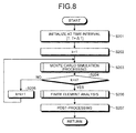
- FIG. 8 is a flowchart illustrating the procedures of the simulation processing in the embodiment.
- the first calculator 15a performs an initialization in the time interval [T, T+ ⁇ T] (S201). For example, the first calculator 15a sets “0" to a variable SumL IR at S201. The first calculator 15a sets "0" to a variable X BD at S201. The first calculator 15a sets “0" to a variable X BD0 at S201. The first calculator 15a sets "1" to a flag flag D0 at S201. The first calculator 15a sets "L s (T)" to a variable L S0 at S201.
- L s (T) is obtained by extracting only a content contributed by a shortening velocity between the filaments from the stretch of the myosin arm 24 at the time T.
- the variable is set to "0" at the processing start time and is updated to an appropriate value after every finite element step is finished, as will be described later.
- FIG. 9 is a view for explaining the example of the calculation method of the stretch of the myosin arm.
- the example of FIG. 9 illustrates the case where the myosin head 22 binds to the actin filament 21 at time tb and the binding is maintained to time T.
- the example of FIG. 9 illustrates the case where the myosin head 22 performs swing motion in the time period from the time tb to the time T.
- the first calculator 15a calculates L s (T) using the following equation (5).
- L T L INIT + L ROT - ⁇ tb T u ⁇ s d s
- L INIT is an initial stretch of the myosin arm 24 at the time of binding.
- L ROT is a stretch due to swing motion of the myosin head 22 after the binding.
- FIG. 8 the first calculator 15a sets a value of a variable k to "1" (S202). Subsequently, the first calculator 15a and the second calculator 15b execute the Monte Carlo simulation processing (S203). The Monte Carlo simulation processing that is executed at S203 is processing at time (T+k ⁇ t).
- FIG. 10 is a flowchart illustrating the procedures of the Monte Carlo simulation processing in the embodiment. As illustrated in FIG. 10 , the first calculator 15a determines whether the state of the myosin head 22 is the binding state (S301).
- the first calculator 15a determines that the myosin head 22 is in the binding state.
- the state of the myosin head 22 is N XB
- the first calculator 15a determines that the myosin head 22 is not in the binding state.
- the first calculator 15a proceeds to S303.
- the first calculator 15a performs various kinds of pre-processing (S302). For example, the first calculator 15a increments the value of the variable X BD by 1 at S302. When the value of the flag flag D0 is "1", the first calculator 15a increments the value of the variable X BD0 by 1 at S302.
- the first calculator 15a calculates the stretch of the myosin arm L at S302, using the following equation (6).
- L : L IR + L S ⁇ 0 - ⁇ ⁇ tX ⁇ B D ⁇ u ⁇ T
- L IR indicates a sum of the above-mentioned L INIT and L ROT .
- L INIT is a stretch of the myosin arm immediately after the transition to the binding state, and is calculated based on the Boltzmann distribution defined from the elastic energy of the myosin arm in consideration of thermal fluctuation, for example.
- the first calculator 15a generates a random number and calculates the state of the myosin head 22 using the generated random number (S303). This enables the first calculator 15a to calculate a stochastic behavior of the myosin head 22.
- the second calculator 15b determines whether the state of the myosin head 22 has transitioned (S304). When the state of the myosin head 22 has not transitioned (No at S304), the second calculator 15b proceeds to S306.
- the second calculator 15b When the state of the myosin head 22 has transitioned (Yes at S304), the second calculator 15b performs state transition processing (S305). For example, when the state of the myosin head 22 has transitioned from the non-binding state N XB to the binding state P XB , the second calculator 15b sets the value of the variable L INIT to the variable L IR and sets the value of the flag flag D0 to "0" at S305.
- the second calculator 15b sets each value of the variable L IR , the variable L S0 , and the variable X Bd to "0" at S305.
- the second calculator 15b performs the following processing at S305.
- the second calculator 15b sets a sum (L IR +X SWING ) of the value of the variable L IR and a length X SWING of the myosin arm 24 extended by the rotation of the myosin head 22 to the variable L IR .
- the second calculator 15b executes post-processing (S306) and stores a processing result in the internal memory. The process then returns. For example, the second calculator 15b sets a sum (SumL IR +L IR ) of the value of the variable SumL IP and the value of the variable L IR to the variable SumL IR at S306. The second calculator 15b sets a sum (SumXB D +XB D ) of the value of the variable SumXB D and the value of the variable XB D to the variable SumXB D .
- the above-mentioned processing is performed by n step times in one step of the finite element analysis.
- the number of consecutive times of the binding state of the myosin head 22 in one step of the finite element analysis is set to the variable SumXB D .
- the sum of L IR in one step of the finite element analysis is set to the variable SumL IR , and these sums are used for calculating an active stress in the finite element analysis, as will be described later.
- the second calculator 15b determines whether the value of the variable k is larger than n (S204). When the value of the variable k is not larger than n (No at S204), the second calculator 15b increments the value of the variable k by 1 (S205), and the process returns to S203. When the value of the variable k is larger than n (Yes at S204), the myocardial model processor 14a executes the finite element analysis (S206).
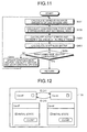
- FIG. 11 is a flowchart illustrating the procedures of the finite element analysis in the embodiment. As illustrated in FIG. 11 , the myocardial model processor 14a calculates various average amounts of one myosin arm (S401).
- the myocardial model processor 14a calculates an average value L AVR of stretch of the myosin arms 24 in one step of the finite element analysis at S401, using the following equation (7).
- L AVR ⁇ ⁇ t ⁇ ⁇ T ⁇ XB D ⁇ 0 ⁇ L S T + SumL IR + ⁇ ⁇ t ⁇ SL 0 2 ⁇ SumXB D ⁇ ⁇ ⁇ ⁇ T + ⁇ ⁇ T
- the myocardial model processor 14a calculates an average value F MH of forces of the myosin arms 24 and an average value K MH of stiffnesses of the myosin arms 24 in one step of the finite element analysis at S401, using the following equation (8).
- F MH dW arm dL L AVR
- K MH d 2 ⁇ W arm dL 2 L AVR
- W arm is the elastic energy of a spring that is given as a function of the stretch L of the myosin arm 24.
- Equation (9) expresses virtual work ⁇ W MH of the myosin arm for a given variation ⁇ of the stretch along the fiber direction.
- ⁇ ⁇ W MH F MH ⁇ SL 0 2 ⁇ ⁇
- the myocardial model processor 14a calculates an active stress S active such that virtual work made by the myocardial models 13a per unit volume and virtual work made by a group of myosin arms in one step of the finite element analysis are equal to each other for any variation ⁇ E of strain on the myocardial continuum model, based on the following equation (10).
- the myocardial model processor 14a calculates a contraction force F of the myocardial model 13a per unit sectional area (S402), using the following equation (11) based on the equation (10).
- F MH im ⁇ is
- the myocardial model processor 14a calculates a stiffness K of the myocardial model 13a per unit sectional area at S402, using the following equation (12).
- K MH im ⁇ SumXB D im ⁇ is
- Equation (13) and (14) each indicate a relation between the variation of the Green-Lagrange strain tensor and the variation of the stretch ⁇ along the fiber direction.
- equation (10) is satisfied by the calculation of the active stress tensor S active as indicated by the following equation (15) using F calculated in the equation (11).
- the myocardial model processor 14a calculates S active using the equation (15) (S403).
- the myocardial model processor 14a calculates a stiffness matrix used in the implicit method (S404), using the following equations (16) and (17).
- the myocardial model processor 14a calculates an equivalent nodal force from the active stress S active calculated by the equation (10) and the stiffness matrix based on the equation (16) and the equation (17), and superimposes them for all the elements to create a right-hand side vector and a coefficient matrix of the linear equation on the Newton-Raphson iteration at S404.
- the Newton-Raphson iteration is finished, a processing result is stored in the internal memory, and the process returns.
- the myocardial model processor 14a solves the linear equation and updates a displacement vector, a velocity vector, and an acceleration vector of the continuum model based on the obtained solution. The process then returns to S401 and shifts to subsequent Newton-Raphson iteration. Note that the initial values of these respective vectors at the time step T+ ⁇ T are assumed to be values of the vectors at the time T.
- the average stretch L AVR of each myosin arm in the time interval [T, T+ ⁇ T] is calculated from the temporal differentiation of the stretch ⁇ along the fiber direction at the time T+ ⁇ T. That is to say, the motion of the continuum model is fed back to the calculation of the contraction force in a strongly coupled manner, so that an influence of the cross-bridge interactions in the time interval [T, T+ ⁇ T] is appropriately reflected to the stiffness matrix. This can provide a stable calculation.
- the myocardial model processor 14a updates the variable Ls for calculation at the next time step (S207), using the following equation (18). This update correctly resets, to Ls, the contribution of the shortening velocity in the stretch L of the myosin arm spring by the time T+ ⁇ T.
- L S ⁇ T + ⁇ ⁇ T : L S ⁇ 0 - ⁇ ⁇ tX ⁇ B D ⁇ u ⁇ ⁇ T + ⁇ ⁇ T
- the receiver 14d receives the definition of the states and the transitions of the T/T units 20 and the definition of the states and the transitions of the myosin head 22 that are defined in the sarcomere models 13b. The receiver 14d then reflects the received contents to each model.
- FIG. 12 to FIG. 18 are views for explaining pieces of information that are received by the receiver in the embodiment.
- the receiver 14d executes the following processing. Specifically, the receiver 14d causes the display unit 12 to display a screen 30 on which the state and the transition of the T/T unit 20 are received.
- FIG. 12 illustrates the case where the two states of "Ca-off” and "Ca-on” are defined through the screen 30.
- Checking a check box next to "Initial State” sets the state corresponding to the checked check box to a state at the start time of the biological simulation processing.
- the example of FIG. 12 indicates that the state at the start time of the biological simulation processing is "Ca-off".
- the receiver 14d executes the following processing. Specifically, the receiver 14d causes the display unit 12 to display a screen 31 on which the state and the transition of the myosin head 22 are received.
- the example of FIG. 13 illustrates the case where four states of "N_XB", "P_XB", "XB_PreR” and "XB-PostR” are defined through the screen 31. Checking a check box next to "Initial State” sets a state corresponding to the checked check box to a state at the start time of the biological simulation processing.
- FIG. 13 illustrates the case where four states of "N_XB", "P_XB", "XB_PreR" and "XB-PostR" are defined through the screen 31. Checking a check box next to "Initial State” sets a state corresponding to the checked check box to a state at the start time of the biological simulation processing.
- FIG. 13 illustrates the case where four states of "N_XB”, "P_XB”, "XB_PreR” and
- the screen 31 illustrated in FIG. 13 indicates that the state at the start time of the biological simulation processing is "N_XB".
- the screen 31 illustrated in FIG. 13 includes radio buttons for setting the respective four states to be "Nobinding (non-binding state)" or "Binding (binding state)".
- the example of FIG. 13 indicates that "N_XB” and “P_XB” are the non-binding state and "XB_PreR” and "XB_PostR” are the binding state.
- the receiver 14d executes the following processing. Specifically, the receiver 14d causes the display unit 12 to display a screen 32 and a screen 33 for defining a function.
- the example of FIG. 14 indicates the case where a state function knp of the T/T unit 20 is defined through the screen 32. With the state function knp, for example, "K_NP0" is returned when the state is "Ca-off", and "K_NP1" is returned when the state is "Ca-on”.
- the example of FIG. 15 indicates the case where a state function ng of the myosin head 22 is defined through the screen 33.
- the receiver 14d causes the display unit 12 to display a screen 34 for defining a transition rate from "N_XB” to "P_XB".
- the example of FIG. 16 illustrates the case where the function knp returning a value in accordance with the state of the T/T unit 20 above the actin section just above the myosin head 22 with get(TT,knp) is used to define the transition rate from "N_XB" toward "P_XB".
- xi_overlap() is a function to which the overlap state of the actin filaments 21 defined from the sarcomere length is reflected, and is a function obtained by multiplying the function ⁇ RA and the function ⁇ LA illustrated in FIG. 6 .
- the receiver 14d when the user operates the input unit 11 to select an arrow from "XB_PreR" toward "XB_PostR”, the receiver 14d performs the following processing. Specifically, the receiver 14d causes the display unit 12 to display a screen 35 for defining a transition rate from "XB_PreR" toward "XB_PostR” that involves the rotation of the myosin head 22. In the example of FIG. 17 , when the transition is a transition involving the rotation of the myosin head 22, the user checks a check box next to "Myosin head swing". Furthermore, in the example of FIG. 17 , the user inputs an increment of the stretch of the myosin arm 24 due to the rotation as X_SWING.
- the stretch L of the myosin arm 24 in the original state "XB_PreR" of the myosin head 22 is called with the function arm_length().
- the elastic energy of the myosin arm 24 with the stretch of the myosin arm, arm_length()+X_SWING, in the state after the transition is obtained with calling spring_energy.
- a transition rate r is defined with a Boltzmann factor defined from a total energy obtained by summing the elastic energy and a chemical energy E_XBPostR in the myosin head 22 after transition.
- the receiver 14d when the user operates the input unit 11 to select an arrow from "XB_PostR" toward "N_XB”, the receiver 14d performs the following processing. Specifically, the receiver 14d causes the display unit 12 to display a screen 36 for defining a transition rate from "XB_PostR" toward "N_XB” that involves dissociation of the myosin head 22.
- FIG. 18 illustrates the case where the user checks check boxes of the "ATP binding" and the "ADP release” in an assumption that ADP dissociates from the myosin head 22 and ATP binds thereto newly for the transition from the binding state to the non-binding state.
- the biological simulation device 10 according to the embodiment can calculate a consumption amount and a generation amount of molecules in the execution of the biological simulation, based on the above-mentioned specification by the user.
- FIG. 19 is a view illustrating a result of automatic generation of the code (Monte Carlo code) for executing the Monte Carlo step based on the definition of the states of the myosin head and the transitions between the states.
- the code firstly generates a random number r in [0, 1], and executes processing in accordance with the current state.
- the variable (XB D and L) of the myosin head 22 is updated with the processing update_XB() as described in step S302 above.
- the code executes one of process_transition_state to process_transition_stateN in accordance with the current state among N states.
- the state is updated with update_stater() in accordance with the value of the random number r, and the variables are updated with update_variables() in accordance with the kind of transition, as described in step S305 above.
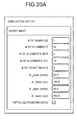
- FIG. 20A and FIG. 20B illustrate examples where the code illustrated in FIG. 19 and the finite element code of the myocardial model 13a are combined as in the processing illustrated in FIG. 8 to execute simulation of heart beat through a coupling analysis with the myocardial model 13a.
- the examples employ a rotationally symmetric continuum obtained by rotating the section illustrated in FIG. 20B as the left ventricle model.
- FIG. 20A illustrates the case where the user specifies the number of elements in the wall penetrating direction and the lengthwise direction with "# of elements in R" and "# of elements in L" through the screen displayed on the display unit 12 by the receiver 14d.
- FIG. 20A illustrates the case where the user specifies the number of beats to be simulated with the "# of heart beats”.
- FIG. 20A illustrates the case where the user specifies the distribution in the fiber direction, as illustrated in FIG. 20B , with " ⁇ _base” and " ⁇ _apex”.
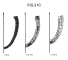
- FIG. 21A to FIG. 21C are views illustrating examples of a simulation result.
- the simulation result illustrated in FIG. 21A includes output of an ejection amount (Ejection) by each beat, a ratio (Ejection Fraction) of the ejection amount and the energy, and a work amount (Muscle Work) made by the myocardial model.
- the simulation result illustrated in FIG. 21A also includes output of a work amount (Ejection work), an ATP consumption amount (ATP consumption), and efficiency (Efficiency) in the ejection of blood.
- the simulation result illustrated in FIG. 21B includes output of a temporal changes of the intraventricular volume and the intraventricular pressure, and temporal changes of conversion results of the work rate and ATP consumption rate, required for the ejection of blood, into hydrolysis energy.
- the simulation result as illustrated in FIG. 21C indicates temporal changes of integrated values of work made by the respective elements in one beat.
- the biological simulation device 10 according to the embodiment can analyze the relation between phenomena at the molecular level in the sarcomere models 13b and the performance of the heart beat.
- the biological simulation device 10 performs the following processing using the sarcomere model 13b that defines a plurality of states of a plurality of actins and a plurality of myosins in the sarcomere contained in the muscle of the biological body and transition rates among a plurality of states. Specifically, the biological simulation device 10 calculates the states of the respective actins and the states of the respective myosins. The biological simulation device 10 calculates the behaviors of the respective actins and the behaviors of the respective myosins based on the respective states of the actins and the respective states of the myosins. Thus, the biological simulation device 10 can calculate the stochastic behaviors of the respective actins and myosins. This enables the biological simulation device 10 to provide an accurate simulation result.
- the biological simulation device 10 calculates the behavior of the sarcomere based on the behaviors of the actins and the behaviors of the myosins, and calculates the behavior of the muscle based on the behaviors of the respective sarcomeres.
- the biological simulation device 10 according to the embodiment can couple the simulation of calculating the behavior of the muscle and the simulation of calculating the behaviors of the sarcomeres.
- the biological simulation device 10 calculates the behaviors of the respective actins and the behaviors of the respective myosins at the intervals ⁇ t.
- the biological simulation device 10 then calculates the behavior of the muscle based on the behaviors of the respective sarcomeres that are calculated in ⁇ T at intervals ⁇ T longer than ⁇ t.
- the biological simulation device 10 calculates the behavior of the muscle using the behaviors of the respective actins and the behaviors of the respective myosins calculated by a plurality of times in ⁇ T.
- the biological simulation device 10 can select the time interval ⁇ T, at which the behavior of the muscle is calculated, in accordance with the convenience of the finite element analysis and can execute the phenomenon at the order of seconds, such as the heart beat, at an appropriate time. Even with such a gap of the time intervals, a coupling analysis with high accuracy can be performed because work amounts on the sarcomere models and the myocardial model are matched as illustrated in the equation (10). Furthermore, as indicated by the equation (7), the average stretch L AVR of the myosin arm in the time interval [T,T+ ⁇ T] is calculated from the stretch velocity at the time T+ ⁇ T.
- the sarcomere model 13b on which the biological simulation device 10 according to the embodiment performs processing, is defined such that when a myosin binding to an actin increases a probability that another myosin in a particular range from the myosin binds to the actin. Furthermore, the state transitions of each myosin head are defined in accordance with the overlap state of the actin filaments just above the myosin head. That is to say, the sarcomere model 13b is defined so as to indicate a behavior similar to that of a real sarcomere.
- the simulation device 10 calculates the states of the respective actins and the states of the respective myosins, using the sarcomere model 13b. As a result, the simulation device 10 can calculate the state similar to that of the real sarcomere.
- the biological simulation device 10 calculates the length of the stretch of the myosin based on the length of the stretch of the myosin arm due to the binding of the myosin to the actin, the length of the stretch of the myosin arm due to the rotation of the myosin head, and an integrated value of the shortening velocity of the myosin.
- the biological simulation device 10 receives a plurality of states of a plurality of actins, transitions between the states of the actins, a plurality of states of a plurality of myosins, and transitions between the states of the myosins, which are defined for the sarcomere model 13b.
- the biological simulation device 10 generates the Monte Carlo code for executing the Monte Carlo step based on the received contents. This enables even a user such as a researcher who studies hearts medically but is not good at programming to perform a simulation of any desired sarcomere model without performing programming.
- the device of the invention may be executed in various different modes other than the above-mentioned embodiment.
- the entire processing or a part of the processing described in the above-mentioned embodiment that is performed automatically may be performed manually.
- the entire processing or a part of the processing described in the above-mentioned embodiment that is performed manually can be performed automatically with a known method.
- processing at the steps in the processes described in the above-mentioned embodiment can be subdivided into small pieces or be compiled as appropriate depending on various loads or usage conditions. Alternatively, any of the steps can be omitted.
- FIG. 22 is a diagram illustrating the computer that executes a biological simulation program.
- a computer 300 includes a plurality of multi-core CPUs 310, a ROM 320, a hard disk drive (HDD) 330, and a RAM 340.
- Each CPU 310 includes cores 310a's. These components 310 to 340 are connected to one another via a bus 350.
- the ROM 320 stores therein a basic program such as an OS.
- the HDD 330 previously stores therein a biological simulation program 330a exhibiting the same functions as those of the myocardial model processors 14a, the sarcomere model processors 14b, the first calculators 15a, and the second calculators 15b in the above-mentioned first embodiment. Note that the biological simulation program 330a may be separated as appropriate.
- the CPUs 310 load the biological simulation program 330a from the HDD 330 and execute it.
- the above-mentioned biological simulation program 330a is not necessarily stored in the HDD 330 initially.
- the computer 300 may load the biological simulation program 330a from the biological simulation program 330a stored in a "mobile physical medium” such as a flexible disk (FD), a compact disk read only memory (CD-ROM), a digital versatile disk (DVD), a magnetooptical disk, and an IC card that is inserted into the computer 300, and execute it.
- a "mobile physical medium” such as a flexible disk (FD), a compact disk read only memory (CD-ROM), a digital versatile disk (DVD), a magnetooptical disk, and an IC card that is inserted into the computer 300, and execute it.
- the computer 300 may load the biological simulation program 330a from the biological simulation program 330a stored in "another computer (or server)" that is connected to the computer 300 through a public line, the Internet, a LAN, a wide area network (WAN), or the like, and execute it.
- another computer or server
- an accurate coupling simulation result of molecular models having stochastic behaviors and motion of muscle as a continuum can be obtained.
Landscapes
- Physics & Mathematics (AREA)
- Health & Medical Sciences (AREA)
- Life Sciences & Earth Sciences (AREA)
- Engineering & Computer Science (AREA)
- Bioinformatics & Cheminformatics (AREA)
- Biophysics (AREA)
- Molecular Biology (AREA)
- Physiology (AREA)
- Bioinformatics & Computational Biology (AREA)
- Biotechnology (AREA)
- Evolutionary Biology (AREA)
- General Health & Medical Sciences (AREA)
- Medical Informatics (AREA)
- Spectroscopy & Molecular Physics (AREA)
- Theoretical Computer Science (AREA)
- Management, Administration, Business Operations System, And Electronic Commerce (AREA)
- Measuring And Recording Apparatus For Diagnosis (AREA)
Abstract
Description
- The embodiments discussed herein are related to a biological simulation program, a biological simulation method, and a biological simulation device.
- In the field of molecular biology, diverse sarcomere models have been proposed that describe cross-bridge interactions between myosins and actins in sarcomeres based on experimental facts. One exemplary sarcomere model defines a plurality of representative states of molecules contributing to the binding between the myosin and the actin in the sarcomere and defines the transition rate between these states in consideration of interactions among the neighboring molecules, energy of the molecules, and the like. Generally, in a coupling analysis of the molecular motions in sarcomeres and the muscular continuum model, an ordinary differential equation is derived where a state concentration is set as a variable based on the average behavior of the molecular models. Usually, a contraction force on the continuum model is calculated based on calculation results of the sarcomere models and motion of muscle as the continuum is calculated based on the result.
- Various researches have been made as can be seen in: Peterson J.N., Hunter W.C., Berman M.R.: Estimated time course of Ca2+bound to troponin C during relaxation in isolated cardiac muscle, American Physiological Society, H1013-H1024(1991); Hunter P.J., McCulloch A.D., ter Keurs H.E.D.J.: Modeling the mechanical properties of cardiac muscle, Progress in Biophysics & Molecular Biology 69, 289-331(1998); Razumova M.V., Bukatina A.E., Campbell K.B.: Stiffness-distortion sarcomere model for muscle simulation. J. Appl. Physiol. 87, 1861-1876(1999); Rice J.J., Wang F., Bers D.M., de Tombe P.P.: Approximate model of cooperative activation and crossbridge cycling in cardiac muscle using ordinary differential equations. Biophys. J. 95, 2368-2390(2008).
- The above-mentioned sarcomere models indicate an averaged behavior of the molecular models in the sarcomere models. The simulation of behaviors of sarcomeres using these sarcomere models, therefore, provides simulation results lacking accuracy with respect to the state transitions of the molecular models. This results in a problem that a simulation result for motion of a muscle as the continuum also lacks accuracy. Furthermore, the muscular motion is strongly fed back to the state transitions of the molecules in the sarcomere model. For this reason, it is difficult to execute a reliable analysis by the simulation based on one-way information transmission from the sarcomere models to the continuum model.
- Accordingly, it is an object in one aspect of an embodiment of the invention to provide an accurate result of a coupling simulation of molecular models having stochastic behaviors and a motion of muscle as a continuum. It is an object in another aspect of an embodiment of the invention to perform a coupling analysis stably in an appropriate time step through taking a feedback of the motion of the muscular continuum model to the molecular models into the coupling simulation based on an implicit solution.
- According to an aspect of an embodiment, a biological simulation method and a biological simulation program causes a computer to execute a following process. Firstly, calculating states of a plurality of actins and states of a plurality of myosins in a sarcomere contained in a muscle of a biological body using a model that defines a plurality of states of the actins and a plurality of states of the myosins and transition rates between the states. Secondly, calculating behaviors of the respective actins and behaviors of the respective myosins based on the states of the actins and the states of the myosins, respectively. Thirdly, calculating a behavior of the sarcomere based on the behaviors of the actins and the behaviors of the myosins. Fourthly, calculating a behavior of the muscle based on the behavior of the sarcomere.
- According to another aspect of an embodiment, a biological simulation device includes a first calculator, a second calculator, and a third calculator. The first calculator is configured to calculate states of a plurality of actins and states of a plurality of myosins in a sarcomere contained in a muscle of a biological body using a model that defines a plurality of states of the actins and a plurality of states of the myosins and transition rates between the states. The second calculator is configured to calculate behaviors of the respective actins and behaviors of the respective myosins based on the states of the actins and the states of the myosins, respectively. The third calculator is configured to calculate a behavior of the sarcomere based on the behaviors of the actins and the behaviors of the myosins and calculate a behavior of the muscle based on the behavior of the sarcomere.
-
-
FIG. 1 is a diagram illustrating an example of a functional configuration of a biological simulation device according to an embodiment; -
FIG. 2 is a view illustrating a part of an example of a myocardial model; -
FIG. 3 is a view illustrating an example of a sarcomere model; -
FIG. 4 is a view illustrating an example of a state transition of a T/T unit; -
FIG. 5 is a view illustrating an example of a state transition of a myosin head; -
FIG. 6 is a view for explaining a change of an overlap state of actin filaments in accordance with sarcomere length (SL); -
FIG. 7 is a flowchart illustrating procedures of biological simulation processing in the embodiment; -
FIG. 8 is a flowchart illustrating procedures of simulation processing in the embodiment; -
FIG. 9 is a view for explaining an example of a calculation method of a stretch of a myosin arm; -
FIG. 10 is a flowchart illustrating procedures of Monte Carlo simulation processing in the embodiment; -
FIG. 11 is a flowchart illustrating procedures of a finite element analysis in the embodiment; -
FIG. 12 is a view for explaining transition information of the T/T unit that is received by a receiver in the embodiment; -
FIG. 13 is a view for explaining information of the myosin head that is received by the receiver in the embodiment; -
FIG. 14 is a view for explaining function information that relates to a state of the T/T unit and is received by the receiver in the embodiment; -
FIG. 15 is a view for explaining function information that relates to a state of the myosin head and is received by the receiver in the embodiment; -
FIG. 16 is a view for explaining information that defines a transition between a non-binding state and a binding state of the myosin head and is received by the receiver in the embodiment; -
FIG. 17 is a view for explaining information that defines a transition between states before and after swing of the myosin head and is received by the receiver in the embodiment; -
FIG. 18 is a view for explaining information that defines transition between binding and dissociation that is received by the receiver in the embodiment; -
FIG. 19 is a view illustrating a result of automatic generation of a code (Monte Carlo code) for executing a Monte Carlo step based on the definition of states of the myosin head and state transitions; -
FIG. 20A is a view illustrating an example of parameter specification relating to a myocardial continuum model when simulation of heart beat is executed; -
FIG. 20B is a view illustrating an example of a method of specifying the fiber direction when the simulation of the heart beat is executed; -
FIG. 21A is a table illustrating an example of a simulation result of various amounts relating to performance of the heart beat; -
FIG. 21B is a graph illustrating an example of simulation results of left ventricle pressure-volume change (upper graph) and work rate and energy consumption rate (lower graph); -
FIG. 21C is a view illustrating an example of a simulation result relating to distribution of a contraction force; and -
FIG. 22 is a diagram illustrating a computer that executes a biological simulation program. - Preferred embodiments of the present invention will be explained with reference to accompanying drawings. Note that the embodiments do not limit disclosed techniques.
- The following describes the biological simulation device according to an embodiment. The biological simulation device in the embodiment performs the following processing using a model that defines a plurality of states of a plurality of actins and a plurality of myosins in a sarcomere contained in a muscle of a biological body and transition rates between the states, and a muscular continuum model expressed in a finite element mesh. That is to say, the biological simulation device calculates state transitions of the actins and the myosins that are embedded in finite elements of the muscular continuum model. The biological simulation device solves an equation of motion with which contraction forces generated by respective molecules, which are derived from state transitions of the molecular models and motion of the muscle as a continuum, are matched with a contraction force of the continuum model of the finite elements into which molecular models are embedded to perform the following analysis. That is, the biological simulation device performs an analysis that couples the molecular state transition motion and the muscular motion.
FIG. 1 is a diagram illustrating a functional configuration of the biological simulation device according to the embodiment. As illustrated inFIG. 1 , thisbiological simulation device 10 includes aninput unit 11, adisplay unit 12, astorage unit 13, and acontroller 14. - The
input unit 11 inputs various kinds of information to thecontroller 14. For example, upon receiving an instruction to execute biological simulation processing, which will be described later, from a user, theinput unit 11 inputs the received instruction to thecontroller 14. Examples of a device as theinput unit 11 includes a keyboard and a mouse. - The
display unit 12 displays various kinds of information. For example, thedisplay unit 12 displays a simulation result under control by adisplay controller 14c, which will be described later. - The
storage unit 13 stores therein various types of programs that are executed by thecontroller 14. Thestorage unit 13 stores thereinmyocardial models 13a andsarcomere models 13b. - The
myocardial models 13a are models obtained by dividing a muscular model of the entire heart as a continuum into a plurality of elements. For example, the muscular model of the entire heart is divided into four models of the left atrium, the left ventricle, the right atrium, and the right ventricle, and each of the left atrium model, the left ventricle model, the right atrium model, and the right ventricle model can be set as themyocardial model 13a. Themyocardial model 13a is used to calculate a behavior of a muscular model indicated by themyocardial model 13a in the finite element analysis.FIG. 2 is a view illustrating a part of an example of the myocardial model. In the example ofFIG. 2 , themyocardial model 13a is the left ventricle model, and a part of the left ventricle model is illustrated. The example ofFIG. 2 illustrates the fiber directions of a plurality of elements 13a_1 in the finite element mesh of themyocardial model 13a with arrows. In the following description, a vector of the fiber direction is expressed with f in some cases. - Each of the elements 13a_1 includes a plurality of
sarcomere models 13b embedded therein. The following describes the case where the element 13a_1 includes "ns"sarcomere models 13b embedded therein. Each of thesarcomere models 13b is a model in which molecules as components indicate stochastic behaviors. Thesarcomere model 13b is defined so as to have so-called cooperativity and so-called sarcomere length dependency.FIG. 3 is a view illustrating an example of the sarcomere model. As illustrated inFIG. 3 , thesarcomere model 13b includes a plurality of T/T units (troponin/tropomyosin units) 20 on anactin filament 21 and a plurality of myosin heads 22 on amyosin filament 23. As will be described later, thesarcomere model 13b also includesmyosin arms 24 connecting themyosin filament 23 and the myosin heads 22 (seeFIG. 5 ). The following describes the case where onesarcomere model 13b includes "nm" pairs of the myosin heads 22 and themyosin arms 24. - The
sarcomere model 13b defines a plurality of states for the T/T unit 20 and themyosin head 22, and Monte Carlo simulation is executed in accordance with the previously defined transition rates among the states. That is to say, the stochastic behaviors of the T/T unit 20 and themyosin head 22 are calculated through the Monte Carlo simulation. - The state transition rates of the T/
T unit 20 are controlled in accordance with the states of themyosin head 22 just under the T/T unit 20.FIG. 4 is a view illustrating an example of a state transition of the T/T unit. As illustrated inFIG. 4 , the embodiment includes two types of states including a state (binding state: Ca-on) where calcium ion (Ca2+) binds to the T/T unit 20 and a state (non-binding state: Ca-off) where no calcium ion (Ca2+) binds to the T/T unit 20. In the state transition illustrated inFIG. 4 , for example, the state is more likely to transition to the binding state as the concentration of the calcium ion is higher. Furthermore, a dissociation probability Koff of the calcium ion is defined in accordance with the state of themyosin head 22 just under the T/T unit 20. Furthermore, values of Kon and Koff change depending on whether themyosin head 22 binds to the actin section under the corresponding T/T unit 20. For example, Koff has a small value when themyosin head 22 binds to the actin section under the T/T unit 20, and the calcium ion is less likely to dissociate from the T/T unit 20. That is to say, the T/T unit 20 in thesarcomere model 13b in the embodiment is a model having cooperativity in which the calcium ion is less likely to dissociate from the T/T unit 20 when themyosin head 22 binds to the actin section under the T/T unit 20. The binding of the calcium ion binds to the T/T unit 20 shifts the position of tropomyosin, which is a string-like protein hiding a binding site to themyosin head 22, and this facilitates the binding of themyosin head 22 to the actin section under the T/T unit 20. Thus, the binding of the calcium ion to the T/T unit 20 increases the probability that themyosin head 22 binds to the actin section under the T/T unit 20. The binding of themyosin head 22 to the actin section under the T/T unit 20 further shifts the position of the tropomyosin, and this increases the probability that aneighbor myosin head 22 neighboring the myosin binds to the actin section just above themyosin head 22. The actin section under the T/T unit 20 indicates a section partitioned by lines indicated by thereference numeral 20 inFIG. 3 , and theneighbor myosin head 22 indicates amyosin head 22 in a particular range from onemyosin head 22. - The state transition of the
myosin head 22 is controlled in accordance with states of theneighbor myosin head 22 and the T/T unit 20 on the actin section just above themyosin head 22.FIG. 5 illustrates an example of the state transition of the myosin head. As illustrated inFIG. 5 , the embodiment includes four kinds of states of NXB, PXB, XBPreR, and XBPostR. NXB is a state (non-binding state) where themyosin head 22 does not bind to the actin section under the T/T unit 20. PXB is a state (weak-binding state) where themyosin head 22 starts binding to the actin section under the T/T unit 20. XBPreR is a state (strong-binding state (1)) where the chemical state of themyosin head 22 changes from that in PXB and themyosin head 22 binds to the actin section under the T/T unit 20 more strongly. XBPostR is a state (strong-binding state (2)) where themyosin head 22 keeps binding to the actin section controlled by the T/T unit 20 and a rotating motion (swing motion) of themyosin head 22 is generated from XBPreR. InFIG. 5 , knp is a coefficient in the transition from NXB to PXB. As an overlap of theactin filaments 21 in thesarcomere model 13b is larger, a range of the actin filament to which the myosin heads 22 can bind is shorter. That is, as the overlap of theactin filaments 21 in thesarcomere model 13b is larger, the myosin heads 22 are less likely to bind to the actin. In the embodiment, the value of knp is smaller as the overlap of theactin filaments 21 in thesarcomere model 13b is larger, which decreases the probability that the myosin heads 22 bind to the actin. - kpn is a coefficient in the transition from PXB, XBPreR, or XBPostR to NXB. In addition, γn and γ-n indicate cooperativity relating to the transition between the non-binding state and the binding state of the
myosin head 22. The numeral n indicates the number (0 to 2) of neighboring myosin heads 22 that bind to the actin. For example, in the case of γ=80 and the number of the neighboring myosin heads 22 that bind to the actin is "1", γn is "80". That is to say, in the case illustrated inFIG. 5 , themyosin head 22 is 80 times more likely to bind to the actin. In the case of γ=80 and the number of the neighboring myosin heads 22 that bind to the actin is "2", γn is "6400". That is to say, in the case illustrated inFIG. 5 , themyosin head 22 is 6400 times more likely to bind to the actin. In the case of γ=80 and the number of the neighboring myosin heads 22 that bind to the actin is "1", γ-n is "1/80". That is to say, in the case illustrated inFIG. 5 , themyosin head 22 is 1/80 times more likely to dissociate from the actin. In the case of γ=80 and the number of the neighboring myosin heads 22 that bind to the actin is "2", γ-n is 1/6400. That is to say, in the case illustrated inFIG. 5 , themyosin head 22 is 1/6400 times more likely to dissociate from the actin. Thus, themyosin head 22 that does not bind to the actin is more likely to bind to the actin when the neighboringmyosin head 22 binds to the actin. Furthermore, themyosin head 22 that binds to the actin is less likely to dissociate from the actin when the neighboringmyosin head 22 also binds to the actin. - In
FIG. 5 , adenosine triphosphate (ATP) binds to themyosin head 22 in the state of NXB, PXB, or XBPreR. A hydrolysis reaction from ATP to adenosine diphosphate (ADP) + phosphoric acid (pi) generates energy. - In
FIG. 5 , fapp is defined such that the state distribution is an equilibrium state based on the Boltzmann distribution law through the transition from PXB to XBPreR. In addition, gapp is defined such that the state distribution is an equilibrium state based on the Boltzmann distribution law through the transition from XBPreR to PXB. - In the transition from XBPreR to XBPostR and the transition from XBPostR to XBPreR, the
myosin head 22 performs swing motion. InFIG. 5 , hf and hb are defined such that the state distribution is an equilibrium state, based on the Boltzmann distribution law, that is defined from a sum of a chemical energy in the myosin head and the elastic energy of the myosin arm through a change of the length of the myosin arm with the swing motion of themyosin head 22. Furthermore, gxb inFIG. 5 is a transition rate that indicates ease of dissociation from XBPostR other than the above-mentioned effects of the cooperativity. InFIG. 5 , α is a coefficient of equal to or lower than 1 that indicates resistance to dissociation of themyosin head 22 from the actin in the strong-binding states XBPreR and XBPostR. - The following describes a change of the overlap state of the
actin filaments 21 in accordance with the sarcomere length (SL). First, the SL can be calculated through the following method. That is to say, a stretch along the fiber direction λ(T) is calculated for each of the elements 13a_1 in themyocardial model 13a at time T, using the following equation (1).
Note that F(T) is a deformation gradient tensor of themyocardial model 13a at the time T. - Subsequently, the velocity (stretch velocity) along the fiber direction


- The sarcomere length SL(T) of the
sarcomere model 13b at the time T is calculated, using the following equation (3).
Note that SL0 is a sarcomere length in a no-load state when the time T is 0. - Subsequently, a shortening velocity

sarcomere model 13b is calculated, using the following equation (4).
- The following describes a change of the overlap state of the
actin filaments 21 in accordance with the sarcomere length (SL) with reference toFIG. 6. FIG. 6 is a view for explaining the change of the overlap state of theactin filaments 21 in accordance with the SL. The example ofFIG. 6 illustrates sarcomere lengths SL(T1), SL(T2), and SL(T3) at times T1, T2, and T3, respectively. As illustrated in the upper example inFIG. 6 , when the sarcomere length (SL) is too large, there is no actin to which a myosin head at the center region can bind. As illustrated in the lower example inFIG. 6 , when the sarcomere length (SL) is too small, an overlapping portion of theactin filaments 21 is formed in the vicinity of the center, and it is difficult for a myosin head located in this portion to bind to the actin. In consideration of the above, in the embodiment, functions χLA and χRB can be configured for reflecting the overlap state of the actin filaments to the state transition of themyosin head 22, and transition rates in the respective state transitions of themyosin head 22 to the binding state can be determined with reference to the functions χLA and χRB. - In the embodiment, unlike the conventional model using the ordinary differential equation, an average behavior is not described using one representative unit. The state transitions of the respective T/
T units 20 and the respective myosin heads 22 are controlled also with reference to the neighbor states. For this reason, according to the embodiment, the state transitions of the micro models are simulated in a manner closer to the reality while preventing errors due to averaging or the like. This makes it possible to perform an accurate coupling analysis with the myocardial continuum model, as will be described below. - The
storage unit 13 is a storage device exemplified by a semiconductor memory element such as a flash memory, a hard disk, and an optical disk. Note that thestorage unit 13 is not limited to the above-mentioned kinds of storage devices and may be a random access memory (RAM), a read only memory (ROM), or the like. - The
controller 14 includes an internal memory for storing programs defining various processing procedures and control data, and executes various kinds of processing by the use of them. As illustrated inFIG. 1 , thecontroller 14 includes a plurality ofmyocardial model processors 14a, a plurality ofsarcomere model processors 14b, adisplay controller 14c, and areceiver 14d. - The
myocardial model processors 14a correspond to the respective elements in themyocardial model 13a, and each of themyocardial model processors 14a calculates the behavior of the correspondingmyocardial model 13a. Thesarcomere model processors 14b correspond to therespective sarcomere models 13b, and each of thesarcomere model processors 14b calculates the behavior of thecorresponding sarcomere model 13b. Thecontroller 14 includes one or a plurality of multi-core central processing unit(s) (CPU(s)) having a plurality of cores as operation processors. Alternatively, thecontroller 14 may include a plurality of single-core CPUs having one core as the operation processor. The cores each execute a biological simulation program described later, thereby implementing each part of themyocardial model processors 14a, thesarcomere model processors 14b, thedisplay controller 14c, and thereceiver 14d. - Each of the
sarcomere model processors 14b includes afirst calculator 15a and asecond calculator 15b. - The following describes an example of processing that is executed by the
controller 14 with reference toFIG. 7. FIG. 7 is a flowchart illustrating procedures of the biological simulation processing in the embodiment. The biological simulation processing is executed when theinput unit 11 inputs an instruction to execute the biological simulation processing to thecontroller 14, for example. In the biological simulation processing, the finite element analysis of themyocardial models 13a is executed in time intervals ΔT. Furthermore, in the Monte Carlo simulation processing on the sarcomere models, simulation on thesarcomere models 13b with the Monte Carlo method is executed at time steps Δt (ΔT / n) obtained by dividing the time interval [T, T+ΔT] into small time segments of n steps. As the value of ΔT, 2.5 milliseconds can be employed, for example. Alternatively, as the value of Δt, 5 microseconds can be employed, for example. In the Monte Carlo method, a product of a transition rate and the time segment Δt is required not to be larger than 1, so that the above-mentioned small time segments is set. Although it is preferable that the calculation in the finite element analysis be also performed at small time segments in a viewpoint of the accuracy, the above-mentioned time segment ΔT is appropriate therefore because it takes time to solve the linear equation through the implicit method. - As illustrated in
FIG. 7 , themyocardial model processor 14a and thesarcomere model processor 14b execute the simulation processing (S101). After the simulation processing (S101), thecontroller 14 determines whether the time step t in which the simulation processing is performed is the final time step or not (S102). When thecontroller 14 determines that the time step t is not the final time step, thecontroller 14 adds one to t (S103) and the process returns to step S101. On the other hand, when thecontroller 14 determines that the time step t is the final time step, thedisplay controller 14c performs control to display simulation result on the display unit 12 (S104). -
FIG. 8 is a flowchart illustrating the procedures of the simulation processing in the embodiment. As illustrated inFIG. 8 , thefirst calculator 15a performs an initialization in the time interval [T, T+ΔT] (S201). For example, thefirst calculator 15a sets "0" to a variable SumLIR at S201. Thefirst calculator 15a sets "0" to a variable XBD at S201. Thefirst calculator 15a sets "0" to a variable XBD0 at S201. Thefirst calculator 15a sets "1" to a flag flagD0 at S201. Thefirst calculator 15a sets "Ls (T)" to a variable LS0 at S201. Note that Ls (T) is obtained by extracting only a content contributed by a shortening velocity between the filaments from the stretch of themyosin arm 24 at the time T. The variable is set to "0" at the processing start time and is updated to an appropriate value after every finite element step is finished, as will be described later. - The following describes an example of a calculation method of the stretch of the
myosin arm 24 with reference toFIG. 9. FIG. 9 is a view for explaining the example of the calculation method of the stretch of the myosin arm. The example ofFIG. 9 illustrates the case where themyosin head 22 binds to theactin filament 21 at time tb and the binding is maintained to time T. Furthermore, the example ofFIG. 9 illustrates the case where themyosin head 22 performs swing motion in the time period from the time tb to the time T. In the case of the example ofFIG. 9 , thefirst calculator 15a calculates Ls (T) using the following equation (5).
Note that LINIT is an initial stretch of themyosin arm 24 at the time of binding. LROT is a stretch due to swing motion of themyosin head 22 after the binding. - In
FIG. 8 , thefirst calculator 15a sets a value of a variable k to "1" (S202). Subsequently, thefirst calculator 15a and thesecond calculator 15b execute the Monte Carlo simulation processing (S203). The Monte Carlo simulation processing that is executed at S203 is processing at time (T+kΔt).FIG. 10 is a flowchart illustrating the procedures of the Monte Carlo simulation processing in the embodiment. As illustrated inFIG. 10 , thefirst calculator 15a determines whether the state of themyosin head 22 is the binding state (S301). For example, at S301, when the state of themyosin head 22 is any one of PXB, XBPreR, and XBPostR, thefirst calculator 15a determines that themyosin head 22 is in the binding state. When the state of themyosin head 22 is NXB, thefirst calculator 15a determines that themyosin head 22 is not in the binding state. - When the
myosin head 22 is not in the binding state (No at S301), thefirst calculator 15a proceeds to S303. When themyosin head 22 is in the binding state (Yes at S301), thefirst calculator 15a performs various kinds of pre-processing (S302). For example, thefirst calculator 15a increments the value of the variable XBD by 1 at S302. When the value of the flag flagD0 is "1", thefirst calculator 15a increments the value of the variable XBD0 by 1 at S302. In addition, thefirst calculator 15a calculates the stretch of the myosin arm L at S302, using the following equation (6).
Note that LIR indicates a sum of the above-mentioned LINIT and LROT. LINIT is a stretch of the myosin arm immediately after the transition to the binding state, and is calculated based on the Boltzmann distribution defined from the elastic energy of the myosin arm in consideration of thermal fluctuation, for example. - The
first calculator 15a generates a random number and calculates the state of themyosin head 22 using the generated random number (S303). This enables thefirst calculator 15a to calculate a stochastic behavior of themyosin head 22. - Thereafter, the
second calculator 15b determines whether the state of themyosin head 22 has transitioned (S304). When the state of themyosin head 22 has not transitioned (No at S304), thesecond calculator 15b proceeds to S306. - When the state of the
myosin head 22 has transitioned (Yes at S304), thesecond calculator 15b performs state transition processing (S305). For example, when the state of themyosin head 22 has transitioned from the non-binding state NXB to the binding state PXB, thesecond calculator 15b sets the value of the variable LINIT to the variable LIR and sets the value of the flag flagD0 to "0" at S305. When the state of themyosin head 22 has transitioned from any one of the binding states PXB, XBPreR, and XBPostR to the non-binding state NXB, thesecond calculator 15b sets each value of the variable LIR, the variable LS0, and the variable XBd to "0" at S305. When themyosin head 22 remains in any one of the binding states PXB, XBPreR, and XBPostR and performs the swing motion to rotate, thesecond calculator 15b performs the following processing at S305. Specifically, thesecond calculator 15b sets a sum (LIR+XSWING) of the value of the variable LIR and a length XSWING of themyosin arm 24 extended by the rotation of themyosin head 22 to the variable LIR. - The
second calculator 15b executes post-processing (S306) and stores a processing result in the internal memory. The process then returns. For example, thesecond calculator 15b sets a sum (SumLIR+LIR) of the value of the variable SumLIP and the value of the variable LIR to the variable SumLIR at S306. Thesecond calculator 15b sets a sum (SumXBD+XBD) of the value of the variable SumXBD and the value of the variable XBD to the variable SumXBD. The above-mentioned processing is performed by n step times in one step of the finite element analysis. Consequently, the number of consecutive times of the binding state of themyosin head 22 in one step of the finite element analysis is set to the variable SumXBD. Furthermore, the sum of LIR in one step of the finite element analysis is set to the variable SumLIR, and these sums are used for calculating an active stress in the finite element analysis, as will be described later. - In
FIG. 8 , thesecond calculator 15b determines whether the value of the variable k is larger than n (S204). When the value of the variable k is not larger than n (No at S204), thesecond calculator 15b increments the value of the variable k by 1 (S205), and the process returns to S203. When the value of the variable k is larger than n (Yes at S204), themyocardial model processor 14a executes the finite element analysis (S206).FIG. 11 is a flowchart illustrating the procedures of the finite element analysis in the embodiment. As illustrated inFIG. 11 , themyocardial model processor 14a calculates various average amounts of one myosin arm (S401). For example, themyocardial model processor 14a calculates an average value LAVR of stretch of themyosin arms 24 in one step of the finite element analysis at S401, using the following equation (7).
- The
myocardial model processor 14a calculates an average value FMH of forces of themyosin arms 24 and an average value KMH of stiffnesses of themyosin arms 24 in one step of the finite element analysis at S401, using the following equation (8).
Note that Warm is the elastic energy of a spring that is given as a function of the stretch L of themyosin arm 24. - The following equation (9) expresses virtual work δWMH of the myosin arm for a given variation δλ of the stretch along the fiber direction.

- The
myocardial model processor 14a calculates an active stress Sactive such that virtual work made by themyocardial models 13a per unit volume and virtual work made by a group of myosin arms in one step of the finite element analysis are equal to each other for any variation δE of strain on the myocardial continuum model, based on the following equation (10). The following describes an example of the method.
- In the equation (10), "im" indicates the index of the myosin heads 22 on the
myosin filament 23, and "is" indicates the index of thesarcomere models 13b in the element 13a_1. In addition, RSA indicates a proportion of the sarcomeres in the muscle, and SA0 indicates a sectional area of onesarcomere model 13b. Sactive indicates an active stress tensor of the continuum model, δE indicates a variation of a Green-Lagrange strain tensor, and a product of the two tensors indicates virtual work of the continuum. - The
myocardial model processor 14a calculates a contraction force F of themyocardial model 13a per unit sectional area (S402), using the following equation (11) based on the equation (10).
- The
myocardial model processor 14a calculates a stiffness K of themyocardial model 13a per unit sectional area at S402, using the following equation (12).
- The following equations (13) and (14) each indicate a relation between the variation of the Green-Lagrange strain tensor and the variation of the stretch λ along the fiber direction. In consideration of the equation (13), it is known that the equation (10) is satisfied by the calculation of the active stress tensor Sactive as indicated by the following equation (15) using F calculated in the equation (11).


- Thus, the
myocardial model processor 14a calculates Sactive using the equation (15) (S403). When the finite element analysis is executed with an implicit method such as the Newmark-β method, themyocardial model processor 14a calculates a stiffness matrix used in the implicit method (S404), using the following equations (16) and (17).

- These equations are derived from the relational equations (13) and (14) for the stretch λ along the fiber direction and the temporal differentiation thereof and the Green-Lagrange strain tensor E and the temporal differentiation thereof. The
myocardial model processor 14a calculates an equivalent nodal force from the active stress Sactive calculated by the equation (10) and the stiffness matrix based on the equation (16) and the equation (17), and superimposes them for all the elements to create a right-hand side vector and a coefficient matrix of the linear equation on the Newton-Raphson iteration at S404. When the right-hand side vector corresponding to a residual vector is sufficiently small (Yes at S405), the Newton-Raphson iteration is finished, a processing result is stored in the internal memory, and the process returns. When the right-hand side vector corresponding to the residual vector is not sufficiently small (No at S405), themyocardial model processor 14a solves the linear equation and updates a displacement vector, a velocity vector, and an acceleration vector of the continuum model based on the obtained solution. The process then returns to S401 and shifts to subsequent Newton-Raphson iteration. Note that the initial values of these respective vectors at the time step T+ΔT are assumed to be values of the vectors at the time T. As in the equation (7), the average stretch LAVR of each myosin arm in the time interval [T, T+ΔT] is calculated from the temporal differentiation of the stretch λ along the fiber direction at the time T+ΔT. That is to say, the motion of the continuum model is fed back to the calculation of the contraction force in a strongly coupled manner, so that an influence of the cross-bridge interactions in the time interval [T, T+ΔT] is appropriately reflected to the stiffness matrix. This can provide a stable calculation. - When the Newton-Raphson iteration is converged, the finite element analysis is finished. Turning back to
FIG. 8 , themyocardial model processor 14a updates the variable Ls for calculation at the next time step (S207), using the following equation (18). This update correctly resets, to Ls, the contribution of the shortening velocity in the stretch L of the myosin arm spring by the time T+ΔT.
- The
receiver 14d receives the definition of the states and the transitions of the T/T units 20 and the definition of the states and the transitions of themyosin head 22 that are defined in thesarcomere models 13b. Thereceiver 14d then reflects the received contents to each model.FIG. 12 to FIG. 18 are views for explaining pieces of information that are received by the receiver in the embodiment. As illustrated inFIG. 12 , when a user, such as a researcher studying the heart medically, inputs an instruction to display a screen on which the state and the transition of the T/T unit 20 are received through theinput unit 11, thereceiver 14d executes the following processing. Specifically, thereceiver 14d causes thedisplay unit 12 to display ascreen 30 on which the state and the transition of the T/T unit 20 are received. The example ofFIG. 12 illustrates the case where the two states of "Ca-off" and "Ca-on" are defined through thescreen 30. Checking a check box next to "Initial State" sets the state corresponding to the checked check box to a state at the start time of the biological simulation processing. The example ofFIG. 12 indicates that the state at the start time of the biological simulation processing is "Ca-off". - As illustrated in
FIG. 13 , when the user inputs an instruction to display a screen on which the state and the transition of themyosin head 22 are received through theinput unit 11, thereceiver 14d executes the following processing. Specifically, thereceiver 14d causes thedisplay unit 12 to display ascreen 31 on which the state and the transition of themyosin head 22 are received. The example ofFIG. 13 illustrates the case where four states of "N_XB", "P_XB", "XB_PreR" and "XB-PostR" are defined through thescreen 31. Checking a check box next to "Initial State" sets a state corresponding to the checked check box to a state at the start time of the biological simulation processing. The example ofFIG. 13 indicates that the state at the start time of the biological simulation processing is "N_XB". Thescreen 31 illustrated inFIG. 13 includes radio buttons for setting the respective four states to be "Nobinding (non-binding state)" or "Binding (binding state)". The example ofFIG. 13 indicates that "N_XB" and "P_XB" are the non-binding state and "XB_PreR" and "XB_PostR" are the binding state. - As illustrated in the examples of
FIG. 14 and FIG. 15 , when the user inputs an instruction to display a screen for defining a function through theinput unit 11, thereceiver 14d executes the following processing. Specifically, thereceiver 14d causes thedisplay unit 12 to display ascreen 32 and ascreen 33 for defining a function. The example ofFIG. 14 indicates the case where a state function knp of the T/T unit 20 is defined through thescreen 32. With the state function knp, for example, "K_NP0" is returned when the state is "Ca-off", and "K_NP1" is returned when the state is "Ca-on". The example ofFIG. 15 indicates the case where a state function ng of themyosin head 22 is defined through thescreen 33. With the state function ng, for example, "0" is returned when the state is "N_XB", and "1" is returned when the state is "P_XB", "XB_PreR", or "XB_PostR". The defined state function is referred to in the definition of the transition rates. - As illustrated in
FIG. 16 , when the user operates theinput unit 11 to select an arrow from "N_XB" toward "P_XB", thereceiver 14d causes thedisplay unit 12 to display ascreen 34 for defining a transition rate from "N_XB" to "P_XB". The example ofFIG. 16 illustrates the case where the function knp returning a value in accordance with the state of the T/T unit 20 above the actin section just above themyosin head 22 with get(TT,knp) is used to define the transition rate from "N_XB" toward "P_XB". Furthermore, the example ofFIG. 16 illustrates the case where the function values ng on the right and left myosin heads 22 with respect to themyosin head 22 with get(MH,ng, -1) and get(MH,ng,1) and a parameter larger than 1 is employed as GAMMA. Thus, cooperativity between the neighbor myosin heads 22 is expressed. In addition, xi_overlap() is a function to which the overlap state of theactin filaments 21 defined from the sarcomere length is reflected, and is a function obtained by multiplying the function χRA and the function χLA illustrated inFIG. 6 . - Furthermore, as illustrated in
FIG. 17 , when the user operates theinput unit 11 to select an arrow from "XB_PreR" toward "XB_PostR", thereceiver 14d performs the following processing. Specifically, thereceiver 14d causes thedisplay unit 12 to display ascreen 35 for defining a transition rate from "XB_PreR" toward "XB_PostR" that involves the rotation of themyosin head 22. In the example ofFIG. 17 , when the transition is a transition involving the rotation of themyosin head 22, the user checks a check box next to "Myosin head swing". Furthermore, in the example ofFIG. 17 , the user inputs an increment of the stretch of themyosin arm 24 due to the rotation as X_SWING. In defining the transition rate, the stretch L of themyosin arm 24 in the original state "XB_PreR" of themyosin head 22 is called with the function arm_length(). The elastic energy of themyosin arm 24 with the stretch of the myosin arm, arm_length()+X_SWING, in the state after the transition is obtained with calling spring_energy. A transition rate r is defined with a Boltzmann factor defined from a total energy obtained by summing the elastic energy and a chemical energy E_XBPostR in themyosin head 22 after transition. - As illustrated in
FIG. 18 , when the user operates theinput unit 11 to select an arrow from "XB_PostR" toward "N_XB", thereceiver 14d performs the following processing. Specifically, thereceiver 14d causes thedisplay unit 12 to display ascreen 36 for defining a transition rate from "XB_PostR" toward "N_XB" that involves dissociation of themyosin head 22.FIG. 18 illustrates the case where the user checks check boxes of the "ATP binding" and the "ADP release" in an assumption that ADP dissociates from themyosin head 22 and ATP binds thereto newly for the transition from the binding state to the non-binding state. Thebiological simulation device 10 according to the embodiment can calculate a consumption amount and a generation amount of molecules in the execution of the biological simulation, based on the above-mentioned specification by the user. - Furthermore, the
receiver 14d automatically generates a code for executing the Monte Carlo simulation based on the states of the T/T units and the myosin head and transition information between the states that are defined through the above-mentioned input.FIG. 19 is a view illustrating a result of automatic generation of the code (Monte Carlo code) for executing the Monte Carlo step based on the definition of the states of the myosin head and the transitions between the states. As illustrated inFIG. 19 , the code firstly generates a random number r in [0, 1], and executes processing in accordance with the current state. If the current state is the binding state, the variable (XBD and L) of themyosin head 22 is updated with the processing update_XB() as described in step S302 above. Next, the code executes one of process_transition_state to process_transition_stateN in accordance with the current state among N states. In this processing, the state is updated with update_stater() in accordance with the value of the random number r, and the variables are updated with update_variables() in accordance with the kind of transition, as described in step S305 above. -
FIG. 20A andFIG. 20B illustrate examples where the code illustrated inFIG. 19 and the finite element code of themyocardial model 13a are combined as in the processing illustrated inFIG. 8 to execute simulation of heart beat through a coupling analysis with themyocardial model 13a. The examples employ a rotationally symmetric continuum obtained by rotating the section illustrated inFIG. 20B as the left ventricle model.FIG. 20A illustrates the case where the user specifies the number of elements in the wall penetrating direction and the lengthwise direction with "# of elements in R" and "# of elements in L" through the screen displayed on thedisplay unit 12 by thereceiver 14d.FIG. 20A illustrates the case where the user specifies the number of beats to be simulated with the "# of heart beats".FIG. 20A illustrates the case where the user specifies the distribution in the fiber direction, as illustrated inFIG. 20B , with "α_base" and "α_apex". -
FIG. 21A to FIG. 21C are views illustrating examples of a simulation result. The simulation result illustrated inFIG. 21A includes output of an ejection amount (Ejection) by each beat, a ratio (Ejection Fraction) of the ejection amount and the energy, and a work amount (Muscle Work) made by the myocardial model. The simulation result illustrated inFIG. 21A also includes output of a work amount (Ejection work), an ATP consumption amount (ATP consumption), and efficiency (Efficiency) in the ejection of blood. The simulation result illustrated inFIG. 21B includes output of a temporal changes of the intraventricular volume and the intraventricular pressure, and temporal changes of conversion results of the work rate and ATP consumption rate, required for the ejection of blood, into hydrolysis energy. Furthermore, the simulation result as illustrated inFIG. 21C indicates temporal changes of integrated values of work made by the respective elements in one beat. Based on the simulation results as illustrated inFIG. 21A to FIG. 21C , thebiological simulation device 10 according to the embodiment can analyze the relation between phenomena at the molecular level in thesarcomere models 13b and the performance of the heart beat. - As described above, the
biological simulation device 10 according to the embodiment performs the following processing using thesarcomere model 13b that defines a plurality of states of a plurality of actins and a plurality of myosins in the sarcomere contained in the muscle of the biological body and transition rates among a plurality of states. Specifically, thebiological simulation device 10 calculates the states of the respective actins and the states of the respective myosins. Thebiological simulation device 10 calculates the behaviors of the respective actins and the behaviors of the respective myosins based on the respective states of the actins and the respective states of the myosins. Thus, thebiological simulation device 10 can calculate the stochastic behaviors of the respective actins and myosins. This enables thebiological simulation device 10 to provide an accurate simulation result. - Furthermore, the
biological simulation device 10 according to the embodiment calculates the behavior of the sarcomere based on the behaviors of the actins and the behaviors of the myosins, and calculates the behavior of the muscle based on the behaviors of the respective sarcomeres. With this, thebiological simulation device 10 according to the embodiment can couple the simulation of calculating the behavior of the muscle and the simulation of calculating the behaviors of the sarcomeres. - The
biological simulation device 10 according to the embodiment calculates the behaviors of the respective actins and the behaviors of the respective myosins at the intervals Δt. Thebiological simulation device 10 then calculates the behavior of the muscle based on the behaviors of the respective sarcomeres that are calculated in ΔT at intervals ΔT longer than Δt. Thus, thebiological simulation device 10 according to the embodiment calculates the behavior of the muscle using the behaviors of the respective actins and the behaviors of the respective myosins calculated by a plurality of times in ΔT. Thus, thebiological simulation device 10 can select the time interval ΔT, at which the behavior of the muscle is calculated, in accordance with the convenience of the finite element analysis and can execute the phenomenon at the order of seconds, such as the heart beat, at an appropriate time. Even with such a gap of the time intervals, a coupling analysis with high accuracy can be performed because work amounts on the sarcomere models and the myocardial model are matched as illustrated in the equation (10). Furthermore, as indicated by the equation (7), the average stretch LAVR of the myosin arm in the time interval [T,T+ΔT] is calculated from the stretch velocity at the time T+ΔT. This strongly couples the work amounts of the sarcomere models and the myocardial model thereby enabling a stable analysis in the time step ΔT having an appropriate length. This enables thesimulation device 10 according to the embodiment to provide an accurate simulation result within a permissible calculation time. - The
sarcomere model 13b, on which thebiological simulation device 10 according to the embodiment performs processing, is defined such that when a myosin binding to an actin increases a probability that another myosin in a particular range from the myosin binds to the actin. Furthermore, the state transitions of each myosin head are defined in accordance with the overlap state of the actin filaments just above the myosin head. That is to say, thesarcomere model 13b is defined so as to indicate a behavior similar to that of a real sarcomere. Thesimulation device 10 calculates the states of the respective actins and the states of the respective myosins, using thesarcomere model 13b. As a result, thesimulation device 10 can calculate the state similar to that of the real sarcomere. - The
biological simulation device 10 calculates the length of the stretch of the myosin based on the length of the stretch of the myosin arm due to the binding of the myosin to the actin, the length of the stretch of the myosin arm due to the rotation of the myosin head, and an integrated value of the shortening velocity of the myosin. - Furthermore, the
biological simulation device 10 according to the embodiment receives a plurality of states of a plurality of actins, transitions between the states of the actins, a plurality of states of a plurality of myosins, and transitions between the states of the myosins, which are defined for thesarcomere model 13b. Thebiological simulation device 10 generates the Monte Carlo code for executing the Monte Carlo step based on the received contents. This enables even a user such as a researcher who studies hearts medically but is not good at programming to perform a simulation of any desired sarcomere model without performing programming. - Although the embodiment relating to the disclosed device have been described hereinbefore, the device of the invention may be executed in various different modes other than the above-mentioned embodiment.
- The entire processing or a part of the processing described in the above-mentioned embodiment that is performed automatically may be performed manually. The entire processing or a part of the processing described in the above-mentioned embodiment that is performed manually can be performed automatically with a known method.
- The processing at the steps in the processes described in the above-mentioned embodiment can be subdivided into small pieces or be compiled as appropriate depending on various loads or usage conditions. Alternatively, any of the steps can be omitted.
- Furthermore, the order of the pieces of processing at the steps in the processes described in the above-mentioned embodiment can be changed depending on various loads or usage conditions.
- The components of the devices in the drawings are illustrated conceptually in function and are not necessarily configured as illustrated in the drawings physically. That is to say, the specific state of separation and integration of the devices are not limited to those illustrated in the drawings. The whole or a part thereof can be separated or integrated functionally or physically based on any desired unit depending on various loads or usage conditions.
- Various pieces of processing in the
biological simulation device 10 described in the above-mentioned embodiment can be implemented through execution of a previously prepared program on a computer system such as a personal computer and a workstation. The following describes an example of a computer that executes a computer program having the same functions as those in the biological simulation device as described in the above-mentioned embodiment with reference toFIG. 22. FIG. 22 is a diagram illustrating the computer that executes a biological simulation program. - As illustrated in
FIG. 22 , acomputer 300 includes a plurality ofmulti-core CPUs 310, aROM 320, a hard disk drive (HDD) 330, and aRAM 340. EachCPU 310 includescores 310a's. Thesecomponents 310 to 340 are connected to one another via abus 350. - The
ROM 320 stores therein a basic program such as an OS. TheHDD 330 previously stores therein abiological simulation program 330a exhibiting the same functions as those of themyocardial model processors 14a, thesarcomere model processors 14b, thefirst calculators 15a, and thesecond calculators 15b in the above-mentioned first embodiment. Note that thebiological simulation program 330a may be separated as appropriate. - The
CPUs 310 load thebiological simulation program 330a from theHDD 330 and execute it. - The above-mentioned
biological simulation program 330a is not necessarily stored in theHDD 330 initially. - For example, the
computer 300 may load thebiological simulation program 330a from thebiological simulation program 330a stored in a "mobile physical medium" such as a flexible disk (FD), a compact disk read only memory (CD-ROM), a digital versatile disk (DVD), a magnetooptical disk, and an IC card that is inserted into thecomputer 300, and execute it. - Furthermore, the
computer 300 may load thebiological simulation program 330a from thebiological simulation program 330a stored in "another computer (or server)" that is connected to thecomputer 300 through a public line, the Internet, a LAN, a wide area network (WAN), or the like, and execute it. - According to an aspect of an embodiment, an accurate coupling simulation result of molecular models having stochastic behaviors and motion of muscle as a continuum can be obtained.
Claims (7)
- A biological simulation program causing a computer to execute:calculating states of a plurality of actins and states of a plurality of myosins in a sarcomere contained in a muscle of a biological body using a model that defines a plurality of states of the actins and a plurality of states of the myosins and transition rates between the states;calculating behaviors of the respective actins and behaviors of the respective myosins based on the states of the actins and the states of the myosins, respectively;calculating a behavior of the sarcomere based on the behaviors of the actins and the behaviors of the myosins; andcalculating a behavior of the muscle based on the behavior of the sarcomere.
- The biological simulation program according to claim 1, wherein
at the calculating of the behaviors of the actins and the behaviors of the myosins, the behaviors of the actins and the behaviors of the myosins are calculated at an interval of a first time, and
at the calculating of the behavior of the muscle, the behavior of the muscle is calculated at an interval of a second time longer than the first time based on behaviors of a plurality of sarcomeres calculated in the second time. - The biological simulation program according to claim 1 or 2, wherein at the calculating of the states of the actins and the states of the myosins, the states of the actins and the states of the myosins are calculated using the model that defines a myosin binding to an actin to increase a probability that another myosin in a particular range of the myosin binds to the actin.
- The biological simulation program according to any one of claims 1 to 3, wherein at the calculating of the behaviors of the actins and the behaviors of the myosins, a length of stretch of one of the myosins is calculated based on a length of stretch of a myosin arm included in the myosin due to the binding of the myosin to the actin, a length of stretch of the myosin arm with rotation of a myosin head included in the myosin after the biding of the myosin to the actin, and an integrated value of shortening velocities of the myosin from the binding of the myosin to the actin to a current time.
- The biological simulation program according to any one of claims 1 to 4, further causing the computer to execute:receiving the states of the actins and transitions between the states of the actins and the states of the myosins and transitions between the states of the myosins that are defined by the model.
- A biological simulation method of causing a computer to execute:calculating states of a plurality of actins and states of a plurality of myosins in a sarcomere contained in a muscle of a biological body using a model that defines a plurality of states of the actins and a plurality of states of the myosins and transition rates between the states;calculating behaviors of the respective actins and behaviors of the respective myosins based on the states of the actins and the states of the myosins, respectively;calculating a behavior of the sarcomere based on the behaviors of the actins and the behaviors of the myosins; andcalculating a behavior of the muscle based on the behavior of the sarcomere.
- A biological simulation device comprising:a first calculator (14) configured to calculate states of a plurality of actins and states of a plurality of myosins in a sarcomere contained in a muscle of a biological body using a model that defines a plurality of states of the actins and a plurality of states of the myosins and transition rates between the states;a second calculator (14) configured to calculate behaviors of the respective actins and behaviors of the respective myosins based on the states of the actins and the states of the myosins, respectively; anda third calculator (14) configured to calculate a behavior of the sarcomere based on the behaviors of the actins and the behaviors of the myosins and calculate a behavior of the muscle based on the behavior of the sarcomere.
Applications Claiming Priority (1)
| Application Number | Priority Date | Filing Date | Title |
|---|---|---|---|
| JP2013017681A JP6076760B2 (en) | 2013-01-31 | 2013-01-31 | Biological simulation program, biological simulation method, and biological simulation apparatus |
Publications (2)
| Publication Number | Publication Date |
|---|---|
| EP2763068A2 true EP2763068A2 (en) | 2014-08-06 |
| EP2763068A3 EP2763068A3 (en) | 2017-03-01 |
Family
ID=50023384
Family Applications (1)
| Application Number | Title | Priority Date | Filing Date |
|---|---|---|---|
| EP13198594.7A Ceased EP2763068A3 (en) | 2013-01-31 | 2013-12-19 | Biological simulation program, biological simulation method, and biological simulation device |
Country Status (3)
| Country | Link |
|---|---|
| US (1) | US20140214389A1 (en) |
| EP (1) | EP2763068A3 (en) |
| JP (1) | JP6076760B2 (en) |
Families Citing this family (3)
| Publication number | Priority date | Publication date | Assignee | Title |
|---|---|---|---|---|
| WO2016002054A1 (en) * | 2014-07-03 | 2016-01-07 | 富士通株式会社 | Biometric simulation device, method for controlling biometric simulation device, and program for controlling biometric simulation device |
| JP6530180B2 (en) * | 2014-12-10 | 2019-06-12 | 東芝産業機器システム株式会社 | Multi-physics coupled analysis system and multi-physics coupled analysis method |
| US11573883B1 (en) * | 2018-12-13 | 2023-02-07 | Cadence Design Systems, Inc. | Systems and methods for enhanced compression of trace data in an emulation system |
-
2013
- 2013-01-31 JP JP2013017681A patent/JP6076760B2/en active Active
- 2013-12-19 EP EP13198594.7A patent/EP2763068A3/en not_active Ceased
- 2013-12-20 US US14/136,190 patent/US20140214389A1/en not_active Abandoned
Non-Patent Citations (4)
| Title |
|---|
| HUNTER P.J.; MCCULLOCH A.D.; KEURS H.E.D.J.: "Modeling the mechanical properties of cardiac muscle", PROGRESS IN BIOPHYSICS & MOLECULAR BIOLOGY, vol. 69, 1998, pages 289 - 331 |
| PETERSON J.N.; HUNTER W.C.; BERMAN M.R.: "Estimated time course of Ca2+bound to troponin C during relaxation in isolated cardiac muscle", 1991, AMERICAN PHYSIOLOGICAL SOCIETY, pages: H1013 - H1024 |
| RAZUMOVA M.V.; BUKATINA A.E.; CAMPBELL K.B.: "Stiffness-distortion sarcomere model for muscle simulation", J. APPL. PHYSIOL., vol. 87, 1999, pages 1861 - 1876 |
| RICE J.J.; WANG F.; BERS D.M.; DE TOMBE P.P.: "Approximate model of cooperative activation and crossbridge cycling in cardiac muscle using ordinary differential equations", BIOPHYS. J., vol. 95, 2008, pages 2368 - 2390 |
Also Published As
| Publication number | Publication date |
|---|---|
| EP2763068A3 (en) | 2017-03-01 |
| US20140214389A1 (en) | 2014-07-31 |
| JP6076760B2 (en) | 2017-02-08 |
| JP2014149649A (en) | 2014-08-21 |
Similar Documents
| Publication | Publication Date | Title |
|---|---|---|
| Maginn et al. | Best practices for computing transport properties 1. Self-diffusivity and viscosity from equilibrium molecular dynamics [article v1. 0] | |
| Colli Franzone et al. | A numerical study of scalable cardiac electro-mechanical solvers on HPC architectures | |
| US20150302180A1 (en) | Simulation method for high-polymer material | |
| CN103975327A (en) | Method, device, and computer program for visualizing risk assessment valuation of sequence of events | |
| Calofir et al. | Innovative approach to estimate structural damage using linear regression and K-nearest neighbors machine learning algorithms | |
| EP2535828A1 (en) | Method for simulating the loss tangent of rubber compound | |
| CN114580080A (en) | A Strain Field Reconstruction Method and System Based on Bayesian Finite Element Model Correction | |
| US20140214389A1 (en) | Biological simulation method and biological simulation device | |
| Peña et al. | SoftFEM: the soft finite element method | |
| Sayar et al. | Twist-writhe partitioning in a coarse-grained DNA minicircle model | |
| Tramontana et al. | Heterogeneous speculators and asset price dynamics: further results from a one-dimensional discontinuous piecewise-linear map | |
| Green et al. | Gating-enhanced IMEX splitting methods for cardiac monodomain simulation | |
| Gebauer et al. | Adaptive integration of history variables in constrained mixture models for organ‐scale growth and remodeling | |
| Goga et al. | GPU-SD and DPD parallelization for Gromacs tools for molecular dynamics simulations | |
| Ortoleva et al. | Hierarchical multiscale modeling of macromolecules and their assemblies | |
| Amorim et al. | An electro-mechanical cardiac simulator based on cellular automata and mass-spring models | |
| Mazur | Anharmonic torsional stiffness of DNA revealed under small external torques | |
| Campos et al. | Adaptive time step for cardiac myocyte models | |
| Yang et al. | Quasiequivalence of multiscale coevolution and ensemble MD simulations: A demonstration with lactoferrin | |
| Lu | Hardware-Efficient Automated Machine Learning Using Neural Architecture Search: Methods and Applications | |
| Ribeiro | An Artificial Intelligence framework to surrogate standard FEA in linear elasticity | |
| Chis et al. | Methods for checking structural identifiability of nonlinear biosystems: A critical comparison. | |
| Saeed et al. | A parallel approach for accelerated parameter identification of Gene Regulatory Networks. | |
| Campos et al. | Multilevel parallelism scheme in a genetic algorithm applied to cardiac models with mass–spring systems | |
| Mosca et al. | A parallel implementation of the stau-DPP stochastic simulator for the modelling of biological systems |
Legal Events
| Date | Code | Title | Description |
|---|---|---|---|
| PUAI | Public reference made under article 153(3) epc to a published international application that has entered the european phase |
Free format text: ORIGINAL CODE: 0009012 |
|
| 17P | Request for examination filed |
Effective date: 20131219 |
|
| AK | Designated contracting states |
Kind code of ref document: A2 Designated state(s): AL AT BE BG CH CY CZ DE DK EE ES FI FR GB GR HR HU IE IS IT LI LT LU LV MC MK MT NL NO PL PT RO RS SE SI SK SM TR |
|
| AX | Request for extension of the european patent |
Extension state: BA ME |
|
| PUAL | Search report despatched |
Free format text: ORIGINAL CODE: 0009013 |
|
| AK | Designated contracting states |
Kind code of ref document: A3 Designated state(s): AL AT BE BG CH CY CZ DE DK EE ES FI FR GB GR HR HU IE IS IT LI LT LU LV MC MK MT NL NO PL PT RO RS SE SI SK SM TR |
|
| AX | Request for extension of the european patent |
Extension state: BA ME |
|
| RIC1 | Information provided on ipc code assigned before grant |
Ipc: G06F 19/12 20110101AFI20170126BHEP |
|
| STAA | Information on the status of an ep patent application or granted ep patent |
Free format text: STATUS: REQUEST FOR EXAMINATION WAS MADE |
|
| R17P | Request for examination filed (corrected) |
Effective date: 20170619 |
|
| RBV | Designated contracting states (corrected) |
Designated state(s): AL AT BE BG CH CY CZ DE DK EE ES FI FR GB GR HR HU IE IS IT LI LT LU LV MC MK MT NL NO PL PT RO RS SE SI SK SM TR |
|
| STAA | Information on the status of an ep patent application or granted ep patent |
Free format text: STATUS: EXAMINATION IS IN PROGRESS |
|
| 17Q | First examination report despatched |
Effective date: 20190515 |
|
| APBK | Appeal reference recorded |
Free format text: ORIGINAL CODE: EPIDOSNREFNE |
|
| APBN | Date of receipt of notice of appeal recorded |
Free format text: ORIGINAL CODE: EPIDOSNNOA2E |
|
| APBR | Date of receipt of statement of grounds of appeal recorded |
Free format text: ORIGINAL CODE: EPIDOSNNOA3E |
|
| APAF | Appeal reference modified |
Free format text: ORIGINAL CODE: EPIDOSCREFNE |
|
| APBT | Appeal procedure closed |
Free format text: ORIGINAL CODE: EPIDOSNNOA9E |
|
| STAA | Information on the status of an ep patent application or granted ep patent |
Free format text: STATUS: THE APPLICATION HAS BEEN REFUSED |
|
| 18R | Application refused |
Effective date: 20240130 |